Purdue UniversityPurdue e-Pubs

Open Access Theses Theses and Dissertations

Spring 2014

COMPARATIVE ANALYSIS OF THE TRUEPROFITABILITY BETWEEN GENETICMULTIPLICATION AND TERMINAL PIGPRODUCTIONNicholas H. DekrygerPurdue University

Follow this and additional works at: https://docs.lib.purdue.edu/open_access_theses

Part of the Agricultural Economics Commons

This document has been made available through Purdue e-Pubs, a service of the Purdue University Libraries. Please contact epubs@purdue.edu foradditional information.

Recommended CitationDekryger, Nicholas H., "COMPARATIVE ANALYSIS OF THE TRUE PROFITABILITY BETWEEN GENETICMULTIPLICATION AND TERMINAL PIG PRODUCTION" (2014). Open Access Theses. 168.https://docs.lib.purdue.edu/open_access_theses/168

Graduate School ETD Form 9 (Revised 01/14)

PURDUE UNIVERSITY GRADUATE SCHOOL

Thesis/Dissertation Acceptance

This is to certify that the thesis/dissertation prepared

By

Entitled

For the degree of

Is approved by the final examining committee:

To the best of my knowledge and as understood by the student in the Thesis/Dissertation Agreement.Publication Delay, and Certification/Disclaimer (Graduate School Form 32), this thesis/dissertationadheres to the provisions of Purdue University’s “Policy on Integrity in Research” and the use of copyrighted material.

Approved by Major Professor(s): ____________________________________

____________________________________

Approved by:

Head of the Department Graduate Program Date

Nicholas H. Dekryger

COMPARATIVE ANALYSIS OF THE TRUE PROFITABILITY BETWEEN GENETIC MULTIPLICATION AND TERMINAL PIG PRODUCTION

Master of Science

Michael Gunderson

Ken Foster

Michael Boehlje

Michael Gunderson

Ken Foster 02/28/2014

COMPARATIVE ANALYSIS OF THE TRUE PROFITABILITY BETWEEN

GENETIC MULTIPLICATION AND TERMINAL PIG PRODUCTION

A Thesis

Submitted to the Faculty

of

Purdue University

by

Nicholas H. DeKryger

In Partial Fulfillment of the

Requirements for the Degree

of

Master of Science

May 2014

Purdue University

West Lafayette, Indiana

ii

ACKNOWLEDGEMENTS

I would like to give a ton of thanks to the team at Belstra Milling Company for

funding my project, allowing me access to their data and the opportunity to collaborate

with the personnel. Much credit and thanks must be given to Malcolm DeKryger and Jon

Hoek, the president and vice president of pig production at Belstra Milling, who have

been instrumental throughout the whole process.

I want to thank my major professor, Dr. Mike Gunderson, who has guided and

helped me every step of the way. I am truly grateful for the patience he showed and

willingness to teach me as I took many turns to reach the end. I also want to thank Dr.

Mike Boehlje and Dr. Ken Foster who were very willing to share their guidance and

expertise..

Lastly, for the many people at Belstra Milling and the many others who assisted

me during my time at Purdue, I just want to say thank you!

iii

TABLE OF CONTENTS

Page

LIST OF TABLES ..........................................................................................................v

LIST OF FIGURES ....................................................................................................... vi

ABSTRACT ................................................................................................................. vii

CHAPTER 1. INTRODUCTION ................................................................................1

1.1 Objective Statement .........................................................................................3

CHAPTER 2. LITERATURE REVIEW .....................................................................4

2.1 The Four Laws of Business ..............................................................................7

2.2 Law 1: Cost and Prices Always Delcine ...........................................................7

2.3 Belstra Group Farms ...................................................................................... 13

2.4 Pig Production................................................................................................ 20

2.4.1 Genetic Multiplication ............................................................................ 20

2.4.2 Genetic Sales .......................................................................................... 21

2.4.3 Production cycle ..................................................................................... 22

CHAPTER 3. MODEL ............................................................................................. 25

CHAPTER 4. DATA ................................................................................................ 27

4.1 Data collection ............................................................................................... 27

4.2 Summary Statistic .......................................................................................... 28

CHAPTER 5. METHODS ........................................................................................ 41

5.1 Revenue ......................................................................................................... 41

5.2 Costs .............................................................................................................. 43

iv

Page

5.3 Closeout Pairing ............................................................................................. 49

5.4 Stochastic Dominance .................................................................................... 50

5.5 Regression Analysis ....................................................................................... 50

CHAPTER 6. RESULTS .......................................................................................... 53

6.1 Profitability .................................................................................................... 53

6.2 Stochastic Dominance .................................................................................... 59

6.3 Regression Analysis ....................................................................................... 61

CHAPTER 7. CONCLUSIONS ................................................................................ 67

7.1 Profitability .................................................................................................... 67

7.2 Factors Affecting Multiplication Strategies .................................................... 68

7.3 Going Forward ............................................................................................... 69

7.4 Additional Research and Future Work ............................................................ 71

LIST OF REFERENCES

APPENDICES

Appendix A. PIC Gilt Multiplication Matrix (Joe Strittmatter, PIC 2013) .............. 77

Appendix B. Pig Production Timeline .................................................................... 78

Appendix C. Commercial Swine Producer Questionnaire ....................................... 79

Appendix D. Variable Coefficient Correlation Table .............................................. 78

Appendix E. PIC Cumulative Means (Strittmatter 2013) ........................................ 79

VITA ............................................................................................................................. 80

v

LIST OF TABLES

Table Page

Table 1. Pembroke Oaks Farms 5 Year Summary Statistics ........................................... 29

Table 2. Max-L Farms 5 Year Summary Statistics ......................................................... 30

Table 3. Hopkins Ridge Farms 5 Year Summary Statistics............................................. 31

Table 4. Iroquois Valley Swine Breeders Farms 5 Year Summary Statistics .................. 32

Table 5. Cost Summary Table of the 5 Major Cost Variables ......................................... 44

Table 6. Closeout Grouping of the Explanatory Variables. ............................................. 50

Table 7. Summary of the Difference in Profitability for Pembroke Oaks Farms. ............ 54

Table 8. Summary of the Difference in Profitability for

Iroquois Valley Swine Breeders. ..................................................................... 55

Table 9. Summary of the Difference in Multiplication for Hopkins Ridge Farms. .......... 56

Table 10. Summary of the Difference in Multiplication for Max-L Farms. ..................... 57

Table 11. Results of the Estimated Regression Analysis for the Difference in Profit. ..... 62

Table 12. Results for the Estimated Regression Analysis on the Sow Labor Costs. ........ 64

Table 13. Results for the Estimated Regression Analysis on the Finishing Labor Costs. . 65

vi

LIST OF FIGURES

Figure Page

Figure 1. T.P. Wright’s Learning Curve of the Decreasing Man Hours to Assemble

Airplanes (Cunningham 1980) .........................................................................8

Figure 2. T.P. Wright’s Learning Curve Illustration Depicted as a Straight Line

(Cunningham 1980) .........................................................................................9

Figure 3. Cumulative Distribution of Farrow-to-Finish Production Costs per cwt Gain

(McBride and Key 2007) ............................................................................... 12

Figure 4. Cambalot Swine Breeders Aerial View ........................................................... 14

Figure 5. Iroquois Valley Swine Breeders Aerial View .................................................. 15

Figure 6. Pembroke Oaks Finisher Farm Aerial View .................................................... 16

Figure 7. Pembroke Oaks Sow Farm Aerial View .......................................................... 16

Figure 8. Hopkins Ridge Sow Farm Aerial View ........................................................... 17

Figure 9. Hopkins Ridge Finisher Farm Aerial View ..................................................... 17

Figure 10. Max-L Sow Farm Aerial View ...................................................................... 18

Figure 11. Max-L Finisher Farm Aerial View ................................................................ 18

Figure 12. Legacy Farms Aerial View ........................................................................... 19

Figure 13. Gilt Selection Guidelines (Checkoff 2009) .................................................... 24

Figure 14. Distribution Summary for the Quantity of Select Gilts Sold. ......................... 33

Figure 15. Distribution Summary for the Quantity of Breeder Weaner Gilts Sold. ......... 34

vii Figure Page Figure 16. Distribution Summary for the Quantity of Market Pigs Sold. ........................ 35

Figure 17. Distribution Summary for the Average Feed Conversion per Group of Pigs. . 36

Figure 18. Distribution Summary for the Average Labor Costs on the

Sow Farm per Week. .................................................................................... 37

Figure 19. Distribution Summary for the Average Labor Costs on the Finishing Units for

Gilts and Barrow Closeouts. ......................................................................... 38

Figure 20. Distribution Summary for the Average Health Costs per Group of Pigs. ....... 39

Figure 21. Distribution Summary for the Average Days of Feed Costs per

Group of Pigs. .............................................................................................. 40

Figure 22. Difference in profit per farm over five years. ................................................ 58

Figure 23. Cumulative difference in profit over five years ............................................. 59

Figure 24. Cumulative Density Function for the Profitability of the Max-L,

Pembroke Oaks, Iroquois Valley, and Hopkins Ridge. .................................. 60

viii

ABSTRACT

DeKryger, Nicholas H., M.S., Purdue University, May 2014. Comparative Analysis of the True Profitability Between Genetic Multiplication and Terminal Pig Production. Major Professor: Dr. Michael Gunderson.

In the agriculture industry today, farmers and agribusinesses must continually

deal numerous uncertainties and consequential financials burdens. Market prices, both in

grains and livestock, have varied quiet substantially over the past five years creating

difficulties in risk management and sales. As a means to combat the uncertainty facing

the agriculture industry, solid business strategies must be implemented in order to absorb

any external impact. Using part of the strategy outlined in The Breakthrough Imperative,

an analysis was done on the strategy used by Belstra Group Farms with the goal to

determine the true profitability of gilt multiplication.

A model was designed to compare the multiplication performance and sales data

collected from Belstra Group Farms against a simulated commercial farm generated from

industry standards and averages. Data was collected for the revenue from sales and the

five main cost differences: feed, labor, medical, carcass, and overhead. By comparing

individual groups of pigs for both commercial and multiplication, the difference in profit

was able to be calculated. The results concluded that the last five years were more

profitable for multiplication given that certain production parameters and sales

percentages were met.

1

CHAPTER 1. INTRODUCTION

Over the past decade famers and agribusinesses have experienced a changing

environment due to external variability and uncertainty. This adverse risk of uncertainty

can create large financial burdens throughout the agriculture industry. Some external

shocks come from short term operational risk, causing agriculture firms to experience

immediate high costs and financial losses. Alternatively, long term uncertainty that

impacts the whole industry can come from government regulation, customer preferences,

and a changing competitive landscape. Though this uncertainty has little immediate

impact, lack of preparation or adaptation can similarly cause firms financial stress. “I

worry about the poor financial structure of today’s farms. Some estimates suggest that as

much as 87% of farmers’ assets are tied up in land. Farmers have overpaid for real estate

in many cases, and they’ve used reserve cash to do so,” said Brent Gloy, Purdue

Associate Professor (Vance 2013).

Currently, one of the short term areas of risk is market volatility. Between June

2010 and December 2011, corn prices have gone from $3.40/bu to $7.80/bu. Similarly,

2011 prices of purchased inputs such as fertilizer and seed increased by 28 and 7 percent

respectively over the prior year, nearly doubled since 2005, and feed prices for livestock

producers have soared 91 percent between 2005 and 2011 (Boehlje, Gloy and Henderson

2012). These unstable prices can be attributed to the rise in exports, renewable fuel

mandates implemented by the government, and adverse weather conditions affecting the

yields and quality.

Adapting to the uncertainty in the markets has become the top priority for farmers

and agribusinesses in order to survive. Farmers, on average, spend roughly fifty percent

of their revenue on inputs based off of commodity pricing. Crop producers allocate about

2

44 percent of their costs on inputs such as crop protection chemicals and seed with 2011

budgets showing variable costs for soybeans increasing 5 percent, rotation corn up 10

percent, and wheat costs up by 12 percent over one year (Dobbins, Erickson and Miller

2010). Livestock producers have 66 percent of their costs allocated to buying feed and

feedstuffs. With increased uncertainty in the markets and variable costs reaching all-time

highs, the margin of error for farmers becomes tighter and business strategies become

important.

Along with the market volatility, farmers and agribusinesses also deal with other

various forms of uncertainty. In 2007 and 2008, the US saw their worst financial crisis

since the great depression. These global economic shocks proved to be strong short term

impacts on agriculture and agribusiness through lower farm incomes and employment

(Liefert and Shane 2009). Other uncertainties including: plant and animal diseases and

weather, can have significant impacts and are ongoing today. The Great Plains

experienced exceptional drought over that past 2 years unseen since the 1930’s, and

animal diseases, such as Porcine Reproductive and Respiratory Syndrome (PRRS), cost

producers nationwide 641 million dollars every year (Iowa State University 2011).

Currently, Porcine Epidemic Diarrhea Virus (PEDv) is spreading across the US, causing

heavy burden and production loss for pig farmers.

All of these associated uncertainties and variables create extra burdens and

difficulties for industry firms. For example, Belstra Group Farms (BGF), a local

representation involved in pig production and gilt multiplication, is subject to the

uncertainties in the industry. BGF rely heavily on the market structure to sell their pigs.

Variability and uncertainty in the cash and futures price can create difficulties when

trying to develop a sales strategy. With the threat of diseases across the country, Belstra

Group Farms must also take into consideration the risk and impact of possible animal

health problems. Having endured the last ten years though, the question remains: how can

Belstra Group Farms improve their financial stability and strategy to absorb and mitigate

future external uncertainty?

3

The problem is that uncertainty and variability is becoming more prevalent in the

agriculture industry. This has large effects on industry firms and at a time when

uncertainty and shifting preferences are high, appropriate business strategies and risk

management strategies must be evaluated and strengthened to absorb adverse external

impacts.

1.1 Objective Statement

Currently, industry firms are infrequently provided with agriculture specific

business strategies designed to mitigate external shocks such as market price uncertainty,

national economic stability, customer preferences, diseases and government policy.

Working off the business strategy framework in The Breakthrough Imperative

(Gottfredson and Schaubert 2008), the four fundamental laws for a business can measure

the strengths and weaknesses of industry firms from an internal and competitive

standpoint. To illustrate and evaluate the usefulness of the framework proposed by

Gottfredson and Schaubert, a comprehensive case study on the BGF, a local

representation, will examine the current strategies in comparison to law 1 and thus

determine how new performance improvements can be adapted.

Three questions needed to be answered; were the farms more profitable compared

to the simulated commercial herd, is there stochastic dominance between the four farms,

and how are the explanatory variables related to the overall profit of multiplication?

4

CHAPTER 2. LITERATURE REVIEW

In today’s economic condition, companies ranging from initial public offerings to

non-profit organizations to local family shops all find themselves thinking and planning

for the future. Whether it incorporates succession planning or determination and

development of new production processes, it is imperative for companies of all sorts to

lay the foundation for the future. In doing so, they are creating the basic foundations for a

business strategy. Strategy is then, in short, fundamental to an organization’s success

(Besanko 2004). But as imperative as these strategies are in creating success, they must

be coupled with an appropriate business model to unlock increased performance and

efficiency.

Quite often the terms “business strategy” and “business model” become

interchangeable concepts for many companies. Although both contain similarities in their

nature, each is inherently different in its purpose. Business strategies, the long-term

values, define what a company is or should be through concepts like mission and vision.

It is the underlying beliefs of the company or individual and the definition of what a

business will do and how it will meet its goals (Olson 2011). Strategies also include the

critical dimension of competition (Magretta 2002). As part of a democratic system, every

company runs into competition in some form or another. Strategies, then, explain how a

company will separate itself and outperform its rivals.

Business models, on the other hand, takes the values of the company and moves

one step further. Instead of defining goals, it articulates the logic and provides data and

other evidence that demonstrates how a business creates and delivers value to customers

(Teece 2010). Simply put, it is the process of using all the elements of the business to

make money. Take Polaroid for example, a photography company on the verge of leading

5

the digital imaging industry with several key patents. Though they had a strong strategy

and an aggressive research and development department, their business model did not

incorporate all the elements of the business leading them to bankruptcy in 2001

(Gottfredson and Schaubert 2008). Assembling all the pieces of a business together is key

to future success.

Through studying the numerous examples over the past decade, the importance of

a strong strategic plan is obvious in its importance. By the early 1970s, a majority of

large multinational corporations engaged in some type of formal strategic planning, but

the adoption of strategic planning models by agribusiness has not been as rapid (Miles,

White and Munilla 1997). This is, in part, due to the size of the firms or the range of

environments in agribusiness. From an economy of scale standpoint, many small family

owned farms and agribusinesses did not have access to the appropriate tools for

developing a strong strategic model. This limited the financial strength of these small

companies, and as the agriculture industry grew and consolidated, they were unable to

endure the transition. Agribusiness, by definition, encompasses a wide range of different

types of business operating in widely different environments (Schroder and Mavondo

1994). Because these companies would incorporate such diverse profiles to adapt to their

target audience, the strength of the business model was weakened by being stretched in

too many directions.

Since then, the use of strategic models and planning has grown ever so important

for the agriculture industry. Strategic planning studies pertaining to agribusiness are

gaining in importance as firms are forced to adapt to an emerging future consisting of

increasing environmental, political, and population pressures and dramatic shifts in the

tastes and preferences of consumers (Miles, White and Munilla 1997). The surge of

information technology and social media has given each citizen a voice and choice, and

though society has greatly benefited from the low cost high efficiency of communication

tools (Kaplan and Haenlein 2010), it has created an environment with many shifting

external variables. How agribusiness firms plan for these externalities will determine

their future.

6

As a mid-size agribusiness firm, JBS United is a good example of the importance

for strategic planning. Fifty seven years since its establishment in Indiana, JBS United

has reached sales in excess of $450 million with over 400 employees. Having understood

the direction of the agriculture industry many years ago, John Swisher, chairman and

CEO, decided to diversify the segments of JBS United, which today include: nutrition

research and development, grain division, swine division and corporate support. Having a

strong growth in each division and recognizing the potentials ahead, JBS must consider

the external environments that could impact its operations. Global economic growth,

which leads to increased intake in animal proteins, can have both positive and negative

impacts on US meat exports. Similarly, production technologies are reaching more

developing countries allowing for increased efficiency and production, ultimately leading

to fewer exports. With societal preferences also impacting the demand and specificity of

animal production, strategic planning has become a necessity for JBS United in order to

compete in the future (Sonka 2011).

Like JBS United, Tom Farms LLC is another agribusiness firm that relies heavily

on future planning to protect against external environments. Founded in 1948, Everett

Tom and his wife Marie started Tom Farms as a traditional Midwestern 240 acre crop

and livestock operations. In 1974 Kip, their son and now CEO joined his parents on the

farm which had grown to 700 acres. Since that time, Tom Farms has seen tremendous

growth as it shifted to a value added business. Having the opportunity to raise seed for

Pioneer in 1985 and then for Monsanto in 2006, Tom Farms is now the largest provider

of seed services in the United States and a major player in world seed markets: 17,000 in

Indiana and 4,500 in Argentina. In addition to seed production, Tom Farms also provide

additional value to customers through application, scouting, mapping, trucks and trailers,

and business solutions. With such a wide portfolio and large stake in crop production,

both locally and globally, Tom Farms faces a multitude of external impacts that must be

taken into account. Primarily, farming has become a risky business due to price and

margin volatility. Erratic and intense rainfall has led to significant variability in yields

across the country, and has affected not only output price variability but input prices as

well resulting dramatic operating margins. In addition, as Kip and his family continue to

7

expand their company, they must face the ability to gain market and resource access.

With land and input resources becoming scarce in an urbanizing country, it was

imperative for Tom Farms to secure and implement appropriate strategies and models to

continue their success (Tom and Boehlje 2011).

2.1 The Four Laws of Business

With a vast amount of business models and strategies used among firms, few are

often adapted for the use in agriculture, though adoption of appropriate strategic planning

techniques should result in more efficient and effective agribusinesses (Miles, White and

Munilla 1997). In an effort to explain the essentials to performance improvement, Mark

Gottfredson and Steve Schaubert convey in their book, The Breakthrough Imperative, a

set of business fundamentals and how to apply them. Written to help top managers and

CEOs transform their operations, the book focuses on a specific business model that has

uses for any kind of organization (Gottfredson and Schaubert 2008). Through a combined

50 years of consulting experience and a performance data base complied by Chris Zook,

the authors developed four fundamental laws which provide managers with the keys to

diagnosing and running a successful business. Though there are many reasons associated

with success or underperformance, the authors were able to narrow the results to these

four laws: (1) Cost and Prices Always Decline, (2) Competitive Position Determines

Your Options, (3) Customers and Profit Pools Don’t Stand Still, and (4) Simplicity Gets

Results. For this specific analysis, the first law will be the focus.

2.2 Law 1: Cost and Prices Always Delcine

Following the old adage “practice makes perfect,” Gottfredson and Schaubert

illustrate the use of the experience curve in the first law. First reported in 1936, Wright

observed that as the quantity of units doubled, the number of direct labor hours decreased

at a uniform rate (Yelle 1979). The concept was picked up during WWII as contractors

looked to predict and determine the cost and time for ships and aircraft production (Yelle

1979). Over years of research, studies found a high correlation between the declining cost

and accumulated experience in production. T.P. Wright discovered this in 1936 from the

man hours it took to assemble an airplane. Figure 1 and 2 graphically illustrate his

8

learning curves. What they proved with any industry or firm was when individuals and

companies accumulated experience in producing a good, the cost to produce that good

would decline from more efficient production. Companies would eventually learn clever

ways to reduce production time and develop patterns to cut costs (Cunningham 1980).

Figure 1. T.P. Wright’s Learning Curve of the Decreasing Man Hours to Assemble

Airplanes (Cunningham 1980)

9

Figure 2. T.P. Wright’s Learning Curve Illustration Depicted as a Straight Line

(Cunningham 1980)

From years of research and many successful examples, the experience curve has

become one of the most powerful tools for any thriving company. Using this tool allows

firms to calculate and graph the rate of declining prices, thus creating the experience

curve. Utilizing this curve gave companies the ability to not only determine the growth

and strength of the company, but also give a competitive edge by having a steeper slope

than industry competitors. Companies that were growing the fastest were also doubling

their experience and coming down the curve quicker (Gottfredson and Schaubert 2008).

This allowed them to reduce their costs lower than competitors, edging competitors out of

the market.

Quite often, companies will recognize the experience curve concept but choose to

not accept or underuse it. Failure to capitalize will leave companies plateauing on

production costs and future improvements because managers will not encourage

continued efforts (Hirschmann 1964). Because there is always room for improvement,

companies are able to use the curve to predict and identify cost reduction targets each

year. Companies, such as Emerson Electric, have used the curve to target cost reduction

improvements of 6-7% per year. By identifying the programs that will give 80 percent of

10

the cost reduction targets before the year starts, Emerson can use the curve to

strategically plan for the future (Knight 1992).

To use the first law in a business strategy, Gottfredson and Schaubert split up the

first law into three underlying questions.

1. How does your cost slope compare to those of competitors?

2. What are you costs compared with competitors?

3. Which of your products of services are making money and why?

The important question for this case study is number three, which Gottfredson and

Schaubert coin as “Production Line Profitability.” The true question being, do your

products or services make you money (Gottfredson and Schaubert 2008)? Often times as

companies expand and grow the portfolio, true profits and improvements from individual

products or services are overlooked by the overall profitability of the firm. The challenge

then becomes discovering the true margin on each individual product. Thus, breaking

down the profit on a per product basis allows for the identification of the primary drivers

of underperformance or advantages (Gottfredson and Schaubert 2008). In an industry

such as pig production, true profitability is measured by pig sales and production costs.

Business decisions, such as how much or whether to produce are based on the

relationship between production costs and expected product price. (McBride and Key

2007).

As market prices become more volatile, more pressure is added to the financial

structure of these farmers and producers. Before the pig industry underwent a structural

change, vertically integrating into larger and fewer companies, pigs were marketed easily

by selling to the top bidder. Pork producers in the United States are now faced with

decisions regarding market coordination methods that differ from traditional independent

production (Johnson and Foster 1994). Poor information can lead to unnecessary price

volatility or slow adjustment to changing supply and demand conditions (Boehlje, et al.

1999). It is important for pig producers to have strong business strategies to manage the

uncertainty and volatility of market sales.

While sales are largely driven by the market price, production costs are an

important indicator of the potential financial success of hog enterprises (McBride and

11

Key 2007). In 2004, the USDA published a study showing the percent of farrow-to-finish

farms able to cover the costs of production (see figure 3). At live market prices of $40,

only 67% of farmers were able to cover operating costs and less than 10% were able to

cover total economic costs. This study, operating costs included the overhead and

production costs while total economic costs included operating, ownership and

opportunity costs on farm enterprise decisions. (McBride and Key 2007). With feed and

labor as the key drivers, it was imperative to have good management to be profitable.

Since 2004, hog prices and feed prices saw dramatic swings in price. This created

financial troubles for much of the industry. High feed prices were an incentive for small,

high-cost farrow-to-finish operations to exit the industry, resulting in the shift to much

larger farrow-to-finish operations between 2004 and 2009 (McBride and Key 2013).

Ultimately, managing production costs are important for a pig producer. With such a

large impact on the overall profitability, keeping it low relative to the production capacity

is important. Producers must analyze and manage the costs of production and key drivers

to determine the profits of pig sales.

12

Figure 3. Cumulative Distribution of Farrow-to-Finish Production Costs per cwt Gain

(McBride and Key 2007)

Over the years, producers have seen an increase in efficiency and productivity.

This can be attributed to genetic improvements as well as structural changes and gained

experience. With better efficiency on the farms, production costs started to decrease as

well. Since 2004, feed efficiency gains have continued apace on farrow-to-finish

operations averaging a decline of 3.3 percent annually for feed used per cwt (hundred

weight). Labor efficiency gains also slowed, with labor used per cwt of gain declining

about 10 percent. Between 1992 and 2004, productivity gains contributed to a decline in

production costs of 27 percent. Between 2004 and 2009, production costs declined in real

terms by nearly 30 percent. Adjusting for nominal dollars showed a 3 percent increase in

cost between 2004 and 2009. This is relatively small since feed prices increased more

than 50 percent during that time (McBride and Key 2013). Like the experience curves

outlined in The Breakthrough Imperative, production costs decreased as more experience

was gained. As genetics improved and feed conversions dropped, total feed costs also

13

dropped. The same experience curve can be seen in labor cost. Having long term

employees unitizes the gained experience and knowledge allowing increased productivity

while keeping labor costs lower. Understating and adapting to these increased efficiencies

allow farmers to balance out their overall production costs with the increasing feed and

labor costs. This helps companies realize their true profitability and strengthen the profit

margins.

For Belstra Group Farms (BGF), the question of true product profitability is

largely important in current and future activities. As a multi-million dollar company

invested in multiple pig farms and farming activities, BGF raises more than just

conventional market hogs. Dating back to 1988, BGF began raising special genetic

breeds for PIC and selling them to customers as replacement breeding stock. As one of

the first and largest multiplier herds for the Pig Improvement Company (PIC), Belstra

Group Farms used the gilt multiplication business as its core strategy. Taking advantage

of the secure location in Northwest Indiana, strong business relations with industry

partners and outstanding company performance, BGF was able to carve out a niche

strategy in gilt sales.

Consequently, the multiplication business came with inherent struggles and

difficulties in pig performance, labor and time. As seen in the rest of the industry, feed

and labor create the same burden on profitably for BGF. Like all competitive businesses,

BGF must continually analyze and strengthen its strategies as it looks to build on the

longevity of the company. Using the first law from Gottfredson and Schaubert, BGF

looks to answer the question of its product line profitability. More specifically, is the

business of raising and selling gilts as breeding stock a profitable strategy?

2.3 Belstra Group Farms

Started in 1988 by Tim and Max Belstra, Belstra Group Farms (BGF) is an

influential pig production company located in Northwest Indiana. Comprised of 6

separate farms on 22 total sites, BGF houses roughly 14,200 sows and finishes or contract

finishes 400,000 pigs. These farms include Cambalot Swine Breeders, Iroquois Valley

Swine Breeders, Pembroke Oaks Farms, Hopkins Ridge Farms, Max-L Farms and

Legacy Farms. Since 1983, the Belstra Group Farms and family have partnered with PIC,

14

a genetic improvement company, to provide safe and healthy pigs for replacement gilt

purposes across the nation (DeKryger and Hoek 2013). All of the farms except Legacy

Farms are gilt multipliers for PIC. BGF sells over 150,000 gilts each year across the

Midwest.

Cambalot Swine Breeders (CSB) was first built in 1988 as a 500 sow farrow to

finish unit. After 20 years of excellent and stable production, Belstra’s realized an

opportune time to grow the company and the farm. CSB underwent an expansion in 2008

from 500 sows and 4 employees to 4,500 sows and 20 employees. Partnering with a

company in Kansas, 95 percent of CSB’s weaned pigs are transported out to Kansas each

week where they are finished. Since the expansion, CSB continues its tradition of

excellent production and performance.

Figure 4. Cambalot Swine Breeders Aerial View

15

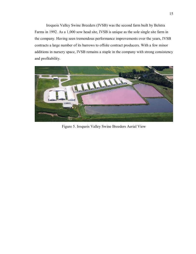
Iroquois Valley Swine Breeders (IVSB) was the second farm built by Belstra

Farms in 1992. As a 1,000 sow head site, IVSB is unique as the sole single site farm in

the company. Having seen tremendous performance improvements over the years, IVSB

contracts a large number of its barrows to offsite contract producers. With a few minor

additions in nursery space, IVSB remains a staple in the company with strong consistency

and profitability.

Figure 5. Iroquois Valley Swine Breeders Aerial View

16

In 1995, Pembroke Oaks Farms (POF) was built as our largest farm at the time

with 1,200 sows on one site. As another farm pushing the barriers of production, POF

also went through an expansion in 2006. Reaching its limits at the current site, a brand

new 2,500 sow unit was built at a new location. Extra finishing barns were also added to

the current location. After the expansion, POF continued its fierce performance requiring

the addition of another offsite finisher. JP Ag was added in 2011 to raise barrow pigs.

Figure 6. Pembroke Oaks Finisher Farm Aerial View

Figure 7. Pembroke Oaks Sow Farm Aerial View

17

Hopkins Ridge Farms (HRF) was built in 1998 as a 1,300 head unit and BGF’s

first multi-site farm. HRF saw tremendous performance and great health for many years.

During a time of transition and recognizing an opportunity for a new strategy, HRF was

converted into the BFG daughter nucleus site. HRF provides replacement gilts to IVSB,

MLF, POF and Legacy Farms.

Figure 8. Hopkins Ridge Sow Farm Aerial View

Figure 9. Hopkins Ridge Finisher Farm Aerial View

18

Built in 2002, Max-L Farms (MLF) was the fifth farm in the BGF family. As a

2,000 sow system, MLF is located in three different areas for sows, gilts and barrows.

Since 2002, MLF has seen record breaking production on a number of years. MLF also

uses a number of offsite contract finishers to assist in raising market hogs. MLF

continually pushes the boundaries for production.

Figure 10. Max-L Sow Farm Aerial View

Figure 11. Max-L Finisher Farm Aerial View

19

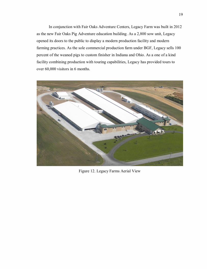
In conjunction with Fair Oaks Adventure Centers, Legacy Farm was built in 2012

as the new Fair Oaks Pig Adventure education building. As a 2,800 sow unit, Legacy

opened its doors to the public to display a modern production facility and modern

farming practices. As the sole commercial production farm under BGF, Legacy sells 100

percent of the weaned pigs to custom finisher in Indiana and Ohio. As a one of a kind

facility combining production with touring capabilities, Legacy has provided tours to

over 60,000 visitors in 6 months.

Figure 12. Legacy Farms Aerial View

20

2.4 Pig Production

In the past 20-25 years, the pig industry has seen vast amounts of changes from

technology improvements and increases in productivity. Genetic companies continually

push the bubble of efficiency in growth and production. Goals have become 35 pig per

sow per year with 2.0 feed conversions and 2.0 average daily gains (Strittmatter 2013).

Swine health has gone through tremendous strides as new biosecurity protocols are

implemented and new vaccines become readily available. All of this has created a viable

industry geared toward advancements. Farmers continually adapt and try to capture new

ways of improvement. Inherently, this also created the need for multiplication farms.

Reaching new performance levels meant finding and using females with the desired

genetic traits. Similarly, this lead to more sows being replaced in older herds. It was

quickly discovered that farms designed and run specifically for the purpose of selling

specialty gilts was much easier than keeping it in house. Farmers could see the

improvement in there herd while relieving some of the pressure for capturing the genetic

improvements. As a multiplier, BGF has been at the fore front of the genetic

improvement for a long time. As a vibrant business, BGF is looking into its core strategy

of gilt sales with the same goal as the whole industry; capturing improvements.

2.4.1 Genetic Multiplication

The genetic multiplication business is the link between genetic companies and

producers. Over the years, genetic companies like PIC or Geneiporc have developed

specific breeds of pigs that show traits desired by the pork industry. Today’s pig farmer

looks for four main characteristics: sow productivity, feed efficiency, growth rate and

carcass merit (Strittmatter 2013). These four things combined will allow for large

volumes of fast growing pigs that eat less and have a high value when sold to market.

These traits are passed down 50/50 from the male and female parents. Because boar

semen is easy to capture, can be diluted and used for a vast amount of producers, and has

quick turnover, it is more widely used to capture the genetic improvements in sow

performance and commercial growth. Unlike boar semen which is easily transported and

has high throughput, the limiting factor in genetic improvement is the need for live

females. As a large volume of the equation sows must also be replaced with younger

21

sows to keep performance levels consistent. These females are typically crossbred

females decedent from multiple parent genomes that exhibit the desired traits. It is the job

of the multiplication business to perform this intermediate cross breeding of specific

genetic breeds for producers to use as replacement sows.

Belstra Group Farms has two specific multiplication breeding patterns for PIC (1)

daughter nucleus gilt multiplication and (2) gilt multiplication. PIC uses three main

maternal lines as the basis for the daughter nucleus multiplication. The maternal lines are

synthetic purebred breeds of the landrace, large white and white duroc. As a daughter

nucleus, Hopkins Ridge Farms breeds the Line 3 maternal large white female to the Line

19 maternal white duroc male creating the PIC 1070. Iroquois Valley, Max-L and

Pembroke Oaks then breed the PIC 1070 back to the Line 2 maternal landrace male to

create the terminal Camborough 29 female. These C29 terminal females are gilts that are

sold to commercial farmer for replacement purposes. Breeding the C29 with terminal

boars (C359 or C327) create the terminal commercial market hogs. Ultimately, through

the long multiplication process starting from the maternal lines, the terminal commercial

pigs see all the desired characteristics of growth and efficiency desired by the producers

and packers (DeKryger and Hoek 2013). Appendix A illustrates the process.

2.4.2 Genetic Sales

As a core strategy, genetic multiplication must provide some incentive for BGF.

The incentives should cover: (1) higher production costs and lower efficiencies from

maternal production and (2) the demand for the genetic improvements being supplied to

the customer. During the production cycle, there are specific growth efficiencies and jobs

that create extra costs for BGF. Maternal and multiplication animals inherently have

poorer growth performance in feed conversions, average daily gains, lean percentages,

and mortalities. These four relative factors raise the cost for producing these pigs.

Simultaneously, labor costs also increase because additional chores are required

including additional procedures in sow units (i.e. taping underlines of baby gilts,

additional vaccination and treatment), as well as additional selection, tagging, and sorting

for gilt sales. To compensate for these additional costs, gilts are sold at premiums to

22

customers. This premium is used to cover any additional performance loss or production

costs seen on the farm.

Additional production cost is not the only reason for collecting the premiums. In

an industry where performance is key, capturing improvements on the farm in growth

efficiency and sow productivity allow for increasing sales and revenue. As a multiplier,

BGF is not only selling quality females, but it is selling the genetic improvements desired

by the customers. With an increasing demand for PIC genetics and the benefits it holds,

BGF sells the genetic potential at a premium. As an example, PIC improvements show a

0.13 increase in total born pigs per litter each year. If each sow was having 0.13 more

baby pigs per litter each year, that would equate to an additional $0.40 for every pig

weaned (DeKryger and Hoek 2013). This sort of potential can be seen over multiple

performance traits. Selling these genetic improvements and potential comes at a price,

thus another reason for BGF to use a premium on the gilt sales.

2.4.3 Production cycle

Pig farming follows a biological and systematic flow through the cycle to ensure

consistency and efficiency from production. Pigs are wonderfully gifted with timely and

predictable estrous cycles on top of very efficient growth rates, thus allowing producers

to utilize space and efficiencies throughout the facility.

For the purpose of this study, pigs can be classified three ways: (1) gilt or unbred

female pig (2) sow, female pig that has given birth (3) barrow, non-intact male pig.

Starting in the breeding barn, female pigs (sows) are typically bred first around 210 days

of age and 4-7 days after each sequential litter of piglets. A typical breeding cycle for

sows average 140-150 days with 2.4-2.5 litters per year. Female pigs are typically

artificially inseminated up to three times before implantation. Post-implantation of the

embryos, bred females are moved to a new location for the 115 day gestation period.

After gestation, the females are moved to the farrowing room for the birthing process.

Litters usually consist of 12-16 live piglets weighing 3-4 lbs. During the lactation period

in multiplier farms, piglets are processed, tattooed, given shots of iron, and gilts have

their underlines taped to protect their teats. Tape is removed 3-4 days later when tails are

23

removed. Sows will be moved back to the breeding barn after the baby piglets are weaned.

Baby piglets will stay with their mother for 21 days before being weaned off and moved

to the nursery.

After weaning, weaned pigs will be moved to three different possible locations

depending on the type and size of production unit: (1) nursery rooms at the main location,

(2) nursery rooms at offsite locations, (3) wean to finish buildings. These pigs will remain

in the nursery about 7 weeks until they grow to 60-65 pounds. After the 7 weeks, the pigs

are moved to finishing barns where they remain until they are sold. Pigs in wean to finish

barns remain there entirely. The finishing cycle takes about 15-16 week until the pigs

grow to 280-300 pounds. See Appendix B for a visual representation of the production

flow.

For identification purposes each litter is given an ID number referring to their

birth date. Once moved to the nursery, all the multiple litters in one nursery room are

given a new ID number referring to their wean date. When nursery pigs are moved to a

finishing barn, all the pigs in that one barn are given a separate ID group number. Each

finishing barn has roughly 3 different groups of pigs (closeouts) in a year.

The flow for multiplication farms varies slightly during the nursery and finishing

phases of production. Once a litter is weaned from the sow, the barrows (boys) and gilts

(girls) are separated in the nursery. Female pigs stay on the headquarter locations for

selection and sales, while male pigs are moved to off-site locations to be finished out.

Increased biosecurity measures are put in place at the main locations for breeding and

finishing. All employees must shower in and out to detract any diseases.

All supplies and equipment must be disinfected before entering the farm. Also, feed

trucks and maintenance vehicles must disinfect their tires when driving between farms.

To ensure the health of the pigs sold to the customers, these protocols must be

implemented.

During the 110 days in the finisher, gilts are selected and sold to customers for

replacement breeding pigs. Customer sales vary depending on the desired age, weight,

and number needed for replacement. Select gilts are sold at ages between 130 days to 170

days. Breeder Weaner gilts are sold younger than 130 days of age. Employees must select,

24

vaccinate, mark and ear tag each gilt for ID purposes. Gilt selection requires matching a

strict set of criteria. Figure 13 provides a picture of the selection characteristics.

Characteristics include appropriate size, healthy legs and feet, a balanced underline with

fourteen undamaged teats, healthy body condition (no abscesses) and proper body score

(not too fat, skinny, tall or short).

Figure 13. Gilt Selection Guidelines (Checkoff 2009)

25

CHAPTER 3. MODEL

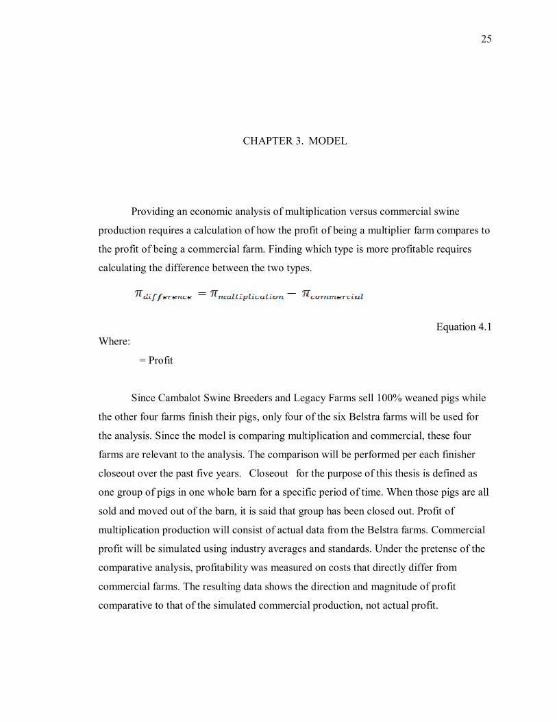
Providing an economic analysis of multiplication versus commercial swine

production requires a calculation of how the profit of being a multiplier farm compares to

the profit of being a commercial farm. Finding which type is more profitable requires

calculating the difference between the two types.

Equation 4.1

Where:

π = Profit

Since Cambalot Swine Breeders and Legacy Farms sell 100% weaned pigs while

the other four farms finish their pigs, only four of the six Belstra farms will be used for

the analysis. Since the model is comparing multiplication and commercial, these four

farms are relevant to the analysis. The comparison will be performed per each finisher

closeout over the past five years. “Closeout” for the purpose of this thesis is defined as

one group of pigs in one whole barn for a specific period of time. When those pigs are all

sold and moved out of the barn, it is said that group has been closed out. Profit of

multiplication production will consist of actual data from the Belstra farms. Commercial

profit will be simulated using industry averages and standards. Under the pretense of the

comparative analysis, profitability was measured on costs that directly differ from

commercial farms. The resulting data shows the direction and magnitude of profit

comparative to that of the simulated commercial production, not actual profit.

26

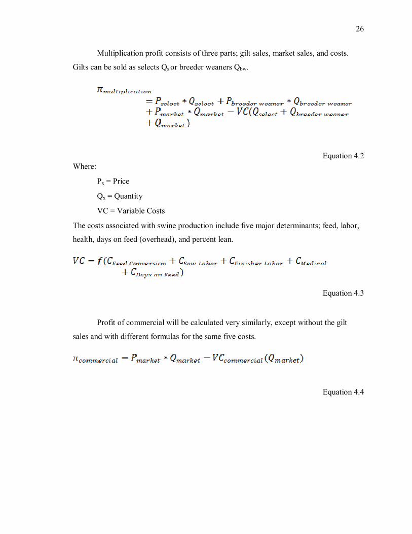
Multiplication profit consists of three parts; gilt sales, market sales, and costs.

Gilts can be sold as selects Qs or breeder weaners Qbw.

Equation 4.2 Where:

Px = Price

Qx = Quantity

VC = Variable Costs

The costs associated with swine production include five major determinants; feed, labor,

health, days on feed (overhead), and percent lean.

Equation 4.3

Profit of commercial will be calculated very similarly, except without the gilt

sales and with different formulas for the same five costs.

Equation 4.4

27

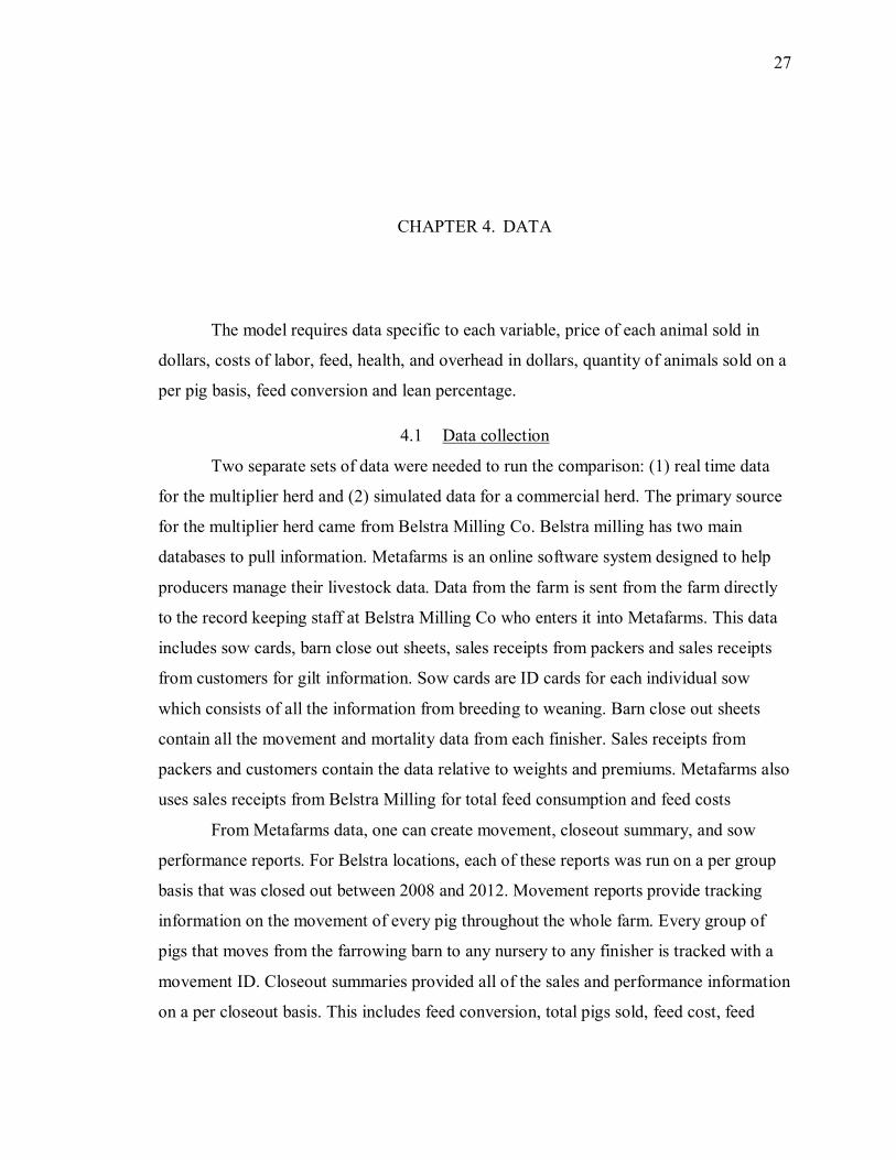
CHAPTER 4. DATA

The model requires data specific to each variable, price of each animal sold in

dollars, costs of labor, feed, health, and overhead in dollars, quantity of animals sold on a

per pig basis, feed conversion and lean percentage.

4.1 Data collection

Two separate sets of data were needed to run the comparison: (1) real time data

for the multiplier herd and (2) simulated data for a commercial herd. The primary source

for the multiplier herd came from Belstra Milling Co. Belstra milling has two main

databases to pull information. Metafarms is an online software system designed to help

producers manage their livestock data. Data from the farm is sent from the farm directly

to the record keeping staff at Belstra Milling Co who enters it into Metafarms. This data

includes sow cards, barn close out sheets, sales receipts from packers and sales receipts

from customers for gilt information. Sow cards are ID cards for each individual sow

which consists of all the information from breeding to weaning. Barn close out sheets

contain all the movement and mortality data from each finisher. Sales receipts from

packers and customers contain the data relative to weights and premiums. Metafarms also

uses sales receipts from Belstra Milling for total feed consumption and feed costs

From Metafarms data, one can create movement, closeout summary, and sow

performance reports. For Belstra locations, each of these reports was run on a per group

basis that was closed out between 2008 and 2012. Movement reports provide tracking

information on the movement of every pig throughout the whole farm. Every group of

pigs that moves from the farrowing barn to any nursery to any finisher is tracked with a

movement ID. Closeout summaries provided all of the sales and performance information

on a per closeout basis. This includes feed conversion, total pigs sold, feed cost, feed

28

consumed, total days on feed, percent lean, genetic sales, market sales, market weights,

group ID, start date and end date. Sow performance monitors provided the performance

data for sow farms on a weekly basis including pigs weaned, farrowing rates, and pre-

wean mortality.

In conjunction with Metafarms, Quickbooks is accounting software which

provides the balance sheets, health costs and labor costs for each farm. Labor costs were

pulled from Quickbooks on a per week basis and per group date range from 2008-2012.

This report included total employees, total hours and average wage. Multiplication

assistance and bookkeeping were also pulled from the same Quickbooks report.

Veterinary and medical costs reports were run from Quickbooks from 2008-2012. Each

yearly report had monthly charges broken out. The total cost for each month was then

added up and recorded.

The date of sale per closeout typically ranges over a one to two week period. Base

price for gilt and market sales was determined using the CME daily Eastern Corn Belt

carcass price. To capture the range of sale, weekly averages were calculated to represent

the price during the span of actual sales.

Data for commercial production was collected through multiple sources.

Performance differences between multiplier genetics and commercial genetics were

collected from the PIC sample herds and trials (Strittmatter 2013). This included feed

conversion, days on feed and lean premiums. Sow labor data required drafting a producer

questionnaire that would represent industry averages. Appendix C illustrates the

questionnaire sent out to representative producers in commercial production. Finishing

labor and overhead costs were calculated from formulas used by PIC contract finishing

division (Melody 2013).

4.2 Summary Statistic

In total, 1,092 individual groups (observations) were collected over from 2008-

2012. For every variable collected, the mean, median and standard deviation were

calculated. To summarize the results, each farm showed slight differences in their data.

Each farm showed slightly different results based on the size and strategy of each. Tables

1-4 illustrate the summary of all the data collected.

29

A correlation analysis was also done on the explanatory variables. Correlation

measures the linear association between any two variable in the equation. Having

correlation between the variables would tend to skew the results. There was little

correlation between the variables. See Appendix D for the correlation coefficients.

Table 1. Pembroke Oaks Farms 5 Year Summary Statistics Pembroke Oaks Farms Mean Median Standard Deviation

Price / Select $154.07 $157.67 $29.54 Quantity Select Sold 193.81 170.00 126.54 Average Select Weight 257.78 256.62 18.31 Price / Breeder Weaner $112.36 $110.96 $24.39 Breeder Weaner Sold 150.00 130.00 93.84 Breeder Weaner Weight 168.10 176.25 37.69 Percent Lean 0.54 0.54 0.01 Market Price $151.28 $158.14 $29.95 Quantity Market Sold 685.25 730.00 229.34 Total Revenue $139,924.53 $147,714.62 $58,060.08 Feed Conversion 2.90 2.89 0.17 Feed Cost $66,040.66 $69,500.54 $24,002.48 Sow Labor Cost $5,076.62 $5,128.97 $2,152.32 Finish Labor Cost $5,215.86 $5,814.33 $1,641.35 Health Cost $4,988.88 $4,643.05 $2,699.08 Days On Feed $7,906.91 $8,679.71 $2,729.50 Profit $50,695.60 $47,299.24 $33,172.17

30

Table 2. Max-L Farms 5 Year Summary Statistics Max-L Farms

Mean Median Standard Deviation Price / Select $156.02 $157.94 $29.18 Quantity Select Sold 303.60 297.5 140.93 Average Select Weight 265.19 261.013614 22.06 Price / Breeder Weaner $114.70 $114.13 $22.08 Breeder Weaner Sold 160.87 137.5 112.91 Breeder Weaner Weight 170.83 176.0879121 30.56 Percent Lean 0.54 0.5494 0.05 Market Price $147.32 $152.74 $30.03 Quantity Market Sold 621.25 711 253.40 Total Revenue $130,777.16 $129,825.44 $32,464.72 Feed Conversion 2.82 2.81606 0.14 Feed Cost $61,193.83 $58,745.16 $13,323.15 Sow Labor Cost $4,740.57 $4,494.33 $1,020.37 Finish Labor Cost $5,051.86 $4,510.00 $2,098.72 Health Cost $5,380.62 $5,175.12 $1,695.93 Days On Feed $8,002.98 $6,676.01 $2,839.30 Profit $46,407.31 $46,252.54 $26,478.80

31

Table 3. Hopkins Ridge Farms 5 Year Summary Statistics Hopkins Ridge Farms Mean Median Standard Deviation

Price / Select $154.18 $160.71 $31.64 Quantity Select Sold 138.39 126.00 79.37 Average Select Weight 248.92 250.97 35.13 Price / Breeder Weaner $113.67 $116.17 $21.32 Breeder Weaner Sold 131.89 101.00 89.58 Breeder Weaner Weight 158.86 160.83 27.10 Percent Lean 0.53 0.55 0.09 Market Price $144.37 $143.51 $32.14 Quantity Market Sold 711.14 732.00 212.86 Total Revenue $129,129.15 $132,723.08 $52,777.96 Feed Conversion 2.73 2.73 0.13 Feed Cost $58,368.32 $62,260.57 $19,281.85 Sow Labor Cost $6,561.40 $6,913.76 $2,654.65 Finish Labor Cost $4,475.70 $4,933.54 $1,421.48 Health Cost $6,163.39 $6,194.87 $2,789.71 Days On Feed $6,181.60 $6,926.72 $2,084.11 Profit $47,378.75 $45,201.72 $34,743.49

32

Table 4. Iroquois Valley Swine Breeders Farms 5 Year Summary Statistics Iroquois Valley Swine Breeders

Mean Median Standard Deviation Price / Select $142.94 $144.92 $25.87 Quantity Select Sold 108.14 100.00 57.98 Average Select Weight 246.39 248.64 14.69 Price / Breeder Weaner $111.45 $110.25 $20.50 Breeder Weaner Sold 149.86 136.50 81.51 Breeder Weaner Weight 170.16 169.29 14.96 Percent Lean 0.54 0.54 0.03 Market Price $145.62 $146.12 $31.31 Quantity Market Sold 386.82 357.00 169.31 Total Revenue $75,657.79 $69,812.95 $43,923.10 Feed Conversion 2.85 2.83 0.22 Feed Cost $36,454.45 $36,175.35 $18,827.79 Sow Labor Cost $3,038.90 $2,874.31 $1,711.41 Finish Labor Cost $3,016.73 $2,532.50 $1,805.66 Health Cost $3,477.12 $2,978.49 $2,249.77 Days On Feed $3,887.13 $3,181.97 $2,296.01 Profit $25,783.46 $17,256.31 $22,570.69

33

Distribution of the total data was also estimated through Stata to show the range

of the results for each variable. Figures 14-21 illustrate the distribution. Most variables

were relatively skewed as the data incorporated four farms of different characteristics and

sizes. Pembroke, for example, would sell higher number of gilts because it has 1,500

more sows. Offsite finishers vary from barns with 300 pigs up to 1,000 pigs which affects

the finishing costs and total days on feed. With lower performance as well, costs are not

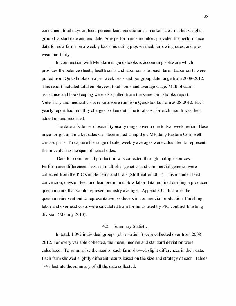
well distributed and inconsistent at these locations.

Figure 14. Distribution Summary for the Quantity of Select Gilts Sold.

34

Figure 15. Distribution Summary for the Quantity of Breeder Weaner Gilts Sold.

35

Figure 16. Distribution Summary for the Quantity of Market Pigs Sold.

36

Figure 17. Distribution Summary for the Average Feed Conversion per Group of Pigs.

37

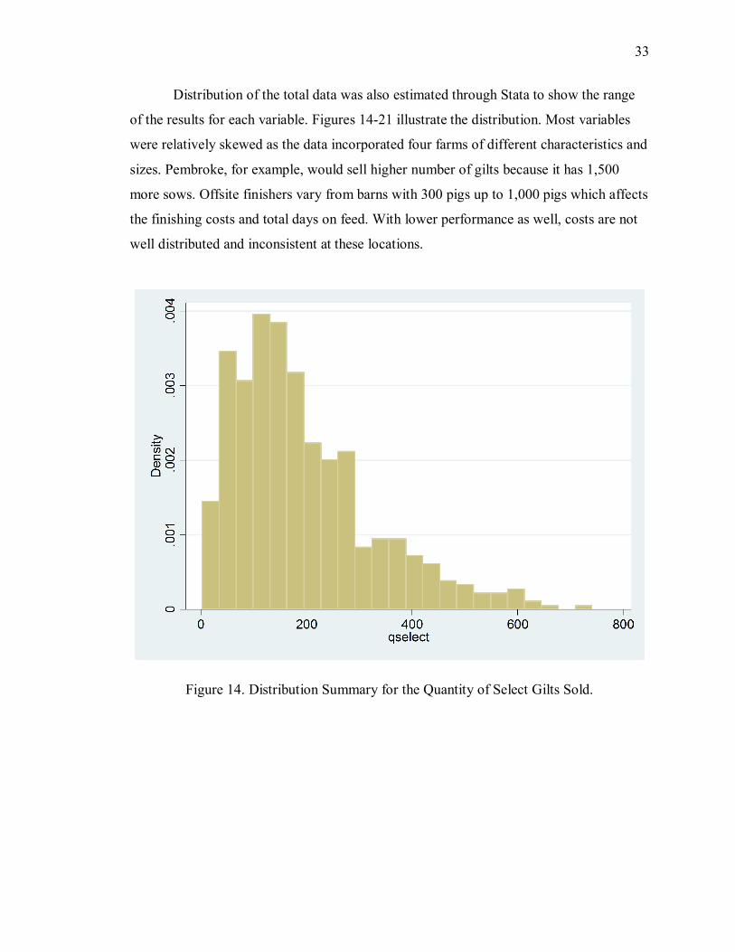
Figure 18. Distribution Summary for the Average Labor Costs on the Sow Farm per Week.

38

Figure 19. Distribution Summary for the Average Labor Costs on the Finishing Units for Gilts and Barrow Closeouts.

39

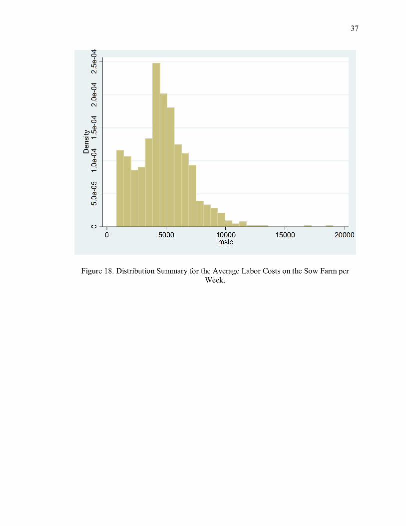
Figure 20. Distribution Summary for the Average Health Costs per Group of Pigs.

40

Figure 21. Distribution Summary for the Average Days of Feed Costs per Group of Pigs.

41

CHAPTER 5. METHODS

The purpose of this case study is to compare the profitability of multiplication swine

systems over commercial. In order to obtain enough observations and variation, data was

collected per each individual closeout over the past five years, “closeout” being defined

as one group of pigs in one whole barn during a specific period of time. First, each group

over the five years was collected and placed in an Excel spreadsheet. This included the

farm, specific site, group ID, gender, year of closeout, start date, close date, wean date,

wean week and total pigs sold. Data was pulled off of Metafarms closeout summaries.

Wean weeks were calculated as 45 days before finisher start date. In total, 1,092 separate

closeout groups over 22 sites were recorded.

5.1 Revenue

Revenue per group for each farm was collected using the total pig sales. Generally,

revenue for commercial farming is generated solely from market sales. In the case of

multiplication, revenue is determined from three sources: pigs sold for market, pigs sold

as select gilts and as breeder weaner gilts. Each source generated revenue through

different sale price and formulas. Gilts, both select and breeder weaner, receive specific

premiums as part of the price formula in order to cover the extra costs generated from

labor and performance.

Revenue per select gilt sold was calculated using the price per head multiplied by

the number of gilts sold per closeout. The number of gilts and total gilt weight was

collected off of the movement report from Metafarms. Using those numbers, the average

weight per gilt was calculated. Price per head was formulated using the weekly Eastern

Corn Belt base price per pound. The price was converted to live weight by multiplying

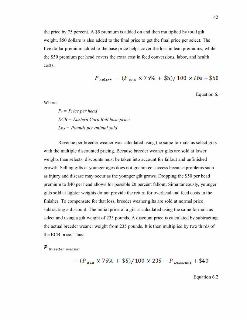
42

the price by 75 percent. A $5 premium is added on and then multiplied by total gilt

weight. $50 dollars is also added to the final price to get the final price per select. The

five dollar premium added to the base price helps cover the loss in lean premiums, while

the $50 premium per head covers the extra cost in feed conversions, labor, and health

costs.

Equation 6.

Where:

Px = Price per head

ECB = Eastern Corn Belt base price

Lbs = Pounds per animal sold

Revenue per breeder weaner was calculated using the same formula as select gilts

with the multiple discounted pricing. Because breeder weaner gilts are sold at lower

weights than selects, discounts must be taken into account for fallout and unfinished

growth. Selling gilts at younger ages does not guarantee success because problems such

as injury and disease may occur as the younger gilt grows. Dropping the $50 per head

premium to $40 per head allows for possible 20 percent fallout. Simultaneously, younger

gilts sold at lighter weights do not provide the return for overhead and feed costs in the

finisher. To compensate for that loss, breeder weaner gilts are sold at normal price

subtracting a discount. The initial price of a gilt is calculated using the same formula as

select and using a gilt weight of 235 pounds. A discount price is calculated by subtracting

the actual breeder weaner weight from 235 pounds. It is then multiplied by two thirds of

the ECB price. Thus:

Equation 6.2

43

Where:

Equation 6.3

Revenue for pigs sold to market was calculated from the price per head multiplied

by the total pigs sold as market hogs. This was calculated using the ECB base price plus

the lean premium received from the packer multiplied by the market carcass weight.

Market carcass weights for each group were pulled from packer receipts and Metafarms

movement reports. Lean premiums were derived using the formula set by the packers.

Equation 6.4

Where:

Equation 6.5 L = Lean premium

P = Price

M = Weight

Lean premiums for the commercial farms differ only by adding 1.1% to the % lean per

group. PIC charts the genetic difference between the two genetic types as 1.1%

(Strittmatter 2013).

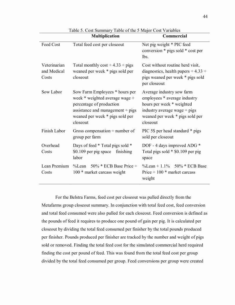
5.2 Costs

There are five major costs associated with production that have direct difference

between multiplication and commercial production. Table 5 illustrates how each cost was

derived.

44

Table 5. Cost Summary Table of the 5 Major Cost Variables Multiplication Commercial

Feed Cost Total feed cost per closeout Net pig weight * PIC feed conversion * pigs sold * cost per lbs.

Veterinarian and Medical Costs

Total monthly cost ÷ 4.33 ÷ pigs weaned per week * pigs sold per closeout

Cost without routine herd visit, diagnostics, health papers ÷ 4.33 ÷ pigs weaned per week * pigs sold per closeout

Sow Labor Sow Farm Employees * hours per week * weighted average wage + percentage of production assistance and management ÷ pigs weaned per week * pigs sold per closeout

Average industry sow farm employees * average industry hours per week * weighted industry average wage ÷ pigs weaned per week * pigs sold per closeout

Finish Labor Gross compensation ÷ number of group per farm

PIC 5$ per head standard * pigs sold per closeout

Overhead Costs

Days of feed * Total pigs sold * $0.109 per pig space – finishing labor

DOF - 4 days improved ADG * Total pigs sold * $0.109 per pig space

Lean Premium Costs

%Lean – 50% * ECB Base Price ÷ 100 * market carcass weight

%Lean + 1.1% – 50% * ECB Base Price ÷ 100 * market carcass weight

For the Belstra Farms, feed cost per closeout was pulled directly from the

Metafarms group closeout summary. In conjunction with total feed cost, feed conversion

and total feed consumed were also pulled for each closeout. Feed conversion is defined as

the pounds of feed it requires to produce one pound of gain per pig. It is calculated per

closeout by dividing the total feed consumed per finisher by the total pounds produced

per finisher. Pounds produced per finisher are tracked by the number and weight of pigs

sold or removed. Finding the total feed cost for the simulated commercial herd required

finding the cost per pound of feed. This was found from the total feed cost per group

divided by the total feed consumed per group. Feed conversions per group were created

45

from an extrapolated cumulative means low energy feed conversion from PIC (see

Appendix E). Using the actual net pig weight sold multiplied by the feed conversion,

number of pigs sold and cost per pound of feed, the total feed costs was able to be

determined.

Equation 6.6

Where:

C = Cost

M = Weight

FC = Feed Conversion

N = Total Head

Since Belstra Farms is supplying customers throughout the Midwest with

replacement gilts for their own herds, health is a top priority. Health costs are summed up

by a number of different line items and charges. These charges include but are not limited

to: herd visits, diagnostics, health papers, production supplies, veterinarian consulting,

vaccines, antibiotics, and equipment rental. Belstra Farms, in general, maintains an

extremely high standard regarding biosecurity and animal health. High health standards,

though, are not limited solely to multiplication farms. Because production performance is

correlated with high health standards, both multiplier and commercial producers have the

ability pay for the additional vaccine and antibiotic costs (Gillespie 2013). The difference

then between the two stems from multiplier farms having to continually prove a clean and

disease free status, while commercial producers tend to react to a possible dirty status

(Gillespie 2013). This additional cost equates to twelve herd visits per year instead of

four, monthly health papers, and routine monthly diagnostics. Belstra Farms receive

monthly bills from the vet for all charges. To distribute it appropriately among each

closeout, the monthly cost was divided by 4.33 for a weekly conversion, and then divided

by the number of pigs weaned that week since all relevant costs occur before the pigs are

weaned. That number multiplied by the pigs sold per each closeout resulted in the total

46

vet and medical costs for multiplication. The same formula for health cost was converted

to commercial production by removing 8 of the 12 herd visits, all the health papers, and

only the monthly routine diagnostics.

Equation 6.7

Where:

C = Cost

N = Total head

Calculating the total cost of labor requires allocating the cost of labor across pre-

weaning and post-weaning time frames. Not only is this a common practice in the

industry because of multiple off site finishing locations, but also because this model

captures the specific difference between multiplication and commercial. Before collecting

the necessary data, information for commercial production was needed for comparative

reasons. The producer questionnaire regarding labor was written and sent out to

representative producers of commercial production (see Appendix C for questions and

answers). Six anonymous producers responded to the questionnaire representing over

45,000 sows and nearly 1 million finishing pigs.

As a genetic multiplier, additional labor is needed to meet the industry and

customer standards. Multiplication has inherent responsibilities not seen on commercial

facilities. This can include: additional day one processing procedures, extra treatment

and litter management, selection, tagging and moving pigs. Not only is there additional

work with the animals, but general cleanliness and bio-security protocols take time and

effort as well. Because additional labor is required, BGF hires additional employees who

work longer hours with higher wages and compensation. There is a concerted effort for

BGF to retain employees as using the experience curve will help lower labor costs. With

higher employee tenure, BGF can lower its production costs from more experienced and

productive employees. For each BGF location, sow labor was divided up on a per weaned

pig basis. Starting in 2007, the number of pigs weaned each week was collected from the

47

sow performance report in Metafarms. Using reports from Quickbooks, the number of

employees working each week, total hours and average weight wage was calculated.

Because each farm consisted of two or more employees at a manager level and most

others at entry level, an average relative to the employee hierarchy was used to calculate

the average wage. Total wage per week was calculated by multiplying weekly employees,

average hours per week and average wage. Additional costs were added from BGF

management team that helps with bookkeeping, sales, and other various activities. The

total was divided by the number of pigs weaned per week to find the cost per head. Cost

per weaned pig was then multiplied by the number of pigs sold in the corresponding

group that closed out 45 days later.

Equation 6.8

Where:

C = Cost

E = Employees per week

W = Wage

PA = Production Assistance

The same formula was used for the simulated commercial producer using the

results from the questionnaire. Total number of employees per week was determined off

of the industry average 8 employees per 2,500 sow unit. This number changed depending

on the size of the farm but was held constant through every week. Similarly, the results

from the questionnaire provided the average hours worked per week and weighted

average age. Both numbers were held constant throughout the five years. The production

assistance in bookkeeping and gilt sales was not included in the calculation. Cost per

head varied according to the number of pigs weaned each week.

Historically, as farming operations grew in size and the number of pigs produced

at the sow farm, owners and operators did not have the capacity to finish all of the pigs

produced. This led to two types of units, specialized contract finishing units and crop

48

farmers diversifying into livestock. In both cases, contracts between the pig owner and

contractor were developed. These contracts described the responsibilities in costs for both

parties. Ultimately, the overall cost was expanded to a price per pig space. Included in the

price per pig space, along with a number of other variable and fixed costs, was the labor

cost. Labor cost for contract finishing in a wean-to-finish barn on average is

$10 per pig space or $5 per pig (Melody 2013). Wean-to-finish barns, in this context,

represent one barn that houses the pigs from 21 days of age until they are sold. Though

BGF does not use the wean-to-finish model for any of the farms, the concept and labor is

still comparable since each site still has nursery units. Thus finished labor per group was

calculated two ways. For those farms with BGF employees, total compensation during

the group’s closeout date was tallied and divided by the number of barns at the site.

Pembroke Oaks Farm, for example, which has seventeen finishing barns, divides the total

compensation for one group by seventeen. For offsite contract barns run by non-BGF

employees, the $5 per pig was multiplied by the number of pigs sold per closeout.

Similarly, the same $5 per pig formula was used for the simulated commercial farms.

Capturing the difference in overhead costs on a per group basis was done

similarly to the finish labor costs. As stated above, finishing contracts allocate the costs

on a per pigs space basis. Overhead costs include a number of variables including:

utilities, financing, contract labor, trucking, taxes, depreciation, insurance, repairs and

interest. Over the years, the standard for overhead costs on a per pig space basis has

averaged out to 10.9 cents. Whether or not pigs are in the barn, that same 10.9 cents is

being allocated to each pig space, thus putting high numbers of pigs through each barn

lowers the total overhead cost on a per pig basis. Using the total number of days the

group spent in the finisher (days on feed) from the Metafarms closeout summary

multiplied by the total pigs sold and the standard 10.9 cents per pig space gave the total

overhead cost per closeout. Because finishing labor was already calculated, the $5 per pig

multiplied by the total pigs sold was subtracted from the total cost. The difference

between commercial and multiplication overhead cost was determined by the average

days on feed generated from average daily gain. The genetic difference between the two

equates to multiplier herds averaging 4 extra days on feed (Strittmatter 2013). The

49

simulated numbers subtracted four days from the actual days on feed and multiplied it by

the total pigs sold and 10.9 cents per head.

5.3 Closeout Pairing

Each closeout recorded from each of the farms represented a single group. Each

group however was split into gilts and barrows once weaned from the sows. Groups on

the headquarter sites consisted of all the gilts and barrows (depending on the farm) while

all the offsite finishers were barrows. This showed other inconsistencies as home sites

were larger with newer barns and higher consistency while most of the offsite barns were

smaller and older. This raises the question as to whether the loss of profit and

performance from the offsite groups were also being compensated by the gilt sales. To

account for this, groups were combined to accurately measure the total profit of both

barrow and gilt sales. Since groups on headquarter sites and off-sites are given different

group IDs when moved to their respective locations, groups needed to be paired using the

date they were weaned from the sow farm. This was done by calculating the day and

week the pigs were weaned. Weaning dates and weeks were calculated by subtracting 45

days from the group’s start date. Groups that were weaned during the same week were

paired and added together to create one larger group. All of the variables were averaged

out or added together using pivot tables in Excel. These large groups created true

observations for profit with both barrow and gilts accounted for. Table 6 illustrates the

process. Once these closeouts were all added together, further analysis could be

completed to accurately measure the true profitability.

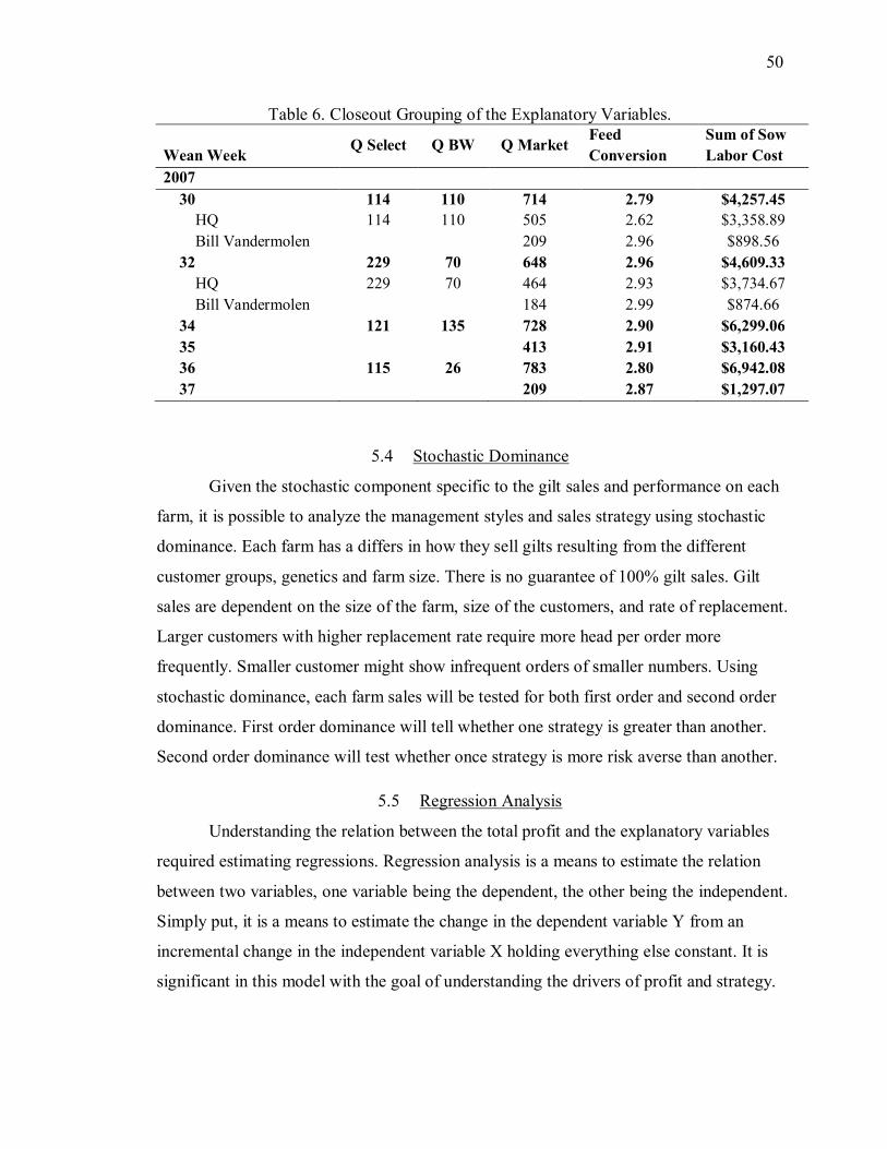
50

Table 6. Closeout Grouping of the Explanatory Variables.

Wean Week Q Select Q BW Q Market Feed Conversion

Sum of Sow Labor Cost

2007 30 114 110 714 2.79 $4,257.45

HQ 114 110 505 2.62 $3,358.89 Bill Vandermolen

209 2.96 $898.56

32 229 70 648 2.96 $4,609.33 HQ 229 70 464 2.93 $3,734.67 Bill Vandermolen

184 2.99 $874.66

34 121 135 728 2.90 $6,299.06 35

413 2.91 $3,160.43

36 115 26 783 2.80 $6,942.08 37

209 2.87 $1,297.07

5.4 Stochastic Dominance

Given the stochastic component specific to the gilt sales and performance on each

farm, it is possible to analyze the management styles and sales strategy using stochastic

dominance. Each farm has a differs in how they sell gilts resulting from the different

customer groups, genetics and farm size. There is no guarantee of 100% gilt sales. Gilt

sales are dependent on the size of the farm, size of the customers, and rate of replacement.

Larger customers with higher replacement rate require more head per order more

frequently. Smaller customer might show infrequent orders of smaller numbers. Using

stochastic dominance, each farm sales will be tested for both first order and second order

dominance. First order dominance will tell whether one strategy is greater than another.

Second order dominance will test whether once strategy is more risk averse than another.

5.5 Regression Analysis

Understanding the relation between the total profit and the explanatory variables

required estimating regressions. Regression analysis is a means to estimate the relation

between two variables, one variable being the dependent, the other being the independent.

Simply put, it is a means to estimate the change in the dependent variable Y from an

incremental change in the independent variable X holding everything else constant. It is

significant in this model with the goal of understanding the drivers of profit and strategy.

51

For this model, the independent variable is the difference in profit between multiplication

and commercial production. The dependent variables include; quantity of selects sold,

quantity of breeder weaners sold, quantity of market pigs sold, feed conversion, sow

labor costs, finishing labor cost, health cost, days on feed, and percent lean. To adjust for

seasonal variation during the five years, dummy variables were added for 2009 through

2012. The equation for estimating the regression is a follows:

Equation 6.9

Beta 0-13 represent the coefficients for each dependent variable. The resulting estimation

will provide the change in the response variable for every incremental change.

Estimating the first regression leaves some questions unanswered since some of

the variables are units of cost. Expanding the analysis out to further explain the drivers of

total profit required estimating regressions for labor. Using performance variables to

explain sow and finishing labor will provide a better understanding of what is driving

labor cost and ultimately the difference in profit. This was done using the following

equations:

Equation 6.10

Equation 6.11

52

Sow labor costs is a product of numerous variables, although due to high

correlative properties, it can be summed up in three key drivers; farrowing rate, pre-wean

mortality and total pigs weaned. Each variable was recorded on a per week basis.

Farrowing rate pertains to the percentage of sows that are bred and have babies. For

example, 90% farrowing rate equates to 90 out of 100 sows bred giving birth. Reasoning

states that farrowing rates drive the change in cost because a higher or lower percentage

of sows having babies affect the amount of labor. Pre-wean mortality is the percentage of

baby pigs that die before they are weaned from the sow, the higher the percentage, the

higher the mortality rates. The total number of pigs during the 21 day time period has an

effect on the total labor cost during that time. Total pigs weaned is the number of pigs

weaned from the sow. If more pigs are weaned for example, then the cost of labor

changes as well.

Finishing labor cost is pretty standardized within the industry. PIC uses the

average of five dollars per head for commercial market pigs (Melody 2013). The driver

of finishing labor cost for multiplication can be narrowed down to the number of select

gilts and breeder weaners sold per group. Gilts require additional work in the finisher.

This leads to more attention and longer time spent in each finisher than normal. If more

gilts are sold out of a group, the extra cost should be reflected in the regression. Thus, the

gilt and market sales per group are good used to estimate finishing labor cost.

The regressions above are estimated on the incremental changes consistent with

the specific variable. The quantity of gilts or market sold is a change in one pig. The

change in days on feed is by one day. Though this is significant when looking at short

term analysis of drivers in profitability, it only gives part of the analysis for what is

driving profitability. To analyze true impact of the variables, the elasticity for a percent

change in each variable was estimated to determine the impact of incremental changes on

the difference in profit. Using the same equation and results from the regression, the

elasticity was found inserting the mean for each variable, and by increasing one variable

at a time by one percent. The percent change in profit for each variable resulted in the

elasticity. This one estimated nine different times, increasing one variable one percent

while holding the other eight constant.

53

CHAPTER 6. RESULTS

Following the original hypothesis, three questions needed to be answered; were

the farms more profitable compared to the simulated commercial herd, is there stochastic

dominance between the four farms, and how are the explanatory variables related to the

overall profit of multiplication?

6.1 Profitability

Answering the first question is to determine whether or not the core strategy of

gilt sales is worth the investment. As mentioned in The Breakthrough Imperative,

understanding true profitability is important for a business strategy. The results looked

beyond whether the farms were profitable and into whether the farms were more

profitable than typical farms. True profitability in this case becomes whether the extra

money, labor and time is being compensated enough. Greater profitability in

multiplication was determined by whether the total profit of multiplication was greater

than the simulated profit of a commercial herd. Barrow and gilt groups were added

together by wean week to create larger groups that encompass both gilt and barrow sales.

The total difference in profit from the combined group was summed up per year to

measure profitability. The results varied by each farm. Table 7-10 shows the yearly

summaries.

54

Table 7.Summary of the Difference in Profitability for Pembroke Oaks Farms. Sum of π Multiplication Sum of π Commercial Difference

2007 $ 1,335,633.36 $ 1,082,522.11 $ 253,111.23 2008 $ 2,643,273.61 $ 2,459,654.32 $ 183,619.27 2009 $ 2,443,432.25 $ 2,382,973.07 $ 60,459.14 2010 $ 4,498,608.33 $ 4,293,058.58 $ 205,549.86 2011 $ 4,765,718.75 $ 4,816,657.80 $ (50,939.00) 2012 $ 1,706,067.22 $ 1,854,067.62 $ (148,000.39) Grand Total $ 17,392,733.52 $ 16,888,933.50 $ 503,800.11

Pembroke Oaks Farms (POF) had years of both more and less profitability than

what it would have been as a commercial site. The highest years of profitability were in

2007 and 2010. A big contributor to the lower total profit in 2008 and 2009 was a period

of low hog prices. Prices during that time reached significant lows creating a difficult

period for profitability. 2010 saw an increase in prices and gilt sales allowing for a highly

profitable year. A few variables occurred in 2011 and 2012 creating some lower profits

for multiplication farms. As productivity grew at POF, new spaces needed to be created.

JP Ag was bought and remodeled as a barrow finisher. Performance at that location was

sub-standard as it was an older barn with some new management.

Around the same time in 2011 and 12, the premium gap between commercial

sales and gilt sales was growing closer. As lean premiums and market sizes continued to

grow, the premium for gilts remained the same. Essentially, commercial sales were

seeing a rise in the total revenue, while multiplication sale followed a slower increase

from flat based gilt premiums. This led to premiums not covering the total costs like

before.

55

Table 8. Summary of the Difference in Profitability for Iroquois Valley Swine Breeders. Sum of π Multiplication Sum of π Commercial Difference

2007 $ 362,166.78 $ 334,245.51 $ 27,921.27 2008 $ 1,017,155.83 $ 934,817.44 $ 82,338.40 2009 $ 936,850.88 $ 912,269.09 $ 24,581.78 2010 $ 1,837,116.41 $ 1,921,165.31 $ (84,048.82) 2011 $ 2,211,584.15 $ 2,274,228.02 $ (62,643.92) 2012 $ 906,060.91 $ 941,634.42 $ (35,573.53) Grand Total $ 7,270,934.96 $ 7,318,359.79 $ (47,424.82)

Iroquois Valley Swine Breeders (IVSB) resulted in fewer profits than a

commercial farm would have seen. Though having some stronger years in 2008 through

2009, it dropped off in the later years. This can be attributed to the same price gap

mentioned before, but IVSB saw a few other variables as well. In 2010 and 11, IVSB

contracted mycoplasma hyopneumoniae, a respiratory disease in pigs. Though it has

relatively little effects across performance when kept under control, it can cause a few

problems when it flairs up. It can also dissuade customers from buying gilts if the gilts

are already myco-negative and do not want to deal with the disease. Along with the

disease problem, IVSB has multiple offsite finishers that it uses for barrow pigs. These

offsite finishers though, do not have stellar performance. This ultimately drags the total

profitability lower and creates more burden on selling more gilts. Followed up by a few

years of low gilt sales brings the total profit lower than a commercial herd.

56

Table 9. Summary of the Difference in Multiplication for Hopkins Ridge Farms. Sum of π Multiplication Sum of π Commercial Difference

2007 $ 402,805.78 $ 447,591.98 $ (44,786.20) 2008 $ 1,310,013.94 $ 1,337,864.63 $ (27,850.69) 2009 $ 1,297,027.05 $ 1,350,415.49 $ (53,388.44) 2010 $ 2,093,569.58 $ 2,070,732.93 $ 22,836.65 2011 $ 2,400,791.17 $ 2,365,926.27 $ 34,864.90 2012 $ 1,118,724.69 $ 1,051,500.49 $ 67,224.20 Grand Total $ 8,622,932.21 $ 8,624,031.79 $ (1,099.58)

Hopkins Ridge Farms (HRF) also saw less profitability then the simulated

commercial herd. Unlike IVSB though, this was due to less profit in the earlier years.

During 2008 and 2009, HRF gilt sales were really low. HRF was coming off a period of

transition to producing purebred gilts as a daughter nucleus site for the Belstra Group

Farms. From that period of low gilt sales came the lower profitability. In 2011 and 2012,

HRF made a decision to start producing and selling both purebred and crossbred 1070

gilts. This decision stemmed from the low gilt sales seen in previous years. Since that

change, Hopkins has seen much high sales resulting in more profitability in later years.

Further extension of the research into 2013 quite possibly would have shown even higher

profitability resulting in net positive profitability over commercial herds.

57

Table 10. Summary of the Difference in Multiplication for Max-L Farms. Sum of π Multiplication Sum of π Commercial Difference

2007 $ 817,980.42 $ 746,451.12 $ 71,529.28 2008 $ 2,303,809.94 $ 2,014,758.31 $ 289,051.61 2009 $ 2,039,237.43 $ 1,868,979.75 $ 170,257.71 2010 $ 3,365,255.85 $ 3,266,530.45 $ 98,725.36 2011 $ 3,503,223.33 $ 3,496,326.59 $ 6,896.77 2012 $ 1,736,795.96 $ 1,579,194.65 $ 157,601.31 Grand Total $ 13,766,302.93 $ 12,972,240.87 $ 794,062.04

Out of the four farms, Max-L Farms (MLF) saw the greatest profits over the five

years. The results were not as expected. From discussions with BGF, Max-L had a period

of time with low gilt sales and lower performance. This was expected to show up in the

results during 2008-2009. Lower performance and sales must have shown up in 2010-

2011 which shows a much lower difference in profitability. The high profits in 2008-

2009 can possibly be attributed to unrecognized high performance in productivity and

feed conversions while keeping labor costs lower. Max-L was the first farm to ever hit 30

pigs per sow per year in 2007. Having that high of performance for five straight years

helps improve profitability.

These results proved consistent with the original hypothesis. The additional

revenues from gilt sales compensates for the additional costs and performance loss. There

were years where farms earned higher revenues compared to commercial farms, however

there were also years where farms saw fewer profits than commercial farms (figure 22).

This was to be expected as sales and performance, through the years, has varied from

farm to farm. No two farms are the same in customers, size or performance. Each farm

has different influences over the last five years creating variance in profitability. Between

the four farms though, there was definite profitability over commercial farms (figure 23).

It is interesting to note from figure 23, that the trend of profitability for the four farms in

inverted when compared to the market price during those four years. This is in large part

because the premium for gilts is a flat rate per head. Thus, when market prices are low,

the margin between gilt sales and commercial is much wider, but as the market prices

increase the margin decreases making commercial profits closer to gilt multiplication.

58

Figure 22. Difference in profit per farm over five years.

59

Figure 23. Total difference in profit over five years

6.2 Stochastic Dominance

The gilt sales strategy was evaluated for the four farms, Max-L, Iroquois Valley

Swine Breeders, Pembroke Oaks Farm and Hopkins Ridge Farms. The four variations are

illustrated in Figure 20. The cumulative density functions show that no first order

dominance was found between any of the farms. It also shows that no second order

dominance was found either. All negative observations are relatively similar due to the

sales of barrow pigs. There is no difference in the variation of barrow pig sales between

farms. On the positive side, there is a much more noticeable variation in the profitability

between farms. Max-L Farms outperformed the other farms in profitability on the

positive side. This can be directly correlated to the higher percentage of gilts being sold.

Gilts sales incorporate the premiums which in turn compensate the low performance and

costs. As gilt sales increase, so does the opportunity for profit, but increased gilt sales

also means higher risk in that if the gilts are not sold then there are no premiums. Thus

there is more reward incorporated with selling more gilts. Typically, gilts sales between

the four farms ranges from 20-40% of total sales. Max-L, in this case, has larger average

60

gilt customers with higher replacement rates. This draws a higher percentage of gilts out

of Max-L’s total sales. As seen in summary statistics, Max-L sells roughly 110 more

select gilts then the Pembroke Oaks Farms, 165 more select gilts then Hopkins Ridge and

195 more gilts then Iroquois Valley. The standard deviation for the select sales from

Max-L is high at 140.93 gilts sold, but having a higher risk sales strategy will bring a

higher variation in the amount sold. Max-L’s strategy in larger customers proves to have

higher risk because if larger customers stop purchasing gilts, it will create a larger hole in

the gilt sales compared to smaller customers.

Figure 24. Cumulative Density Function for the Profitability of the Max-L, Pembroke

Oaks, Iroquois Valley, and Hopkins Ridge.

61

6.3 Regression Analysis

Regression analysis determines the key drivers on profitability for each farm. As

defined in this study, it measures a change in the difference in profitability from

incremental changes in one variable holding all other constant. The size and direction of

the coefficients on the variables defines the significance of the explanatory variable. The

nine variables include select sales, breeder weaner sales, market sales, feed conversion,

sow labor, finishing labor, health costs, days on feed and percent lean. Table 11 illustrates

the estimated regression on the explanatory variables for difference in profit. Included in

the table are the coefficients and standard errors for each variable.

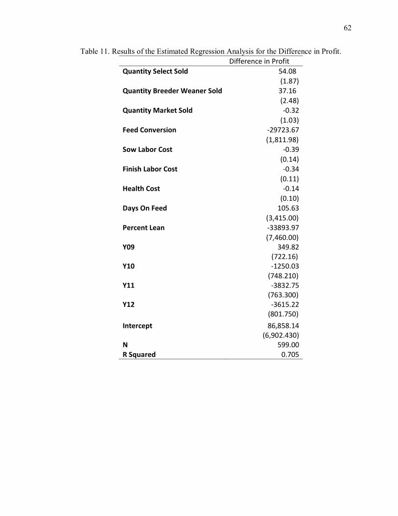
62

Table 11. Results of the Estimated Regression Analysis for the Difference in Profit. Difference in Profit

Quantity Select Sold 54.08 (1.87)

Quantity Breeder Weaner Sold 37.16 (2.48)

Quantity Market Sold -0.32 (1.03)

Feed Conversion -29723.67 (1,811.98)

Sow Labor Cost -0.39 (0.14)

Finish Labor Cost -0.34 (0.11)

Health Cost -0.14 (0.10)

Days On Feed 105.63 (3,415.00)

Percent Lean -33893.97 (7,460.00)

Y09 349.82 (722.16)

Y10 -1250.03 (748.210)

Y11 -3832.75 (763.300)

Y12 -3615.22 (801.750)

Intercept 86,858.14 (6,902.430)

N 599.00 R Squared 0.705

63

A significant driver in this analysis was feed conversion. Every one unit of an

increase in feed conversion (i.e. 2.5 to 3.5), would equate to a drop in the difference in

profit of $33,062.5/group. More precisely, every tenth of an increase in feed conversion

(2.5 to 2.6) equals a drop in the difference in profit of $3,306.25/group. With such small

differences leading to larger changes in profit, this becomes an important variable to

manage properly. In the case of finishers that might vary in size and age, feed conversion

can have a large effect on total revenue.

Lean percentage was another variable that had a potentially significant impact on

the difference in profitability. Every one percent increase in lean percentage (55% to

56%) lead to a drop in the difference in profit of $2,928.86/group. The variation in lean

percentage between the four farms is relatively small with an average standard deviation

of 5%. Using a realistic measurement in tenths of a percent equate to differences in profit

of $292.86/group.

As expected, both select and breeder weaner sales increase the difference in profit

for every one pig sold by 53.36 and 34.83 respectively. This estimation fits very accurate

with the analysis since the premium per head on select gilts is 50$ and 40$ per head for

breeder weaners. So if one additional gilt was sold, the difference in profit would be that

premium of $50 or $40 dollars. Market sales were not statistically significant in the

regression. Thus the quantity of market pigs sold does not accurately measure the change

in the difference in profit. This is not unexpected as the market price did not correlate

with a positive difference in profit. This is attributed to barrow sales having lower

performance.

Using the actual days on feed performance data showed an increase in profit of

$83.35/group for every one extra day on feed. This was different than expected since

more days on feed would assume higher costs to the producer and a lower difference in

profit. Simple reasoning though can explain the inverted direction from pigs growing

larger the longer they are in the barns. Larger pigs have higher revenues due to the price

of pork being on a per pound basis.

Sow labor cost, finishing labor cost, and health costs all resulted in small

coefficients. Each variable showed the total difference in profit decreasing with an

64

increasing costs, but because these three variables were regressed on a per dollar basis, a

change in one dollar in costs has a small impact on the total difference in profit. Using a

performance based parameter with a different unit of measurement provides more

accurate results for the key drivers of profitability. To incorporate the performance

measures driving labor costs, further regressions on labor were estimated to explain those

drivers. Three main explanatory variables were choses for sow labor and finishing labor.

Sow labor is measured easiest by the production of piglets, so farrowing rate, pre-wean

mortality, and pigs weaned were the three variables. Similarly, finishing labor is largely

driven by the number of pigs and type of pigs moving through the farms, thus selects sold,

breeder weaners sold and market pigs sold were the three variables. Table 12-13

summarizes the results from the regression.

Table 12. Results for the Estimated Regression Analysis on the Sow Labor Costs. Sow Labor Costs

Farrowing Rate -3807.04 (652.29)

Pre-wean Mortality 1151.66 (1,327.00)

Total Weaned Pigs 3.23 (0.08)

Intercept 5,760.69 (638.69)

N 1,152 R Squared 0.608 Prob > F 0.0000

Sow labor cost, done on a per week basis, show consistent results with what was

expected. Farrowing rate shows a decrease in the cost of $3,807.04/week for every 0.1

increase in farrowing rate. This can also be equated to a $380.74/week decrease in cost

for every 1% increase in farrowing rate (89%-90%). This result proves quite applicable

since lower farrowing rates cause employees to work harder. If farrowing rates drop,

employees put in more effort to raise it. If farrowing rates are high, employees are less

inclined to put efforts towards the breeding and farrowing.

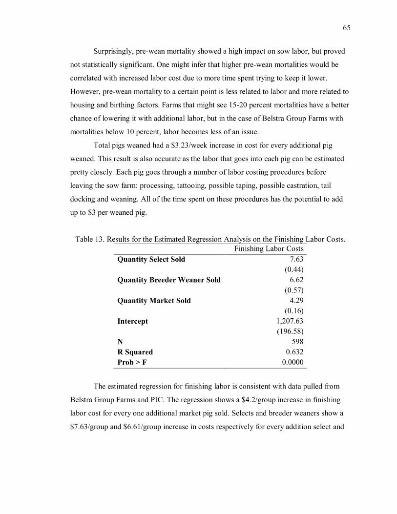
65

Surprisingly, pre-wean mortality showed a high impact on sow labor, but proved

not statistically significant. One might infer that higher pre-wean mortalities would be

correlated with increased labor cost due to more time spent trying to keep it lower.

However, pre-wean mortality to a certain point is less related to labor and more related to

housing and birthing factors. Farms that might see 15-20 percent mortalities have a better

chance of lowering it with additional labor, but in the case of Belstra Group Farms with

mortalities below 10 percent, labor becomes less of an issue.

Total pigs weaned had a $3.23/week increase in cost for every additional pig

weaned. This result is also accurate as the labor that goes into each pig can be estimated

pretty closely. Each pig goes through a number of labor costing procedures before

leaving the sow farm: processing, tattooing, possible taping, possible castration, tail

docking and weaning. All of the time spent on these procedures has the potential to add

up to $3 per weaned pig.

Table 13. Results for the Estimated Regression Analysis on the Finishing Labor Costs. Finishing Labor Costs

Quantity Select Sold 7.63 (0.44)

Quantity Breeder Weaner Sold 6.62 (0.57)

Quantity Market Sold 4.29 (0.16)

Intercept 1,207.63 (196.58)

N 598 R Squared 0.632 Prob > F 0.0000

The estimated regression for finishing labor is consistent with data pulled from

Belstra Group Farms and PIC. The regression shows a $4.2/group increase in finishing

labor cost for every one additional market pig sold. Selects and breeder weaners show a

$7.63/group and $6.61/group increase in costs respectively for every addition select and

66

breeder weaner sold. Since gilts require the additional selection, tagging, and vaccination,

the additional 2-3 dollars more in costs are appropriate for gilt sales

Table 14. Elasticity comparison between the key variables

Elasticity

Quantity Select Sold 0.021

Quantity Breeder Weaners Sold 0.012

Quantity Market Sold -0.001

Feed Conversion -0.210

Sow Labor Cost -0.006

Finish Labor Cost -0.005

Health Cost -0.002

Days on Feed 0.030

Percent Lean -0.046

From the estimated elasticity results on the variables, feed conversion proved to

be the largest driver of the change on the difference in profitability. A one percent

increase in feed conversion has the largest percentage change in the difference in profit.

Compared to the quantity of gilts sold, increasing feed conversion will largely decrease

the difference in profit between multiplication and commercial producers. This is

consistent with the first regression. Though it was at first thought to be a minor variable

due to overhead being relatively fixed over a large number of animals, days on feed

actually had one of the higher elasticity results. A possible reason for the high elasticity

on the difference in profit is the overall weight gain during the few extra days. If prices

are high, the few more pounds balances out the overhead costs by higher revenues.

Though percent lean also had a larger elasticity, the variation in percent lean for maternal

line pigs is very small making it difficult to increase. Overall, the estimated elasticity

results did not differ much in the relative impact seen in the original regression analysis.

Feed conversion is still the top priority for solid management.

67

CHAPTER 7. CONCLUSIONS

The agriculture industry is experiencing unprecedented variation in market prices

with additional influences through disease economic factors. Land values have reached

all-time highs throughout the Midwest, while corn prices start to return to normal falling

from record highs. Diseases including Porcine Epidemic Diarrhea Virus (PEDv) are

creating added pressure and distress throughout the pork industry as more and more herds

contract the virus. The University of Missouri estimates 1,373 confirmed cases in 19

states with those numbers continually increasing (Plain and Brown 2013). As an

intestinal disease that slows growth and causes high pre-wean mortality in younger pigs,

PEDv causes large ripple effects in the availability and sale of pork across the US. As an

external factor affecting the business of multiplication and pig production, it is imperative

that business strategies among farmers and agribusiness be strong and resilient in order to

overcome such variation and uncertainty in the industry.

7.1 Profitability

The answer to the main question “are your products truly profitable” is yes. The

results from the four Belstra Group Farms showed multiplication pig production can be

more profitable than commercial production when done correctly. As a core strategy for

BGF, the extra cost in health and labor coupled with the loss of performance in feed

conversion and average daily gain (days on feed) is being compensated by the premiums

received for gilt sales. The $5 added to the price is making up for the lean premium loss

while the $50 and $40 for the select and breeder weaners respectively, is providing the

additional costs for performance loss. This is shown by MLF and POF both being more

profitable than the commercial counterpart.

68

This, however, does not hold true always. There is still high risk in multiplication

farms being less profitable than a commercial counterpart. IVSB and HRF both show

examples of this. This can be a result of many factors affecting the farms, the primary

reason being low gilt sales. Higher percentages of gilts need to be sold to collect the

desired premiums. In the case of both IVSB and HRF, periods of low gilt sales resulted in

lower comparative profits. Once more gilts started to be sold, higher profits were seen.

Diseases can also play another large role. In the case of IVSB, having mycoplasma

created increased costs and lower performance. Adding that on top of the current

additional costs creates a situation where the premiums can’t cover it. This health risk

creates the high importance to remain disease free at every farm. Thirdly, management at

offsite locations must be held in high standards. If finishers that house barrow pigs are

showing subpar performance, it creates a drag which makes it harder for gilt premiums to

compensate for. In the case of IVSB, a couple offsite finishers tended to show feed

conversion well above 3.0 as well as high mortalities. Subsequently, this created really

high feed costs and lower revenues. Keeping a better watch on not only the care and

management of the pigs but also the building and housing structure can allow for better

performance and lower drag at barrow finishers.

7.2 Factors Affecting Multiplication Strategies

From a pure profitability standpoint, gilt multiplication proved more profitable

when the conditions were met. Though the economic implications point to more profits

stemming from the multiplication strategy, certain non-quantifiable variables must be

taken into account. Most importantly, the strategic implementation of health and

biosecurity must be taken into account. As mentioned before, multiplier herds must meet

extreme health standards and consistently prove a clean status. Accomplishing this starts

with the location. Multiplier herds require 3-5 miles from any other pigs in low density

regions. Areas with large pig populations tend to deter multiplier farms because of the

possible disease transmission. Along with the location is the strategic implementation of

biosecurity. This not only takes into account the health costs, but includes the strategic

planning, adapting and controlling of biosecurity measures. Buildings are designed and

protocols are implemented to increase the biosecurity measures.

69

The effort of selling gilts is another variable that can be hard to quantify. There is a

similar managerial effort of selling market hogs in multiplier herds as there is in a

commercial herd. Gilt sales, though, incorporate additional interaction and

communication with a customer base. Some of this dollar amount was captured in the

production assistance in the sow labor mentioned earlier, but the constant contact with

other producers must be included as well. Interacting with the customers and trying to

find agreeable terms in a contract can be tedious and tasking.

Overall, there is a substantial amount of additional risk when having a

multiplication strategy. Because of the additional variables in multiplication, the strategy

requires gilts sales to be high in order to be more profitable. Gilts sales are never

guaranteed and can be affected by multiple factors. Whether it is disease, bad relations

with customers or simply poor management, if the gilts are not sold then the whole

strategy becomes less profitable and the products are not truly profitable as define in

“The Breakthrough Imperative.”

7.3 Going Forward

There are a number of things that the BGF can take away from this study as they

continue to move forward. Being the first in depth look into a business decision dating

back 20 years, the management team can be assured that their core strategy is profitable

and worthwhile. Knowing that it is a correct strategy allows them to look past the

question of “why” and focus on how to make it better. There are a few insightful

takeaways from this study.

First and foremost, gilt sales must be top priority. Though this might seem

obvious from the business standpoint, the emphasis needs to be clear. Selling low

lpercentages of gilts does not account for the additional costs. The goal should be to sell

as many as possible. This was displayed in the results for farms like HRF and IVSB when

they had years of lower profitability compared to the commercial herd. Whether it was

lack of effort from the management team, lack of buying customers or other various

reasons, the absence of gilt sales affects true comparable profitability. Some possible

actions for BGF might include: (1) hiring sales specific individuals who have the

responsibility to sell gilts. Having someone actively interacting with customers and

70

looking for opportunities can help increase the percentage of sales. (2) Increase their size

of operation. Like most industries, bigger operations or companies continually look to

grow in order to capture more opportunity and profits. In the case of BGF, expansion of

specific farms or the addition of new multipliers will not only just add more pigs, but also

mean more available gilts to sell. As seen by the two larger farms, POF and MLF, there is

not only a greater difference in profit between multiplier and commercial, but a larger

profit pool in general. (3) Put greater attention and focus on gilts health and selection

rates. BGF currently uses a 70% selection rate at each farms, meaning only 70% of the

gilts placed in the farm are available for non-market sales. This is generally the case

because gilts do not always meet the specific criteria needed. If the gilts have a bad set of

teats, inappropriate number of teats, health problems, or poor body conditions, they do

not meet the criteria and are not selected for sale. As a customer driven product, BGF

needs to sell high quality animals. If additional effort was placed ensuring better quality

of gilts, more gilts would be available for customer sales.

Secondly, growth performance and efficiency drives a large part of the associated

costs. This can be seen from the estimated regression on the difference in profit and on

sow labor costs. Primarily, feed conversion has the largest impact. Though it can be

attributed to genetic differences on multiplication farms, there is still a management

factor when raising finishing pigs. Poor management can cause the feed conversion to

rise if feed rations and diets are not kept in check. Another element affecting feed

conversion is the housing conditions. Older barns with poor ventilation, crowded pens

and dirty conditions can increase feed conversion. Thus, BGF can put an emphasis on

improving the management and housing conditions for raising both gilt and barrow pigs.

Addition effort can prove very beneficial if growth performance is increased. Farrowing

rate is another example of how performance and efficiency can drive cost up or down.

From the regression alone, the results show thousands of dollars extra per week in costs if

farrowing rates are low. Continually reaching higher farrowing rates saves BGF money.

Thirdly, they must continually strive to reduce the risk of any health problems.

Multiplication farms must constantly prove they are clean and disease free. This is to

assure the genetic company and the customers that the replacement gilts are healthy and

71

in good condition. If BGF contracted some sort of disease, their gilt sales drop to zero as

customers try to avoid their herds from getting sick. Spending a significant amount of

time strategizing and implementing procedures reduce this risk. A couple possibilities

that BGF already use or could use include: reducing the traffic around the farm,

disinfecting vehicle tires, little movement between farms and increased preventative

treatment. Though disease in general has a large impact on production for any farm, it has

more of a negative impact for multiplication purposes.

7.4 Additional Research and Future Work

Due to the design of the model, one of the limitations was collecting real time

commercial data. The study consisted of very accurate and consistent data based off of

industry research and standards. For a more complete analysis, comparing actual

multiplication data against actual commercial data could provide further results and

conclusions. Another option would be adding variation in the simulated commercial herd.

The simulated commercial herd had data sets that remained constant throughout the five

years. Adding some variation in the data could create more depth in the analysis and

comparison. Some of the variation could be added to lean percentages, market weights,

feed conversions and sow labor.

Another possibility would be to add in additional variables. This study incorporated

the five main variables that were most relevant in cost and performance. Some of these

variables have the potential to be broken down further, or other new variables could also

be added. This might include variables such as trucking, mortality and isowean sales

which were not originally chosen because of the low overall relevance and little

comparability between multiplication and commercial. Including them could add

variance or impacts on other variables.

This study was the beginning step of a large business strategy. Outlined by in The

Breakthrough Imperative, the large business strategy incorporated four laws, each law

having three specific parts or questions to answer. Because of the large scope and depth

of the whole business strategy, the study was narrowed down to only one question. By

looking into only one of the eleven questions there are still more to be answered in order

to completely understand and analyze the whole business strategy as it pertains to BGF.

LIST OF REFERENCES

72

LIST OF REFERENCES

Besanko, David. 2004. Economics of Strategy. Hoboken: John Wiley & Sons, Inc.

Boehjle, Michael. 1992. Alternative Models of Structural Change in Agriculture and Related Industries. Agribuisness 8.3, 219-231.

Boehlje, Michael D., Brent A. Gloy, and Jason R. Henderson. 2012. "U.S. Farm Prosperity: the new normal or Reversion to the Mean." American Journal of Agriculture Economics. http://ajae.oxfordjournals.org/content/early/2012/05/16/ajae.aas051.short?rss=1.

Boehlje, Michael, Philip Paarlberg, Kenneth Foster, Otto Doering, and Wallace Tyner. 1999. Structural Change and Market Performance in Agriculture: Critical Issues and Concerns about Concentration in the Pork Industry. Department of Agricultural Economics, Purdue University.

Checkoff, Pork. 2009. "Replacement Gilt Evaluation Guide." National Pork Board.

Cunningham, James. 1980. "Management: Using the Learning curve as a Management Tool." IEEE Spectrum 45-48.

DeKryger, Malcolm, and Jon Hoek, interview by Nick DeKryger. 2013. Belstra Milling Comapny (August-December).

Dobbins, C. L., B. Erickson, and A. W. Miller. 2010. Crop Economics Very Strong in 2011. Purdue University. http://www.agecon.purdue.edu/extension/pubs/paer/2010/october/2011_PAER_Special_Edition.pdf.

Gillespie, Dr. Tom, interview by Nick DeKryger. 2013. Outlining the Health Costs for Pig Production (September).

74

Gottfredson, Mark, and Steve Schaubert. 2008. The Breakthrough Imperative. New York: HarperCollins.

Hirschmann, Winfred B. 1964. "Profit From the Learning Curve." Harvard Business Review, January.

Iowa State University. 2011. Cost of PRRS Reaches $664 Million Annually. National Hog Farmer. http://nationalhogfarmer.com/health-diseases/cost-prrs-reaches-millions-0817.

Johnson, Scott C, and Kenneth A Foster. 1994. "Risk Preferences and Contracting in the U.S. Hog Industry." Journal of Agriculture and Applied Economics (26): 393-393.

Kaplan, Andreas M, and Michael Haenlein. 2010. "Users of the World, Unite!" Business Horizons, February: 59-68.

Key, Nigel, and William McBride. 2007. The Changing Economics of U.S. Hog Production. Economic Research Report, U.S. Department of Agriculture.

Knight, Charles F. 1992. "Emerson Electric: Consistent Profits, Consistently." Harvard Business Review, January-February: 57-70.

Lawrence, John D, and Glenn Grimes. 2006. Production and Marketing Characteristics of U.S. Pork Producers. Columbia: University of Missouri.

Liefert, William M., and Mathew Shane. 2009. "The World Economic Crisis and U.S. Agriculture: From Boom to Gloom?" Choices. http://www.choicesmagazine.org/magazine/article.php?article=59.

Magretta, Joan. 2002. "Why Business Models Matter." Harvard Business Review, May: 8.

McBride, William D, and Nigel Key. 2007. Characteristics and Production Costs of U.S. Hog Farms, 2004. Economic Research Report, United States Department of Agriculture.

McBride, William D, and Nigel Key. 2013. U.S. Hog Production From 1992 to 2009:Technology, Restructuring, and Productivity Growth. Economic Research Report, U.S. Department of Agriculture.

74

Melody, Brian, interview by Nick DeKryger. 2013. Contract Finishing Agreements and Standards (October).

Metafarms. 2013. Metafarms, The Power of Organized Data. Accessed 2013.

Miles, Morgan P, John B White, and Linda S Munilla. 1997. "Strategic Planning and Agribusiness: An Exploratory Study of the Adoption of Strategic Planning techniques by Co-Operatives." British Food Journal 99 (11): 401-408.

Olson, Kent D. 2011. Economics of Farm Management. Hoboken: John Wiley & Sons, Inc.

Plain, Ron, and Scott Brown. 2013. Pork Network. December. Accessed December 2013. http://www.porknetwork.com/pork-news/Hog-Outlook-PEDv-confirmed-on-1373-farms-234794961.html.

Schroder, Bill, and Felix Mavondo. 1994. "Strategy/Performance/Environmental Lingages in Agribusiness." Agribusiness, 419-429.

Sonka, Steve. 2011. JBS United and the Future: Too Many Opportunities. West Lafayette: Purdue University.

Strittmatter, Joe, interview by Nick DeKryger. 2013. PIC Genetic Differences (October).

Teece, David J. 2010. "Business Models, Business Strategy and Innovation." Long Range Planning, 172-194.

Tom, Kip, and Michael Boehlje. 2011. The Modern Global Farmer: Positioning for the Future. West Lafayette: Purdue University.

Vance, Andy. 2013. "Ag Ecnomists: All Good Things Must End." Feedstuffs, 19.

Yelle, Louis E. 1979. The Learning Curve: Historical Review and Comprehensive Survey. University of Lowell.

APPENDICES

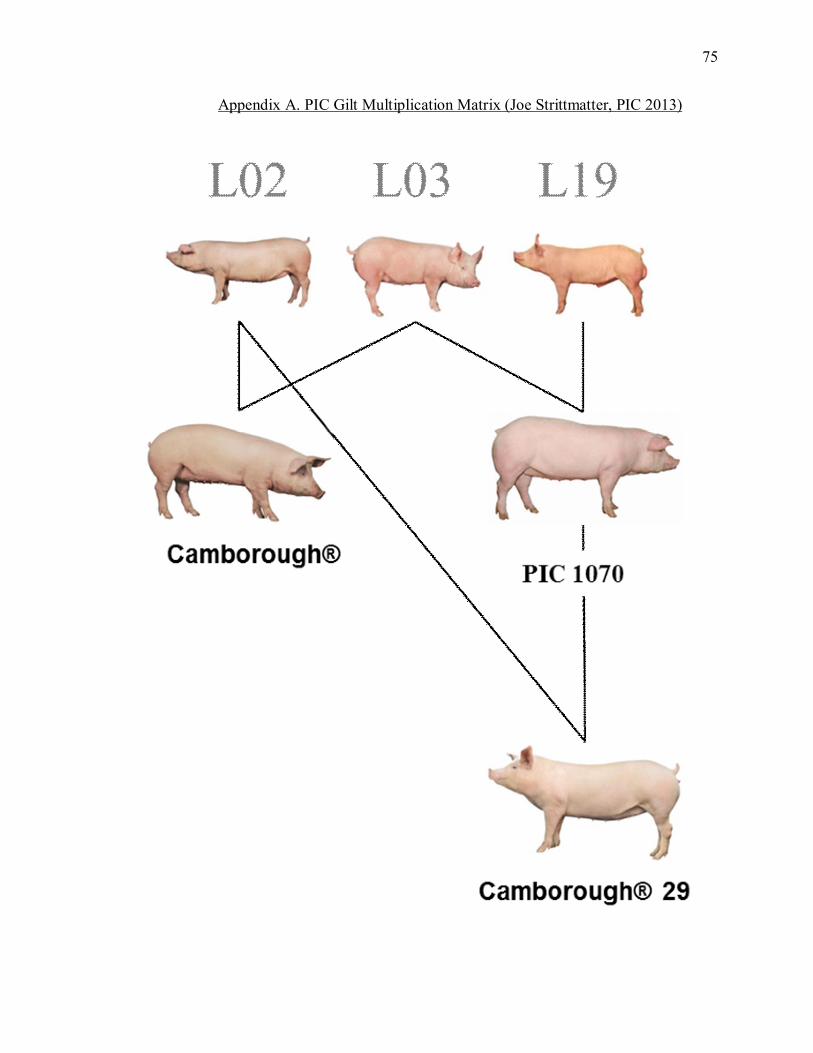
75

Appendix A. PIC Gilt Multiplication Matrix (Joe Strittmatter, PIC 2013)

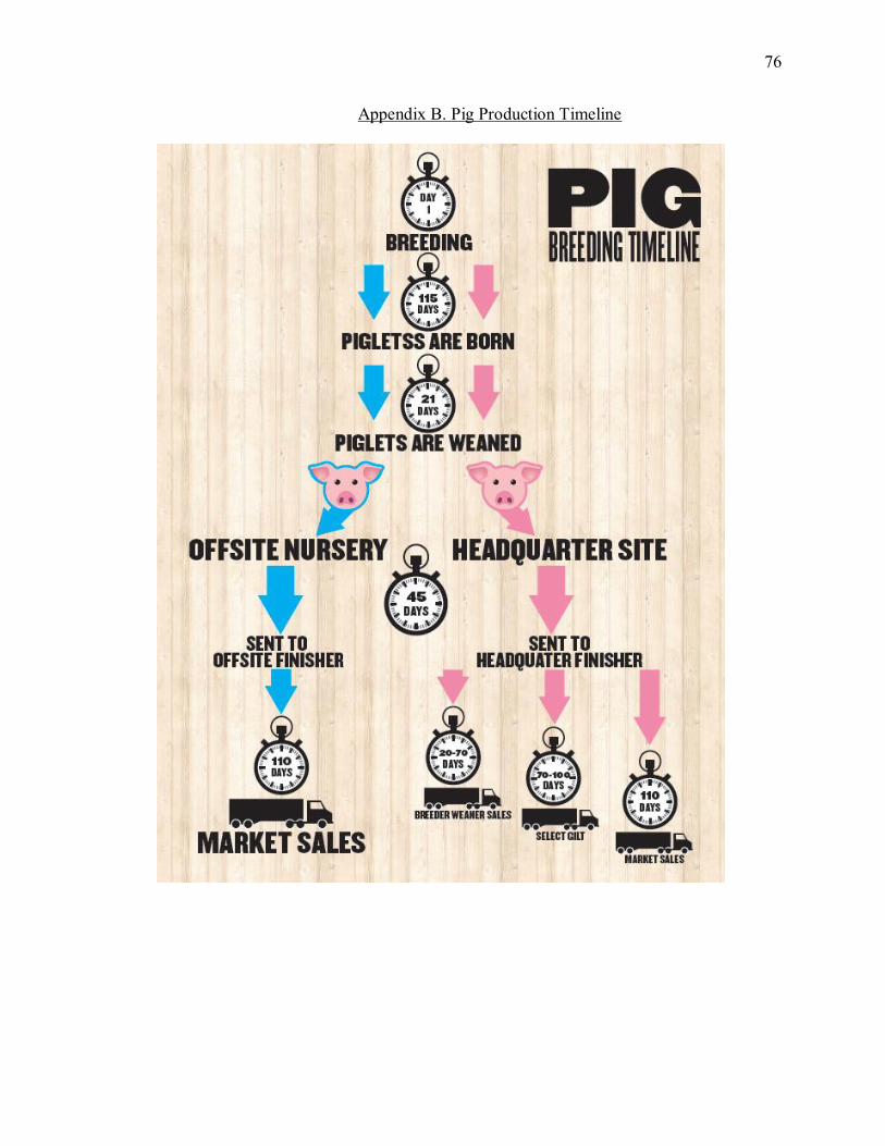
76

Appendix B. Pig Production Timeline

77

Appendix C. Commercial Swine Producer Questionnaire

Commercial Swine Producer Questionnaire with Answers

Please fill out questions applicable to your operation 1) How many total commercial sows do you oversee?

A. 8000 (average) 2) How many separate sow facilities do you manage?

A. 2-3 (average) 3) What is the average number of sows per facility?

A. 2800 4) How many pigs do you finish out in one year?

A. 150,000 (average) 5) How many fulltime people do you employ at each sow unit on average?

A. 10 6) How many fulltime people do you employ total for the finishing pigs?

A. 5 7) How many part-time people do you employ at each sow unit on average?

A. 1 8) How many part-time people do you employ total for the finish pigs?

A. 0 9) For employees with degrees and/or significant work experience, what is the

average hourly wage? A. $15.17/hour

10) For employees without degrees and/or minimal to no experience, what is their average hourly wage?

A. $10.04/hour 11) Do you provide individual health insurance?

A. Yes 12) Do you provide family health insurance?

A. Yes and No 13) Do you provide a retirement savings package?

A. Yes 14) How many hours a week do your employees average a week?

A. 47 15) How much turnover do you see on your operation?

A. 34%

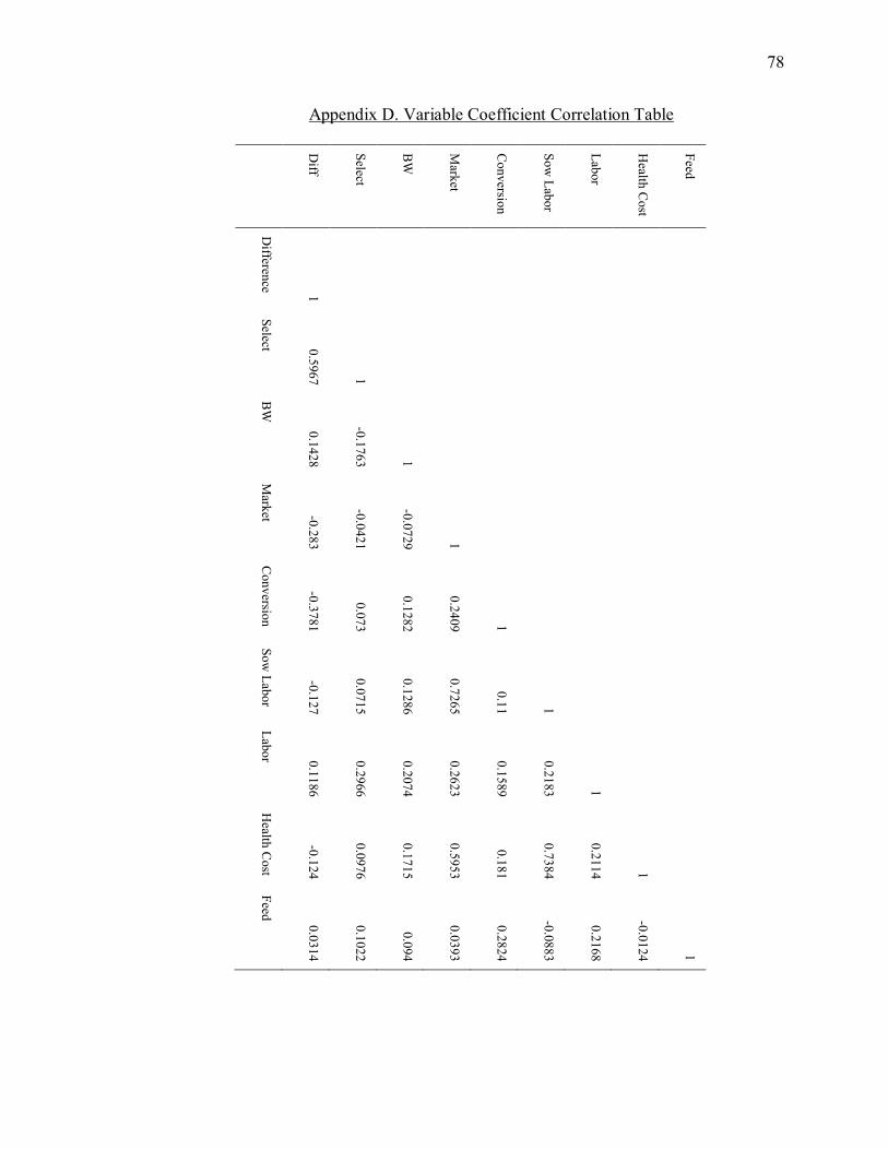
78

Appendix D. Variable Coefficient Correlation Table

Diff

Select

BW

Market

Conversion

Sow Labor

Labor

Health C

ost

Feed

Difference 1

Select 0.5967 1

BW

0.1428

-0.1763 1

Market -0.283

-0.0421

-0.0729 1

Conversion

-0.3781

0.073

0.1282

0.2409 1

Sow Labor

-0.127

0.0715

0.1286

0.7265

0.11 1

Labor 0.1186

0.2966

0.2074

0.2623

0.1589

0.2183 1

Health C

ost

-0.124

0.0976

0.1715

0.5953

0.181

0.7384

0.2114 1

Feed 0.0314

0.1022

0.094

0.0393

0.2824

-0.0883

0.2168

-0.0124 1

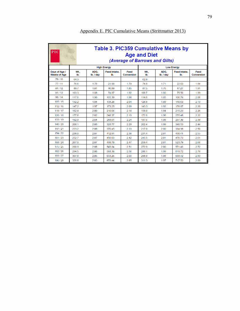
79

Appendix E. PIC Cumulative Means (Strittmatter 2013)

VITA

80

VITA

Nick DeKryger grew up in DeMotte, IN where he spent much of his summers

helping out on the pig farms in production and maintenance. Upon completing his

Bachelor of Science in Biology at Calvin College in Grand Rapids, MI, he took a job for

the National Pork Producers Council, the lobbying arm of the pork industry. After

moving home and completing his Master of Science in Agricultural Economics at Purdue

University, he has accepted a job in marketing and financial analysis at Belstra Milling

Co. in his hometown of DeMotte.