Commercial Imperialism? Political Influence and TradeDuring the Cold War∗

Daniel Berger†

University of Essex

William Easterly‡

New York University and NBER

Nathan Nunn§

Harvard University, NBER, and BREAD

Shanker Satyanath¶

New York University

November 2011

Abstract: We provide evidence that increased political influence, aris-ing from CIA interventions during the Cold War, was used to create alarger foreign market for American products. Following CIA interven-tions, imports from the US increased dramatically, while total exportsto the US were unaffected. The surge in imports was concentratedin industries in which the US had a comparative disadvantage, nota comparative advantage. Our analysis is able to rule out decreasedtrade costs, changing political ideology, and an increase in US loansand grants as alternative explanations. We provide evidence that theincreased imports arose through direct purchases of American prod-ucts by foreign governments.

∗We thank the editor Dirk Krueger and four anonymous referees for comments and suggestions that significantlyimproved the paper. We also thank J. Atsu Amegashie, Scott Baier, Roberto Bonfatti, Richard Chisik, Azim Essaji,Robert Feenstra, Keith Head, Elhanan Helpman, Larry Katz, Tim McKeown, Noel Maurer, Chris Meissner, EdwardMiguel, Kris Mitchener, Marc Muendler, Suresh Naidu, Dani Reiter, Bob Staiger and seminar participants at Columbia,Johns Hopkins SAIS, Stanford, Stellenbosch, UBC, UC Berkeley, UC Davis, Essex, UCLA, UC San Diego, UC SantaCruz, UNC Chapel Hill, USC, Univ. of Pennsylvania, Vanderbilt, NBER DAE and ITI Program Meetings, and theCEA Meetings for valuable comments. We are particularly grateful to Scott Baier for providing the derivation of theBaier-Bergstrand approximation when examining a country’s total imports and total exports. We also thank SayonDeb, Mary Jirmanus, and Eva Ng for excellent research assistance.

†Department of Government, University of Essex. (e-mail: danielsberger@gmail.com).‡Department of Economics, New York University. (e-mail: william.easterly@nyu.edu; website: http://www.nyu.

edu/fas/institute/dri/Easterly/).§Department of Economics, Harvard University. (e-mail: nnunn@fas.harvard.edu; website: http://www.

economics.harvard.edu/faculty/nunn).¶Wilf Family Department of Politics, New York University. (e-mail: shanker.satyanath@nyu.edu; website: http:

//politics.as.nyu.edu/object/ShankerSatyanath.html).

1. Introduction

History provides us with many examples of the use of political power to promote trade and other

national interests, the starkest being the unequal treaties imposed by Western powers on China

and Japan during the 19th and early 20th centuries (Ronald Findlay and Kevin H. O’Rourke, 2007).

However, the general question of whether power is an important determinant of international

trade, particularly in the more recent past, is difficult to examine empirically because shifts in

power relations between governments are often the result of decisions that are made behind the

veil of government secrecy.

In this paper, we surmount this problem by relying on the use of recently declassified CIA doc-

uments to generate a country- and year-specific measure of the influence of the US government

over foreign countries. We identify instances where US covert services engaged in interventions

that installed and/or supported political leaders in other countries. Our interpretation is that

the US government had greater influence over foreign leaders that were installed and supported

by the CIA. Examining the relationship between US influence and annual bilateral trade, we

find that US influence raised the share of total imports that the intervened country purchased

from the US. We find no change in the total value of goods imported from the world. Instead,

increased US influence caused a shift from products produced in other countries and towards US

products. Despite the robust finding of increased imports from the US, we find no evidence that

interventions caused an increase in exports to the US.

These findings are consistent with US political influence being used to create a larger market

for US products in the intervened country. Although we are unable to identify the exact impetus

behind the increase in US exports, it most likely arose from US firms that stood to gain from

increased overseas sales and through standard political economy mechanisms, were able to lobby

the US government.1

Turning to mechanisms, we provide evidence that the increased imports of US products arose

through direct government purchases. We find that the effect of successful interventions on the

purchase of US products is increasing in the government’s share of GDP. For the countries in the

1In theory, it is possible that following a CIA intervention, the intervened-country gains influence over the US. Thiswould be the case if a CIA intervention signals a greater US stake in the survival of the new regime. While, this isvery plausible, our findings of an asymmetric impact on US imports but not US exports, combined with the greaterincrease in US imports in low comparative advantage products (described later), are most consistent with interventionsresulting in greater net influence of the US over the intervened country, rather than vice versa.

1

sample with the smallest government share, we find that the effect of interventions on US imports

is close to zero. This suggests that essentially all of the effect can be explained by government

purchases of US products. We also examine heterogeneous effects across different industries and

find larger impacts in industries in which governments tend to be important purchasers and

importers. We also test for other mechanisms, such as changing tariffs or FDI policies, but find

no evidence that these played an important role.

We recognize that there are many plausible alternative interpretations for these findings. In

addition to the political influence explanation, there are three leading alternative interpretations.

The first is that successful interventions decreased bilateral trading costs between the US and the

intervened country, and this caused an asymmetric increase in trade flows. The second is that the

newly installed and/or supported leaders were ideologically more aligned with Western capitalist

countries. This caused the intervened countries to import more from all Western countries,

including the US. The third explanation is that following a successful intervention, US foreign

aid increased, which caused an increase in the purchase of US products.

We test for the trade costs explanation by examining the effects of CIA interventions on imports

from the US in different industries. We show that the increase in imports from the US was

greatest for goods which the US had a comparative disadvantage in producing. That is, the

new goods that were shipped from the US to the intervened country were products that US

firms were less competitive in producing. This pattern is inconsistent with decreasing trade costs

being the source of increased imports. Standard models of international trade do not predict

greater specialization in comparative disadvantage industries. Instead, integration should cause

each country to specialize (and export more) in industries in which they have a comparative

advantage. The finding is consistent, however, with US influence being used to create a larger

market for products that firms would otherwise have difficulty selling internationally.2

We then turn to the political ideology explanation and test whether the increase in imports

from the US arose because the newly installed regimes were more pro-Western and pro-capitalist

than the previous regimes, and therefore imported more from all Western countries, including

the US. Examining the effects of successful interventions on imports from all countries (not just

from the US), we find that US interventions did not cause an increase in imports from countries

2As discussed, the US government’s desire to increase the overseas sale of these products likely arose through firms’lobbying within the US.

2

that were ideologically similar to the US.

Last, we turn to the increased US loans and grants explanation, testing whether US economic

aid, military aid, or Export-Import Bank loans increased following a successful intervention. We

find that interventions led to an increase in economic aid, military aid, and Export-Import Bank

loans, but that these can only account for, at most, 16% of the total impact of CIA interventions

on imports from the US.

Although our baseline estimating equations control for country-specific time-invariant factors

(with country fixed effects) and time-specific country-invariant factors (with time-period fixed

effects), it is possible that the estimates are biased by omitted factors that simultaneously vary by

time and country. For example, successful CIA interventions may have been more likely following

a temporary decline in imports from the US. This form of selection will result in inflated estimates

of the effect of US influence on imports from the US. We undertake a number of strategies to

control for this, including the use of pre-trends, pre-intervention fixed effects, and controls for

observable characteristics. The results remain robust.

Our analysis of the impacts of CIA interventions links our study to others that also empirically

examine the history of CIA activities during the Cold War. Arindrajit Dube, Ethan Kaplan and

Suresh Naidu (2011) examine the stock prices of US companies in Iran, Guatemala, Cuba, and

Chile before and after the CIA-authorized plans for covert coups. They find that the stock returns

of companies that were both connected to the CIA and stood to gain from the coups increased

immediately after the authorizations. The authors argue that these findings provide evidence

that the top-secret plans were leaked to investors. The focus of our analysis nicely complements

the emphasis of Dube, Kaplan and Naidu (2011). Since the authors are interested in the effects

of top-secret information flows (and not of the interventions themselves), they do not include

the period of the actual intervention in their analysis. In contrast, our analysis looks at the

consequences of the interventions after they are actually carried out. Also related is Daniel Berger,

Alejandro Corvalan, William Easterly and Shanker Satyanath (2010), who use lower frequency

data at five year intervals to examine the effect of interventions on democracy. They find that CIA

and KGB interventions have a negative effect on subsequent democracy.

Our analysis also extends theoretical studies examining the interplay between political influ-

ence and international trade. The hypothesis that influence and power play a role in international

trade dates back to at least Albert O. Hirschman (1945). More recently, the theoretical contribution

3

of Pol Antràs and Gerard Padró-i-Miquel (2011) examines the welfare impacts when political

influence can affect trade and trade policies. Our findings also complement existing studies that

attempt to empirically estimate the effects of political influence on trade flows. An example is

Alexander J. Yeats’ (1990) analysis, showing that among African countries, former colonies pay a

20–30% premium on the price of imported steel when importing from their former colonizer.3

Finally, our findings also contribute to a large literature in political science examining how

political economy factors affect trade. Existing studies, in particular Edward D. Mansfield,

Helen V. Milner and B. Peter Rosendorff (2000, 2002) and Toke S. Aidt and Martin Gassebner

(2010), examine the effects of political regime type (i.e., democratic vs. non-democratic regimes)

on trade flows.4 In contrast to the findings about the extent of democracy in a regime, our findings

show the importance of US influence over foreign regimes arising from CIA interventions.5

The next section of the paper describes the data and their sources and section 3 derives our

estimating equations. Section 4 reports our baseline estimates showing that successful CIA

interventions coincide with increased imports of US goods, no increase in exports to the US,

and no increase in total trade. In section 5, we provide evidence that the increased imports

from the US likely arose through direct government purchases by the newly installed regime. In

section 6, we test for alternative explanations and show that our findings cannot be explained by

decreased trade costs, changing political ideology, or an increase in US loans and grants. Section

7 concludes.

2. Data on Successful CIA Interventions

As a source of variation in US influence over a country, we rely on episodes where the CIA

successfully intervened in foreign countries to either install a new leader or to provide support to

an existing leader to help maintain the power of the regime. To identify these episodes, we rely

3Also related are studies that provide evidence for power and influence playing a role in other international settings.For example, Axel Dreher and Nathan M. Jensen (2007) show that IMF conditionality is correlated with whethercountries vote in-line with the US in the UN General Assembly. Similarly, Christopher Kilby (2009) shows that theWorld Bank’s structural adjustment conditions are less stringent for countries whose voting in the UN is more alignedwith the US. Ilyana Kuziemko and Eric Werker (2006) show that when countries have a seat on the UN security councilthey receive more foreign aid from the US.

4Also see Daniel Verdier (1998), Bruce Russett and John R. Oneal (2001), Timothy Frye and Edward D. Mansfield(2003), Daniel Y. Kono (2006), and Edward D. Mansfield, Helen V. Milner and Jon C. Pevehouse (2008).

5One can interpret our measure of covert CIA interventions as a measure of US “client states” or “puppet leaders”,which are well-established subjects of analysis in the qualitative political science literature (e.g., David Sylvan andStephen Majeski, 2009). Therefore, an alternative interpretation of our analysis is of the effects of US influence onclient states and puppet leaders on trade flows.

4

on studies that document the history of the Cold War, typically based on recently declassified

documents. Using these sources, we construct an annual data set of interventions successfully

undertaken by the CIA. We also construct analogous measures for successful Soviet KGB in-

terventions, which we use as a control in the analysis. The most heavily used sources include

William Blum (2004), Tim Weiner (2007), Odd Arne Westad (2005), Daniel Yergin (1991), and the

Library of Congress’ Country Studies Series for the CIA interventions, and Christopher Andrew

and Vasili Mitrokhin (2000, 2005) for KGB interventions. Full details of the data construction and

sources are reported in a separate data appendix that will be posted on the authors’ web pages

upon publication.

We restrict our analysis to the Cold War period, 1947–1989, because CIA documents for the

post Cold War period largely remain subject to government secrecy. This is the case, in part,

because only classified CIA documents older than 25 years fall under the Freedom of Information

Act, but also because nearly all documents from the Cold War period – even those younger than

25 years – are now publicly available and have been extensively studied and synthesized by Cold

War historians. Once we move beyond 1989 our coding of interventions is based on much less

information and therefore is significantly less certain.6

Our baseline measure of successful CIA interventions is an indicator variable that equals one,

in a country and year, if the CIA either installed a foreign leader or provided covert support for

the regime once in power. We label this variable US influencet,c. The activities used by the CIA

to install and help maintain the power of specific regimes are many and varied. They include

the creation and dissemination of (often false) propaganda, usually through radio, television,

newspapers and pamphlets. They also included covert political operations, which typically

consisted of the provision of funds and expertise for political campaigns. More invasive tactics

included the destruction of physical infrastructure and capital, as well as covert paramilitary

operations, that included the supply of arms and military equipment, direct involvement in

insurgency and counterinsurgency operations, and the coordination of coups and assassinations

(Loch K. Johnson, 1989, 1992).7

6An additional benefit of examining only the Cold War era is that there is greater comparability over time, so thatour coefficient estimates are likely more stable across the years of our sample. This is less likely to be true once wepool the Cold War and the post-Cold War periods.

7Our analysis does not distinguish between different types of intervention episodes. It is possible that the impactof CIA interventions on trade is heterogeneous, depending on specific characteristics of an intervention. Our analysisdoes not examine this potential heterogeneity, but instead simply examines the average effect across all interventions.

5

There are many instances in which the CIA set out to remove an existing leader and install

a new leader in power. The CIA-organized coups in Iran in 1953, Guatemala in 1954, and Chile

in 1973 are the most well-known examples of such cases. For these interventions, the indicator

variable US influencet,c takes on the value of one. In other cases, the CIA began to provide support

for leaders currently in power. In these cases, the CIA did not engage in activities to install

the leader into power, but once in power, at some point, the CIA began to engage in activities

to help maintain the power of the regime. Typically, these were covert counter-insurgency

operations undertaken by the CIA. We also code as one these cases in which the leader maintains

power with the help of the CIA.8 As a robustness check, we disaggregate our baseline indicator

variable, distinguishing between intervention episodes that installed and then supported a leader

and episodes that propped up existing leaders. We find that both types of interventions have

quantitatively similar impacts.

As a concrete illustration of the construction of our variable, we use the history of the CIA in

Chile. CIA involvement in Chile first occurred in the 1964 Presidential election, when the CIA

provided covert funding and support for the Christian Democratic Party candidate Eduardo Frei

Montalvo. Eduardo Frei won the election and continued to receive CIA support while he was in

power. In the 1970 election, Salvador Allende, a candidate from a coalition of leftist parties, was

elected, and remained in power until the famous CIA orchestrated coup of 1973. After the coup,

Augusto Pinochet took power and was backed by the CIA until 1988. Since our indicator for

successful CIA interventions, US influencet,c, equals one in all years in which a leader is installed

or supported by the CIA, for Chile the variable equals one from 1964 to 1970 when Eduardo Frei

was in power. It equals zero in 1971 and 1972, the years when Salvador Allende was in office

(since he was not installed or supported by the CIA). It then equals one from 1973 to 1988, the

years when Augusto Pinochet, who was installed and supported by the CIA, was in power.9

Our empirical analysis examines a sample of 166 countries, which includes all countries for

8 A good example of this is the CIA’s involvement in Haiti. Paul Magloire, François “Papa Doc” Duvalier, andJean-Claude “Baby Doc” Duvalier, were not installed by the CIA, but they were reliant on CIA support to help maintaintheir power.

9A potential source of imprecision arises from the fact that our data are measured at annual frequencies, while inreality CIA activities occurred in continuous time. This results in some imprecision when coding US influencet,c. Forthe case of Chile, since Salvador Allende won the election on September 4, 1970, it is unclear whether we should codeUS influencet,c as one or zero for in 1970. In constructing our measure we code onset and offset years as being anintervention year. Therefore, since 1970 is an offset year of the CIA’s support of Eduardo Frei, it is coded as one. Wehave checked that none of our results depend on this decision. Choosing instead to code onset- and offset-interventionyears as zero yields results that are virtually identical to what we report here.

6

which necessary data are available, except the United States and the Soviet Union.10 Among

the 166 countries, 51 were subject to at least one CIA intervention between 1947 and 1989.11

In an average year between 1947 and 1989, 25 countries were experiencing a CIA intervention.

Among the group of countries that experienced an intervention between 1947 and 1989, the typical

country experienced 21 years of interventions.

Examining the total number of successful CIA interventions in each year, we find that there is

a steady increase after 1947 until the 1970s, after which the number falls until 1989.12 This pattern

is consistent with the known history of the CIA. Between 1953 and 1961 covert action increased

significantly, with attention focused on political action, particularly support to political figures

and political parties. The 1960s witnessed a continued presence of CIA covert activities, although

there was a shift towards greater paramilitary activities. The period from 1964 to 1967 is known

to have been the high point of CIA covert activities, with the post-1967 slow-down brought about,

in part, by the 1967 Ramparts magazine article that exposed the CIA’s funding of national student

groups and other private organizations (William M. Leary, 1984). Consistent with history, our

data show a leveling off of covert interventions in the late 1960s until the mid-1970s, after which

the number falls.13

The map shown in figure 1 reports for each country the fraction of years between 1947 and

1989 for which there was a CIA intervention.14 The cross-country distribution of interventions is

consistent with the descriptive history of CIA activities during the Cold War. The CIA intervened

most heavily in Latin America, but also in a few European countries – namely, Italy and Greece –

as well as in a number of countries in Africa, Asia, and the Middle East.

The map also helps to illustrate exactly what our intervention variable captures and what it

does not capture. For example, our intervention variable is zero for Angola throughout the period.

This is so despite the heavy and well-known involvement of the CIA in Angola’s civil war, where

they provided covert support for the anticommunist group Union for the Total Independence of

10Our panel is unbalanced, since countries do not enter the sample until they gain independence. Countries thatsplit or merge are treated as new countries in the data set. A description of how exactly we deal with these cases isprovided in an online appendix.

11Similarly, 25 countries were subject to at least one successful KGB intervention.12See figure A1 of the online appendix for details.13The slight lag in the decline after 1967 results from the persistence of ongoing intervention episodes, since newly

installed or newly supported leaders were often supported by the CIA for their remaining tenure.14For countries that did not gain independence until after 1947, we report the fraction of years from independence

to 1989 for which there was a CIA intervention.

7

Year

s with

US i

nflue

nce =

1Pr

opor

tion,

1947

-1989

0-1

%

1-10%

20

-40%

40

-60%

60

-80%

80

-100%

No

t in sa

mple

Figu

re1:

Map

show

ing

the

frac

tion

ofye

ars

betw

een

1947

and

1989

wit

ha

CIA

inte

rven

tion

.

8

Angola (UNITA) (e.g. Stephen R. Weissman, 1979). However, the group was never successful

at gaining power from the Movimento Popular de Libertação de Angola (MPLA). Because the

US-backed UNITA forces never gained control of the government, our variable is not coded as

one for Angola, despite clear involvement by the CIA in the country. The example illustrates that

our intervention measure is not a measure of all CIA meddling or activities in a country. Rather,

it is an indicator of CIA activities that were successful at either installing a new leader or in

maintaining the power of an existing leader. Therefore, it should be kept in mind that throughout

the paper, when we refer to “CIA interventions”, we are referring specifically to interventions by

the CIA that were successful at installing or maintaining the power of specific leaders.

Using CIA covert activities to measure changes in US influence over foreign countries has a

number of particularly attractive characteristics. First, because these interventions were covert

at the time, they were largely unaffected by US public opinion, and from the opinion of other

countries in the international arena, which reduces one source of endogeneity in our measure.15

Further, because the interventions affect the leader in power, they are significant and potentially

have an important impact on US government influence over the regime.

Our analysis also relies on trade data from the Correlates of War (COW) Trade Dataset (Kather-

ine Barbieri, Omar M.G. Keshk and Brian M. Pollins, 2008), which reports annual aggregate

bilateral trade flows (measured in millions of nominal US dollars).16 All other data from our

analysis are described as they are used.

3. Estimating Equations

Our estimating equations are based on the gravity model of international trade, which has become

the conventional framework for estimating the determinants of trade flows. The gravity model

can be derived formally from a number of theoretical environments. Consider, for example, the

15The findings from Dube, Kaplan and Naidu (2011) suggest a potentially important caveat here. The authorsprovide evidence that US special interests were informed about CIA-planned coups. Specifically, they show that thestock prices of multinational corporations that stood to gain from the coups responded after top secret authorizationswere made. In fact, stock prices responded more to these authorizations than to the actual coups themselves. Thesefindings suggests that while the general public was uninformed about covert CIA actions at the time, this may nothave been true for an informed subset of the population that was politically connected.

16For the post WWII period, the data are originally from the International Monetary Fund’s Direction of TradeStatistics. Exploiting the fact that all transactions are potentially recorded by both importing and exporting countries,Barbieri, Keshk and Pollins impute missing flows by using, for example, the exporter’s trade statistics if data onimports are missing from the importer’s accounts. Because importing countries typically keep more precise records ofshipments (because of the existence of tariffs) than exporting countries, the dataset uses importing country accountswhen both sources exist. A full discussion is provided in Barbieri, Keshk and Pollins (2008) and Katherine Barbieri,Omar M.G. Keshk and Brian M. Pollins (2009). In particular, see table 1 of Barbieri, Keshk and Pollins (2009).

9

setting from James Anderson and Eric van Wincoop (2003).17 Here, trade between country c and

e in year t is given by:

mt,c,e =Yt,cYt,e

Y Wt

[τt,c,ePt,cPt,e

]1−σ(1)

where mt,c,e denotes imports into country c from exporter e in year t, Yt,c is total GDP of importing

country c in year t, Yt,e is total GDP of exporting country e in year t, and Y Wt is world GDP in

year t. The parameter σ is the elasticity of substitution between goods, τt,c,e measures bilateral

trade related costs when shipping goods from country e to c, and Pt,c and Pt,e are multilateral

resistance terms for countries c and e, respectively, which are complex non-linear functions of the

full set of bilateral cost terms τt,c,e.18

Taking natural logs and rearranging gives:

lnmt,c,e

Yt,cYt,e= − lnY W

t + (1− σ) ln τt,c,e − (1− σ)[lnPt,c + lnPt,e] (2)

Estimating equation (2) faces the challenge of accounting for the importer and exporter multilat-

eral resistance terms, Pt,c and Pt,e. We follow the estimation method proposed by Scott L. Baier

and Jeffrey H. Bergstrand (2009), where the term is approximated using a first-order log-linear

Taylor series expansion. Baier and Bergstrand characterize the resulting approximation terms and

show that the technique generates estimates that are virtually identical to the nonlinear estimation

of the full system of equations proposed by Anderson and van Wincoop (2003).

Baier and Bergstrand (2009) show (see, in particular, section 3 and appendix A of their paper)

that with the assumption of symmetry, the multilateral resistance terms are given by:

lnPt,c =N

∑i=1

θt,i ln τt,c,i −12

N

∑k=1

N

∑m=1

θt,kθt,m ln τt,k,m

lnPt,e =N

∑j=1

θt,j ln τt,j,e −12

N

∑k=1

N

∑m=1

θt,kθt,m ln τt,k,m

where θt,i ≡ Yt,i/Y Wt . The sum of the two multilateral resistance terms is given by:

lnPt,c + lnPt,e =N

∑i=1

θt,i ln τt,c,i +N

∑j=1

θt,j ln τt,j,e −N

∑k=1

N

∑m=1

θt,kθt,m ln τt,k,m (3)

We assume that bilateral trade costs are given by

τt,c,e ≡ eµ1 ln distc,e+µ2Ilangc,e +µ3I

borderc,e +µ4I

gattt,c,e+µ5,Irta

t,c,e (4)

17Alternative foundations are provided by Jonathan Eaton and Samuel Kortum (2002) and Thomas Chaney (2008).18See equation (12) of Anderson and van Wincoop (2003) for the derivation and a general discussion.

10

where ln distc,e is the natural log of the distance between country e and c, I langc,e is an indicator

variable that equals one if the two countries share a common language, Iborderc,e is an indicator for

the two countries sharing a border, Igattt,c,e is an indicator that equals one if both countries are GATT

participants in year t, and Irtat,c,e equals one if both countries belong to a regional trade agreement

in year t.19 Substituting equation (4) into (3) gives:

lnPt,c + lnPt,e = µ1Xdistc,e + µ2X

langc,e + µ3X

borderc,e + µ4X

gattt,c,e + µ5X

rtat,c,e (5)

where

Xdistc,e ≡

N

∑i=1

θt,i ln distc,i +N

∑j=1

θt,j ln distj,e −N

∑k=1

N

∑m=1

θt,kθt,m ln distk,m

X lc,e ≡

N

∑i=1

θt,iIlc,i +

N

∑j=1

θt,jIlj,e −

N

∑k=1

N

∑m=1

θt,kθt,mIlk,m for l = lang, border

X lt,c,e ≡

N

∑i=1

θt,iIlt,c,i +

N

∑j=1

θt,jIlt,j,e −

N

∑k=1

N

∑m=1

θt,kθt,mIlt,k,m for l = gatt, rta

One can then use the observable variables given in equations (4) and (5) to control for trade

costs τt,c,e and the multilateral resistance terms [lnPt,c + lnPt,e] that appear in equation (2).

The primary impact of interest is how increased US influence, through CIA interventions,

affected trade with the US. Therefore, our baseline estimating equation examines the impact of

a CIA intervention in country c on country c’s trade with the US.20 Consider first country c’s

imports from the US, which we denote mUSt,c . This can be expressed as:

mUSt,c =

Yt,cYUSt

Y Wt

[τUSt,c

Pt,cPUSt

]1−σ

where Y USt denotes US total income, PUS

t denotes the multilateral resistance term for the US, and

τUSt,c is the trade friction between the US and country c. Taking natural logs and rearranging gives:

lnmUSt,c

Yt,c= ln

Y USt

Y Wt

+ (1− σ) ln τUSt,c − (1− σ)[lnPUS

t + lnPt,c] (6)

19Distances are calculated manually as the great circle distance between the centroid of each country. Data ontrading partner’s with common language, with contiguous borders, and belonging to a regional trade agreement arefrom Keith Head, Thierry Mayer and John Ries (2010). Data on GATT participation are from Michael Tomz, Judith L.Goldstein and Douglas Rivers (2007).

20An alternative estimation strategy is to examine bilateral trade between all countries and examine how CIAinterventions differentially impacted a country’s trade with the US (relative to its trade with all other countries).As we report in section 6B, this generates estimates that are very similar to our baseline strategy. A disadvantage ofa full bilateral analysis is that, even with clustered standard errors, one runs the risk of generating downward-biasedstandard errors (see Marianne Bertrand, Esther Duflo and Sendhil Mullainathan, 2004, Robert S. Erikson, Pablo M.Pinto and Kelly T. Rader, 2009). Our baseline strategy has only N × T observations rather than the N(N − 1)Tobservations in the bilateral sample (where N is the number of countries and T is the number of time periods).

11

Our analysis is interested in identifying the reduced-form impact of US influence on a coun-

try’s trade with the US. Because it is possible that some of the mechanisms underlying this

relationship lie outside of the standard gravity model of international trade, we estimate equation

(6) and include CIA interventions as an additional determinant of trade flows, thus estimating

the reduced-form relationship between CIA interventions and imports from the US:

lnmUSt,c

Yt,c= αt + αc + βUS influencet,c + φ ln τUSt,c − φ[lnPUSt + lnPt,c] + Xt,cΓ + εt,c (7)

The dependent variable, ln mUSt,c

Yt,c, is the natural log of imports into country c from the US normal-

ized by country c total GDP.21 Our primary coefficient of interest is β, which captures the average

reduced-form impact of CIA interventions on the countries that experience an intervention.22

The first terms in equation (6), ln Y USt

YWt

, is absorbed by the year fixed effects αt in equation

(7). Trade costs, ln τUSt,c , are controlled for with the observables given in equation (4) and the

multilateral resistance terms, [Pt,c + PUSt ], are controlled using the observable terms given in

equation (5). Guided by the theory, in equation (7), the coefficients for ln τUSt,c and [Pt,c+PUSt ] are

constrained to have the same coefficients but with opposite signs.

Equation (7) also includes country fixed effects, αc, which capture time-invariant country

characteristics that may be correlated with both trade with the US and CIA interventions. We

also control for a vector of time-varying control variables Xt,c, which includes the natural log of

per capita income and an indicator for Soviet/KGB interventions, measured in the same manner

as CIA interventions. Motivated by recent studies showing that leaders matter (e.g., Benjamin

Jones and Benjamin Olken, 2005, 2009), we control for an indicator variable that equals one if

there is a change in leadership, as well as a measure of the tenure of the current leader. Our final

control variable is motivated by the findings from Berger et al. (2010), showing that successful

CIA interventions adversely impacted democracy. We control for an indicator variable that equals

one if an observation is a democracy, as defined by José Antonio Cheibub, Jennifer Gandhi and

21Trade and income are both measured in millions of nominal US dollars.22Because we use an indicator variable that captures the existence of all interventions, without distinguishing

between intensity or type, our estimate does not identify heterogeneous impacts which may underly the averageeffect. We have tested for temporal and spatial heterogeneity. We find some evidence of heterogeneous impacts. Forexample, we find that the impact of CIA interventions is greater than average in the 1950s and weaker than average inthe 1970s. We also find evidence of a weaker effect among African countries. These results are reported in an onlineappendix.

12

James Raymond Vreeland (2010).23

In auxiliary regressions, we also examine the effect of CIA interventions on exports to the US.

The estimating equation for exports is derived in an analogous manner as equation (7) and is

given by:

lnxUSt,c

Yt,c= αt + αc + βUS influencet,c + φ ln τUSt,c − φ[lnPUSt + lnPt,c] + Xt,cΓ + εt,c (8)

where c now indexes exporters and xUSt,c denotes the values of exports from country c to the US.

4. Baseline Estimation Results

We now turn to our estimation results, which are reported in table 1. Column 1 reports estimates

of equation (7) without controlling for the multilateral resistance terms. The equation does,

however, include country fixed effects and year fixed effects. We find that the coefficient on

the US intervention measure, US influencet,c, is positive and statistically significant. The estimated

coefficient of 0.293 implies that in intervention years a country’s trade with the US is 29.3 percent

greater than in non-intervention years. This is a sizable impact.

In column 2, we do not control for country fixed effects but do control for countries’ multilat-

eral resistance terms using the Baier and Bergstrand (2009) approximation method described in

the previous section. The estimated impact is much larger with a coefficient of 0.778. In column 3,

we include both the Baier and Bergstrand multilateral resistance terms and country fixed effects.

The estimated coefficient is 0.303. The relative magnitudes of the coefficients from columns 1–3

show the importance of controlling for country fixed effects. When these are not included in

the table, the estimated impact of CIA interventions are over twice as large. This suggests

the existence of time-invariant country characteristics that if not properly taken into account

generate an upwards bias in our coefficients of interest. As well, once country fixed effects are

accounted for, additionally controlling for the Baier and Bergstrand multilateral resistance terms

has no noticeable impact on our estimate of interest β. This most likely reflects the fact that a

country’s multilateral resistance term typically does not change drastically from one year to the

next. Therefore, most of the variation in the term is in the cross section and is captured to a large

23Using the Polity measure of democracy yields virtually identical estimates to what we report here. Unlike thePolity measure, which is based on subjective perceptions about the extent of democracy, the Cheibub, Gandhi andVreeland (2010) measure is based on objective criteria about the extent to which government positions are filled bycontested elections (see e.g., Mike Alvarez, José Antonio Cheibub, Fernando Limongi and Adam Przeworski, 1996).

13

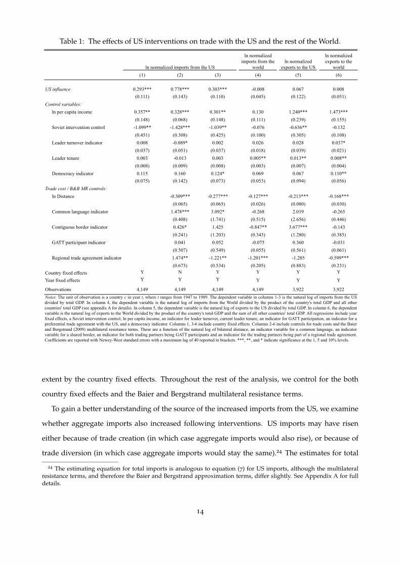
Table 1: The effects of US interventions on trade with the US and the rest of the World.

(1) (2) (3) (4) (5) (6)

US influence 0.293*** 0.778*** 0.303*** -0.008 0.067 0.008(0.111) (0.143) (0.110) (0.045) (0.122) (0.051)

Control variables:ln per capita income 0.357** 0.328*** 0.301** 0.130 1.240*** 1.473***

(0.148) (0.068) (0.148) (0.111) (0.239) (0.155)Soviet intervention control -1.099** -1.428*** -1.039** -0.076 -0.636** -0.132

(0.451) (0.308) (0.425) (0.100) (0.305) (0.108)Leader turnover indicator 0.008 -0.089* 0.002 0.026 0.028 0.037*

(0.037) (0.051) (0.037) (0.018) (0.039) (0.021)Leader tenure 0.003 -0.013 0.003 0.005** 0.013** 0.008**

(0.008) (0.009) (0.008) (0.003) (0.007) (0.004)Democracy indicator 0.115 0.160 0.124* 0.069 0.067 0.110**

(0.075) (0.142) (0.073) (0.053) (0.094) (0.056)Trade cost / B&B MR controls:

ln Distance -0.309*** -0.277*** -0.127*** -0.213*** -0.168***(0.065) (0.065) (0.026) (0.080) (0.030)

Common language indicator 1.478*** 3.092* -0.268 2.019 -0.265(0.408) (1.741) (0.515) (2.656) (0.446)

Contiguous border indicator 0.426* 1.425 -0.847** 3.677*** -0.143(0.241) (1.203) (0.343) (1.280) (0.385)

GATT participant indicator 0.041 0.052 -0.075 0.360 -0.031(0.507) (0.549) (0.055) (0.561) (0.061)

Regional trade agreement indicator 1.474** -1.221** -1.201*** -1.285 -0.599***(0.673) (0.534) (0.205) (0.883) (0.231)

Country fixed effects Y N Y Y Y Y

Year fixed effects Y Y Y Y Y Y

Observations 4,149 4,149 4,149 4,149 3,922 3,922

ln normalized imports from the US

ln normalized imports from the

worldln normalized

exports to the US

ln normalized exports to the

world

Notes: The unit of observation is a country c in year t, where t ranges from 1947 to 1989. The dependent variable in columns 1-3 is the natural log of imports from the USdivided by total GDP. In column 4, the dependent variable is the natural log of imports from the World divided by the product of the country's total GDP and all othercountries' total GDP (see appendix A for details). In column 5, the dependent variable is the natural log of exports to the US divided by total GDP. In column 6, the dependentvariable is the natural log of exports to the World divided by the product of the country's total GDP and the sum of all other countries' total GDP. All regressions include yearfixed effects, a Soviet intervention control, ln per capita income, an indicator for leader turnover, current leader tenure, an indicator for GATT participation, an indicator for apreferential trade agreement with the US, and a democracy indicator. Columns 1, 3-6 include country fixed effects. Columns 2-6 include controls for trade costs and the Baierand Bergstrand (2009) multilateral resistance terms. These are a function of the natural log of bilateral distance, an indicator variable for a common language, an indicatorvariable for a shared border, an indicator for both trading partners being GATT participants and an indicator for the trading partners being part of a regional trade agreement.Coefficients are reported with Newey-West standard errors with a maximum lag of 40 reported in brackets. ***, **, and * indicate significance at the 1, 5 and 10% levels.

extent by the country fixed effects. Throughout the rest of the analysis, we control for the both

country fixed effects and the Baier and Bergstrand multilateral resistance terms.

To gain a better understanding of the source of the increased imports from the US, we examine

whether aggregate imports also increased following interventions. US imports may have risen

either because of trade creation (in which case aggregate imports would also rise), or because of

trade diversion (in which case aggregate imports would stay the same).24 The estimates for total

24 The estimating equation for total imports is analogous to equation (7) for US imports, although the multilateralresistance terms, and therefore the Baier and Bergstrand approximation terms, differ slightly. See Appendix A for fulldetails.

14

imports, reported in column 4, show that the impact of interventions on aggregate imports is not

statistically different from zero. Further, this is the result of a small coefficient that is precisely

estimated and not because of large standard errors. This suggests that the increased share of

imports from the US arose from a shift away from imports from other countries and towards

imports from the US. We confirm this finding in our bilateral regression analysis reported in

section 6B, where we explicitly estimate the trade-diversion impact of CIA interventions.

We next ask whether intervened countries also experienced an increase in their exports to the

US. Column 5 reports estimates of equation (8). The results show that, unlike US imports, exports

to the US were not affected by CIA interventions. In column 6, for completeness, we report

estimates of the impact of US. interventions on aggregate exports.25 We find that interventions

had no effect on aggregate exports.

Table 1 also reports the coefficient estimates for all additional control variables. These are

generally as expected. Soviet interventions tend to decrease trade with the US and countries with

greater per capita income tend to import and export more from all countries, including the US.

We find no evidence that leader turnover or leader tenure systematically affect imports from the

US. Of the trade cost variables, bilateral distance significantly reduces trade, but the other trade

cost variables are less robust, a fact most likely explained by collinearity with the country fixed

effects. To conserve on space, in the remaining tables of the paper, we suppress the coefficient

estimates of the control variables. These are available upon request.

Although our estimating equation controls for country-specific time-invariant factors and

time-specific country-invariant factors that could bias our estimates of interest, there remains the

concern that our coefficient of interest β may be biased due to factors that vary simultaneously

by country and time period. The primary concern is that there may have been selection in the

targeting of CIA interventions and, in particular, that interventions were more common when a

country had recently experienced a decline in its imports of US products. This is an example of

the well-known “Ashenfelter dip”.

We undertake a number of strategies to reduce any potential bias that may arise from the

endogeneity of interventions. We control for five year pre-trends in the dependent variable (i.e.,

lnmUSt−1,c − lnmUS

t−6,c), which capture potential pre-intervention ‘dips’ in imports. We also control

for an indicator variable that equals one if the observation (country c in period t) is between 1 and

25See Appendix A for details about the estimating equation for total exports.

15

5 years prior to the onset of an intervention episode. With either strategy, we obtain estimates of

β that are very similar to our baseline estimate (see columns 1 and 2 of appendix table A6).26

We also check that our results are robust to controlling for potentially important observable

factors, like the nature of a country’s foreign relations with the US and economic conditions in the

foreign country (columns 3 and 4 of appendix table A6). The foreign relations variables include

three indicator variables that identify instances in which either the foreign country or the US

threatens to use force, displays force, or uses force; an indicator variable that equals one if there

are US sanctions against exporting to the country; and an indicator variable that equals one if

the country has an alliance with the US. The economic condition variables, which we include

in addition to our baseline control of per capita income, are the one-year average inflation rate

(between period t− 1 and t) and the real exchange rate.27

The final causality test that we perform examines the timing of movements in US imports just

before and after the beginning of an intervention episode. This is done by controlling for five

indicator variables, each of which equals one in one of the five years prior to an intervention

onset, and five indicator variables for the five years immediately after the onset year. We find that

even controlling for these leads and lags, interventions continue to have a positive and statistically

significant impact on US imports.28 We also find that all of the estimated lead and lag coefficients

are statistically insignificant, which shows that there is no systematic change in US imports prior

to the onset of an intervention, and that there is no movement in US imports in the years following

an onset that is not accounted for by the intervention. Full estimates are reported in appendix

table A7.

We also perform a number of sensitivity tests. Since our estimating equations are derived

from a log-linearization of the gravity model, a small of number zero trade observations (139 of

4,288) are dropped from the sample. We check that our results remain robust when estimating

equation (7) using a Poisson pseudo maximum likelihood estimator, as suggested by J.M.C.

26 This robustness is consistent with historical accounts that emphasize the primarily ideological motivation – namelythe fear of Communism – behind CIA interventions (e.g., Westad, 2005, p. 111; Blum, 2004, p. 13). Although economicconsiderations did play a role – particularly when the foreign country’s movement towards communism or socialismmeant nationalizing foreign companies – they do not appear to have been the most important motivation.

27The military dispute data are from Zeev Maoz (2005), the sanctions data are from Gary Clyde Hufbauer, Jeffrey J.Schott, Kimberly Ann Elliott and Barbara Oegg (2009), the alliance data are from the COW Alliance Dataset 3.03, andthe inflation and exchange rate data are from the Penn World Tables 6.3.

28We find that the estimated impact for the onset year is smaller than for subsequent years. This is explained by thefact that because of the way we construct our intervention variable, the onset year only experiences an intervention inpart of the calendar year. In other words, in onset years the country is only partially treated by the CIA interventionand therefore we would expect a smaller coefficient in this year.

16

Santos Silva and Silvana Tenreyro (2006) (column 5 of appendix table A6). Motivated by the

observed persistence of trade flows, potentially due to hysteresis arising from the fixed costs of

exporting, we also check that we obtain similar estimates when we controls for a one-year lag of

the dependent variable (columns 6–8 of appendix table A7).

Our final sensitivity check distinguishes between intervention episodes that began with the

CIA installing a new leader and then providing support for the leader and episodes in which the

CIA began supporting a pre-existing leader. We disaggregate US influencet,c into two measures:

an indicator variable that equals one for interventions of the first type (install and support) and

the second is an indicator variable that equals one for interventions of the second type (support

only).29 We find that both types of interventions have very similar impacts (column 9 of table

A6).

5. Underlying Mechanisms

Turning to mechanisms, we now provide evidence that much of the increase in imports from the

US likely arose through direct government purchases.

Quantitively speaking, the purchase of goods by governments would be large enough to

account for the CIA intervention induced increases in imports from the US observed in the

data.30 In addition, it is well-known that government purchases are highly discriminatory, with

suppliers typically based on criteria other than lowest costs (Baldwin, 1970, Thomas C. Lowinger,

1976, Audet, 2002), and that influence, power and connections are important factors that affect

governments’ choice of suppliers (Federico Cingano and Paolo Pinotti, 2010, Eitan Goldman, Jorg

Rocholl and Jongil So, 2008).

29In the sample, there are 933 country-year observations with an intervention. Of these, 362 interventions are‘install and support’ interventions and 571 are ‘support only’ interventions. Of the 51 countries that experienced anintervention, 27 experienced ‘install and support’ interventions, 19 experienced ‘support only’, and 5 experienced anintervention episode of each type.

30 As a share of GDP, government purchases have typically been around 20 percent for industrialized nations and15 percent for developing nations (Robert E. Baldwin, 1970, p. 58, Denis Audet, 2002). Removing compensation toemployees and focusing only on purchases of goods, the figures become 10.3 and 8.8%, respectively (Audet, 2002).These figures can be compared to the predicted intervention-induced increase in imports based on our estimates. Themean of US imports relative to total GDP in the sample is 0.002 or 0.2%. (For the observation in the 90th percentile thefigure is still only 0.060 or 6%.) According to the estimate from column 3 of table 1, interventions increase US imports(as a share of GDP) by 30.3 percent. Therefore, for a country initially at the mean US import-to-GDP ratio, US importsrelative to GDP would increase from 0.20% to 0.26%. For a country at the 90th percentile, the increase would be from6.0% to 7.8%. Therefore, the predicted increase in imports can be fully accounted for by government purchases, giventhat the average share of government purchases to GDP approximately 9–10%.

17

Table 2: Causal Mechanisms.

(1) (2) (3) (4) (5)

US influence 0.246** 0.001 0.0121 0.246*** 0.261***(0.113) (0.165) (0.166) (0.081) (0.079)

US influence x Govt share of GDP 1.355*** 1.318**(0.519) (0.514)

US influence x IHigh Govt Purchases 0.176**(0.074)

US influence x IHigh Govt Imports 0.141**(0.072)

Govt share of GDP N Y Y N NGovt share of GDP x All controls N N Y N N

Observations 3,710 3,710 3,710 142,243 142,243Notes: In columns 1-3,the unit of observation is a country c, in year t, where t ranges from 1947 to 1989. In columns 4-5, the unit ofobservation is a country c, in year t, in a 2-digit SITC industry i, where t ranges from 1962 to 1989. The dependent variable is the natural log ofthe imports from the US divided by total GDP. All regressions include year fixed effects, country fixed effects, a Soviet intervention control, lnper capita income, an indicator for leader turnover, current leader tenure, a democracy indicator, as well as Baier and Bergstrand (2009)controls for trade costs and multilateral resistance terms. These are a function of the natural log of bilateral distance, an indicator variable for acommon language, an indicator variable for a shared border, an indicator for both trading partners being GATT participants and an indicator forthe trading partners being part of a regional trade agreement. Columns 4-5 also include industry fixed effects. Coefficients are reported withNewey-West standard errors in brackets in columns 1-3 and with standard errors clustered at the country-year level in brackets in columns 4-5.***, **, and * indicate significance at the 1, 5 and 10% levels.

Dependent variable: ln normalized imports US

Country-year level Country-year-industry level

We test for the government-procurement channel by examining whether the estimated impact

of CIA interventions on US imports is greater in countries where the government controls a

greater share of the economy, which we measure using the share of government expenditures in

GDP, taken from the Penn World Tables 6.3. Estimation results are reported in columns 1–3 of

table 2. Column 1 reproduces the baseline estimate from column 3 of table 1, but with a smaller

sample size due to missing government expenditure data.31 Column 2 reports estimates of a

specification that allows the effect of CIA interventions to differ depending on the government’s

share of GDP. As shown, the interaction between US influencet,c and the government expenditure

share is positive and statistically significant.

The magnitudes of the estimates suggest significant heterogeneity across observations. To

see this, first note that the government expenditure shares for observations at the 10th, and

90th percentiles are .077 (i.e. 7.7%) and .277. According to the estimates the effect of CIA

interventions on observations between the 10th and 90th percentiles range from .105 to .376.32

31Data on government expenditure share are unavailable for all countries, and are only available from 1950.32The effects for each percentile are calculated as follows: .001 + (.077× 1.355) = .105 and .001 + (.277× 1.355) =

.376.

18

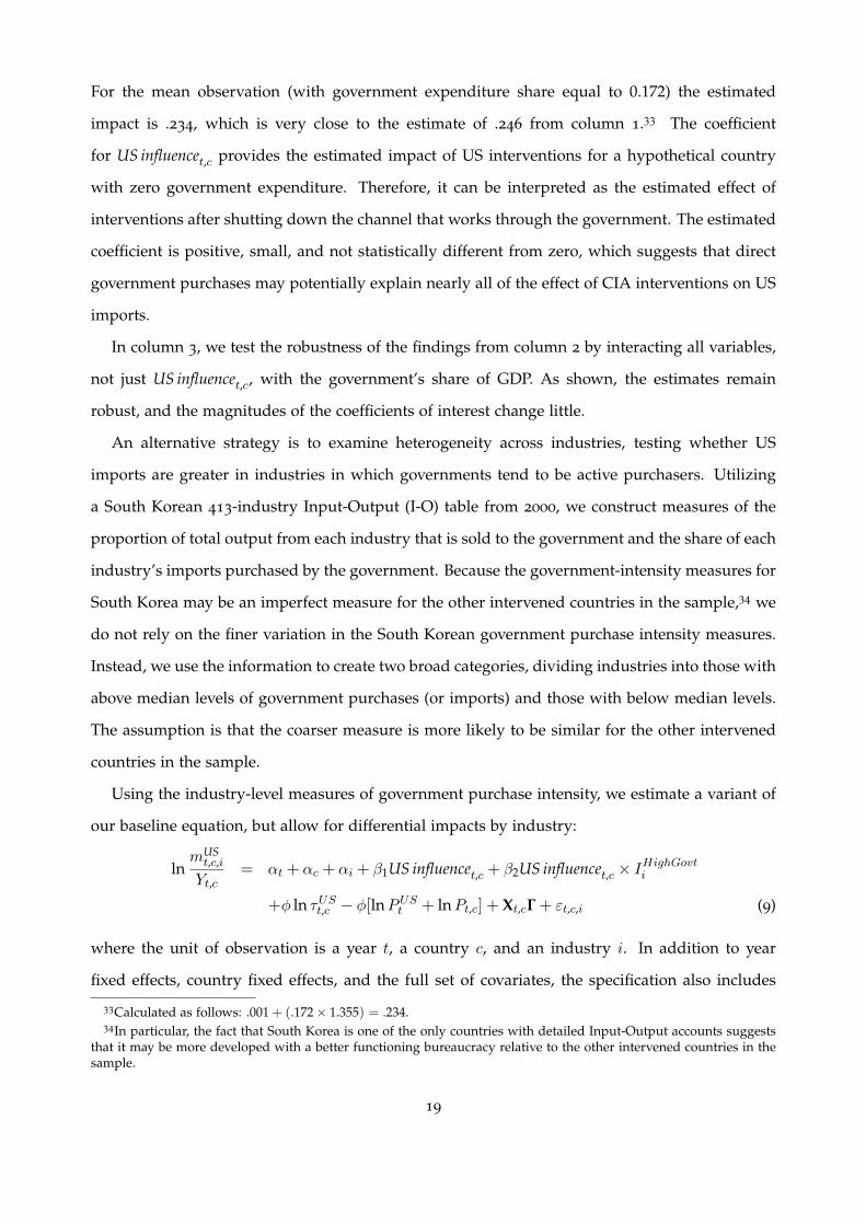
For the mean observation (with government expenditure share equal to 0.172) the estimated

impact is .234, which is very close to the estimate of .246 from column 1.33 The coefficient

for US influencet,c provides the estimated impact of US interventions for a hypothetical country

with zero government expenditure. Therefore, it can be interpreted as the estimated effect of

interventions after shutting down the channel that works through the government. The estimated

coefficient is positive, small, and not statistically different from zero, which suggests that direct

government purchases may potentially explain nearly all of the effect of CIA interventions on US

imports.

In column 3, we test the robustness of the findings from column 2 by interacting all variables,

not just US influencet,c, with the government’s share of GDP. As shown, the estimates remain

robust, and the magnitudes of the coefficients of interest change little.

An alternative strategy is to examine heterogeneity across industries, testing whether US

imports are greater in industries in which governments tend to be active purchasers. Utilizing

a South Korean 413-industry Input-Output (I-O) table from 2000, we construct measures of the

proportion of total output from each industry that is sold to the government and the share of each

industry’s imports purchased by the government. Because the government-intensity measures for

South Korea may be an imperfect measure for the other intervened countries in the sample,34 we

do not rely on the finer variation in the South Korean government purchase intensity measures.

Instead, we use the information to create two broad categories, dividing industries into those with

above median levels of government purchases (or imports) and those with below median levels.

The assumption is that the coarser measure is more likely to be similar for the other intervened

countries in the sample.

Using the industry-level measures of government purchase intensity, we estimate a variant of

our baseline equation, but allow for differential impacts by industry:

lnmUSt,c,i

Yt,c= αt + αc + αi + β1US influencet,c + β2US influencet,c × I

HighGovti

+φ ln τUSt,c − φ[lnPUSt + lnPt,c] + Xt,cΓ + εt,c,i (9)

where the unit of observation is a year t, a country c, and an industry i. In addition to year

fixed effects, country fixed effects, and the full set of covariates, the specification also includes

33Calculated as follows: .001 + (.172× 1.355) = .234.34In particular, the fact that South Korea is one of the only countries with detailed Input-Output accounts suggests

that it may be more developed with a better functioning bureaucracy relative to the other intervened countries in thesample.

19

industry fixed effects. As well, the dependent variable is the natural log of imports from the US

into country c in year t in industry i (normalized by total GDP). Unlike the aggregate-level COW

trade data, the industry level data, which are from the United Nations’ Comtrade Database, only

begin in 1962. Therefore the sample only includes years between 1962 and 1989.

Estimates of equation (9), reported in columns 4 and 5 of table 2, show that the impact of CIA

interventions is greater in industries for which governments are active consumers and importers.

The impact in government-intensive industries is 72% greater in column 4, and by 54% greater

in column 5; both differences are statistically significant. Therefore, evidence from industry

heterogeneity also suggests that government purchases are an important part of the explanation

for the increase in US imports.

We also examine whether there is evidence that US influence was used to liberalize trade or

foreign direct investment (FDI) policies, which in turn may have led to increased imports from the

US. We find no evidence for either mechanism. Using data from the Bureau of Economic Analysis

we examine whether interventions were followed by increases in US FDI in the intervened

country. We find no evidence of a positive relationship between interventions and FDI. As well,

controlling for US FDI has no impact on the relationship between CIA interventions and imports

from the US (see appendix table A8, columns 1–4).

We test for the tariff mechanism using information from the International Customs Journal, an

International Customs Tariff Bureau publication, that reporting countries’ tariff schedules on a

continuous basis. When a country significantly changes its tariff structure, a new ‘volume’ is

published for the country. If minor changes to the tariff structure are made, then a ‘supplement’

to the most recent volume is published. Therefore, we use the publication of a new volume as an

indication that there was restructuring of the country’s tariffs. We find that CIA interventions had

no impact on the probability of a change in the tariffs structure. We also find that US interventions

did not have a greater impact on US imports after a revision to the intervened-country’s tariff

schedule (see appendix table A8, columns 5–7).35

35In practice, this is implemented by constructing a variable that equals one for interventions that follow a changein the tariff structure during an intervention episode.

20

6. Testing Alternative Explanations

A. Trade Integration Explanation

We now turn to potential alternative explanations for the relationship between CIA interven-

tions and increased US imports. A plausible alternative explanation is that CIA interventions

resulted in increased openness between the US and the intervened country, and this increased

the country’s imports from the US (but not exports to the US). To test for this possibility, we

move to the industry level and examine which industries experienced the greatest surge in US

imports following an intervention. If the increase in imports arose because of a decrease in trading

frictions, then the increase in shipments from the US should have been in industries in which the

US had a comparative advantage. With an increase in openness, countries increasingly export

the goods that they have a relative cost advantage in producing and import the goods they have

a relative disadvantage in producing. This logic of comparative advantage is central to standard

models of international trade ranging from the textbook Ricardian or Heckscher-Ohlin models of

trade to more recent models of comparative advantage with firm heterogeneity (e.g., Andrew B.

Bernard, Stephen J. Redding and Peter K. Schott, 2007).36

Testing the trade integration explanation requires a measure of US competitiveness across in-

dustries and time periods. For this we use Bella Balassa’s (1965) measure of revealed comparative

advantage (RCA). The measure, which captures the degree of specialization of a country in a

particular industry, is given by:

RCAt,c,i =xt,c,i

∑c xt,c,i

/ ∑i xt,c,i

∑i ∑c xt,c,i

where xt,c,i denotes the aggregate exports of country c in a 2, 3 or 4-digit Standard International

Trade Classification (SITC) industry i in year t. The RCA measure is a ratio of two ratios. The

first ratio, the numerator, is country c’s share of world exports in industry i. The second ratio,

the denominator, is country c’s share of world exports in all industries. Thus, RCA compares a

country’s share of global exports in industry i to its share across all industries. If the ratio is

36The only model that we are aware of for which a slightly weaker version of this holds is Rudiger Dornbusch,Stanley Fischer and Paul A. Samuelson (1977). In this setting, trade costs generate a range of goods that are non-traded(i.e., produced by both countries). Greater integration decreases this range and each country begins to export thepreviously non-traded goods for which they have a comparative advantage. Although the new exports are comparativeadvantage goods, they are not the goods for which the countries have the greatest comparative advantage, since thesegoods were already being exported. However, within the model, a decrease in trade costs still increases the exports ofgoods for which the country has a comparative advantage.

21

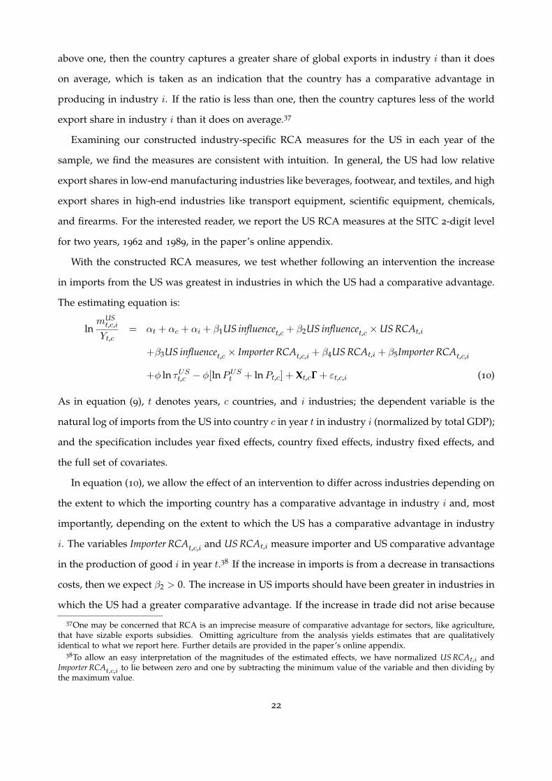
above one, then the country captures a greater share of global exports in industry i than it does

on average, which is taken as an indication that the country has a comparative advantage in

producing in industry i. If the ratio is less than one, then the country captures less of the world

export share in industry i than it does on average.37

Examining our constructed industry-specific RCA measures for the US in each year of the

sample, we find the measures are consistent with intuition. In general, the US had low relative

export shares in low-end manufacturing industries like beverages, footwear, and textiles, and high

export shares in high-end industries like transport equipment, scientific equipment, chemicals,

and firearms. For the interested reader, we report the US RCA measures at the SITC 2-digit level

for two years, 1962 and 1989, in the paper’s online appendix.

With the constructed RCA measures, we test whether following an intervention the increase

in imports from the US was greatest in industries in which the US had a comparative advantage.

The estimating equation is:

lnmUSt,c,i

Yt,c= αt + αc + αi + β1US influencet,c + β2US influencet,c ×US RCAt,i

+β3US influencet,c × Importer RCAt,c,i + β4US RCAt,i + β5Importer RCAt,c,i

+φ ln τUSt,c − φ[lnPUSt + lnPt,c] + Xt,cΓ + εt,c,i (10)

As in equation (9), t denotes years, c countries, and i industries; the dependent variable is the

natural log of imports from the US into country c in year t in industry i (normalized by total GDP);

and the specification includes year fixed effects, country fixed effects, industry fixed effects, and

the full set of covariates.

In equation (10), we allow the effect of an intervention to differ across industries depending on

the extent to which the importing country has a comparative advantage in industry i and, most

importantly, depending on the extent to which the US has a comparative advantage in industry

i. The variables Importer RCAt,c,i and US RCAt,i measure importer and US comparative advantage

in the production of good i in year t.38 If the increase in imports is from a decrease in transactions

costs, then we expect β2 > 0. The increase in US imports should have been greater in industries in

which the US had a greater comparative advantage. If the increase in trade did not arise because

37One may be concerned that RCA is an imprecise measure of comparative advantage for sectors, like agriculture,that have sizable exports subsidies. Omitting agriculture from the analysis yields estimates that are qualitativelyidentical to what we report here. Further details are provided in the paper’s online appendix.

38To allow an easy interpretation of the magnitudes of the estimated effects, we have normalized US RCAt,i andImporter RCAt,c,i to lie between zero and one by subtracting the minimum value of the variable and then dividing bythe maximum value.

22

Table 3: Testing the trade costs explanation using revealed comparative advantage.

2-digit industries 3-digit industries 4-digit industries 2-digit industries 3-digit industries 4-digit industries(1) (2) (3) (4) (5) (6)

US influence 0.524*** 0.447*** 0.391*** 0.532*** 0.465*** 0.390***(0.107) (0.093) (0.088) (0.107) (0.091) (0.085)

US influence × US RCA -1.202** -1.496** -1.511** -1.601** -1.426*** -1.290***(0.490) (0.632) (0.590) (0.622) (0.520) (0.438)

US RCA 2.279*** 4.804*** 4.103*** 3.004*** 3.494*** 2.383***(0.259) (0.213) (0.182) (0.313) (0.263) (0.321)

Observations 131,895 330,358 553,842 131,895 330,358 553,842Notes: The unit of observation is a country c in year t in a 2, 3 or 4-digit SITC industry i, where t ranges from 1962 to 1989. The dependent variable isthe natural log of imports form the US normalized by total GDP. All regressions include year fixed effects, country fixed effects, industry fixed effects,Baier and Bergstrand multilateral resistance terms, a Soviet intervention control, importer RCA, importer RCA interacted with US influence, ln percapita income, an indicator for leader turnover, current leader tenure, a democracy indicator, as well as Baier and Bergstrand (2009) controls for tradecosts and multilateral resistance terms. These are a function of the natural log of bilateral distance, an indicator variable for a common language, anindicator variable for a shared border, an indicator for both trading partners being GATT participants and an indicator for the trading partners beingpart of a regional trade agreement. Coefficients are reported with standard errors clustered at the country-year level in brackets. ***, **, and *indicate significance at the 1, 5 and 10% levels.

Dependent variable: ln normalized imports from the US

World market RCA Developing country market RCA

of comparative advantage, then we no longer expect β2 > 0. Instead, it is likely that the US

pushed to sell less competitive products that firms would have difficulty selling otherwise. If this

was the case then we expect β2 ≤ 0. Therefore, the sign of β2 provides a test of the integration

and influence explanations.

Estimates of equation (10) are reported in columns 1–3 of table 3. We report standard

errors clustered at the country-year level.39 In all specifications, the estimated coefficients for

US influencet,c ×US RCAt,c are negative and statistically significant, indicating that interventions

increased imports more in industries in which the US had a comparative disadvantage, not

comparative advantage. This finding is in contrast to what is expected if the increase in trade

were from increased integration with the US.40

A potential criticism of the RCA measure is that it does not distinguish between a country’s

exports to developed countries (DCs) and its exports to less developed countries (LDCs). The

39Clustering produces standard errors that are larger in magnitude than Newey-West standard errors. Therefore, tobe as conservative as possible, we report the clustered standard errors.

40The total effect of US influencet,c on imports from the US is given by β1 +β2 US RCAt,i+β3 Importer RCAt,c,i. Exam-ining this, we find that for nearly all observations (countries, years, and industries), the total effect of US influencet,c isgreater than or equal to zero. This is also confirmed when we estimate equation (7) industry-by-industry.41 Therefore,CIA interventions had a non-negative effect on the purchase of US products in nearly every industry, and the effectswere greatest in industries in which the US was globally least competitive.

23

two groups of countries may represent different segmented markets. Since the market size of

LDCs is much smaller than of DCs, when the US serves the LDC market, its share of total world

exports may be low, and therefore its measure of RCA may also be low. If interventions decreased

bilateral trade costs between the US and the intervened LDCs, then this may have caused the US

to specialize more in products that serve the LDC market and, as a result, imports from the US

increased most in industries with low measures of RCA.

According to this explanation, the test fails because we are incorrectly measuring RCA. Rather

than measuring RCA using exports to the whole world, we should measure RCA using exports

to LDCs only. We check for this possibility by constructing an alternative measure of RCA that

is calculated using only the share of exports to LDCs, rather than the share of exports globally.42

Estimates using the alternative RCA measure are reported in columns 4–6 of table 3. As shown,

the results are nearly identical using the alternative RCA measure.

Overall, the results provide evidence against the hypothesis that the increase in US imports

following an intervention was the result of increased integration with the US.

B. Political Ideology Explanation

In light of existing evidence that countries with more similar political ideologies trade more (e.g.,

William J. Dixon and Bruce E. Moon, 1993), it is possible that the increase in imports from the US

can be explained by a change in the ideology of the intervened country following an intervention.

According to this explanation, the increase in US imports arose not because of US influence, but

because the new regime has an ideology that is more aligned with Western countries, including

the US.

Testing this hypothesis requires that we examine whether imports from countries with an

ideology similar to the US also increased following CIA interventions. Our current estimating

equations, because they only examine a country’s imports from the US, cannot be used for this

purpose. Therefore, we estimate a regression that examines each country’s imports from all

exporters, not just the US. The estimating equation, derived from equation (2) in section 3, is

42We define the LDC market to be countries other than Australia, Austria, Belgium, Canada, Switzerland, East andWest Germany, Denmark, Great Britain, Ireland, Italy, France, Finland, Japan, Luxembourg, Norway, Netherlands,New Zealand, Portugal, Spain, and Sweden.

24

given by:

lnmt,c,e

Yt,cYt,e= αt + αc,e + β1US influencet,c + β2US influencet,c × I

USe

+φ ln τt,c,e − φ[lnPt,c + lnPt,e] + Xt,cΓ + Xt,eΩ (11)

where t indexes years, c indexes importers, and e indexes exporters. The dependent variable

is the natural log of imports into country c from exporting country e in year t divided by the

product of the total GDP of countries c and e. Equation (11) includes time period fixed effects αt,

and country-pair fixed effects αc,e, as well as the same vector of importer covariates as in equation

(7), Xt,c. Also included are the same covariates, but measured for exporters, Xt,e.

As in equation (7), our variable of interest is US influencet,c, which equals one if the importing

country c experienced a CIA intervention in year t. Because we now include all country-pairs in

the sample, we allow the effect of interventions on imports to differ depending on whether the

exporter is American or not. In practice, this is done by also including US influencet,c × IUSe in the

estimating equation, where IUSe is an indicator variable that equals one if the exporter is the US.

The coefficient, β2, provides a test of whether the impact of CIA interventions on imports from

the US (β1 + β2) are statistically different than the impact on imports from other countries (β1).

The estimate of equation (11), reported in column 1 of table 4, yields results that are qualita-

tively identical to the baseline findings. According to the estimates of β1 and β2, interventions

decreased imports from non-US countries by 4.6% and increased imports from the US by 26.8%,

which is very similar to the estimate of 30.3% from equation (7) reported in column 3 of table

1. The estimated negative impact on non-US exporters is also consistent with the finding from

table 1 that the increase in US imports arose through trade diversion and not trade creation. The

magnitudes of β1 and β2 suggest that the increase in imports from the US is roughly offset by the

decrease in imports from other.43

We next test whether the differential impact of CIA interventions on imports from the US is

robust to controlling for the ideology of exporters. We use US ideology as a reference point and

construct a measure of similarity to the US using voting data from the UN General Assembly.

Define dt,c to be the sum of the vote distance between country c and the US for all votes in year t,

where a vote in opposition to the US is given a distance of one, and a vote with the US is given a

43To see this, first note that for the average observation, the share of total imports that are from the US is 18.9%. Ifwe let mo denote a country’s initial level of total imports, then the predicted intervention-induced increase in importsfrom the increase in US trade is given by .268× .189×mo = .051mo. The decrease in imports from non-US exportersis given by .046× .811×mo = .037mo.

25

distance of zero.44 Also define dmaxt to be the maximum sum of vote distances possible in year t.

We then construct the following measure of country c’s voting similarity with the US in year t:

V USt,c ≡ 1− dt,c

dmaxt

The measure ranges from 0 to 1, and is increasing in the vote similarity of the country with the

US.45

With V USt,c we can test whether following US interventions, imports from countries that were

ideologically similar to the US also increased, and whether the differential impact of CIA inter-

ventions on imports from the US remains robust to controlling for ideology. In practice, this

is done by altering equation (11) to allow the impact of CIA interventions on imports to differ

systematically depending on the political ideology of the exporter:

lnmt,c,e

Yt,cYt,m= αt + αc,e + β1US influencet,c + β2US influencet,c × I

USe + β3US influencet,c × V

USt,e

+β4VUSt,e + φ ln τt,c,e − φ[Pt,c + Pt,e] + Xt,cΓ + Xt,eΩ + εt,c,e (12)

The added interaction term, US influencet,c × V USt,e , controls for the possibility that exports from

countries that were ideologically similar to the US also increased following CIA interventions. If

β2, the coefficient for US influencet,c × IUSe , becomes insignificant with the addition of this control,

this is evidence for the political alignment explanation. We are also interested in the sign of β3,

the coefficient for US influencet,c × V USt,e . If the ideology explanation is correct then we expect the

coefficient to be positive.

Estimation results are reported in column 2 of table 4. The estimate of β2 remains robust to the

inclusion of the new interaction term. The coefficient remains positive and significant, suggesting

the existence of a greater impact of CIA intervention on imports from the US even after allowing

for heterogeneity based on exporters’ political ideology. The bottom panel of the table reports the

estimated impact of CIA interventions on imports from the US and on imports from a country

with a value of V USt,e equal to the sample average. The calculated impact for the US is very similar

44See Erik Gartzke (2006) for details. The measure we use ignores abstentions. An alternative is to code a valueof two for votes against the US, a value of one for abstentions, and zero for votes with the US. Using this alternativecoding yields qualitatively identical results to what we report here.

45One concern is that voting similarity may not accurately reflect similarity in political ideology. We check thispossibility by examining the correlation between a country’s voting alignment with the US and a measure of left,center or right political alignment from Philip Keefer (2005). The political alignment data are only available from 1975.However, coding left, center and right alignments as 1, 2 and 3, respectively, we find a strong positive correlationbetween the two measures. Regressing US vote similarity on political alignment yields a standardized beta coefficientof 0.29 and a t-statistic of 10.55.

26

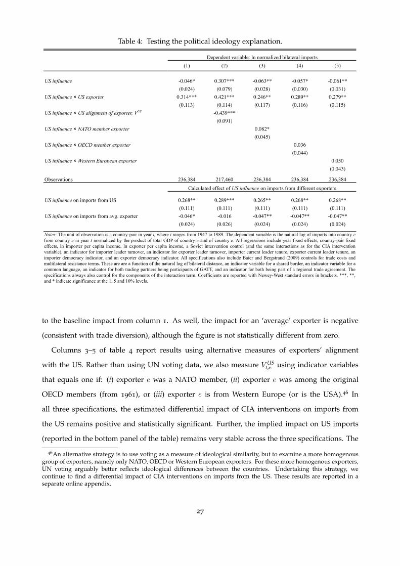
Table 4: Testing the political ideology explanation.

(1) (2) (3) (4) (5)

US influence -0.046* 0.307*** -0.063** -0.057* -0.061**(0.024) (0.079) (0.028) (0.030) (0.031)

US influence × US exporter 0.314*** 0.421*** 0.246** 0.289** 0.279**(0.113) (0.114) (0.117) (0.116) (0.115)

US influence × US alignment of exporter, VUS -0.439***(0.091)

US influence × NATO member exporter 0.082*(0.045)

US influence × OECD member exporter 0.036(0.044)

US influence × Western European exporter 0.050(0.043)

Observations 236,384 217,460 236,384 236,384 236,384

US influence on imports from US 0.268** 0.289*** 0.265** 0.268** 0.268**(0.111) (0.111) (0.111) (0.111) (0.111)

US influence on imports from avg. exporter -0.046* -0.016 -0.047** -0.047** -0.047**(0.024) (0.026) (0.024) (0.024) (0.024)

Notes: The unit of observation is a country-pair in year t, where t ranges from 1947 to 1989. The dependent variable is the natural log of imports into country c from country e in year t normalized by the product of total GDP of country c and of country e. All regressions include year fixed effects, country-pair fixedeffects, ln importer per capita income, ln exporter per capita income, a Soviet intervention control (and the same interactions as for the CIA interventionvariable), an indicator for importer leader turnover, an indicator for exporter leader turnover, importer current leader tenure, exporter current leader tenure, animporter democracy indicator, and an exporter democracy indicator. All specifications also include Baier and Bergstrand (2009) controls for trade costs andmultilateral resistance terms. These are are a function of the natural log of bilateral distance, an indicator variable for a shared border, an indicator variable for acommon language, an indicator for both trading partners being participants of GATT, and an indicator for both being part of a regional trade agreement. Thespecifications always also control for the components of the interaction term. Coefficients are reported with Newey-West standard errors in brackets. ***, **,and * indicate significance at the 1, 5 and 10% levels.

Dependent variable: ln normalized bilateral imports

Calculated effect of US influence on imports from different exporters

to the baseline impact from column 1. As well, the impact for an ‘average’ exporter is negative

(consistent with trade diversion), although the figure is not statistically different from zero.

Columns 3–5 of table 4 report results using alternative measures of exporters’ alignment

with the US. Rather than using UN voting data, we also measure V USt,e using indicator variables

that equals one if: (i) exporter e was a NATO member, (ii) exporter e was among the original

OECD members (from 1961), or (iii) exporter e is from Western Europe (or is the USA).46 In

all three specifications, the estimated differential impact of CIA interventions on imports from

the US remains positive and statistically significant. Further, the implied impact on US imports

(reported in the bottom panel of the table) remains very stable across the three specifications. The

46An alternative strategy is to use voting as a measure of ideological similarity, but to examine a more homogenousgroup of exporters, namely only NATO, OECD or Western European exporters. For these more homogenous exporters,UN voting arguably better reflects ideological differences between the countries. Undertaking this strategy, wecontinue to find a differential impact of CIA interventions on imports from the US. These results are reported in aseparate online appendix.

27

implied impact of CIA interventions on the average non-US exporter is negative and statistically

significant in each specification. Further the magnitude is very similar to the baseline magnitude

reported in column 1 of the table. As well, we find that as in column 2, there is no statistically

significant differential impact of CIA interventions based on a country’s political alignment with

the US. The one exception is for NATO membership, where we estimate a positive and significant

differential impact. However, according to the magnitudes of the coefficient estimates, the impact

of CIA interventions on imports from NATO members is still zero (with a coefficient of .019 (i.e.,

−0.063 + 0.082) and standard error of .037).

C. US Loans and Grants Explanation

If interventions led to an increase in foreign aid from the US, particularly tied or conditional aid,

then this could explain the increase in US imports.47 To test for this possibility, we examine the

value of US economic aid (which includes grants and concessional loans) and military aid (which

includes grants, concessional loans, and training) received by each country, and test whether CIA

interventions led to an increase in US foreign aid, and whether the changes in aid are able to

account for the observed increase in US imports.48

In columns 1 and 2 of table 5, we report estimates of our baseline estimating equation (7) with

either military aid or economic aid as the dependent variable.49 The results show that both forms

of aid increased following CIA interventions. In column 3, we examine loans given by the US

Export-Import Bank (Ex-Im Bank), an institution with a mandate to provide loans to foreign firms

that want but are having trouble obtaining financing from private lenders. The estimate from

column 3 shows that CIA interventions also led to an increase in Ex-Im Bank loans, although the

magnitude of the impact and statistical significance is lower than for either type of foreign aid.

Columns 4–7 of table 5 report estimates that test whether the increase in aid and loans are

able to account for the increase in US imports following an intervention. We do this by estimating

equation (7) while controlling for military aid, economic aid, and Ex-Im Bank loans. The variables

47The fact that US imports increased most in low US RCA industries suggests that if this explanation is correct, thenthe provision of grants and loans were used to promote US sales in industries in which US firms were less competitive.This would also be an interesting and important finding.

48The data are from the US Agency for International Development’s (USAID) US Overseas Loans and Grants, Obliga-tions and Loan Authorizations.

49The aid variables are measured as the natural log of one plus their value. The specifications reported do notinclude the controls for multilateral resistance terms. The results are qualitatively identical if these terms are included.

28

Table 5: The role of US loans and grants.

Military aidEconomic

aidEx-Im Bank

loans(1) (2) (3) (4) (5) (6) (7) (8)

US influence 0.802*** 0.807*** 0.199* 0.303*** 0.280*** 0.261** 0.292*** 0.254**(0.210) (0.241) (0.121) (0.110) (0.107) (0.101) (0.107) (0.099)

ln (1+US military aid) 0.033 -0.011(0.031) (0.028)

ln (1+US economic aid) 0.059** 0.064***(0.026) (0.023)

ln ( 1+Ex-Im Bank loans) 0.049*** 0.050***(0.014) (0.014)

Observations 4,149 4,149 4,149 4,149 4,149 4,149 4,149 4,149

Notes : The unit of observation is a country c in year t, where t ranges from 1947 to 1989. In columns 1-3, the dependent variables are thenatural log of the measure of aid that is reported in the column heading. In columns 4-8, the dependent variable is the natural log of importsfrom the US divided by total GDP. All regressions include year fixed effects, country fixed effects, a Soviet intervention control, ln per capitaincome, an indicator for leader turnover, current leader tenure, and a democracy indicator. Columns 4-8 also include Baier and Bergstrand(2009) controls for trade costs and multilateral resistance terms. These are a function of the natural log of bilateral distance, an indicatorvariable for a common language, an indicator variable for a shared border, an indicator for both trading partners being GATT participants andan indicator for the trading partners being part of a regional trade agreement. Coefficients are reported with Newey-West standard errors inbrackets. ***, **, and * indicate significance at the 1, 5 and 10% levels.

Dependent variable:

ln normalized imports from the US

enter one at a time in columns 4–6 and simultaneously in column 7. We find that economic

aid enters with positive and significant coefficients, while military aid enters with insignificant

coefficients that are very close to zero. This suggests that part of US economic aid was used to

import US products, which is unsurprising since US economic aid is often tied to purchases from

US producers. The insignificant coefficient for military aid is also unsurprising, since much of

military aid is spent on goods exported overseas to support US troops and other personnel, and

these goods are not included in the IMF’s DOT statistics (International Monetary Fund, 1993).

The coefficient for Ex-Im Bank loans is also positive, as expected.

Controlling for the grants and loans variables we observe a modest decline in the estimated

coefficients for US influencet,c. The coefficient magnitudes are reduced by at most 16% (in column

7). This suggests that although increases in US loans and grants are able to explain some of the

effect of interventions on imports from the US, it is a modest proportion of the total. This is

consistent with the fact that foreign aid flows are not large enough to account for the observed

29

increase in imports from the US.50

These results come with the important caveat that the aid measures used in the analysis only

include official aid flows and do not include covert aid from the CIA. Therefore, we are unable to

rule out the possibility that the impact of CIA interventions are explained by covert aid.

7. Conclusions

We have provided evidence that covert CIA interventions increased the influence of the US over

foreign governments, and that this was used to increase US exports to the intervened countries.

Consistent with the influence mechanism, the increase was greatest in industries in which the US

had a comparative disadvantage. Our analysis was able to rule out alternative explanations for

the increase in imports from the US, including decreased trade costs, changing political ideology

and increased US loans and grants.

Our findings contribute to several literatures. First, they complement the existing evidence

on the importance of political economy determinants of trade flows by showing that CIA inter-

ventions also affect the pattern of trade.51 As well, by isolating the role of political influence,

our findings provide support for existing evidence that influence and power play an important

role in international trade.52 Finally, our findings also add to existing studies that examine, both

qualitatively and quantitatively, the history of the CIA using recently declassified documents.53

There are a number of natural directions for future research. The first is a more fine-grained

examination of the mechanisms underlying our results. Although the macro-level evidence we

have presented indicate that government procurement contracts play an important role, we still

require a deeper understanding of the precise mechanisms. Most likely, this requires micro-

level data that captures the means by which government contracts are assigned to suppliers

from the US, and the precise lobbying/bidding process by which low comparative advantage

manufacturers are able to gain a disproportionate share of these contracts. The second is to

50The ratio of US total aid to US imports is 0.15 for the median observation in the sample. Therefore, even if anintervention-induced increase in US aid was transformed one-for-one into imports (which in reality is far from true),CIA interventions would need to increase aid by 202% to increase imports by the observed 30.3% (202%× 0.15 =30.3%). The estimated effects of interventions on US aid found in columns 1–3 of table 5 are much lower than this,ranging instead from between 20 and 81%.

51See for example Verdier (1998), Mansfield, Milner and Rosendorff (2000), Russett and Oneal (2001), Mansfield,Milner and Rosendorff (2002), Frye and Mansfield (2003), Kono (2006) and Mansfield, Milner and Pevehouse (2008).

52See Yeats (1990), Joanne Gowa and Edward D. Mansfield (1993), Mansfield, Milner and Rosendorff (2002),Kuziemko and Werker (2006), Dreher and Jensen (2007), and Kilby (2009).

53See for example Weiner (2007) and Dube, Kaplan and Naidu (2011).

30

examine additional consequences of CIA interventions. We have examined the effects of a specific

type of CIA intervention on one dimension of international trade. However, interventions may

have had a host of additional impacts, both at macro and micro levels. For instance, the financial

consequences of CIA interventions remain largely unexplored and may constitute a promising

area of future research.

References

Aidt, Toke S., and Martin Gassebner. 2010. “Do Autocratic States Trade Less?” World BankEconomic Review, 24(1): 38–76.

Alvarez, Mike, José Antonio Cheibub, Fernando Limongi, and Adam Przeworski. 1996. “Clas-sifying Political Regimes.” Studies in Comparative International Development, 31(2): 3–36.

Anderson, James, and Eric van Wincoop. 2003. “Gravity with Gravitas: A Solution to the BorderPuzzle.” American Economic Review, 93(1): 170–192.

Andrew, Christopher, and Vasili Mitrokhin. 2000. The Sword and the Shield: The Mitrokhin Archiveand the Secret History of the KGB. New York:Basic Books.

Andrew, Christopher, and Vasili Mitrokhin. 2005. The World Was Going Our Way. New York:BasicBooks.

Antràs, Pol, and Gerard Padró-i-Miquel. 2011. “Foreign Influence and Welfare.” Journal of Inter-national Economics, 84(2): 135–148.

Audet, Denis. 2002. “Government Procurement: A Synthesis Report.” OECD Journal of Budgeting,2(3): 149–194.

Baier, Scott L., and Jeffrey H. Bergstrand. 2009. “Bonus Vetus OLS: A Simple Method for Approx-imating International Trade-Cost Effects using the Gravity Equation.” Journal of InternationalEconomics, 77: 77–85.

Balassa, Bella. 1965. “Trade Liberalization and ‘Revealed’ Comparative Advantage.” The Manch-ester School of Economics and Social Studies, 32(2): 99–123.

Baldwin, Robert E. 1970. Nontariff Distortions of International Trade. Washington D.C.:The Brook-ings Institution.

Barbieri, Katherine, Omar M.G. Keshk, and Brian M. Pollins. 2008. “Correlates of War ProjectTrade Data Set Codebook, Version 2.0.” Mimeo, June 17, 2008.

Barbieri, Katherine, Omar M.G. Keshk, and Brian M. Pollins. 2009. “Trading Data: Evaluatingour Assumptions and Coding Rules.” Conflict Management and Peace Science, 26(5): 471–491.

Berger, Daniel, Alejandro Corvalan, William Easterly, and Shanker Satyanath. 2010. “Super-power Interventions and their Consequences for Democracy: An Empirical Inquiry.” Mimeo,New York University.

Bernard, Andrew B., Stephen J. Redding, and Peter K. Schott. 2007. “Comparative Advantageand Heterogeneous Firms.” Review of Economic Studies, 74(1): 31–66.

31

Bertrand, Marianne, Esther Duflo, and Sendhil Mullainathan. 2004. “How Much Should WeTrust Differences-in-Differences Estimates?” Quarterly Journal of Economics, 119(1): 249–275.

Blum, William. 2004. Killing Hope: U.S. Military and C.I.A. Interventions since World War II. Monroe,ME:Common Courage Press.

Chaney, Thomas. 2008. “Distorted Gravity: Heterogeneous Firms, Market Structure and theGeography of International Trade.” American Economic Review, 98(4): 1707–1721.

Cheibub, José Antonio, Jennifer Gandhi, and James Raymond Vreeland. 2010. “Democracy andDictatorship Revisited.” Public Choice, 143: 67–101.

Cingano, Federico, and Paolo Pinotti. 2010. “Politicians at Work: The Private Returns and SocialCosts of Political Connections.” Mimeo, Bank of Italy.

Dixon, William J., and Bruce E. Moon. 1993. “Political Similarity and American Foreign TradePatterns.” Political Research Quarterly, 46(1): 5–25.

Dornbusch, Rudiger, Stanley Fischer, and Paul A. Samuelson. 1977. “Comparative Advantage,Trade and Payments in a Ricardian Model with a Continuum of Goods.” American EconomicReview, 67(5): 823–839.

Dreher, Axel, and Nathan M. Jensen. 2007. “Independent Actor or Agent? An Empirical Analysisof the Impact of U.S. Interests on International Monetary Fund Conditions.” Journal of Law andEconomics, 50(1): 105–124.

Dube, Arindrajit, Ethan Kaplan, and Suresh Naidu. 2011. “Coups, Corporations, and ClassifiedInformation.” Quarterly Journal of Economics, 126(3): 1375–1409.

Eaton, Jonathan, and Samuel Kortum. 2002. “Technology, Geography and Trade.” Econometrica,70(5): 1741–1779.

Erikson, Robert S., Pablo M. Pinto, and Kelly T. Rader. 2009. ““Dirty Pool” Revisited: WhenLess is More.” Mimeo, Columbia University.

Findlay, Ronald, and Kevin H. O’Rourke. 2007. Power and Plenty: Trade, War, and the WorldEconomy in the Second Millennium. Princeton:Princeton University Press.

Frye, Timothy, and Edward D. Mansfield. 2003. “Fragmenting Protection: The Political Economyof Trade Policy in the Post-Communist World.” British Journal of Political Science, 33(4): 635–657.

Gartzke, Erik. 2006. “The Affinity of Nations Index, 1946–2002.” Mimeo, Columbia University.

Goldman, Eitan, Jorg Rocholl, and Jongil So. 2008. “Political Connections and the Allocation ofProcurement Contracts.” Mimeo, Indiana University.

Gowa, Joanne, and Edward D. Mansfield. 1993. “Power, Politics and International Trade.”American Political Science Review, 87(2): 408–420.

Head, Keith, Thierry Mayer, and John Ries. 2010. “The Erosion of Colonial Trade Linkages afterIndependence.” Journal of International Economics, 81(1): 1–14.

Hirschman, Albert O. 1945. National Power and the Structure of Foreign Trade. Berkeley:Universityof California Press.

32

Hufbauer, Gary Clyde, Jeffrey J. Schott, Kimberly Ann Elliott, and Barbara Oegg. 2009. Eco-nomic Sanctions Reconsidered, 3rd Edition. Washington, D.C.:Peterson Institute for InternationalEconomics.

International Monetary Fund. 1993. A Guide to Direction of Trade Statistics. Washington, D.C.:IMFStatistics Department.

Johnson, Loch K. 1989. “Covert Action and Accountability: Decision-Making for America’s SecretForeign Policy.” International Studies Quarterly, 33(1): 81–109.

Johnson, Loch K. 1992. “On Drawing a Bright Line for Covert Operations.” American Journal ofInternational Law, 86(2): 284–309.

Jones, Benjamin, and Benjamin Olken. 2005. “Do Leaders Matter? National Leadership andGrowth Since World War II.” Quarterly Journal of Economics, 120(3): 835–864.

Jones, Benjamin, and Benjamin Olken. 2009. “Hit or Miss? The Effect of Assassinations onInstitutions and War.” American Economic Journal: Macroeconomics, 1(2): 55–87.

Keefer, Philip. 2005. “Database of Political Institutions: Changes and Variable Definitions.”Mimeo, Development Research Group, World Bank.

Kilby, Christopher. 2009. “The Political Economy of Conditionality: An Empirical Analysis ofWorld Bank Loan Disbursements.” Journal of Development Economics, 89(1): 51–61.

Kono, Daniel Y. 2006. “Optimal Obfuscation: Democracy and Trade Policy Transparency.” Amer-ican Political Science Review, 100(3): 369–384.

Kuziemko, Ilyana, and Eric Werker. 2006. “How Much is a Seat on the Security Council Worth?Foreign Aid and Bribery at the United Nations.” Journal of Political Economy, 114(5): 905–930.

Leary, William M. 1984. The Central Intelligence Agency: History and Documents. Tuscaloosa,AL:University of Alabama Press.

Lowinger, Thomas C. 1976. “Discrimination in Government Procurement of Foreign Goods inthe U.S. and Western Europe.” Southern Economic Journal, 42(3): 451–460.

Mansfield, Edward D., Helen V. Milner, and B. Peter Rosendorff. 2000. “Free to Trade: Democ-racies, Autocracies, and International Trade.” American Political Science Review, 94(2): 305–321.

Mansfield, Edward D., Helen V. Milner, and B. Peter Rosendorff. 2002. “Why DemocraciesCooperate More: Electoral Control and International Trade Agreements.” International Organi-zation, 56(3): 477–513.

Mansfield, Edward D., Helen V. Milner, and Jon C. Pevehouse. 2008. “Democracy, Veto Playersand the Depth of Regional Integration.” World Economy, 31(1): 67–96.

Maoz, Zeev. 2005. “Dyadic MID Dataset (version 2.0).” UC Davis.

Russett, Bruce, and John R. Oneal. 2001. Triangulating Peace: Democracy, Interdependence, andInternational Organizations. New York:Norton.

Santos Silva, J.M.C., and Silvana Tenreyro. 2006. “The Log of Gravity.” Review of Economics andStatistics, 88(4): 641–658.

Sylvan, David, and Stephen Majeski. 2009. U.S. Foreign Policy in Perspective: Clients, Enemies andEmpire. New York:Routledge.

33

Tomz, Michael, Judith L. Goldstein, and Douglas Rivers. 2007. “Do We Really Know That theWTO Increases Trade? Comment.” American Economic Review, 97(5): 2015–2018.

Verdier, Daniel. 1998. “Democratic Convergence and Free Trade.” International Studies Quarterly,42(1): 1–24.

Weiner, Tim. 2007. Legacy of Ashes. New York:Doubleday.

Weissman, Stephen R. 1979. “CIA Covert Action in Zaire and Angola: Patterns and Conse-quences.” Political Science Quarterly, 94(2): 263–286.

Westad, Odd Arne. 2005. The Global Cold War: Third World Interventions and the Making of our Times.Cambridge:Cambridge University Press.

Yeats, Alexander J. 1990. “Do African Countries Pay More for Imports? Yes.” World Bank EconomicReview, 4(1): 1–20.

Yergin, Daniel. 1991. The Prize: The Epic Quest for Oil, Money, and Power. New York:Simon &Schuster.

Appendix A. Derivation of Baier and Bergstrand (2009) MR Terms for Total Trade

Goods market clearing gives Yt,c = ∑Nj=1 mt,c,j , and therefore ∑j 6=cmt,c,j = Yt,c −mt,c,c.54 Denote

∑j 6=cmt,c,j , which is country c’s total foreign imports (i.e., purchases from other countries), by

mWt,c . Then,

mWt,c = Yt,c −mt,c,c (a1)

We know from equation (1) that:

mt,c,c =Yt,cYt,c

Y Wt

[τt,c,cPt,cPt,c

]1−σ(a2)

Substituting (a2) into (a1) and rearranging gives:

mWt,c =

Yt,c ∑j 6=c Yt,j

Y Wt

[τt,c,c

P 2t,c

]1−σ

The equation we estimate is given by:

lnmWt,c

Yt,c ∑j 6=c Yt,j= − lnY W

t + (1− σ) ln τt,c,c − 2(1− σ) lnPt,c (a3)

And lnPt,c can be approximated using the Baier and Bergstrand (2009) method:

lnPt,c =N

∑j=1

θt,j ln τt,c,j −12

N

∑k=1

N

∑m=1

θt,kθt,m ln τt,k,m (a4)

Equation (a3) can then be estimated, with lnPt,c given by equation (a4) and ln τt,c,c given by

equation (4). The estimating equation for world exports can be derived in the same manner.

54We are grateful to Scott Baier for providing the derivation of the Baier and Bergstrand (2009) method for totalimports and exports that we present here.

34

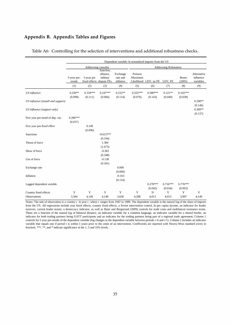
Appendix B. Appendix Tables and Figures

Table A6: Controlling for the selection of interventions and additional robustness checks.

5-year pre-trends

5-year pre fixed effects

Sanction, alliance, military

dispute FEs

Exchange rate and inflation

Poisson Maximum Likelihood LDV, no FE LDV, FE

Bruno (2005)

Alternative influence variables

(1) (2) (3) (4) (5) (6) (7) (8) (9)

US influence 0.230** 0.318*** 0.247*** 0.232** 0.255*** 0.580*** 0.121** 0.102***(0.098) (0.111) (0.084) (0.114) (0.076) (0.143) (0.049) (0.038)

US influence (install and support) 0.298**(0.146)

US influence (support only) 0.309**(0.137)

Five year pre-trend of dep. var. 0.286***(0.037)

Five year pre-fixed effect 0.149(0.096)

Sanctions -0.615***(0.194)

Threat of force 1.300(1.673)

Show of force -0.363(0.348)

Use of force -0.138(0.181)

Exchange rate 0.000(0.000)

Inflation -0.163(0.134)

Lagged dependent variable 0.278*** 0.716*** 0.776***(0.042) (0.034) (0.003)

Country fixed effects Y Y Y Y Y N Y Y YObservations 3,394 4,149 4,149 3,630 4,288 4,013 4,013 3,997 4,149

Dependent variable: ln normalized imports from the US

Addressing causality Addressing Robustness

Notes: The unit of observation is a country c in year t , where t ranges from 1947 to 1989. The dependent variable is the natural log of the share of importsfrom the US. All regressions include year fixed effects, country fixed effects, a Soviet intervention control, ln per capita income, an indicator for leaderturnover, current leader tenure, a democracy indicator, as well as Baier and Bergstrand (2009) controls for trade costs and multilateral resistance terms.These are a function of the natural log of bilateral distance, an indicator variable for a common language, an indicator variable for a shared border, anindicator for both trading partners being GATT participants and an indicator for the trading partners being part of a regional trade agreement. Column 1controls for 5 year pre-trends of the dependent variable (log changes in the dependent variable between periods t -6 and t-1). Column 2 includes an indicatorvariable that equals one if period t is within 5 years prior to the onset of an intervention. Coefficients are reported with Newey-West standard errors inbrackets. ***, **, and * indicate significance at the 1, 5 and 10% levels.

35

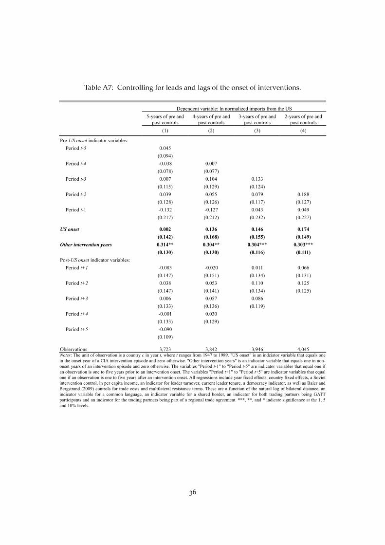
Table A7: Controlling for leads and lags of the onset of interventions.

5-years of pre and post controls

4-years of pre and post controls

3-years of pre and post controls

2-years of pre and post controls

(1) (2) (3) (4)

Pre-US onset indicator variables:Period t-5 0.045

(0.094)Period t-4 -0.038 0.007

(0.078) (0.077)Period t-3 0.007 0.104 0.133

(0.115) (0.129) (0.124)Period t-2 0.039 0.055 0.079 0.188

(0.128) (0.126) (0.117) (0.127)Period t-1 -0.132 -0.127 0.043 0.049

(0.217) (0.212) (0.232) (0.227)

US onset 0.002 0.136 0.146 0.174(0.142) (0.168) (0.155) (0.149)

Other intervention years 0.314** 0.304** 0.304*** 0.303***(0.130) (0.130) (0.116) (0.111)

Post-US onset indicator variables:Period t+1 -0.083 -0.020 0.011 0.066

(0.147) (0.151) (0.134) (0.131)Period t+2 0.038 0.053 0.110 0.125

(0.147) (0.141) (0.134) (0.125)Period t+3 0.006 0.057 0.086

(0.133) (0.136) (0.119)Period t+4 -0.001 0.030

(0.133) (0.129)Period t+5 -0.090

(0.109)

Observations 3,723 3,842 3,946 4,045

Dependent variable: ln normalized imports from the US

Notes: The unit of observation is a country c in year t, where t ranges from 1947 to 1989. "US onset" is an indciator variable that equals onein the onset year of a CIA intervention episode and zero otherwise. "Other intervention years" is an indicator variable that equals one in non-onset years of an intervention episode and zero otherwise. The variables "Period t-1" to "Period t-5" are indicator variables that equal one ifan observation is one to five years prior to an intervention onset. The variables "Period t+1" to "Period t+5" are indicator variables that equalone if an observation is one to five years after an intervention onset. All regressions include year fixed effects, country fixed effects, a Sovietintervention control, ln per capita income, an indicator for leader turnover, current leader tenure, a democracy indicator, as well as Baier andBergstrand (2009) controls for trade costs and multilateral resistance terms. These are a function of the natural log of bilateral distance, anindicator variable for a common language, an indicator variable for a shared border, an indicator for both trading partners being GATTparticipants and an indicator for the trading partners being part of a regional trade agreement. ***, **, and * indicate significance at the 1, 5and 10% levels.

36

Table A8: Testing for FDI and tariff policy mechanisms.

Number of foreign affiliates

Foreign affiliate sales

Foreign affiliate employment ln imports US Tariff change

ln normalized imports from the

US(1) (2) (3) (4) (5) (6)

US influence -0.203 -0.057 0.095 0.332*** 0.003 0.294**(0.189) (0.362) (0.122) (0.120) (0.024) (0.125)

ln (1 + Number of foreign affiliates) -0.037(0.045)

ln (1 + Foreign affiliate sales) 0.022(0.023)

ln (1 + Foreign affiliate employment) 0.066*(0.036)

US influence × Post tariff change 0.026(0.113)

Observations 2,670 2,670 2,670 2,656 2,793 3,885Notes: The unit of observation is a country c, in year t, where t ranges from 1947 to 1989. In columns 1-3, the dependent variables are measures of US FDI. Each ismeasured as the natural log of one plus its value.In columns 4 and 6, the dependent variable is the natural log of imports from the US normalized by total GDP. Incolumn 5, the dependent variable is an indicator variable that equals one if a country changes its tariff schedule in the year. All regressions include year fixed effects,country fixed effects, a Soviet intervention control, ln per capita income, an indicator for leader turnover and a democracy indicator. As well, columns 4 and 6 alsoinclude the Baier and Bergstrand (2009) controls for trade costs and multilateral resistance terms. These are a function of the natural log of bilateral distance, anindicator variable for a common language, an indicator variable for a shared border, an indicator for both trading partners being GATT participants and an indicatorfor the trading partners being part of a regional trade agreement. Coefficients are reported with Newey-West standard errors in brackets. ***, **, and * indicatesignificance at the 1, 5 and 10% levels.

FDI policy channel Tariff policy channel

37