Collision Avoidance for Unmanned Aircraft using Markov Decision...

Collision Avoidance for Unmanned Aircraft using

Markov Decision Processes∗

Selim Temizer†, Mykel J. Kochenderfer‡, Leslie P. Kaelbling§,

Tomas Lozano-Perez¶, and James K. Kuchar‖

Before unmanned aircraft can fly safely in civil airspace, robust airborne collision avoid-ance systems must be developed. Instead of hand-crafting a collision avoidance algorithmfor every combination of sensor and aircraft configuration, we investigate the automaticgeneration of collision avoidance algorithms given models of aircraft dynamics, sensor per-formance, and intruder behavior. By formulating the problem of collision avoidance as aMarkov Decision Process (MDP) for sensors that provide precise localization of the in-truder aircraft, or a Partially Observable Markov Decision Process (POMDP) for sensorsthat have positional uncertainty or limited field-of-view constraints, generic MDP/POMDPsolvers can be used to generate avoidance strategies that optimize a cost function that bal-ances flight-plan deviation with collision. Experimental results demonstrate the suitabilityof such an approach using four different sensor modalities and a parametric aircraft per-formance model.

I. Introduction

Because of the potential for commercial, military, law-enforcement, scientific, and other purposes, un-manned aircraft have received considerable attention in recent years. However, unmanned aircraft are notcurrently permitted access to civil airspace in the United States without special permission from the FederalAviation Administration (FAA). One of the primary concerns with integrating unmanned aircraft is theirinability to robustly sense and avoid other aircraft. Although sensor information can be transmitted to aground pilot who can then maneuver the aircraft to avoid collision, there are concerns about communicationlatency and reliability. In order to provide the high level of safety required by the FAA, an automatedairborne collision avoidance system is likely to be necessary.

The deployment of any collision avoidance system requires a lengthy development process followed by arigorous certification process. Development of the Traffic Alert and Collision Avoidance System (TCAS),currently mandated onboard all large transport aircraft worldwide, started in the 1950s but was not certifiedfor operational use until relatively recently.1 The system issues vertical rate resolution advisories to pilotswho are then responsible for maneuvering the aircraft. TCAS is not certified for autonomous use, and it islikely that the certification of an autonomous system will require even more extensive testing and analysis.

Further complicating the certification process of collision avoidance systems for unmanned aircraft is thediversity of their aircraft performance characteristics and sensor capabilities. Unmanned aircraft can rangefrom under a pound to many tons with wildly varying flight dynamics. Several sensor modalities have beenconsidered for supporting collision avoidance, including electro-optical/infrared (EO/IR), radar, TCAS, andAutomatic Dependent Surveillance-Broadcast (ADS-B). As Table 1 illustrates, these sensor modalities vary

∗The Lincoln Laboratory portion of this work was supported under Air Force Contract #FA8721-05-C-0002. The MITCSAIL portion of this work was supported by the Office of the Director of Defense Research and Engineering. Interpretations,opinions, and conclusions are those of the authors and do not reflect the official position of the United States government.†Ph.D. Student, Massachusetts Institute of Technology, 32-G585, 32 Vassar Street, Cambridge, MA 02139.‡Technical Staff, Lincoln Laboratory, Massachusetts Institute of Technology, 244 Wood Street, Lexington, MA 02420.§Professor of Computer Science and Engineering, Massachusetts Institute of Technology, 32-G486, 32 Vassar Street, Cam-

bridge, MA 02139.¶Professor of Computer Science and Engineering, Massachusetts Institute of Technology, 32-G492, 32 Vassar Street, Cam-

bridge, MA 02139.‖Associate Group Leader, Lincoln Laboratory, Massachusetts Institute of Technology, 244 Wood Street, Lexington, MA

02420.

1 of 22

American Institute of Aeronautics and Astronautics

in their capabilities. It would be very difficult to develop and certify a different collision avoidance systemfor every combination of sensor configuration and aircraft platform. Current efforts in the unmanned aircraftindustry have focused on proprietary solutions for specific platforms and sensors, but a common system thatwould accommodate different sensor configurations and flight characteristics would significantly reduce thecost of development and certification.

Table 1. Qualitative performance characteristics of various sensor modalities. Green, yellow, and red indicate good,moderate, and poor performance, respectively (FoV stands for field-of-view).

Measurement Accuracy Coverage

Modality Range Azimuth Elevation FoV Range Traffic

TCAS

Radar

EO/IR

ADS-B

Such a system would take as input models of the flight dynamics, intruder behavior, and sensor char-acteristics and attempt to optimize the avoidance strategy so that a predefined cost function is minimized.The cost function could take into account competing objectives, such as flight plan adherence and avoidingcollision. One way to formulate a problem involving the optimal control of a stochastic system is as a MarkovDecision Process (MDP), or more generally as a Partially Observable Markov Decision Process (POMDP)to also account for observation uncertainty. POMDPs have been studied in the operations research andartificial intelligence communities, but only in the past few years have generic POMDP solution methodsbeen developed that can approximately solve problems with moderate to large state spaces in reasonabletime. In this work we investigate the feasibility of applying state-of-the-art MDP and POMDP solutionmethods to the problem of collision avoidance.

The experiments we present in this document show that we can model collision avoidance systems usingMDPs, and such systems perform very well in terms of both reducing the risk of collision and having verylittle deviations from the flight plan at the same time, especially with sensors that precisely locate intruderaircraft. We also present experiments with POMDP models built for sensors with limited observationcapabilities that demonstrate how we can still achieve low risk of collision by maneuvering a little more inorder to counterbalance the limitations in observability of intruder aircraft.

The remainder of this document is organized as follows: Section II reviews MDP and POMDP formu-lations and solution methods. Section III presents our parametric aircraft and sensor models. Section IVintroduces the simulation and evaluation framework used to test collision avoidance systems. Sections V,VI and VII describe our collision avoidance models with increasing complexities to handle different sensormodels. Section VIII elaborates on limitations of developed models and suggests ways to improve them.Section IX discusses main conclusions from this work.

II. Review of MDPs and POMDPs

An MDP is a stochastic process where the state of the system changes probabilistically according to thecurrent state and action. POMDPs extend MDPs by including an observation process that probabilisticallygenerates observations conditioned on the current state and action, and hence they have more expressivepower. We will briefly review POMDPs in this section.

The solution to a POMDP is a policy, or way of behaving, that selects actions in a way that takes intoaccount both the current uncertainty about the underlying state of the system (e.g., exact relative positionof the intruder aircraft), as well as future uncertainty about how the system state will evolve (e.g., whatkinds of maneuvers the intruder aircraft will make), by aiming to maximize the expected accumulation ofsome predefined reward (or minimize the expected accumulation of some predefined cost).2 Due to their richdescriptive power, POMDPs have found many uses in computer science and robotics applications such asrobust mobile robot navigation,3 machine vision,4,5 robust dialogue management,6,7 autonomous helicoptercontrol,8,9 and high-level robot control,10 as well as in many other areas like machine maintenance,11 networktroubleshooting,12 medical diagnosis13 and preference elicitation.14 Cassandra provides a comprehensivesurvey of applications utilizing POMDPs.15

Several formulations of POMDPs have been studied in the literature, but this work focuses on the discrete-

2 of 22


time formulation with discrete state and action spaces. We briefly present below a POMDP formulation anddiscuss solution techniques.

II.A. Formulation

In this document, we use S to represent the state space, A to represent the action space, and Ω to representthe observation space, all assumed discrete. The state-transition function T : S × A → Π(S) determinesthe probability distribution over the next states given the current state and action taken. The probabilityof transitioning to state s′ after taking action a from state s is written T (s, a, s′). The observation functionO : S × A → Π(Ω) determines the probability distribution over the observations received after taking someaction resulting in state s′. The probability of receiving observation o after taking action a and landing instate s′ is written O(s′, a, o).

In general, the initial state is unknown. The uncertainty in the initial state is represented by a probabilitydistribution b0 : S → R, where the probability of starting in state s is written b0(s). The space of possiblebeliefs is denoted B. The belief-state b is initialized to b0 and updated with each observation accordingto Bayes’ rule. If the current belief-state is b and action a is taken resulting in an observation o, the newbelief-state b′ is given by

b′(s) = Pr(s′ | o, a, b)∝ Pr(o | s′, a, b) Pr(s′ | a, b)= Pr(o | s′, a)

∑s∈S

T (s, a, s′)b(s)

= O(s′, a, o)∑s∈S

T (s, a, s′)b(s) .

The belief-update process is often referred to as state estimation.Given the current belief-state, the objective is to chose an action that maximizes the expected discounted

return. The discounted return for a sequence of states st and actions at is given by

∞∑t=0

γtR(st, at) , (1)

where γ ∈ [0, 1) is a discount factor and R : S ×A → R is the reward function. The reward for taking actiona from state s is written R(s, a).

The solution to a POMDP is a policy π : B → A that specifies which action maximizes the expecteddiscounted reward given a belief-state. It is known that optimal policies can be represented as a collection α-vectors, denoted Γ. Each α-vector is a vector consisting of |S| components and is associated with a particularaction. The expected discounted return when starting with belief b is

V (b) = maxα∈Γ

(α · b) , (2)

where α · b is the inner product of an α-vector with a vector representation of the belief-state. The functionV is known as the value function. The policy evaluated at belief-state b is the action associated with theα-vector that maximizes the inner product.

II.B. Solution Methods

Finding the collection of α-vectors that represents the optimal policy can be challenging, even for relativelysmall problems. A variety of exact solution methods can be found in the literature, but generally thesemethods do not scale well to large problems. Approximate solution methods generally scale much better andmany of them provide bounds on the regret for the policies they find. The regret of a policy π is the differencebetween the expected discounted return starting at b0 when following π and the expected discounted returnstarting at b0 when following an optimal policy π∗.

In recent years, point-based methods for finding approximate solutions to POMDPs (for example, Point-Based Value Iteration, PBVI16) have received attention because of their ability to solve problems thatare orders of magnitude larger than was previously possible. Point-based methods involve sampling from

3 of 22


the belief space B. In this work we initially used solvers based on Heuristic Search Value Iteration (HSVI2)algorithm.17 We later switched to a solver that uses Successive Approximations of the Reachable Space underOptimal Policies (SARSOP) algorithm18–20 as it performed better on our problems. An implementation ofSARSOP is publicly availablea and we were able to use the software without any modification. SARSOPtakes as input a standard textual representation of a POMDP, including γ, b0, R, T , and O. When theregret bounds fall below some preset value or the user interrupts the solution process, SARSOP outputs apolicy file represented as a collection of α-vectors.

Crucially, although it may require considerable computation to find a near-optimal policy, this work isdone offline. Once a policy has been computed, it can be executed very efficiently online. In the course ofthis work we have developed a new algorithmic technique to make the execution process even more efficient,making it entirely suitable for execution online, in real time, on an aircraft.

III. Aircraft and Sensor Models

The aircraft model we developed for our collision avoidance systems is parametric and can be modifiedto mimic different types of aircraft. In our implementation, parameter values are based on Global Hawk, anunmanned aerial vehicle (UAV) used by the United States Air Force as a surveillance aircraft. Table 2 showsperformance limits for Global Hawk. Our collision avoidance models use a subset of these values; maximumand minimum velocities and maximum climb/descent rates.

Table 2. Global Hawk performance limits.

Maximum velocity 180 kts

Minimum velocity 100 kts

Maximum climb rate 3500 fpm

Maximum descent rate 4000 fpm

Maximum bank angle 35 deg

Maximum bank rate 8 deg/s

Maximum pitch rate 2 deg/s

Maximum turn rate 2.5 deg/s

Before describing our sensor models, let us introduce four coordinate systems shown in Figure 1 that wewill refer to in the rest of this document:

• Global Coordinate System (GCS): This coordinate system is also known as the Earth CoordinateSystem. The origin is an arbitrary point chosen by the model simulation and evaluation framework.Positive x is east, positive y is north, and positive z is altitude.

• Local Coordinate System (LCS): The origin of LCS is ownship center of mass (i.e., LCS is anegocentric coordinate system). Positive x is in the direction of the right wing, positive y is the directionof the nose, and positive z is upwards.

• Auxiliary Coordinate System (ACS): This is also an egocentric coordinate system whose x-y-zaxes are aligned with the east-north-altitude axes of GCS, respectively.

• Relative Coordinate System (RCS): This is another egocentric coordinate system which is obtainedby rotating ACS around its z axis until the y-z plane intersects with intruder aircraft center of mass.RCS is a 2-dimensional coordinate system. The x and y axes of RCS are the y and z axes of the rotatedACS, respectively. The RCS is also referred to as the projection plane.

Input to our collision avoidance systems may come from various sensors with different characteristicsand sensing ranges (usually expressed by radii in nautical miles, NM ) onboard the UAV. We developed fourdetailed sensor models that are capable of simulating following types of erroneous measurements and noise:

• False positive measurements: We may detect an intruder when, in fact, there is no intruder aircraftin the sensor range (for example, a bird in sensing range might cause false positive measurements).

aM2AP Research Group at NUS, POMDP Planning, http://motion.comp.nus.edu.sg/projects/pomdp/pomdp.html (Decem-ber 2009).

4 of 22


Global Coordinate System Local Coordinate System

Auxiliary Coordinate System Relative Coordinate System

Figure 1. Coordinate systems.

• False negative measurements: We may fail to detect an intruder when one is present in the sensorrange.

• Measurement errors: We may detect the intruder aircraft in a position or at an angle that is notcorrect.

The probabilities of false positive and false negative measurements (pfp and pfn) are usually specific todifferent sensor hardware, and the measurement errors are computed according to realistic error models.

The four sensor models studied in this research are as follows:

1. Perfect sensor: This is a hypothetical omnidirectional sensor with no noise and no false posi-tive/negative detections (pfp = pfn = 0). The sensor reading consists of east, north and altitudecoordinates of intruder aircraft in GCS. With this sensor, it is possible to localize intruder aircraft toan exact point in either GCS or LCS.

2. TCAS sensor: This is a model of the actual TCAS sensor.21 It is based on listening to transponderreplies from nearby aircraft and is omnidirectional. It provides bearing in LCS, altitude in GCS,and range (the line-of-sight distance between ownship and intruder aircraft, also referred to as slantrange). The error in range measurement is Gaussian with zero mean and 50 ft standard deviation. Theerror in bearing estimate is Gaussian with zero mean and 10 deg standard deviation. The altitude ofintruder aircraft is measured with 25 ft quantization. There is also an altimetry error bias that remainsconstant during an encounter with an intruder aircraft, and is Laplacian with zero mean and 40 ft scale.Probability density function for the Laplace distribution is shown in Figure 2. In the TCAS sensormodel, pfp = 0 (since detection is based on broadcast signals) and pfn = 0.01. With a noiseless TCASsensor, intruder aircraft could be localized to a point in LCS, but considering the given error model,the region that the intruder could be residing in has approximately the shape of a distorted truncatedspherical cone.

5 of 22


Figure 2. Probability density function for the Laplace distribution (location = 0, scale = 40).

3. Radar sensor: Our radar sensor model has a limited field-of-view (FoV), ±15 deg elevation and ±110azimuth. It provides bearing and elevation readings in LCS, and range and range rate information.As with TCAS, the error in the range measurement is Gaussian with zero mean and 50 ft standarddeviation. Range rate error is Gaussian with zero mean and 10 ft/s standard deviation. The error in thebearing estimate is Gaussian with zero mean and 10 deg standard deviation. Elevation error estimateis Gaussian with zero mean and 1 deg standard deviation. For the radar sensor, pfp = pfn = 0.01.Intruder aircraft can be localized approximately into a distorted truncated spherical cone in LCS.

4. Electro-optical/infrared (EO/IR) sensor: Our EO/IR sensor model is very similar to the radarsensor with less angular measurement noise and without a range reading. It has a limited FoV,±15 deg elevation and ±110 azimuth. Sensor reading consists of bearing and elevation angles in LCS,and line-of-sight rate information. Error in both angular measurements is Gaussian with zero mean and0.5 deg standard deviation. Line-of-sight rate error is Gaussian with zero mean and 0.5 deg/s standarddeviation. For the EO/IR sensor, pfp = pfn = 0.01. Intruder aircraft can be localized approximatelyinto a distorted spherical cone in LCS.

Parameters are given in Table 3, and sensor capabilities are summarized in Table 4.

IV. Simulation and Evaluation Framework

The performance of our collision avoidance systems were evaluated using a simulation framework devel-oped for prior TCAS studies22 and sense-and-avoid systems for unmanned aircraft.23 We used an encountermodel derived from 9 months of national radar data24 to generate 15,000 scripted encounters between pairsof aircraft and allowed our collision avoidance systems to control of one of the aircraft. For comparison,we evaluated the performance of other collision avoidance systems to baseline performance. This sectiondescribes our simulation and evaluation process.

IV.A. Simulation Framework

Figure 3 provides an overview of the simulation framework. An encounter model is used to generate initialconditions and scripted maneuvers for both aircraft involved in the encounter. These initial conditions andscripts are fed into a 6 degree-of-freedom, point-mass dynamic model. The sensor model takes as inputthe current state from the dynamic model and produces an observation, or sensor measurement. The stateestimation process updates the belief-state based on the observation. The MDP/POMDP policy is evaluatedon the updated belief-state and an optimal, or approximately optimal, action is executed. The dynamic modelupdates the state, and the process continues until the end of the encounter.

IV.B. Baseline Collision Avoidance Systems

We compared the performance of our system against the following three baseline systems:

6 of 22


Table 3. Complete list of sensor parameter values.

Perfect

Range 5 NM

False positive measurement probability 0.00

False negative measurement probability 0.00

TCAS

Range 5 NM

Altitude quantization 25 ft

Range error standard deviation 50 ft

Bearing error standard deviation 10 deg

Altimetry error scale 40



Radar

Range 5 NM

Minimum azimuth −110 deg

Maximum azimuth 110 deg

Minimum elevation −15 deg

Maximum elevation 15 deg

Range error standard deviation 50 ft

Bearing error standard deviation 1 deg

Elevation error standard deviation 1 deg

Range rate error standard deviation 10 ft/s



EO/IR

Range 5 NM

Minimum azimuth −110 deg

Maximum azimuth 110 deg

Minimum elevation −15 deg

Maximum elevation 15 deg

Bearing error standard deviation 0.5 deg

Elevation error standard deviation 0.5 deg

Line-of-sight rate error standard deviation 0.5 deg/s



Table 4. Sensor capabilities. Green, yellow, and red indicate good, moderate, and poor performance, respectively.

Perfect TCAS Radar EO/IR

Range

Bearing

Altitude

Elevation

Range rate

Line-of-sight rate

Position

7 of 22


SensorModel

StateEstimation

PolicyEvaluation

DynamicModel

EncounterModel

s

o b

scripta

Figure 3. Simulation framework.

• TCAS Version 7: The TCAS Version 7 system uses only the TCAS sensor readings as input. Thebehavior of this system is as specified in the TCAS II standard.21

• Basic Collision Avoidance System (Basic CAS): It is possible to use all four sensor models withBasic CAS, but the performance decreases severely with the limited field-of-view sensors. The collisionavoidance logic is very simple: If an intruder aircraft is detected inside the sensing region, and theprojection of the intruder position on RCS has a positive y value (i.e., the intruder is “above”), thenownship accelerates down with 0.25 g until next observation is received. Similarly, if the intruder is“below” (projection of its position on RCS has a negative y value), then ownship accelerates up with0.25 g until the next observation.

• Analytic Collision Avoidance System (Analytic CAS): Analytic CAS is based on collectingposition data for ownship and intruder aircraft, and estimating their motion (velocities and accelera-tions) in full 3-dimensional coordinates by simple differentiation. Therefore, it is best suited for usewith perfect and TCAS sensors, which are omnidirectional, have none or very little noise (comparedto other sensor models) and hence allow the intruder to be localized with high accuracy at each simu-lation step. The collision avoidance logic works as follows: Based on regularly collected and updatedposition, velocity and acceleration estimates, a clear-of-danger test is performed using simple quadraticequations of motion at each simulation step. If there is no danger of a collision or a close encounter inthe future, ownship continues to follow the scripted maneuver, but if the test fails (i.e., the minimumdistance between the extrapolated trajectories of both aircraft is below some threshold), an evasivemaneuver is performed, which is simply to increase ownship’s altitude by 200 ft as quickly as possiblewithin the performance limits. After the maneuver is completed, the collision avoidance logic resumestests and triggers further evasive maneuvers as necessary. We implemented two versions of the clear-of-danger test: The first version, called Analytic CAS 1-D, checks if only the vertical distance betweentwo aircraft will drop below a threshold, and the second version, called Analytic CAS 3-D, checks ifthe intruder will invade a predefined 3-D volume surrounding ownship (which is usually in the shapeof a hockey puck that is 200 ft thick and 1000 ft in diameter).

V. Perfect Sensing

The first case we will consider is sensing with no noise, and for that purpose we will assume that ownshipis equipped with a perfect sensor. When there is no observation uncertainty, we can model the collisionavoidance system as an MDP. Note that we allow uncertainty about the behavior of the intruder aircraft,and MDP formulation lets us capture this uncertainty in the state-transition model. In this section, we willlook at the general structure of the state and action spaces and the details of the reward and state-transitionmodels that will compose our MDP collision avoidance system.

V.A. MDP Collision Avoidance System

The true state space model in the collision avoidance problem is continuous and consists of the followingcomponents for both aircraft present in the encounter:

• Position specified in GCS

• Orientation specified as yaw, pitch and roll angles

8 of 22


• Air speed, air speed acceleration

• Vertical rate, vertical acceleration

• Yaw rate, pitch rate and roll rate

This set of components is referred to as the aircraft state vector. This is a very high-dimensional contin-uous space (26 dimensions for both aircraft together). The action space for a UAV is also continuous as itis possible to choose and apply any vertical and/or horizontal accelerations within ownship’s performancelimits.

In this work, we consider a simplified version of the problem in which ownship can only maneuververtically, but not in azimuth, to evade intruders, similar to TCAS II. We also work with discretized spaceswith less number of dimensions that are carefully selected to incorporate important information from thetrue spaces.

V.A.1. State Space

The size of a discretized state space is exponential in the dimension and in the case of 26 dimensions, wecould not stand to have even two discrete values per dimension. So, before we discretize the state space, wemust first represent it in a much lower-dimensional subspace that captures the essence of the encounter.

To encode relative positions and velocities of the aircraft, we chose RCS as our main representation. Inthis coordinate system, the state consists of the following components:

• X: horizontal distance from ownship to intruder aircraft;

• Y : vertical distance from ownship to intruder aircraft;

• RelativeVx: (relative) velocity in X, representing the horizontal closure rate;

• OtherVy: vertical velocity of intruder aircraft; and

• OwnVy: vertical velocity of ownship.

This 5-dimensional state space is discretized by dividing each dimension into a finite number of bins. Thesizes of the bins may be non-uniform. The overall state-space is then a set of 5-orthotopes (5-dimensionalboxes or hyperrectangles) that exhaust a continuous piece of the overall 5-dimensional state space. Weaugment the state space with two sets of special states: start states and done states. These states are usedto model situations when the state space is initialized (and the encounter has not started), and when theencounter is over, respectively. Because the vertical velocity of ownship is always known, we always includeit in the state space. So, the start and done state sets both contain a member for each bin of OwnVy,modeling flight at some vertical velocity before the start of or after the termination of, an encounter. Havingdiscretized the state space in this way, a state may be represented simply as an index into the set of boxesspanning the space, or an index to one of the start or done states.

V.A.2. Action Space

We adopted a simple discrete action-space model that consists of commands to ownship to apply positiveor negative fixed vertical accelerations for a fixed duration (usually 1 s). For the MDP CAS, our actionspace consists of 17 uniform samples from the ±8 ft/s2 (±0.25 g) acceleration range imposed by the aircraftperformance limits; A = −8,−7, · · · ,−1, 0, 1, · · · , 7, 8. It is possible to sample the range of verticalaccelerations more densely, but the solvers would require more time to find policies with tight regret bounds.

V.A.3. Reward Model

The reward function in our MDP formulation is in the form of costs (or negative rewards) rather thanpositive rewards. It is designed with the following three objectives in mind:

9 of 22


• As the primary goal of the collision avoidance algorithm, the intruder aircraft should never occupythe same bin as ownship in the RCS, which implies a collision or a very dangerous encounter. Notethat ownship resides at the origin of the RCS, and it is possible that the origin might be on the edgeor vertex of one or more bins rather than being inside a single bin due to the chosen vertical andhorizontal division strategy. In that case, the collision avoidance algorithm should prevent the intruderfrom moving into any one of the bins that have any boundaries touching the origin.

• In addition to preventing collision, it is desirable to maintain some protected airspace around ownshipwhere the intruder aircraft should not penetrate. This protected airspace is specified by two parameters:a vertical separation range and a horizontal separation range. In our tests for MDP CAS, we used 100 ftvertical and 500 ft horizontal separation ranges, same as that of the NMAC definition used in priorTCAS safety studies.25–28 The second goal of the collision avoidance algorithm should be to preventother aircraft moving into any bin that has some parts overlapping with the protected airspace.

• As the last goal, if there is no danger of collision or penetration of protected airspace, ownship shouldlevel off and try to maintain a zero vertical velocity. It may be argued that ownship should try toreturn to its commanded flight path. We have taken the position that, during the handling of a closeencounter, it is enough to prefer level flight, and that after the encounter is over, standard navigationalprocedures can be resumed.

In order to satisfy these goals, the reward may be specified as a function of the state of the system. It isspecified using three user-defined parameters:

• Collision cost: The cost of any state in which the intruder is in the same X and Y bins as ownship,currently set to −1000;

• Protected airspace violation cost: The cost of any state in which the intruder aircraft is withinthe protected airspace region in X and Y , currently also set to −1000; and

• Vertical velocity penalty: The cost for being in a state where the OwnVy bin does not contain0 ft/s; for the MDP CAS, vertical velocity penalties are linearly proportional to the velocity valuesthat correspond to the centers of the OwnVy bins. It is possible to vary the maximum penalty valuein order to reach different equilibria in balancing evasive maneuvers and level flight.

All other states are assumed to have a reward of 0. Note that the solution to the MDP will remain thesame for any linear scaling of reward values, so only the relative magnitudes have an effect.

V.A.4. State-Transition Model

The initial state distribution specifies that the system starts in a uniformly chosen start state. At eachstep, an action is taken and the probability distribution over the state space is updated according to thestate-transition model.

Our assumption is that there is no actual stochasticity in the dynamics of the system. However, we modelthe uncertainty in intruder behavior as a random process; and the fact that the state space is discretized willintroduce uncertainty in the transitions, even though they are governed by a deterministic physical process.

Our state-transition model is characterized by the following parameters:

• Controller frequency, ∆T : Duration between successive consultations of the MDP policy for choosingan action. This value is used by the MDP formulation to predict what the state will be in the nextiteration.

• Magnitude of our vertical acceleration, OwnAy.

• Our vertical velocity limits, OwnVyMin and OwnVyMax.

• Probability of staying in start state when already in start state.

• Probability of making a transition into any other state when in start state.

• Intruder aircraft’s horizontal and vertical acceleration models.

10 of 22


For the horizontal and vertical acceleration models, we used the distributions given in Table 5. Thesedistributions roughly model a random walk process where the intruder aircraft is oblivious to ownship or wehave no idea about the intention of the intruder aircraft.

Table 5. Horizontal and vertical acceleration models for intruder aircraft.

Horizontal Model

v (ft/s2) Probability

−300.0 0.05

−200.0 0.05

−100.0 0.05

−30.0 0.10

−20.0 0.10

−10.0 0.10

0.0 0.10

10.0 0.10

20.0 0.10

30.0 0.10

100.0 0.05

200.0 0.05

300.0 0.05

Vertical Model

v (ft/s2) Probability

−10.0 0.1

−5.0 0.2

0.0 0.4

5.0 0.2

10.0 0.1

Given these parameters, we compute Pr(s′ | s, a) as follows:

• First, we consider each possible pair of vertical and horizontal accelerations ao that might be chosenby the intruder aircraft, and compute their probabilities po as the product of the probabilities in theintruder acceleration models.

• For each vertex of the bin s, we determine how that particular point in state space would be transformedgiven the execution of ownship acceleration a, and the intruder accelerations ao.

• The result is a new box, B, in 5-dimensional space. For each new state s′, we compute the percentageof B that overlaps s′; that overlap percentage is Pr(s′ | s, a, ao). Any probability mass outside theboundaries of the modeled state space is assigned Pr(done ,OwnVy | s, a, ao).

• Finally,Pr(s′ | s, a) =

∑a0

Pr(s′ | s, a, ao)po .

This method of computing the physical evolution of the system analytically eliminates introducing addi-tional discretization in the computation. Therefore, the effectiveness of the state-transition model dependsonly on the discretization of the state and action spaces and the fidelity of the vertical and horizontal accel-eration models for the intruder aircraft. Having the acceleration models match closely to the actual intruderbehaviour results in better state estimations, where the intruder aircraft would be localized more accurately.

V.B. Results

Table 6 summarizes the results of nominal flight (ownship following the scripted flight path without usingany collision avoidance systems) and baseline collision avoidance systems on 15,000 encounters. The tableshows the risk ratios, mean vertical velocity magnitudes in ft/s, and mean vertical acceleration magnitudesin ft/s2 for different algorithms. The risk ratio associated with a particular system is the probability that anencounter leads to an NMAC using the system divided by the probability that an encounter leads to an NMACwithout the system. Of course, better performance is indicated by a small risk ratio. It is desirable to havevelocity and acceleration values as small as possible without sacrificing the risk ratio. Large values of meanvelocity magnitude and mean acceleration magnitude indicate that ownship is maneuvering unnecessarily.

We experimented with gradually increasing the size of the state space (by increasing the number of binsalong different dimensions in our discretization) until the time it takes for the solver to compute a policyincreases beyond practical limits, and we ended up with an MDP model with 6768 states: 5, 10, 3, 5 and9 bins for X, Y , RelativeVx, OtherVy and OwnVy components of S, respectively, and 9 start and 9 done

11 of 22


Table 6. Risk ratios for nominal flight and baseline collision avoidance systems.

Ratio Velocity Acceleration

Nominal 1.000000 4.255460 0.172020

TCAS II (2500 ft/min) 0.061220 5.094360 0.345920

TCAS II (1500 ft/min) 0.062730 4.586190 0.366110

Basic CAS (perfect sensor) 0.000010 33.030760 0.790190

Analytic CAS, 3-D (perfect sensor) 0.054560 4.564330 0.224730

Analytic CAS, 1-D (perfect sensor) 0.016970 5.597470 0.768990

states. Solving an MDP using value iteration29 is very efficient especially if the solver is implemented usingsparse data structures. Therefore, instead of testing a single instance of an MDP, we were able to varythe vertical velocity penalty (reward) and generate multiple instances of our MDP CAS model to trace outsystem performance (SP) curves. SP curves are similar in nature to system operating characteristic (SOC)curves,30–32 which generally involve plotting unnecessary alert against successful alert. Results for our MDPCAS is given in Table 7 and Figure 4 shows SP curves pertaining to our MDP model. In the SP curves,points close to the origin are more desirable as they represent low risk ratios and low velocity/accelerationvalues (less maneuvering), and our MDP model scores better than the other systems on the Velocity - RiskRatio curve.

Table 7. Risk ratios for MDP collision avoidance system (perfect sensor).

Reward Ratio Velocity Acceleration

−0.10 0.000692 14.174462 2.121009

−0.50 0.000980 7.721526 1.684897

−0.75 0.001428 5.505732 1.745723

−1.00 0.003075 4.970565 1.591075

−1.25 0.022785 4.133050 1.566663

−1.50 0.024709 3.820564 1.286228

−2.00 0.036734 3.125315 0.931763

−5.00 0.063469 2.159921 0.691902

−10.00 0.170806 1.460390 0.539181

−20.00 0.257840 1.059476 0.241147

−30.00 0.431986 0.973162 0.212496

Velocity vs. Risk ratio. Acceleration vs. Risk ratio.

Figure 4. System performance curves for MDP collision avoidance system.

Graphs displaying velocity, acceleration and probability of NMAC (PNMAC) values from 15,000 en-counters using nominal flight strategy plotted against values from same encounters using our MDP collisionavoidance logic are shown in Figure 5. In these graphs, scoring below the (red) diagonal are desirable as itindicates that an aircraft equipped with our collision avoidance system performs better (in terms of lower

12 of 22


risk ratio or less maneuvering) than an aircraft that just follows the scripted maneuver for that particularencounter scenario. Note that our reward model is constructed to optimize velocities, therefore accelerationplots are not significant for our experiments in general, but presented as a reference. Also, in the PNMACcomparison, there are a few encounters where the MDP PNMAC is higher than Nominal PNMAC (pointsabove the diagonal), which means that the collision avoidance system actually increased the risk ratio. Thiscan happen in the following case: intruder aircraft performs a dangerous altitude crossing maneuver thathappens to have a large miss distance when ownship follows the scripted maneuver, but the miss distanceis small when ownship follows the commands from the collision avoidance system that is trying to avoid thesame dangerously close intruder where the intruder behavior is modeled by a random walk process.

Nominal vs. MDP CAS - Velocity Nominal vs. MDP CAS - Acceleration

Nominal vs. MDP CAS - PNMAC

Figure 5. Velocity, acceleration and PNMAC graphs, Nominal vs. MDP CAS.

Since our reward model is constructed with penalizing high vertical velocities as our goal, it is notsurprising that we do not get low acceleration values as opposed to the optimization we get with velocities.In fact, the MDP CAS prefers using high acceleration values. The histogram in Figure 6 shows the totalnumber of states an action is chosen as the best action by the MDP policy (this specific policy was generatedwith vertical velocity penalty = −2.00).

In conclusion, we can say that MDP CAS works well in the case of perfect sensing, and we can easilyoutperform baseline collision avoidance systems in terms of much lower risk ratios and velocities (withoutunnecessary maneuvering).

VI. Noisy Sensing

Our second case is omnidirectional sensing with noise, and we will use the TCAS sensor model as ourinput source. If we were to make use of the bearing estimate produced by the TCAS sensor in locating theintruder aircraft in any 3-dimensional coordinate system, the error might be considerably big (especiallywith distant intruders). However, we chose to work with projections of intruder aircraft on RCS and hence

13 of 22


Figure 6. Frequencies of best actions in MDP policy (vertical velocity penalty = −2.00).

we do not need the bearing estimate at all. It is possible to accurately locate the intruder on RCS usingother TCAS readings. This gives us the following two options in designing a collision avoidance system thatuses the TCAS sensor:

• We treat this as a perfect sensing problem and use the same MDP model developed in Section V. Tofigure out the state, we either directly use the sensor reading neglecting the fact that it is noisy, or weuse an estimator such as an alpha-beta tracker33 or a Kalman Filtering based technique.34 Since smallobservation noise does not affect action selection much in this specific problem, an alternative to usingan external state estimator is to formulate the problem as a QMDP.35

• We define a discretized observation space Ω, and design an observation model for the TCAS sensor toaugment the MDP model of Section V, and turn the problem into POMDP planning.

In this section, we first present results for an MDP collision avoidance model using an alpha-beta trackerto estimate the state, and then we look at a POMDP model.

VI.A. MDP Collision Avoidance System with State Estimator

The results for baseline collision avoidance systems with the TCAS sensor are shown in Table 8. Using asimple alpha-beta tracker for state estimation with α = β = 0.5, we obtained the results in Table 9 withour MDP collision avoidance system for various vertical velocity penalty values. The SP curves are shownin Figure 7.

Table 8. Risk ratios for baseline collision avoidance systems (TCAS sensor).


Basic CAS (TCAS sensor) 0.000010 32.909700 1.034700

Analytic CAS, 3-D (TCAS sensor) 0.080100 7.402750 1.096570

Analytic CAS, 1-D (TCAS sensor) 0.020500 19.557490 4.511640

Even though alpha-beta tracking is a very simple state estimation method, the results are satisfactory.Using Kalman filters, interacting multiple model methods,36 or nonlinear filters37 may further improve thequality of state estimation.

VI.B. POMDP Collision Avoidance System with TCAS Sensor

The state space S, and the state-transition model we built in Section V effectively capture important aspectsof the encounter geometry and motion dynamics for both aircraft, respectively. Therefore, a POMDP collisionavoidance model can be built on top of the MDP model of Section V by just adding an observation model.In this section, we will define the observation space and the observation model for the TCAS sensor, and wewill also look at how we can slightly modify action space and reward model together to reduce the POMDPsize and still obtain low risk ratios.

14 of 22


Table 9. Risk ratios for MDP collision avoidance system (TCAS sensor).

Reward Ratio Velocity Acceleration

−0.10 0.000916 13.225057 3.088738

−0.50 0.001717 7.431411 2.404085

−0.75 0.002428 5.101627 2.398184

−1.00 0.003337 4.494725 2.151822

−1.25 0.015149 3.857991 1.967395

−1.50 0.023313 3.657201 1.618871

−2.00 0.037456 2.906691 1.221383

−5.00 0.077662 2.033404 0.902261

−10.00 0.212924 1.448597 0.576285

−20.00 0.285638 1.055002 0.284902

−30.00 0.415815 0.993773 0.243202

Velocity vs. Risk ratio. Acceleration vs. Risk ratio.

Figure 7. System performance curves for MDP collision avoidance system.

15 of 22


VI.B.1. Observation Space

The discrete model of the observation space is constructed in a way similar to the discrete state space.There are two types of observational information: vertical velocity of ownship (OwnVy, which we assume isalways completely and correctly observed), and possible single detection of an intruder aircraft using a sensorsystem. Observations for the TCAS sensor are discretized into the same bins as the X and Y components ofthe state space. The model could easily be changed to provide observations at a higher or lower granularity.In addition, there is a special noObs observation for the case when no intruder is detected (due to either anempty sensing region or a false negative measurement).

VI.B.2. Observation Model

The observation model of a POMDP specifies Pr(o | s, a), that is, the conditional probability of making eachpossible observation o, given that the actual state is s and the last action was a. All necessary informationis encapsulated in s, so we will ignore dependence on a, and specify Pr(o | s) for all discrete o and s.

We assume that, at every step, the observation has two components: oovy , our measured vertical velocity,and od, the observed detection of the intruder, and that these are independent, so

Pr(oovy , od | s) = Pr(oovy | s) Pr(od | s) .

The measurement of our vertical velocity is always correct, so Pr(oovy | s) = 1 if oovy is equal to theOwnVy component of s, and 0 otherwise.

The observed detection is more complex due to false positive/negative measurements and measurementerrors described in Section III. We assume fixed probabilities for false positives pfp and false negatives pfn ,and assume that if there is a false positive detection, it is generated with uniform probability over the spaceof values of od.

When s is a start or done state (the encounter has not yet begun or has terminated) or when Y >maxRange, that is, when the distance to the other aircraft is greater than the range of the sensor, thenPr(od = noObs | s) = 1− pfp . That is, with high probability, the observation is noObs. We used a value of5 nautical miles for maxRange for all sensors. For any other observation Pr(od = d | s, fp) = |Od|−1; that is,it is uniform over the space of possible actual detection observations.

Finally, if the intruder is within the modeled volume of the state space, there is some chance of not seeingthe intruder: Pr(od = noObs | s) = pfn . Otherwise, with probability 1− pfn , we make a detection d.

A precautionary margin is added to all four sides of the X,Y rectangle corresponding to the detection d.Then we consider all of the X,Y bins bi that overlap the expanded detection bin, and the proportion of theexpanded detection bin that overlaps bi, called pi. So,

Pr(od = d | s) = (1− pfp)pi + pfp|Od|−1 ,

for any state in which the intruder is in X,Y bin bi, for all bins bi, and

Pr(od = d | s) = pfp|Od|−1

otherwise. For the TCAS sensor, we can define the margin in terms of standard TCAS sensor error parametersgiven in Table 3:

margin = Altitude quantization +3× Range error standard deviation +3×Altimetry error scale

Including full altitude quantization and 3 standard deviations worth of error in the margin gives usan unnecessarily conservative confidence region around the detection d which can, in fact, hinder intruderlocalization and render the observation model useless. The margin should be large enough so that it coversthe region from which a noisy sensor reading may have originated, but it should be small enough to allowthe POMDP to properly localize the intruder. Therefore, we used smaller margins in our experiments (halfof altitude quantization and 0.5 standard deviations gave us reasonable risk ratios).

16 of 22


VI.B.3. Modifications

POMDP solvers work with belief-states instead of exact states and branch on actions and observations,therefore their memory and time demands are typically much higher than MDP solvers, especially if wewould like to compute policies with tight regret bounds. A POMDP model with the same state and actionspaces as the MDP model of Section V takes days to just initialize and generate the first heuristic policyin the iterative improvement process. We describe below how the parametric design of our POMDP modelgave us leverage to reduce the size without decreasing performance.

As depicted in Figure 6, the MDP collision avoidance logic mostly uses very high, very low or zeroacceleration options available when picking an action. This is in accordance with our reward model. Basedon this observation, we used a new and smaller action space with only three actions, A = −8, 0, 8, whichcorrespond to accelerating up/down with maximum magnitude or maintaining vertical velocity.

We also used a slightly different discretization for the state space: 7, 10, 4, 4 and 3 bins for X, Y ,RelativeVx, OtherVy and OwnVy components of S, respectively, and 3 start and 3 done states, whichbring the number of states down to 3366.

Based on some experimental results, we modified the reward model as follows: we increased the size of theprotected airspace around ownship to 200 ft vertical and 1000 ft horizontal separation, and we set protectedairspace violation cost to −500.

These modifications let the SARSOP solver initialize in about an hour and generate acceptable policies(in terms of low risk ratios) in 3 to 5 hours.

VI.C. Results

Tracing out SP curves for POMDP models is very time consuming, and essentially the more the solver runs,the better the generated policies perform. Therefore, we present the single best result we obtained for ourPOMDP model (in terms of low risk ratio) using a vertical velocity penalty of −0.1 in Table 10. The POMDPcollision avoidance logic for the TCAS sensor is about 20 times safer than TCAS Version 7 currently usedon manned aircraft. However, TCAS has a much lower mean vertical velocity magnitude, indicating that itmaneuvers less frequently.

Table 10. Risk ratio for POMDP collision avoidance system (TCAS sensor).


POMDP CAS (TCAS sensor) 0.002770 14.133030 1.759190

Although we use the same sensor model of the TCAS algorithm for our POMDP model and constrainthe vertical rate magnitude to be within 2500 ft/min, the comparison is not entirely fair. TCAS wasdesigned for pilot-in-the-loop control and assumes a delay between when the resolution advisory is issuedand when the pilot responds. Although the POMDP algorithm has the advantage over the TCAS algorithmbecause it can maneuver instantaneously, the TCAS algorithm is permitted to make up to 0.35 g maneuverswhereas the POMDP was constrained to 0.25 g maneuvers. We use the standard model of pilot responseto TCAS resolution advisories, which is a 0.25 g acceleration after a 5 s delay for the initial advisory and a0.35 g acceleration after a 2.5 s delay for subsequent advisories.38 Although a direct comparison between thePOMDP model and TCAS algorithm cannot be made, we can be confident, at least, that the POMDP isperforming well.

Considering the MDP model results and comparing both risk ratio and flight plan adherence, we concludethat, for the TCAS sensor, an MDP model is the right choice.

VII. Limited Field-of-View Sensing

As our final case, we look at POMDP collision avoidance using radar and EO/IR sensors. Both of thesesensors have noise, and are effective only within a limited sensing region. Most important complicationscaused by these two sensors are the following:

• Unlike the TCAS sensor which provides an accurate altitude reading in GCS, these sensors provideelevation estimates that we need to use when projecting the intruder aircraft location on RCS. Usingan angular measurement makes it difficult to localize distant intruders in RCS, so until the intruder is

17 of 22


sufficiently close, the altitude estimate will not help the POMDP model much in choosing an evasiveaction.

• The sensing region is horizontally wide, but vertically, it is a very narrow band in front of ownship.Therefore, nearby aircraft can fly undetected most of the time (even when they are dangerously close).This also causes late detection of some ascending or descending intruders that suddenly enter thedetection region, leaving very little space and time for an escape maneuver.

• During an escape maneuver, the sensor orientation (and hence the orientation of the detection region)changes as ownship accelerates (pitches) up or down. Most of the vertical maneuvers cause the intruderto move outside of the sensing region.

In terms of model implementation, there is very little work to do: We base our design on the POMDPmodel of Section VI.B (using the same state and action spaces described in Section VI.B.3) with some minoradjustments that we describe below, we use the previously introduced special observation, noObs, wheneverthere is no detection (for example, when a state falls outside sensing region), and we just employ the POMDPsolver to design effective strategies for dealing with the limitations of sensing. This also validates one ofour central premises for this work; POMDP models allow us to easily and quickly design collision avoidancestrategies for different sensor configurations.

VII.A. POMDP Collision Avoidance System with Radar Sensor

For the radar sensor, we use the same observation model as the TCAS sensor with the following two modi-fications:

• An overly conservative margin can be defined in terms of standard error parameters from Table 3:

margin = 3× Range error standard deviation +Longest distance to bin edges× tan(3× Elevation error standard deviation)

• The pitch angle of ownship (and hence the orientation of the sensing region) can be computed usingownship’s vertical and horizontal velocity values, but ownship horizontal velocity is currently not partof the state space. In our observation model implementation, we compute some very loose upper andlower bounds for pitch angle using the maximum and minimum velocities of our aircraft model fromTable 2, and use them to figure out which X,Y boxes fall outside sensing region. We believe thatperformance could further be improved with a better POMDP model that could accurately predict thefield-of-view of the sensor. However, addressing this issue requires an extension to the state space andincreases the POMDP size considerably.

VII.B. POMDP Collision Avoidance System with EO/IR Sensor

The EO/IR sensor reports the elevation angle of the intruder aircraft, therefore the projection of the intruderon RCS can be constrained to lie on a ray (with noise) rather than a point.

Detections from the EO/IR sensor are nominal angles that can be thought of as the centers of angularbins, which are not necessarily uniform. For each state s in which the intruder is located in the modeledX,Y space, we can compute a nominal elevation angle d∗(s) to the intruder. We assume that the probabilityof observing a detection angle d when the actual angle is d∗ is proportional to a Gaussian density with meanat d∗; so,

Pr(od = d | s) = (1− pfp)1ze(d−d∗(s))2 + pfp|Od|−1 ,

wherez =

∑s

e(d−d∗(s))2

is the normalization constant.We also use the same pitch angle approximation of the radar sensor described in Section VII.A to assign

noObs to X,Y boxes that fall outside the sensing region.

18 of 22


VII.C. Results

Table 11 summarizes results for baseline and POMDP collision avoidance systems using radar and EO/IRsensors. The vertical velocity penalty was set to −0.1 for the POMDP models.

Table 11. Risk ratios for baseline and POMDP collision avoidance systems (radar and EO/IR sensors).


Basic CAS (radar sensor) 0.050830 19.232450 2.409710

Basic CAS (EO/IR sensor) 0.047240 19.450350 2.308330

POMDP CAS (radar sensor) 0.063370 23.628310 1.261540

POMDP CAS (EO/IR sensor) 0.035100 28.610760 1.476910

As expected, radar and EO/IR sensors have higher risk of collision than TCAS and perfect sensors sincetheir performance is inherently limited by their field-of-view constraints.

There are also two important observations here that we would like to emphasize:

• On one side we have the radar sensor that provides an additional range reading that allows (horizontal)localization of intruder aircraft in RCS, and on the other side we have the EO/IR sensor with a smallerthe error in elevation estimate which allows better vertical localization. Even though a simple com-parison is not possible, by looking at the risk ratios we can conclude that accurate vertical localizationis more important than accurate horizontal localization for collision avoidance systems that performevasive maneuvers in the vertical dimension.

• A POMDP solver can in fact generate non-trivial (if not superior) collision avoidance strategies thatcan compete with hand-crafted ones. The EO/IR sensor, with its limited field-of-view and lack ofhorizontal localization ability, provides us a good example where the POMDP strategy scores a lowerrisk ratio than the Basic collision avoidance system using the same sensor. As an example of a non-trivial behavior, we observed that the POMDP strategy for the EO/IR sensor commands ownship topitch up and down successively especially at the beginning of encounters, which would help to activelysearch for intruders that might be outside the sensing region and/or to better localize ones that areinside the sensing region. This is a sacrifice in terms of more maneuvering, but it results in low riskratios that is in accordance with the reward model used. Even though a policy generated by a solvermight not be easy to verify and validate, it can at least inspire hand-crafted techniques and/or serveas a baseline, which is another central premise of our work.

VIII. Discussion

In this section, we briefly discuss the limitations of our collision avoidance models and suggest ways toimprove them.

VIII.A. Discretization

Our state space representation captures most of the features that are necessary in selecting an action toavoid collisions, but there is a loss of information when we go from two 13-dimensional aircraft state vectorsto a 5-dimensional state space. One way to improve performance is to augment the state space with morefeatures from the underlying true state space. Another way to improve performance is to use a finer graineddiscretization, which involves adding more bins along each dimension. But we should also note that both ofthose approaches cause huge growth in the size of the state space and the time it takes to compute policies.

VIII.B. Parameter Values

Our models contain many parameters (most of them are externally configurable and some of them are internalto implementation) that have not been tuned to the encounter model. Many of the parameter values werechosen by experimentation. We believe that performance can be significantly improved by better matchingthe internal model used for decision making to the encounter model used for evaluation.

19 of 22


VIII.C. Missing State Information

There are certain features that may improve performance that are currently not part of our state space.One such feature is ownship roll angle. With limited field-of-view sensors, sometimes whether the intruderfalls into the active angular range of the sensor or not depends on how much ownship is banking. In thecurrent formulation, there is no way to estimate the current roll angle from a given state, therefore we cannotproject the active angular range of sensors onto the projection plane to determine intruder detectability. Wecurrently assume a fixed (0 degree) roll angle, and add some precautionary margins, but this affects theperformance in one of two ways:

• If our roll angle is actually 0, we would be assigning positive probabilities to some undetectable binsthat are inside the margins.

• If our roll angle is larger than the margins and the intruder is detectable as a result of this geometricconfiguration, we would be assigning zero probability for a case that is actually possible. When wehave one of those cases during policy execution, we end up with a belief-state crash (a belief-stateupdate resulting in an invalid belief-state with 0’s assigned to all states).

VIII.D. Observation Models

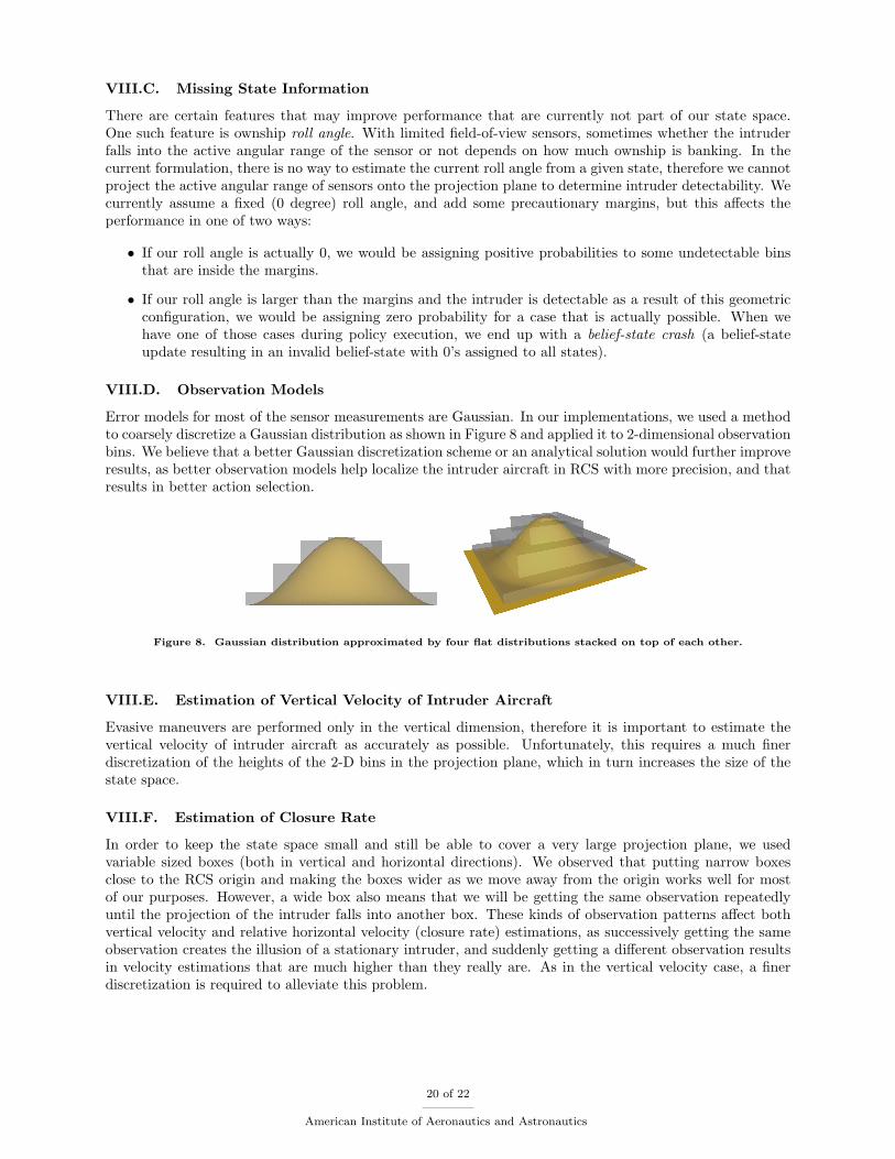
Error models for most of the sensor measurements are Gaussian. In our implementations, we used a methodto coarsely discretize a Gaussian distribution as shown in Figure 8 and applied it to 2-dimensional observationbins. We believe that a better Gaussian discretization scheme or an analytical solution would further improveresults, as better observation models help localize the intruder aircraft in RCS with more precision, and thatresults in better action selection.

Figure 8. Gaussian distribution approximated by four flat distributions stacked on top of each other.

VIII.E. Estimation of Vertical Velocity of Intruder Aircraft

Evasive maneuvers are performed only in the vertical dimension, therefore it is important to estimate thevertical velocity of intruder aircraft as accurately as possible. Unfortunately, this requires a much finerdiscretization of the heights of the 2-D bins in the projection plane, which in turn increases the size of thestate space.

VIII.F. Estimation of Closure Rate

In order to keep the state space small and still be able to cover a very large projection plane, we usedvariable sized boxes (both in vertical and horizontal directions). We observed that putting narrow boxesclose to the RCS origin and making the boxes wider as we move away from the origin works well for mostof our purposes. However, a wide box also means that we will be getting the same observation repeatedlyuntil the projection of the intruder falls into another box. These kinds of observation patterns affect bothvertical velocity and relative horizontal velocity (closure rate) estimations, as successively getting the sameobservation creates the illusion of a stationary intruder, and suddenly getting a different observation resultsin velocity estimations that are much higher than they really are. As in the vertical velocity case, a finerdiscretization is required to alleviate this problem.

20 of 22


IX. Conclusions

This paper has shown that the MDP/POMDP formulation is flexible enough to accommodate a varietyof sensor modalities, intruder behavior, aircraft dynamics, and cost functions. Complex policies produced byMDP/POMDP solvers can be implemented in real time. Both state estimation and policy execution are quiteefficient for the state spaces considered. Current state-of-the-art solvers, using a simplified representationof the aircraft dynamics, can generate useful collision avoidance behavior. Improvements to the problemformulation may further improve performance. In particular, we have limited our formulation to representingmotions in two (relative) dimensions. Moving to full three-dimensional motion in a discretized formulationwill take the size of the state space beyond the range of existing solvers. We need to investigate otherrepresentations for the state space and new types of solvers.

Acknowledgments

The authors wish to thank Nikhil Khanna for his contributions to the early stages of this work while hewas an undergraduate at MIT. Special thanks are due to Dan Griffith, an associate staff member at LincolnLaboratory, who has been tremendously helpful in integrating the MDP collision avoidance system into thesimulation framework.

References

1Abdul-Baki, B., Baldwin, J., and Rudel, M.-P., “Independent Validation and Verification of the TCAS II CollisionAvoidance Subsystem,” AIAA 18th Annual Digital Avionics Systems Conference, 1999.

2Kaelbling, L. P., Littman, M. L., and Cassandra, A. R., “Planning and Acting in Partially Observable StochasticDomains,” Artificial Intelligence, Vol. 101, 1998, pp. 99–134.

3Simmons, R. and Koenig, S., “Probabilistic Robot Navigation in Partially Observable Environments,” Proceedings of theInternational Joint Conference on Artificial Intelligence, 1995, pp. 1080–1087.

4Bandera, C., Vico, F. J., Bravo, J. M., Harmon, M. E., and Iii, L. C. B., “Residual Q-Learning Applied to VisualAttention,” 13th International Conference on Machine Learning, 1996, pp. 20–27.

5Darrell, T. and Pentland, A., “Active Gesture Recognition using Partially Observable Markov Decision Processes,”ICPR96 , 1996, pp. 984–988.

6Roy, N., Pineau, J., and Thrun, S., “Spoken Dialogue Management Using Probabilistic Reasoning,” Proceedings of the38th Annual Meeting of the Association for Computational Linguistics (ACL2000), Hong Kong, 2000.

7Horvitz, E. and Paek, T., “DeepListener: Harnessing Expected Utility to Guide Clarification Dialog in Spoken LanguageSystems,” Proceedings of the Sixth International Conference on Spoken Language Processing (ICSLP 2000), Vol. 1, Beijing,China, October 2000, pp. 226–229.

8Bagnell, J. A. and Schneider, J. C., “Autonomous Helicopter Control using Reinforcement Learning Policy Search Meth-ods,” International Conference on Robotics and Automation, IEEE Press, 2001, pp. 1615–1620.

9Ng, A. Y., Kim, H. J., Jordan, M. I., and Sastry, S., “Autonomous Helicopter Flight via Reinforcement Learning,” NIPS ,2003.

10Pineau, J. and Thrun, S., “High-level robot behavior control using POMDPs,” AAAI Workshop notes, 2002.11Puterman, M. L., Markov Decision Processes: Discrete Stochastic Dynamic Programming, John Wiley & Sons, Inc.,

New York, NY, USA, 1994.12Thiebaux, S., Cordier, M.-O., Jehl, O., and Krivine, J.-P., “Supply Restoration in Power Distribution Systems - A

Case Study in Integrating Model-Based Diagnosis and Repair Planning,” Proceedings of the Twelfth Annual Conference onUncertainty in Artificial Intelligence (UAI-96), 1996, pp. 525–532.

13Hauskrecht, M., Planning and Control in Stochastic Domains with Imperfect Information, Ph.D. thesis, MassachusettsInstitute of Technology, Cambridge, MA, 1997.

14Boutilier, C., “A POMDP formulation of preference elicitation problems,” Eighteenth National Conference on Artificialintelligence, American Association for Artificial Intelligence, Menlo Park, CA, USA, 2002, pp. 239–246.

15Cassandra, A., “A Survey of POMDP Applications,” 1998, Presented at the AAAI Fall Symposium.16Pineau, J., Gordon, G., and Thrun, S., “Point-based value iteration: An anytime algorithm for POMDPs,” International

Joint Conference on Artificial Intelligence (IJCAI), August 2003, pp. 1025–1032.17Smith, T. and Simmons, R. G., “Point-Based POMDP Algorithms: Improved Analysis and Implementation,” Proc. Int.

Conf. on Uncertainty in Artificial Intelligence (UAI), 2005.18Kurniawati, H., Hsu, D., and Lee, W., “SARSOP: Efficient point-based POMDP planning by approximating optimally

reachable belief spaces,” Proc. Robotics: Science and Systems, 2008.19Hsu, D., Lee, W., and Rong, N., “A point-based POMDP planner for target tracking,” Proc. IEEE Int. Conf. on Robotics

& Automation, 2008, pp. 2644–2650.20Hsu, D., Lee, W., and Rong, N., “What makes some POMDP problems easy to approximate?” Advances in Neural

Information Processing Systems (NIPS), 2007.21RTCA, Inc., “Minimum Operational Performance Standards for Traffic Alert and Collision Avoidance System II (TCAS

II) Airborne Equipment,” Tech. Rep. RTCA/DO-185A, SC-147, Washington, DC, December 1997.

21 of 22


22RTCA, “Safety Analysis of Proposed Change to TCAS RA Reversal Logic, DO-298,” RTCA, Inc., Washington, D.C.,Nov. 2005.

23Billingsley, T., Safety Analysis of TCAS on Global Hawk using Airspace Encounter Models, Master’s thesis, Mas-sachusetts Institute of Technology, 2006.

24Kochenderfer, M. J., Espindle, L. P., Kuchar, J. K., and Griffith, J. D., “Correlated Encounter Model for CooperativeAircraft in the National Airspace System,” Project Report ATC-344, 2008.

25Lebron, J. E., Zeitlin, A. D., Spencer, N. A., Andrews, J. W., and Harman, W. H., “System Safety Study of MinimumTCAS II (Traffic Alert and Collision Avoidance System),” Tech. Rep. MTR-83W241, MITRE, Dec. 1983.

26Drumm, A., “Lincoln Laboratory evaluation of TCAS II Logic Version 6.04a,” Project Report ATC-240, 1996.27McLaughlin, M. P., “Safety study of the Traffic Alert and Collision Avoidance System (TCAS II),” Tech. Rep. MTR

97W32, MITRE Corporation, June 1997.28Chludzinski, B., “Lincoln Laboratory evaluation of TCAS II logic version 7,” Project Report ATC-268, 1999.29Russell, S. J. and Norvig, P., Artificial Intelligence: A Modern Approach (Second Edition), Prentice Hall, 2003.30Kuchar, J. K., A Unified Methodology for the Evaluation of Hazard Alerting Systems, Ph.D. thesis, Massachusetts

Institute of Technology, Cambridge, Massachusetts, USA, January 1995.31Kuchar, J. K., “Methodology for Alerting-System Performance Evaluation,” Journal of Guidance, Control, and Dynam-

ics, Vol. 19, No. 2, 1996, pp. 438–444.32Winder, L. F. and Kuchar, J. K., “Evaluation of Collision Avoidance Maneuvers for Parallel Approach,” Journal of

Guidance, Control, and Dynamics, Vol. 22, No. 6, 1999, pp. 801–807.33Tsang, S. M., “Method and Apparatus for Performing Three-Dimensional Alpha/Beta Tracking,” U.S. Patent No.

6,236,899 B1, Filed August 18, 1998, and issued May 22, 2001.34Gray, R. L., “Method of Kalman Filtering for Estimating the Position and Velocity of a Tracked Object,” U.S. Patent

No. 5,051,751, Filed February 12, 1991, and issued September 24, 1991.35Littman, M. L., Cassandra, A. R., and Kaelbling, L. P., “Learning Policies for Partially Observable Environments: Scaling

Up,” ICML, 1995, pp. 362–370.36Mazor, E., Averbuch, A., Bar-Shalom, Y., and Dayan, J., “Interacting Multiple Model Methods in Target Tracking: A

Survey,” IEEE Transactions on Aerospace Electronic Systems, Vol. 34, January 1998, pp. 103–123.37Tanizaki, H., Nonlinear Filters: Estimation and Applications, Springer-Verlag, second (revised and enlarged) ed., 1996.38International Civil Aviation Organization, “Surveillance, radar and collision avoidance,” International Standards and

Recommended Practices, Vol. IV, annex 10, 4th ed., July 2007.

22 of 22


Collision Avoidance for Unmanned Aircraft using Markov Decision...

Documents

Transcript of Collision Avoidance for Unmanned Aircraft using Markov Decision...