IZA DP No. 1506

Collective Female Labour Supply:Theory and Application

Olivier Donni

DI

SC

US

SI

ON

P

AP

ER

S

ER

IE

S

Forschungsinstitut

zur Zukunft der Arbeit

Institute for the Study

of Labor

March 2005

Collective Female Labour Supply:

Theory and Application

Olivier Donni University of Cergy-Pontoise, THEMA,

CIRPEE and IZA Bonn

Discussion Paper No. 1506 March 2005

IZA

P.O. Box 7240 53072 Bonn

Germany

Phone: +49-228-3894-0 Fax: +49-228-3894-180

Email: iza@iza.org

Any opinions expressed here are those of the author(s) and not those of the institute. Research disseminated by IZA may include views on policy, but the institute itself takes no institutional policy positions. The Institute for the Study of Labor (IZA) in Bonn is a local and virtual international research center and a place of communication between science, politics and business. IZA is an independent nonprofit company supported by Deutsche Post World Net. The center is associated with the University of Bonn and offers a stimulating research environment through its research networks, research support, and visitors and doctoral programs. IZA engages in (i) original and internationally competitive research in all fields of labor economics, (ii) development of policy concepts, and (iii) dissemination of research results and concepts to the interested public. IZA Discussion Papers often represent preliminary work and are circulated to encourage discussion. Citation of such a paper should account for its provisional character. A revised version may be available directly from the author.

IZA Discussion Paper No. 1506 March 2005

ABSTRACT

Collective Female Labour Supply: Theory and Application∗

In this paper, we deal with female labour supply in the collective framework. We study married couples and start from the empirical observation that the husband’s labour supply is generally fixed at full-time. We then show that, in this case, structural elements of the decision process, such as individual preferences or the rule that determines the intra-household distribution of welfare, can be identified if household demand for at least one commodity, together with the wife’s labour supply, is observed. These theoretical considerations are followed by an empirical application using French data. JEL Classification: D12, J22 Keywords: collective decisions, female labour supply, commodity demands Olivier Donni Département des sciences économiques École des sciences de la gestion Université du Québec à Montréal Case Postale 8888 Succursale Centre-Ville Montréal (Qc) H3C 3P8 Canada Email: donni.olivier@uqam.ca

∗ Financial support from the Fonds Québecois de Recherche sur la Société et la Culture is gratefully acknowledged. This paper was partly written when I was working at the Université Laval, whose hospitality is gratefully acknowledged. Preliminary versions have been presented in Paris, Lille, Québec and Montréal. We thank François Bourguignon, Pierre-André Chiappori, Bernard Fortin, François Gardes, Guy Lacroix, Thierry Magnac and Costas Meghir for useful comments and suggestions. We also thank Bénédicte Sabatier for her research assistance in the data processing. We bear the sole responsibility for any remaining errors.

1 Introduction

Traditionally, the household, as a whole, is considered the elementary decisionunit; in particular, consumption and labour supply decisions are modelled asthough household members were maximizing a unique utility function undera budget constraint. Nevertheless, this so-called �unitary�approach has beencriticized because, as is generally admitted, a household comprising severaladult members does not necessarily behave as a single rational agent.1

Still another approach is proposed by Chiappori (1988, 1992). This au-thor develops a model of labour supply based on a �collective�representationof household behaviour. In this framework, each person is characterized byspeci�c preferences, and decisions are assumed to result in Pareto-e¢ cientoutcomes. Then, if consumption is purely private and agents are egoistic,e¢ ciency has two attractive properties. First, household labour supply func-tions have to satisfy testable restrictions. Second, if these restrictions aresatis�ed, some elements of the decision process, such as preferences and therule that determines the intra-household distribution of welfare, can be re-trieved from the observation of the labour supply functions. Moreover, Donni(2003) shows that this theoretical model can be extended to incorporate thepossibility of non-participation decisions and nonlinear budget sets.2

The collective approach turns out to be pro�table, as shown by recentempirical applications. For example, Fortin and Lacroix (1997) closely fol-low Chiappori�s initial framework and �nd, using Canadian data, that therestrictions implied by the collective setting are not rejected. Chiappori etalii (2002) extend this framework to allow for �distribution factors�, de�nedas being any variable that is exogenous with respect to preferences but mayin�uence the decision process. Using the PSID and choosing the sex ratioand an indicator of divorce legislation as distribution factors, they also �ndthat the theoretical restrictions are not rejected.Unfortunately, these empirical investigations do not account for the fact

that, in the majority of developed countries, male labour supply is rigid andlargely determined by exogenous constraints. This is a serious problem thatwas recently addressed by Blundell et alii (2001). These authors examine

1In addition, the speci�c restrictions imposed by the unitary model have received littleempirical support, if any. See Lundberg and Pollak (1996) on this point.

2Fong and Zhang (2001) study a collective model of labour supply where there are twodistinct types of leisure: one type of leisure can be seen as �private�and the other type as�public�. See Vermeulen (2002) for a survey of collective models.

2

United Kingdom data from 1978 to 1993 and remark that, when men work,they nearly always work full-time, while wive�s hours of work, on the contrary,vary widely. The theoretical model they develop allows for these essentialfeatures: the wife�s labour supply is assumed to be continuous whereas thehusband�s choices are assumed to be discrete (either working full time or notat all). They show that the main conclusions, derived by Chiappori in theinitial context, are still valid here. One drawback, however, is that such adi¤erence in spouses�behaviour is completely unexplained. Moreover, theresult of identi�ability and testability given by Blundell et alii (2001) holdsonly if the husband�s choice between working full time and not working isfree. In particular, it could be seriously misleading if the husband�s unem-ployment, which is due to demand-side constraints, is mistakenly interpretedin empirical studies as a decision to not participate in the labour market. Asa matter of fact, the model of Blundell et alii (2001) is probably convenientwhen the labour market is very competitive since, in this case, a large pro-portion of non-working men can be explained by free decisions. Nonetheless,the pertinence of this model to the study of female labour supply is certainlymore questionable when the labour market is very regulated.Our objective in this paper is to investigate female labour supply in

France, where a high proportion of unemployment in the population canbe seen, in all likelihood, as involuntary.3 To do that, we have to handle therigidity of the husband�s behaviour in a quite di¤erent way. Our startingpoint follows Blundell et alii (2001), though. We admit the empirical factthat, for the majority of households, the husband�s hours of work are �xedat full-time while the wife�s hours of work are spread between zero and thefull-time bound. This is at least a good approximation. Now, our approachdi¤ers from Blundell et alii (2001), in that the few husbands who do not workare seen as being constrained by involuntary unemployment. In that case,the large proportion of husbands who work full-time can simply be explainedby their preferences between leisure and consumption. The crucial point,then, is that the husband�s hours of work, if they do not vary or if they aredetermined by demand-side constraints, tell us nothing about the decisionprocess or preferences. Consequently, the results given by Chiappori (1988,1992) or Blundell et alii (2001) are no longer valid in the present context.

3See Laroque and Salanié (2002) for a recent investigation of the role of the minimumwage, together with welfare bene�ts, in explaining unemployment in France. They stressthat the actual cost of the minimum wage to the employer is particularly high in France.

3

To deal with that, we adopt an alternative approach that is inspired by theliterature on collective models of consumption4 and, to simplify matters, weignore the case of households with unemployed husbands. That is to say, ourtheoretical model focusses on households with husbands working full time�the most common situation� and considers the observation of wive�s laboursupply, together with information given by the structure of household con-sumption, to identify the most important elements of the decision processand understand how wive�s hours of work are determined.The next steps are then as follows. First, we extend to collective mod-

els the theory of household behaviour under rationing, previously developedby Neary and Roberts (1980) for the unitary approach. This is necessaryfor studying household behaviour when the labour supply of one spouse is�xed at zero or full-time. Second, assuming that the husband�s labour sup-ply is �xed, we demonstrate that the main properties of Chiappori�s initialmodel are preserved. In particular, some elements of the intra-householddecision process can be identi�ed from the observation of the wife�s laboursupply function and on one commodity demand function.5 Third, using atechnique based on Blundell et alii (2001) and Donni (2003), we prove thatthis model is still identi�able and testable if the wife does not work. Thistheoretical advance is empirically relevant since it is generally observed thata large number of women do not participate in the labour market. The �nalcontribution of this paper is to estimate and test this model using Frenchdata for couples in which only the husband is working full-time. In this em-pirical exploration, we take into account the possibility of non-participationof the wife and estimate a �ve-equation system (one labour supply and fourcommodity demands).This paper is structured as follows. Section 2 discusses the assumptions

of our framework and Section 3 presents the main theoretical results. Section4 provides an analysis of our econometric strategy and Section 5 gives a briefdescription of the data and the empirical results. Section 6 concludes.

4The main result of this literature is that the intra-household distribution of resourcescan be retrieved from the observation of a system of commodity demand functions. SeeBourguignon et alii (1995) and Chiappori and Ekeland (2002a, 2002b) for the theory, andBrowning et alii (1994) and Browning and Chiappori (1998) for empirical applications.

5A related result was already mentioned in Bourguignon et alii (1995) in the contextof demand analysis with constant prices. The identi�cation result that we present inthis paper is more general, however, since the price of the wife�s leisure is assumed to bevariable.

4

2 The Collective Approach

2.1 General Framework

We consider only the case of married couples (m and f) in a single periodsetting.6 The wife�s and husband�s labour supply are respectively denoted byLf and Lm with market wages wf and wm. The wife�s and husband�s demandfor commodity n (n = 1; : : : ; N , with N > 2) are respectively denoted byQfn and Qmn with prices set to one. Non-labour income is denoted by y.For convenience, each spouse�s total time endowment is normalized at one7

and we say that member i (i = m; f) works full-time if Li = 1. Let Qi =(Qi1; : : : ; QiN) be the vector of member i�s consumptions. We adopt thefollowing assumption on preferences.

Assumption A1 Each household member is characterized by speci�c pref-erences. These can be represented by utility functions of the form: ui(1 �Li;Qi) that are both strongly concave, in�nitely di¤erentiable and strictlyincreasing in all their arguments, with limQin!0 u

i(1� Li;Qi) = �1.The household members are said to be �egoistic�in the sense that their

utility only depends on their own consumption and leisure. However, allthe results immediately extend to the case of �caring�agents, with utilitiesrepresented by the form:

Wi[um(1� Lm;Qm); uf (1� Lf ;Qf )],

where Wi(�) is a strictly increasing function; see Chiappori (1992) on thispoint. Finally, let us note that the condition on limits in A1 lets us rule outcases in which individual consumption is equal to zero.We implicitly assume that there is no public consumption and no domestic

production. The budget set is then written as follows:

y + Lfwf + Lmwm >

PNn=1(Q

fn +Qmn); (1)

1 > Li > 0 and Qin > 0 (n = 1; : : : ; N and i = f;m) . (2)

6Of course, the fact that the household members are married is not important. Theterminology is just for convenience.

7This upper bound for hours of work can alternatively be seen as a legal or socio-culturalnorm. At this stage, we do not favour any particular interpretation.

5

We observe that, in surveys, consumption is generally recorded at the house-hold level. We thus assume, in what follows, that only the vector of aggregateconsumptions, Q = Qf +Qm, is observed by the econometrician.The main originality of the e¢ ciency approach lies in the fact that house-

hold decisions result in Pareto-e¢ cient outcomes and that no additional as-sumptions are made about the process. This is formally expressed in thefollowing assumption.

Assumption A2 The outcome of the decision process is Pareto e¢ cient;that is, for any wage-income bundle (wf ; wm; y), the labour-consumption bun-dle (Lf ; Lm;Qf ;Qm) chosen by the household is such that no other bundle(�Lf ; �Lm; �Qf ; �Qm) in the budget set could make both members better o¤.

This assumption has a good deal of intuitive appeal. The household isone of the preeminent examples of a repeated game. Thus, given symmetryof information, it is plausible that agents �nd mechanisms to support e¢ -cient outcomes since cooperation often emerges as a long-term equilibriumof repeated noncooperative relations.In this theoretical discussion, we suppose that there is no involuntary

unemployment. Then, Pareto-e¢ ciency essentially means that there existsa scalar � such that household behaviour can be described as a solution tofollowing program:

maxfLf ;Lm;Qf ;Qmg

(1� �) � uf (1� Lf ;Qf ) + � � um(1� Lm;Qm) (P)

with respect to budget sets (1) and (2). The parameter � has an obviousinterpretation as a �distribution of power�index. If � = 0, then the householdbehaves as though the wife always gets her way, whereas if � = 1; the husbandis the e¤ective dictator. Moreover, to obtain well-behaved labour supply andcommodity demand functions, we assume that the scalar � 2]0; 1[ is a single-valued and in�nitely di¤erentiable function of wf , wm and y. The underlyingidea is that, within a bargaining context, the threat point is expected todepend on non-labour income and the wage that the spouses receive whenthey work.

2.2 Decentralization and Rationing

To begin with, we say that a pair of labour supply functions, Lf (wf ; wm; y)and Lm(wf ; wm; y), together with a pair of systems of commodity demand

6

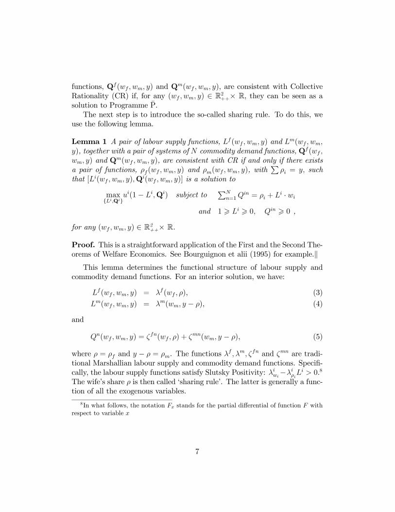
functions, Qf (wf ; wm; y) and Qm(wf ; wm; y), are consistent with CollectiveRationality (CR) if, for any (wf ; wm; y) 2 R2++� R, they can be seen as asolution to Programme P.The next step is to introduce the so-called sharing rule. To do this, we

use the following lemma.

Lemma 1 A pair of labour supply functions, Lf (wf ; wm; y) and Lm(wf ; wm;y), together with a pair of systems of N commodity demand functions, Qf (wf ;wm; y) and Qm(wf ; wm; y), are consistent with CR if and only if there existsa pair of functions, �f (wf ; wm; y) and �m(wf ; wm; y), with

P�i = y; such

that [Li(wf ; wm; y);Qi(wf ; wm; y)] is a solution to

maxfLi;Qig

ui(1� Li;Qi) subject toPN

n=1Qin = �i + L

i � wi

and 1 > Li > 0; Qin > 0 ,

for any (wf ; wm; y) 2 R2++� R.

Proof. This is a straightforward application of the First and the Second The-orems of Welfare Economics. See Bourguignon et alii (1995) for example.kThis lemma determines the functional structure of labour supply and

commodity demand functions. For an interior solution, we have:

Lf (wf ; wm; y) = �f (wf ; �), (3)

Lm(wf ; wm; y) = �m(wm; y � �), (4)

and

Qn(wf ; wm; y) = �fn(wf ; �) + �

mn(wm; y � �), (5)

where � = �f and y � � = �m. The functions �f ; �m; �fn and �mn are tradi-tional Marshallian labour supply and commodity demand functions. Speci�-cally, the labour supply functions satisfy Slutsky Positivity: �iwi��

i�iLi > 0.8

The wife�s share � is then called �sharing rule�. The latter is generally a func-tion of all the exogenous variables.

8In what follows, the notation Fx stands for the partial di¤erential of function F withrespect to variable x

7

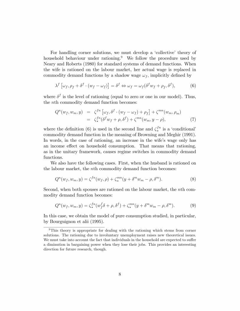
For handling corner solutions, we must develop a �collective� theory ofhousehold behaviour under rationing.9 We follow the procedure used byNeary and Roberts (1980) for standard systems of demand functions. Whenthe wife is rationed on the labour market, her actual wage is replaced incommodity demand functions by a shadow wage !f ; implicitly de�ned by

�f�!f ; �f + �

f � (wf � !f )�= �f , !f = !f (�

fwf + �f ; �f ), (6)

where �f is the level of rationing (equal to zero or one in our model). Thus,the nth commodity demand function becomes:

Qn(wf ; wm; y) = �fn�!f ; �

f � (wf � !f ) + �f�+ �mn(wm; �m)

= �fn? (�fwf + �; �

f ) + �mn(wm; y � �), (7)

where the de�nition (6) is used in the second line and �fn? is a �conditional�commodity demand function in the meaning of Browning and Meghir (1991).In words, in the case of rationing, an increase in the wife�s wage only hasan income e¤ect on household consumption. That means that rationing,as in the unitary framework, causes regime switches in commodity demandfunctions.We also have the following cases. First, when the husband is rationed on

the labour market, the nth commodity demand function becomes:

Qn(wf ; wm; y) = �fn(wf ; �) + �

mn? (y + �mwm � �; �m): (8)

Second, when both spouses are rationed on the labour market, the nth com-modity demand function becomes:

Qn(wf ; wm; y) = �fn? (w

ff � + �; �

f ) + �mn? (y + �mwm � �; �m): (9)

In this case, we obtain the model of pure consumption studied, in particular,by Bourguignon et alii (1995).

9This theory is appropriate for dealing with the rationing which stems from cornersolutions. The rationing due to involuntary unemployment raises new theoretical issues.We must take into account the fact that individuals in the household are expected to su¤era diminution in bargaining power when they lose their jobs. This provides an interestingdirection for future research, though.

8

3 Collective Female Labour Supply

3.1 Preliminary Considerations

In the collective model of labour supply, initially developed by Chiappori(1988, 1992), the solutions to Programme P are assumed to be interior.Speci�cally, it is implicitly assumed that (wf ; wm; y) 2 R; where R is de-�ned by

R ��(wf ; wm; y) 2 R2++ � R

�� 1 > Li(wf ; wm; y) > 0; i = f;m :Such a framework, where labour supplies are characterized by (3) and (4),allows us to recover preferences and the outcome of the decision process fromthe observation of labour supply functions.In some countries, however, the assumption that both labour supplies

freely vary is not appropriate. We often observe, as indicated in the in-troduction, that the husband�s labour supply is �xed at the current upperbound (i.e., Lm = 1) for the majority of households and equal to zero fora minority of them. Our framework is hardly consistent with this empiricalfact, unless we assume that the husband�s unemployment we observe is dueto demand-side constraints. This is the idea underlying our approach. Wenow proceed as follows. First of all, in keeping with the previous section,we focus on the behaviour of households which are not a¤ected by unem-ployment. Then, we admit that, for unknown reasons, the husband has littletaste for leisure and/or is able to obtain a high market wage. This implies,in our setting, that he always chooses the maximum number of hours at hisdisposal. Formally, assume that (wf ; wm; y) 2 P; where P is de�ned by

P ��(wf ; wm; y) 2 R2++ � R

�� 1 > Lf (wf ; wm; y) > 0; Lm(wf ; wm; y) = 1 :In other words, the theoretical model that follows analyses the householdmembers�desired hours of work, between zero and one, but supposes thatthe husband always chooses the maximum number of hours available.10

One noteworthy point is that, if (wf ; wm; y) 2 P , the observation of thesole labour supply functions does not allow us to test e¢ ciency or identify

10This maximum is assumed the same for all workers. Of course, this line of argumentis valid only if �overtime�hours are not possible.

9

useful structural elements of the model.11 In fact, the observation of the hus-band�s labour supply function does not contain useful information. The ideaof this paper is then to use the observation of the structure of consumptionto identify the sharing rule and derive testable restrictions.

3.2 Identifying the Sharing Rule

First, we assume that only one commodity demand function, together withthe wife�s labour supply function, is observed. We recall that when thehusband�s labour supply is �xed at one, these functions are written as:

Lf (wf ; wm; y) = �f (wf ; �),

Qn(wf ; wm; y) = �fn(wf ; �) + �mn? (y + wm � �; 1),

where the sum of non-labour income and the husband�s wage is the �exoge-nous� household income. Moreover, under our assumptions, Lf (wf ; wm; y)and Qn(wf ; wm; y) as well as �(wf ; wm; y) are in�nitely di¤erentiable in alltheir arguments on int(P ). To simplify derivation of the results, we nowintroduce the following de�nitions:

�n =QnyL

fwm � LfyQnwmLfwm � Lfy

and �n =Lfwm � Lfy

�nyLfwm � �nwmL

fy

,12

if Lfwm 6= Lfy and �nyL

fwm 6= �nwmL

fy : We also assume that the functions we

consider satisfy the following regularity conditions.

Assumption R1 The wife�s labour supply function and the nth commod-ity demand function are such thatLfwm 6= Lfy , �nwm 6= �ny and �nyLfwm 6= �nwmLfyfor any (wf ; wm; y) 2 int(P ).The �rst condition obviously implies the absence of income pooling in

the wife�s labour supply, i.e., the impact of the husband�s wage and of non-labour income on the wife�s labour supply are di¤erent. The other conditionsare more complicated and not examined here. Quite importantly, however,

11On the contrary, in the unitary approach, we have testable constraints on the wife�slabour supply function even if the husband�s labour supply does not vary (e.g., IncomePooling and Slutsky Positivity). Furthermore, �household�preferences between the wife�sleisure and consumption can then be identi�ed from observation of the wife�s labour supply.

10

it can be shown that these conditions exclude the demand function for the�composite�commodity Z (say) which is de�ned by Z =

PNn=1(Q

fn +Qmn).We can now put forward the next result, which says that some elements

of the wife�s preferences and the sharing rule can be retrieved.

Proposition 2 Let us assume CR. The functions Lf (wf ; wm; y) and Qn(wf ;wm; y) are observed. Then, under R1, the sharing rule can be retrieved on Pup to a constant �. Speci�cally, its derivatives on int(P ) are given by

�wf = ��nwf�n, �wm = 1� �

nwm�

n and �y = 1� �ny�n:

Moreover, for each choice of �, the wife�s preferences between total consump-tion and leisure are uniquely de�ned. Finally, the individual nth commoditydemand function can also be recovered up to a constant �n.

Proof. See the Appendix.kWe brie�y sketch the basic steps of the proof. The idea is that changes

in either non-labour income or the husband�s wage can only a¤ect the wife�slabour supply insofar as her share of exogenous income, as de�ned by thesharing rule, is modi�ed. This means that any simultaneous change in non-labour income and the husband�s wage that leaves the wife�s labour supplyunchanged must keep her share constant as well. From this idea, it is possibleto measure the e¤ect of exogenous income on commodity demand, keepingthe wife�s share unchanged. This yields the husband�s Engel curve, which inturn allows us to derive other structural elements, like the sharing rule, bydi¤erentiation of the Engel curve and resolution of the resulting system ofpartial di¤erential equations.

3.3 Testing Collective Rationality

The next result gives a set of testable restrictions that the wife�s laboursupply function and the nth commodity demand function must satisfy.

Proposition 3 Let us assume CR. The functions Lf (wf ; wm; y) and Qn(wf ;wm; y) are observed. Then, under R1,

1) Lfwf �Lfwm � Lfy

(�nwm � �ny ) � �n

�Lf � �nwf � �

n�> 0;

2) �nwf�nwm = �

nwm�

nwf

and �nwf�ny = �

ny�

nwf,

for any (wf ; wm; y) 2 int(P ).

11

Proof. See the Appendix.kThese restrictions provide a joint test of collective rationality under spe-

ci�c assumptions, namely, egoistic (or caring) agents and the absence of pub-lic consumption and domestic production. The �rst condition corresponds toSlutsky Positivity translated in the collective approach. The second con-dition results from the separability property of the behavioural functions:the husband�s wage and non-labour income a¤ect household behaviour onlythrough the individual shares.More can be obtained when the demand for several commodities, rather

than a single one, is observed. This is formally expressed in the followingproposition.

Proposition 4 Let us assume CR. The functions Lf (wf ; wm; y), Qn1(wf ;wm; y) and Qn2(wf ; wm; y) are observed. Then, under R1,

�n1wf � �n2wm = �

n2wf� �n1wm and �n1wf � �

n2y = �n2wf � �

n1y ,

for any (wf ; wm; y) 2 int(P ).

Proof. See the Appendix.kThe di¤erence with the case of only one commodity is that the constraints

here are based on a second, rather than a third order partial di¤erentialequation, which is more restrictive.

3.4 Extension: The Wife�s Rationing

One of the main limitations of the preceding results is the assumption thatthe wife is always free to vary the hours she works. Indeed, many wiveschoose not to work at all or to work full-time, two cases ruled out in theearlier discussion. In this section, we thus consider the wife�s participationdecision. The results can easily be extended to the converse case of workingfull-time, though.First, we note that the existence of a well-behaved participation frontier

does not stem from the theoretical construct as in standard labour supply

12

models, but must be postulated.13 Therefore, we use the following assump-tion.

Assumption R2 There exists a positive function (wm; y) de�ned on R++� R such that the wife does not participate in the labour market if and onlyif wf 6 (wm; y).We also assume that the wife�s market wage wf is observed even when

she does not work. Of course, this is very restrictive but, in practice, themarket wage can be estimated by an auxiliary equation.14 We thus supposethat (wf ; wm; y) 2 N where N is de�ned by

N ��(wf ; wm; y) 2 R2++ � R

�� Lf (wf ; wm; y) = 0, Lm(wf ; wm; y) = 1 .We also de�ne I � f(wm; y)j(wf ; wm; y) 2 N and wf = (wm; y)g. In Figure1, the sets P , N and I are illustrated in a two-dimensional plane (i.e., for a�xed y). We see, in this �gure, that the wife does not work when her wage isbelow its reservation value (given by the curve in bold) and she works full-time when her wage is above some critical value (given by the upper curve).15

We can say the same for the husband.We �nally assume that we observe the nth commodity demand function,

given by

Qn(wf ; wm; y) = �fn? (�; 0) + �

mn? (y + wm � �; 1)

and the participation frontier, de�ned as wf = (wm; y). Under our assump-tions, this commodity demand function and the participation frontier arein�nitely di¤erentiable on int(N) and I, respectively. Moreover, along theparticipation frontier, the nth commodity demand function can be writtenas follows:

Qn(wm; y) = Qn [ (wm; y); wm; y] .

13The idea is that, when the wife is indi¤erent between working and not working, asmall increase in her wage has a substitution e¤ect� as in the standard model� but alsoan income e¤ect through the sharing rule. The former is necessarily positive but the lattercan be positive or negative. See Blundell et alii (2001) and Donni (2003) for a formaldiscussion.14Still, the treatment of this issue may raise very complicated problems which are not

addressed here. See Blundell et alii (2001) for a �rst investigation.15The wife�s (husband�s) labour supply, if it is backward bending, may fall below 1 for

some wages which are particularly high, but this feature is not represented in Figure 1.

13

wf = γ(wm, y*)

wf

wm

Lm = 00 < Lf <1

Lm = 0Lf = 0

0 < Lm < 10 < Lf < 1 P

0 < Lm < 1Lf = 0 N

Lm = 0Lf = 1

0 < Lm < 1Lf = 1

Lm = 1Lf = 1

I

Figure 1: A Two-dimensional Illustration of Rationing Sets (with y = con-stant)

The latter is in�nitely di¤erentiable on I. The next step is to de�ne thefollowing functions:

An =Qny wm � yQnwm

wm � yand Bn =

wm � y wmA

ny � yAnwm

,

if wm 6= y and wmAny 6= yA

nwm, and introduce the following regularity

condition.

Assumption R3 The wife�s participation frontier and the nth commoditydemand are such that wm 6= y, Anwm 6= Any , wmAny 6= yAnwm and Cnwm 6= Cnyfor any (wm; y) 2 I.The next result says, �rst, that the sharing rule can be retrieved on N

up to a constant and, second, that testable restrictions are generated.

Proposition 5 Let us assume CR. The functions (wm; y) and Qn(wf ; wm;y) are observed. Then, under R2 and R3, the sharing rule can be retrieved on

14

N up to a constant �. Speci�cally, let �(wm; y) = � [ (wm; y); wm; y]. Then,the derivatives of �(wm; y) on I are given by

�wm = 1� AnwmBn and �y = 1� AnyBn:

Moreover, the individual nth commodity demand can be retrieved up to aconstant �n. Finally, we have the following constraint:

AnyBnwm = A

nwmB

ny ,

for any (wm; y) 2 I.

Proof. See the Appendix.

At this stage, some clari�cations are necessary. First, the proof of thisproposition does not require complete speci�cation of the wife�s underlyinglabour supply, but only of the participation frontier. This result is usefulsince surveys generally contain information about the employment status ofhousehold members but not necessarily about the number of hours of work.The wife�s wage must be observed, though. Second, considering additionalcommodity demands obviously creates new constraints. These are not for-mally examined in this paper. In fact, commodity demand functions with�double rationing�receive great attention in Bourguignon et alii (1995). Inparticular, these authors show that a triplet of commodity demand functionsis su¢ cient to identify the sharing rule. By comparison, the result aboverequires only one commodity demand function and the participation fron-tier. Finally, the results of Proposition 5 complete those of Proposition 2and ensure that the sharing rule is identi�ed on the entire set of interest tous, P [N .

4 Econometric Analysis

In this section, we consider empirical implementation of the model describedabove. First, we propose a functional form for labour supply and the systemof commodity demands. Second, we introduce stochastic terms and derivethe log-likelihood function.

15

4.1 Functional Form

In this section and those that follow, we adopt the following conventions : wfhdenotes the wife�s hourly wage in household h, wmh the husband�s hourlywage, yh monthly non-labour income, Lfh the observed number of hoursworked per month, Qnh expenditure on commodity n per month, and T the(legal or socio-cultural) maximum number of hours per month.

4.1.1 Labour Supply and Commodity Demands

In order to estimate and test this model, we adopt the linear functional form,initially proposed by Hausman (1981), for the wife�s latent labour supply. Ifwe ignore the stochastic terms at this stage, we have:

L�fh = �h + �wfh + �h, (10)

where L�fh is the wife�s latent number of worked hours per month. The wifeis rationed on the labour market if the latent variable is either greater thanT or less than 0:

Lfh = T if L�fh > T ,Lfh = 0 if L�fh 6 0,Lfh = L�fh otherwise.

Moreover, the intercept �h is assumed to depend on a set of variables:

�h =PJ

j=1 �j � zjfh,

where zjfh are socio-demographic characteristics relevant for explaining thewife�s behaviour (e.g., the wife�s age, the region of residence, the numberof children). Finally, Slutsky Positivity is globally ful�lled if and only if� > max(0; T ).This speci�cation has several desirable properties. First, the linear form

for labour supply has frequently been used in empirical studies and is suitablefor French data; see Bourguignon and Magnac (1990) for another applica-tion.16 Second, the wife�s preferences between leisure and consumption have

16We tested a more �exible functional form by introducing a second-order polynomialin �h, but the coe¢ cient associated with this term proved to be insigni�cant. Otherspeci�cations (e.g., a logarithmic term for wfh) were also tried unsuccessfully.

16

a well-known form; see Hausman (1981). They are described by the followingindirect utility function:

V (wfh; �h) = exp( wfh) ���h +

�

wfh �

�

2+�h

�: (11)

Third, and more importantly, this speci�cation permits us to have a closedform for shadow wages which are used to compute rationed commodity de-mand functions. Of course, the main limitation of the linear functional formis its lack of �exibility; in particular, it implies, when Slutsky Positivity isimposed, that the labour supply curve is upward sloping everywhere.We now consider the functional form of the commodity demands. We

assume that, when 0 < L�fh < T , the nth commodity demand function isquadratic,17 as follows:

Qnh = anfh + bnfwfh + c

nf�h + d

nf�h

2 + anmh + cnm(yh + wmhT � �h)

+ dnm(yh + wmhT � �h)2:

According to our theory, this functional form switches regimes in the pres-ence of rationing. Two cases must be considered. First, when L�fh 6 0, wecompute a shadow wage as follows:

!fh = ��h + � �h

�,

and introduce this expression into the nth commodity demand to obtain:

Qnh = anfh + bnf!fh + c

nf�h + d

nf�h

2 + anmh + cnm(yh + wmhT � �h)

+ dnm(yh + wmhT � �h)2:

Second, when L�fh > T , the shadow wage becomes :

!fh =T � �h � � (wfhT + �h)

� � T ,

and we introduce this expression into the nth commodity demand. Since thissubstitution also in�uences the shadow income, we obtain:

Qnh = anfh + bnf!fh + c

nf ((wfh � !fh)T + �h) + dnf ((wfh � !fh)T + �h)2

+ anmh + cnm(yh + wmhT � �h) + dnm(yh + wmhT � �h)2:

17Using our data, we also experimented with a functional form with a third-order termin �h and in (y + whT � �h); but these terms turn out to be statistically insigni�cant.

17

This way of dealing with rationing implies that commodity demand functionsare continuous everywhere (in particular, along the frontiers where the regimeswitches) and an increase in the wife�s wage, in the case of rationing, only hasan income e¤ect on consumption. Finally, since individual intercepts cannotbe both identi�ed, we reset the parameters anh = a

nfh + a

nmh with

anh =PJ

j=1 anj � zjh,

where zjh are socio-demographic variables relevant for explaining the spouses�behaviour.

4.1.2 The Sharing Rule and the Collective Constraints

As in Fortin and Lacroix (1997) and Blundell et alii (2001), we adopt a linearspeci�cation for the sharing rule:

�h = A � wfhT +B � wmhT + C � yh. (12)

Although the sign of the parameters is not formally determined by the modelabove, intuition suggests that

0 < B < C < 1:

However, the coe¢ cient A can be either positive or negative since its signresults from two opposite e¤ects; see Chiappori (1992). To show that, let usassume that the wife�s wage rises. If she works, the income of the household,as a whole, should increase and both members should bene�t from that. Atthe same time, however, the wife improves her bargaining power. This laste¤ect should have a negative impact on the husband�s share. All in all, thenegative impact of the wife�s wage on the husband�s share likely predominatesif the welfare gains resulting from the wage increase are small enough (notablyif the wife does not work).18 Speci�cally, if we introduce the sharing rule (12)into the utility function (11), di¤erentiate with respect to wfh; and use (10),we can demonstrate that the wife bene�ts from an increase in her wage onlyif

A+LfhT> 0: (13)

18In principle, these two e¤ects could be modelled by assuming that the sharing ruleswitches regimes in the case of rationing. There is, however, a potential problem of logicalconsistency if the sharing rule is assumed to be a function of the wife�s observed hours ofwork.

18

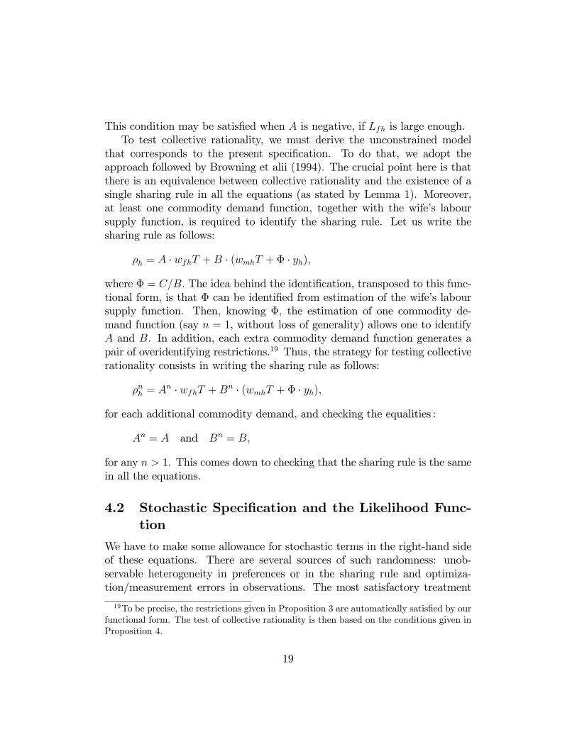
This condition may be satis�ed when A is negative, if Lfh is large enough.To test collective rationality, we must derive the unconstrained model

that corresponds to the present speci�cation. To do that, we adopt theapproach followed by Browning et alii (1994). The crucial point here is thatthere is an equivalence between collective rationality and the existence of asingle sharing rule in all the equations (as stated by Lemma 1). Moreover,at least one commodity demand function, together with the wife�s laboursupply function, is required to identify the sharing rule. Let us write thesharing rule as follows:

�h = A � wfhT +B � (wmhT + � � yh),

where � = C=B: The idea behind the identi�cation, transposed to this func-tional form, is that � can be identi�ed from estimation of the wife�s laboursupply function. Then, knowing �, the estimation of one commodity de-mand function (say n = 1, without loss of generality) allows one to identifyA and B. In addition, each extra commodity demand function generates apair of overidentifying restrictions.19 Thus, the strategy for testing collectiverationality consists in writing the sharing rule as follows:

�nh = An � wfhT +Bn � (wmhT + � � yh),

for each additional commodity demand, and checking the equalities :

An = A and Bn = B,

for any n > 1. This comes down to checking that the sharing rule is the samein all the equations.

4.2 Stochastic Speci�cation and the Likelihood Func-tion

We have to make some allowance for stochastic terms in the right-hand sideof these equations. There are several sources of such randomness: unob-servable heterogeneity in preferences or in the sharing rule and optimiza-tion/measurement errors in observations. The most satisfactory treatment

19To be precise, the restrictions given in Proposition 3 are automatically satis�ed by ourfunctional form. The test of collective rationality is then based on the conditions given inProposition 4.

19

would be to allow for each of these and to develop a full stochastic model (seeBlundell et alii (2001) for such an attempt in a less complicated context).However, this would entail the introduction of a large number of stochasticterms and make the model almost intractable. More importantly, the distri-bution of these terms is not necessarily identi�able. Hence we adopt a muchmore conventional approach of simply adding error terms to each equation:�h for the wife�s labour supply and "nh for the nth commodity demand.We assume that the vector (�h; "1h; : : : ; "

Nh ) follows a multidimensional

normal distribution with mean zero and a covariance matrix given by

� if 0 < L�fh < T ,

�0 = �0 � � � �00 if L�fh 6 0,�1 = �1 � � � �01 if L�fh > T ,

where � is a matrix of free parameters and �0 and �1 are identity matri-ces with free parameters instead of zeros in the �rst column. This speci-�cation is a convenient approximation when stochastic terms in the wife�slabour supply result from a mix of unobservable taste heterogeneity and op-timization/measurement errors (it is a straightforward generalization of theapproach of Kooreman and Kapteyn (1986) to the case of more than twoequations).20 This re�ects the fact that, in the case of rationing, the tasteheterogeneity factor in the wife�s labour supply is �introduced�into commod-ity demands through shadow wages.These assumptions, with the relationships de�ned above, directly yield

a distribution on hours of work and commodity quantities. There are threeregimes. Wives are either unrationed, rationed at 0; or rationed at T . Letus denote Rh = ��h � �wfh � �h; Rh = T � �h � �wfh � �h; and

g : (Lfh; Q1h; : : : ; Q

Nh )! (�h; "

1h; : : : ; "

Nh )

the relationship between observations and stochastic terms. The density forwives who are unrationed is given by

f(Lfh; Q1h; : : : ; Q

Nh ) = ��(�h; "

1h; : : : ; "

Nh )

= ���g(Lfh; Q

1h; : : : ; Q

Nh )�,

where �� denotes the multidimensional normal density with a mean of zeroand a matrix � of covariances (the determinant of the Jacobian matrix for

20The inaccuracy in the distribution of the random terms is the price of our rejection ofa full stochastic speci�cation.

20

the variable transformation is equal to one). Then the contribution to thelikelihood for wives who are rationed at 0 is given by

F0(Q1h; : : : ; Q

Nh ) =

Z Rh

�1��0(�h; "

1h; : : : ; "

Nh ) � d�h

=

Z 0

�1��0

�g(L�fh; Q

1h; : : : ; Q

Nh )�� dL�fh:

Similarly, the contribution for wives who are rationed at T is given by

F1(Q1h; : : : ; Q

Nh ) =

Z +1

Rh

��1(�h; "1h; : : : ; "

Nh ) � d�h

=

Z +1

T

��1�g(L�fh; Q

1h; : : : ; Q

Nh )�� dL�fh:

Finally, combining these expressions provides the log-likelihood function ofthe econometric model:

L(Lfh; Q1h; : : : ; Q

Nh ) =

PLfh=0

lnF0 +P

Lfh=TlnF1 +

P0<Lfh<T

ln f .

A critical assumption in the above analysis concerns the observability of thewage for all wives. This is, of course, not the case for unemployed women.Our approach is thus based on the construction of a �tted value wfh for thewage using censored regression techniques and interprets wfh as the wagefaced by all workers.

5 Data and Empirical Results

In this section we present the main results. First we describe the data set,then we give the estimated coe¢ cients and the statistics for the test of thecollective constraints.

5.1 The Data

Data are drawn from the household survey �Budget des Familles�conductedby the national institute of economic and statistical information of France(INSEE) in a sample of 12,000 French households in 1984�85. The surveycontains detailed information on earnings and income from property andtransfers, on expenditures for nondurable as well as durable commodities, on

21

most socio-demographic characteristics of individuals and households and,�nally, on the number of hours and the work status of individuals. Severalstudies have used this survey over the last 10 years, allowing some interestingcomparisons to be made. For instance, Bourguignon et alii (1993) use asample extracted from this survey to test the collective approach in a contextof pure consumption. They do not reject the theoretical restrictions.From the original sample, we �rst select a subsample of married couples

with, at most, one child between 3 and 18 years old. Children, and ex-penditures on them, may indeed be considered public commodities for bothparents, whereas the model considered above only allows for private com-modities. Moreover, children are expected to increase problems related tohousehold production. On the other hand, considering only childless couplesrestricts the size of our sample considerably.We next restrict the sample to couples in which husband and wife (if they

are working) are not self-employed.21 These selection rules and the exclusionof observations with missing data leave us with a total of 1078 observations.The distribution of working hours in this sample is described in Table 1.However, according to our theory, the sample we use in the empirical analysismust contain only couples that are not a¤ected by involuntary unemploymentand in which the husband works full-time (i.e., arbitrarily de�ned by monthlylabour supply above 140 hours). Hence, we remove 200 extra observationsand obtain a �nal sample of 878 households.22 Conditioning the sampleon full-time working husbands may, in principle, induce a selectivity bias.However, the number of households in which the husband does not workfull-time is small. In addition, it is predominantly made up of job seekers(even if this may hide a voluntary decision) and one may reasonably believethat the problem of selection is less important in this case. In particular, itmay be completely negligible if unemployment indiscriminately strikes anyhousehold regardless of the wife�s and husband�s characteristics.Table 2 reports descriptive statistics of the �nal sample. The wife�s labour

supply is the number of hours worked per month. It is computed by multi-plying the number of reported weekly hours by 4.2. Expenditures on non-durable commodities are recorded in the survey in diaries covering two-week

21Some occupations for which the number of worked hours can hardly be measured(scientists, artists, teachers, soldiers and so on) are also excluded from our sample.22We also remove households with one member whose monthly labour supply is above

220 hours from our sample. This makes up about 5% of the sample.

22

Husband WifeJob Seekers 65 69Monthly Working Hours

Equal to 0 (voluntarily) 1 324Between 1 and 100 9 59Between 101 and 140 15 45Between 141 and 180 806 540Between 181 and 220 136 29More than 220 46 12

Total 1078 1078

Table 1: Distribution of Working Hours in the Intermediate Sample

periods and extrapolated to the year.23 In the empirical application, wecalculate monthly expenditures on food (at home and away), clothing (forhusbands, wives, and children), recreation (including books, disks, vacationsand sporting goods) and transportation (excluding purchases of vehicles) re-spectively. Practically, there may be problems due to the infrequency ofpurchases. However, this must not be overestimated because the commodi-ties that we consider are aggregated and the lumpiness in these expendituresis minimal.The wife�s hourly wage is computed as the monthly wage net of payroll

deductions but including overtime, bonuses, pensions, and a monetary eval-uation of bene�ts in kind, divided by the number of hours worked. This wageis then replaced for all observations by the �tted values derived from a con-ventional wage equation estimated for participating wives with a correctionfor selection bias.24 The husband�s hourly wage is de�ned in the same way asthe wife�s hourly wage. Monthly non-labour income includes various trans-fers and income from di¤erent types of assets (including child bene�ts) andthe virtual income of home owner-occupiers, certainly the most importantasset return, from which the repayment of debts and mortgages is subtracted.This virtual income is not directly observed but computed as the �tted valueof an equation estimated on renting households.One �nal point must be stressed. The French labour market is charac-

23Expenditures on clothing are recorded over a two-month period, but this di¤erencewith other nondurables is not taken into account.24The results of this regression are described in Appendix B.

23

Mean St. Dev. Min MaxA. Dependent Variables

Wife�s Monthly Hours of Labour (LAB) 106 75 0 210Percentage of zeros 31

Monthly Food Expenditures* (FOO) 2479 1181 92 11672Percentage of zeros 0

Monthly Clothing Expenditures* (CLO) 683 699 0 5745Percentage of zeros 7

Monthly Recreation Expenditures* (REC) 629 715 0 11084Percentage of zeros 1

Monthly Transportation Expenditures* (TRA) 890 979 0 11630Percentage of zeros 6

B. Independent VariablesWife�s Hourly Wage (Actual) � 160* 5036 1726 590 15692Wife�s Hourly Wage (Predicted) � 160* 4747 1040 2355 13328Husband�s Hourly Wage � 160* 6822 3372 2381 43549Monthly Nonlabour Income* 353 1645 �4591 15900

Percentage of zeros 27Wife�s Age 39 11 18 64Husband�s Age 41 11 20 65Paris Region 0.16 0.37 0 1Presence of one child 0.44 0.50 0 1Number of observations 878

Table 2: Descriptive Statistics of the Final Sample (* In French francs)

24

terized by extensive regulation of hours of work. Labour laws �x an exoge-nous norm for companies and the number of overtime hours remains strictlybounded. In 1984�85, this norm was generally equal to 39 hours per week;each hour of work over that �gure can be interpreted as overtime (almost allthe variability in the husband�s labour supply stems from overtime hours, asshown in Table 1). If we multiply 39 hours by 4.2 and round down, we obtain160 hours per month. This �gure is naturally interpreted as the upper boundthat the household members face. We thus set T = 160 in the log-likelihoodfunction.25

5.2 Parameter Estimates

We include four (three) preference factors in the commodity demands (wife�slabour supply); this is the end result of a preliminary analysis which ex-cluded some variables (such as several dummies for the region of residence).Ultimately, we estimated 49 structural parameters; 6 for the wife�s laboursupply, 10 for each commodity demand, and 3 for the sharing rule. Beforebeginning our investigation of these estimates, we �rst check the parametricrestrictions implied by collective rationality. To do that, we use the uncon-strained model previously derived and compute the statistics for the scoretest. This statistic, which follows a �2 distribution with 6 degrees of free-dom, is equal to 6.660 with a p-value of 0.353. In other words, the data thatwe consider do not reject the e¢ ciency hypothesis. This con�rms the testpreviously performed with the same data by Bourguignon et alii (1993).The estimates are presented in Tables 3 and 4. We note that only 12 (19)

parameters are statistically signi�cant at the 5 (10)% level. That is mediocrebut can be explained, at least partially, by the small size of our sample.26 For-tunately, however, some important parameters are quite precisely estimated.Let us �rst consider the wife�s labour supply. All the coe¢ cients have theexpected sign (except, perhaps, the regional dummy), and Slutsky Positivityis globally satis�ed: The wage coe¢ cient is signi�cant and positive; its value

25In doing that, we ignore the information contained in the number of overtime hours.Still, this information is not necessarily reliable because certain jobs do not permit hoursof work to exceed the legal norm. In addition, the number of overtime hours is limited to180 hours per year under French labour law.26In preliminary estimations, we used a larger sample incorporating households with

several children. However, the collective restrictions are then rejected with this sample.A similar conclusion was drawn by Fortin and Lacroix (1997).

25

LAB FOO CLO REC TRAIntercept 222.8 302.1 285.2 36.0 360.6

(45.5) (361.0) (168.3) (211) (363.5)Wife�s Wage 5.6 14.7 6.0 5.2 53.0

(1.9) (6.0) (3.0) (3.3) (18.4)Wife�s Share � 1e-3 francs �90.9 �80.8 �143.4 �80.8 �387.4

(54.6) (92.0) (149.5) (92.0) (360.0)Wife�s Share � 1e-3 francs exp2 � �63.3 �17.3. 7.5 �60.7

(83.8) (32.0) (27.7) (85.3)Husband�s Share � 1e-3 francs � 220.3 79.0 12.6 102.6

(56.7) (25.1) (3.0) (65.3)Husband�s Share � 1e-3 francs exp2 � �3.4 �0.8 �1.7 �2.5

(2.4) (1.0) (1.1) (2.8)Socio-demographic Variables

One Child 4�18 years �20.3 353.8 �16.45 45.6 55.2(18.6) (84.2) (56.0) (63.4) (131.4)

Paris Region �49.0 166.8 �65.0 139.5 �589.0(28.9) (113.4) (78.8) (15.8) (207.0)

Wife�s Age �6.3 1.3 �11.1 0.2 �27.1(1.0) (11.7) (7.3) (8.5) (12.7)

Husband�s Age � �3.8 3.7 9.6 �11.4(11.0) (6.8) (8.9) (9.6)

Table 3: FIML Parameter Estimates of the Behavioural Equations (Standarddeviations are in brackets.)

26

Estimates St. DevA Wife�s Wage � 160 � 1e-3 francs �0.281 0.190B Husband�s Wage � 160 � 1e-3 francs 0.122 0.081C Nonlabour Income � 1e-3 francs 0.392 0.219

Tests of Income Pooling HypothesesA�B �0.327 0.373B � C �0.270 0.154A� C �0.597 0.252

Table 4: FIML Parameter Estimates of the Sharing Rule

is compatible with previous studies using French data (e.g., Bourguignon andMagnac (1990)). The share coe¢ cient is negative but not very signi�cant.However, when it is compared with values obtained from standard modelsof labour supply, it seems excessively large: a one thousand franc increasein the wife�s share reduces the wife�s labour supply by 90 hours. There aretwo explanations for this surprising result. Firstly, the collective model (andthe interpretation of its parameters) is simply di¤erent from the unitary one.More precisely, the explanatory variable in the collective model is a share ofexogenous income whereas, in the unitary model, it is all exogenous income.Thus, it is hardly surprising that the estimates are very di¤erent from whatwe generally obtain. Secondly, the number of hours worked is assumed tohave an upper bound, �xed at 160. This implies, in particular, that the e¤ectof an increase in the wife�s share here is not necessarily �e¤ective�becauseshe may be constrained at the upper (or the lower) bound.27

We do not dwell on the estimated parameters of the commodity demandssince these cannot be directly interpreted. Still, it is worth remarking that,in these equations, the parameters for the husband�s demands are fairly wellestimated (three of them are signi�cant at the 5% level) in comparison withthose for the wife�s demands. A possible explanation is suggested in theproof of Proposition 2. In this proof, the identi�cation of the husband�sEngel curves is shown to rely on the �rst derivatives of the functions that areobserved. The wife�s Engel curves are then derived from the husband�s andare based on second-order derivatives. They are expected to be less preciselyestimated.27As expected, the empirical results (and, above all, the coe¢ cient of the wife�s share)

turn out to be particularly sensitive to the selection of the upper bound.

27

As for the control variables, let us note that the child dummy is signif-icant (with a positive sign) in the food equation while the Paris dummy issigni�cant (with a negative sign) in the transportation equation. On theother hand, the wife�s age is signi�cant (with a negative sign) in the clothingand the transportation equation.We now turn to the estimated parameters of the sharing rule. Even if

they are not signi�cant at the 5% level, their standard deviation is rela-tively small. By comparison, Fortin and Lacroix (1997), who use the hus-band�s labour supply to identify the sharing rule, yield standard deviationsfor structural parameters that are much greater.28 The estimates in Table5 can be interpreted as follows. First, a one thousand franc increase in thewife�s potential earnings (for a 160-hour week of work) decreases the wife�sshare by 281 francs. This means that the wife partially transfers her gainsin utility to her husband. It can be shown, using (13), that the wife bene�tsfrom an increase in wage only if her monthly labour supply is greater than45 hours. Second, a one thousand franc increase in the husband�s earningsincreases the wife�s share by only 122 francs. That is, only a small part of thehusband�s earnings goes to the wife. This explains why the share coe¢ cientin the wife�s labour supply is unusually large (in absolute value) comparedto estimates given by unitary models. Third, a one thousand franc increasein non-labour income increases the wife�s share by 392 francs and the hus-band�s share by 608 francs. Blundell et alii (2001) and Chiappori et alii(2002) provide estimates of the same order for the parameters of the sharingrule. These estimated parameters can also be used to test the hypothesisof pooling of the exogenous incomes. The latter implies that the husband�swage and non-labour income have the same impact on the sharing rule. Theestimate of the di¤erence B�C is equal to �0:270, with a standard deviationof 0:154 and a p-value of 0.079. Therefore, the income pooling hypothesisis rejected at the 10% level (but not at the 5% level). This could explainwhy most parameters are not very precisely estimated, since the absence ofincome pooling is required for identi�cation of the parameters, as shown byR1.We �nally consider the estimates of the wage elasticities (evaluated at

the average values of the sample when the wife is unrationed on the labourmarket); they are presented in Table 5.29 To be precise, this table contains28Blundell et alii (2001) obtain more precise estimates, but the sample they use contains

about ten thousands households.29Elasticities with respect to non-labour income are meaningless since non-labour income

28

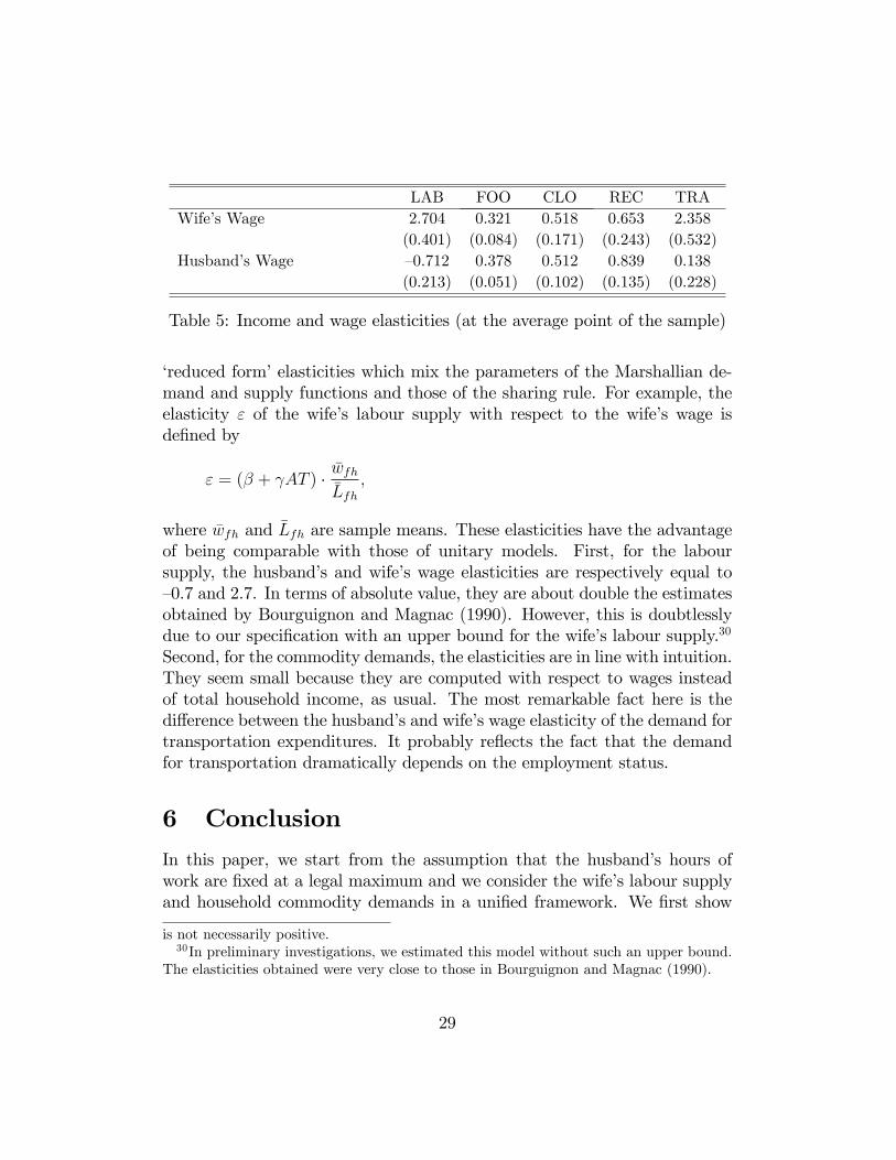
LAB FOO CLO REC TRAWife�s Wage 2.704 0.321 0.518 0.653 2.358

(0.401) (0.084) (0.171) (0.243) (0.532)Husband�s Wage �0.712 0.378 0.512 0.839 0.138

(0.213) (0.051) (0.102) (0.135) (0.228)

Table 5: Income and wage elasticities (at the average point of the sample)

�reduced form�elasticities which mix the parameters of the Marshallian de-mand and supply functions and those of the sharing rule. For example, theelasticity " of the wife�s labour supply with respect to the wife�s wage isde�ned by

" = (� + AT ) � �wfh�Lfh;

where �wfh and �Lfh are sample means. These elasticities have the advantageof being comparable with those of unitary models. First, for the laboursupply, the husband�s and wife�s wage elasticities are respectively equal to�0.7 and 2.7. In terms of absolute value, they are about double the estimatesobtained by Bourguignon and Magnac (1990). However, this is doubtlesslydue to our speci�cation with an upper bound for the wife�s labour supply.30

Second, for the commodity demands, the elasticities are in line with intuition.They seem small because they are computed with respect to wages insteadof total household income, as usual. The most remarkable fact here is thedi¤erence between the husband�s and wife�s wage elasticity of the demand fortransportation expenditures. It probably re�ects the fact that the demandfor transportation dramatically depends on the employment status.

6 Conclusion

In this paper, we start from the assumption that the husband�s hours ofwork are �xed at a legal maximum and we consider the wife�s labour supplyand household commodity demands in a uni�ed framework. We �rst show

is not necessarily positive.30In preliminary investigations, we estimated this model without such an upper bound.

The elasticities obtained were very close to those in Bourguignon and Magnac (1990).

29

that structural elements of the decision process can be identi�ed with theobservation of a single commodity demand function. Second, we generate aset of conditions that can be used to test the collective setting. Finally, weconclude with an empirical illustration using French data. These empiricalresults show that the structural parameters describing the intra-householddecision process and the husband�s behaviour are fairly well estimated.The rigidity of the husband�s labour supply is certainly a good approx-

imation for numerous countries. However, the validity of our method fordealing with this rigidity, compared to that in Blundell et alii (2001), is anempirical issue. We conjecture, nevertheless, that the approach we advo-cate is preferable for investigating female labour supply in France, where thelabour market is characterized by many job seekers.Nevertheless, several theoretical extensions (e.g., �xed costs of participa-

tion, nonlinear income taxation, or involuntary unemployment) are necessaryto properly assess the present setting. Above all, future research should con-centrate on the stochastic speci�cation and the functional form that we haveadopted. Speci�cally, the linearity of the wife�s labour supply is certainly asevere limitation. One serious problem here is that a more �exible speci�ca-tion does not allow us to recover a closed form for the shadow wages used toincorporate rationing in the model.

A List of Proofs

A.1 Proof of Proposition 1

If we di¤erentiate the wife�s labour supply function (3) with respect to y andwm and eliminate �

f�f; we obtain:

Lfy � �wm = Lfwm � �y. (14)

Then we use this equation to di¤erentiate the nth commodity demand func-tion along the locus de�ned by d� = 0. We simplify and obtain the husband�sEngel curve: �mn?�m = �

n. If we di¤erentiate this expression again with respectto y, wm and wf , we obtain:

�mn?�m�m � (1� �y) = �ny , (15)

�mn?�m�m � (1� �wm) = �nwm, (16)

��mn?�m�m � �wf = �nwf . (17)

30

Solving this system of partial di¤erential equations with (14) yields:

�wf = ��nwf�n, �wm = 1� �

nwm�

n, �y = 1� �ny�n and (18)

�mn?�m�m = (�n)�1: (19)

To retrieve �f�f and �fwf, we di¤erentiate the wife�s labour supply function

with respect to y, wm and wf , use (18), and rearrange to obtain :

�f�f =Lfwm � Lfy

(�nwm � �ny ) � �n and �fwf = Lwf +

Lfwm � Lfy(�nwm � �ny )

� �nwf . (20)

Similarly, we can di¤erentiate the nth commodity demand function withrespect to y, wm and wf , use (18), and rearrange to obtain:

�fn�f =�nwm �Qny � �ny �Qnwm

�nwm � �nyand �fnwf = Q

nwf�Qnwm �Qny�nwm � �ny

� �nwf :

Finally, knowing the sharing rule allows us to write down the wife�s actualbudget constraint and her preferences can be computed in the usual way. k

A.2 Proof of Proposition 2

If we introduce the derivatives of the wife�s labour supply function, given by(20), in the Slutsky Positivity condition, we obtain the �rst condition in thestatement of the proposition. If we di¤erentiate (19) with respect to y, wmand wf , and simplify, we obtain the second condition. k

A.3 Proof of Proposition 3

If we consider any pair of commodity demand functions, say n1 and n2; wehave a corresponding pair of systems of equations (15)�(17). If we simplify,we obtain the condition in the statement of the proposition. k

A.4 Proof of Proposition 4

The proof proceeds in stages. We prove that: (A) the sharing rule can beretrieved on the participation frontier, (B) this identi�cation can be extendedon int(N); and (C) testable restrictions are generated.

31

A) Frontier solution: Along the participation frontier, by the continuity ofthe wife�s labour supply function, we have the following identity:

�f [ (wm; y); �(wm; y)] = 0,

where �(wm; y) is in�nitely di¤erentiable. If we di¤erentiate this identity withrespect to wm and y and eliminate �

f�fand �fwf , we obtain:

y � �wm = wm � �y: (21)

Then we use this expression and di¤erentiate the nth commodity demandfunction along the direction d� = 0. We obtain the husband�s Engel curve:�mn?�m = A

n. We di¤erentiate this expression again to obtain:

�mn?�m�m � (1� �wm) = Anwm, (22)

�mn?�m�m � (1� �y) = Any : (23)

Finally, using (21) and solving this system yields:

�wm = 1� Anwm �Bn; �y = 1� Any �Bn and

�mn?�m�m = Bn: (24)

These equations de�ne the sharing rule up to an additive constant along theparticipation frontier.B) Interior solution: We di¤erentiate the nth commodity demand functionwith respect to wm; wf and y and eliminate �

mn?�m

and �fn?�f to obtain a partialdi¤erential equation in �wf , �wm and �y:

(Qnwm �Qny ) � �wf �Q

nwf� �wm +Q

nwf� �y = 0: (25)

From standard theorems of the partial di¤erential equation theory (e.g., John(1983)), the partial di¤erential equation (25) together with the speci�cationof the sharing rule on the boundary completely determines the wife�s share� for any (wf ; wm; y) 2 N , provided that a regularity condition is satis�ed.First, let us remark that the partial di¤erential equation (25) can be writtenas u � r� = 0, where r� is the gradient of � and u is the vector (Qnwm �Qny ;�Qnwf ; Q

nwf). Now, the condition is that the vector u is tangent to the

participation frontier. Since the equation of this frontier is wf � (wm; y)and given that, on the frontier, Q coincides with Qn, this condition becomes :Qnwm 6= Qny . Formally, this result is local rather than global and additionalconditions are required to identify the sharing rule on the entire set N .C) Constraints: Di¤erentiating (24) with respect to y and wm and simplifyingyields the condition in the statement of the proposition. k

32

B The Wage Equation

The wage equation includes, among the explanatory variables, the wife�seducation (measured in years), the square and the cube of this variable,the wife�s age, a cross-term of education and age, dummies for the wife�snationality (equal to one if it is di¤erent from French), for the region (Ruraland Paris) and for households with a telephone and an indicator of the labourmarket tension. The latter is de�ned as:

log

�number of job o¤ers by �rms

number of job demands by individuals

�for each French department. Several variables in the right-hand side of themarket wage regression are excluded from the empirical model of householdbehaviour. One important point is that, in order to obtain a greater precision,the wage equation is estimated with a large sample (1769 observations) whichalso includes households with more than one child. We see in Table 3 thatall the parameters are very signi�cant (with the expected sign). In principle,this permits identi�cation of the e¤ect of the wife�s wage since some of thevariables in the wage equation are excluded from the collective model in themain text. The coe¢ cient of determination is, however, quite small.

33

Estimates Std. Dev.Constant 175.9 46.5Wife�s Education �41.9 15.7Wife�s Education exp2 4.0 1.7Wife�s Education exp3 x 10e�3 �132.0 62.5Wife�s Age �10.2 2.5Wife�s Education � Wife�s Age x 10e�3 177.0 370.0Labour Market Tension �4.7 1.6Wife�s Nationality �7.5 1.8Paris Region 3.8 1.6Rural Region �2.3 1.1Presence of a Telephone 4.5 1.9Mill�s Ratio 4.0 1.7R2 0.09Number of Observations 1769

Table 6: Parameter Estimates of the Wage Equation

References

[1] Blundell R., P.-A. Chiappori, T. Magnac and C. Meghir (2001), �Col-lective Labour Supply: Heterogeneity and Nonparticipation�, WorkingPaper 01-19, Institute for Fiscal Studies.

[2] Bourguignon F., M. Browning and P.-A. Chiappori (1995), �The Collec-tive Approach to Household Behaviour�, Working Paper 95-04, DELTA.

[3] Bourguignon F., M. Browning, P.-A. Chiappori and V. Lechene (1993),�Intra-household Allocation of Consumption: A Model and Some Ev-idence from French Data�, Annales d�Economie et de Statistique 29:137-156.

[4] Bourguignon F. and T. Magnac (1990), �Labor Supply and Taxation inFrance�, Journal of Human Resources 25: 358-389.

[5] Browning M., Bourguignon F., P.-A. Chiappori and V. Lechene (1994),�Income and Outcomes: A Structural Model of intra-household Alloca-tion�, Journal of Political Economy, 102: 1067-1096.

34

[6] Browning M. and P.-A. Chiappori (1998), �E¢ cient Intra-household Al-locations: A Genenral Characterization and Empirical Tests�, Econo-metrica, 66: 1241-1278.

[7] Browning M. and C. Meghir (1991), �The E¤ects of Male and FemaleLabor Supply on Commodity Demands�, Econometrica, 59: 925-51.

[8] Chiappori P.A. (1988), �Rational Household Labor Supply�, Economet-rica, 56: 63-90.

[9] Chiappori P.A. (1992), �Collective Labor Supply and Welfare�, Journalof Political Economy, 100: 437-467.

[10] Chiappori P.A. (1997), �Introducing Household Production in CollectiveModels of Labor Supply�, Journal of Political Economy, 105: 191-209.

[11] Chiappori P.A. and I. Ekeland (2002a), �The Micro Economics ofGroup Behavior: General Characterization�, manuscript, University ofChicago.

[12] Chiappori P.A. and I. Ekeland (2002b), �The Micro Economics of GroupBehavior: Identi�cation�, manuscript, University of Chicago.

[13] Chiappori P.-A., Fortin B. and G. Lacroix (2002), �Marriage Market,Divorce Legislation and Household Labour Supply�, Journal of PoliticalEconomy, 110: 37-72.

[14] Donni O. (2003), �Collective Household Labor Supply: Nonparticipationand Income Taxation�, Journal of Public Economics, 87: 1179-1198.

[15] Fong Y. and Zhang J. (2001), �The Identi�cation of Unobservable In-dependent and Spousal Leisure�, Journal of Political Economy, 109:191-202.

[16] Fortin B. and G. Lacroix (1997), �A Test of the Unitary and CollectiveModels of Household Labour Supply�, Economic Journal, 107: 933-955.

[17] Hausman J. (1981). �Labor Supply�. In: Aaron H. and J. Pechman(eds), How Taxes A¤ect Economic behaviour,Washington D.C.: Brook-ing Institution.

35

[18] John F. (1983), Partial Di¤erential Equations, Springer Verlag, New-York.

[19] Kooreman P. and Kapteyn A. (1986), �Estimation of Rationed and Un-rationed Household Labour Supply Functions Using Flexible FunctionalForms�, Economic Journal, 96: 398-412.

[20] Laroque G. et Salanié B. (2002), �Labour Market Institutions ans Em-ployment in France�, Journal of Applied Econometrics, 17: 25-48.

[21] Lundberg S. et R Pollak (1996), �Bargaining and Distribution in Mar-riage�, Journal of Economic Perspectives, 10: 139-158.

[22] Neary J.P. and K.W.S. Roberts (1980), �The Theory of Household Be-haviour under Rationing�, European Economic Review, 13: 25-42.

[23] Vermeulen F., 2002, �Collective Household Models: Principles and MainResults�, Journal of Economic Surveys, 16: 533-564.

36