Collateral Values by Asset Class: Evidence from Primary ... · Collateral Values by Asset Class:...

Collateral Values by Asset Class: Evidencefrom Primary Securities Dealers

Leonardo BartoliniFederal Reserve Bank of New York

Spence HiltonFederal Reserve Bank of New York

Suresh SundaresanColumbia Business School

Christopher TonettiNew York University

Using data on repurchase agreements by primary securities dealers, we show that threeclasses of securities (Treasury securities, securities issued by government-sponsored agen-cies, and mortgage-backed securities) can be formally ranked in terms of their collateralvalues in thegeneral collateral(GC) market. We then show that GC repurchase agreement(repo) spreads across asset classes display jumps and significant temporal variation, espe-cially at times of predictable liquidity needs, consistent with the “safe haven” properties ofTreasury securities:These jumps are driven almost entirely by the behavior of the GC reporates of Treasury securities. Estimating the “collateral rents” earned by owners of these se-curities, we find such rents to be sizable for Treasury securities and nearly zero for agencyand mortgage-backed securities. Finally, we link collateral values to asset prices in a sim-ple no-arbitrage framework and show that variations in collateral values explain a signifi-cant fraction of changes in short-term yield spreads butnot those of longer-term spreads.Our results point to securities’ role as collateral as a promising direction of researchto improve understanding of the pricing of money market securities and their spreads.(JELG12, G23)

IntroductionFinancial securities derive their value from two sources: First and perhapsthe most important source of value is the promised cash flows by the issuer.We will refer to this source as the value derived from “cash flow rights.” The

We thank Michael Johannes and Tony Rodrigues for comments and suggestions, and Sam Cheung for out-standing research assistance. The views expressed here are those of the authors and do not necessarily reflectthose of the Federal Reserve Bank of New York or the Federal Reserve System. Send correspondence to SureshSundaresan, Columbia Business School, 3022 Broadway, Uris Hall 811, New York, NY 10027; telephone: (212)854-4423. E-mail: [email protected].

c© The Author 2010. Published by Oxford University Press on behalf of The Society for Financial Studies.All rights reserved. For Permissions, please e-mail: [email protected]:10.1093/rfs/hhq108 Advance Access publication October 18, 2010

Collateral Values by Asset Class: Evidence from Primary Securities Dealers

second source of value is the ability of the security to serve as collateral. Wewill refer to this source as value derived from “collateral rights.”1

Different classes of assets differ in these two sources of value. For exam-ple, Treasury securities have relatively high cash flow rights compared withother securities, given the high degree of certainty about future payment flows.Treasury securities as a class are also regarded by market participants as hav-ing excellent collateral rights. The relative homogeneity of Treasury securities,active secondary markets, absence of contractual complications such as pre-payments, and large issue sizes all contribute to their relatively high collateralvalue. Other types of financial instruments such as common stocks with smallcapitalization, as a class, are viewed as securities with relatively poor collat-eral rights. These characteristics, in addition to the certainty of future paymentflows, contribute to the widespread acceptance of Treasury securities as col-lateral, and enable institutions that borrow cash by posting these securities ascollateral to enjoy lower borrowing rates. Investors that would take possessionof such securities in the event of default could expect either to be able to liqui-date their holdings with relative ease at minimal loss (given active secondarymarkets), or to be able to borrow money more readily posting these securitiesas collateral.

The distribution of the value of a security between these two sources mayvary over time for a number of reasons: In periods of borrowing constraintsand aggregate liquidity shocks, it is reasonable to expect the collateral rightsof Treasury securities, as a class, to command a higher valuation. Likewise,in periods of abundant liquidity we may expect the collateral rights to be ofless value. In periods of aggregate financial distress, there may be a strongpreference to hold securities whose cash flow rights are not subject to default.Since such crises are usually also accompanied by insufficient access to credit,the value of collateral rights may also go up. Hence, we may expect to seea positive association between measures of collateral rights and the marketvalue of the securities. Furthermore, this correlation should be especially highin periods of aggregate liquidity shocks.

The goal of this article is to examine the time-series and cross-sectionalproperties of collateral rights of three distinct asset classes: Treasury, fed-eral agency debt securities, and agency mortgage-backed securities (MBSs).2

Specifically, we are the first to estimate the relative collateral values of differ-ent classes of securities (measured by the GC repurchase agreement [knownas repo] rate spreads) and their collateral rents (measured by the secured-unsecured rate spreads). In addition, we explore the extent to which differ-ences in the valuation of collateral rights may help explain the differences in

1 Securities such as common stock will also have “control rights.” We consider in our article only debt securitiesfor which control rights are unimportant.

2 The term MBS is used in the article to refer to agency mortgage-backed securities to the exclusion of private-label MBSs.

249

The Review of Financial Studies / v 24 n 1 2011

the overall valuation of these asset classes. We briefly motivate these questionsfurther below.

According to data from the Securities Industry and Financial Markets As-sociation (SIFMA), the securities dealers held on average $3.91 trillion of se-curities under repo and $2.59 trillion of cash under reverse repo arrangementsin the fourth quarter of 2008. As shown in Table1, primary dealers, for whichmore detailed data are available, rely especially heavily on repurchase agree-ments, favoring Treasury securities over agency and mortgage-backed securi-ties both in overnight and in term contracts.3 This dominance of Treasury repotransactions over agency and mortgage-backed securities should be viewed inthe context of the size of these underlying markets: TheSecurities Industryand Financial Markets Association(2009) reports that the size of the Treasurymarket as of the fourth quarter of 2008 was $6.1 trillion, whereas the fed-eral agency securities market was $3.2 trillion, and the MBS market stood at$8.9 trillion. As a proportion of the underlying market, repo financing in theTreasury market far exceeds the other markets. This may be driven by many of

Table 1Financing by Primary Securities Dealers (in billions of $)

Securities in January 2007 December 2007 August2008

U.S. TreasuryOvernight and continuing 1,280 1,471 1,467Term 1,105 1,302 1,352

Federal agency and GSEsOvernight and continuing 177 219 261Term 231 262 327

Mortgage-backedOvernight and continuing 140 172 193Term 406 460 425

CorporateOvernight and continuing 107 128 124Term 91 85 60

Securities out January 2007 December 2007 August2008

U.S. TreasuryOvernight and continuing 1,277 1,425 1,450Term 874 1,190 1,150

Federal agency and GSEsOvernight and continuing 320 399 485Term 145 158 222

Mortgage-backedOvernight and continuing 604 784 786Term 225 250 202

CorporateOvernight and continuing 302 363 304Term 77 89 75

Federal Reserve Bulletin, Statistical Supplement, Jun 2007, Mar 2008, Dec 2008. GSE = Government SponsoredEnterprise.

3 Data are fromStaff Publications Committee(2009). Primary dealers are designated counterparties to theFed’s open market operations. The current list of primary dealers is available atwww.newyorkfed.org/markets/pridealers current.html.

250


the same factors that lead market participants to regard Treasury securities ashaving excellent collateral rights.

Relevant LiteratureOne of the key themes in recent research on the role of collateral in the fund-ing of financial intermediaries has been to explain differences between rates onrepos against general collateral (GC) (which apply when any security withinan asset class can be used as collateral) and “special” repo rates (which ap-ply when only a specific security can be posted as collateral). One of thefirst contributions to this line of research is byCornell and Shapiro(1989),who document the price premium commanded by thirty-year Treasury bondsand show this premium to reflect, largely, low “special” repo rates in 1986.Similarly, Sundaresan(1994) documents that newly issued Treasury securi-ties tend to trade “special” in repo markets, with the extent of specialnessreflecting auction cycles.Duffie (1996) shows that the specialness in repo mar-kets should raise the price of the underlying security by the present value ofthe saving in borrowing costs in repo markets—a prediction supported em-pirically by Jordan and Jordan(1997). The latter paper also shows that theliquidity premium in newly issued Treasury securities reflects their special-ness in repo markets, with auction tightness and percentage awarded to dealersalso helping explain subsequent specialness in repo markets. More recently,Krishnamurthy(2002) documents the spread between newly issued and oldthirty-year Treasury bonds, also linking this spread to the difference in repomarket financing rates between the two bonds.4 Longstaff(2004) has shownthat Treasury securities have a significant “flight to liquidity” premium builtinto their market valuation. He demonstrates this by first estimating the spreadbetween Treasury bonds and otherwise similar bonds issued by Refco Inc.(Chicago, Illinois), and then showing that this spread may be as much as 15%of the value of the Treasury securities. He further examines the determinants ofthis spread. Our study complements the paper ofLongstaff(2004) by showingthat in episodes of flight to quality and liquidity, Treasury GC repo rates fallwell below the GC rates of other asset classes, thereby contributing further totheir increased value.

The role played by securities as collateral and their pricing implications havebeen stressed byBrunnermeir and Pedersen(2009), Garleanu and Pedersen(2009), andGeanakaplos(1997, 2003, 2009). Brunnermeir and Pedersen(2009)note that securities with identical cash flows can have substantiallydifferent margins due to differences in their current and potential secondarymarket liquidity.Garleanu and Pedersen(2009) argue that the equilibrium pric-ing of securities must reflect both their betas and their margins. In a series of

4 Two papers, byBindseil, Nyborg, and Strebulaev(2002, 2009), explore related issues using data on repos againstthe European Central Bank. However, the focus of these papers is less on estimating collateral values, and moreon auction-related themes, including bidding strategies and auction performance.

251


papers, Geanakaplos has explored the collateral values of securities and theirimplications for default, leverage, and pricing. InGeanakaplos(2009), supplyand demand determines both the equilibrium price (interest rates) and mar-gins (collateral value). The basic idea that margins are endogenous has beendeveloped inGeanakaplos(1997, 2003). These papers provide a theoreticalbackground and underpinning to some of our empirical results.

Contributions and Summary of ResultsA common feature of the extant literature in this area is its reliance on reporates drawn from the inter-dealer market for Treasury repos and—moreimportantly—its emphasis on spreads between rates on general and specialTreasury collateral. To our knowledge, rate spreads between repos on GC fordifferent classes of securities have not yet been investigated. There are manyreasons why the study of the financing rates across different asset classes is ofinterest. First, such an examination is valuable in as much as such an empiri-cal study can help us understand how financing rates of different asset classesvary over time and what factors may influence such time variation. In addi-tion, the relative values of different classes of collateral are likely to vary inways that shed light on the determinants of collateral values, such as financialintermediaries’ needs for liquidity, the need for cash investors to have liquidcollateral, and the extent of the demand in the market for protection (“safehaven”) against aggregate liquidity shocks. Finally, any variations in financingrates (over time and across asset classes) may have implications for asset pric-ing. For these reasons, in this article we undertake a comprehensive study ofthe longitudinal and cross-collateral properties of rates for GC repos, drawingon a newly available set of data on primary dealers’ repo activity provided bythe Federal Reserve Bank of New York. These data contain information on thesecured funding activities of primary securities dealers, including data on fi-nancing rates over a narrow daily window (the first hour of trading) for threedifferent classes of collateral: Treasury, agency, and mortgage-backed securi-ties. These data allow us to make contributions to the repo literature in severaldirections.

First, we compare rates on repos against Treasury securities with rates onrepos against agency and mortgage-backed securities, in order to evaluate dif-ferences in collateral values across the three asset classes. We find that Trea-sury repo rates are significantly (economically and statistically) lower thanthose of the other two asset classes. In our estimation (using data spanningour sample period of over seven years), the long-run average repo spreads be-tween agency and Treasury securities is 5.2 basis points, while that betweenmortgage-backed and Treasury securities is 6.1 basis points. The data in oursample cover the period from October 1999 to December 2006, and hence donot include the period of credit crisis. Economic intuition would suggest thatduring the crisis period, this effect should be much bigger. Indeed, during the

252


crisis, there were extended periods during which the GC repo rates of Treasurywere lower than the MBS GC repo rates by 100–300 basis points.5

Second, we document significant time-variation in the GC repo spreads,which often exhibit jumps around predictable liquidity dates (such as year-ends, quarter-ends, holidays, etc.) and random aggregate shocks. We use anestimation procedure to account for the possibility of jumps in repo spreadsaround predictable liquidity dates and random aggregate shocks and find thatrates on GC repos against Treasury collateral decline sharply relative to rateson GC repos against agency and mortgage-backed securities in periods of liq-uidity needs. This evidence is consistent with the view that Treasury securitiesincorporate a safe-haven premium relative to other securities.Our evidencefinds little or no increase in the GC repo rates of agency securities and MBScollateral relative to unsecured rates around such dates. This is an importantfinding, as any evidence of such an increase would have suggested that theincrease in GC repo spreads might be due to the perceived increase in creditrisk of the agency and mortgage-backed securities relative to the Treasury as aclass.6

Third, we extract collateral values of Treasury, federal agency, and mortgage-backed securities by calculating spreads between rates on GC repos for thesesecurities and matching rates on unsecured loans (federal funds rates) andstudy their dynamic properties. Consistent with the theoretical prior that own-ers of securities can borrow funds at a lower rate when pledging such securitiesas collateral, we document that Treasury securities display superior attributesas collateral and therefore command greater “collateral rents” by way of lowerrepo rates relative to the fed funds rate. Somewhat surprisingly, we find thatrepo rates against agency and mortage-backed securities are not meaningfullydifferent from rates on unsecured loans, a finding that suggests that agencyand mortgage-backed securities are used by their owners to obtain (or ex-pand) access to the short-term money market rather than to gain financing priceadvantages.

Finally, we develop a simple no-arbitrage relationship between the repospreads of assets and their yield spreads. Our model predicts that yield spreadsshould capture the present value of the stream of future repo spreads. Usingour estimated parameters, we evaluate the predictions of our model. Consis-tent with the view that in an efficient market the desirability of a security as acollateral should be fully incorporated in its price,7 we find that repo spreadshelp explain a significant percentage of the yield spreads for short (money mar-ket) maturities. However, we find GC repo spreads to play a negligible role indetermining longer-term yield spreads.

5 Data confirming this can be found in theMarkets Group of the Federal Reserve Bank of New York(2009)publication concerning the open market operations of 2008.

6 We thank the referee for alerting us to this potential alternative explanation.

7 For detailed analysis, in the context of Treasury securities, seeDuffie (1996).

253


The article is organized as follows. Section1 reviews the market for repur-chase agreements against general collateral. Section2 explains the data used inour study and presents summary statistics and preliminary empirical evidence.Section3 formulates our formal empirical model of collateral spreads and val-ues, discusses its estimation, and presents our main findings. Section4 linkscollateral values to pricing spreads through a simple arbitrage argument andverifies the empirical relevance of such a link. Section5 concludes.

1. The Market for General Collateral Repo

The term “repurchase agreement” identifies a transaction in which an investor(the “repo borrower”of cash) acquires funds by selling securities to another in-vestor (the “repo lender”of cash), simultaneously agreeing to repurchase thosesecurities at a future time at a specified price, where the excess over the ini-tial sale price reflects the interest on the loan.8 Albeit technically defined aspurchases and matched forward sales of securities, for most practical purposesrepos can be thought of as collateralized loans. Certain features of repo agree-ments do indeed confirm this analogy, such as the practice of assigning anycoupon that might be payable during the term of the repo (along with fullaccrual of interest) to the repo borrower (i.e., to the original owner of the se-curity) rather than to the repo lender (the temporary owner of the security).Other features of repo contracts, however, align repos more closely to securi-ties sales, such as the right acquired by repo lenders to immediately liquidatethe collateral in case of default on the underlying loan.

GC repos differ from “special collateral” repos in that for the latter case, aspecific security is designated as the only acceptable collateral, whereas withGC repos, a certain designated class of securities are acceptable. The cash bor-rower has the option to deliver as collateral any securities that fall within thatclass. Borrowers of cash in the GC repo market are often financing a portfolioof securities, while lenders of cash are looking for a safe investment that of-fers market-based rates of return. Indeed, the market for GC repos has growninto one of the main channels for funding of U.S. financial institutions in re-cent years and short-term lending of excess cash balances. GC repos typicallycarry a short maturity. Most are arranged with terms of one to a few days, orstandard terms of one, two, or three weeks, or one, two, three, or six months.9

Dollar amounts tend to be large, usually exceeding $25 million per trade forshort maturities and $10 million for longer-term repos.

8 Whether a specific transaction is termed a repo or a reverse repo usually depends on the perspective of theborrower or lender of the cash or securities. For the borrower of cash (lender of securities) these transactions arecalled “repos,” and “reverse repos” for the lender of cash (borrower of securities).

9 While most repos are standardized along these lines, “open” repos (i.e, open-ended, multi-day contracts) arealso traded, as well as “continuing” repos that are renewed each day upon agreement by both parties, allowingfor adjustment in both the repo rate and the amount of funds invested.

254


A key distinction in GC repo transactions hinges on the type of collat-eral underlying the transaction. The class of acceptable collateral may includeall Treasury securities or certain private sector securities, or it could be re-stricted to a subset of such securities, such as those maturing in less than tenyears. In practice, Treasury securities account for a large share of this mar-ket, but there is a very active market also for repos against securities issued bygovernment-sponsored agencies and agency mortgage-backed securities. Thevery short-term nature of the GC repo data (overnight) and the admissibility ofa designated class of securities allows us to shed some light on the differencesin collateral value of different asset classes.

Different settlement procedures tend to dominate different segments of theGC repo market.10 The repo data used in this study largely reflect transactionsbetween the Fed’s primary dealers and their biggest retail customers, such asmoney market mutual funds and other large institutional investors that haveconsiderable quantities of cash to invest each day. In this segment of the mar-ket, “tri-party” agreements are typically used to settle GC repo transactions, forwhich both the (cash) borrower and lender maintain a securities account anda deposit account at a clearing bank.11 When a tri-party repo transaction firstsettles (or unwinds), the clearing bank will move funds and securities betweenthe respective cash and custody accounts of the borrower and lender. Clearingbanks also provide other services, such as valuation of collateral.

GC repo transactions are not necessarily risk free, even if the cash flow ofthe underlying security is free of default risk. Specifically, if the (cash) bor-rower fails to repurchase the securities at term, in which case the (cash) lenderkeeps the security, the lender is exposed to the risk of a change in the se-curity’s value due to market movements as well as the risk of being unableto liquidate the securities as needed. To mitigate the risk that the (cash) bor-rower fails to return the funds, repos are normally over-collateralized, by re-quiring the market value of the underlying collateral to exceed the amount ofthe loan, and they are subject to daily mark-to-market margining. The over-collateralization factor (“haircut”) normally depends on the term of the repo,the liquidity of the underlying security, and the strength of the counterpartiesinvolved. Haircuts tend to be larger as the interest sensitivity of the underlyingsecurity’s price increases—hence, they tend to rise with the term to maturityof the underlying securities. They also tend to rise with credit risk—hence,they are higher for private instruments than comparable Treasury securities.Herring and Schuermann(2005) note that “for U.S. government and agencyinstruments, the haircuts are the most modest. They range from 0 percent forvery short-term (0–3 months) to 6 percent for long-term (>25 years) debt.”With the onset of the credit crisis in August 2007, haircuts have changed, even

10 Detailed descriptions of some of the types of settlement practices used by the primary dealers and recentinnovations are found inFleming and Garbade(2002, 2003).

11 The two largest clearing banks that dominate this business are JPMorgan Chase and Bank of New York.

255


for Treasury securities. Our understanding is that the haircuts have becomemuch higher at times even for federal agency securities relative to Treasuries.Unfortunately, we do not have data for this period.12

2. GC Repo Spreads: Data and Summary Evidence

In this section, we briefly describe the sources and nature of our data. We thenpresent some summary evidence on the behavior of GC repo spreads acrossthe three asset classes.

2.1 DataThe core data for our study are the Federal Reserve Bank of New York’s dailydata on overnight repurchase agreements contracted by Government SecuritiesPrimary Dealers with their retail customers between about 8:00 and 8:45 a.m.,from October 12, 1999, to December 25, 2006.13

The data that we obtained are collected by the Federal Reserve Bank of NewYork as part of a daily survey of the primary dealers,14 and include volume-weighted averages of rates paid by all current dealers in the GC repo marketwith their retail customers, such as money market funds, since the open ofbusiness that day, broken down by three classes of general collateral: Treasurysecurities, securities issued by government-sponsored agencies, and mortgage-backed securities. To our knowledge, the Fed’s survey of primary dealers is theonly systematic source of data on dollar GC repurchase agreements. This lackof data reflects the fact that—unlike special repos, which trade largely on elec-tronic platforms like BrokerTec—the GC market trades mostly through voicebrokers, who tend to keep limited information archived in usable electronicform. A noteworthy feature of our data is that their morning sampling timeof retail repo transactions tends to be earlier in the day than when most inter-dealer trades are executed. Nonetheless, rates in these two market segments areclosely bound together, as inter-dealer trading in general collateral securities isused to balance mismatches in flows between individual dealers and their retailcustomers.

12 When short-term interest rates are very low, there may be an incentive to “fail” in repo transactions. In “TreasuryMarket Best Practices,” theTreasury Market Practices Group(2009) reports that a “fails charge” has beeninstituted, reducing the incentive to fail.

13 These data are highly confidential and were provided to the authors under tightly controlled circumstances.Regrettably, the data that we obtained did not include the interesting crisis period that began in the summer of2007. However, it would be of great interest to extend our methodological contribution to a sample inclusive ofa major crisis period, should the required data become available in the future.

14 Altogether, 31 different dealers were surveyed over our sample period, with an average of 24 surveyed on anygiven day. Variability during the sample in the number of surveyed dealers reflects almost entirely changes inthe number of eligible dealers, caused by mergers and acquisitions among dealers and a few entries or exits bycertain institutions in the pool of primary dealers.

256


In addition to our key data on repurchase agreements, other data we usedinclude constant-maturity bond rates for Treasury securities (obtained from theBoard of Governors of the Federal Reserve) and agency securities (obtainedfrom Fannie Mae). We also obtained series of 9:00 a.m. federal funds ratesfrom the Federal Reserve Bank of New York, and Nelson-Siegel-Svenssondiscount rates from the Board of Governors of the Federal Reserve (the latterdata are discussed in detail byGurkaynak, Sack, and Wright 2007). Finally,from Michael Fleming and Neel Krishnan at the Federal Reserve Bank of NewYork, we obtained average daily bid-ask spreads between 8:00 and 9:00 a.m.for the on-the-run two-year note, from January 1, 2001, to February 3, 2006,calculated from transaction-level BrokerTec data.

2.2 Summary EvidenceSummary information on our repo data is displayed in Table2. The raw dataseries are shown in Figures1 and2, while frequency distributions of the se-ries are plotted in Figures3 and4. Much economic intuition can be gained byobserving the raw data spreads. The key information displayed in the table con-sists of raw means and volatilities of spreads between (daily, volume-weighted)rates on repos against different classes of collateral and spreads between unse-cured (federal funds) and secured (repo) rates. The highlight of the table is thestrict order among the three classes of collateral: When posting Treasury secu-rities as collateral, repo borrowers can obtain financing at rates 6 basis pointslower, on average, than when posting agency securities, and at rates 7 pointslower than when posting MBSs. The ordering is clearly statistically significant,as the 95% confidence interval for the estimated mean of the Treasury-agencyspread is [−6.25,−5.76], while that for the agency-MBS spread is [−1.07,−0.94].

Another feature displayed by our collateral spreads is the excess of meanover median spreads, suggesting a right-tailed distribution that may reflectlarge spreads during episodes of flight to quality. This conjecture is informallyconfirmed by the large and asymmetric ranges between highest and lowestspreads around mean spreads displayed in Table2.

Table 2Federal Reserve’s Dealer Survey: Summary Information

Sample 10/13/1999 – 1/25/ 2006# of observations (# business days) 1,562

Spreads Mean Median Standard deviation MinimumMaximum

Treasury repo – Agency repo −6.00 −4.67 4.87 −78.87 −1.22Treasury repo – Mortgage-backed repo−7.01 −5.54 5.68 −97.87 −1.88Agency repo – Mortgage-backed repo−1.01 −0.83 1.34 −42.34 1.55Federal funds – Treasury repo 7.50 5.36 9.94 −4.60 263.45Federal funds – Agency repo 1.50 0.73 6.86 −25.18 207.92Federal funds – Mortgage-backed repo 0.49 −0.24 5.98 −29.70 166.58

All spreads are in basis points and computed as differences between daily volume-weighted rates.

257


Figure 1Spreads between repo rates against different collateral

Figure 2Spreads between unsecured (federal funds) and repo rates

258


Figure 3Frequency distributions of spreads between repo rates against different collateral

Figure 4Frequency distributions of spreads between unsecured (federal funds) and repo rates

259


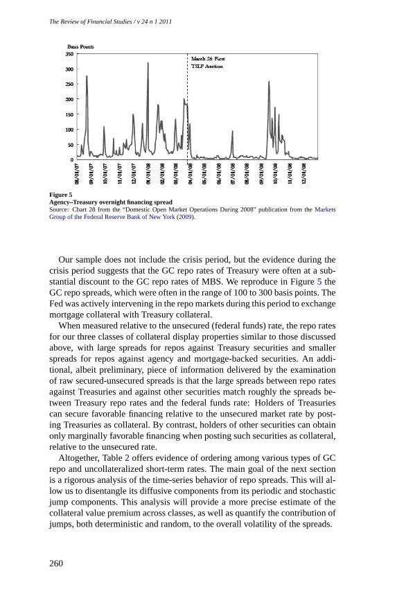
Figure 5Agency–Treasury overnight financing spreadSource: Chart 28 from the “Domestic Open Market Operations During 2008” publication from theMarketsGroup of the Federal Reserve Bank of New York(2009).

Our sample does not include the crisis period, but the evidence during thecrisis period suggests that the GC repo rates of Treasury were often at a sub-stantial discount to the GC repo rates of MBS. We reproduce in Figure5 theGC repo spreads, which were often in the range of 100 to 300 basis points. TheFed was actively intervening in the repo markets during this period to exchangemortgage collateral with Treasury collateral.

When measured relative to the unsecured (federal funds) rate, the repo ratesfor our three classes of collateral display properties similar to those discussedabove, with large spreads for repos against Treasury securities and smallerspreads for repos against agency and mortgage-backed securities. An addi-tional, albeit preliminary, piece of information delivered by the examinationof raw secured-unsecured spreads is that the large spreads between repo ratesagainst Treasuries and against other securities match roughly the spreads be-tween Treasury repo rates and the federal funds rate: Holders of Treasuriescan secure favorable financing relative to the unsecured market rate by post-ing Treasuries as collateral. By contrast, holders of other securities can obtainonly marginally favorable financing when posting such securities as collateral,relative to the unsecured rate.

Altogether, Table2 offers evidence of ordering among various types of GCrepo and uncollateralized short-term rates. The main goal of the next sectionis a rigorous analysis of the time-series behavior of repo spreads. This will al-low us to disentangle its diffusive components from its periodic and stochasticjump components. This analysis will provide a more precise estimate of thecollateral value premium across classes, as well as quantify the contribution ofjumps, both deterministic and random, to the overall volatility of the spreads.

260


3. The Empirical Behavior of GC Repo Spreads

3.1 Empirical modelIt is well known that money market interest rates and spreads exhibit season-ality. This has been documented by a number of scholars, includingMusto(1997) in the context of the rates on commercial paper, andSundaresan andWang(2009) in the context of the spreads between repo rates and target fedfunds rates. The latter paper shows that the volatility of the spreads is muchhigher in quarter-ends. Therefore, in this section we specify a process for theevolution of the spreads that allows for the possibility of jumps in the levelsof the spreads at predictable dates (such as quarter-ends, holidays, year-ends,etc.) as well as random future dates when there may be an aggregate liquidityshock. In addition, we allow for the possibility of stochastic volatility in thespreads. To this end, we first begin by defining spreads and interpreting theireconomic meaning.

3.2 Definition of spreadsTo investigate the time-series and cross-sectional behavior of repo rates, wedefine the following set of interest-rate spreads. First, let the repo spreads

STRE−AGEt ≡ r TRE

t − r AGEt (1)

STRE−MBSt ≡ r TRE

t − r MBSt (2)

SAGE−MBSt ≡ r AGE

t − r MBSt (3)

denote the spreads between the overnight rates on repurchase agreementsagainst Treasury (TRE), agency (AGE), and mortgage-backed (MBS) securi-ties, respectively.15

Second, let the secured-unsecured spreads

SFF−TREt ≡ r FF

t − r TREt (4)

SFF−AGEt ≡ r FF

t − r AGEt (5)

SFF−MBSt ≡ r FF

t − r MBSt (6)

denote the spreads between the contemporaneous rate on (unsecured) loans ofovernight federal funds and the three repo rates. (As noted above, our federalfunds rates were sampled almost contemporaneously to the repo data, withthe former capturing conditions just before 9:00 a.m., and the latter capturingconditions at 8:00–8:45 a.m.)

Note that the secured-unsecured spreads effectively measure the “collateralrents” earned by the owners of the relevant security. Intuitively, such ownerscan post the security as collateral to borrow cash overnight at the current GC

15 The notationr TREt is used to denote the overnight GC repo rate applicable to Treasury collateral, and so on. We

user FFt to denote the overnight effective fed funds rate.

261


rate while lending those funds overnight in the unsecured market at the cur-rent unsecured rate. Thus, the income earned on this position equals the spreadbetween the secured and unsecured rates or, equivalently, measures the oppor-tunity cost incurred by the security’s owner, should he choose to hold on to thesecurity instead of lending it out.

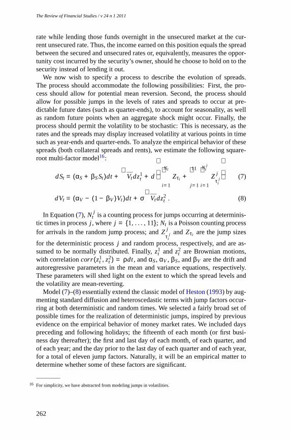
We now wish to specify a process to describe the evolution of spreads.The process should accommodate the following possibilities: First, the pro-cess should allow for potential mean reversion. Second, the process shouldallow for possible jumps in the levels of rates and spreads to occur at pre-dictable future dates (such as quarter-ends), to account for seasonality, as wellas random future points when an aggregate shock might occur. Finally, theprocess should permit the volatility to be stochastic: This is necessary, as therates and the spreads may display increased volatility at various points in timesuch as year-ends and quarter-ends. To analyze the empirical behavior of thesespreads (both collateral spreads and rents), we estimate the following square-root multi-factor model16:

dSt = (αS+ βSSt )dt +√

Vtdz1t + d

Nt∑

i=1

Zτi +11∑

j=1

N jt∑

i=1

Z j

τj

i

(7)

dVt = (αV − (1− βV )Vt )dt + σ√

Vtdz2t . (8)

In Equation (7), N jt is a counting process for jumps occurring at determinis-

tic times in processj , wherej = {1, . . . , 11}; Nt is a Poisson counting processfor arrivals in the random jump process; andZ j

τj

i

and Zτi are the jump sizes

for the deterministic processj and random process, respectively, and are as-sumed to be normally distributed. Finally,z1

t and z2t are Brownian motions,

with correlationcorr(z1t , z

2t ) = ρdt, andαS, αV , βS, andβV are the drift and

autoregressive parameters in the mean and variance equations, respectively.These parameters will shed light on the extent to which the spread levels andthe volatility are mean-reverting.

Model (7)–(8) essentially extend the classic model ofHeston(1993) by aug-menting standard diffusion and heteroscedastic terms with jump factors occur-ring at both deterministic and random times. We selected a fairly broad set ofpossible times for the realization of deterministic jumps, inspired by previousevidence on the empirical behavior of money market rates. We included dayspreceding and following holidays; the fifteenth of each month (or first busi-ness day thereafter); the first and last day of each month, of each quarter, andof each year; and the day prior to the last day of each quarter and of each year,for a total of eleven jump factors. Naturally, it will be an empirical matter todetermine whether some of these factors are significant.

16 For simplicity, we have abstracted from modeling jumps in volatilities.

262


3.3 Estimation approachWe estimated Model (7)–(8) using Markov chain Monte Carlo (MCMC)simulation techniques. For details of the properties of MCMC estimation, seeJohannes and Polson(2006).17 In essence, MCMC is used in Bayesian estima-tion to allow consistent and computationally efficient estimation of complexmodels such as (7)–(8), and delivers parameter estimates along with their es-timated probability distributions. MCMC estimation involves first discretizingthe model. (Results in the MCMC literature show that choosing sufficientlyshort intervals, such as one day, is generally sufficient to eliminate discretiza-tion bias.) Second, suitable conjugate prior distributions for the parameters arechosen. (Similarly, standard results ensure that the priors do not matter for es-timation results for informative well-behaved likelihood functions.) Third, thehigh-dimension likelihood function is partitioned into lower-dimension con-ditional distributions (with standard results, namely, the Clifford-HammersleyTheorem, ensuring that the joint posterior likelihood is completely character-ized by its conditional components). Fourth, values are drawn (this is theMonteCarlo stage) from the prior distribution using Model (7)–(8). Fifth, Bayesianupdating is used to generate posterior distributions for the parameters allow-ing the draw/update process (fourth and fifth steps) to be replicated iteratively,yielding aMarkov chainof values for the parameter set. The process is iterateda sufficient number of times (100,000 times, in our case) to secure convergenceto the unconditional distribution. The last-iteration posterior conditional distri-bution provides an estimate of the distribution of the parameter values and canbe used for inference. In our case, the estimation delivers at the same time anestimate of the latent volatility process and an estimate of individual jumps.

3.4 Results from estimationWe first present and discuss the results on collateral spreads across asset classesand then turn to an analysis of the collateral rents.

3.4.1 Collateral spreads. Tables3–5 summarize the estimated behavior ofthe collateral spreadsSTRE−AGE

t , STRE−MBSt , andSAGE−MBS

t .The large number of observations allows us to estimate the parameters of

both mean and variance processes with precision. As a preliminary matter,the estimatedβS andβV coefficients (negative the former, smaller-than-onethe latter) imply the stability of the mean and variance processes for all threespreads.

A key role in our analysis is played by the jump factors, estimates of whichare shown in the mid-panels of Tables3–5. Comparing the mean jumps acrossthe three tables reveals a number of stylized facts.

17 SeeJacquier, Polson, and Rossi(1994) for an example of estimating stochastic volatility models. SeeEraker,Johannes, and Polson(2003) for an example of estimating models with jumps in level and volatility.

263


Table 3Treasury–Agency Spread Estimation

Diffusion coefficients Estimates

αS −0.544(0.044)βS −0.139(0.010)αV 0.038(0.007)βV 0.970(0.006)σ 0.205(0.026)ρ −0.118(0.052)

Jump coefficients Mean jump Variance of jump Arrival Intensity Share of estimated variance

Random jump −4.416(2.604) 8.414(1.269) 0.010(0.003) 0.090Before holiday −0.226(0.264) 1.602(0.173) – 0.014After holiday −0.167(0.261) 1.579(0.69) – 0.01415th −0.649(0.226) 1.568(0.162) – 0.015First day of month 0.975(0.300) 1.781(0.203) – 0.020Month end −1.579(0.308) 1.856(0.211) – 0.022Before quarter end −1.342(0.728) 2.969(0.596) – 0.018Quarter end −7.194(2.103) 11.915(2.106) – 0.297After quarter end 5.769(1.991) 10.953(2.854) – 0.251Before year end −3.283(2.070) 5.859(1.678) – 0.020Year end −4.701(2.814) 5.347(2.959) – 0.017After year end 4.851(3.060) 9.785(6.664) – 0.056All jumps 0.832

Long run mean spreads −5.176(0.448)95% confidence interval: [−5.92,−4.44]99% confidence interval: [−6.25,−4.14]

The table reports results of MCMC estimation of the model. Standard errors are reported in parentheses, andare computed from the estimated posterior distribution of the coefficients. The sample includes 1,562 dailyobservations from October 13, 1999, to January 25, 2006.

Table 4Treasury–MBS Spread Estimation


αS −0.606(0.061)βS −0.132(0.011)αV 0.058(0.040)βV 0.969(0.008)σ 0.225(0.041)ρ −0.123(0.052)


Random jump −5.472(3.814) 10.286(1.604) 0.009(0.004) 0.087Before holiday −0.161(0.313) 1.849(0.218) – 0.012After holiday −0.296(0.315) 1.854(0.210) – 0.01315th −0.827(0.270) 1.824(0.194) – 0.014First day of month 1.198(0.340) 1.999(0.237) – 0.017Month end −1.804(0.354) 2.068(0.239) – 0.018Before quarter end −1.242(0.810) 3.276(0.624) – 0.015Quarter end −7.243(2.384) 14.648(2.773) – 0.301After quarter end 5.699(1.987) 10.448(3.250) – 0.153Before year end −3.531(2.206) 6.472(1.835) – 0.016Year end −4.363(2.945) 6.917(4.321) – 0.019After year end 3.378(3.274) 20.661(8.702) – 0.168All jumps 0.833

Long run mean spreads −6.108(0.547)95% confidence interval: [−7.02,−5.23]99% confidence interval: [−7.43,−4.85]


264


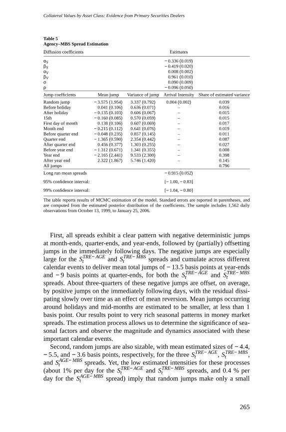
Table 5Agency–MBS Spread Estimation


αS −0.336(0.019)βS −0.419(0.020)αV 0.008(0.002)βV 0.961(0.010)σ 0.090(0.009)ρ −0.096(0.050)


Random jump −3.575(1.954) 3.337(0.792) 0.004(0.002) 0.039Before holiday 0.041(0.106) 0.636(0.071) – 0.016After holiday −0.135(0.103) 0.606(0.067) – 0.01515th −0.160(0.085) 0.570(0.059) – 0.015First day of month 0.138(0.106) 0.607(0.069) – 0.017Month end −0.215(0.112) 0.641(0.076) – 0.019Before quarter end −0.048(0.235) 0.857(0.145) – 0.011Quarter end −1.365(0.590) 2.354(0.442) – 0.087After quarter end 0.456(0.377) 1.303(0.255) – 0.027Before year end −1.312(0.671) 1.341(0.355) – 0.008Year end −2.165(2.441) 9.533(2.300) – 0.398After year end 2.322(1.867) 5.746(1.420) – 0.145All jumps 0.796

Long run mean spreads −0.915(0.052)

95% confidence interval: [−1.00,−0.83]

99% confidence interval: [−1.04,−0.80]


First, all spreads exhibit a clear pattern with negative deterministic jumpsat month-ends, quarter-ends, and year-ends, followed by (partially) offsettingjumps in the immediately following days. The negative jumps are especiallylarge for theSTRE−AGE

t and STRE−MBSt spreads and cumulate across different

calendar events to deliver mean total jumps of−13.5 basis points at year-endsand−9 basis points at quarter-ends, for both theSTRE−AGE

t and STRE−MBSt

spreads. About three-quarters of these negative jumps are offset, on average,by positive jumps on the immediately following days, with the residual dissi-pating slowly over time as an effect of mean reversion. Mean jumps occurringaround holidays and mid-months are estimated to be smaller, at less than 1basis point. Our results point to very rich seasonal patterns in money marketspreads. The estimation process allows us to determine the significance of sea-sonal factors and observe the magnitude and dynamics associated with theseimportant calendar events.

Second, random jumps are also sizable, with mean estimated sizes of−4.4,−5.5, and−3.6 basis points, respectively, for the threeSTRE−AGE

t , STRE−MBSt ,

andSAGE−MBSt spreads. Yet, the low estimated intensities for these processes

(about 1% per day for theSTRE−AGEt and STRE−MBS

t spreads, and 0.4 % perday for theSAGE−MBS

t spread) imply that random jumps make only a small

265


contribution to explaining the total variance of the spread processes: The shareof the estimated variance of the spread attributed to random jumps ranges be-tween 4% and 9% across the three spreads, as shown in the rightmost columns(mid-panel) in Tables3–5. This small contribution is especially surprisingwhen considering that random jumps can occur every day other than days as-signed to deterministic jumps. By contrast, the deterministic jumps explainabout 75% of the estimated variance of all spreads, with jumps occurringaround ends of months/quarters/years alone accounting for over 70% of the es-timated variances. Thus, flight-to-quality effects at predictable calendar timesare apparent and are estimated to dominate the dynamics of our collateralspreads. The term “flight-to-quality” refers to two distinct classes of eventsin our article. First, it refers to panics in the market that cause investors torush into Treasury securities over (and to some degree from) other securitiesconsidered in this article. Second, it refers to the demands that arise in quarter-ends and year-ends in order for institutions to achieve certain balance-sheetoutcomes for reporting purposes. Both classes of events refer to situationswhere institutions prefer to hold higher-quality and more-liquid instruments.A finding of our article is that both types of events are of economic interest,in general. Their relative importance may vary with the state of the financialmarkets. For example, our sample period did not cover the credit crisis periodduring which the random jumps in the GC repo spreads might have dominated.Indeed, we have alluded in the introduction to some evidence that suggests thatthis was the case.

We can summarize much of the insight from our estimation by presentingestimated unconditional (long-run) means of the spread processes, which aredisplayed in the lower panels of Tables3–5 with their standard errors.18 Theestimated unconditional means confirm that our three classes of collateralfollow a clear pecking order: Repo financing against Treasury securities isavailable at 5.2 basis points less than against agency securities and at 6.1 lessthan against MBSs. (The numerically computed confidence intervals displayedin the table show that these spreads are statistically significant at any standardconfidence level.)

3.4.2 Collateral rents. What determines the value of the collateral spreadsbetween Treasury and agency/mortgage-backed securities? To address thisquestion with regard to both dynamics and long-run trends, we use the unse-cured rates to investigate the empirical behavior of the collateral rentsSFF−TRE

t ,SFF−AGE

t , and SFF−MBSt , following the same methodology we used to study

collateral spreads in the previous section.Results of our estimation are presented in Tables6–8. The estimation has

two highlights: explaining the time variation in the collateral spreads through

18 Since the spread processes modeled by Equation (7) are affine, the unconditional means are easy to computeanalytically; however, their standard errors must be obtained numerically, as part of the MCMC simulations.

266


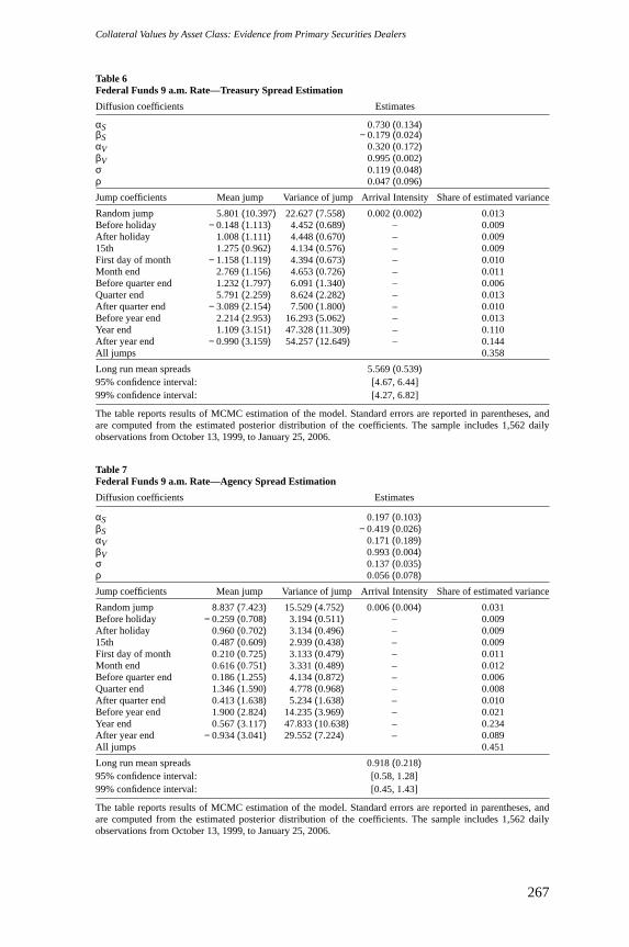
Table 6Federal Funds 9 a.m. Rate—Treasury Spread Estimation


αS 0.730(0.134)βS −0.179(0.024)αV 0.320(0.172)βV 0.995(0.002)σ 0.119(0.048)ρ 0.047(0.096)


Random jump 5.801(10.397) 22.627(7.558) 0.002(0.002) 0.013Before holiday −0.148(1.113) 4.452(0.689) – 0.009After holiday 1.008(1.111) 4.448(0.670) – 0.00915th 1.275(0.962) 4.134(0.576) – 0.009First day of month −1.158(1.119) 4.394(0.673) – 0.010Month end 2.769(1.156) 4.653(0.726) – 0.011Before quarter end 1.232(1.797) 6.091(1.340) – 0.006Quarter end 5.791(2.259) 8.624(2.282) – 0.013After quarter end −3.089(2.154) 7.500(1.800) – 0.010Before year end 2.214(2.953) 16.293(5.062) – 0.013Year end 1.109(3.151) 47.328(11.309) – 0.110After year end −0.990(3.159) 54.257(12.649) – 0.144All jumps 0.358

Long run mean spreads 5.569(0.539)95% confidence interval: [4.67, 6.44]99% confidence interval: [4.27, 6.82]


Table 7Federal Funds 9 a.m. Rate—Agency Spread Estimation


αS 0.197(0.103)βS −0.419(0.026)αV 0.171(0.189)βV 0.993(0.004)σ 0.137(0.035)ρ 0.056(0.078)


Random jump 8.837(7.423) 15.529(4.752) 0.006(0.004) 0.031Before holiday −0.259(0.708) 3.194(0.511) – 0.009After holiday 0.960(0.702) 3.134(0.496) – 0.00915th 0.487(0.609) 2.939(0.438) – 0.009First day of month 0.210(0.725) 3.133(0.479) – 0.011Month end 0.616(0.751) 3.331(0.489) – 0.012Before quarter end 0.186(1.255) 4.134(0.872) – 0.006Quarter end 1.346(1.590) 4.778(0.968) – 0.008After quarter end 0.413(1.638) 5.234(1.638) – 0.010Before year end 1.900(2.824) 14.235(3.969) – 0.021Year end 0.567(3.117) 47.833(10.638) – 0.234After year end −0.934(3.041) 29.552(7.224) – 0.089All jumps 0.451

Long run mean spreads 0.918(0.218)95% confidence interval: [0.58, 1.28]99% confidence interval: [0.45, 1.43]


267


Table 8Federal Funds 9 a.m. Rate—MBS Spread Estimation


αS −0.234(0.114)βS −0.452(0.021)αV 0.105(0.159)βV 0.991(0.005)σ 0.190(0.062)ρ 0.085(0.064)


Random jump 11.131(5.620) 13.441(3.028) 0.005(0.003) 0.038Before holiday −0.238(0.546) 2.740(0.385) – 0.012After holiday 0.916(0.540) 2.621(0.379) – 0.01115th 0.329(0.451) 2.464(0.315) – 0.011First day of month 0.393(0.561) 2.699(0.371) – 0.014Month end 0.301(0.602) 2.918(0.422) – 0.016Before quarter end 0.077(1.011) 3.483(0.685) – 0.008Quarter end 0.308(1.415) 4.522(0.934) – 0.013After quarter end 0.876(1.440) 4.873(1.166) – 0.015Before year end 1.792(2.786) 14.084(3.528) – 0.035Year end 0.607(3.085) 38.590(8.632) – 0.266After year end −1.049(2.987) 21.778(5.512) – 0.085All jumps 0.525

Long run mean spreads −0.162(0.262)

95% confidence interval: [−0.50, 0.36]

99% confidence interval: [−0.59, 0.52]


the jump behavior of the time series and the long-run determination of the col-lateral spreads through the unconditional means. First, consider the estimateddeterministic jumps for the three seriesSFF−TRE

t , SFF−AGEt , and SFF−MBS

t ,which we have seen play a critical role in the volatility of the collateral spreads.While deterministic jumps in theSFF−TRE

t spread are large and comparable inmagnitude to those estimated for theSTRE−AGE

t andSTRE−MBSt spreads, the de-

terministic jumps for theSFF−AGEt andSFF−MBS

t spreads are generally small.For instance, the cumulative mean of end-month, end-quarter, and end-yearjumps in theSFF−TRE

t spread is 9.7 basis points, while it is only 2.5 basispoints for theSFF−AGE

t spreads, indicating that agency-backed borrowing ratesfollow the unsecured rate much more closely.

The smallSFF−AGEt jumps suggest that theSTRE−AGE

t spread is econom-ically driven by changes in the collateral value of Treasury bonds. To dis-entangle whether the higher financing spreads observed around end-months,end-quarters, and end-years are driven by an increase in the value of Trea-sury as collateral, due to flight-to-quality effects, or a decrease in the value ofagency or mortgage-backed securities as collateral, due to a perceived increasein risk or decrease in liquidity, we examine the borrowing-rate levels aroundthese dates. An analysis of the first difference of ther TRE

t , r AGEt , andr FF

t on

268


quarter-ends reveals that on all year-ends, and on many other quarter-ends, itis indeed a positve jump in the value of Treasury as collateral that drives thespread. On these days,r TRE

t is dropping significantly andr AGEt is either drop-

ping by much less or is rising slightly, the market clearly showing a preferencefor safe collateral as lenders forgo higher returns from lower-quality collat-eral. There are some quarter-ends where agency financing rates spike higherthan Treasury rates. On these days, when the agency financing rate drives theSTRE−AGE

t spread, the fed funds unsecured rate also firms accordingly, indi-cating an overall tightness in the market as opposed to an increase in agency-specific risk. Thus, even when the agency rate is the mover of theSTRE−AGE

tspread, it reflects the premium that lenders are willing to surrender to obtainsafe collateral on these tight days.

Second, and most importantly, the estimated unconditional means of theunsecured-secured spreads clearly indicates that the difference in collateralspreads between Treasuries and other securities can be attributed almost en-tirely to the value attached to Treasuries as collateral: The unconditional meanof the SFF−TRE

t spread, at 5.6 basis points, fully explains the financing advan-tage to borrowers posting Treasuries as collateral relative to borrowers postingagency securities as collateral (an advantage we estimated at 5.2 basis points).Indeed, posting agency securities as collateral allows borrowers to save a mere0.9 basis point relative to the cost of unsecured borrowing. The case of MBSsis even more extreme: Posting MBSs as collateral allows borrowersno savingrelative to the cost of unsecured borrowing (the saving is technically negative,but minuscule and statistically insignificant). Our interpretation of this criticalfinding is that rather than gaining a meaningful price advantage when post-ing agency and mortgage-backed securities as collateral (relative to borrowingunsecured), owners of these securities can obtain (or expand) access to thefunding market that they would not have otherwise.

Pertinent to our analysis are two additional factors on which data are dif-ficult to obtain: transactions costs associated with repo transactions and thehaircuts that are applied to different classes of collateral. However, we notethat these factors are unlikely to trump the main results of our article for thefollowing reasons. First, increased transactions costs in agency and mortgage-backed securities markets will only make our results stronger, as we havealready demonstrated that these securities have negligible collateral rents. Sec-ond, absent times of crisis, haircuts appear to have a low elasticity to marketconditions and change only sporadically. Excessive haircuts and higher trans-actions costs may further dampen the collateral rents of agency and mortgage-backed securities. In effect, we believe that these factors will cause Treasury,as a class, to be more preferred.

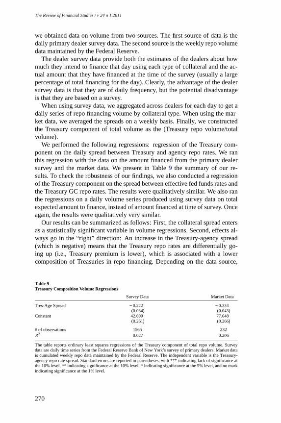
3.4.3 Volume analysis. In this section, we provide some evidence on thelink between repo volumes and repo rates. In order to perform this analysis,

269


we obtained data on volume from two sources. The first source of data is thedaily primary dealer survey data. The second source is the weekly repo volumedata maintained by the Federal Reserve.

The dealer survey data provide both the estimates of the dealers about howmuch they intend to finance that day using each type of collateral and the ac-tual amount that they have financed at the time of the survey (usually a largepercentage of total financing for the day). Clearly, the advantage of the dealersurvey data is that they are of daily frequency, but the potential disadvantageis that they are based on a survey.

When using survey data, we aggregated across dealers for each day to get adaily series of repo financing volume by collateral type. When using the mar-ket data, we averaged the spreads on a weekly basis. Finally, we constructedthe Treasury component of total volume as the (Treasury repo volume/totalvolume).

We performed the following regressions: regression of the Treasury com-ponent on the daily spread between Treasury and agency repo rates. We ranthis regression with the data on the amount financed from the primary dealersurvey and the market data. We present in Table9 the summary of our re-sults. To check the robustness of our findings, we also conducted a regressionof the Treasury component on the spread between effective fed funds rates andthe Treasury GC repo rates. The results were qualitatively similar. We also ranthe regressions on a daily volume series produced using survey data on totalexpected amount to finance, instead of amount financed at time of survey. Onceagain, the results were qualitatively very similar.

Our results can be summarized as follows: First, the collateral spread entersas a statistically significant variable in volume regressions. Second, effects al-ways go in the “right” direction: An increase in the Treasury-agency spread(which is negative) means that the Treasury repo rates are differentially go-ing up (i.e., Treasury premium is lower), which is associated with a lowercomposition of Treasuries in repo financing. Depending on the data source,

Table 9Treasury Composition Volume Regressions

Survey Data MarketData

Tres-Age Spread −0.222 −0.334(0.034) (0.043)

Constant 42.690 77.648(0.261) (0.266)

# of observations 1565 232R2 0.027 0.206

The table reports ordinary least squares regressions of the Treasury component of total repo volume. Surveydata are daily time series from the Federal Reserve Bank of New York’s survey of primary dealers. Market datais cumulated weekly repo data maintained by the Federal Reserve. The independent variable is the Treasury-agency repo rate spread. Standard errors are reported in parentheses, with *** indicating lack of significance atthe 10% level, ** indicating significance at the 10% level, * indicating significance at the 5% level, and no markindicating significance at the 1% level.

270


a one basis point increase in the Treasury-agency spread is associated with a0.22% or 0.33% decrease in the composition of Treasuries in repo financing.Finally, an analysis focusing around quarter-end dates finds Treasury compo-sition almost universally moving in the predicted directions.

4. Impact of Collateral Values on Asset Prices

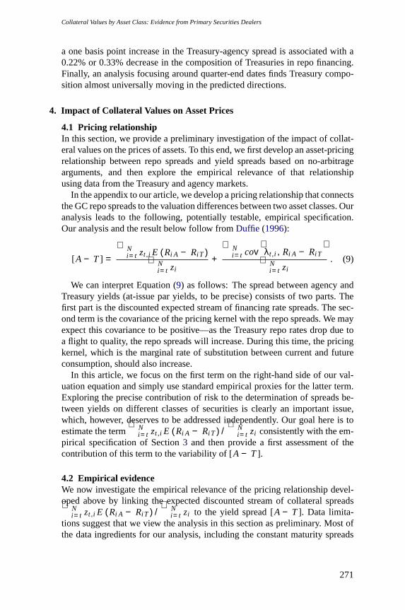
4.1 Pricing relationshipIn this section, we provide a preliminary investigation of the impact of collat-eral values on the prices of assets. To this end, we first develop an asset-pricingrelationship between repo spreads and yield spreads based on no-arbitragearguments, and then explore the empirical relevance of that relationshipusing data from the Treasury and agency markets.

In the appendix to our article, we develop a pricing relationship that connectsthe GC repo spreads to the valuation differences between two asset classes. Ouranalysis leads to the following, potentially testable, empirical specification.Our analysis and the result below follow fromDuffie (1996):

[ A− T ] =

∑Ni=t zt,i E (Ri A − RiT )

∑Ni=t zi

+

∑Ni=t cov

(λt,i , Ri A − RiT

)

∑Ni=t zi

. (9)

We can interpret Equation (9) as follows: The spread between agency andTreasury yields (at-issue par yields, to be precise) consists of two parts. Thefirst part is the discounted expected stream of financing rate spreads. The sec-ond term is the covariance of the pricing kernel with the repo spreads. We mayexpect this covariance to be positive—as the Treasury repo rates drop due toa flight to quality, the repo spreads will increase. During this time, the pricingkernel, which is the marginal rate of substitution between current and futureconsumption, should also increase.

In this article, we focus on the first term on the right-hand side of our val-uation equation and simply use standard empirical proxies for the latter term.Exploring the precise contribution of risk to the determination of spreads be-tween yields on different classes of securities is clearly an important issue,which, however, deserves to be addressed independently. Our goal here is toestimate the term

∑Ni=t zt,i E (Ri A − RiT ) /

∑Ni=t zi consistently with the em-

pirical specification of Section3 and then provide a first assessment of thecontribution of this term to the variability of[ A− T ].

4.2 Empirical evidenceWe now investigate the empirical relevance of the pricing relationship devel-oped above by linking the expected discounted stream of collateral spreads∑N

i=t zt,i E (Ri A − RiT ) /∑N

i=t zi to the yield spread[ A− T ]. Data limita-tions suggest that we view the analysis in this section as preliminary. Most ofthe data ingredients for our analysis, including the constant maturity spreads

271


A− T , the zero-coupon discount factorszi , and, naturally, the expected col-lateral spreadsE (Ri A − RiT ), are constructed under specific empirical as-sumptions. Despite these limitations, we are encouraged by the finding thatcollateral spreads contribute a significant fraction of the variability of short-term(three- and six-month) pricing spreads. By contrast, we find that the contribu-tion of collateral spreads to the variability of pricing spreads at one-year andlonger horizons is small.

The key step needed to estimate the empirical equivalent of Equation (9) isthe calculation ofE (Ri A − RiT ) for all i = t, . . . , N and allt . To this end, foreacht (that is, for each observation in our sample), we used the stochastic pro-cess estimated in Section3 and simulated it forward by Monte Carlo, startingfrom the initial valueRt A − RtT for eacht and computing the sample meanacross paths for eachi . All the sample means are then discounted to the presentusing the zero-coupon discountszi and summed up. For further reference, wedenote the estimated first term of Equation (9) asxt .

As for the other terms in the regression of Equation (9), the discount fac-tors themselves are the Nelson-Siegel-Svensson discount rates estimated by theBoard of Governors of the Federal Reserve; the dependent variableA−T is thespread between the constant-maturity agency rate (provided by Fannie Mae)and the constant-maturity Treasury rate (provided by the Board of Governorsof the Federal Reserve); and the empirical proxies for the risk term∑N

i=t cov(λt,i ,Ri A−RiT )∑Ni=t zi

are the conditional realized volatility, as a risk proxy,

and the average daily bid-ask spreads between 8:00 and 9:00 a.m. for the on-the-run two-year note, which we use as a proxy for the liquidity premium. Wedenote the risk proxy asRPt and the liquidity factor asLt .

The arbitrage arguments are derived assuming that we are long in agencyand short in Treasury so thatA − T always stays positive. In the empiricalwork, we have used the spreadsT − A, but the resulting signs are consistentwith the predictions of the theory. The regression equation that we estimate isspecified below, withxt simulated with respect to theT − A spread:

[Tt − At ] = a0+ a1xt + a2RPt + a3Lt + εt . (10)

The constant terma0 captures the non-time-varying spreads betweenTreasury and agency securities that we do not explicitly model. They mayinclude possible tax effects: Treasury securities are tax exempt at state andcity levels, whereas agency securities are taxable at all levels. The error termεt is assumed to be white noise. We estimate this equation for fixed matu-rity dates, and the results of regressions of Equation (10) are reported inTable10 for six different terms: three and six months, and one, two, five, andten years. We report results for two different sample lengths, with the length ofthe shorter sample determined by the availability of bid-ask spread data fromBrokerTec.

272


Table 10Pricing Spreads Regressions

3 month spread 6 monthspread

Full sample Jan. 1, 2001 – Feb. 3,2006 Full sample Jan. 1, 2001 – Feb. 3,2006

Collateral 20.08 9.97 11.60 11.54 5.91 20.18 12.16 11.15 11.05 8.15value (1.06) (0.88) (0.76) (0.77) (0.66) (1.46) (1.27) (1.00) (1.01) (0.95)

Conditional −2.57 −2.15 −2.78 −1.44volatility (0.08) (0.09) (0.11) (0.11)

Tres. bid-ask −0.16∗∗∗ 0.14∗∗∗ −0.19∗∗∗ −0.02∗∗∗

spread (0.21) (0.18) (0.17) (0.15)Constant 84.83 44.16 45.52 45.17 24.15 88.57 57.56 45.92 45.39 35.21

(5.60) (4.52) (4.00) (4.02) (3.37) (7.63) (6.57) (5.24) (5.26) (4.90)# observations 1548 1526 1243 1243 1221 1548 1526 1243 1243 1221R2 0.188 0.520 0.157 0.158 0.447 0.111 0.374 0.091 0.092 0.220

1 year spread 2 yearspread

Full sample Jan. 1, 2001 – Feb. 3, 2006 Full sample Jan. 1, 2001 – Feb. 3,2006

Collateral 46.04∗ 40.79 28.76 28.25 28.82 33.15 34.42 21.01 19.23 20.14value (3.89) (3.76) (2.89) (2.90) (2.84) (4.91) (4.89) (3.71) (3.70) (3.45)

Conditional −2.27 −0.51∗ −0.13∗ −1.75volatility (0.19) (0.16) (0.06) (0.20)

Tres. bid-ask −0.46∗∗ −0.26∗∗∗ −0.85 −0.66spread (0.25) (0.25) (0.18) (0.17)

Constant 218.24 201.77 133.82 131.22136.75 146.17 153.50 86.52 77.29 86.54(20.31) (19.55) (15.06) (15.11) (14.76) (25.60) (25.48) (19.33) (19.25) (17.95)

# observations 1548 1526 1243 1243 1221 1546 1524 1243 1243 1221R2 0.083 0.165 0.074 0.076 0.092 0.029 0.035 0.025 0.043 0.105

5 year spread 10 yearspread

Full sample Jan. 1, 2001 – Feb. 3, 2006 Full sample Jan. 1, 2001 – Feb. 3,2006

Collateral 78.06 79.16 15.00∗∗∗ 10.76∗∗∗ 15.78∗∗∗ 80.63 69.32∗ −26.19∗∗∗ −31.24∗∗∗ −38.73∗∗∗

value (13.73) (13.54) (10.37) (10.23) (9.49) (27.84) (27.16) (20.74) (20.59) (19.58)Conditional −0.47 −1.48 −1.28 −2.44

volatility (0.08) (0.17) (0.12) (0.22)Tres. bid-ask −1.46 −1.17 −1.43 −1.25

spread (0.23) (0.22) (0.30) (0.29)Constant 361.48 369.26 38.64∗∗∗ 16.72∗∗∗ 47.37∗∗∗ 358.82∗ 304.80∗ −189.77∗∗ −215.89∗ −247.98∗∗∗

(71.47) (70.48) (53.94) (53.24) (49.39) (144.84) (141.27) (107.86) (107.07) (101.84)# observations 1546 1524 1243 1243 1221 1546 1524 1243 1243 1221R2 0.021 0.042 0.002 0.033 0.088 0.005 0.073 0.001 0.019 0.011

The table reports ordinary least squares regressions of constant maturity spreads between yields on Treasury andagency securities, for each term indicated in the table. The independent variables are the discounted stream ofcollateral values constructed as described in the text and normalized by the sum of the zero-coupon-based dis-count rates; the one-month moving average of conditional volatility, which is used as a proxy for risk conditions;and the average (linearly detrended) daily bid-ask spreads between 8:00 and 9:00 a.m. for the on-the-run two-year note, which is used as a proxy for liquidity conditions. Standard errors are reported in parentheses, with*** indicating lack of significance at the 10% level, ** indicating significance at the 10% level, * indicatingsignificance at the 5% level, and no mark indicating significance at the 1% level.

The main lesson revealed from our regressions is that collateral values havesignificant explanatory power for the short-term Treasury-agency spread. Thecoefficients for the discounted streams of collateral values are highly signifi-cant for almost all specifications (their absolute values depend on the time units)and enter with the expected positive sign. Since both the collateral spreadsand yield spreads are negative in sign, an increase in the variables represents a

273


decrease in the spreads; thus, a decrease in collateral spreads is associated witha decrease in yield spreads. However, a more useful metric of this contributionis the fraction of explained variance of the left-hand-side variable, which is19%, 11%, and 8%, respectively, at the three-, six-, and twelve-month ma-turities. The fraction of explained variance falls sharply beyond the one-yearmaturity, confirming previous evidence of sharp structural differences betweenmoney markets and longer-term markets.

As shown in Table10, the realized conditional volatility as a proxy measurefor risk in the regression is highly significant in all specifications and helpsexplain a good portion of the variance.19 Additionally, the risk proxy enterswith the anticipated negative sign (a higher realized conditional volatility, in-dicating a period of heightened risk, is associated with flight-to-quality effectsand thus an increase in the spreadT − A). In effect, the significance of therisk proxy in our regressions is suggestive that we have used an effective proxyfor the risk term in our regression of cross-security bond yield spreads. Whilethe inclusion of the risk proxy does somewhat reduce the magnitude of the es-timated coefficients for the collateral values, the main results are qualitativelyunchanged. The coefficients for the collateral values remain positive and highlystatistically significant, and our simple model can explain 52%, 37%, and 17%of the variance of the dependent variable for the three-, six-, and twelve-monthterms, respectively.

Finally, we included in our regressions measures of liquidity conditions,namely, average bid-ask spreads for the two-year on-the-run Treasuries be-tween 8:00 and 9:00 a.m. (the same time interval over which our repo ratesare sampled). Results of these regressions are also reported in Table10.20 Wefound our measures of liquidity to enter in the regressions with the anticipatednegative sign (a larger spread, indicating tighter liquidity conditions, is asso-ciated with flight-to-quality effects, hence an increase in the spreadT − A),although it is mostly statistically insignificant. Ultimately, the contribution ofour liquidity proxy to explaining the variability of the pricing spreads is verysmall, leaving the estimated coefficients for the collateral values essentiallyunchanged.

Overall, our analysis in this section suggests that in conjunction withstandard measures of risk and liquidity, collateral values can help explain asignificant fraction of the variability of pricing spreads. It is encouraging thatcollateral values explain up to a fifth of the variability of these spreads forshort-term instruments, suggesting this as a promising avenue for furtherinvestigation.

19 The results of the regressions are robust to using other constructed measures of conditional volatility to proxyfor risk. SeeAndersen, Bollerslev, Diebold, and Labys(2003) for a formal treatment of realized volatility.

20 The table reports results of regressions in which bid-ask spreads are linearly detrended, to account for the cleardownward trend in both level and volatility of the bid-ask spreads during the sample, which clearly reflectsthe increased volume of trade on BrokerTec during the period. However, results using undetrended series werequalitatively similar.

274


5. Concluding Remarks

In this article, we have used a novel set of data on early morning repurchaseagreements by primary securities dealers to document a number of featureson the longitudinal and cross-security-class behavior of financing ratesagainst GC.

One of our contributions is to substantiate the widely held—yet undoc-umented—view that three main classes of securities (Treasury securities, secu-rities issued by government-sponsored agencies, and mortgage-backedsecurities) can be ranked in terms of their respective collateral values in theGC market: Holders of Treasury securities enjoy a considerable advantage inthat they can borrow at considerably favorable rates relative to holders of secu-rities issued by government-sponsored agencies and mortgage-backed securi-ties. This advantage (which we quantify as an average unconditional spread of5–6 basis points) displays significant temporal variation, and is especially largeat times of predictable liquidity needs (such as quarter-ends and other specialdays). At these times, Treasury collateral values rise sharply, consistent withsafe-haven effects in favor of Treasury securities.

Our analysis also allows us to measure the collateral rents earned by se-curities’ owners as the spread between unsecured and secured loans and todocument features of the time variation of these rents. We document the sur-prising fact that rates on repos using agency and mortgage-backed securities ascollateral are not meaningfully different from unsecured rates, suggesting thatposting of agency and mortgage-backed securities essentially enables ownersof these securities to obtain (or expand) access to the funding market, althoughit does not generate any significant price advantage.

Finally, we link collateral values to asset prices in a simple no-arbitrageframework, showing that variations in collateral values should explain a sig-nificant fraction of changes in the prices of the underlying securities. We ver-ify empirically that this conjecture holds true for pricing of short-term (moneymarket) securities but not for the pricing of medium-term and long-termsecurities.

AppendixTo develop the needed pricing relationship, we make the following simplifying assumptions. First,we assume that Treasury and agency par bonds are issued in frictionless markets at the same time.We also assume all coupon payment dates to be the same for both types of security, and ignore anyspread difference between repo and reverse repo agreements. Finally, we assume the cash flowsfor both types of securities to be free of default risk.

These assumptions may appear to be rather strong, but they allow us to derive a tractabletheoretical link between the yield spreads of agency and Treasury securities, and their financingspreads. In addition, we are able to use the derived theoretical link to obtain empirically testableimplications.

With these assumptions in place, we consider the following portfolio strategy. Sell an agencypar bond with a coupon ofA and go long in a Treasury par bond with a coupon ofT . Both thelong position in the Treasury security and the short position in the agency security are implemented

275


using GC repo agreements that are renewed every day: The long Treasury position is financed bypaying the repo rate in the GC repo market for Treasury, while the proceeds associated with theshort sale of the agency security earn the repo rate in the GC repo market for agency debt. Note thaton each date, the portfolio earns (on an accrual basis) the amountA− T , which is the differencebetween the agency coupon rate and the Treasury coupon rate. (In practice, we expectA−T > 0 tocompensate for the fact that the Treasury security has a “safe haven” premium built into it, but thisinequality is not needed for our pricing relationship.) Let this position be carried until maturity, atwhich point it is unwound.

The above-described position leads to the following valuation equation:

[ A− T ]N∑

i=t

zi = PV

N∑

i=t

(Ri A − RiT )

, (11)

where thezi are the zero-coupon discount factors andRi A and RiT are the overnight repo ratesagainst agency and Treasury collateral, respectively.

Note that since we assumed the securities to have been issued at par, thenA andT can beinterpreted as the respective coupons and at-issue par yields. Equation (11) then states that thepresent value of par yield spreads is simply the present value of repo spreads. In Equation (11), theconstant-maturity Treasury and agency yields can be interpreted as yields on “new issue” bonds.21

Note that the left-hand side of the pricing relation (11) is the discounted present value ofthe differential cash flow rights between Treasury and agency security. The right-hand side isthe present value of the differential collateral rights. In equilibrium, in the absence of default,liquidity, and tax differences, they must be equal: In other words, differences in valuation arisingfrom differential cash flow rights can be fully explained by the differences in collateral rights. Inthe real world, such differences may also be driven by liquidity differences.

The pricing relation (11) can then be applied over time by recognizing that it should applyto the par yield spreads on each date. Since par yields in the Treasury and agency securities areestimated every day, we can then apply our valuation equation on the par yield spreads in themarket.

To this end, let us explore the right-hand side of the valuation equation in greater detail byrewriting (11) as

PV

N∑

i=t

(Ri A − RiT )

= E

N∑

i=t

λt,i (Ri A − RiT )

, (12)

where the time-varying pricing kernelλt,i covaries with the repo spreads. We can then expand thepricing relationship and exploit the fact that

E[λt,i

]= zt,i , (13)

21 Several points are worthy of note. First, we assume that the agency debt securities are free of default risk. Thismay be called into question, as they are not backed by the full faith and credit of the United States government.At the time of writing this article, it was a widely held belief among the market participants that the GovernmentSponsored Enterprises would not be allowed to fail. In fact, in September 2008, the Treasury announced a con-servatorship program and essentially took Fannie Mae and Freddie Mac under its wings. Second, the assumptionthat repo and reverse repo transactions are carried until maturity is a conceptual device, which allows us to geta tractable specification. Finally, it should be noted that in Equation (11), a long position is held in agenciesand a short position in Treasuries. Short positions are established in “specials” markets, but for empirical imple-mentation, we will be using the GC rates. This actually biases our model toward rejection, as special rates aremuch lower than GC rates, and financing spreads using the Treasury special rates are likely to exhibit greaterco-movements with yield spreads.

276


which states that the expected value of the pricing kernel is the price of a zero-coupon bond at thetime expectation is taken. Plugging this into the valuation equation and simplifying, we get

PV

N∑

i=t

(Ri A − RiT )

=N∑

i=t

zt,i E (Ri A − RiT )+N∑

i=t

cov(λt,i , Ri A − RiT

). (14)

We can further simplify as follows:

[ A− T ]N∑

i=t

zi =N∑

i=t

zt,i E (Ri A − RiT )+N∑

i=t

cov(λt,i , Ri A − RiT

), (15)

or, rearranging,

[ A− T ] =

∑Ni=t zt,i E (Ri A − RiT )

∑Ni=t zi

+

∑Ni=t cov

(λt,i , Ri A − RiT

)

∑Ni=t zi

. (16)

ReferencesAndersen, T., T. Bollerslev, F. Diebold, and P. Labys. 2003. Modeling and Forecasting Realized Volatility.Econometrica71:579–625.

Bindseil, U., K. Nyborg, and I. Strebulaev. 2002. Bidding and Performance in Repo Auctions: Evidence fromECB Open Market Operations. ECD Working Paper 157.

. 2009. Repo Auctions and the Market for Liquidity.Journal of Money, Credit, and Banking41:1391–421.

Brunnermeir, M. K., and L. H. Pedersen. 2009. Market Liquidity and Funding Liquidity.Review of FinancialStudies22:2201–38.

Cornell, B., and A. C. Shapiro. 1989. The Mispricing of U.S. Treasury Bonds: A Case Study.Review of FinancialStudies2:297–310.

Duffie, D. 1996. Special Repo Rates.Journal of Finance51:493–526.

Eraker, B., M. Johannes, and N. Polson. 2003. The Impact of Jumps in Volatility and Returns.Journal of Finance58:1269–300.

Fleming, M., and K. Garbade. 2002. When the Back Office Moved to the Front Burner: Settlement Fails in theTreasury Market after 9/11.Economic Policy Review8(2):35–57.

. 2003. The Repurchase Agreement Refined: GCF Repo.Current Issues in Economics and Finance9(2):1–7.

Garleanu, N., and L. H. Pedersen. 2009. Margin-based Asset Pricing and Deviations from the Law of One Price.Working Paper, New York University.

Geanakaplos, J. 1997. Promises, Promises. In W. B. Arthur, S. Durlauf, and D. Lane (eds.),The Economy as anEvolving Complex System II, pp. 285–320. Reading, MA: Addison-Wesley.

. 2003. Liquidity, Default, and Crashes: Endogenous Contracts in General Equilibrium. InM. Dewatripont, L. P. Hansen, and S. J. Turnovsky (eds.),Advances in Economics and Econometrics: The-ory and Applications, Eighth World Conference, Vol. 2, Ch. 5, pp. 170–205. Cambridge: Econometric SocietyMonographs.

. 2009. The Leverage Cycle. Cowles Foundation Discussion Paper 1715.

Gurkaynak, R. S., B. Sack, and J. H. Wright. 2007. The U.S. Treasury Yield Curve: 1961 to the Present.Journalof Monetary Economics54:2291–304.

277


Herring, R., and T. Schuermann. 2005. Capital Regulation for Position Risk in Banks, Securities Firms, andInsurance Companies. In H. S. Scott (ed.),Capital Adequacy Beyond Basel: Banking, Securities, and Insurance,Ch. 1, pp. 15–86. New York: Oxford University Press.

Heston, S. L. 1993. A Closed-form Solution for Options with Stochastic Volatility with Applications to Bondand Currency Options.Review of Financial Studies6:327–43.

Jacquier, E., N. Polson, and P. Rossi. 1994. Bayesian Analysis of Stochastic Volatility Models.Journal ofEconomics and Business Statistics12:371–89.

Johannes, M., and N. Polson. 2006. MCMC Methods for Continuous-time Financial Econometrics. InY. Ait-Sahalia and L.-P. Hansen (eds.),Handbook of Financial Econometrics, Vol. 2, Ch. 13. Oxford: Else-vier.

Jordan, B. D., and S. D. Jordan. 1997. Special Repo Rates: An Empirical Analysis.Journal of Finance52:2051–72.

Krishnamurthy, A. 2002. The Bond/Old-bond Spread.Journal of Financial Economics66:463–506.

Longstaff, F. A. 2004. The Flight-to-liquidity Premium in U.S. Treasury Bond Prices.Journal of Business77:511–26.

Markets Group of the Federal Reserve Bank of New York. 2009. Domestic Open Market Operations During2008. Technical Report.

Musto, D. K. 1997. Portfolio Disclosures and Year-end Price Shifts.Journal of Finance52:1563–88.

Securities Industry and Financial Markets Association. 2009. Research Statistical Tables: “U.S. Bond MarketOutstanding” and “U.S. Primary Dealer Financing”. Technical Report.

Staff Publications Committee. 2009. Statistical Supplement to the Federal Reserve Bulletin. Technical Report,Board of Governors of the Federal Reserve Bank.

Sundaresan, S. 1994. An Empirical Analysis of U.S. Treasury Auctions: Implications for Auction and TermStructure Theories.Journal of Fixed Income4(2):35–50.

Sundaresan, S., and Z. Wang. 2009. Y2K Options and Liquidity Premium in Treasury Markets.Review of Fi-nancial Studies22:1021–56.

Treasury Market Practices Group. 2009. Treasury Market Best Practices. Technical Report.

278

Copyright of Review of Financial Studies is the property of Society for Financial Studies and its content may

not be copied or emailed to multiple sites or posted to a listserv without the copyright holder's express written

permission. However, users may print, download, or email articles for individual use.

Collateral Values by Asset Class: Evidence from Primary ... · Collateral Values by Asset Class:...

Documents

Transcript of Collateral Values by Asset Class: Evidence from Primary ... · Collateral Values by Asset Class:...