COGNITIVE AND NEURAL SYSTEMS, BOSTON UNIVERSITY Boston, Massachusetts Madhusudana Shashanka...
66
COGNITIVE AND NEURAL SYSTEMS, BOSTON UNIVERSITY Boston, Massachusetts Madhusudana Shashanka [email protected] 17 August 2007 Dissertation Defense Latent Variable Framework for Modeling and Separating Single-Channel Acoustic Sources Committee Chair: Prof. Daniel Bullock Readers: Prof. Barbara Shinn-Cunningham Dr. Paris Smaragdis Prof. Frank Guenther Reviewers: Dr. Bhiksha Raj Prof. Eric Schwartz
-
date post
22-Dec-2015 -
Category
Documents
-
view
214 -
download
0
Transcript of COGNITIVE AND NEURAL SYSTEMS, BOSTON UNIVERSITY Boston, Massachusetts Madhusudana Shashanka...
COGNITIVE AND NEURAL SYSTEMS, BOSTON UNIVERSITYBoston, Massachusetts
Madhusudana [email protected]
17 August 2007Dissertation Defense
Latent Variable Framework for Modeling andSeparating Single-Channel Acoustic Sources
CommitteeChair: Prof. Daniel BullockReaders: Prof. Barbara Shinn-Cunningham
Dr. Paris Smaragdis Prof. Frank Guenther
Reviewers: Dr. Bhiksha Raj Prof. Eric Schwartz

2
Outline
• Introduction• Time-Frequency Structure Background• Latent Variable Decomposition:
A Probabilistic Framework Contributions• Sparse Overcomplete Decomposition• Conclusions
3
Introduction
The achievements of the ear are indeed fabulous. While I am writing, my elder son
rattles the fire rake in the stove, the infant babbles contentedly in his baby carriage, the church clock strikes the hour, …
… In the vibrations of air striking my ear, all these sounds are superimposed into a single extremely complex stream of pressure waves. Without doubt the achievements of the ear are greater than those of the eye.
Wolfgang Metzger, in Gesetze des Sehens (1953)
Abridged in English and quoted by Reinier Plomp (2002)
Introduction

4
Cocktail Party Effect
Introduction Cocktail Party Effect
(Cocktail Party by SLAW, Maniscalco Gallery. From slides of Prof. Shinn-Cunningham, ARO 2006)
Colin Cherry (1953)
Our ability to follow one speaker in the presenceof other sounds.
The auditory system separates the input intodistinct auditory objects.
Challenging problem from a computationalperspective.

5
Cocktail Party Effect
• Fundamental questions– How does the brain solve it?– Is it possible to build a machine capable of solving it in a
satisfactory manner?• Need not mimic the brain
• Two cases– Multi-channel (Human auditory system is an example with two
sensors)– Single-Channel
Introduction Cocktail Party Effect

6
Source Separation: Formulation
•
• Given just , how to separate sources ?
• Problem: Indeterminacy – Multiple ways in which
source signals can be reconstructed from the available information
Introduction Source Separation
x(t) =NX
j =1
sj (t)
x(t)
s1(t)
sN (t)
sj (t). . .
. ..
x(t)
sj (t)
7
Source Separation: Approaches
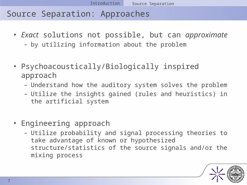
• Exact solutions not possible, but can approximate – by utilizing information about the problem
• Psychoacoustically/Biologically inspired approach – Understand how the auditory system solves the problem– Utilize the insights gained (rules and heuristics) in the artificial
system
• Engineering approach– Utilize probability and signal processing theories to take
advantage of known or hypothesized structure/statistics of the source signals and/or the mixing process
Introduction Source Separation

8
Source Separation: Approaches
• Psychoacoustically inspired approach – Seminal work of Bregman (1990) - Auditory Scene Analysis (ASA)– Computational Auditory Scene Analysis (CASA)– Computational implementations of the views outlined by Bregman
(Rosenthal and Okuno, 1998)– Limitations: reconcile subjective concepts (e.g. “similarity”,
“continuity”) with strictly deterministic computational platforms?– Difficulty incorporating statistical information
• Engineering approach– Most work has focused on multi-channel signals– Blind Source Separation: Beamforming and ICA– Unsuitable for single-channel signals
Introduction Source Separation
9
Source Separation: This Work
• We take a machine learning approach in a supervised setting– Assumption: One or more sources present in the mixture are
“known”– Analyze the sample waveforms of the known sources and extract
characteristics unique to each one– Utilize the learned information for source separation and other
applications
• Focus on developing a probabilistic framework for modeling single-channel sounds– Computational perspective, goal not to explain human auditory
processing– Provide a framework grounded in theory that allows principled
extensions – Aim is not just to build a particular separation system
Introduction Source Separation
10
Outline
• Introduction• Time-Frequency Structure
– We need a representation of audio to proceed
• Latent Variable Decomposition:
A Probabilistic Framework• Sparse Overcomplete Decomposition• Conclusions

11
RepresentationTime-Frequency Structure Audio Representation
FREQ
TIME
Time-domain representation
Sampled waveform: each sample represents the sound pressure level at a particular time instant.
Time-Frequency representation
TF representation shows energy in TF bins explicitly showing the variation along time and frequency.
TIME
AMPL
12
TF RepresentationsTime-Frequency Structure Audio Representation
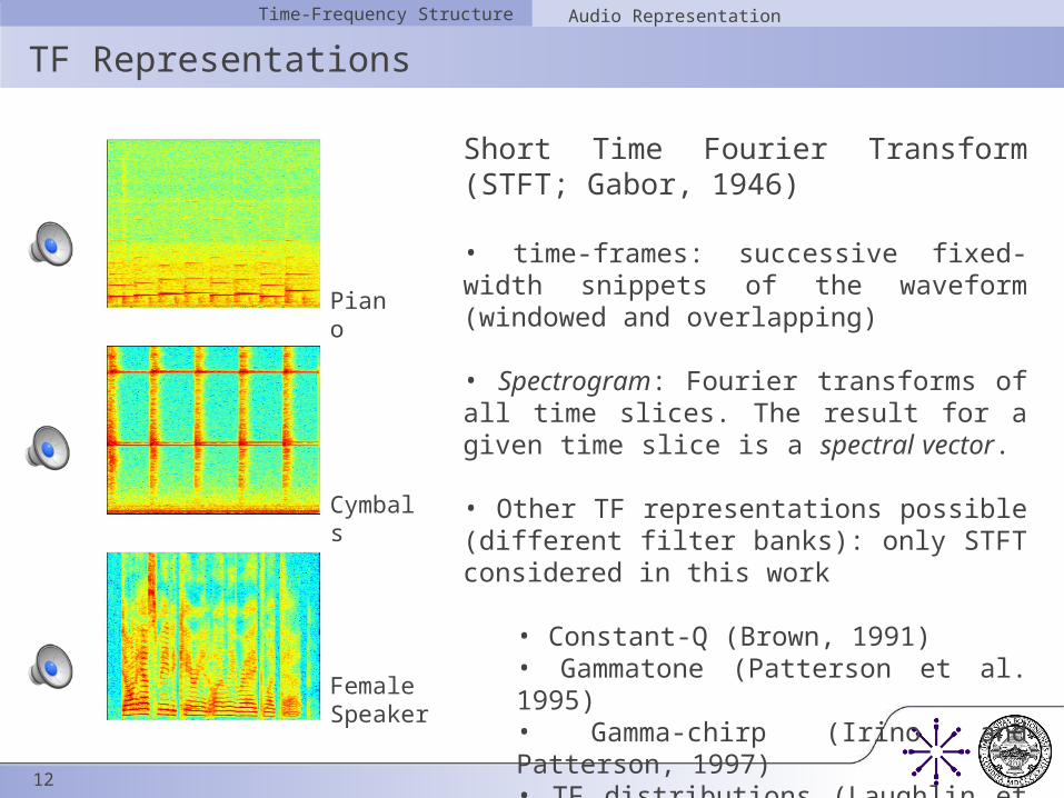
Short Time Fourier Transform (STFT; Gabor, 1946)
• time-frames: successive fixed-width snippets of the waveform (windowed and overlapping)
• Spectrogram: Fourier transforms of all time slices. The result for a given time slice is a spectral vector.
• Other TF representations possible (different filter banks): only STFT considered in this work
• Constant-Q (Brown, 1991)• Gammatone (Patterson et al. 1995)• Gamma-chirp (Irino and Patterson, 1997)• TF distributions (Laughlin et al. 1994)
Piano
Cymbals
Female Speaker
13
Magnitude SpectrogramsTime-Frequency Structure Audio Representation
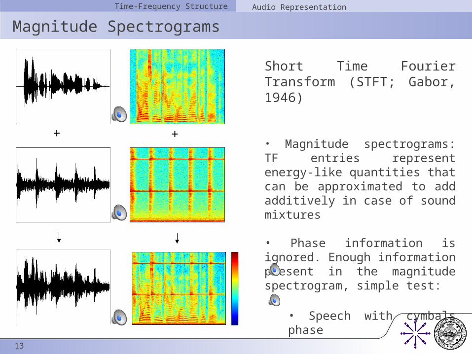
Short Time Fourier Transform (STFT; Gabor, 1946)
• Magnitude spectrograms: TF entries represent energy-like quantities that can be approximated to add additively in case of sound mixtures
• Phase information is ignored. Enough information present in the magnitude spectrogram, simple test:
• Speech with cymbals phase
• Cymbals with piano phase
+ +
14
TF Masks
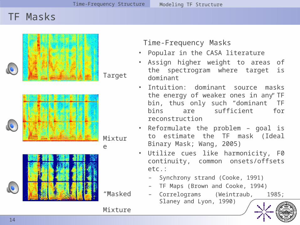
Time-Frequency Masks• Popular in the CASA literature
• Assign higher weight to areas of the spectrogram where target is dominant
• Intuition: dominant source masks the energy of weaker ones in any TF bin, thus only such “dominant” TF bins are sufficient for reconstruction
• Reformulate the problem – goal is to estimate the TF mask (Ideal Binary Mask; Wang, 2005)
• Utilize cues like harmonicity, F0 continuity, common onsets/offsets etc.:
– Synchrony strand (Cooke, 1991) – TF Maps (Brown and Cooke, 1994)– Correlograms (Weintraub, 1985; Slaney
and Lyon, 1990)
Time-Frequency Structure Modeling TF Structure
Target
Mixture
“Masked” Mixture
15
TF Masks
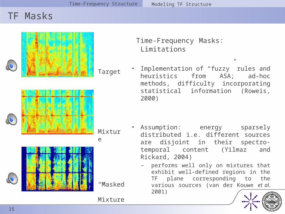
Time-Frequency Masks: Limitations
• Implementation of “fuzzy” rules and heuristics from ASA; ad-hoc methods, difficulty incorporating statistical information (Roweis, 2000)
• Assumption: energy sparsely distributed i.e. different sources are disjoint in their spectro-temporal content (Yilmaz and Rickard, 2004)
– performs well only on mixtures that exhibit well-defined regions in the TF plane corresponding to the various sources (van der Kouwe et al. 2001)
Time-Frequency Structure Modeling TF Structure
Target
Mixture
“Masked” Mixture
16
Basis Decomposition Methods
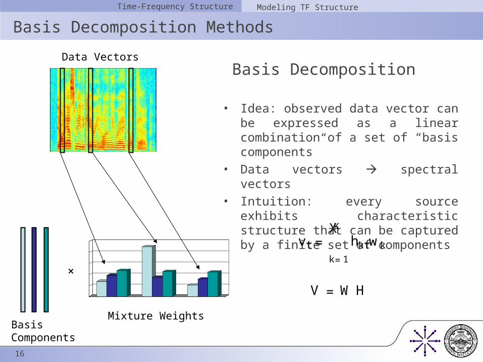
Basis Decomposition
• Idea: observed data vector can be expressed as a linear combination of a set of “basis components”
• Data vectors spectral vectors
• Intuition: every source exhibits characteristic structure that can be captured by a finite set of components
Time-Frequency Structure Modeling TF Structure
Data Vectors
Mixture WeightsBasis Components
vt =KX
k=1
hktwk
V = W H
+
17
Basis Decomposition Methods
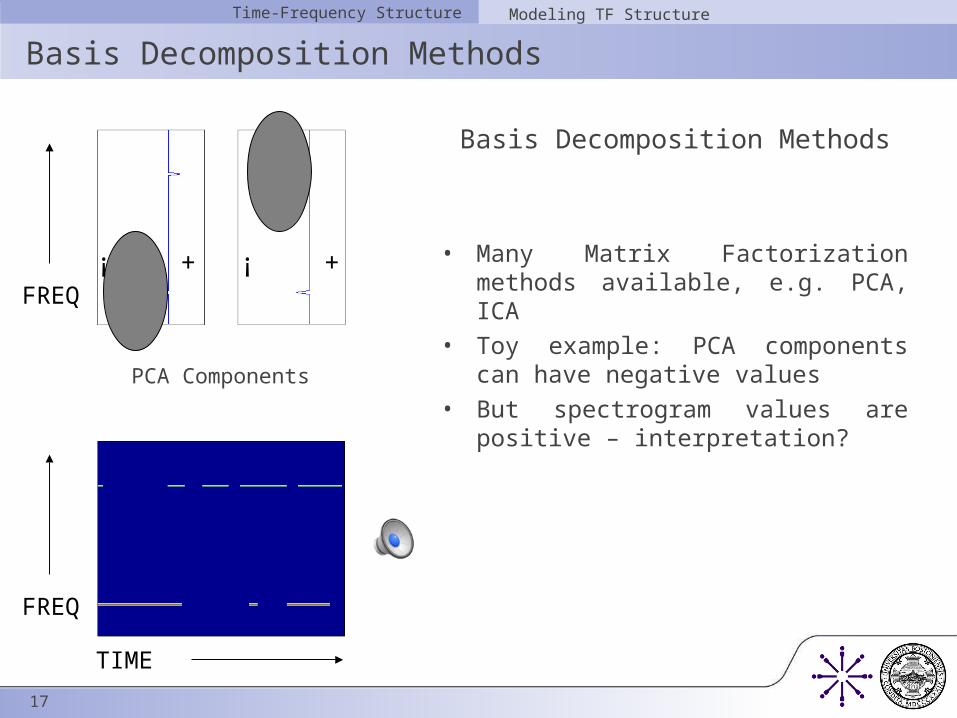
Basis Decomposition Methods
• Many Matrix Factorization methods available, e.g. PCA, ICA
• Toy example: PCA components can have negative values
• But spectrogram values are positive – interpretation?
Time-Frequency Structure Modeling TF Structure
+¡+¡
PCA Components
FREQ
TIME
FREQ
18
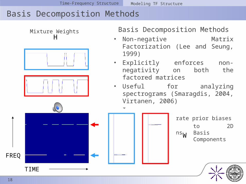
Basis Decomposition Methods
Basis Decomposition Methods• Non-negative Matrix Factorization (Lee
and Seung, 1999)
• Explicitly enforces non-negativity on both the factored matrices
• Useful for analyzing spectrograms (Smaragdis, 2004, Virtanen, 2006)
• Issues– Can’t incorporate prior biases– Restricted to 2D representations
Time-Frequency Structure Modeling TF Structure
W
HMixture Weights
BasisComponents
FREQ
TIME

19
Outline
• Introduction• Time-Frequency Structure• Latent Variable Decomposition: Probabilistic Framework
– Our alternate approach: Latent variable decomposition treating spectrograms as histograms
• Sparse Overcomplete Decomposition• Conclusions
20
Latent Variables
• Widely used in social and behavioral sciences– Traced back to Spearman (1904), factor analytic models for
Intelligence Testing
• Latent Class Models (Lazarsfeld and Henry, 1968)– Principle of local independence (or the common cause criterion)– If a latent variable underlies a number of observed variables, the
observed variables conditioned on the latent variable should be independent
Latent Variable Decomposition Background
21
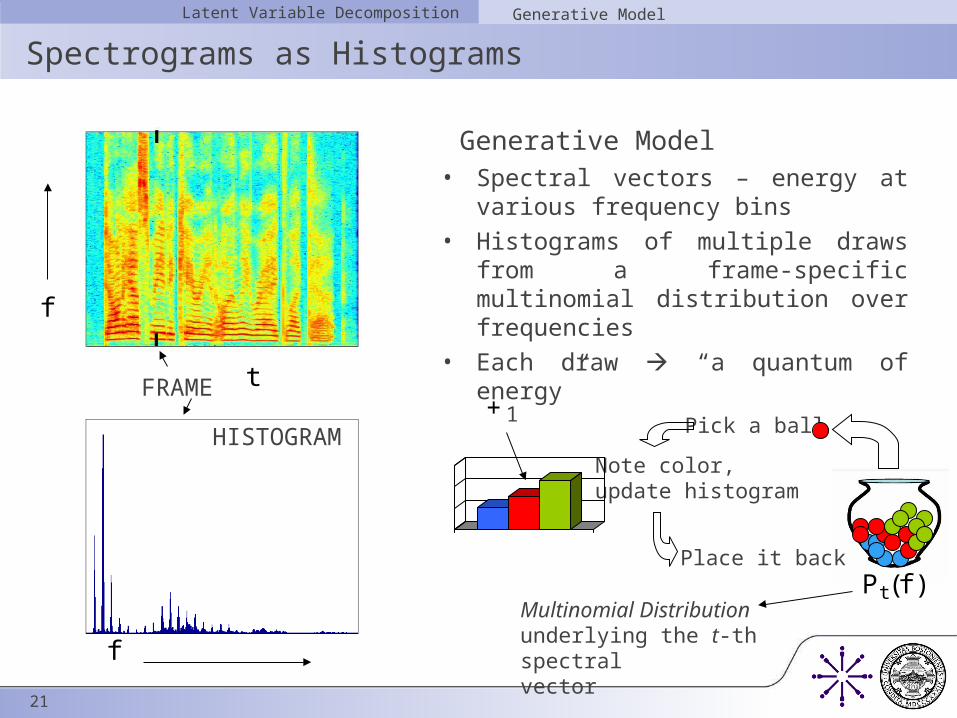
Spectrograms as Histograms
Generative Model• Spectral vectors – energy at various
frequency bins
• Histograms of multiple draws from a frame-specific multinomial distribution over frequencies
• Each draw “a quantum of energy”
Latent Variable Decomposition Generative Model
f
HISTOGRAM
f
FRAME t
HISTOGRAM Pick a ball
Note color,update histogram
+1
Place it back
Multinomial Distributionunderlying the t-th spectralvector
Pt(f )
22
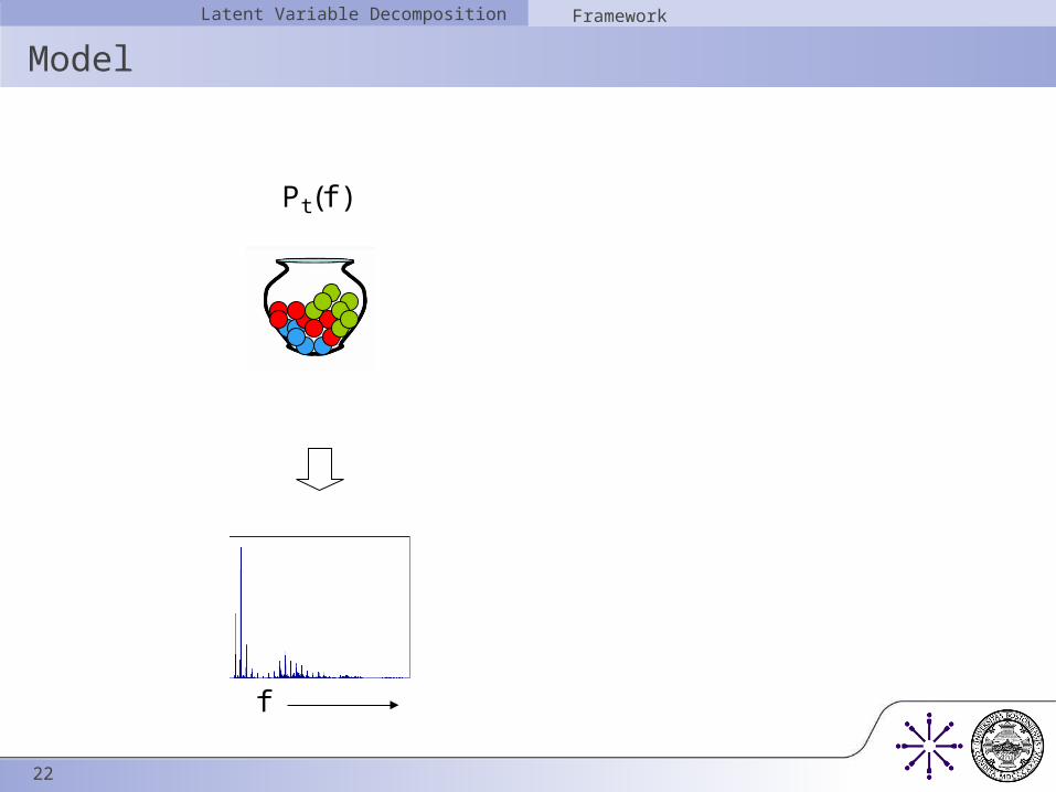
ModelLatent Variable Decomposition Framework
f
Pt(f )

23
ModelLatent Variable Decomposition Framework
f
P (f jz)
Pt(z)
Pt(f ) =X
z
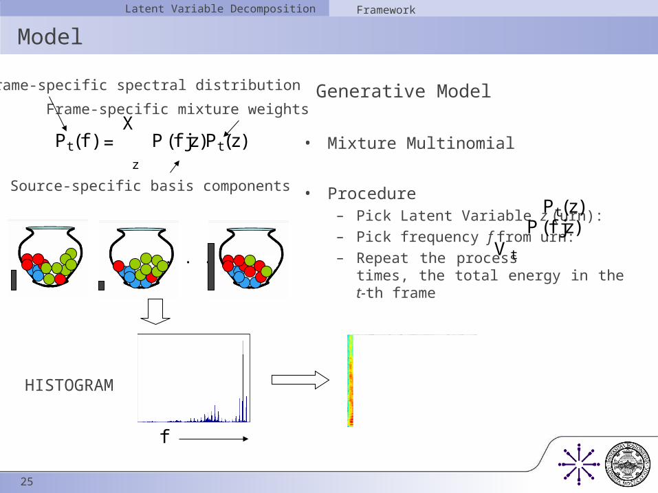
P (f jz)Pt(z)Generative Model
• Mixture Multinomial
• Procedure– Pick Latent Variable z (urn):– Pick frequency f from urn:– Repeat the process times,
the total energy in the t-th frame
Pt(z)P (f jz)
V t

24
Model
Generative Model
• Mixture Multinomial
• Procedure– Pick Latent Variable z (urn):– Pick frequency f from urn:– Repeat the process times, the total
energy in the t-th frame
Latent Variable Decomposition Framework
f
HISTOGRAM
. . .
Pt(z)P (f jz)
V t
Pt(f ) =X
z
P (f jz)Pt(z)
Frame-specific spectral distribution
Frame-specific mixture weights
Source-specific basis components
25
ModelLatent Variable Decomposition Framework
f
HISTOGRAM
. . .
Pt(f ) =X
z
P (f jz)Pt(z)
Frame-specific spectral distribution
Frame-specific mixture weights
Source-specific basis components
Generative Model
• Mixture Multinomial
• Procedure– Pick Latent Variable z (urn):– Pick frequency f from urn:– Repeat the process times, the total
energy in the t-th frame
Pt(z)P (f jz)
V t

26
ModelLatent Variable Decomposition Framework
f
HISTOGRAM
. . .
Pt(f ) =X
z
P (f jz)Pt(z)
Frame-specific spectral distribution
Frame-specific mixture weights
Source-specific basis components
Generative Model
• Mixture Multinomial
• Procedure– Pick Latent Variable z (urn):– Pick frequency f from urn:– Repeat the process times, the total
energy in the t-th frame
Pt(z)P (f jz)
V t

27
ModelLatent Variable Decomposition Framework
f
Pt(f )
P (f jz)
Pt(z)
Pt(f ) =X
z
P (f jz)Pt(z)Generative Model
• Mixture Multinomial
• Procedure– Pick Latent Variable z (urn):– Pick frequency f from urn:– Repeat the process times,
the total energy in the t-th frame
Pt(z)P (f jz)
V t
28
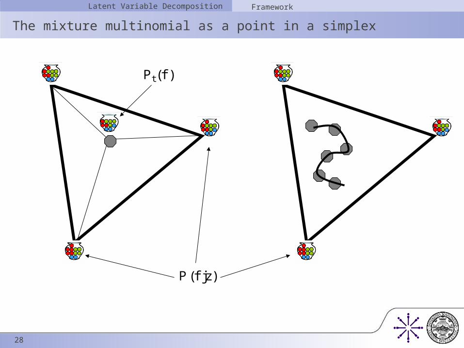
The mixture multinomial as a point in a simplex
Latent Variable Decomposition Framework
P (f jz)
Pt(f )
29
Learning the Model
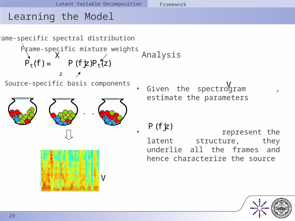
Analysis
• Given the spectrogram , estimate the parameters
• represent the latent structure, they underlie all the frames and hence characterize the source
Latent Variable Decomposition Framework
. . .
Pt(f ) =X
z
P (f jz)Pt(z)
Frame-specific spectral distribution
Frame-specific mixture weights
Source-specific basis components
P (f jz)
V
V
30
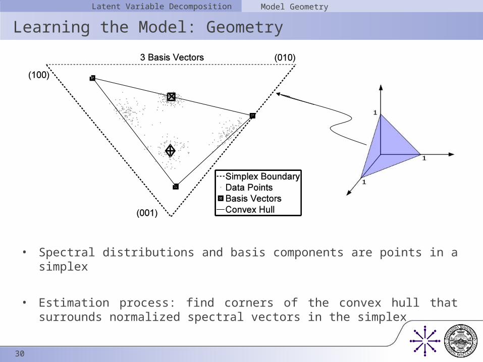
Learning the Model: GeometryLatent Variable Decomposition Model Geometry
• Spectral distributions and basis components are points in a simplex
• Estimation process: find corners of the convex hull that surrounds normalized spectral vectors in the simplex

31
Learning the Model: Parameter Estimation
• Expectation-Maximization Algorithm
Latent Variable Decomposition Framework
Pt(z) =
Pf Vf tPt(zjf )
Pz
Pf Vf tPt(zjf )P (f jz) =
Pt Vf tPt(zjf )
Pf
Pt Vf tPt(zjf )
Pt(zjf ) =Pt(z)P (f jz)
Pz Pt(z)P (f jz)
Vf t Entries of the training spectrogram
32
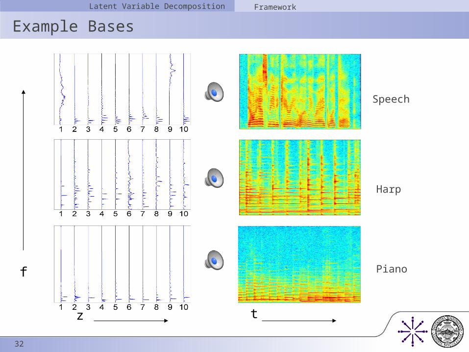
Example Bases Latent Variable Decomposition Framework
f
z t
Speech
Harp
Piano

33
Source Separation Latent Variable Decomposition Source Separation
SpeechHarp

34
Source Separation Latent Variable Decomposition Source Separation
SpeechHarp Mixture
SpeechBases
HarpBases

35
Source SeparationLatent Variable Decomposition Source Separation
• Mixture Spectrogram Model – linear combination of individual sources
Pt(f ) = Pt(s1)P (f js1) +Pt(s2)P (f js2)
Pt(f ) =
Ã
Pt(s1)X
z2f zs1 g
Pt(zjs1)Ps1(f jz)
!
+
Ã
Pt(s2)X
z2f zs2 g
Pt(zjs2)Ps2(f jz)
!

36
Source SeparationLatent Variable Decomposition Source Separation
Pt(s;zjf ) =Pt(s)Pt(zjs)Ps(f jz)
Ps Pt(s)
Pz2f zs g Pt(zjs)Ps(f jz)
Pt(f ;s) = Pt(s)X
z2f zs g
Pt(zjs)Ps(f jz)
• Expectation-Maximization Algorithm
Pt(s) =
Pf Vf t
Pz2f zs g Pt(s;zjf )
Ps
Pf Vf t
Pz2f zs g Pt(s;zjf )
Pt(zjs) =
Pf Vf tPt(s;zjf )
Pz2f zs g
Pf Vf tPt(s;zjf )
Vf t
Entries of themixture spectrogram
37
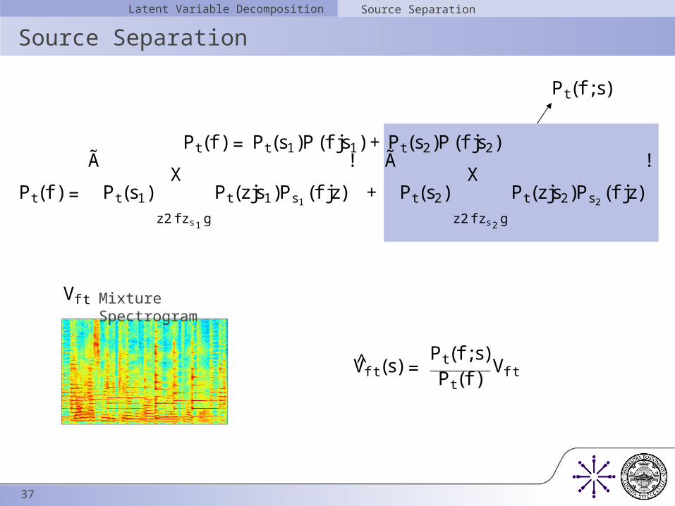
Source SeparationLatent Variable Decomposition Source Separation
Pt(f ) = Pt(s1)P (f js1) +Pt(s2)P (f js2)
Pt(f ) =
Ã
Pt(s1)X
z2f zs1 g
Pt(zjs1)Ps1(f jz)
!
+
Ã
Pt(s2)X
z2f zs2 g
Pt(zjs2)Ps2(f jz)
!
Vf t Mixture Spectrogram
Vf t(s) =Pt(f ;s)Pt(f )
Vf t
Pt(f ;s)

38
Source SeparationLatent Variable Decomposition Source Separation
V©
O
R
Magnitude of the mixture
Phase of the mixture
Mag. of the original signal
Mag. of the reconstruction
g(X ) = 10log10
³ Pf ; t O2
f tPf ; t jO f t ej ©f t ¡ X f t ej ©f t j2
´
Mixture
Reconstructions
SNR Improvements 5.25 dB 5.30 dB
SN R = g(R ) ¡ g(V )
39
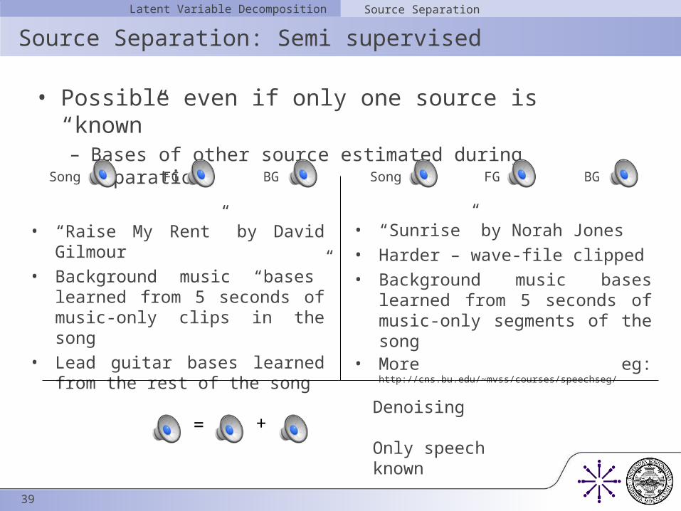
Source Separation: Semi supervisedLatent Variable Decomposition Source Separation
• Possible even if only one source is “known”– Bases of other source estimated during separation
• “Raise My Rent” by David Gilmour
• Background music “bases” learned from 5 seconds of music-only clips in the song
• Lead guitar bases learned from the rest of the song
• “Sunrise” by Norah Jones
• Harder – wave-file clipped
• Background music bases learned from 5 seconds of music-only segments of the song
• More eg: http://cns.bu.edu/~mvss/courses/speechseg/
Song FG BG Song FG BG
= +Denoising
Only speechknown
40
Outline
• Introduction• Time-Frequency Structure• Latent Variable Decomposition: Probabilistic Framework• Sparse Overcomplete Decomposition
– Learning more structure than the dimensionality will allow
• Conclusions
41
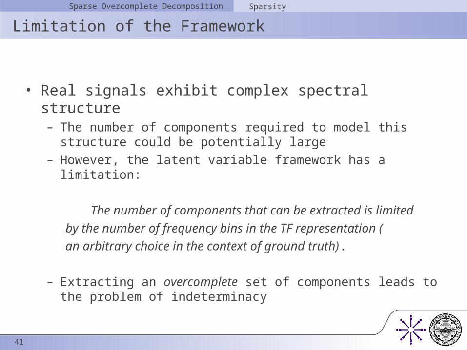
Limitation of the Framework
• Real signals exhibit complex spectral structure – The number of components required to model this structure could
be potentially large– However, the latent variable framework has a limitation:
The number of components that can be extracted is limited
by the number of frequency bins in the TF representation (
an arbitrary choice in the context of ground truth).
– Extracting an overcomplete set of components leads to the problem of indeterminacy
Sparse Overcomplete Decomposition Sparsity
42
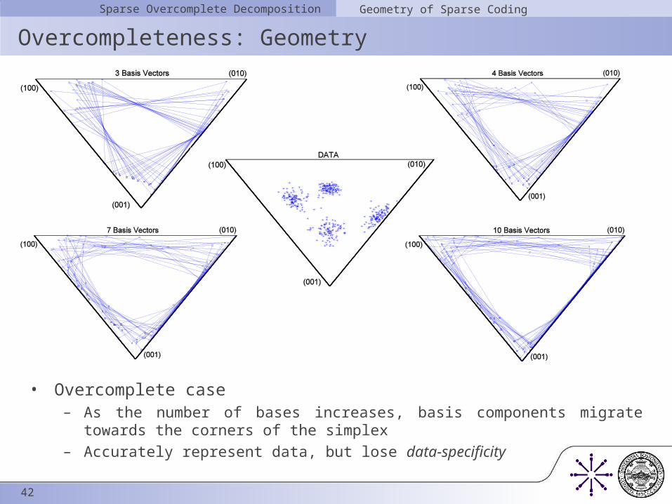
Overcompleteness: GeometrySparse Overcomplete Decomposition Geometry of Sparse Coding
• Overcomplete case– As the number of bases increases, basis components migrate towards the corners
of the simplex– Accurately represent data, but lose data-specificity

43
Indeterminacy in the Overcomplete CaseSparse Overcomplete Decomposition Geometry of Sparse Coding
• Multiple solutions that have zero error indeterminacy

44
Sparse CodingSparse Overcomplete Decomposition Geometry of Sparse Coding
• Restriction use the fewest number of corners – At least three required for accurate representation– The number of possible solutions greatly reduced, but still indeterminate– Instead, we minimize the entropy of mixture weights
ABD, ACE, ACDABE, ABG, ACGACF

45
Sparsity
• Sparsity – originated as a theoretical basis for sensory coding (Kanerva, 1988; Field, 1994; Olshausen and Field, 1996)– Following Attneave (1954), Barlow (1959, 1961) to use
information-theoretic principles to understand perception– Has utility in computational models and engineering methods
• How to measure sparsity?– fewer number of components more sparsity
• Number of non-zero mixture weights i.e. the L0 norm
– L0 hard to optimize; L1 (or L2 in certain cases) used as an approximation
– We use entropy of the mixture weights as the measure
Sparse Overcomplete Decomposition Sparsity
46
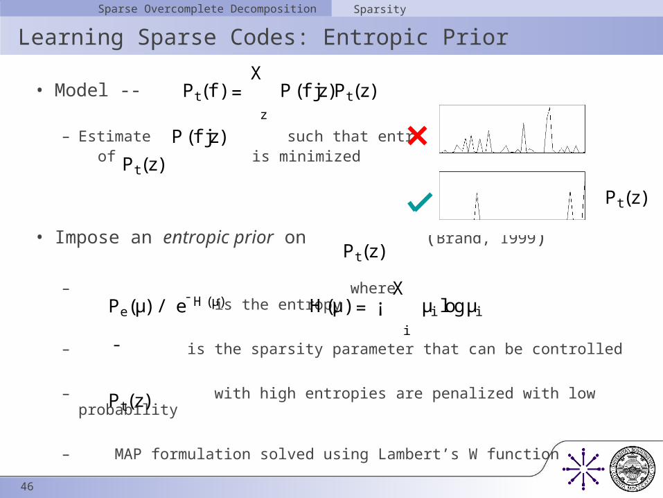
Learning Sparse Codes: Entropic Prior
• Model --
– Estimate such that entropy of is minimized
• Impose an entropic prior on (Brand, 1999)
– where is the entropy
– is the sparsity parameter that can be controlled
– with high entropies are penalized with low probability
– MAP formulation solved using Lambert’s W function
Sparse Overcomplete Decomposition Sparsity
P (f jz)
Pt(z)
Pt(z)
H(µ) = ¡X
i
µi logµi
Pt(z)
Pe(µ) / e H (µ)
Pt(f ) =X
z
P (f jz)Pt(z)
Pt(z)
¯
47
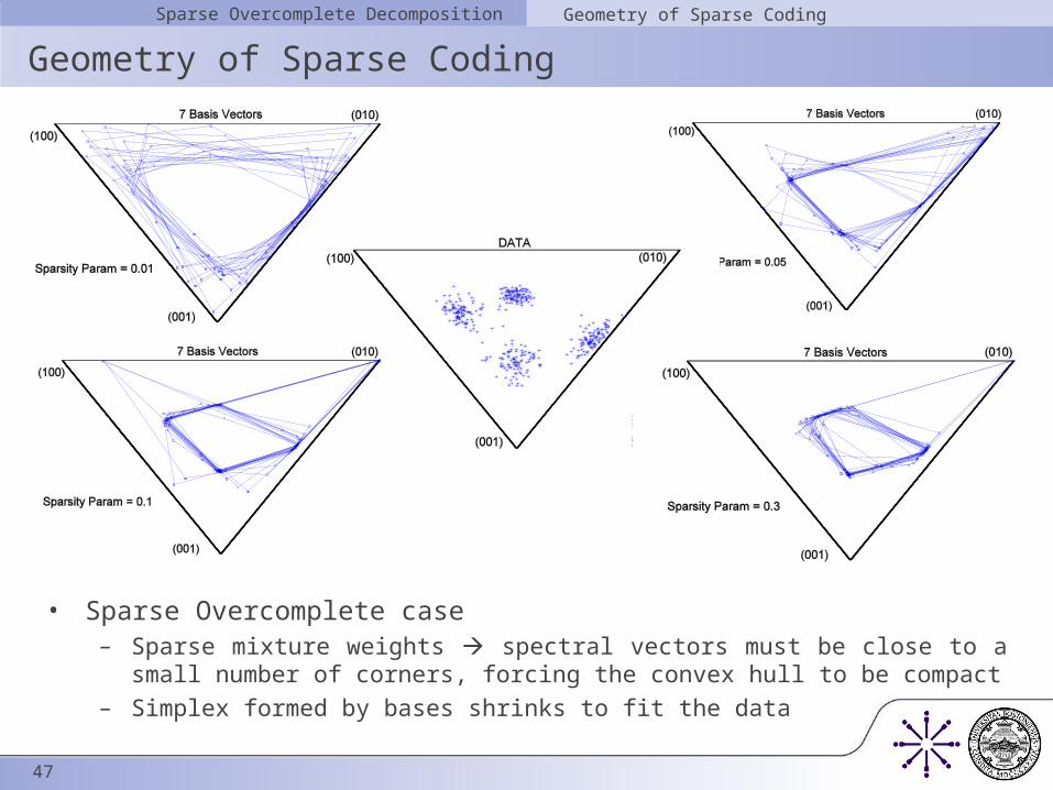
Geometry of Sparse CodingSparse Overcomplete Decomposition Geometry of Sparse Coding
• Sparse Overcomplete case– Sparse mixture weights spectral vectors must be close to a small number of
corners, forcing the convex hull to be compact– Simplex formed by bases shrinks to fit the data

48
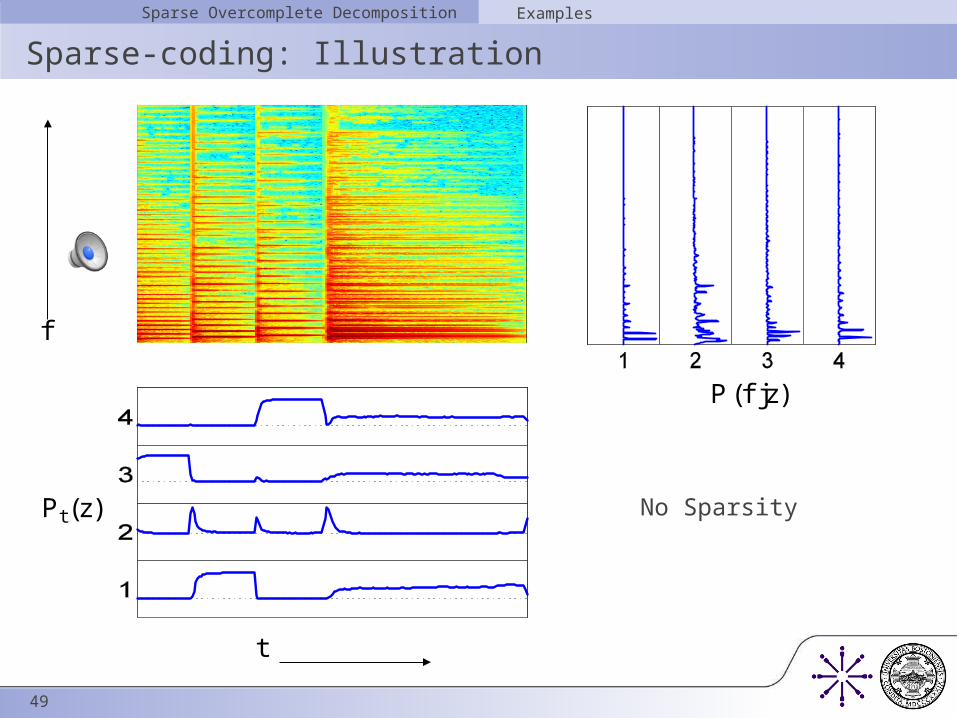
Sparse-coding: IllustrationSparse Overcomplete Decomposition Examples
P (f jz)
Pt(z)
f
t
No Sparsity
49
Sparse-coding: IllustrationSparse Overcomplete Decomposition Examples
P (f jz)
Pt(z)
f
t
No Sparsity

50
Sparse-coding: IllustrationSparse Overcomplete Decomposition Examples
P (f jz)
Pt(z)
f
t
Sparse Mixture Weights
51
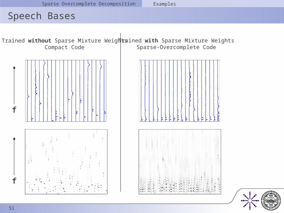
Speech BasesSparse Overcomplete Decomposition Examples
Trained without Sparse Mixture WeightsCompact Code
Trained with Sparse Mixture WeightsSparse-Overcomplete Code
f
f
52
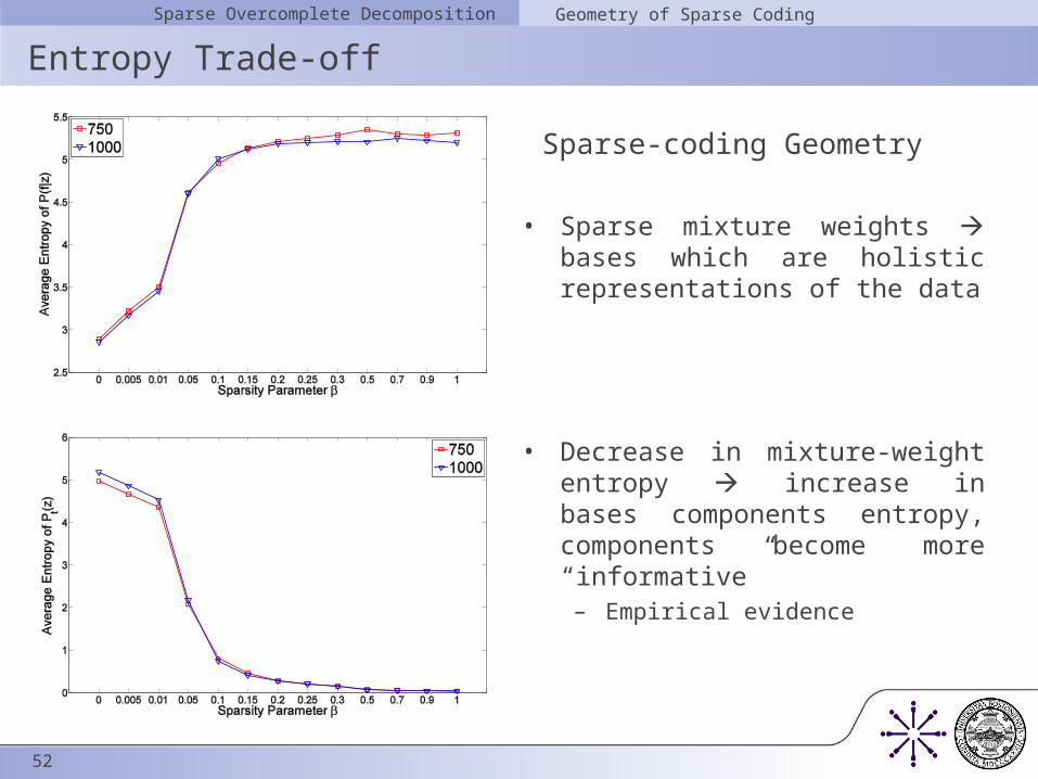
Entropy Trade-offSparse Overcomplete Decomposition Geometry of Sparse Coding
Sparse-coding Geometry
• Sparse mixture weights bases which are holistic representations of the data
• Decrease in mixture-weight entropy increase in bases components entropy, components become more “informative”
– Empirical evidence
53
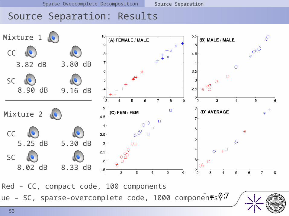
Source Separation: ResultsSparse Overcomplete Decomposition Source Separation
Red – CC, compact code, 100 components
Blue – SC, sparse-overcomplete code, 1000 components, ¯ = 0:7
Mixture 1
Mixture 2
CC
SC
CC
SC
3.82 dB 3.80 dB
9.16 dB8.90 dB
5.25 dB 5.30 dB
8.33 dB8.02 dB

54
Source Separation: ResultsSparse Overcomplete Decomposition Source Separation
Results
• Sparse-overcomplete code leads to better separation
• Separation quality increases with increasing sparsity before tapering off at high sparsity values (> 0.7)
55
Other ApplicationsSparse Overcomplete Decomposition Other Applications
• Framework is general, operates on non-negative data – Text data (word counts), images etc.
• Examples
56
Other ApplicationsSparse Overcomplete Decomposition Other Applications
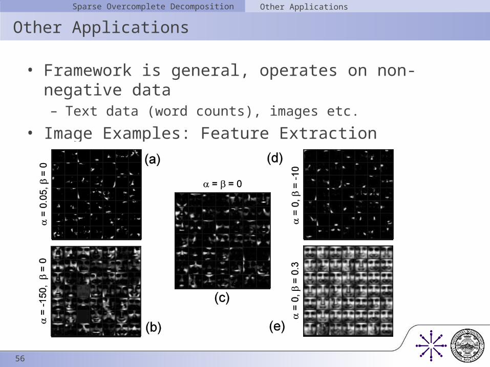
• Framework is general, operates on non-negative data – Text data (word counts), images etc.
• Image Examples: Feature Extraction
57
Other ApplicationsSparse Overcomplete Decomposition Other Applications
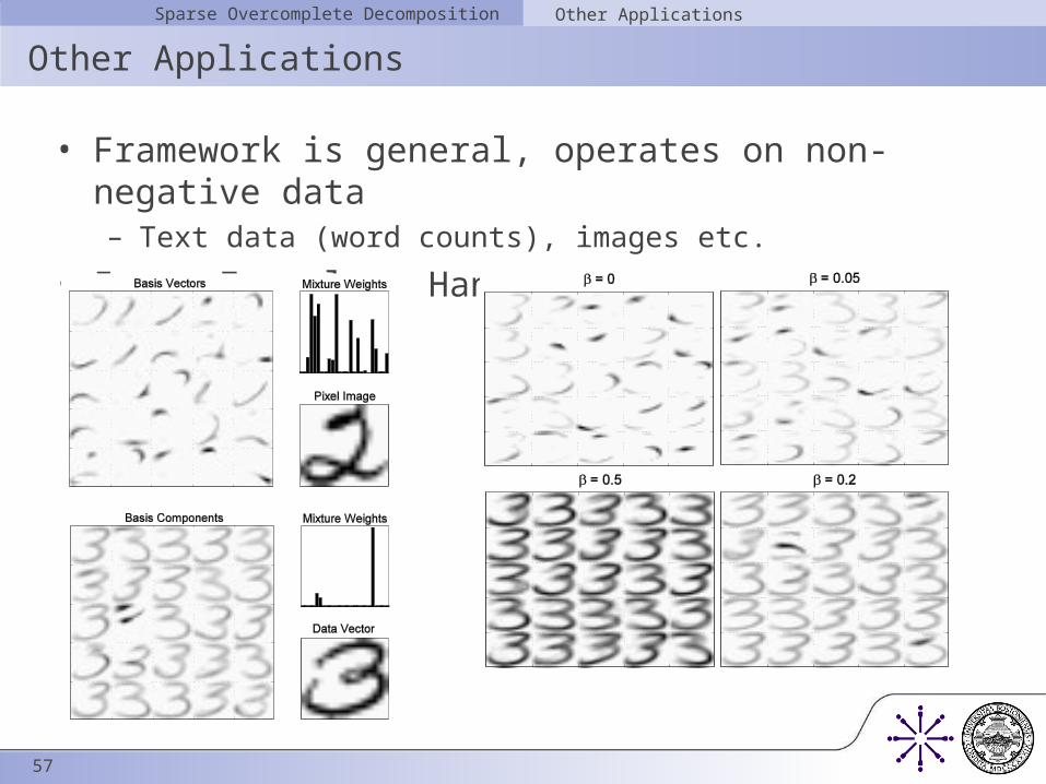
• Framework is general, operates on non-negative data – Text data (word counts), images etc.
• Image Examples: Hand-written digit classification
58
Other ApplicationsSparse Overcomplete Decomposition Other Applications
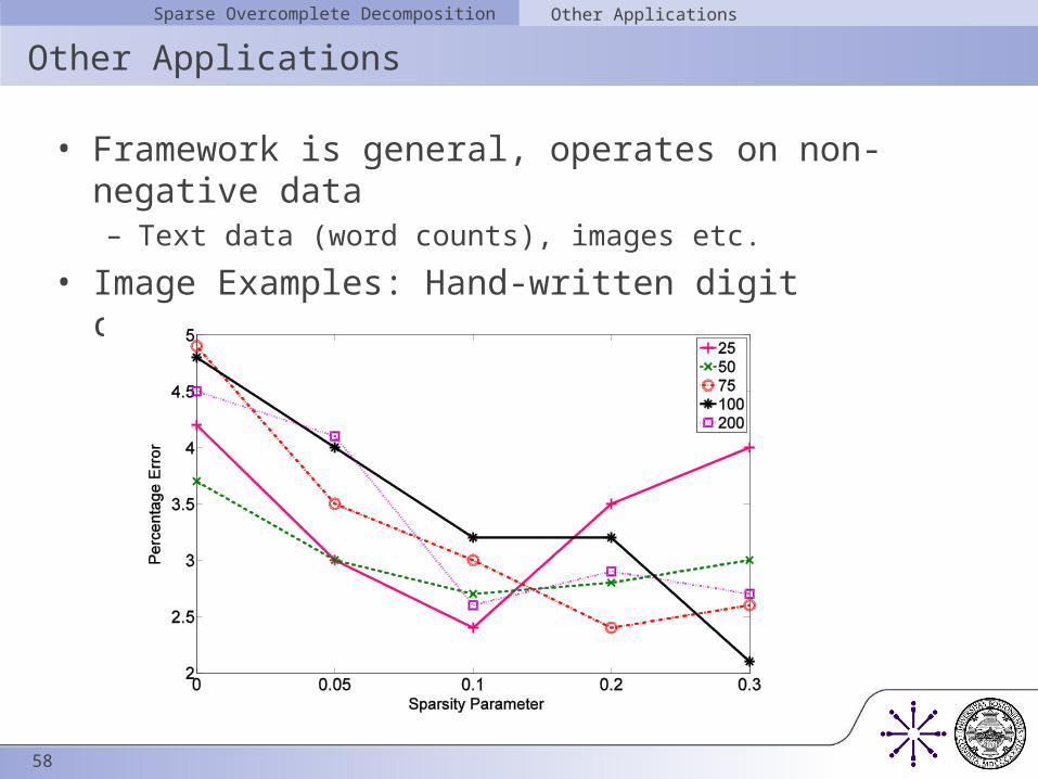
• Framework is general, operates on non-negative data – Text data (word counts), images etc.
• Image Examples: Hand-written digit classification

59
Outline
• Introduction• Time-Frequency Structure• Latent Variable Decomposition: Probabilistic Framework• Sparse Overcomplete Decomposition• Conclusions
– In conclusion…

60
Thesis Contributions
• Modeling single-channel acoustic signals – important applications in various fields
• Provides a probabilistic framework – amenable to principled extensions and improvements
• Incorporates the idea of sparse coding in the framework• Points to other extensions – in the form of priors• Theoretical analysis of models and algorithms• Applicability to other data domains
• Six refereed publications in international conferences and workshops (ICASSP, ICA, NIPS), two manuscripts under review (IEEE TPAMI, NIPS)
Conclusions Thesis Contributions

61
Future Work
• Representation– Other TF representations (eg. constant-Q, gammatone)– Multidimensional representations (correlograms, higher order
spectra)– Utilize phase information in the representation
• Model and Theory
• Applications
Conclusions Future Work
62
Future Work
• Representation
• Model and Theory– Employ priors on parameters to impose known/hypothesized
structure (Dirichlet, mixture Dirichlet, Logistic Normal)– Explicitly model time structure using HMMs/other dynamic models– Utilize discriminative learning paradigm– Extract components that form independent subspaces, could be
used for unsupervised separation– Relation between sparse decomposition and non-negative ICA– Extensions/improvements to inference algorithms (eg. tempered
EM)
• Applications
Conclusions Future Work

63
Future Work
• Representation
• Model and Theory
• Applications – Other audio applications such as music transcription, speaker
recognition, audio classification, language identification etc.– Explore applications in data-mining, text semantic analysis, brain-
imaging analysis, radiology, chemical spectral analysis etc.
Conclusions Future Work
64
Acknowledgements
• Prof. Barbara Shinn-Cunningham• Dr. Bhiksha Raj and Dr. Paris Smaragdis• Thesis Committee Members• Faculty/Staff at CNS and Hearing Research Center• Scientists/Staff at Mitsubishi Electric Research Laboratories• Friends and well-wishers
– Supported in part by the Air Force Office of Scientific Research (AFOSR FA9550-04-1-0260), the National Institutes of Health (NIH R01 DC05778), the National Science Foundation (NSF SBE-0354378), and the Office of Naval Research (ONR N00014-01-1-0624).
– Arts and Sciences Dean’s Fellowship, Teaching Fellowship– Internships at Mitsubishi Electric Research Laboratories
65
Additional Slides

66
Publications
Refereed Publications and Manuscripts Under Review
• MVS Shashanka, B Raj, P Smaragdis. “Probabilistic Latent Variable Model for Sparse Decompositions of Non-negative Data” submitted to IEEE Transactions on Pattern Analysis And Machine Intelligence
• MVS Shashanka, B Raj, P Sparagdis. “Sparse Overcomplete Latent Variable Decomposition of Counts Data” submitted to NIPS 2007
• P Smaragdis, B Raj, MVS Shashanka. “Supervised and Semi-Supervised Separation of Sounds from Single-Channel Mixtures,” Intl. Conf. on ICA, London, Sep 2007
• MVS Shashanka, B Raj, P Smaragdis. “Sparse Overcomplete Decomposition for Single Channel Speaker Separation,” Intl. Conf. on Acoustics, Speech and Signal Processing, Honolulu, Apr 2007
• B Raj, R Singh, MVS Shashanka, P Smaragdis. “Bandwidth Expansion with a Polya Urn Model,” Intl. Conf. on Acoustics, Speech and Signal Proc., Honolulu, Apr 2007
• B Raj, P Smaragdis, MVS Shashanka, R Singh, “Separating a Foreground Singer from Background Music,” Intl Symposium on Frontiers of Research on Speech and Music, Mysore, India, Jan 2007
• P Smaragdis, B Raj, MVS Shashanka. “A Probabilistic Latent Variable Model for Acoustic Modeling ,” Workshop on Advances in Models for Acoustic Processing, NIPS 2006
• B Raj, MVS Shashanka, P Smaragdis. “Latent Dirichlet Decomposition for Single Channel Speaker Separation,” Intl. Conf. on Acoustics, Speech and Signal Processing, Paris, May 2006
Conclusions Thesis Contributions