CO2 Capture by Absorption with Potassium Carbonate

Third Quarterly Report 2005

Quarterly Progress Report

Reporting Period Start Date: July 1, 2005 Reporting Period End Date: September 30, 2005

Authors: Gary T. Rochelle, Marcus Hilliard, Eric Chen, Babatunde Oyenekan, Ross Dugas, John McLees, Andrew Sexton, Daniel Ellenberger

October 26, 2005 DOE Award #: DE-FC26-02NT41440 Department of Chemical Engineering

The University of Texas at Austin

2

Disclaimer This report was prepared as an account of work sponsored by an agency of the United States Government. Neither the United States Government nor any agency thereof, nor any of their employees, makes any warranty, express or implied, or assumes any legal liability or responsibility for the accuracy, completeness, or usefulness of any information, apparatus, product, or process disclosed, or represents that its use would not infringe privately owned rights. Reference herein to any specific commercial product, process, or service by trade name, trademark, manufacturer, or otherwise does not necessarily constitute or imply its endorsement, recommendation, or favoring by the United States Government or any agency thereof. The views and opinions of authors expressed herein do not necessarily state or reflect those of the United States Government or any agency thereof.

3

Abstract The objective of this work is to improve the process for CO2 capture by alkanolamine absorption/stripping by developing an alternative solvent, aqueous K2CO3 promoted by piperazine. Modeling of stripper performance suggests that vacuum stripping may be an attractive configuration for all solvents. Flexipac 1Y structured packing performs in the absorber as expected. It provides twice as much mass transfer area as IMTP#40 dumped packing. Independent measurements of CO2 solubility give a CO2 loading that is 20% lower than that Cullinane’s values with 3.6 m PZ at 100-120oC. The effective mass transfer coefficient (KG) in the absorber with 5 m K/2.5 m PZ appears to be 0 to 30% greater than that of 30 wt% MEA.

4

Contents

Disclaimer ....................................................................................................................................... 2 Abstract ........................................................................................................................................... 3 List of Figures ................................................................................................................................. 6 List of Tables .................................................................................................................................. 8 Introduction..................................................................................................................................... 9 Experimental ................................................................................................................................... 9 Results and Discussion ................................................................................................................... 9 Conclusions................................................................................................................................... 10 Future Work .................................................................................................................................. 11 Task 1 – Modeling Performance of Absorption/Stripping of CO2 with Aqueous K2CO3 Promoted by Piperazine................................................................................................................................. 13

Subtask 1.1 – Modify Vapor-Liquid Equilibrium (VLE) Model...................................... 13 Summary ............................................................................................................... 13 Experimental Section ............................................................................................ 13 Experimental Methods .......................................................................................... 14 Results................................................................................................................... 17 Conclusions........................................................................................................... 20 Future Work .......................................................................................................... 20

Subtask 1.8a – Predict Flowsheet Options – Spreadsheet modeling ................................ 21 Introduction........................................................................................................... 21 Conclusions and Future Work .............................................................................. 32

Subtask 1.8b – Predict Flowsheet Options – Aspen Custom Modeler for Stripper.......... 33 Introduction........................................................................................................... 33 Experimental (Model Formulation) ...................................................................... 33 Results and Discussion ......................................................................................... 37 Conclusions and Future Work .............................................................................. 42

Subtask 1.10 – Simulate MEA Baseline ........................................................................... 43 Summary ............................................................................................................... 43 Results and Discussion ......................................................................................... 43 Conclusions........................................................................................................... 45 Future Work .......................................................................................................... 46

Task 2 – Pilot Plant Testing .......................................................................................................... 47 Subtask 2.6 – Structured Parking – Campaign 4 .............................................................. 47

Introduction........................................................................................................... 47 Experimental – Final Campaign Equipment Modifications ................................. 47 Experimental – Final Campaign Test Plan ........................................................... 48

Task 3 – Solvent Losses................................................................................................................ 51 Subtask 3.1 – Analysis of Degradation Products.............................................................. 51

Introduction........................................................................................................... 51 Experimental ......................................................................................................... 51 Results................................................................................................................... 52 Conclusions and Future Work .............................................................................. 66

Subtask 3.4 – Amine Volatility......................................................................................... 67 Introduction........................................................................................................... 67

5

Experimental Method............................................................................................ 67 Results and Discussion ......................................................................................... 70 Future Work .......................................................................................................... 72

Task 4 – Solvent Reclaiming ........................................................................................................ 73 Subtask 4.2 – Liquid/Liquid Equilibrium ......................................................................... 73

Introduction........................................................................................................... 73 Apparatus .............................................................................................................. 73 Procedure .............................................................................................................. 73 Results................................................................................................................... 74 Conclusions........................................................................................................... 75

References..................................................................................................................................... 75

6

List of Figures

Figure 1 Process Flow Diagram for Solubility of CO2 Experiments, Vapor Phase

Figure 2 Process Flow Diagram for Solubility of CO2 Experiments, Liquid Phase

Figure 3 Process Flow Diagram for the Heat of CO2 Absorption Experiments

Figure 4 CO2 solubility in K+/PZ solutions at 100 °C

Figure 5 CO2 solubility in K+/PZ solutions at 120 °C

Figure 6 Comparison of experimental heat of CO2 absorption measures to Hilliard [2005] predictions for the 5 m K+/2.5 m PZ system from 40-80 °C

Figure 7 Comparison of experimental heat of CO2 absorption measurements to Hilliard [2005] predictions for the 6 m K+/2.5 m PZ system from 40-80 °C

Figure 8 Split Product with Vacuum

Figure 9 Flash Stripping with Split Product and Vacuum Operation

Figure 10 Internal Exchange

Figure 11 Multipressure Stripper

Figure 12 Matrix Stripper

Figure 13 Optimized Lean Concentration for Minimum Equivalent

Figure 14 Total Equivalent Work for Different Configurations with 7m MEA (∆T=10°C)

Figure 15 Total Equivalent Work for Different Configurations with 5m K+/2.5m PZ (∆T=10°C)

Figure 16 Total Equivalent Work for Different ∆T for 5m K+/2.5m PZ

Figure 17 McCabe-Thiele Plot for 5m K+/2.5m PZ, Multipressure Stripper

Figure 18 Pilot Plant Absorber Mass Transfer Data Compared to Wetted Wall Column at 60°C

Figure 19 MEA and Potassium Carbonate/Piperazine Flexipac 1Y Mass Transfer Data Compared to Wetted Wall Column Bench-scale Data at 60°C

Figure 20 Campaign 4 Configuration with Cross-exchanger

Figure 21 1H NMR Analysis of 7 m MEA (200 mM formate, acetate, glycolate, oxalate)

Figure 22 1H NMR Analysis of Sexton 12/14/04 (7 m MEA, 55 °C, α=0.40, 0.2 mM Cu, 1400 RPM)

Figure 23 13C NMR Analysis of 7 m MEA (200 mM formate, acetate, glycolate, oxalate)

Figure 24 13C NMR Analysis of Sexton 12/14/04 (7 m MEA, 55 °C, α=0.40, 0.2 mM Cu, 1400 RPM)

Figure 25 Anion IC Standard (50 ppm acetate, formate, oxalate and glycolate in water)

Figure 26 Anion IC Standard (50 ppm acetate, formate, oxalate, and glycolate in 7 molal MEA)

7

List of Figures (continued) Figure 27 Anion IC Standard (50 ppm acetate, formate, oxalate, glycolate in 5m Pz/2.5 m

KHCO3)

Figure 28 Oxidative degradation of 7 m MEA, 55°C, 1400 RPM, 0.2 mM Cu, 0.4 moles CO2/mole MEA, 98%O2/2%CO2

Figure 29 Oxidative degradation of 7 m MEA, 55°C, 1400 RPM, 0.2 mM Cu, 0.4 moles CO2/mole MEA, 98%O2/2%CO2

Figure 30 Sample Analysis for Experiment 5/3/2005 (55°C, 7 m MEA, α=0.15, Air Agitated Reactor Data, 1400 RPM)

Figure 31 Anion IC Analysis of Sexton Experiment 12/14/05 (7 m MEA, 55 °C, 1400 RPM, 0.2 mM Cu, α=0.40, t=12 days)

Figure 32 FTIR Sampling System for Campaign 4 at PRC

Figure 33 Absorber Gas Outlet Sample Point for Campaign 4 at PRC

Figure 34 Proposed Laboratory Scale Packed Column

8

List of Tables

Table 1 Summary of High Temperature VLE Measurements

Table 2 Summary of CO2 Heat of Absorption Measurements

Table 3 Limiting Energy Performance of Innovative Stripper Options with Infinite Contacting Capability

Table 4 Adjustable Constants in VLE Expression

Table 5 Predicted CO2 Solubility at Absorber Conditions

Table 6 Optimal Pressure for different criteria (Rich [CO2]T=3.68m, Tapp=5°C); Constant Treb = 379 K

Table 7 Required Absorber Packing to Emulate Pilot Plant Performance in Aspen

Table 8 Potassium Carbonate/Piperazine Solubility Experiments

Table 9 Product Formation Rates with Inhibitor A in 8 to 16 hours

Table 10 Solubility of Solids with K+/Pz equal to 4

9

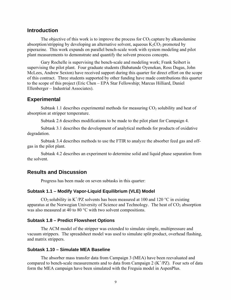
Introduction The objective of this work is to improve the process for CO2 capture by alkanolamine absorption/stripping by developing an alternative solvent, aqueous K2CO3 promoted by piperazine. This work expands on parallel bench-scale work with system modeling and pilot plant measurements to demonstrate and quantify the solvent process concepts.

Gary Rochelle is supervising the bench-scale and modeling work; Frank Seibert is supervising the pilot plant. Four graduate students (Babatunde Oyenekan, Ross Dugas, John McLees, Andrew Sexton) have received support during this quarter for direct effort on the scope of this contract. Three students supported by other funding have made contributions this quarter to the scope of this project (Eric Chen – EPA Star Fellowship; Marcus Hilliard, Daniel Ellenberger – Industrial Associates). Experimental Subtask 1.1 describes experimental methods for measuring CO2 solubility and heat of absorption at stripper temperature.

Subtask 2.6 describes modifications to be made to the pilot plant for Campaign 4.

Subtask 3.1 describes the development of analytical methods for products of oxidative degradation.

Subtask 3.4 describes methods to use the FTIR to analyze the absorber feed gas and off-gas in the pilot plant.

Subtask 4.2 describes an experiment to determine solid and liquid phase separation from the solvent.

Results and Discussion Progress has been made on seven subtasks in this quarter: Subtask 1.1 – Modify Vapor-Liquid Equilibrium (VLE) Model

CO2 solubility in K+/PZ solvents has been measured at 100 and 120 °C in existing apparatus at the Norwegian University of Science and Technology. The heat of CO2 absorption was also measured at 40 to 80 °C with two solvent compositions. Subtask 1.8 – Predict Flowsheet Options

The ACM model of the stripper was extended to simulate simple, multipressure and vacuum strippers. The spreadsheet model was used to simulate split product, overhead flashing, and matrix strippers. Subtask 1.10 – Simulate MEA Baseline

The absorber mass transfer data from Campaign 3 (MEA) have been reevaluated and compared to bench-scale measurements and to data from Campaign 2 (K+/PZ). Four sets of data form the MEA campaign have been simulated with the Freguia model in AspenPlus.

10

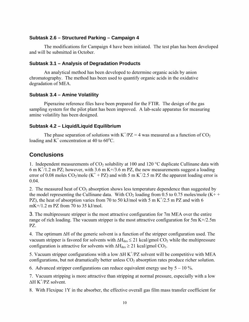
Subtask 2.6 – Structured Parking – Campaign 4

The modifications for Campaign 4 have been initiated. The test plan has been developed and will be submitted in October. Subtask 3.1 – Analysis of Degradation Products

An analytical method has been developed to determine organic acids by anion chromatography. The method has been used to quantify organic acids in the oxidative degradation of MEA.

Subtask 3.4 – Amine Volatility

Piperazine reference files have been prepared for the FTIR. The design of the gas sampling system for the pilot plant has been improved. A lab-scale apparatus for measuring amine volatility has been designed. Subtask 4.2 – Liquid/Liquid Equilibrium

The phase separation of solutions with K+/PZ = 4 was measured as a function of CO2 loading and K+ concentration at 40 to 60oC.

Conclusions 1. Independent measurements of CO2 solubility at 100 and 120 °C duplicate Cullinane data with 6 m K+/1.2 m PZ; however, with 3.6 m K+/3.6 m PZ, the new measurements suggest a loading error of 0.08 moles CO2/mole (K+ + PZ) and with 5 m K+/2.5 m PZ the apparent loading error is 0.04.

2. The measured heat of CO2 absorption shows less temperature dependence than suggested by the model representing the Cullinane data. With CO2 loading from 0.5 to 0.75 moles/mole (K+ + PZ), the heat of absorption varies from 70 to 50 kJ/mol with 5 m K+/2.5 m PZ and with 6 mK+/1.2 m PZ from 70 to 35 kJ/mol.

3. The multipressure stripper is the most attractive configuration for 7m MEA over the entire range of rich loading. The vacuum stripper is the most attractive configuration for 5m K+/2.5m PZ.

4. The optimum ∆H of the generic solvent is a function of the stripper configuration used. The vacuum stripper is favored for solvents with ∆Hdes ≤ 21 kcal/gmol CO2 while the multipressure configuration is attractive for solvents with ∆Hdes ≥ 21 kcal/gmol CO2.

5. Vacuum stripper configurations with a low ∆H K+/PZ solvent will be competitive with MEA configurations, but not dramatically better unless CO2 absorption rates produce richer solution.

6. Advanced stripper configurations can reduce equivalent energy use by 5 – 10 %.

7. Vacuum stripping is more attractive than stripping at normal pressure, especially with a low ∆H K+/PZ solvent.

8. With Flexipac 1Y in the absorber, the effective overall gas film mass transfer coefficient for

11

K+/PZ appears to be 0 to 33% greater than that for MEA. The approximate values of KG vary from 0.0012 to 0.002 mol/m2-s-kPA.

9. As expected the performance of Flexipac 1Y structured packing is better than IMTP#40 random packing, in proportion to the expected wetted surface area.

10. Modeling by AspenPlus suggests confirms the performance of absorber with the IMTP#40. With only two case modeled using Flexipac 1Y, it appears that there is a significant equilibrium pinch in the absorber, which would preclude the calculation of mass transfer performance.

11. Formate, acetate, and oxalate have been identified as significant products in the oxidative degradation of monoethanolamine by anion chromatography and NMR. Two unknown additional unknown peaks are hypothesized to be nitrite and nitrate.

12. It should be possible to use 6.4 m K+/1.6 m PZ in the pilot plant without precipitating additional solid phases at 40oC.

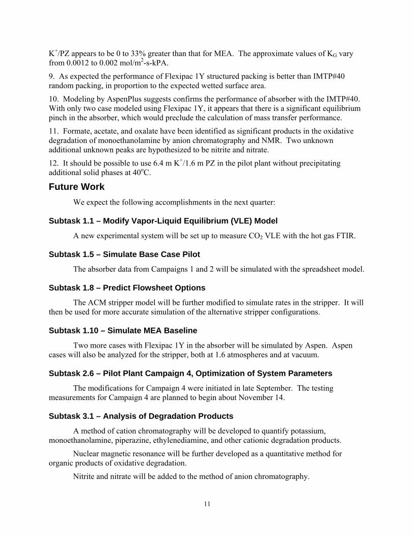
Future Work We expect the following accomplishments in the next quarter: Subtask 1.1 – Modify Vapor-Liquid Equilibrium (VLE) Model

A new experimental system will be set up to measure CO2 VLE with the hot gas FTIR. Subtask 1.5 – Simulate Base Case Pilot

The absorber data from Campaigns 1 and 2 will be simulated with the spreadsheet model. Subtask 1.8 – Predict Flowsheet Options

The ACM stripper model will be further modified to simulate rates in the stripper. It will then be used for more accurate simulation of the alternative stripper configurations.

Subtask 1.10 – Simulate MEA Baseline

Two more cases with Flexipac 1Y in the absorber will be simulated by Aspen. Aspen cases will also be analyzed for the stripper, both at 1.6 atmospheres and at vacuum.

Subtask 2.6 – Pilot Plant Campaign 4, Optimization of System Parameters

The modifications for Campaign 4 were initiated in late September. The testing measurements for Campaign 4 are planned to begin about November 14.

Subtask 3.1 – Analysis of Degradation Products

A method of cation chromatography will be developed to quantify potassium, monoethanolamine, piperazine, ethylenediamine, and other cationic degradation products.

Nuclear magnetic resonance will be further developed as a quantitative method for organic products of oxidative degradation.

Nitrite and nitrate will be added to the method of anion chromatography.

12

Subtask 3.4 – Amine Volatility

A bench-scale apparatus will be constructed and tested for measuring amine volatility at absorber conditions.

13

Task 1 – Modeling Performance of Absorption/Stripping of CO2 with Aqueous K2CO3 Promoted by Piperazine Subtask 1.1 – Modify Vapor-Liquid Equilibrium (VLE) Model by Marcus Hilliard

(Supported by the Industrial Associates Program and the Norwegian University of Science and Technology)

with assistance from Inna Kim (Supported by Norwegian University of Science and Technology)

Summary

Cullinane (2005) measured speciation at 40 to 60 oC and CO2 solubility at 40 to 110 oC with a wide range of solution compositions in PZ/K2CO3. When Cullinane (2005) and Hilliard (2005) regressed these data with the electrolyte-NRTL model they found that the apparent heat of CO2 desorption was unexpectedly a significant function of temperature. This work is a collaborative effort of The University of Texas at Austin and the Norwegian University of Science and Technology to generate data by independent methods to confirm the heat of desorption and CO2 solubility at stripper conditions.

Experimental Section

Sample solutions of K2CO3, potassium bicarbonate (KHCO3), and piperazine (PZ) were prepared from Flucka and Sigma-Aldrich, respectively, without further purification and deionized water. CO2 and nitrogen (N2) gases were obtained from AGA Gas GmbH at a purity of >99.99 mol% and >99.999 mol%, respectively.

Solubility and heat of CO2 absorption was measured in a VLE apparatus with vapor recirculation and in a heat balance calorimeter with aqueous K2CO3/PZ/CO2 (Tables 1 and 2).

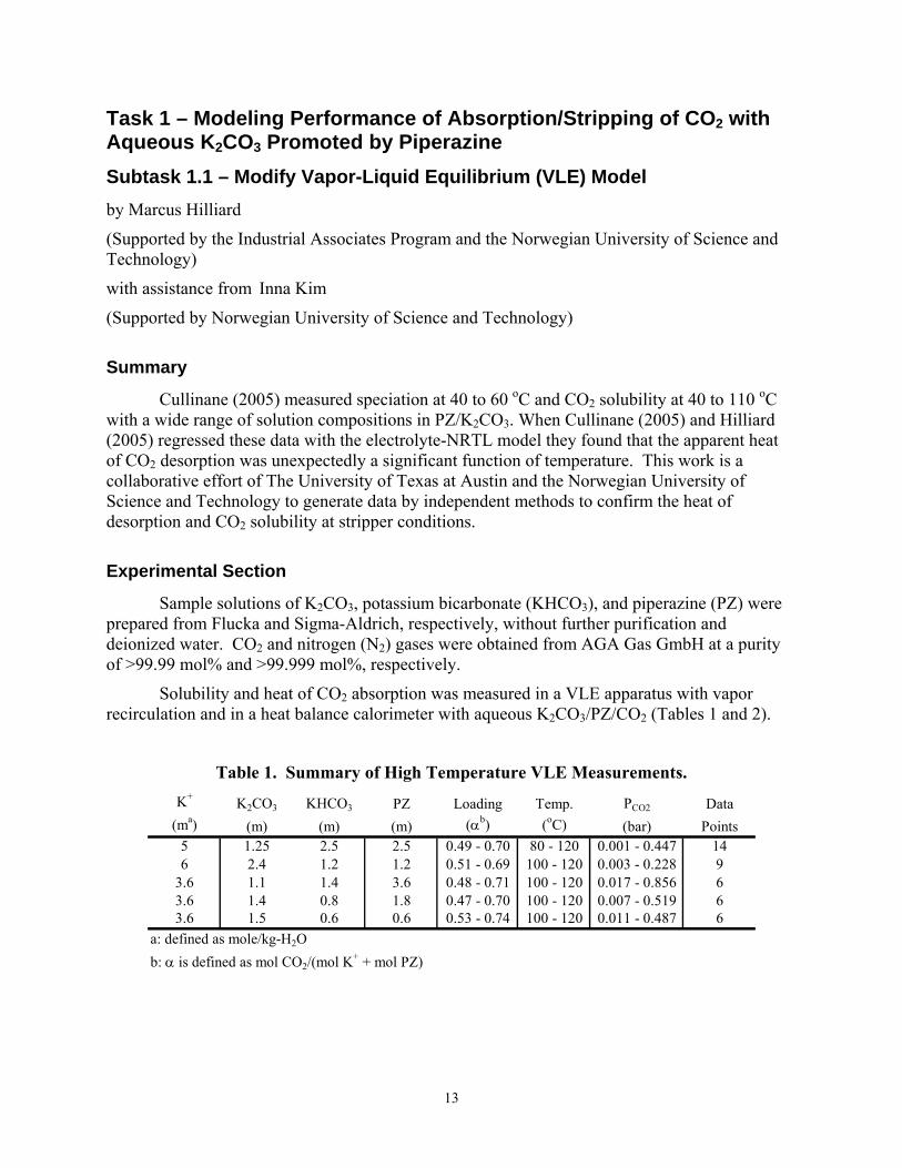
Table 1. Summary of High Temperature VLE Measurements. K+ K2CO3 KHCO3 PZ Loading Temp. PCO2 Data

(ma) (m) (m) (m) (αb) (oC) (bar) Points5 1.25 2.5 2.5 0.49 - 0.70 80 - 120 0.001 - 0.447 146 2.4 1.2 1.2 0.51 - 0.69 100 - 120 0.003 - 0.228 9

3.6 1.1 1.4 3.6 0.48 - 0.71 100 - 120 0.017 - 0.856 63.6 1.4 0.8 1.8 0.47 - 0.70 100 - 120 0.007 - 0.519 63.6 1.5 0.6 0.6 0.53 - 0.74 100 - 120 0.011 - 0.487 6

a: defined as mole/kg-H2Ob: α is defined as mol CO2/(mol K+ + mol PZ)

14

Table 2. Summary of CO2 Heat of Absorption Measurements. K+ K2CO3 KHCO3 PZ Loading Temp. Dhabs Data

(ma) (m) (m) (m) (αb) (oC) (kJ/mol-CO2) Points5 1.25 2.5 2.5 0.49 - 0.70 40 - 80 16.6 - 72.2 526 2.4 1.2 1.2 0.51 - 0.69 40 - 80 20.8 - 64.3 43

a: defined as mole/kg-H2Ob: α is defined as mol CO2/(mol K+ + mol PZ)

Experimental Methods

CO2 Solubility

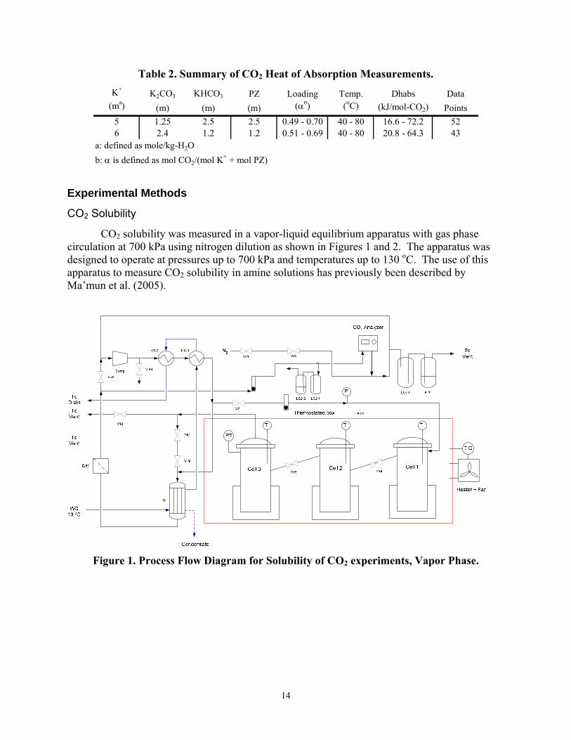
CO2 solubility was measured in a vapor-liquid equilibrium apparatus with gas phase circulation at 700 kPa using nitrogen dilution as shown in Figures 1 and 2. The apparatus was designed to operate at pressures up to 700 kPa and temperatures up to 130 oC. The use of this apparatus to measure CO2 solubility in amine solutions has previously been described by Ma’mun et al. (2005).

Figure 1. Process Flow Diagram for Solubility of CO2 experiments, Vapor Phase.

15

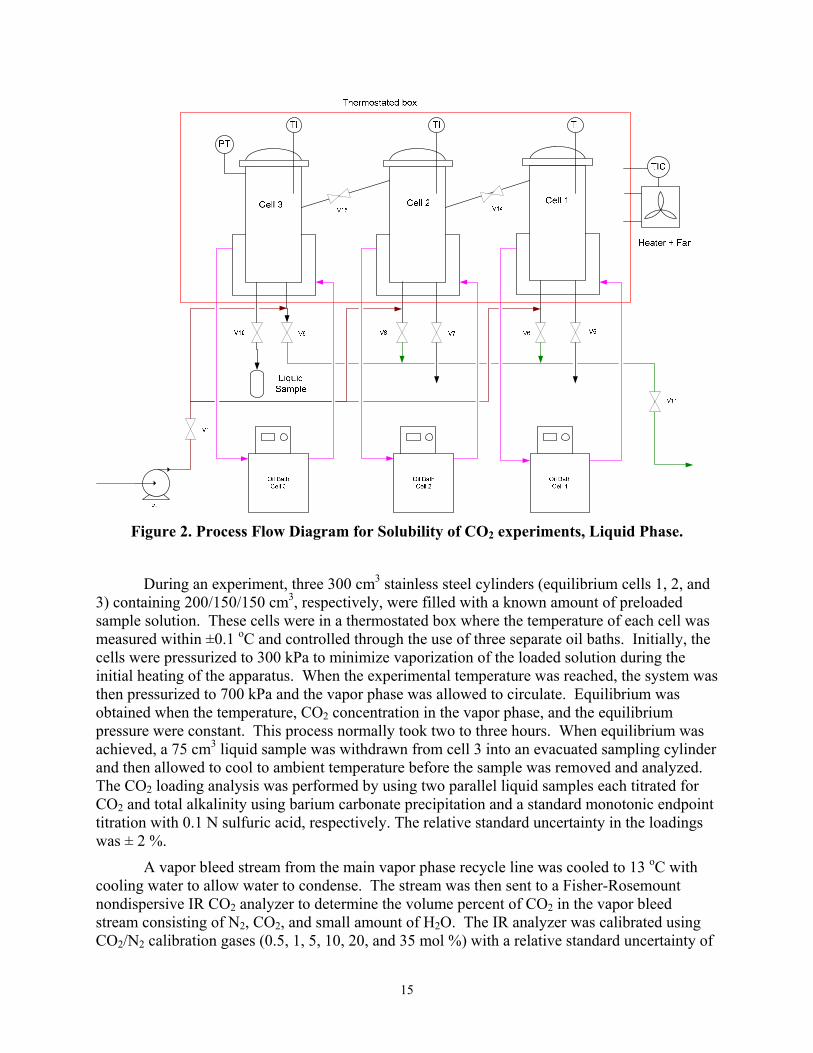
Figure 2. Process Flow Diagram for Solubility of CO2 experiments, Liquid Phase.

During an experiment, three 300 cm3 stainless steel cylinders (equilibrium cells 1, 2, and 3) containing 200/150/150 cm3, respectively, were filled with a known amount of preloaded sample solution. These cells were in a thermostated box where the temperature of each cell was measured within ±0.1 oC and controlled through the use of three separate oil baths. Initially, the cells were pressurized to 300 kPa to minimize vaporization of the loaded solution during the initial heating of the apparatus. When the experimental temperature was reached, the system was then pressurized to 700 kPa and the vapor phase was allowed to circulate. Equilibrium was obtained when the temperature, CO2 concentration in the vapor phase, and the equilibrium pressure were constant. This process normally took two to three hours. When equilibrium was achieved, a 75 cm3 liquid sample was withdrawn from cell 3 into an evacuated sampling cylinder and then allowed to cool to ambient temperature before the sample was removed and analyzed. The CO2 loading analysis was performed by using two parallel liquid samples each titrated for CO2 and total alkalinity using barium carbonate precipitation and a standard monotonic endpoint titration with 0.1 N sulfuric acid, respectively. The relative standard uncertainty in the loadings was ± 2 %.

A vapor bleed stream from the main vapor phase recycle line was cooled to 13 oC with cooling water to allow water to condense. The stream was then sent to a Fisher-Rosemount nondispersive IR CO2 analyzer to determine the volume percent of CO2 in the vapor bleed stream consisting of N2, CO2, and small amount of H2O. The IR analyzer was calibrated using CO2/N2 calibration gases (0.5, 1, 5, 10, 20, and 35 mol %) with a relative standard uncertainty of

16

± 2 %.

The concentration of amine in the vapor bleed stream was assumed to have condensed into the water condensate due to the low vapor pressure of the amine at 13 oC. The partial pressure of water after the condenser was assumed to be the vapor pressure of water at 13 oC. As noncondensable gases, the amount of N2 was assumed to be the same before and after the condenser. Thus, the partial pressure of CO2 can be calculated from the following equation:

( )2 2 22IR IR

CO CO H O H O PZ PZP y P P P P Ldg P= − + − − ⋅ (1)

where

P is the total pressure, kPa, 2

IRCOy is the volume percent of CO2 from the IR analyzer, %,

iP is the partial pressure of component i, kPa, Ldg is the loading of the liquid condensate.

Through liquid analysis, it was found that the water condensate collected from the vapor bleed stream during the experiment contained trace amounts of dissolved CO2 and amine. The CO2 concentration in the condensate was estimated by a correlation of limited data from analyses of the condensate:

( )2

+2mol CO mol K0.6913 0.0498 ln 0.0163

mol PZ mol PZCOLdg P ⎛ ⎞⎛ ⎞ = + ⋅ − ⋅⎜ ⎟ ⎜ ⎟⎝ ⎠ ⎝ ⎠

(2)

Enthalpies of CO2 absorption

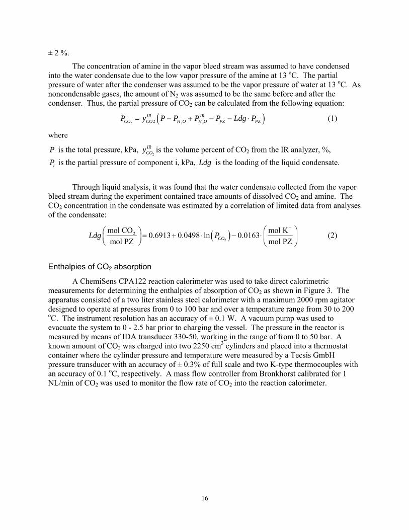
A ChemiSens CPA122 reaction calorimeter was used to take direct calorimetric measurements for determining the enthalpies of absorption of CO2 as shown in Figure 3. The apparatus consisted of a two liter stainless steel calorimeter with a maximum 2000 rpm agitator designed to operate at pressures from 0 to 100 bar and over a temperature range from 30 to 200 oC. The instrument resolution has an accuracy of ± 0.1 W. A vacuum pump was used to evacuate the system to 0 - 2.5 bar prior to charging the vessel. The pressure in the reactor is measured by means of IDA transducer 330-50, working in the range of from 0 to 50 bar. A known amount of CO2 was charged into two 2250 cm3 cylinders and placed into a thermostat container where the cylinder pressure and temperature were measured by a Tecsis GmbH pressure transducer with an accuracy of ± 0.3% of full scale and two K-type thermocouples with an accuracy of 0.1 oC, respectively. A mass flow controller from Bronkhorst calibrated for 1 NL/min of CO2 was used to monitor the flow rate of CO2 into the reaction calorimeter.

17

Figure 3. Process Flow Diagram for the Heat of CO2 Absorption Experiments.

Before starting the experiment, the total CO2 and amine concentration in the experimental solution was determined through barium carbonate precipitation and a standard monotonic endpoint titration with 0.1 N sulfuric acid, respectively. Then, the solution reservoir was flushed with N2 filled with the experimental solution and weighed. The calorimeter was evacuated to a pressure between 0 - 2.5 bar prior to charging the vessel with CO2. This procedure was completed twice to ensure proper evacuation and to prevent contamination of the experimental solution. Approximately 1 - 1.5 kg of the experimental solution was then transferred to the calorimeter where the apparatus was then sealed. The solution reservoir was weighed to determine the exact amount of solution transfer. The system was allowed to come to equilibrium at a desired temperature to obtain a baseline reading of the heat flow. On average, 0.26 moles of CO2 was then fed into the calorimeter and allowed to come to equilibrium before the next amount of CO2 was introduced and continued until the solution was saturated. The number of moles of CO2 in the calorimeter was determined utilizing the Peng-Robinson Equation of State (PR). PR was used to calculate the number of moles of CO2 that were fed into the calorimeter initially and the moles of CO2 in the calorimeter gas phase at equilibrium. The number of moles of CO2 that reacted could then be calculated. The heat flow through the calorimeter during the experiment could be integrated at each point to give the amount of heat that was absorbed by the thermostating liquid or the amount of heat released due to the net heat of absorption with CO2.

Results

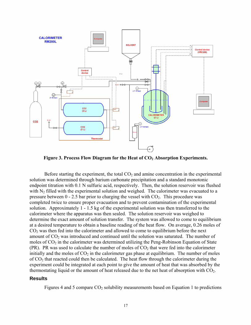
Figures 4 and 5 compare CO2 solubility measurements based on Equation 1 to predictions

18

as reported by Hilliard (2005) for K+/PZ solutions at 100 and 120 oC. Previous model predictions seem to over predict the new experimental data from this study by 30 % at 100 oC and 5 % at 120 oC. The over prediction could be a systematic error in the measured loading of these data or of the original Cullinane data.

100

1000

10000

100000

0.45 0.50 0.55 0.60 0.65 0.70 0.75

Loading (mol CO2/mol K+ + mol PZ)

P CO

2 (Pa

)

3.6 m K+/3.6 m PZ

5 m K+/2.5 m PZ

3.6 m K+/1.8 m PZ

6.0 m K+/1.2 m PZ

3.6 m K+/0.6 m PZ

Figure 4. CO2 solubility in K+/PZ solutions at 100 oC. Solid Points: Measurements

Corrected for H2O Condensate Loading, Lines: Predicted by Hilliard [2005].

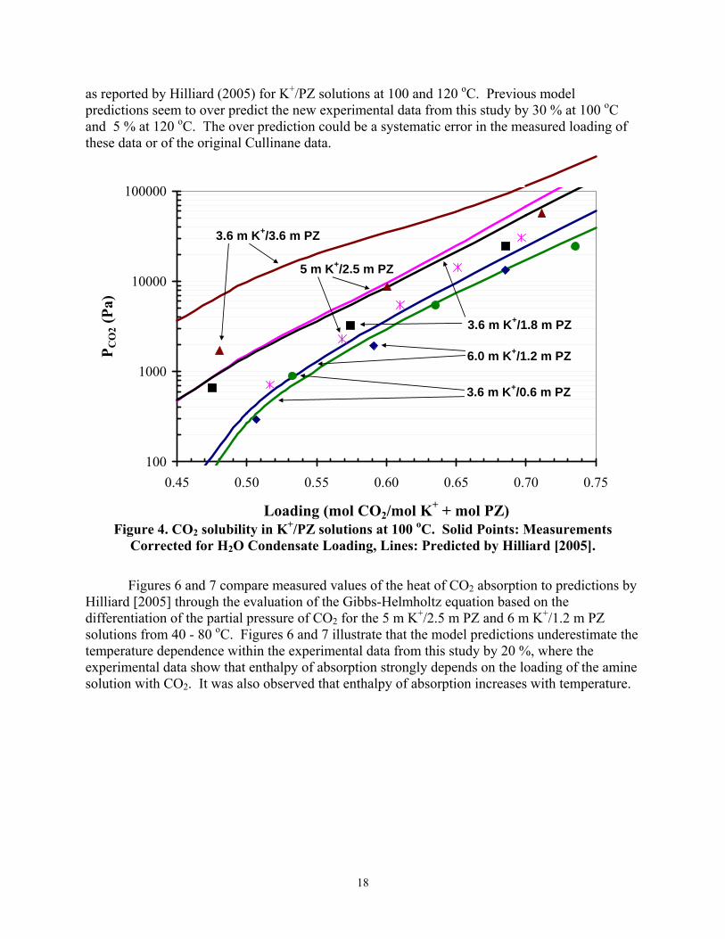
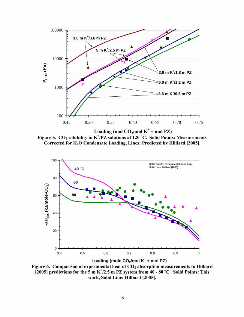
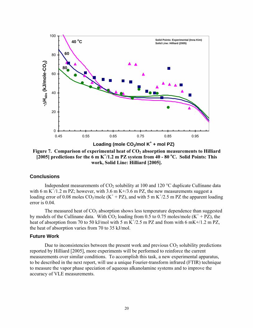
Figures 6 and 7 compare measured values of the heat of CO2 absorption to predictions by Hilliard [2005] through the evaluation of the Gibbs-Helmholtz equation based on the differentiation of the partial pressure of CO2 for the 5 m K+/2.5 m PZ and 6 m K+/1.2 m PZ solutions from 40 - 80 oC. Figures 6 and 7 illustrate that the model predictions underestimate the temperature dependence within the experimental data from this study by 20 %, where the experimental data show that enthalpy of absorption strongly depends on the loading of the amine solution with CO2. It was also observed that enthalpy of absorption increases with temperature.

19

100

1000

10000

100000

0.45 0.50 0.55 0.60 0.65 0.70 0.75

Loading (mol CO2/mol K+ + mol PZ)

P CO

2 (Pa

)3.6 m K+/3.6 m PZ

5 m K+/2.5 m PZ

3.6 m K+/1.8 m PZ

6.0 m K+/1.2 m PZ

3.6 m K+/0.6 m PZ

Figure 5. CO2 solubility in K+/PZ solutions at 120 oC. Solid Points: Measurements

Corrected for H2O Condensate Loading, Lines: Predicted by Hilliard [2005].

0

20

40

60

80

100

0.4 0.5 0.6 0.7 0.8 0.9 1

Loading (mole CO2/mol K+ + mol PZ)

- ∆H

abs (

kJ/m

ole-

CO

2) 60

Solid Points: Experimental (Inna Kim)Solid Line: Hilliard (2005)40 oC

80

Figure 6. Comparison of experimental heat of CO2 absorption measurements to Hilliard

[2005] predictions for the 5 m K+/2.5 m PZ system from 40 - 80 oC. Solid Points: This work, Solid Line: Hilliard [2005].

20

0

20

40

60

80

100

0.45 0.55 0.65 0.75 0.85 0.95

Loading (mole CO2/mol K+ + mol PZ)

- ∆H

abs (

kJ/m

ole-

CO

2)40 oC Solid Points: Experimental (Inna Kim)

Solid Line: Hilliard (2005)

60

80

Figure 7. Comparison of experimental heat of CO2 absorption measurements to Hilliard

[2005] predictions for the 6 m K+/1.2 m PZ system from 40 - 80 oC. Solid Points: This work, Solid Line: Hilliard [2005].

Conclusions

Independent measurements of CO2 solubility at 100 and 120 °C duplicate Cullinane data with 6 m K+/1.2 m PZ; however, with 3.6 m K+/3.6 m PZ, the new measurements suggest a loading error of 0.08 moles CO2/mole (K+ + PZ), and with 5 m K+/2.5 m PZ the apparent loading error is 0.04.

The measured heat of CO2 absorption shows less temperature dependence than suggested by models of the Cullinane data. With CO2 loading from 0.5 to 0.75 moles/mole (K+ + PZ), the heat of absorption from 70 to 50 kJ/mol with 5 m K+/2.5 m PZ and from with 6 mK+/1.2 m PZ, the heat of absorption varies from 70 to 35 kJ/mol.

Future Work

Due to inconsistencies between the present work and previous CO2 solubility predictions reported by Hilliard [2005], more experiments will be performed to reinforce the current measurements over similar conditions. To accomplish this task, a new experimental apparatus, to be described in the next report, will use a unique Fourier-transform infrared (FTIR) technique to measure the vapor phase speciation of aqueous alkanolamine systems and to improve the accuracy of VLE measurements.

21

Subtask 1.8a – Predict Flowsheet Options – Spreadsheet modeling By Gary Rochelle

(Supported by this contract and by the University academic budget)

Introduction

Our modeling of simple and multipressure stripper configurations suggests that the optimum generic solvent is one with a higher heat of desorption than MEA. Since potassium carbonate/piperazine can be customized with a heat of desorption from 10 to 18 kcal/gmol and this is less than 22 kcal/gmol for MEA, it is improbable that it can be used in a simple stripper with a lower energy requirement than MEA.

The PZ/K solvent has three potential significant differences that may be exploited in optimized stripper configurations:

1. A much lower heat of desorption (10 kcal/gmol CO2 with 6.2 m K+/1.2 m PZ).

a. This will be inherently better than MEA for a more isothermal operation and lends itself to stripping at vacuum.

b. With less heat going to reversing the reaction, more heat will be available in the stripper offgas for heat recovery by configurations such as multieffect stripping.

2. Faster rates of absorption, permitting richer solutions than MEA.

a. Richer solutions should be more attractive in optimized configurations that generate CO2 at greater pressure, such as the multipressure configuration.

3. Stripping at higher temperature and pressure.

Because piperazine is not subject to the same chemistry of thermal degradation as MEA, it may be possible to operate the stripper at greater temperature and pressure with 5 m K+/2.5 m PZ. The heat duty and total energy requirement may decrease because of the greater temperature swing, giving an effect similar to a greater heat of desorption.

Depending on the conditions, the PZ/K solvent may have a somewhat lower capacity than 30% MEA.

Therefore there may be specific advanced stripper configurations that will be more attractive with the PZ/K solvent.

Analysis of the baseline configuration

Simple stripping has some inherent short-comings that reduce efficiency and require more heat.

1. Temperature change across the stripper – Because the H2O mole fraction in the gas increases from near 100% in the bottom of the stripper to as little as 20% in the stripper overhead, the temperature decreases by 15 to 25o C from the bottom to the top of an isobaric stripper. Pressure drop in the stripper will increase this even further.

a. The specific reboiler heat duty (kcal/gmol CO2) to provide sensible heat for the solvent

22

depends inversely on the capacity of the solvent:

Qsensiible (kcal/gmol CO2) = Cp∆T/Capacity

e.g. Qsensible = 1 kcal/kg-soln-oC * 15C / 0.5 gmol CO2/kg-soln (3)

30 kcal/gmol CO2

This is severe penalty for lower capacity solvents. It places a premium on capacity and rewards overstripping below the lean loading required for adequate absorber performance in order to enhance capacity, even though overstripping is thermodynamically irreversible and results in excessive driving force at the lean end of the absorber.

b. The temperature change also limits the benefits of richer feed. As less water vapor is required in the stripper overhead because of richer solution with an inherently lower P*

H2O/P*CO2, the

temperature difference across the stripper will increase. Therefore the primary benefit of rich feed is to increase the working capacity of the solvent.

c. The large temperature change across the stripper results in a mismatch of the heating and cooling requirements for the cross-exchanger. Since a large cross exchanger can provide a 5 to 10 °C approach, the rich feed can be heated well above its bubble point. Such a flashing feed can generate operating problems if it is allowed to flash in the feed piping. The flash at the top of the column is irreversible and creates a loss of available work. The released vapor is not as effective at stripping CO2 as steam introduced to the reboiler, so it is not effective use of the available heat in the hot lean solution. Furthermore, flashing of the feed gives more water vapor in the overhead product than expected with a more reversible top feed.

2. Rich end pinch and overstripping

The need to provide sensible heat to the solvent as it passes down the column condenses water vapor. Therefore the L/G is greater at the top of the column. This effect is magnified with solvents that have a heat of desorption greater than 10 kcal/gmol because it takes more than one mole of water vapor in the bottom of the column to end up with one mole of CO2 at the top. As a result stripper performance is frequently determined by a rich end pinch. The operating line is curved. The reboiler duty is simply the sum of the heat of CO2 desorption, the sensible heat of the solvent, and the latent heat of water in the overhead vapor. The amount of water in overhead vapor is determined in the ideal limit by the bubble point temperature of the feed at the pressure of the column. With a rich end pinch the driving force at the lean end of the column can be excessively large, resulting in loss of available work.

Because of the rich end pinch, the optimum design of a simple stripper frequently results in overstripping of the lean product. The lean loading that minimizes heat duty is much lower than needed to achieve adequate absorber performance. Although this optimization gives a reasonably reversible stripper, the absorber has an excessive lean end driving force where available work is lost.

3. Loss of latent heat in CO2 product

Typically the vapor CO2 product includes 0.5 to 2 moles water vapor/mole CO2. This represents a large loss of available work if it is simply condensed with cooling water. Ideally this latent heat should be recovered. Practically the temperature at which the water condenses drops as heat is recovered, making the heat recovered progressively less valuable. The simple stripper makes no attempt to recover this heat.

23

Vacuum

Operation of the stripper at reduced temperature and pressure addresses some of the system weaknesses. Because it reduces the temperature level of required heat, it can utilize lower pressure, lower value steam. Practically steam would be expanded in a turbine to lower pressure to extract work, then used in the reboiler, so less work energy is lost from the power plant per unit of heat required by stripper.

The reduced temperature level of the reboiler will also facilitate heat recovery. The CO2 compressor can be intercooled to a lower level by exchanging hot gas with the stripper bottom. Hot flue gas can be cooled to a lower level by heating the reboiler bottom. There may be other opportunities for heat recovery in a specific situation.

Because the water vapor leaving the stripper is at a lower pressure/temperature, less available work will be lost when it is cooled and condensed.

A vacuum stripper will facilitate a close approach T in the cross-exchanger, because less heat needs to be exchanged. Close approach T requires large countercurrent exchangers, so feasibility of getting a close approach in only one exchanger can be an important limitation. The requirement of a smaller temperature change will enhance the feasibility of a close approach.

Lower stripper temperature will minimize the thermal degradation of the solvent. The maximum solvent concentration of MEA is limited by thermal degradation, so a lower stripper T will facilitate the use of greater MEA concentration with greater capacity and reduced energy consumption.

Lower stripper temperature will minimize corrosion, which can also constrain MEA concentration. It will also permit the use of plastics and polymers as substitute materials.

Lower stripper temperature reduces the temperature swing that facilitates the stripping of solutions with a greater heat of CO2 desorption. Therefore, it will make the use of low ∆H solvents, such as 6 m K/1.2 M PZ, relatively more attractive than high ∆H solvents.

Lower stripper pressure will require a physically larger CO2 compressor with a somewhat greater compression work requirement. However the total effective work requirement of most solvents is reduced by vacuum stripping because of the use of low pressure steam for the heat source.

Lower stripper temperature will probably require a stripper with a greater diameter and packing height. The diameter must increase to accommodate the greater volume flow of the stripping vapor at reduced density. More packing height may be required because kinetics will be reduced at lower temperature and the mechanism of mass transfer with fast reaction will be slower.

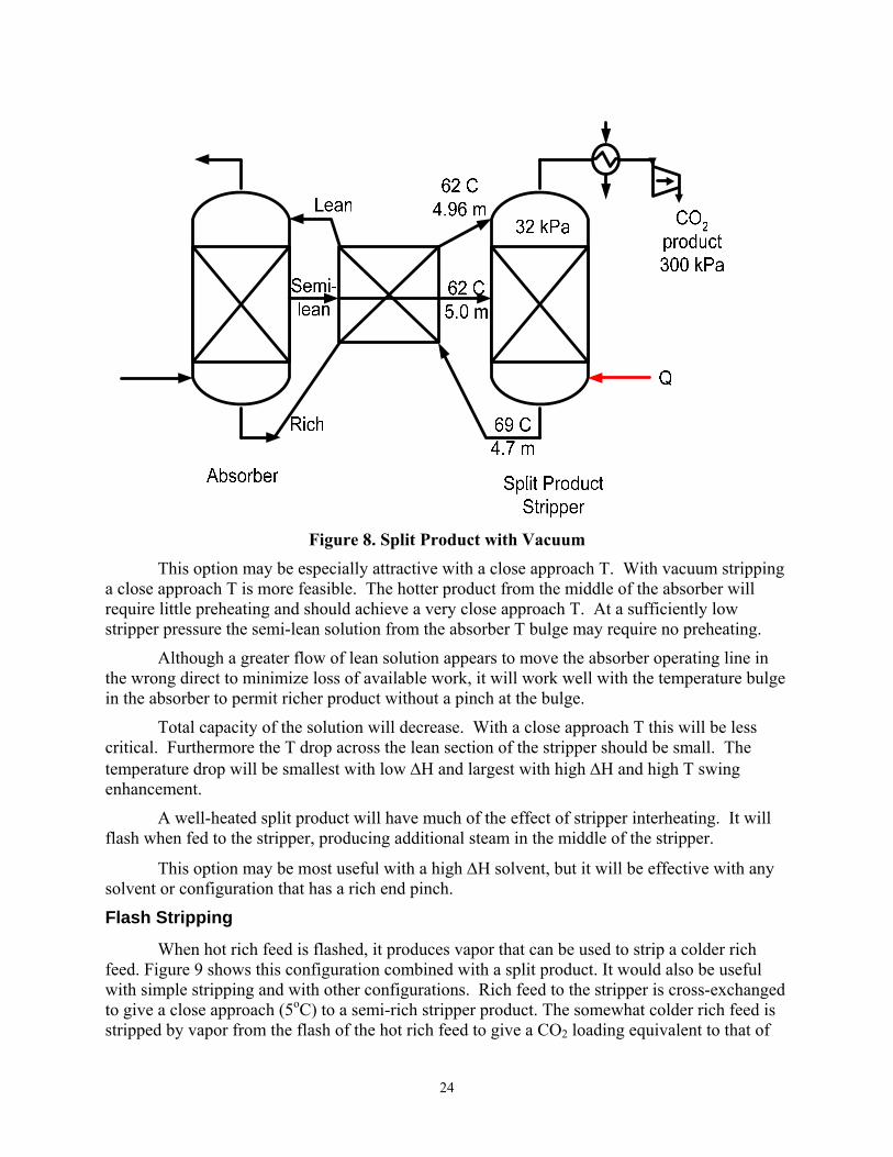
Split Product

Figure 8 illustrates a process utilizing split product to match the operating and equilibrium lines of the stripper. The absorber takes a lean feed and produces rich and semi-rich products. Both products are cross-exchanged to the maximum extent possible and fed to the stripper at the appropriate points. The semi-rich feed will substitute for overstripping providing a lower reboiler T and a smaller ∆T across the stripper, with savings in sensible heat.

24

Figure 8. Split Product with Vacuum

This option may be especially attractive with a close approach T. With vacuum stripping a close approach T is more feasible. The hotter product from the middle of the absorber will require little preheating and should achieve a very close approach T. At a sufficiently low stripper pressure the semi-lean solution from the absorber T bulge may require no preheating.

Although a greater flow of lean solution appears to move the absorber operating line in the wrong direct to minimize loss of available work, it will work well with the temperature bulge in the absorber to permit richer product without a pinch at the bulge.

Total capacity of the solution will decrease. With a close approach T this will be less critical. Furthermore the T drop across the lean section of the stripper should be small. The temperature drop will be smallest with low ∆H and largest with high ∆H and high T swing enhancement.

A well-heated split product will have much of the effect of stripper interheating. It will flash when fed to the stripper, producing additional steam in the middle of the stripper.

This option may be most useful with a high ∆H solvent, but it will be effective with any solvent or configuration that has a rich end pinch.

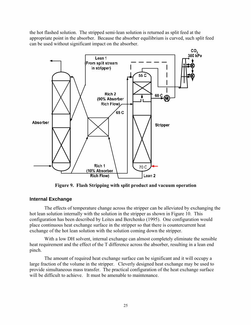
Flash Stripping

When hot rich feed is flashed, it produces vapor that can be used to strip a colder rich feed. Figure 9 shows this configuration combined with a split product. It would also be useful with simple stripping and with other configurations. Rich feed to the stripper is cross-exchanged to give a close approach (5oC) to a semi-rich stripper product. The somewhat colder rich feed is stripped by vapor from the flash of the hot rich feed to give a CO2 loading equivalent to that of

25

the hot flashed solution. The stripped semi-lean solution is returned as split feed at the appropriate point in the absorber. Because the absorber equilibrium is curved, such split feed can be used without significant impact on the absorber.

Figure 9. Flash Stripping with split product and vacuum operation

Internal Exchange

The effects of temperature change across the stripper can be alleviated by exchanging the hot lean solution internally with the solution in the stripper as shown in Figure 10. This configuration has been described by Leites and Berchenko (1995). One configuration would place continuous heat exchange surface in the stripper so that there is countercurrent heat exchange of the hot lean solution with the solution coming down the stripper.

With a low DH solvent, internal exchange can almost completely eliminate the sensible heat requirement and the effect of the T difference across the absorber, resulting in a lean end pinch.

The amount of required heat exchange surface can be significant and it will occupy a large fraction of the volume in the stripper. Cleverly designed heat exchange may be used to provide simultaneous mass transfer. The practical configuration of the heat exchange surface will be difficult to achieve. It must be amenable to maintenance.

26

Figure 10. Internal Exchange

An approximation to internal exchange may be achieved by extracting, exchanging, and returning liquid at one or more points up the stripper.

If internal exchange is effectively implemented with a low ∆H solvent, the energy requirement of a stripper with internal exchange will be limited by a pinch in the bottom lean section. Therefore overstripping will not be attractive. Furthermore it may be attractive to combine internal exchange with split feed from the middle of the stripper to the middle of the absorber.

With a high DH solvent, a stripper with internal exchange may still be limited by a rich end pinch, so overstripping may still be attractive. Therefore, performance may be further enhanced by combining internal exchange with split product to eliminate overstripping.

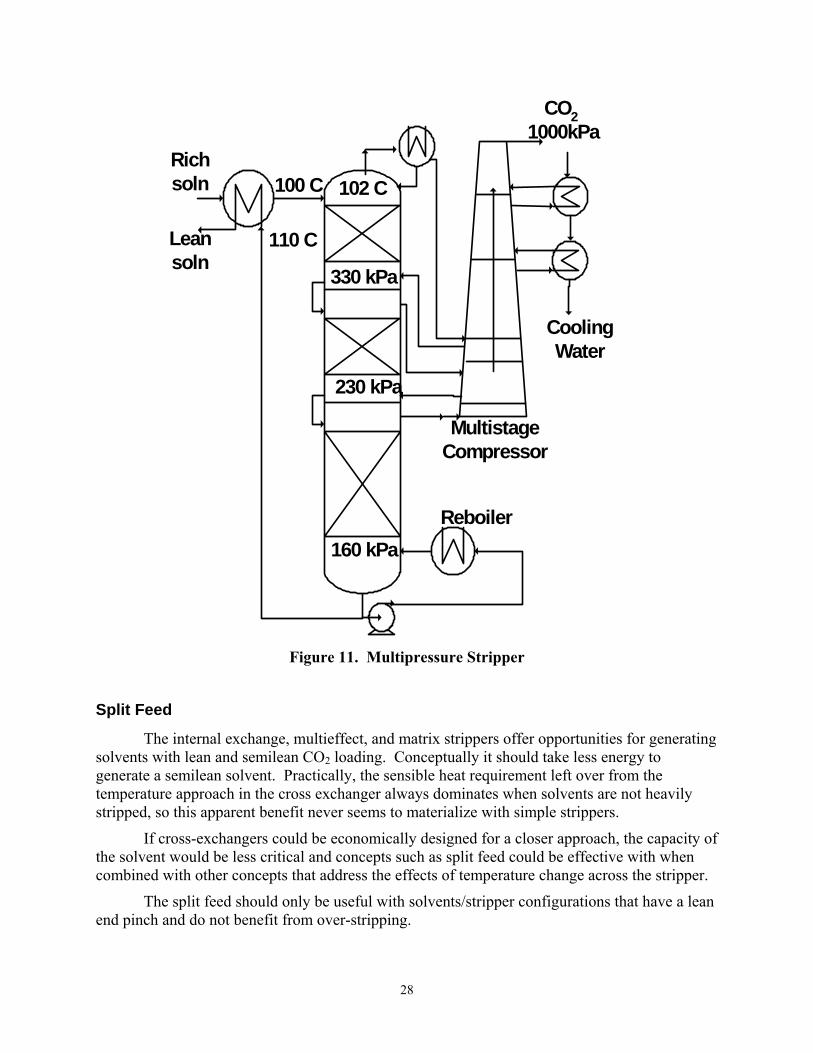
Multipressure Stripper

The multipressure stripper (Figure 11) utilizes mechanical compression of vapor within the stripper to maintain the stripper at near isothermal conditions. As a result, much of the effects of the temperature change across the stripper are eliminated. There is still a tendency toward a rich end pinch, so the optimum lean loading results in overstripping, especially with solvents have a large heat of desorption, such as MEA.

Multipressure stripping can also achieve some effect of heat recovery if the top pressure

27

is operated so that the feed solvent is subcooled, resulting in condensation of most of the water vapor in the overhead CO2 product. This effect is not especially reversible, but the heat is returned into the lower pressure sections with flashing and it is effective in reducing energy requirement in a system with a rich end pinch.

Mechanical compression has an efficiency of about 75%. Since water vapor is being compressed, the overall efficiency of the multipressure option is not high.

Multipressure stripping should be relatively more attractive with richer solutions. Our analyses so far have not demonstrated this effect, perhaps because we have not optimized the overhead pressure. The optimum overhead pressure should increase with richer solutions, but our analyses have usually used only one set of pressures for the multipressure stripper.

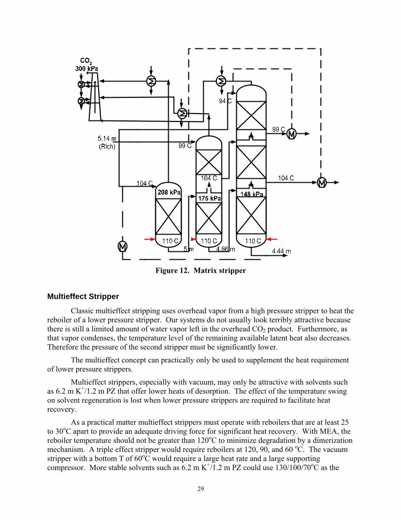
Matrix Stripper

The matrix stripper makes use of two or more strippers at successively lower pressure (Figure 12). Preheated rich solution is fed to the top of each stripper. Semi-rich solution from the first stripper is fed to the bottom section of the second stripper. Semi-rich and semi-lean solution from the second stripper is fed to the third stripper. This pattern can be terminated after three strippers or continued with even more lower pressure strippers. Additional strippers enhance the energy performance at the expense of complexity. The semi-rich, semi-lean, and lean solution from the last stripper is cross-exchanged with rich solution and then returned a split feed to the absorber. The absorber design must use adequate contacting to get good performance with the split feeds.

As a result of the flow configuration, the effects of temperature change across the stripper are alleviated as with the multipressure stripper, but without the inefficiency of mechanical compression.

A solvent with lower heat of desorption, such as 6 m K+/1.5 m PZ, will be relatively more attractive with strippers at lower pressure. Solvents such as MEA rely upon temperature swing regeneration to facilitate stripping. Therefore the matrix configuration should be relatively more attractive with 6.2 m K+/1.2 m PZ.

The opportunities for heat recovery will be enhanced with 6 m K+/1.5 m PZ because more of the stripping heat duty is left over as water vapor in the CO2 product.

The matrix stripper may be ideal for heat recovery by conventional methods such as multieffect stripping and by innovative methods. Because there are multiple strippers, the heat available from a high pressure stripper can be recovered as reboiler duty for a lower pressure stripper.

The matrix configuration requires multiple “strippers”. As a practical matter any full-scale capture system will use multiple strippers. Therefore the matrix configuration would not require additional vessels, but it would increase the complexity of the system.

The matrix configuration requires a CO2 compressor with two initial stages of lower compression ratio with the ability to accept additional gas at each stage.

28

MultistageCompressor

CO2 1000kPa

Reboiler

110 C

100 C

Leansoln

Richsoln 102 C

330 kPa

230 kPa

160 kPa

CoolingWater

Figure 11. Multipressure Stripper

Split Feed

The internal exchange, multieffect, and matrix strippers offer opportunities for generating solvents with lean and semilean CO2 loading. Conceptually it should take less energy to generate a semilean solvent. Practically, the sensible heat requirement left over from the temperature approach in the cross exchanger always dominates when solvents are not heavily stripped, so this apparent benefit never seems to materialize with simple strippers.

If cross-exchangers could be economically designed for a closer approach, the capacity of the solvent would be less critical and concepts such as split feed could be effective with when combined with other concepts that address the effects of temperature change across the stripper.

The split feed should only be useful with solvents/stripper configurations that have a lean end pinch and do not benefit from over-stripping.

29

Figure 12. Matrix stripper

Multieffect Stripper

Classic multieffect stripping uses overhead vapor from a high pressure stripper to heat the reboiler of a lower pressure stripper. Our systems do not usually look terribly attractive because there is still a limited amount of water vapor left in the overhead CO2 product. Furthermore, as that vapor condenses, the temperature level of the remaining available latent heat also decreases. Therefore the pressure of the second stripper must be significantly lower.

The multieffect concept can practically only be used to supplement the heat requirement of lower pressure strippers.

Multieffect strippers, especially with vacuum, may only be attractive with solvents such as 6.2 m K+/1.2 m PZ that offer lower heats of desorption. The effect of the temperature swing on solvent regeneration is lost when lower pressure strippers are required to facilitate heat recovery.

As a practical matter multieffect strippers must operate with reboilers that are at least 25 to 30oC apart to provide an adequate driving force for significant heat recovery. With MEA, the reboiler temperature should not be greater than 120oC to minimize degradation by a dimerization mechanism. A triple effect stripper would require reboilers at 120, 90, and 60 oC. The vacuum stripper with a bottom T of 60oC would require a large heat rate and a large supporting compressor. More stable solvents such as 6.2 m K+/1.2 m PZ could use 130/100/70oC as the

30

reboiler temperatures.

Ultimately the effectiveness of the multieffect stripper will be limited if there is less water vapor in the overhead product. Therefore it will be less attractive with high ∆H solvents that usually have very little water vapor left in the overhead vapor because of the temperature swing desorption.

Feed Preheat

There is an opportunity for the direct or indirect preheat of rich solvent by vapor leaving the stripper. This configuration is not normally attractive because it leaves high temperature heat in the lean stripper bottoms that would otherwise be used to heat the rich solvent. However, because the total heat capacity of the rich solution will be usually be greater than that of the lean solution, it may be attractive to preheat five to twenty percent of the rich solution by exchange with the hot overhead vapor rather than by exchange with the hot lean solution. This will facilitate a close approach temperature at the hot end of the exchange of the lean and rich solution.

Indirect preheat with a heat exchanger cannot do well as preheat with the hot lean solution. Driving force is lost to the boiling point elevation of the solution and to the rapid decrease of water mole fraction as heat is recovered.

Direct countercurrent contact of cold rich solution with the overhead vapor in an additional section of stripper packing can be effective if only a fraction of the rich solution is preheated this way. Even though CO2 will absorb at the cold top of this section, it will desorb in the bottom resulting in a preheated solution with the same loading as the rich feed.

It may be possible to utilize this preheat method with other stripper configurations as a means of recovering latent and sensible heat from the overhead vapor.

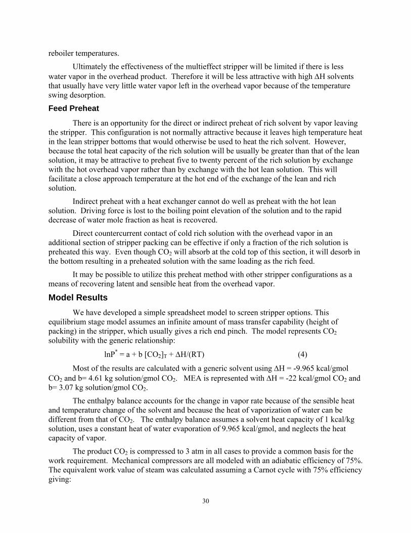
Model Results We have developed a simple spreadsheet model to screen stripper options. This

equilibrium stage model assumes an infinite amount of mass transfer capability (height of packing) in the stripper, which usually gives a rich end pinch. The model represents CO2 solubility with the generic relationship:

lnP* = a + b [CO2]T + ∆H/(RT) (4)

Most of the results are calculated with a generic solvent using ∆H = -9.965 kcal/gmol CO2 and b= 4.61 kg solution/gmol CO2. MEA is represented with ∆H = -22 kcal/gmol CO2 and b= 3.07 kg solution/gmol CO2.

The enthalpy balance accounts for the change in vapor rate because of the sensible heat and temperature change of the solvent and because the heat of vaporization of water can be different from that of CO2. The enthalpy balance assumes a solvent heat capacity of 1 kcal/kg solution, uses a constant heat of water evaporation of 9.965 kcal/gmol, and neglects the heat capacity of vapor.

The product CO2 is compressed to 3 atm in all cases to provide a common basis for the work requirement. Mechanical compressors are all modeled with an adiabatic efficiency of 75%. The equivalent work value of steam was calculated assuming a Carnot cycle with 75% efficiency giving:

31

Weqiv = (Treb (K)+ 10– 313K)/ (Treb(K)+10) (5)

Systems with superheated solvent feed are modeled with an equilibrium flash at the pressure of the stripper. The flash vapor is bypassed to the cumulative overhead vapor.

The results for several cases are presented in Table 3.

Table 3. Limiting energy performance of innovative stripper options with infinite contacting capability.

capacity Comp TotalConfiguration lean rich mol/kg soln app reboil Q Weq W WMEA, ∆H = 22 kcal/gmol, b = 3.07 kg solution/gmol CO2, Simple 0.0059 0.0611 0.61 5 110 30.8 4.69 -0.47 4.21Simple 0.0065 0.0275 0.47 5 110 32.9 5.01 -0.17 4.83Simple 0.0034 0.0275 0.67 10 110 40.0 6.09 -0.17 5.92Simple 0.00003 0.0275 2.18 10 110 34.9 5.32 0.64 5.95simple 0.0060 0.0600 0.76 5 70 36.4 3.09 1.71 4.79flash stripping 0.0060 0.0600 0.66 5 70 34.1 2.89 1.71 4.60split product+flash stripping 0.0060 0.0600 0.30 5 70 45.7 3.87 1.71 5.586 m K/1.2 m PZ, ∆H = 9.965 kcal/gmol, b = 3.30 kg solution/gmol CO2, simple 0.006 0.06 0.7 5 110 38.9 5.31 0.71 6.02simple 0.0056 0.06 0.89 5 70 36.1 3.06 1.98 5.04split product 0.006 0.06 0.7 2 70 31.8 2.70 1.95 4.65split product 0.006 0.06 0.64 5 70 34.8 2.95 1.95 4.90split product+flash stripping 0.006 0.06 0.7 5 70 32.3 2.74 1.95 4.69multipressure 0.006 0.06 0.7 5 70 17.3 1.46 4.37 5.83internal exchange 0.006 0.06 0.7 4 70 31.5 2.66 1.95 4.61internal exchange 0.009 0.08 0.68 4 70 27.8 2.35 1.92 4.27matrix 3 stage 0.006 0.06 0.7 5 70 34.1 2.90 1.82 4.72matrix 4 stage 0.006 0.06 0.7 5 70 32.6 2.70 1.92 4.62

T CEnergy (kcal/gmol CO2)reboilerPCO2* (atm)@40C

The MEA solvent (30 wt %) produces the lowest total work requirement with the simple configuration at normal pressure and none of the innovative configurations are as good as the best conditions with MEA. Most of the calculations were performed with rich solutions giving 0.06 atm CO2. The rich solutions with lower loading (PCO2*=0.0275) require about 12% more equivalent work. The effect of increasing the temperature approach from 5 to 10 °C is to increase total work by about 25%.

The generic solvent with a low heat of absorption (10 kcal/gmol CO2) gives poor performance at normal stripping temperature (110°C), but starts to be competitive with MEA at vacuum stripping temperature (70°C).

Split product appears to be ineffective with MEA systems, which are usually overstripped to maximize solution capacity and minimize energy use. With the low ∆H solvent the split product at vacuum conditions appear to reduce equivalent work by 5%.

Flash stripping produces 4% energy saving for both solvents.

The matrix stripper is 7-9% better than the simple vacuum stripper with the low ∆H

32

solvent. Internal heat exchange also reduces the equivalent work by about 9%.

All of these advanced configurations will probably result in increased capital costs. Therefore, ultimate utility will depend on the tradeoff of capital costs and energy use.

Conclusions and Future Work

Vacuum stripper configurations with a low ∆H K+/PZ solvent will be competitive with MEA configurations, but not dramatically better unless CO2 absorption rates produce richer solution.

Advanced stripper configurations can reduce equivalent energy use by 5 – 10 %.

Vacuum stripping is more attractive than stripping at normal pressure, especially with a low ∆H K+/PZ solvent.

33

Subtask 1.8b – Predict Flowsheet Options – Aspen Custom Modeler for Stripper by Babatunde Oyenekan (Supported by this contract)

Introduction

We have continued to develop the stripper submodel in Aspen Custom Modeler for the overall model of CO2 absorption/stripping for 7m monoethanolamine (MEA), 5m K+ / 2.5m PZ and some generic solvents. This model divides the stripper into sections with Murphree efficiencies assigned to CO2, water and temperature. An expression with six adjustable constants is used to represent the VLE and heat of absorption/desorption for 7m monoethanolamine and 5m K+/2.5m PZ while a three-parameter expression approximates the equilibrium behavior of the generic solvents. Three process configurations (simple, vacuum and multipressure) are simulated and the effect of varying the rich and lean [CO2] T, at a 5-10oC temperature approach on the equivalent work consumed by the process is calculated by this model. The vacuum stripper is favored for solvents with ∆Hdes ≤ 21 kcal/gmol CO2 while the multipressure configuration is attractive for solvents with ∆Hdes ≥ 21 kcal/gmol CO2 at a rich PCO2* = 2.5 kPa and rich absorber temperature of 40oC.

Experimental (Model Formulation)

Stripper Configurations

Simple Stripper

In the conventional configuration, the simple reboiled stripper is run at 160 kPa. The vapor leaving the top of the stripper is cooled and the condensed water is refluxed. The CO2 is compressed in five stages (intercooled to 40oC) to 1000 kPa. The reboiler runs at 110 – 120oC in this configuration.

Multipressure Stripper

In this configuration (Rochelle, 2003), the stripper is divided into three sections, each operating at a different pressure. The CO2 compressor is integrated with the stripper. The vapor from a lower pressure stage is compressed and subsequently used as stripping vapor in a higher-pressure section. Water vapor condenses with the increased pressure and the latent heat of water is recovered. This leads to lower reboiler duties and CO2 is produced at a greater pressure than with the simple (isobaric) stripper. However the compression work is greater than that of the simple stripper because some water vapor is compressed with the CO2. The pressure levels are 160 kPa, 230 kPa and 330 kPa from the bottom to the top of the stripper. The vapor exiting the stripper is cooled and water is refluxed. The CO2 is further compressed in three stages (intercooled to 40oC) to 1000 kPa. Therefore, the five compression stages include two integrated with the stripper.

Multipressure stripping has the following features:

1. The latent heat of water is recovered at the rich end.

34

2. It makes use of the high temperature preheat in the high pressure flash thereby rewarding a closer approach temperature in the cross exchanger.

3. CO2 can be recovered at a greater concentration and pressure. This leads to less compression work downstream of the stripper.

4. This configuration should be best with high ∆Hdes solvents such as 7m MEA.

Vacuum Stripper

This configuration is identical to the simple stripper. The stripper is operated at 30 kPa and the reboiler runs at 60 – 80oC. The CO2 is compressed in five intercooled stages to 1000 kPa.

Vacuum stripping has the following features:

1. Lower temperature (less valuable) steam is used to run the reboiler so more electricity can be extracted before the steam is used in the stripper.

2. Additional compression is required for the CO2.

3. The mass transfer is not as fast as that of the simple stripper because the lower temperature results in slower kinetics.

Aspen Custom Modeler (ACM) Model

A model has been developed in Aspen Custom Modeler to simulate the stripper operation. The model was designed for a wide variety of solvents but has currently been applied to a 7m MEA, 5m K+/2.5m PZ and the generic solvents. Modeling Assumptions

(a) The sections were assumed to be well mixed in the liquid and vapor phases.

(b) The reboiler was assumed to be in equilibrium.

(c) Negligible vaporization of the solvent.

The CO2 vapor pressure (kPa) under stripper conditions for 7m monoethanolamine and 5m K+/2.5m PZ were represented by the linear expression in Table 4. The adjustable constants in Table 4 were obtained by regressing the points for 7m MEA from equilibrium flashes in Aspen Plus using the rigorous model developed by Freguia (2002) from data of Jou and Mather (1995).

35

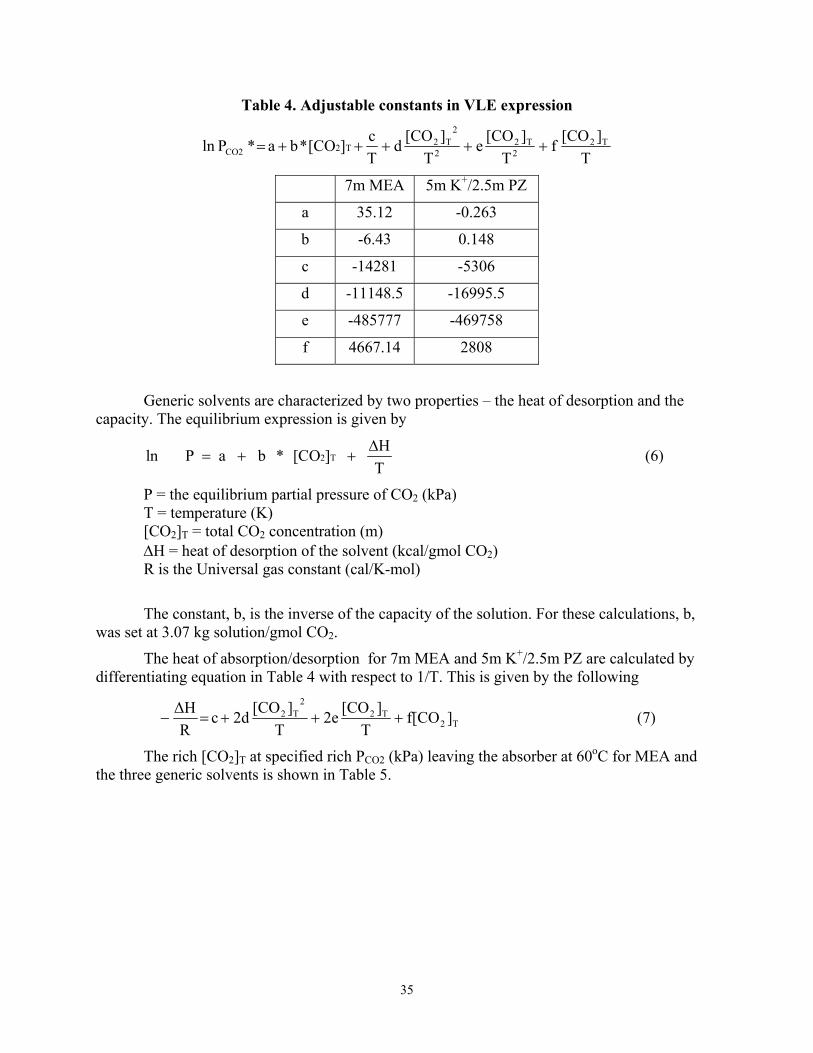
Table 4. Adjustable constants in VLE expression

T][COf

T][COe

T][COd

Tc][CO*ba*Pln T2

2T2

2

2T2T2CO2 +++++=

7m MEA 5m K+/2.5m PZ

a 35.12 -0.263

b -6.43 0.148

c -14281 -5306

d -11148.5 -16995.5

e -485777 -469758

f 4667.14 2808

Generic solvents are characterized by two properties – the heat of desorption and the capacity. The equilibrium expression is given by

2 THln P a b * [CO ]

T∆

= + + (6)

P = the equilibrium partial pressure of CO2 (kPa) T = temperature (K) [CO2]T = total CO2 concentration (m) ∆H = heat of desorption of the solvent (kcal/gmol CO2) R is the Universal gas constant (cal/K-mol)

The constant, b, is the inverse of the capacity of the solution. For these calculations, b, was set at 3.07 kg solution/gmol CO2.

The heat of absorption/desorption for 7m MEA and 5m K+/2.5m PZ are calculated by differentiating equation in Table 4 with respect to 1/T. This is given by the following

T2T2

2T2 ]f[CO

T][CO2e

T][CO2dc

R∆H

+++=− (7)

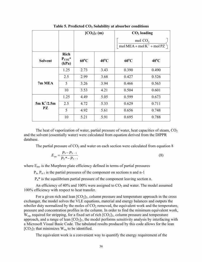
The rich [CO2]T at specified rich PCO2 (kPa) leaving the absorber at 60oC for MEA and the three generic solvents is shown in Table 5.

36

Table 5. Predicted CO2 Solubility at absorber conditions

[CO2]T (m) CO2 loading

⎥⎦

⎤⎢⎣

⎡++ + PZmolKmolMEAmol

COmol 2

Solvent

Rich PCO2* (kPa)

60oC

40oC

60oC

40oC

1.25 2.73 3.43 0.390 0.490

2.5 2.99 3.68 0.427 0.526

5 3.26 3.94 0.466 0.563

7m MEA

10 3.53 4.21 0.504 0.601

1.25 4.49 5.05 0.599 0.673

2.5 4.72 5.33 0.629 0.711

5 4.92 5.61 0.656 0.748

5m K+/2.5m PZ

10 5.21 5.91 0.695 0.788

The heat of vaporization of water, partial pressure of water, heat capacities of steam, CO2 and the solvent (essentially water) were calculated from equation derived from the DIPPR database.

The partial pressure of CO2 and water on each section were calculated from equation 8

1

1

* −

−

−−

=nn

nnmv PP

PPE (8)

where Emv is the Murphree plate efficiency defined in terms of partial pressures

Pn, Pn-1 is the partial pressures of the component on sections n and n-1

Pn* is the equilibrium partial pressure of the component leaving section n.

An efficiency of 40% and 100% were assigned to CO2 and water. The model assumed 100% efficiency with respect to heat transfer.

For a given rich and lean [CO2]T, column pressure and temperature approach in the cross exchanger, the model solves the VLE equations, material and energy balances and outputs the reboiler duty normalized by the moles of CO2 removed, the equivalent work and the temperature, pressure and concentration profiles in the column. In order to find the minimum equivalent work, Weq, required for stripping, for a fixed set of rich [CO2]T, column pressure and temperature approach, and a range of lean [CO2]T, the model performs sensitivity analysis by interfacing with a Microsoft Visual Basic Code. The tabulated results produced by this code allows for the lean [CO2]T that minimizes Weq to be identified.

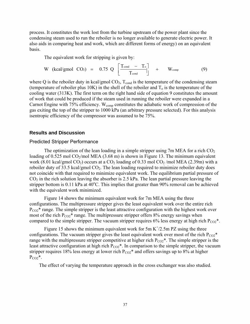
The equivalent work is a convenient way to quantify the energy requirement of the

37

process. It constitutes the work lost from the turbine upstream of the power plant since the condensing steam used to run the reboiler is no longer available to generate electric power. It also aids in comparing heat and work, which are different forms of energy) on an equivalent basis.

The equivalent work for stripping is given by:

cond o2 comp

cond

T TW (kcal/gmol CO ) 0.75 Q WT

−⎡ ⎤= +⎢ ⎥⎣ ⎦ (9)

where Q is the reboiler duty in kcal/gmol CO2, Tcond is the temperature of the condensing steam (temperature of reboiler plus 10K) in the shell of the reboiler and To is the temperature of the cooling water (313K). The first term on the right hand side of equation 9 constitutes the amount of work that could be produced if the steam used in running the reboiler were expanded in a Carnot Engine with 75% efficiency. Wcomp constitutes the adiabatic work of compression of the gas exiting the top of the stripper to 1000 kPa (an arbitrary pressure selected). For this analysis isentropic efficiency of the compressor was assumed to be 75%.

Results and Discussion

Predicted Stripper Performance

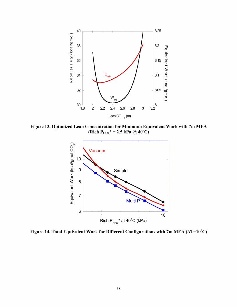
The optimization of the lean loading in a simple stripper using 7m MEA for a rich CO2 loading of 0.525 mol CO2/mol MEA (3.68 m) is shown in Figure 13. The minimum equivalent work (8.01 kcal/gmol CO2) occurs at a CO2 loading of 0.33 mol CO2 /mol MEA (2.39m) with a reboiler duty of 33.5 kcal/gmol CO2. The lean loading required to minimize reboiler duty does not coincide with that required to minimize equivalent work. The equilibrium partial pressure of CO2 in the rich solution leaving the absorber is 2.5 kPa. The lean partial pressure leaving the stripper bottom is 0.11 kPa at 40oC. This implies that greater than 90% removal can be achieved with the equivalent work minimized.

Figure 14 shows the minimum equivalent work for 7m MEA using the three configurations. The multipressure stripper gives the least equivalent work over the entire rich PCO2* range. The simple stripper is the least attractive configuration with the highest work over most of the rich PCO2* range. The multipressure stripper offers 8% energy savings when compared to the simple stripper. The vacuum stripper requires 6% less energy at high rich PCO2*.

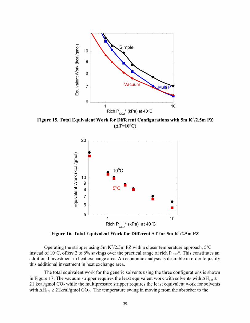
Figure 15 shows the minimum equivalent work for 5m K+/2.5m PZ using the three configurations. The vacuum stripper gives the least equivalent work over most of the rich PCO2* range with the multipressure stripper competitive at higher rich PCO2*. The simple stripper is the least attractive configuration at high rich PCO2*. In comparison to the simple stripper, the vacuum stripper requires 18% less energy at lower rich PCO2* and offers savings up to 8% at higher PCO2*.

The effect of varying the temperature approach in the cross exchanger was also studied.

38

30

32

34

36

38

40

8

8.05

8.1

8.15

8.2

8.25

1.8 2 2.2 2.4 2.6 2.8 3 3.2

Re

boile

r D

uty

(kc

al/g

mol

)E

quivale

nt W

ork (kca

l/gmo

l)

Lean CO2 (m)

Qreb

Weq

Figure 13. Optimized Lean Concentration for Minimum Equivalent Work with 7m MEA

(Rich PCO2* = 2.5 kPa @ 40oC)

6

7

8

9

10

1 10

Equ

ival

ent W

ork

(kca

l/gm

ol C

O2)

Rich PCO2

* at 40oC (kPa)

Simple

Multi P

Vacuum

Figure 14. Total Equivalent Work for Different Configurations with 7m MEA (∆T=10oC)

39

6

7

8

9

10

1 10

Equi

vale

nt W

ork

(kca

l/gm

ol)

Rich PCO2

* (kPa) at 40oC

Simple

VacuumMulti P

Figure 15. Total Equivalent Work for Different Configurations with 5m K+/2.5m PZ

(∆T=10oC)

5

6

789

10

20

1 10

Equi

vale

nt W

ork

(kca

l/gm

ol)

Rich PCO2

* (kPa) at 40oC

5oC

10oC

Figure 16. Total Equivalent Work for Different ∆T for 5m K+/2.5m PZ

Operating the stripper using 5m K+/2.5m PZ with a closer temperature approach, 5oC instead of 10oC, offers 2 to 6% savings over the practical range of rich PCO2*. This constitutes an additional investment in heat exchange area. An economic analysis is desirable in order to justify this additional investment in heat exchange area.

The total equivalent work for the generic solvents using the three configurations is shown in Figure 17. The vacuum stripper requires the least equivalent work with solvents with ∆Hdes ≤ 21 kcal/gmol CO2 while the multipressure stripper requires the least equivalent work for solvents with ∆Hdes ≥ 21kcal/gmol CO2. The temperature swing in moving from the absorber to the

40

stripper is only advantageous in reducing equivalent work for high ∆Hdes solvents. This result has some implications in solvent development.

1. For the simple configuration, any solvent with a heat of desorption less than that of 7m MEA (22 kcal/gmol CO2) will not minimize total equivalent work. This means that with the simple configuration, 7m MEA is perhaps the optimum solvent in terms of minimizing energy requirements.

2. In order to take advantage of the higher rates of 5m K+/2.5m PZ, vacuum stripping should be employed. Reducing the energy requirements for this solvent will involve the use of alternative process configurations.

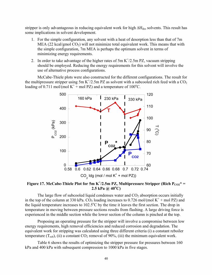
McCabe-Thiele plots were also constructed for the different configurations. The result for the multipressure stripper using 5m K+/2.5m PZ as solvent with a subcooled rich feed with a CO2 loading of 0.711 mol/(mol K+ + mol PZ) and a temperature of 100oC.

0

100

200

300

400

500

60

70

80

90

100

110

120

0.58 0.6 0.62 0.64 0.66 0.68 0.7 0.72 0.74

PC

O2 (k

Pa) T ( oC

)

CO2 ldg (mol / mol K+ + mol PZ))

PCO2

*

PCO2

T

160 kPa 230 kPa 330 kPa

Figure 17. McCabe-Thiele Plot for 5m K+/2.5m PZ, Multipressure Stripper (Rich PCO2* =

2.5 kPa @ 40oC) The large flow of subcooled liquid condenses water and CO2 absorption occurs initially

in the top of the column at 330 kPa. CO2 loading increases to 0.726 mol/(mol K+ + mol PZ) and the liquid temperature increases to 102.5oC by the time it leaves the first section. The drop in temperature in moving between pressure sections results from flashing. A large driving force is experienced in the middle section while the lower section of the column is pinched at the top.

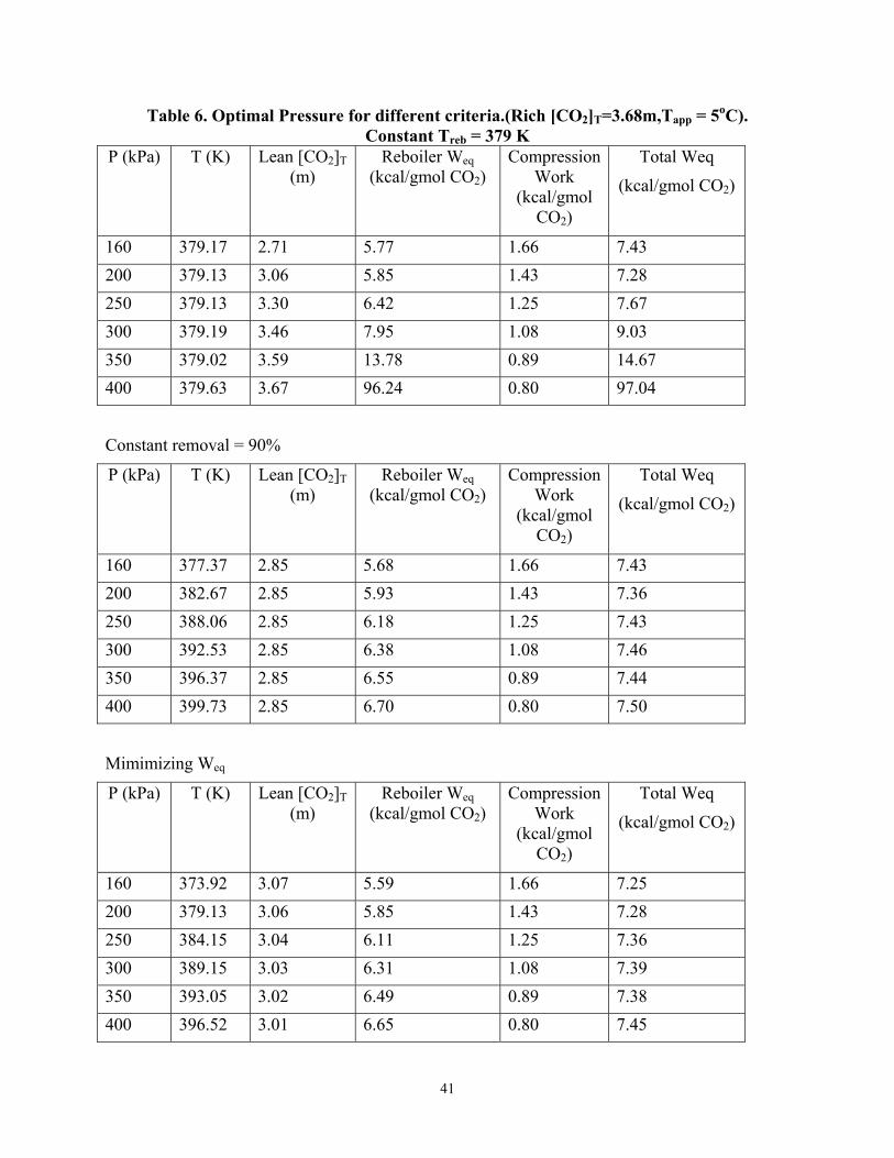
Proposing an operating pressure for the stripper will involve a compromise between low energy requirements, high removal efficiencies and reduced corrosion and degradation. The equivalent work for stripping was calculated using three different criteria (i) a constant reboiler temperature (Treb), (ii) a constant CO2 removal of 90%, (iii) the minimum equivalent work.

Table 6 shows the results of optimizing the stripper pressure for pressures between 160 kPa and 400 kPa with subsequent compression to 1000 kPa in five stages.

41

Table 6. Optimal Pressure for different criteria.(Rich [CO2]T=3.68m,Tapp = 5oC). Constant Treb = 379 K

P (kPa) T (K) Lean [CO2]T (m)

Reboiler Weq (kcal/gmol CO2)

Compression Work

(kcal/gmol CO2)

Total Weq

(kcal/gmol CO2)

160 379.17 2.71 5.77 1.66 7.43 200 379.13 3.06 5.85 1.43 7.28 250 379.13 3.30 6.42 1.25 7.67 300 379.19 3.46 7.95 1.08 9.03 350 379.02 3.59 13.78 0.89 14.67 400 379.63 3.67 96.24 0.80 97.04

Constant removal = 90%

P (kPa) T (K) Lean [CO2]T (m)

Reboiler Weq (kcal/gmol CO2)

Compression Work

(kcal/gmol CO2)

Total Weq

(kcal/gmol CO2)

160 377.37 2.85 5.68 1.66 7.43 200 382.67 2.85 5.93 1.43 7.36 250 388.06 2.85 6.18 1.25 7.43 300 392.53 2.85 6.38 1.08 7.46 350 396.37 2.85 6.55 0.89 7.44 400 399.73 2.85 6.70 0.80 7.50

Mimimizing Weq

P (kPa) T (K) Lean [CO2]T (m)

Reboiler Weq (kcal/gmol CO2)

Compression Work

(kcal/gmol CO2)

Total Weq

(kcal/gmol CO2)

160 373.92 3.07 5.59 1.66 7.25 200 379.13 3.06 5.85 1.43 7.28 250 384.15 3.04 6.11 1.25 7.36 300 389.15 3.03 6.31 1.08 7.39 350 393.05 3.02 6.49 0.89 7.38 400 396.52 3.01 6.65 0.80 7.45

42

The results show that at a constant Treb of 379 K, operating the stripper at a pressure greater than 180 kPa will result in less than 90% CO2 removal. In order to minimize the equivalent work with a Rich [CO2]T=3.68m, only 85% CO2 removal can be achieved.

Conclusions and Future Work

In this quarter, the ACM model was extended to model three configurations and three categories of solvents. The results show that the multipressure configuration is most attractive for 7m MEA over the entire range of PCO2*. The vacuum stripper is the most attractive for the 5m K+/2.5m PZ solvent. Since the vacuum stripper is operated at a lower temperature, alternative materials of construction like fiber-reinforced plastic can be used.

With generic solvents, the optimum ∆H is a function of the stripper configuration used. The vacuum stripper is favored for solvents with ∆Hdes ≤ 21 kcal/gmol CO2 while the multipressure configuration is attractive for solvents with ∆Hdes ≥ 21 kcal/gmol CO2 at a rich PCO2* = 2.5 kPa and rich absorber temperature of 40oC. Operating the cross exchanger at a 5oC approach instead of a 10oC approach offers 2-6% energy savings.

We are currently working on developing a mass transfer model. The results from this model will be presented in the next report. The results from our previous pilot plant campaigns are also been revisited to further understand the operation of the stripping column.

43

Subtask 1.10 – Simulate MEA Baseline by Ross Dugas

(Supported by this contract)

Summary

Since the last progress report the mass transfer data has been reviewed and an error has been corrected. The mass transfer coefficients reported in Figure 16 of the April-June DOE progress report have been increased by approximately 25%. The mass transfer data obtained from the MEA campaign has been compared to bench-scale measurements obtained by Dang (2000) as well as to Campaign 2 data using the 5mK+/2.5mPz solvent.

For both the Flexipac 1Y and IMTP #40 packings, one run with a high gas rate and one run with a low gas rate were chosen for Aspen simulations. The four runs compared the absorber performance of the simulation to the pilot plant by adjusting the height of the packing until a similar CO2 removal performance was obtained.

Results and Discussion

Mass transfer data obtained from the MEA pilot plant was compared to MEA bench-scale data as well as potassium carbonate/piperazine data from Campaign 2. In order to exclude pinch points from distorting the data, a driving factor was calculated. The driving factor is defined as the operating partial pressure of CO2 divided by the equilibrium partial pressure of CO2 at the same location in the column. The driving factor was calculated for both the top and bottom of the absorber. Driving factors lower than 1.5 were determined to be pinching and excluded from the mass transfer analysis. The Flexipac 1Y packing had 3 operating conditions excluded while the IMTP #40 had one. The comparison of the pilot plant’s mass transfer data to Dang’s wetted wall column data can be seen in Figure 18.

Figure 18 shows fairly good agreement for both the Flexipac 1Y and IMTP #40 with Dang’s mass transfer data. In calculating KG’s, the pilot plant average driving force was taken to be the average of the two driving forces at the ends of the absorber. The Flexipac 1Y was more likely to pinch at the temperature bulge so a greater scatter for Flexipac 1Y could be expected. The average loading for the pilot plant runs is the average of the absorber lean and rich solutions, a difference of up to 0.44 mol/mol. Dang’s data uses an average loading that differed by approximately 0.04 mol/mol due to the nature of the experiment.

Mass transfer characteristics have not yet been determined for each bed independently for the MEA campaign, so only mass transfer averages for the overall column have been shown in Figure 19. Figure 19 shows bench-scale and pilot plant mass transfer data for both the MEA and Pz/K2CO3 solvents.

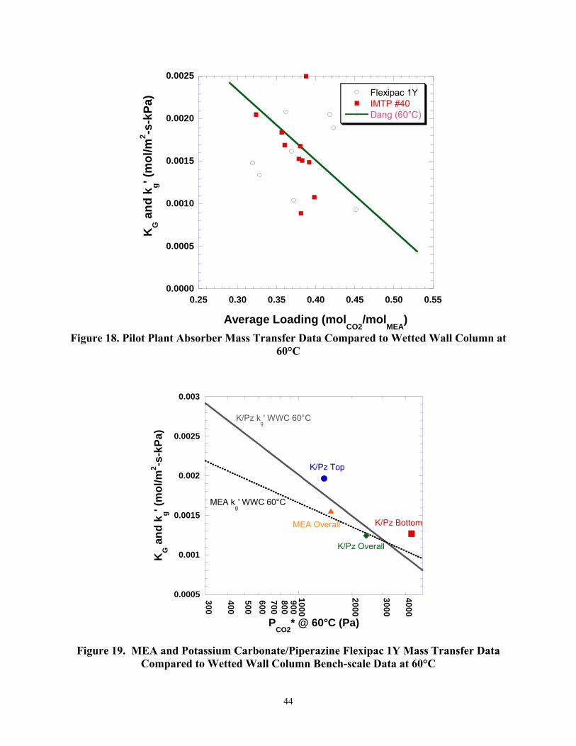
44

0.0000

0.0005

0.0010

0.0015

0.0020

0.0025

0.25 0.30 0.35 0.40 0.45 0.50 0.55

Flexipac 1YIMTP #40Dang (60°C)

KG a

nd k

g' (m

ol/m

2 -s-k

Pa)

Average Loading (molCO2

/molMEA

)

Figure 18. Pilot Plant Absorber Mass Transfer Data Compared to Wetted Wall Column at 60°C

0.0005

0.001

0.0015

0.002

0.0025

0.003

300

400

500600700800900

1000

2000

3000

4000K

G a

nd k

g' (m

ol/m

2 -s-k

Pa)

PCO2

* @ 60°C (Pa)

MEA Overall

K/Pz Overall

K/Pz kg' WWC 60°C

MEA kg' WWC 60°C

K/Pz Top

K/Pz Bottom

Figure 19. MEA and Potassium Carbonate/Piperazine Flexipac 1Y Mass Transfer Data

Compared to Wetted Wall Column Bench-scale Data at 60°C

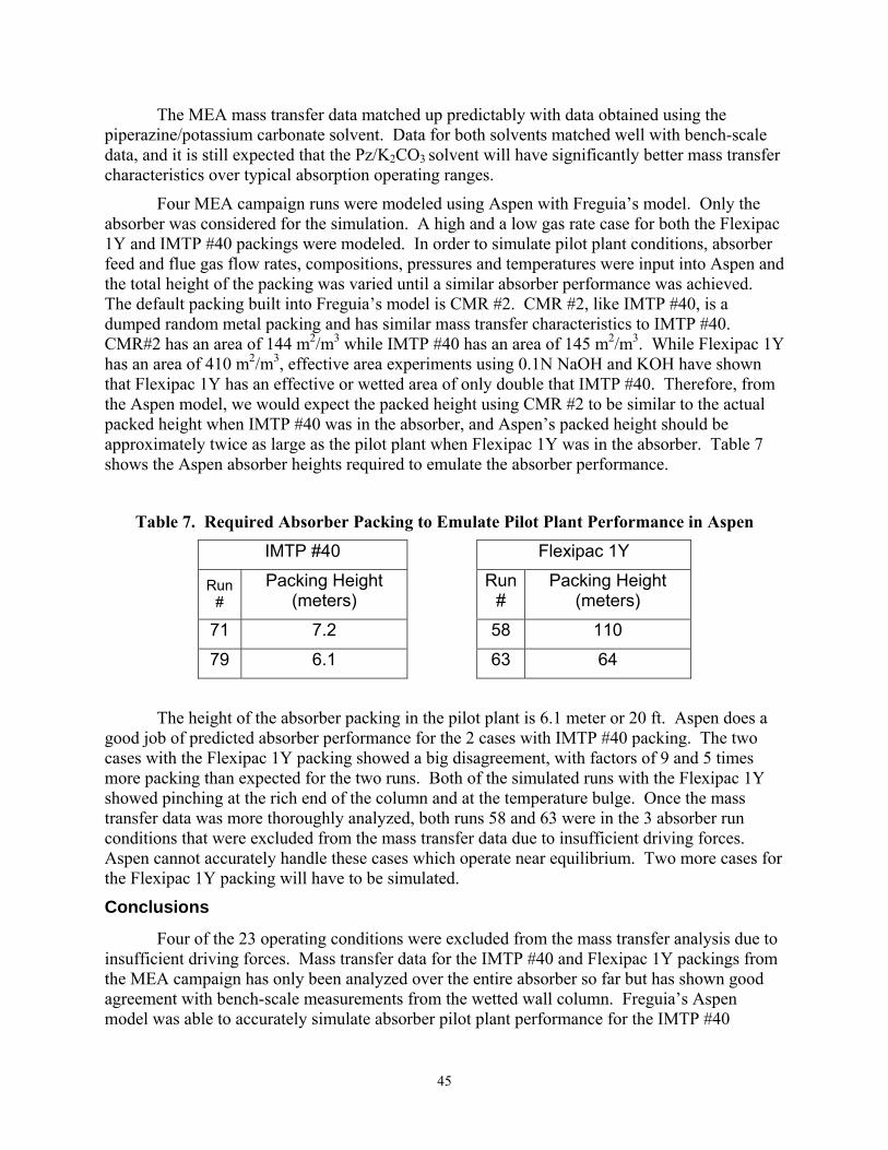
45

The MEA mass transfer data matched up predictably with data obtained using the piperazine/potassium carbonate solvent. Data for both solvents matched well with bench-scale data, and it is still expected that the Pz/K2CO3 solvent will have significantly better mass transfer characteristics over typical absorption operating ranges.

Four MEA campaign runs were modeled using Aspen with Freguia’s model. Only the absorber was considered for the simulation. A high and a low gas rate case for both the Flexipac 1Y and IMTP #40 packings were modeled. In order to simulate pilot plant conditions, absorber feed and flue gas flow rates, compositions, pressures and temperatures were input into Aspen and the total height of the packing was varied until a similar absorber performance was achieved. The default packing built into Freguia’s model is CMR #2. CMR #2, like IMTP #40, is a dumped random metal packing and has similar mass transfer characteristics to IMTP #40. CMR#2 has an area of 144 m2/m3 while IMTP #40 has an area of 145 m2/m3. While Flexipac 1Y has an area of 410 m2/m3, effective area experiments using 0.1N NaOH and KOH have shown that Flexipac 1Y has an effective or wetted area of only double that IMTP #40. Therefore, from the Aspen model, we would expect the packed height using CMR #2 to be similar to the actual packed height when IMTP #40 was in the absorber, and Aspen’s packed height should be approximately twice as large as the pilot plant when Flexipac 1Y was in the absorber. Table 7 shows the Aspen absorber heights required to emulate the absorber performance.

Table 7. Required Absorber Packing to Emulate Pilot Plant Performance in Aspen

IMTP #40 Flexipac 1Y

Run #

Packing Height (meters)

Run #

Packing Height (meters)

71 7.2 58 110

79 6.1 63 64

The height of the absorber packing in the pilot plant is 6.1 meter or 20 ft. Aspen does a good job of predicted absorber performance for the 2 cases with IMTP #40 packing. The two cases with the Flexipac 1Y packing showed a big disagreement, with factors of 9 and 5 times more packing than expected for the two runs. Both of the simulated runs with the Flexipac 1Y showed pinching at the rich end of the column and at the temperature bulge. Once the mass transfer data was more thoroughly analyzed, both runs 58 and 63 were in the 3 absorber run conditions that were excluded from the mass transfer data due to insufficient driving forces. Aspen cannot accurately handle these cases which operate near equilibrium. Two more cases for the Flexipac 1Y packing will have to be simulated.

Conclusions

Four of the 23 operating conditions were excluded from the mass transfer analysis due to insufficient driving forces. Mass transfer data for the IMTP #40 and Flexipac 1Y packings from the MEA campaign has only been analyzed over the entire absorber so far but has shown good agreement with bench-scale measurements from the wetted wall column. Freguia’s Aspen model was able to accurately simulate absorber pilot plant performance for the IMTP #40

46

packing. The accuracy of the model when comparing to the Flexipac 1Y packing is still inconclusive since both runs are severely pinched.

Future Work

Mass transfer coefficients need to be calculated for each bed in the absorber. Thus far, they have only been calculated across the entire absorber. Mass transfer characteristics also need to be determined for the stripper. Two more cases with Flexipac 1Y in the absorber need to be simulated using Aspen since both cases have pinching at the temperature bulge and the rich end of the column. Aspen cases will also be analyzed for the stripper, both at 1.6 atmospheres and at vacuum, to see it’s accuracy with respect to mass transfer and heat consumption.

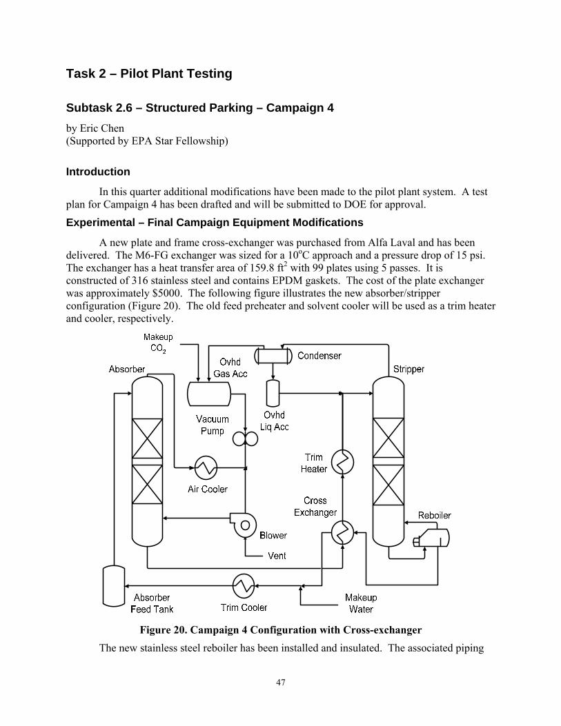
47

Task 2 – Pilot Plant Testing Subtask 2.6 – Structured Parking – Campaign 4 by Eric Chen (Supported by EPA Star Fellowship)

Introduction

In this quarter additional modifications have been made to the pilot plant system. A test plan for Campaign 4 has been drafted and will be submitted to DOE for approval.

Experimental – Final Campaign Equipment Modifications

A new plate and frame cross-exchanger was purchased from Alfa Laval and has been delivered. The M6-FG exchanger was sized for a 10oC approach and a pressure drop of 15 psi. The exchanger has a heat transfer area of 159.8 ft2 with 99 plates using 5 passes. It is constructed of 316 stainless steel and contains EPDM gaskets. The cost of the plate exchanger was approximately $5000. The following figure illustrates the new absorber/stripper configuration (Figure 20). The old feed preheater and solvent cooler will be used as a trim heater and cooler, respectively.

Figure 20. Campaign 4 Configuration with Cross-exchanger

The new stainless steel reboiler has been installed and insulated. The associated piping

48

has also been installed and insulated. The previous reboiler was made of carbon steel and may have recently developed pin sized holes and begun to leak.

An orifice plate will be installed on the cooling water of the air cooler instead of the proposed control valve to simplify plant operation. The cooling water will knock out most of the moisture from the absorber outlet gas stream to protect the downstream Vaisala CO2 probe. The condensate from the air cooler and the knockout filter will be drained to the absorber feed tank as before.

The inlet gas preheat (40oC) will come from steam generated by an existing 6-inch reboiler. Distillate from the stripper condensate will supply the water for the reboiler. The level in the reboiler will be maintained by adjusting the steam flow to the reboiler. The excess stripper condensate will be returned to the stripper as reflux. Approximately 0.6 gpm of water is needed to saturate the inlet absorber gas to 20% water at a gas flow rate of 500 cfm.

The new setup of the FTIR has been initiated and is nearing completion. The FTIR will be used measure CO2 and water concentration and piperazine volatility. Samples will be simultaneously withdrawn from the absorber inlet and outlet. Gas analysis will alternate between the two sample points via a three way valve located inside a heated box. Therefore, two 100 ft heated lines were procured from Environmental Supply Company. The heated lines consist of ¼ and 3/8-inch Teflon lines. The outside of the Teflon lines are covered with braided stainless. The heated lines have been installed outdoors and were attached to cable trays using plastic tie wraps. In addition, another sample pump and heater module was purchased from Air Quality Analytical, Inc.

The foaming issue encountered during the first two campaigns will be rectified by an activated carbon filter system. The system has been designed and the parts have been procured. The design was based on literature recommendations. Approximately 10-15% of the total lean solvent stream will be filtered, which should remove enough degradation products without removing the anti-foam. The carbon filter will be located downstream of the main lean solution bag filter. Another bag filter will be located downstream of the carbon filter to capture any charcoal fines. Two types of carbon will be used. Activated carbon from the filter manufacturer contains 10 x 50-mesh size activated carbon and is made of virgin coconut hulls. In addition, a lignite-based 8 x 30-mesh PETRODARCO activated carbon from NORIT will be tested. Four different filter bag materials (nomex, cotton, viscous rayon, and nylon) were tested because of material compatibility issues arising from the use of polypropylene in the previous campaigns. The filter materials were tested in warm solvent solutions and it was found that cotton performed the best based on visual inspections.

Experimental – Final Campaign Test Plan

In the fourth and final pilot plant campaign, experiments will be conducted with another structured packing, Flexipac 2Y HC (high capacity). The high capacity packing has a larger turning radius for the vapor flow, which reduces pressure drop and increases capacity. The new packing contains approximately 225 m2/m3 (68 ft2/ft3) of specific area, which is approximately half that of Flexipac 1Y (420 m2/m3). This should permit more utilization of the specific packing area and hence be more efficient and perhaps help with avoiding pinches. The absorber and stripper will each contain 20 ft of Flexipac 2Y, divided into 10 ft beds.

49

Two different solvent compositions will be tested in the last campaign. The first set of experiments will be conducted with the original 5mK+/2.5mPZ solvent. This will enable us characterize and compare the performance of the Flexipac 2Y HC to the Flexipac 1Y. A second set of experiments will be conducted with 6.4mK+/1.6mPZ. The second solvent composition has a heat of absorption that is about 50% lower and a capacity that is approximately 0-10% higher than that of the 5mK+/2.5mPZ. However, the CO2 absorption rate is about 40% less than the 5mK+/2.5mPZ solvent. Therefore, experiments with the second solvent composition should help establish the tradeoffs between fast CO2 absorption rates, low heat of absorption and higher capacity solvents.

In order to determine the absolute concentrations of the second solvent, solubility experiments were conducted with 4 different compositions: 6mK+/1.5mPZ, 6.4mK+/1.6mPZ, 6.8mK+/1.7mPZ, 7.2mK+/1.8mPZ. The ratio of potassium to piperazine was maintained at 4. Experiments conducted at 40, 50, and 60 oC and 4 different CO2 loadings for each solution. Higher piperazine and potassium concentrations result in faster absorption rates and larger solution capacities, respectively. However, as the concentration is increased, the risk of salting out the potassium bicarbonate or precipitating piperazine increases. The results are shown in Table 8.

At low CO2 loading, piperazine tends to form a separate layer from the potassium carbonate/bicarbonate solution. At rich CO2 loading, the potassium bicarbonate tends to salt out, precipitating as fine white crystals. The table shows that at 40oC, only the 6.4mK+/1.6mPZ solvent composition does not phase separate or form precipitates over the loading range that the pilot plant will be operated at. Therefore, this particular solvent composition was selected.

Finally, a detailed test plan for Campaign 4 has been prepared and will be submitted for approval.

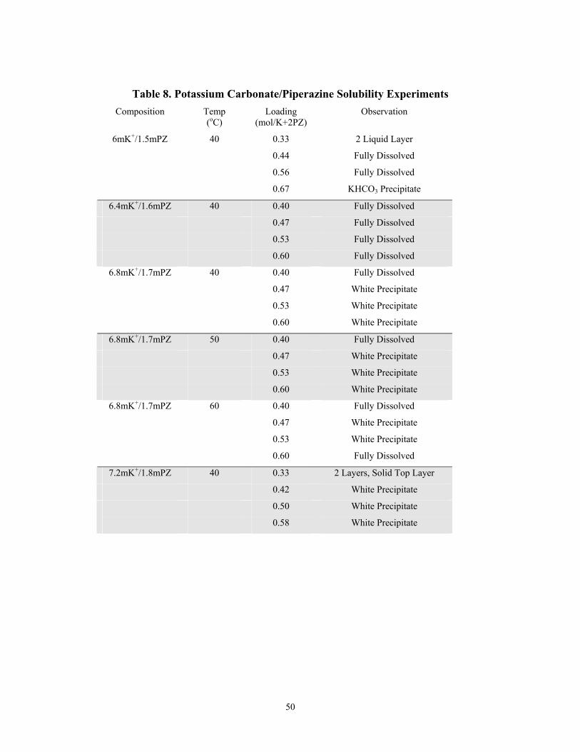
50

Table 8. Potassium Carbonate/Piperazine Solubility Experiments Composition Temp

(oC) Loading

(mol/K+2PZ) Observation

6mK+/1.5mPZ 40 0.33 2 Liquid Layer

0.44 Fully Dissolved

0.56 Fully Dissolved

0.67 KHCO3 Precipitate

6.4mK+/1.6mPZ 40 0.40 Fully Dissolved

0.47 Fully Dissolved

0.53 Fully Dissolved

0.60 Fully Dissolved

6.8mK+/1.7mPZ 40 0.40 Fully Dissolved

0.47 White Precipitate

0.53 White Precipitate

0.60 White Precipitate

6.8mK+/1.7mPZ 50 0.40 Fully Dissolved

0.47 White Precipitate

0.53 White Precipitate

0.60 White Precipitate

6.8mK+/1.7mPZ 60 0.40 Fully Dissolved

0.47 White Precipitate

0.53 White Precipitate

0.60 Fully Dissolved

7.2mK+/1.8mPZ 40 0.33 2 Layers, Solid Top Layer

0.42 White Precipitate

0.50 White Precipitate

0.58 White Precipitate

51

Task 3 – Solvent Losses Subtask 3.1 – Analysis of Degradation Products Andrew Sexton

(Supported by the Industrial Associates Program in CO2 Capture)

Introduction

This effort is the beginning of an extension of work by Goff on the oxidative degradation of MEA. Goff showed that oxidative degradation can be mass-transfer limited by the physical absorption of O2 into the amine and not by reaction kinetics. Goff also theorized that the oxidative degradation of MEA produced volatile ammonia as well as a host of other proposed degradation products. The major degradation products among these include formic acid, acetic acid, oxalic acid and glycolic acid. The oxygen stoichiometry necessary to produce these degradation products varies for each individual component; overall, it varies anywhere from 0.5 to 2.5 (Goff, 2004). Goff’s work on MEA degradation was limited to analyzing MEA degradation rates via the evolution of NH3. The ammonia evolution rates were measured using a Fourier Transform Infrared (FT-IR) analyzer.

This initial effort will extend gas-phase analysis by developing and applying various methods of liquid-phase analysis, specifically ion chromatography and nuclear magnetic resonance. These analytical methods will be used to quantify the rate of piperazine and MEA degradation as well as the rate of organic product formation.

The oxidative degradation of the amines may significantly affect the economics and environmental impact of these solvent systems. Oxidative degradation results in fragmentation of the amine solvent. The identity and quantity of degradation products is required to assess their impact on the environment and the process economics and to design for corrosion prevention and solvent reclaiming.

The current objectives for liquid-phase analysis include:

1. Verify that oxygen stoichiometry differs for systems using iron versus copper (both are currently added as corrosion inhibitors).

2. Confirm that NH3 evolution occurs in a 1:1 ratio with MEA degradation. 3. Once the stoichiometries are verified for each of the degradation products, expand the

oxygen physical absorption model and predict oxidation rates for a broader range of amine solvents (i.e. piperazine and piperazine/MEA blended systems).

Experimental

As stated in the July 2005 quarterly report, ion chromatography is the most extensively used liquid-phase analytical method at this point. Anion chromatography utilizes an AS11 IonPac column made by Dionex, located in the civil engineering building. The column operates as a miniature adsorption tower. An unknown solution is injected into the column. An eluent of sodium hydroxide is continuously passed through the column to flush the ions off the column and replenish it with hydroxide ions.

The ions leave the column and then pass through a suppressor, which provides a steady supply of

52

H+ ions. As a result, all other cations are flushed out of the system as waste, leaving a weakly ionized solution of H+ ions and the unknown anion(s) in water. This solution is passed through a conductivity meter, which provides a signal dependent upon the concentration of the anion in solution (Wang, 2005). Refer to the July 2005 quarterly report for a detailed description of the method.

The cation chromatograph, located in the CPE building, operates in a similar manner. It utilizes a CS16 IonPac column manufactured by Dionex; it is a packed column containing a divinylbenzene/ethylvinylbenzene resin that separates cations based on their affinity for the resin. The eluent is methanesulfonic acid, or MSA (CH3SO3H), and the suppressor produces a steady supply of OH- ions to flush out all other anions. The end result is a weakly ionized solution of the unknown cation and OH- ions in water (Dionex, 2005). The anion IC is being used to quantify rates of organic acid formation, while the cation IC is primarily for characterizing the rate of MEA degradation.

Nuclear magnetic resonance, or NMR, identifies unique 1H atoms and/or 13C atoms based on structure (double/triple bonds, attachment to acid/amine/etc. groups). Sealed liquid samples are subjected to a magnetic pulse, and each unique atom is characterized by a “chemical shift” on the readout. If the structure(s) in the solution is unknown, it may be necessary to construct a 2-D carbon-hydrogen correlation in order to determine structure. Samples must be prepared with approximately 10% D2O (by weight) and DSS (Shoulders, 2005). D2O, or deuterium oxide, is heavier than water and enhances the signal, thereby making the analysis easier. DSS, or Sodium 2,2-Dimethyl-2-Silapentane-5-Sulfonate, is used as a reference peak for aqueous solutions containing organic materials.

Results

Nuclear Magnetic Resonance (NMR)

In the previous report the location of formate, acetate, glycolate, and oxalate via NMR was hypothesized in experimental samples. This hypothesis was tested by preparing solutions of 7 molal MEA (unloaded) containing a rich amount of one of the organic acids (1 molar) and a lean amount of the other three organic acids (0.2 molar). Four solutions were prepared so that there was a rich solution for each of the organic acids. A baseline solution of 0.2 molar of each of the organic acids was prepared as well to give a reference point. Thus, an increase in magnitude of one of the peaks relative to the baseline scan identified that peak(s) as that particular organic acid product. The results of these scans are demonstrated in Figures 21 through 24.

From these scans, formate, glycolate, and acetate are readily identified using 1H NMR analysis; these three degradation products plus oxalate are identified from 13C. Oxalate does not show up on proton NMR analysis because of its structure; there are no hydrogen atoms on adjacent carbon atoms – they only appear on the hydroxide groups. Analysis of the experimentally degraded samples shows that these degradation products are present in appreciable amounts.

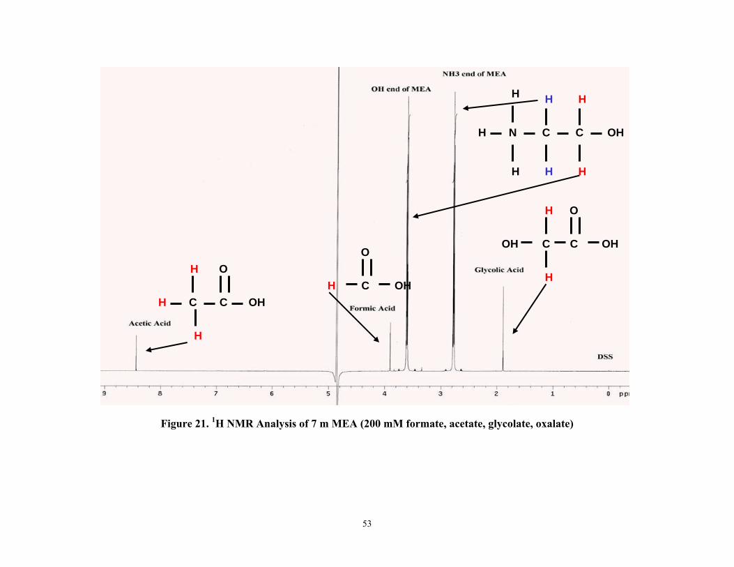
53

Figure 21. 1H NMR Analysis of 7 m MEA (200 mM formate, acetate, glycolate, oxalate)

C C OH

O

H

H

H C OH

O

H

C OH

O

C OH

H

H

OH C C N

H

H

H

H

H

H

H

54

Figure 22. 1H NMR Analysis of Sexton 12/14/04 (7 m MEA, 55 oC, α = 0.40, 0.2 mM Cu, 1400 RPM)

Acetate Formate

Glycolate

DSS

NH3 end of MEACOO-

OH end of MEACOO-

OH end of MEA NH3 end of

MEA

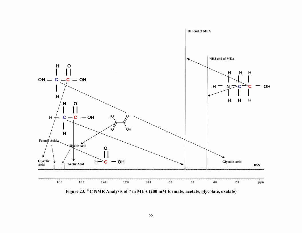
55

Figure 23. 13C NMR Analysis of 7 m MEA (200 mM formate, acetate, glycolate, oxalate)

C C OH

O

H

H

H

C OH

O

C OH

H

H

OH C C N

H

H

H

H

H

H

H

C OH

O

H

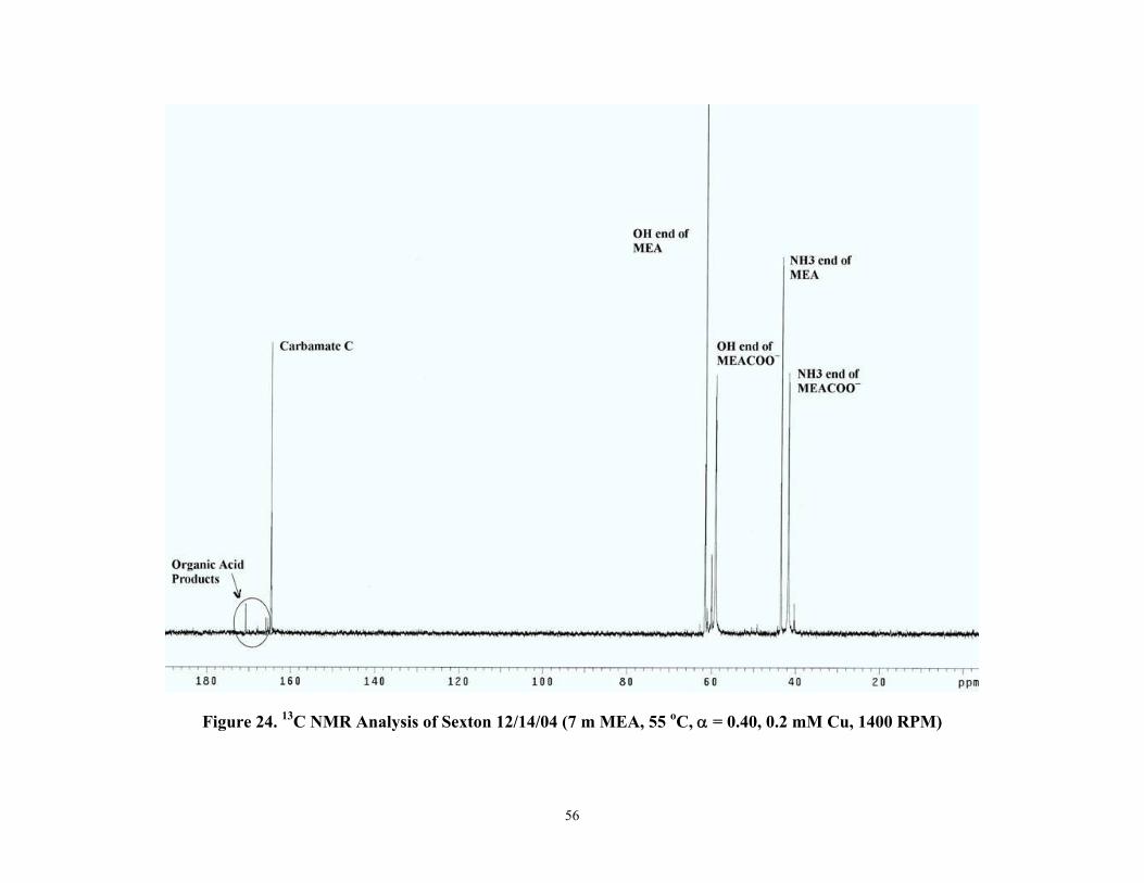
56

Figure 24. 13C NMR Analysis of Sexton 12/14/04 (7 m MEA, 55 oC, α = 0.40, 0.2 mM Cu, 1400 RPM)

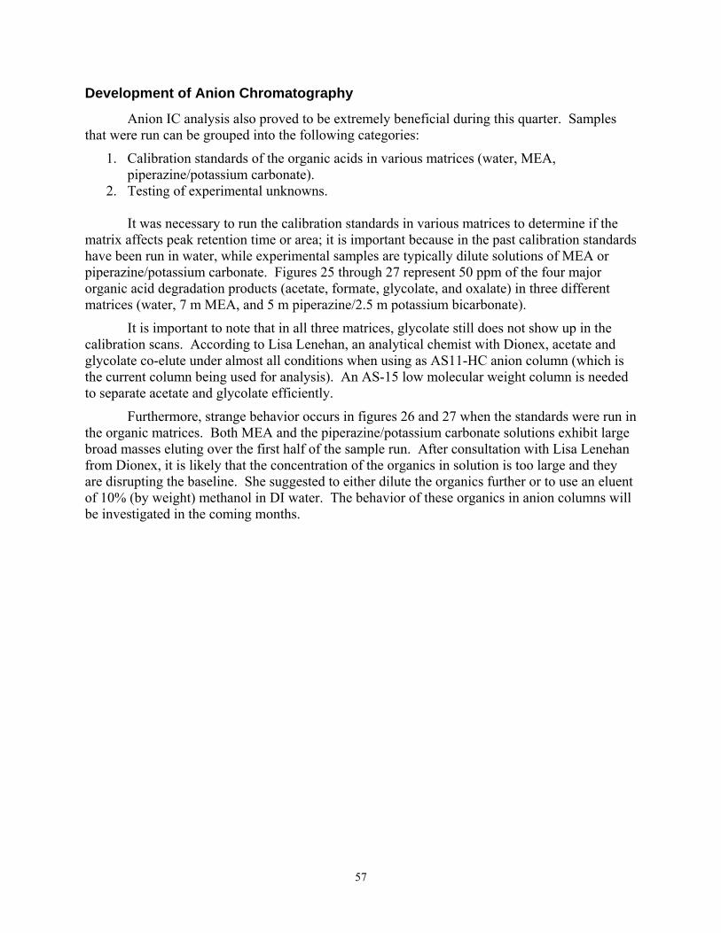
57

Development of Anion Chromatography

Anion IC analysis also proved to be extremely beneficial during this quarter. Samples that were run can be grouped into the following categories:

1. Calibration standards of the organic acids in various matrices (water, MEA, piperazine/potassium carbonate).

2. Testing of experimental unknowns. It was necessary to run the calibration standards in various matrices to determine if the

matrix affects peak retention time or area; it is important because in the past calibration standards have been run in water, while experimental samples are typically dilute solutions of MEA or piperazine/potassium carbonate. Figures 25 through 27 represent 50 ppm of the four major organic acid degradation products (acetate, formate, glycolate, and oxalate) in three different matrices (water, 7 m MEA, and 5 m piperazine/2.5 m potassium bicarbonate).

It is important to note that in all three matrices, glycolate still does not show up in the calibration scans. According to Lisa Lenehan, an analytical chemist with Dionex, acetate and glycolate co-elute under almost all conditions when using as AS11-HC anion column (which is the current column being used for analysis). An AS-15 low molecular weight column is needed to separate acetate and glycolate efficiently.

Furthermore, strange behavior occurs in figures 26 and 27 when the standards were run in the organic matrices. Both MEA and the piperazine/potassium carbonate solutions exhibit large broad masses eluting over the first half of the sample run. After consultation with Lisa Lenehan from Dionex, it is likely that the concentration of the organics in solution is too large and they are disrupting the baseline. She suggested to either dilute the organics further or to use an eluent of 10% (by weight) methanol in DI water. The behavior of these organics in anion columns will be investigated in the coming months.

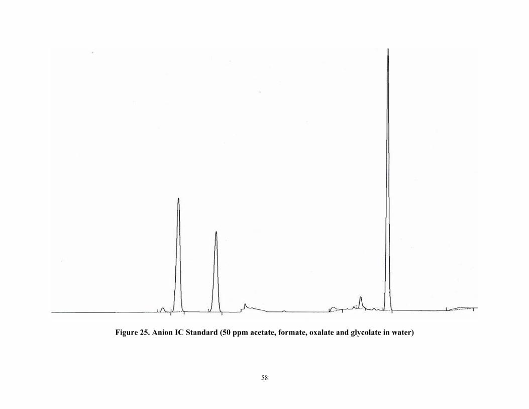
58

Figure 25. Anion IC Standard (50 ppm acetate, formate, oxalate and glycolate in water)

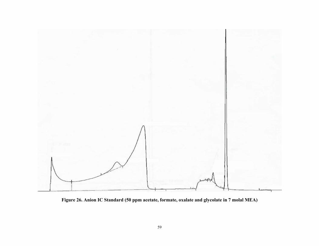
59

Figure 26. Anion IC Standard (50 ppm acetate, formate, oxalate and glycolate in 7 molal MEA)

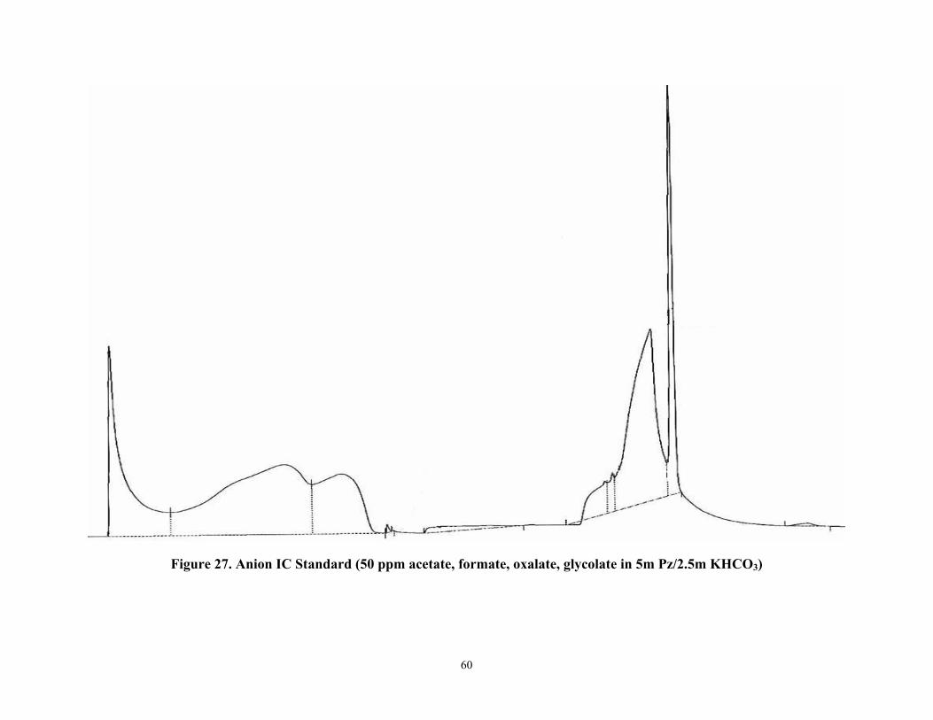
60

Figure 27. Anion IC Standard (50 ppm acetate, formate, oxalate, glycolate in 5m Pz/2.5m KHCO3)

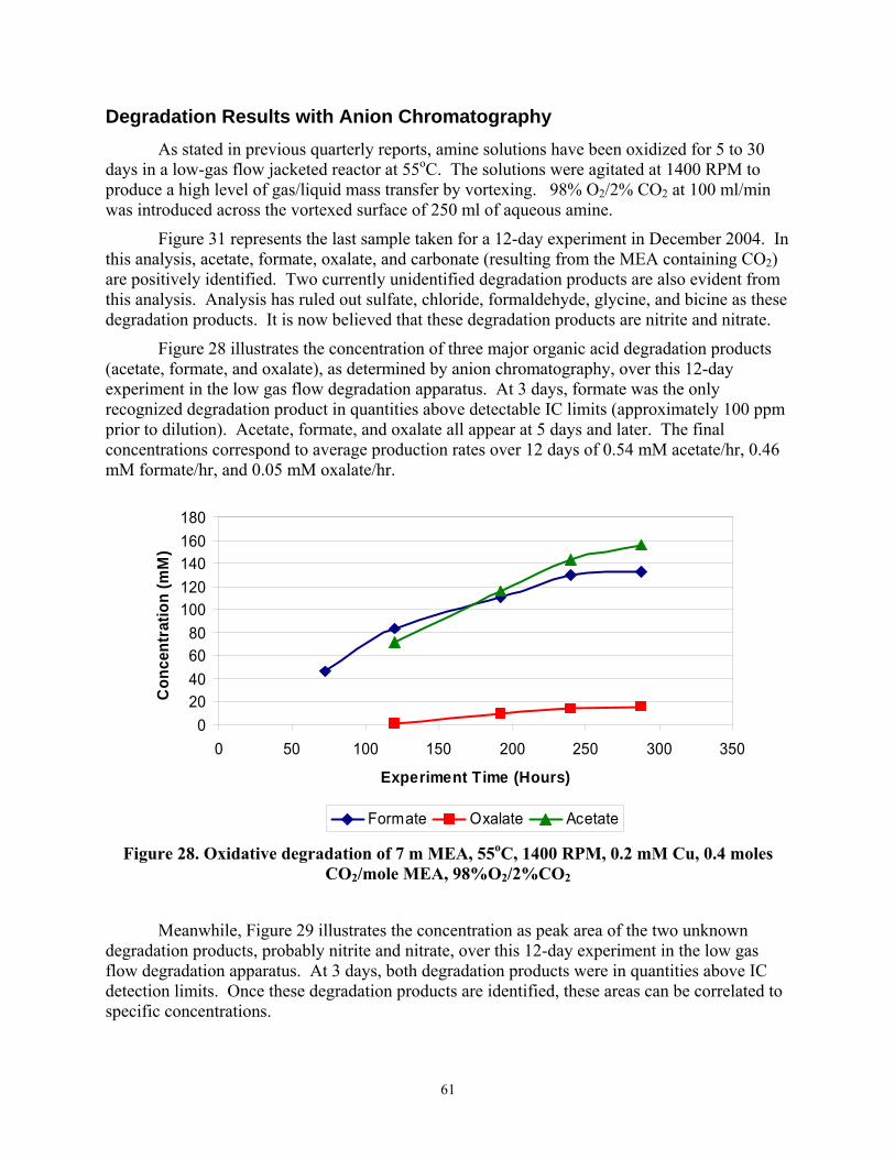
61

Degradation Results with Anion Chromatography As stated in previous quarterly reports, amine solutions have been oxidized for 5 to 30

days in a low-gas flow jacketed reactor at 55oC. The solutions were agitated at 1400 RPM to produce a high level of gas/liquid mass transfer by vortexing. 98% O2/2% CO2 at 100 ml/min was introduced across the vortexed surface of 250 ml of aqueous amine.

Figure 31 represents the last sample taken for a 12-day experiment in December 2004. In this analysis, acetate, formate, oxalate, and carbonate (resulting from the MEA containing CO2) are positively identified. Two currently unidentified degradation products are also evident from this analysis. Analysis has ruled out sulfate, chloride, formaldehyde, glycine, and bicine as these degradation products. It is now believed that these degradation products are nitrite and nitrate.

Figure 28 illustrates the concentration of three major organic acid degradation products (acetate, formate, and oxalate), as determined by anion chromatography, over this 12-day experiment in the low gas flow degradation apparatus. At 3 days, formate was the only recognized degradation product in quantities above detectable IC limits (approximately 100 ppm prior to dilution). Acetate, formate, and oxalate all appear at 5 days and later. The final concentrations correspond to average production rates over 12 days of 0.54 mM acetate/hr, 0.46 mM formate/hr, and 0.05 mM oxalate/hr.

020406080

100120140160180

0 50 100 150 200 250 300 350

Experiment Time (Hours)

Con

cent

ratio

n (m

M)

Formate Oxalate Acetate

Figure 28. Oxidative degradation of 7 m MEA, 55oC, 1400 RPM, 0.2 mM Cu, 0.4 moles CO2/mole MEA, 98%O2/2%CO2

Meanwhile, Figure 29 illustrates the concentration as peak area of the two unknown degradation products, probably nitrite and nitrate, over this 12-day experiment in the low gas flow degradation apparatus. At 3 days, both degradation products were in quantities above IC detection limits. Once these degradation products are identified, these areas can be correlated to specific concentrations.

62

0

1

2

3

4

0 50 100 150 200 250 300

Experiment Time (Hours)

Are

a ( µ

s*m

in)

Nitrite Nitrate

Figure 29. Oxidative degradation of 7 m MEA, 55oC, 1400 RPM, 0.2 mM Cu, 0.4 moles CO2/mole MEA, 98%O2/2%CO2

As detailed in the July 2005 quarterly report, experiments lasting 8 to 16 hours were

performed in the high gas flow degradation apparatus developed by Goff (2005). 250 ml of aqueous amine was sparged in a highly agitated reactor with 5 L/min of 2% CO2 in air. The offgas was continuously analyzed for ammonia and other volatile products by the FTIR at 180oC. The degradation inhibitor “A” was successively added so that the degradation products accumulated over a range of concentrations of the inhibitor, as shown in Figure 30. Acetate, formate, and oxalate formation rates were determined from liquid-phase analysis via anion chromatography; an average ammonia formation rate was calculated from gas-phase data collected and analyzed by the FTIR. These rates are shown in Table 9.

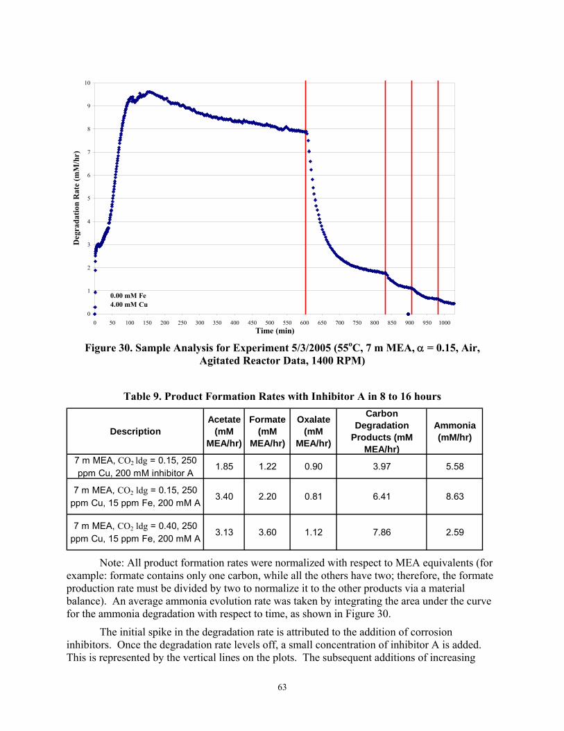
63

0

1

2

3

4

5

6

7

8

9

10

0 50 100 150 200 250 300 350 400 450 500 550 600 650 700 750 800 850 900 950 1000Time (min)

Deg

rada

tion

Rat

e (m

M/h

r)

0.00 mM Fe4.00 mM Cu

Figure 30. Sample Analysis for Experiment 5/3/2005 (55oC, 7 m MEA, α = 0.15, Air,

Agitated Reactor Data, 1400 RPM)

Table 9. Product Formation Rates with Inhibitor A in 8 to 16 hours

DescriptionAcetate

(mM MEA/hr)

Formate (mM

MEA/hr)

Oxalate (mM

MEA/hr)

Carbon Degradation

Products (mM MEA/hr)

Ammonia (mM/hr)

7 m MEA, CO2 ldg = 0.15, 250 ppm Cu, 200 mM inhibitor A

1.85 1.22 0.90 3.97 5.58

7 m MEA, CO2 ldg = 0.15, 250 ppm Cu, 15 ppm Fe, 200 mM A

3.40 2.20 0.81 6.41 8.63

7 m MEA, CO2 ldg = 0.40, 250 ppm Cu, 15 ppm Fe, 200 mM A

3.13 3.60 1.12 7.86 2.59

Note: All product formation rates were normalized with respect to MEA equivalents (for example: formate contains only one carbon, while all the others have two; therefore, the formate production rate must be divided by two to normalize it to the other products via a material balance). An average ammonia evolution rate was taken by integrating the area under the curve for the ammonia degradation with respect to time, as shown in Figure 30.

The initial spike in the degradation rate is attributed to the addition of corrosion inhibitors. Once the degradation rate levels off, a small concentration of inhibitor A is added. This is represented by the vertical lines on the plots. The subsequent additions of increasing

64

amounts of inhibitor A correlate to the decreasing degradation rates.

A brief analysis of Table 9 shows that carbon-containing degradation products (acetate, formate, and oxalate) are produced at lower rates than ammonia, a nitrogen-containing degradation product, at a lean loading of 0.15. At a rich loading of 0.4, this trend is reversed. These trends cannot be verified until the analysis of these samples is replicated and it is determined whether glycolate, nitrate, and nitrite are significant degradation products. However, this analysis does suggest the degradation stoichiometry differs at lean and rich loadings.

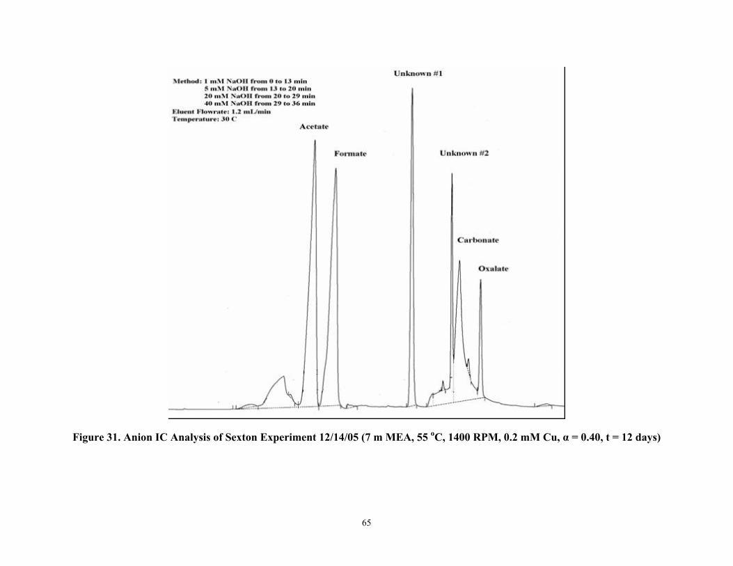
65

Figure 31. Anion IC Analysis of Sexton Experiment 12/14/05 (7 m MEA, 55 oC, 1400 RPM, 0.2 mM Cu, α = 0.40, t = 12 days)

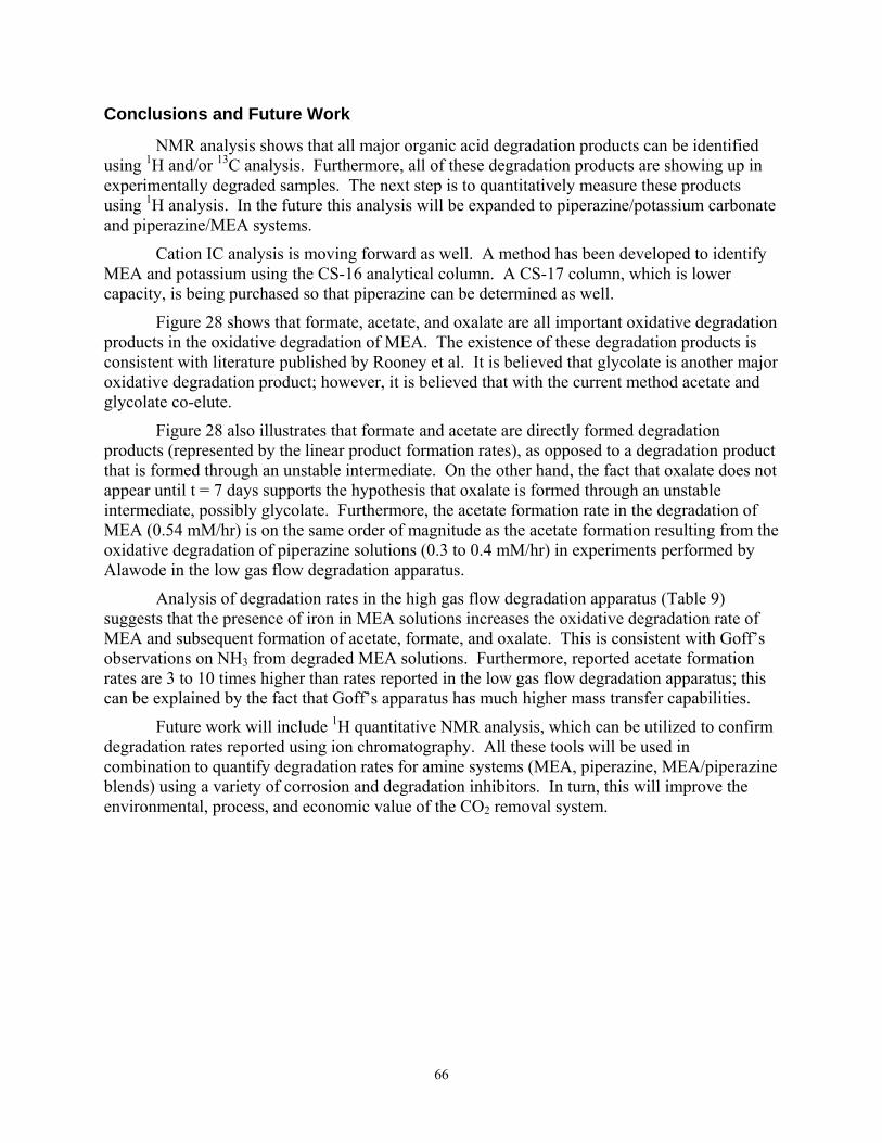
66

Conclusions and Future Work

NMR analysis shows that all major organic acid degradation products can be identified using 1H and/or 13C analysis. Furthermore, all of these degradation products are showing up in experimentally degraded samples. The next step is to quantitatively measure these products using 1H analysis. In the future this analysis will be expanded to piperazine/potassium carbonate and piperazine/MEA systems.

Cation IC analysis is moving forward as well. A method has been developed to identify MEA and potassium using the CS-16 analytical column. A CS-17 column, which is lower capacity, is being purchased so that piperazine can be determined as well.

Figure 28 shows that formate, acetate, and oxalate are all important oxidative degradation products in the oxidative degradation of MEA. The existence of these degradation products is consistent with literature published by Rooney et al. It is believed that glycolate is another major oxidative degradation product; however, it is believed that with the current method acetate and glycolate co-elute.

Figure 28 also illustrates that formate and acetate are directly formed degradation products (represented by the linear product formation rates), as opposed to a degradation product that is formed through an unstable intermediate. On the other hand, the fact that oxalate does not appear until t = 7 days supports the hypothesis that oxalate is formed through an unstable intermediate, possibly glycolate. Furthermore, the acetate formation rate in the degradation of MEA (0.54 mM/hr) is on the same order of magnitude as the acetate formation resulting from the oxidative degradation of piperazine solutions (0.3 to 0.4 mM/hr) in experiments performed by Alawode in the low gas flow degradation apparatus.

Analysis of degradation rates in the high gas flow degradation apparatus (Table 9) suggests that the presence of iron in MEA solutions increases the oxidative degradation rate of MEA and subsequent formation of acetate, formate, and oxalate. This is consistent with Goff’s observations on NH3 from degraded MEA solutions. Furthermore, reported acetate formation rates are 3 to 10 times higher than rates reported in the low gas flow degradation apparatus; this can be explained by the fact that Goff’s apparatus has much higher mass transfer capabilities.

Future work will include 1H quantitative NMR analysis, which can be utilized to confirm degradation rates reported using ion chromatography. All these tools will be used in combination to quantify degradation rates for amine systems (MEA, piperazine, MEA/piperazine blends) using a variety of corrosion and degradation inhibitors. In turn, this will improve the environmental, process, and economic value of the CO2 removal system.

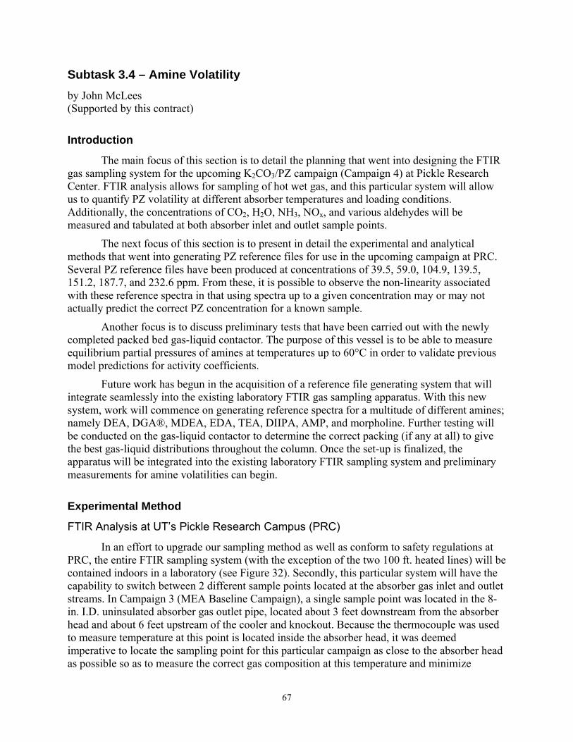
67

Subtask 3.4 – Amine Volatility by John McLees (Supported by this contract)

Introduction

The main focus of this section is to detail the planning that went into designing the FTIR gas sampling system for the upcoming K2CO3/PZ campaign (Campaign 4) at Pickle Research Center. FTIR analysis allows for sampling of hot wet gas, and this particular system will allow us to quantify PZ volatility at different absorber temperatures and loading conditions. Additionally, the concentrations of CO2, H2O, NH3, NOx, and various aldehydes will be measured and tabulated at both absorber inlet and outlet sample points.

The next focus of this section is to present in detail the experimental and analytical methods that went into generating PZ reference files for use in the upcoming campaign at PRC. Several PZ reference files have been produced at concentrations of 39.5, 59.0, 104.9, 139.5, 151.2, 187.7, and 232.6 ppm. From these, it is possible to observe the non-linearity associated with these reference spectra in that using spectra up to a given concentration may or may not actually predict the correct PZ concentration for a known sample.

Another focus is to discuss preliminary tests that have been carried out with the newly completed packed bed gas-liquid contactor. The purpose of this vessel is to be able to measure equilibrium partial pressures of amines at temperatures up to 60°C in order to validate previous model predictions for activity coefficients.

Future work has begun in the acquisition of a reference file generating system that will integrate seamlessly into the existing laboratory FTIR gas sampling apparatus. With this new system, work will commence on generating reference spectra for a multitude of different amines; namely DEA, DGA®, MDEA, EDA, TEA, DIIPA, AMP, and morpholine. Further testing will be conducted on the gas-liquid contactor to determine the correct packing (if any at all) to give the best gas-liquid distributions throughout the column. Once the set-up is finalized, the apparatus will be integrated into the existing laboratory FTIR sampling system and preliminary measurements for amine volatilities can begin.

Experimental Method

FTIR Analysis at UT’s Pickle Research Campus (PRC)

In an effort to upgrade our sampling method as well as conform to safety regulations at PRC, the entire FTIR sampling system (with the exception of the two 100 ft. heated lines) will be contained indoors in a laboratory (see Figure 32). Secondly, this particular system will have the capability to switch between 2 different sample points located at the absorber gas inlet and outlet streams. In Campaign 3 (MEA Baseline Campaign), a single sample point was located in the 8-in. I.D. uninsulated absorber gas outlet pipe, located about 3 feet downstream from the absorber head and about 6 feet upstream of the cooler and knockout. Because the thermocouple was used to measure temperature at this point is located inside the absorber head, it was deemed imperative to locate the sampling point for this particular campaign as close to the absorber head as possible so as to measure the correct gas composition at this temperature and minimize

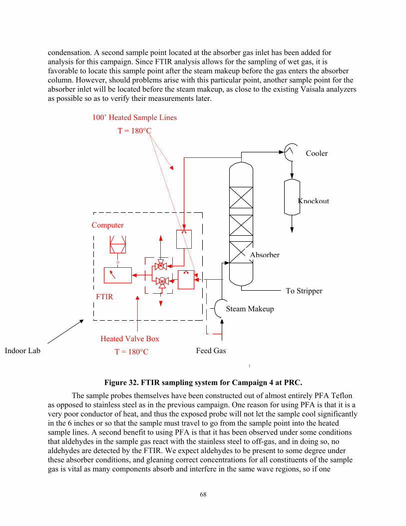
68

condensation. A second sample point located at the absorber gas inlet has been added for analysis for this campaign. Since FTIR analysis allows for the sampling of wet gas, it is favorable to locate this sample point after the steam makeup before the gas enters the absorber column. However, should problems arise with this particular point, another sample point for the absorber inlet will be located before the steam makeup, as close to the existing Vaisala analyzers as possible so as to verify their measurements later.

Figure 32. FTIR sampling system for Campaign 4 at PRC.

The sample probes themselves have been constructed out of almost entirely PFA Teflon as opposed to stainless steel as in the previous campaign. One reason for using PFA is that it is a very poor conductor of heat, and thus the exposed probe will not let the sample cool significantly in the 6 inches or so that the sample must travel to go from the sample point into the heated sample lines. A second benefit to using PFA is that it has been observed under some conditions that aldehydes in the sample gas react with the stainless steel to off-gas, and in doing so, no aldehydes are detected by the FTIR. We expect aldehydes to be present to some degree under these absorber conditions, and gleaning correct concentrations for all constituents of the sample gas is vital as many components absorb and interfere in the same wave regions, so if one

Feed Gas

Steam Makeup

To Stripper

Absorber

Knockout

Cooler

Indoor Lab Heated Valve Box

T = 180°C

FTIR

Computer

100’ Heated Sample Lines

T = 180°C

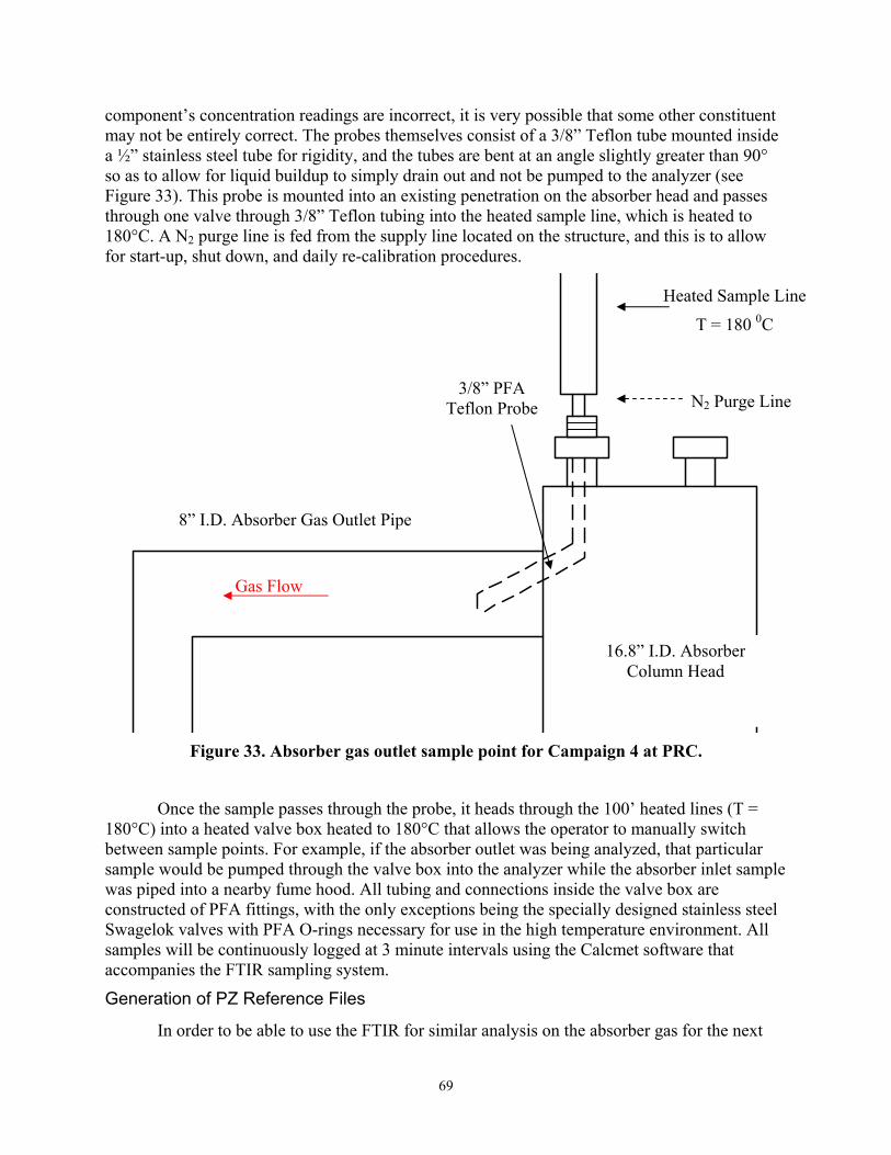
69

component’s concentration readings are incorrect, it is very possible that some other constituent may not be entirely correct. The probes themselves consist of a 3/8” Teflon tube mounted inside a ½” stainless steel tube for rigidity, and the tubes are bent at an angle slightly greater than 90° so as to allow for liquid buildup to simply drain out and not be pumped to the analyzer (see Figure 33). This probe is mounted into an existing penetration on the absorber head and passes through one valve through 3/8” Teflon tubing into the heated sample line, which is heated to 180°C. A N2 purge line is fed from the supply line located on the structure, and this is to allow for start-up, shut down, and daily re-calibration procedures.

Figure 33. Absorber gas outlet sample point for Campaign 4 at PRC.

Once the sample passes through the probe, it heads through the 100’ heated lines (T = 180°C) into a heated valve box heated to 180°C that allows the operator to manually switch between sample points. For example, if the absorber outlet was being analyzed, that particular sample would be pumped through the valve box into the analyzer while the absorber inlet sample was piped into a nearby fume hood. All tubing and connections inside the valve box are constructed of PFA fittings, with the only exceptions being the specially designed stainless steel Swagelok valves with PFA O-rings necessary for use in the high temperature environment. All samples will be continuously logged at 3 minute intervals using the Calcmet software that accompanies the FTIR sampling system.

Generation of PZ Reference Files

In order to be able to use the FTIR for similar analysis on the absorber gas for the next

8” I.D. Absorber Gas Outlet Pipe

3/8” PFA Teflon Probe

Heated Sample Line

T = 180 0C

Gas Flow

16.8” I.D. Absorber Column Head

N2 Purge Line

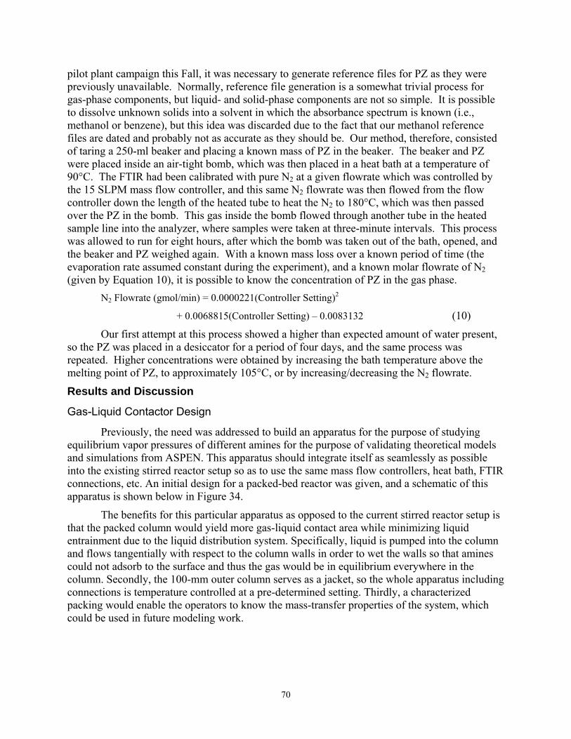
70

pilot plant campaign this Fall, it was necessary to generate reference files for PZ as they were previously unavailable. Normally, reference file generation is a somewhat trivial process for gas-phase components, but liquid- and solid-phase components are not so simple. It is possible to dissolve unknown solids into a solvent in which the absorbance spectrum is known (i.e., methanol or benzene), but this idea was discarded due to the fact that our methanol reference files are dated and probably not as accurate as they should be. Our method, therefore, consisted of taring a 250-ml beaker and placing a known mass of PZ in the beaker. The beaker and PZ were placed inside an air-tight bomb, which was then placed in a heat bath at a temperature of 90°C. The FTIR had been calibrated with pure N2 at a given flowrate which was controlled by the 15 SLPM mass flow controller, and this same N2 flowrate was then flowed from the flow controller down the length of the heated tube to heat the N2 to 180°C, which was then passed over the PZ in the bomb. This gas inside the bomb flowed through another tube in the heated sample line into the analyzer, where samples were taken at three-minute intervals. This process was allowed to run for eight hours, after which the bomb was taken out of the bath, opened, and the beaker and PZ weighed again. With a known mass loss over a known period of time (the evaporation rate assumed constant during the experiment), and a known molar flowrate of N2 (given by Equation 10), it is possible to know the concentration of PZ in the gas phase.

N2 Flowrate (gmol/min) = 0.0000221(Controller Setting)2

+ 0.0068815(Controller Setting) – 0.0083132 (10)

Our first attempt at this process showed a higher than expected amount of water present, so the PZ was placed in a desiccator for a period of four days, and the same process was repeated. Higher concentrations were obtained by increasing the bath temperature above the melting point of PZ, to approximately 105°C, or by increasing/decreasing the N2 flowrate.

Results and Discussion

Gas-Liquid Contactor Design

Previously, the need was addressed to build an apparatus for the purpose of studying equilibrium vapor pressures of different amines for the purpose of validating theoretical models and simulations from ASPEN. This apparatus should integrate itself as seamlessly as possible into the existing stirred reactor setup so as to use the same mass flow controllers, heat bath, FTIR connections, etc. An initial design for a packed-bed reactor was given, and a schematic of this apparatus is shown below in Figure 34.

The benefits for this particular apparatus as opposed to the current stirred reactor setup is that the packed column would yield more gas-liquid contact area while minimizing liquid entrainment due to the liquid distribution system. Specifically, liquid is pumped into the column and flows tangentially with respect to the column walls in order to wet the walls so that amines could not adsorb to the surface and thus the gas would be in equilibrium everywhere in the column. Secondly, the 100-mm outer column serves as a jacket, so the whole apparatus including connections is temperature controlled at a pre-determined setting. Thirdly, a characterized packing would enable the operators to know the mass-transfer properties of the system, which could be used in future modeling work.

71

Figure 34. Proposed laboratory scale packed column.

One initial problem faced after construction was the difficulty associated with inserting a packing support into the 70-mm column through the tapered 62-mm opening. To get around this, the apparatus was tested without a support, and thus packed to a height of 16” with 10 mm stainless steel Jaeger Interpack and tested with water and air. It was found that leveling the apparatus has a big effect on the gas and liquid distributions throughout the packing, and this is something that must be corrected when the system is to be put into regular use. Because the column was not exactly level, the gas flowed almost exclusively to the front of the column for the first 4 or 5 inches and then slowly bubbled out throughout the packing. Furthermore, at low liquid flowrates, the current tangential liquid distribution system failed to wet the center of the packing at the top, and the only way to wet the entire packing in this mode was to operate at 100% flooding. On the other hand, at higher liquid flowrates, the liquid actually splashed on impact with the column walls, creating a great deal of liquid entrainment. As a result, the packing was then dumped out, and the column was tested as a bubble column. This mode allowed for significantly better gas-liquid distribution as well as more area for mass transfer, but perhaps the greatest benefit is its simplicity as compared to either the stirred reactor or packed

Heating Fluid In

Heating Fluid Out

Liquid Out Gas In

Liquid In

Gas Out (to FTIR)Temperature In

100-mm I.D.

70-mm I.D. 12”

4” Packing Support

72

column. The bubble column would be preferable to the stirred reactor because it has far less liquid entrainment, and has at least if not more gas-liquid contact area for mass transfer. The bubble column seems better than the packed column in that the gas-liquid distribution appears more uniform without the packing, and thus there is no need to worry about a fraction of the column that is not being used for mass transfer as with the packed column configuration.

It appears for now that the bubble column would be the better choice if the liquid distribution system were to go unchanged; however, a wall wiper could be added to aid in distributing the liquid to the middle of the packing at the top of the column if the packed bed setup was to be used. However, it may be more practical to continue to operate the vessel as a bubble column. In that case, it may be worthwhile to consider a gas distributor at the bottom of the column to help create a uniform gas dispersion.

PZ Method Development

PZ reference files were produced for concentrations of 2.4, 39.5, 59, 104.9, 139.5, 151.2, 187.7, and 232.6 ppm, and these spectra will be added to the analysis package for the FTIR software for the upcoming K2CO3/PZ campaign. These files were tested for linearity by checking each file individually against a known sample and comparing the accuracy with which that file predicted the sample’s composition. For example, if the 2.4 ppm reference file predicted a known sample of 100 ppm PZ to be 100 ppm, and then a 100 ppm reference file predicted a 2.4 ppm sample to be exactly 2.4 ppm, then the spectra would be linear between these regions. It was seen that for PZ samples, however, that the peaks are very non-linear in nature, so it is critical to have a broad range of concentrations in order to accurate quantify PZ volatility. Two reference files at higher concentrations (407 and 470.9 ppm) have been produced and their linearity is being tested at this time.

Future Work

PZ volatilities from the upcoming Campaign 4 at PRC will be calculated at the conclusion of the experiment and compared to previous model predictions. Furthermore, concentrations for CO2, H2O, NH3, NOx, and various aldehydes will be tabulated at both absorber gas inlet and outlet sample points. Further testing and modifications to the laboratory-scale gas-liquid contactor will continue until the apparatus appears ready for experimentation. At this point, the mass transfer properties will be characterized by a known experiment such as absorption of SO2 by NaOH. Once these are known, equilibrium partial pressures of MEA and PZ can be obtained at various temperatures and loadings in a controlled laboratory setting. Lastly, a reference file generation system has been purchased, and this will allow us to calibrate the FTIR for several amines such as DEA, DGA®, MDEA, EDA, TEA, DIIPA, AMP, and morpholine. Once these reference spectra have been generated, these amines can be studied in the gas-liquid contactor and their respective volatilities can be measured.

73

Task 4 – Solvent Reclaiming Subtask 4.2 – Liquid/Liquid Equilibrium By Daniel Ellenberger

Supported by the Industrial Associates Program

Introduction

In order to ensure that a solution will not salt out or precipitate while running the pilot plant, experiments were performed to determine solubility limits for the desired concentrations. In Campaign 4, the pilot plant will use a solvent composition at K+/PZ =4 at a temperature as low as 40°C.

Apparatus

The apparatus for the solubility experiment is a constant temperature bath mounted above a stir plate so that the samples can effectively agitated at a constant temperature. The container is a clear acrylic box made by Fischer Scientific. The box can support bath temperatures up to 70°C. The bath is filled with tap water. A water circulator is mounted on top of the box and set up so that it can maintain the bath at a constant temperature. The entire bath unit is raised up off of the laboratory bench so that a magnetic stirrer can operate underneath it. A magnetic stir bar is placed into each solution. The stirrer is set to provide a slow agitation to the samples so that they precipitate instead of becoming supersaturated.

Procedure

The samples were prepared in 50mL Erlenmeyer flasks at a four to one ratio of K+ to Pz. The K+ concentrations were 6.0 m, 6.4 m, and 6.8 m. The CO2 concentration was varied over a range of loading by varying the amounts of potassium carbonate and potassium bicarbonate. The source of the potassium carbonate and bicarbonate was Fischer Scientific. The piperazine was obtained from Acros Organics.

The first batch at 6.0 m K+ showed that precipitation at 40°C occurred with solutions prepared at the extreme CO2 loading of just potassium carbonate or just potassium bicarbonate. Therefore, measurements at the other K+ concentrations were made with mixtures of potassium carbonate and potassium bicarbonate.

Each sample was heated while the components dissolved until it reached a temperature at which the components became fully dissolved and a clear solution was obtained. A magnetic stir bar was placed in the flask and the solution was agitated during the heating. The flask was then capped with a rubber stopper and placed into the temperature bath. The samples were left to equilibrate in the bath for a period of at least two hours. During the equilibration period, the stir bar was allowed to rotate freely within the solution to make sure that the solution was adequately mixed. The samples were then examined for any phase separation.

The final concentration of samples, 6.8 m K+, was heated to 60°C to see if the any of the precipitated solutions would dissolve. The samples were allowed to equilibrate for at least two hours again. After observations were made, the temperature of the bath was lowered to observe any precipitation at 50°C. Once the solutions have equilibrated, observations of the contents

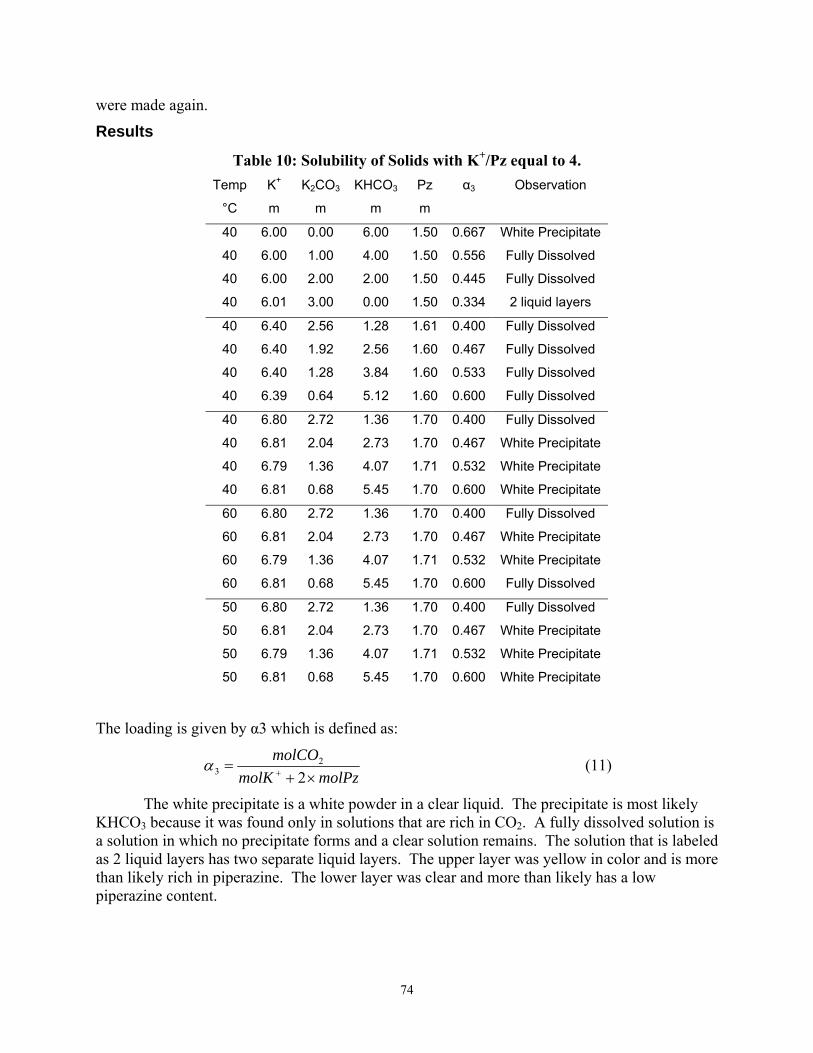
74

were made again.

Results

Table 10: Solubility of Solids with K+/Pz equal to 4. Temp K+ K2CO3 KHCO3 Pz α3 Observation

°C m m m m

40 6.00 0.00 6.00 1.50 0.667 White Precipitate

40 6.00 1.00 4.00 1.50 0.556 Fully Dissolved

40 6.00 2.00 2.00 1.50 0.445 Fully Dissolved

40 6.01 3.00 0.00 1.50 0.334 2 liquid layers

40 6.40 2.56 1.28 1.61 0.400 Fully Dissolved

40 6.40 1.92 2.56 1.60 0.467 Fully Dissolved

40 6.40 1.28 3.84 1.60 0.533 Fully Dissolved

40 6.39 0.64 5.12 1.60 0.600 Fully Dissolved

40 6.80 2.72 1.36 1.70 0.400 Fully Dissolved

40 6.81 2.04 2.73 1.70 0.467 White Precipitate

40 6.79 1.36 4.07 1.71 0.532 White Precipitate

40 6.81 0.68 5.45 1.70 0.600 White Precipitate

60 6.80 2.72 1.36 1.70 0.400 Fully Dissolved

60 6.81 2.04 2.73 1.70 0.467 White Precipitate

60 6.79 1.36 4.07 1.71 0.532 White Precipitate

60 6.81 0.68 5.45 1.70 0.600 Fully Dissolved

50 6.80 2.72 1.36 1.70 0.400 Fully Dissolved

50 6.81 2.04 2.73 1.70 0.467 White Precipitate

50 6.79 1.36 4.07 1.71 0.532 White Precipitate

50 6.81 0.68 5.45 1.70 0.600 White Precipitate

The loading is given by α3 which is defined as:

molPzmolKmolCO

×+= + 2

23α (11)

The white precipitate is a white powder in a clear liquid. The precipitate is most likely KHCO3 because it was found only in solutions that are rich in CO2. A fully dissolved solution is a solution in which no precipitate forms and a clear solution remains. The solution that is labeled as 2 liquid layers has two separate liquid layers. The upper layer was yellow in color and is more than likely rich in piperazine. The lower layer was clear and more than likely has a low piperazine content.

75

Conclusions

Samples of pure carbonate or pure bicarbonate ions will precipitate or phase separate more readily than solutions that are a mixture of the two ions. A solution that is rich in potassium carbonate seems to have a tendency to separate into two liquid layers. This is consistent with observations made by Cullinane (2005). Solutions that are rich in bicarbonate tend to precipitate out a white powder. Any methods run in a pilot must avoid being too rich or lean in loading to avoid multiple liquid layers or precipitation.

Another important conclusion is that a pilot plant run at 40°C and a K+:Pz ratio of four to one should not greatly exceed a K+ concentration of 6.4 m. All of the samples tested at this concentration remained fully dissolved as clear solution. At concentrations higher than this, the samples had a tendency to precipitate out.

Temperature did not seem to have a great effect on the solubility of the solutions. When raised from 40°C to 50°C, none of the 6.8 m K+ solutions dissolved that had precipitated originally. At 60°C, only the richest loading, α3 equal to 0.6, dissolved. A 20°C rise in temperature was only enough to cause one of the samples to be fully dissolved. It can be concluded that the solubility of these solutions is not very temperature dependent around the range at which the experiments were run.

References Cullinane, J.T. “Thermodynamics and kinetics of aqueous piperazine with potassium carbonate

for carbon dioxide absorption.” Ph.D. Dissertation, Department of Chemical Engineering, The University of Texas at Austin, Austin, TX, 2005.

Dionex IonPac CS16 Analytical Column Product Manual. Revision 03. May 2003. http://www1.dionex.com/en-us/webdocs/manuals/ic/31747-03_CS16_V19.pdf (accessed January 2005).

Freguia, S. “Modeling of CO2 removal from flue gases with monoethanolamine” M.S. Thesis, Department of Chemical Engineering, The University of Texas at Austin, Austin, TX, 2002.

Goff, G. S.; Rochelle, G. T. “Monoethanolamine Degradation: O2 Mass Transfer Effects under CO2 Capture Conditions.” Industrial & Engineering Chemistry Research 2004, 43(20), 6400-6408.

Jou, F.Y., and Mather A.E. “The solubility of CO2 in a 30 mass percent monoethanolamine solution.” Canadian Journal of Chemical Engineering 1995, 73, 140-7.

Leites, I.L., Berchenko, V.M., “Application of The Second Law of Thermodynamics for Optimization of absorption Processes to Decrease the Energy Consumption” In Proc. International Conf. Energy Systems and Ecology 2003, 771-778.

Oyenekan, B.A., Rochelle, G.T. “Energy Performance of Stripper Configurations for CO2 Capture by Aqueous Amines” Accepted for publication in the Industrial & Engineering Chemistry Research Special Issue on CO2 Capture, October 13, 2005.

Pouchert, C. J. The Aldrich Library of NMR Spectra. 2nd ed.; Aldrich Chemical Company: Milwaukee, WI, 1983.

76

Rochelle, G.T. “Innovative Stripper Configurations to Reduce the Energy Cost of CO2 Capture” Prepared for the poster session at the Second Annual Carbon Sequestration Conference, Alexandria, VA, May 2003.

Rochelle, G. T. Personal Communication to Andrew Sexton. Austin, TX, 2005.

Shoulders, B. Personal Communication to Andrew Sexton. Austin, TX, 2005.

Wang, J. Personal Communication to Andrew Sexton. Austin, TX, 2005.