Climate Change: Implications for Reservoir Management and Hydroelectricity in · PDF...

Climate Change: Implications for

Reservoir Management and

Hydroelectricity in California

Kaveh Madani*

Jay Lund

*[email protected]

Dept. of Civil and Environmental Engineering

University of California, Davis

March 2009

mailto:[email protected]

Outline

• Hydropower in California

• Effects on Low Elevation System (CALVIN)

• Effects on High Elevation System (EBHOM)

• Results

• Limitations!

• Next Step?

• Conclusions

Hydropower Systems

Imported hydropower

Pacific Northwest & Lower Colorado River

High elevation

hydropower

Surface reservoir

hydropower

Power Demands

Aquifer water storage

Pumped storage

hydropower

Thermal

Hydropower and California1,000 GWH/yr, 2004

* Estimated Sources: CEC; McCann 2005

Hydropower Total 45.4

In-state Hydropower 34.4

High Elevation* 25.3

Low Elevation* 9.1

Pumped Storage ?

Imported Hydropower 11

PNW 9.5

LCR 1.5

Thermal 205.2

Other renewables 24.5

Total 275.1

Climate Effects on Hydropower

1. Energy demand

2. Timing of water availability

3. Quantity of water available

4. Availability of hydropower to import

5. Thermal generation efficiency

6. Sensitivity of environment to hydro

operations

Water Supply Dam Hydropower

Seasonal Generation Changes

0

1

2

3

Oct

ober

Nov

ember

Dec

ember

Janua

ry

Febru

ary

Mar

chApr

il

May

June

July

Aug

ust

Sep

tem

ber

Month of Water Year

Ge

ne

rati

on

(1

,00

0 G

WH

/mo

nth

)

Historical - 2050

Dry warming - 2050

Paleodrought - 2020

Major water supply reservoirs in CALVIN system optimization model

Average Water Supply Reservoir Hydropower Benefits ($M/year)

-

10

20

30

40

50

60

70

80

90

Oct Nov Dec Jan Feb Mar Apr May Jun Jul Aug Sep

Re

ve

nu

e (

$M

/mo

nth

)

Historic - 2050 Demands

Warm-Dry - 2050 Demands

Paleodrought - 2020 Demands

High-Elevation System

(CA Energy Commission, 2003)

• 156 High-elevation power plants

• Snowpack dependant

• High-head, little head-storage effect

• Limited storage or flow data!!

High-Elevation Runoff

(Snowpack Effect)

Historic Mean Monthly Flow

0

5

10

15

20

25

30

Oct

Nov

Dec

Jan

Feb Mar A

prM

ay Jun

Jul

Aug

Sep

Month

Perc

en

tag

e (

%)

1000-2000 (ft)

2000-3000 (ft)

>3000 (ft)

_ ( )( )

_ _

average Runoff irunPercent i

average Annual Runoff

Jan Feb Mar Apr May Jun Jul Aug Sep Oct Nov Dec

Month l the calculations i

High-Elevation Generation

(Snowpack Effect)

Monthly Generation

5

7

9

11

13

Oct.

Nov

.

Dec

.Ja

n.

Feb.

Mar

.Apr

.M

ay

June Ju

lyAug

.

Sept.

Month

Pe

rce

nta

ge

(%

)

1000-2000 (ft)

2000-3000 (ft)

>3000 (ft)

_ ( )( )

_ _

average generation igenPercent i

average Annual generation

White Rock

Historic monthly electricity generation and optimized monthly electricity generation (by EBHOM) in an average year

0

5

10

15

20


Month

Ge

ne

rati

on

(1

00

0M

Wh

)Historic

Modeled

0

10

20

30

40

50

60

70

80


Month

Ge

ne

rati

on

(1

00

0M

Wh

)Historic

Modeled

C

O

M

P

SMUD System

Comparison of EBHOM and traditional optimization applied to SMUD system

0

2

4

6

8

10

12

14


Gen

era

tio

ion

(%

of

An

nu

al)

Recorded Historic (Method 1) Historic (Method 2)

High-Elevation Model Results

137 of 156 hydropower plants

1984 – 1998 period

Monthly Generation

0

0.5

1

1.5

2

2.5

3

3.5

4


Month

Ge

ne

rati

on

(1

00

0 G

WH

/Mo

nth

)

Recorded Base Dry Wet Warming Only

Scenario

Base Dry WetWarming-

Only

Generation (1000 GWH/yr) 22.3 18.0 23.4 22.0

Generation Change with Respect to the

Base Case (%)- 19.3 + 4.8 - 1.4

Spill (MWH/yr) 433 224 1,661 735

Spill Change with Respect to the Base

Case (%)- 46.0 + 283.9 + 58.8

Revenue (Million $/yr) 1,449 1,271 1,483 1,435

Revenue Change with Respect to the

Base Case (%)- 12.3 + 2.3 - 0.9

Model Results

average of results over 1984-1998 period

Average total end-of-month energy

storage (1984-1998)

0

1

2

3

4

5

6

7

8


Month

Sto

rag

e (

10

00

GW

h/M

on

th) Base

Dry

Wet

Warming Only

Average monthly energy spill

(1984-1998)

0.0

0.1

0.2

0.3

0.4

0.5

0.6

0.7

0.8

0.9

1.0


Month

En

erg

y S

pil

l (1

000G

WH

/Mo

nth

)

Base Scen Dry Scen Wet Scen Warming Only

Benefit of Storage Capacity

Expansion

0

10

20

30

40

50

0 20 40 60 80 100 120

Number of Plants

$/Y

ea

r/M

Wh

Base Dry Wet Warming-Only

Benefit of Generation Capacity

Expansion

0

10

20

30

40

50

0 20 40 60 80 100 120

Number of Plants

$/Y

ear/

MW

h

Base Dry Wet Warming-Only

Limitations of EBHOM

• NSM Limitations

• Few stream gauges

• Coarse elevation ranges

• Hydrologic variability

• Perturbation ratios

• Energy demand/price changes

• Deterministic (perfect foresight)

• No Environmental Constraints

• Sierra loses snowpack, the natural reservoir.

• Storage works. Generation changes more with total runoff than seasonal runoff shift.

• Problems for smaller high-elevation reservoirs - more spills even without change in total runoff

• Drier climate causes more problems than wetter climate causes benefits.

• Revenue reduction may be economically insufficient to justify expanding storage or generation capacity.

Overall Conclusions

Next Steps?

• Climate change effects on energy

demand/ price

• More detailed high-elevation studies

Acknowledgements

• Supported by CA Energy Commission (PIER) and the Resources Legacy Fund Foundation

• Maury Roos, CA DWR

• Omid Rouhani, UC Davis

• Marcelo Olivares, UC Davis

• Sebastian Vicuna, UC Berkeley

Climate Change and High-Elevation Hydropower in California Madani and Lund

1

Estimated Impacts of Climate Warming on California’s High-Elevation

Hydropower

Kaveh Madani1 and Jay R. Lund

2

Department of Civil and Environmental Engineering

University of California, Davis, CA 95616, USA

Phone: 530-752-5671 Fax: 530-752-7872

Email: [email protected] /

[email protected]

Abstract

California’s high-elevation hydropower system is composed of more than 150 power

plants, most with modest reservoir storage capacity, which supply roughly 74 percent of

California’s in-state hydropower. This system was designed to take advantage of

snowpack, a natural reservoir. The expected shift of runoff peak from spring to winter as

a result of snowpack reduction due to climate warming might have important effects on

power generation and revenues in California. Thus, with climate warming, the

adaptability of the high-elevation hydropower system is in question. With so many

hydropower plants in California, estimation of climate warming effects by conventional

simulation or optimization methods would be tedious and expensive. An Energy-Based

Hydropower Optimization Model (EBHOM), estimated from 15 years of generation data

for 137 hydropower plants, was developed to facilitate practical climate change and other

low-resolution system-wide hydropower studies. Employing recent historic hourly energy




2

prices, the model is used to explore energy generation in California for three climate

warming scenarios (dry warming, wet warming, and warming only) over 15 years,

representing a range of hydrologic conditions. While dry warming and warming-only

climate changes reduce average hydropower revenues, wet warming could increase

revenue. The available storage and generation capacities help compensate for snowpack

losses to some extent. Storage capacity expansion and to a lesser extent generation

capacity expansion both increase revenues. However, such expansions might not be cost-

effective.

Keywords: climate warming, climate change, hydropower, optimization, Energy-Based

Optimization Model (EBHOM), No-Spill Method (NSM), California, operation.

1. Introduction

Warming is expected over the 21sth century, with current projections of a global increase

of 1.5ºC to 6ºC by 2100 (Pew Center on Global Climate Change 2006). The potential

effects of climate change on California have been widely discussed from a variety of

perspectives (Lettenmaier et al. 1990; Lettenmaier and Sheer 1991; Aguado et al. 1992;

Cayan et al. 1993; Stine 1994; Dettinger and Cayan 1995; Haston and Michaelsen 1997;

Gleick and Chalecki 1999; Gleick 2000; Meko et al. 2001; IPCC 2001; Carpenter and

Georgakakos 2001; Snyder et al. 2002; Lund et al. 2003; Miller et al. 2003; VanRheenen

et al. 2004; Brekke et al. 2004; Dettinger et al. 2004; Zhu 2004; Zhu et al. 2005; Tanaka

et al. 2006; Medellin et al. 2008).


3

Much of California has cool, wet winters and warm, dry summers, and a resulting water

supply which is poorly distributed in both time and space (Zhu et al. 2005). On average,

75 percent of the annual precipitation of 584 mm occurs between November and March,

while urban and agricultural demands are highest during the summer and lowest during

the winter. Spatially, more than 70 percent of California’s 88 billion cubic meters (bcm)

average annual runoff occur in the northern part of the state (CDWR 1998). Temperature

changes due to climate change can affect the amount and timing of runoff. Climate

warming is expected to shift the seasonal runoff to the wet winter months with less

snowmelt runoff during spring. Such a shift might hamper California's ability to store

water and generate electricity for the spring and summer months if the available storage

capacity is insufficient. Currently, California's large winter snowpack (often considered

the largest surface water reservoir in California) melts in the spring and early summer,

replenishing water supplies during these drier months. This runoff is used for irrigation,

urban supplies, hydropower production, and other purposes.

An increase in temperature decreases snowpack and would shift some precipitation from

snow to rain, reducing accumulated snowpack and melting it sooner. The available

stream flow from snowmelt or rain can either pass the turbines immediately to generate

electricity or be stored in reservoirs to produce hydropower later. The amount of water

stored is limited by storage capacity. More storage capacity allows more stored water

which leads to less immediate generation and more hydropower generation later when

energy prices are greater. Turbine capacity also limits hydropower generation.


4

California relies on hydropower for 9 to 30 percent of the electricity used in the state,

depending on hydrologic conditions, averaging 15 percent (Aspen Environmental Group

and M. Cubed 2005). Hydroelectricity’s low cost, near-zero emissions, and ability to be

dispatched quickly for peak loads are particularly valuable. As climate change affects

temperature and runoff, future hydrologic conditions will affect hydropower generation.

Some studies have addressed the effects of climate change on hydropower generation in

California, but such analyses have been largely restricted to large lower-elevation water

supply reservoirs (Lund et al. 2003; VanRheenen et al. 2004; Tanaka et al. 2006), one

moderate hydropower system (Vicuna et al. 2008), or have ignored the available storage

capacity at high-elevation (Madani and Lund, 2007a; b). There is still a lack of

knowledge about the global warming effects on statewide hydroelectricity generation by

high-elevation facilities and the adaptability of California’s high-elevation hydropower

system to hydrologic changes.

2. California’s High-Elevation Hydropower System

Current regulators of California hydropower are snowpack and reservoirs. Snowpack is

controlled by nature, and reservoirs by man. As temperatures increase, the water stored in

snowpack will be released earlier in the year. The vast majority of reservoir storage

capacity, over 17 million acre-feet (MAF), lies below 1,000 feet elevation, while most in-

state hydropower generation capacity is at higher elevations (Aspen Environmental

Group and M. Cubed 2005) and mostly in northern California. Lower elevation storage


5

capacity is used mostly for water storage and flood control, and also produce a notable

amount of hydropower. Roughly 74 percent of in-state generated hydropower is supplied

by high-elevation units although only about 30 percent of in-state usable reservoir

capacity is situated at high-elevation (Aspen Environmental Group and M. Cubed 2005).

The high-elevation hydropower system has less manmade storage and may be vulnerable

to climate change if storage capacity cannot accommodate reduced snowpack. Most low

elevation hydropower plants (below 1,000 feet) benefit from larger storage capacities and

will be affected less than high-elevation hydropower generation (Tanaka et al., 2006).

Energy storage and generation capacity limits at high elevation will affect the adaptability

of high-elevation hydropower systems. This study investigates the potential effects of

climate warming on high-elevation hydropower generation in California and the

adaptability of the statewide high-elevation system as a result of changes in hydrology by

application of the Energy-Based Hydropower Optimization Model (EBHOM) developed

by Madani and Lund (submitted) for California’s high-elevation hydropower system.

3. Method

One hundred thirty-seven high-elevation hydropower plants (above 1,000 feet) in

California were identified in this study for which the historical monthly generation data

were complete for the 15 year 1984 to 1998 period. Studying individual changes in

generation patterns as a result of climate change for more than 130 plants by conventional

simulation and optimization models would be costly and tedious, especially when basic


6

required information such as stream flows, turbine capacities, storage operating

capacities, and energy storage capacity at each reservoir are not readily available for each

individual plant. Thus, this study investigates the climate change effects and adaptations

through application of the Energy-Based Hydropower Optimization Model (EBHOM)

(Madani and Lund, submitted) which is based on energy flows and storage instead of

water volume balances. EBHOM is a monthly-based optimization model which requires

all input variables including monthly runoff, storage capacity, and generation capacity in

energy units. Generally, EBHOM can be applied in any hydropower system operation

study where there is relatively little effect of storage on head and there is an interest in

the big picture of the system and details are of lesser importance. Madani el al. (2008)

found EBHOM reliable for climate change studies by comparing the results of EBHOM’s

and a traditional hydropower optimization model of the Sacramento Municipal Utility

District (SMUD) reservoir system developed by Vicuna et al. (2008). Both models

produced similar results.

Since runoff patterns vary by elevation, three elevation ranges were considered (1,000-

2000 feet, 2000-3000 feet, and above 3000 feet). Runoff data were obtained for several

U.S. Geological Survey (USGS) gauges representing these elevation ranges, selected in

consultation with the former California Department of Water Resources (DWR) chief

hydrologist. Monthly runoff distributions were found for each elevation range (Figure 1).

This figure shows the value of snowpack to the system. Runoff peaks later at higher

elevations where snowpack is larger and lasts longer. Average historic monthly

generation data were perturbed using monthly runoff perturbation ratios of three climate


7

change scenarios, the Dry Warm Scenario (GFDL A2-39), the Wet Warm Scenario (PCM

A2-39) (as described by Vicuña et al., 2005), and the Warming-Only Scenario. A

perturbation ratio is the ratio of the value of the flow (e.g., average monthly stream flow

over the specific period) under a particular scenario (e.g. PCM A2-39) to the

corresponding value of the same variable in the same month under baseline (historic)

conditions. The perturbation ratios were adjusted for each elevation range. Dry and Wet

climate warming scenarios result in 20 percent less and 10 percent more annual runoff at

each elevation band, respectively. The warming-only scenario has the historical annual

inflow volume, shifting only seasonal timing of flows differently for each elevation band.

The ratios were applied to each month of historical runoff to create a climate change

hydrology over a multi-year sequence. Figure 2 shows how runoff distributions change

for different elevation ranges and climate scenarios. This enables investigation of overall

system adaptability and how each hydropower plant might perform over a range of years

with climate warming.

The available energy storage capacity at each power plant was estimated based on the No

Spill Method (NSM) as explained in Madani and Lund (submitted) and tested in Madani

et al. (2008). EBHOM was designed for net revenue maximization. In California, most

hydropower plants are operated predommantly for net revenue maximization. EBHOM

is applicable to systems in which the reservoir is used only for seasonal (as opposed to

over-year) hydropower generation. Also, it requires a “high-head” condition where

storage does not significantly affect hydropower head. EBHOM is solved in Microsoft

Excel with “What’sBest”, a commercial solver package for Microsoft Excel. EBHOM’s


8

formulation can be linear (Madani and Lund, 2007b) or non-linear (Madani and Lund,

2008). The non-linear EBHOM is solved by linear programming through piecewise

linearization of the concave revenue function (Madani and Lund, submitted). Linear

EBHOM does not capture the effects of off-peak and on-peak energy prices on operations

well. Thus, the non-linear EBHOM was used here in which, off-peak and on-peak energy

prices are captured, using a method which considers the non-linear relationship between

monthly generation and monthly revenue based on recorded hourly prices (Madani and

Lund, submitted). Real time hourly hydroelectricity prices for 2005 (California ISO

OASIS, 2007) were used in this study.

For each year from 1984 to 1988, EBHOM was run to estimate optimal monthly reservoir

storage and energy generation decisions for the 137 power plants. The model was run for

four different hydrologic scenarios including the base case (Historic) hydrology and three

climate change hydrologies (Dry Warming, Wet Warming, and Warming-Only). Since

the model optimizes decisions one year at a time, 15 years of results were used to model

variations in performance over the 1984 to 1998 period. Assuming no over-year storage,

release decisions in each year are independent. Figure 3 shows the range of the estimated

energy storage and generation capacities of the studied high-elevation hydropower plants.

The annual energy storage capacities of most of the studied power plants are at least 1.3

times larger than their monthly generation capacity, which provides some flexibility in

operations. For these power plants, active storage capacity exceeds one month of

generation capacity.


9

4. Results

Table 1 indicates how energy generation, energy spill and annual revenue change with

climate scenarios. Revenue is greatest for the Wet scenario and least for the Dry

scenario. Although annual inflow is 10 percent higher than the Base case for the Wet

scenario, revenue is only about 2 percent higher than the Base scenario when optimized

operations are applied. This is due to storage capacity limits, the system being designed

to take advantage of historical snowpack, and monthly energy prices following the

historical generation pattern. Thus, although generation is almost 5 percent higher under

the Wet scenario, revenue is only 2 percent higher. Energy spill is greatest under the Wet

scenario due to limited storage and generation capacities.

When total annual inflow does not change for the Warming-Only scenario (shifting only

runoff timing), total revenue is reduced by about 1 percent due to limited storage capacity

and some limited generation capacity, and spills greatly increase over the Base case. The

timing of snowmelt and the form of precipitation (as snow or rain), in addition to total

runoff volume, significantly affect generation patterns and overall quantity and value.

When storage capacity cannot store the peak flow from snowpack melt for release in

high-value months, revenues are reduced as a result of energy spill or generation in

months when energy prices are not the highest. However, some storage capacity is

available to handle the extra winter runoff under a warmer climate. This provides some

flexibility in operations to store winter water to be released when energy demand is

higher. As a result, although annual inflow under the Dry scenario is 20 percent less than


10

in the Base case, Dry scenario revenues are reduced by about 12 percent even though the

energy generation reduction under this scenario is greater than 19 percent. Energy spills

under this scenario increase relative to the Base case during peak runoff months, causing

some off-peak generation losses.

4.1. Generation Changes with Climate Warming

Figure 4 shows average monthly energy generation for 1984 to 1998 hydrologic

conditions, modified for different climate changes. Results are summed from all 137

power plants modeled in this study. Generally, model results suggest less generation in

months with lower average energy prices to store energy for months with higher energy

prices. Summer generation always is less than the Base case under all three climate

warming scenarios. Generation under the Wet and Warming-Only scenarios is higher

than the Base scenario from January to April due to increased runoff peaks and limited

capacity to store this shift in peak runoff. If more storage capacity were available, there

would be less likelihood of water bypassing turbines (“spills”) from January to April.

Instead, this water would be stored and released in summer, reducing generation in late

winter and early spring to increase summer generation (when prices are higher).

Generation under the Dry scenario is almost always less than generation under the Base

scenario. From January to March, when the runoff peaks occur, Dry scenario generation

is close to Base scenario generation.


11

Figure 5 shows the frequency of optimized monthly generation for each month over the

15 year period (1984-1998) summed for all units, under different climate hydrologies.

Dry climate warming results in considerably less generation than Base generation in over

85 percent of months over the 15 year period, with almost similar levels occurring in the

remaining 10 to 25 percent of the months. Under the Wet and Warming-Only scenarios,

generation is slightly less than or equal to the base case 80 percent of the time. It greatly

exceeds Base generation 20 percent of the time. If more storage capacity were available,

generation frequency curves under Wet and Warming-Only scenarios could be closer to

the Base scenario, with higher revenues. Generation curves under Wet and Warming-

Only scenarios exceed the Base case 20 percent of the time when storage capacity cannot

store more wet winter flows for summer and spring generation, forcing operators to

release up to the turbine capacity or spill excess flows as reservoirs fill in January to

April.

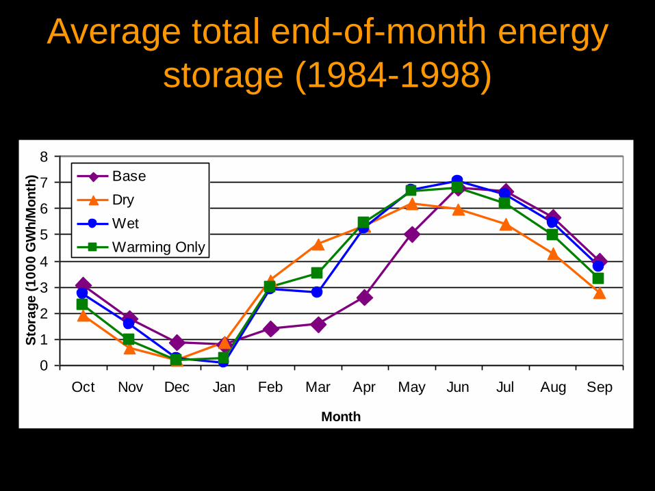
4.2. Reservoir Storage Changes with Climate Warming

Figure 6 shows how average end-of-month energy storage in all reservoirs combined

changes with climate when reservoirs are operated for energy revenues only. Under the

Base scenario, reservoirs reach their minimum storage level by the end of January to

prepare to capture expected inflow from winter precipitation and later spring snowmelt.

On average, reservoirs are full by June and gradually emptied for energy generation over

the summer when energy prices are higher and there is little natural inflow. Under

historical conditions, refill starts in January and drawdown starts in June. Although


12

climate warming results do not appear to change these cycles much, snowpack loss

generally increases average reservoir storage (stored energy) between February and May

than in the Base case. With dry climate warming, energy storage peaks earlier and

drawdown begins a month earlier.

4.3. Energy Spills with Climate Warming

Figure 7 shows the frequency of total monthly energy spill from the system for the study

period when the system is optimized for revenue maximization. Energy spill results from

runoff that can be neither stored nor sent through turbines because of limited capacities.

Energy spill is the equivalent energy value of the available runoff water which cannot

contribute to energy production at each site. Energy is spilled by the system in 30

percent of months under all climate scenarios, including the Base scenario. However, the

magnitude of spills increases for Wet and Warming-Only scenarios, and decreases for the

Dry scenario. Existing storage capacity cannot compensate for the loss of snowpack

during wetter years, and overall earlier snow melt, but appears able to compensate in

drier years.

What is calculated as energy spill in this study is the increased historic energy spill,

because annual historical generation (actual recorded output of the system) in each year

during 1984 to 1994 period was used as the annual energy input to calibrate the

hydropower system model, for which spill data are unavailable. However, the calculated

energy spill under the historic scenario is only 0.002 percent of total generation.


13

Figure 8 shows the distribution of total average monthly energy spill under different

climate scenarios. Under the historic climate scenario, energy spills occur from

December to June when inflow to the system peaks. The changes in the magnitude and

timing of spills under different climate warming scenarios indicate the importance of

runoff inflow timing and magnitude to the performance of this system.

Figure 9 plots the frequency curve of total annual spill from the system for the study

period. Energy does not spill under the Base scenario for most years. Annual energy

spill frequency and magnitude both increase with Wet and Warming-Only scenarios and

decrease with Dry warming. As more precipitation falls as rain than snow and snow

melts sooner at high elevation under climate warming, annual energy spills increase in

both size and frequency as monthly runoff distribution patterns and annual volumes no

longer match well with existing storage and generation capacities. Most energy spill

occurs under the Wet scenario, in more than 80 percent of years. Under the Warming-

Only and Dry scenarios, energy spills in more than 70 and 50 percent of years,

respectively.

4.4. Revenue and Energy Price Patterns under Climate Warming

Figure 10 indicates the climate warming effects on monthly average price for generated

energy. Climate warming generally increases average energy prices in more than 60

percent of months. As expected, the rise in prices is highest with dry climate warming


14

(given the non-linear relationship between electricity price and generation quantity).

Under this scenario prices are higher than the base case more than 90 percent of the time.

Average received energy price frequency curves for Wet and Warming-Only scenarios

show similar behavior, highlighting the importance of runoff timing over quantity for

optimal system operations.

Figure 11 shows the effects of climate warming on the frequency of total annual revenues

of all 137 hydropower plants studied for the period 1984 to 1998. Although monthly

average prices received for generated energy were higher under the Dry scenario, the

increase in prices does not compensate for the Dry scenario reduction in total energy

generation. Annual revenue under the Wet scenario exceeds Base scenario revenue in 60

percent of years but is almost the same during the rest of the time. Annual revenue under

the Warming-Only scenario is similar to the Base scenario.

In this study, the effects of climate warming on energy demand were neglected. To

improve the estimations, in future, the effects of climate change on energy demand can be

studied by defining different relationships between energy generation quantity and energy

price for various scenarios (Madani and Lund, submitted).

4.5. Benefits of expanding energy storage and generation capacity

Figure 12 shows, on average, how energy storage capacity expansion changes

hydropower generation revenues under different climate scenarios over the study period


15

(15 years). This figure indicates the average shadow price of energy storage capacity (the

increase in annual revenue per 1 MWh energy storage capacity expansion) for all 137

reservoirs. For instance, increase in annual revenue per 1 MWh energy storage capacity

expansion is less than $5 for 103 of the studied power plants under the Dry scenario.

Storage capacity expansion reduces spills and allows for more release in summer when

energy prices are higher. Storage capacity expansion can increase average annual

revenues for almost all hydropower plants under all climate scenarios, but such expansion

might not be justified due to expansion costs. As expected, benefits of capacity expansion

are greater for Wet and Warming-Only scenarios. The annual marginal benefit of storage

capacity expansion is greatest under the Wet scenario when more energy is available to

store. Even with the historical hydrology, expanding storage capacity increases total

annual revenues in all years because more storage capacity allows for more flexible

operations needed to generate more energy during peak price times. While about 100

hydropower plants benefit more from energy storage capacity expansion under the Base

scenario than the Dry scenario, the other 37 hydropower plants benefit more from energy

storage capacity expansion under the Dry scenario than the Base scenario.

Figure 13 indicates the average shadow price of energy generation capacity (the increase

in annual revenue per 1 MWh of monthly energy generation capacity expansion) for all

137 plants under different climate scenarios. Generation capacity expansion does not

increase the annual revenues of about 90 hydropower plants under the Base and Dry

scenarios. About 50 of the studied hydropower plants do not need energy generation

capacity expansion under all types of climate warming, meaning that those units do not


16

experience energy spill at all even with warmer climates. Although generation capacity

expansion produces benefits, expansion costs might be prohibitive. Similar to storage

capacity expansion, benefits of energy generation capacity expansion are higher under

Wet and Warming-Only than Base and Dry scenarios. Comparison of Figures 12 and 13

shows that energy storage capacity expansion is typically more beneficial than energy

generation capacity expansion if the expansion costs are the same.

5. Limitations

Models are not perfect and optimized results are optimized to particular conditions and

objectives. During model development many simplifying assumptions are made which

should be considered in interpreting the results. However, simulation and optimization

models are useful in studying resource management problems. Here, the results give

some insights on how the system works and how it might adapt under different climate

warming scenarios.

Calibration of EBHOM for this study (Madani and Lund, submitted) is likely to under-

estimate energy storage capacities and therefore also underestimate adaptability of the

system to climate change. Availability of spill or energy storage capacity data would

reduce this source of error.

California is big and variable in hydrology. Assuming the same seasonal pattern for

inflows in north and south at the same elevation will cause some inaccuracies. A 1000


17

feet range covers a great variability in hydrology. Smaller elevation ranges might

increase the accuracy of the estimation. Since many power plants are in the 3000-4000

feet elevation range, it might be worthwhile to study this range separately. Also, more

gauges might be considered for each elevation range.

As a first step in studying the adaptability of California’s high-elevation hydropower

system to climate warming, this study looks at flexibility of operations without

considering environmental constraints.

Here, energy prices were imposed on each individual power plant. Instead, total demands

might be imposed to the system of one hundred thirty-seven plants. This gives more

flexibility in operation and reaction of the system. High-elevation plants at lower

elevations which receive the peak flows earlier can generate more in earlier months while

higher plants generate more, later during the year. Although the timing of flow will

change, there is still a difference in flow patterns at different elevation ranges which

benefits the system if operated wisely. By integrating operations of individual

hydropower systems that span different watersheds and elevation bands, greater

operational flexibility to respond to changes in climate, streamflow, and runoff may be

possible.

With climate warming, demands are likely to increase in warmer months from higher

temperatures. This could affect energy prices. EBHOM employed recorded real-time

energy prices for finding revenue curves which define the relation between monthly


18

energy generation and energy price. The prices used here are from 2005 which do not

exactly match energy prices of the 1984 to 1995. This might cause some inaccuracies in

EBHOM’s estimation of revenues and energy prices. However, this limitation might not

affect the other results (generation, spill, and storage) much as the energy price trends are

similar over the years of study. Application of price data sets which are longer than one

year in future might improve the accuracy of model results.

For this application we assume inflow distributions adhere to a fixed seasonal pattern.

Inflow distributions are likely to be more local and vary more between years. Here, the

model optimizes revenue based on its perfect information about the year’s hydrological

pattern. Such management is impossible in practice.

6. Conclusions

In absence of detailed information about the available energy storage capacity at high-

elevation in California, this study applied a simple low-resolution approach for estimating

the adaptability of California’s high-elevation hydropower generation to climate

warming. Substituting the estimated energy content of runoff water inflows and storage

for these relatively high-head hydropower units and estimating seasonal inflow

distribution patterns by elevation band allowed preliminary optimization-driven monthly

system operations modeling of more than 137 hydropower plants with various climate

changes.


19

With climate warming, California loses snowpack which has functioned historically as a

natural reservoir to delay runoff, but considerable energy storage and generation capacity

remaining available. The EBHOM’s results show that most extra runoff in winter months

from climate warming can be accommodated by the available storage capacity at high-

elevation sites for average years. Lower-elevation reservoirs, constructed primarily for

water supply, already have substantial re-regulation capacity for seasonal flow

adjustments (Tanaka et al. 2006). However, operating rules should change with climate

warming to adapt the system to changes in hydrology (Medellin et al. 2008).

Generally, climate warming alone reduces high-elevation hydropower generation and

revenue, without changes in total runoff, due solely to changes in seasonal runoff timing.

Energy spills increase dramatically under Wet and Warming-Only scenarios with existing

storage and generation capacities. More storage capacity would increase revenues but

might not be cost effective. Storing water in reservoirs helps shift energy runoff

reductions to months with lower energy prices to reduce economic losses. More

generation capacity also increases revenues by reducing energy spill. Annual marginal

benefits of capacity expansion are higher for storage than for generation. Nevertheless,

current storage and generation capacities give the system some flexibility to adapt to

climate changr. Although the Dry scenario examined in this study has 20 percent less

runoff than the base historical hydrology, system-wide, revenues decrease by less than 12

percent through optimally re-operating storage and generation facilities within existing

capacity limits. Thus, the current storage and generation capacities can compensate for


20

some snowpack loss, and for the Wet and Warming-Only scenarios with very little

revenue decrease.

Limited capacities cannot take full advantage of increased energy runoff under the Wet

scenario. The Wet warming scenario examined here has 10 percent more runoff than the

historical hydrology, but only 5 percent more generation and 2 percent more average

annual revenues. In a Warming-Only scenario with unchanged historical precipitation,

generation and revenues decrease by 1.4 and almost 1 percent, respectively.

This study required some simplifying assumptions. Nevertheless, it gives insights and

suggests some degree of adaptive capability to climate warming. Future studies should

address environmental and other constraints, include demand and price impacts of

climate change, and apply refined estimates of varied hydrologic changes from climate

change across California.

Acknowledgments

The authors thank Omid Rouhani from University of California, Davis for his help in

EBHOM development, Marcelo Olivares from University of California, Davis for

providing hourly energy price data, Maury Roos from California Department of Water

Recourses for providing the names of reliable high-elevation gauges in California, and

Jery Stedinger from Cornell University for his early feed-back on the work. This work


21

was funded by the California Energy Commission’s Public Interest Energy Research

(PIER) program and the Resources Legacy Fund Foundation.

References

Aguado, E., D. Cayan, L. Riddle, M. Roos (1992); “Climate Fluctuations and the Timing

of West Coast Streamflow”; Journal of Climate, Vol. 5, pp. 1468-1483.

Aspen Environmental Group and M. Cubed (2005); “Potential changes in hydropower

production from global climate change in California and the western United States”;

California Climate Change Center, CEC-700-2005-010, June 2005

(http://www.energy.ca.gov/2005publications/CEC-700-2005-010/CEC-700-2005-

010.PDF).

Brekke, L.D., N.L. Miller, K.E. Bashford, N.W.T. Quinn, and J.A. Dracup, 2004.

“Climate Change Impacts Uncertainty for Water Resources in the San Joaquin River

Basin, California.” Journal of the American Water Resources Association, Vol. 40,

No. 1, pp. 149-164.

California ISO OASIS (2007), Hourly Average Energy Prices, California Independent

System Operator (ISO) Open Access Same-Time Information System (OASIS) web

site, http://oasis.caiso.com/ (May 2007).

Carpenter, T.M. and Georgakakos, K.P. (2001); “Assessment of Folsom lake response to

historical and potential future climate scenarios: 1. Forecasting”; Journal of

Hydrology, Vol. 249, pp. 148-175.

http://www.energy.ca.gov/2005publications/CEC-700-2005-010/CEC-700-2005-010.PDF

http://www.energy.ca.gov/2005publications/CEC-700-2005-010/CEC-700-2005-010.PDF

http://oasis.caiso.com/


22

Cayan, D.R., L.G. Riddle, and E. Aguado (1993); “The Influence of Precipitation and

Temperature on Seasonal Streamflow in California”; Water Resources Research,

Volume 29(4), pp 1127-1140.

CDWR (California Department of Water Resources) (1998); “The California Water Plan

Update”; Bulletin 160-98, Volume 1, California Department of Water Resources,

Sacramento, California.

Dettinger, M. D. and Cayan D. R. (1995); “Large-Scale Atmospheric Forcing of Recent

Trends toward Early Snowmelt Runoff in California”; Journal of Climate, Vol. 8(3),

pp. 606–623.

Dettinger, M.D., Cayan D. R., Meyer M. K., and Jeton A. E. (2004); “Simulated

Hydrologic Responses to Climate Variations and Change in the Merced, Carson, and

American River Basins, Sierra Nevada, California, 1900-2099”; Climatic Change,

Volume 62, pp. 283- 317.

Gleick, P.H. and Chalecki E. L. (1999); “The Impact of Climatic Changes for Water

Resources of the Colorado and Sacramento-San Joaquin River Systems”; Journal of

the American Water Resources Association, Vol. 35(6), pp. 1429-1441.

Glieck, P.H. (2000); “The Report of the Water Sector Assessment Team of the National

Assessment of the Potential Consequences of Climate Variability and Change”;

Pacific Institute for Studies in Development, Environment, and Security, Oakland,

California.

Haston, L., Michaelsen J. (1997); “Spatial and Temporal Variability of Southern

California Precipitation over the Last 400 yr and Relationships to Atmospheric

Circulation Patterns”; Journal of Climate, Vol. 10(8), pp.1836 1852.


23

IPCC (Intergovernmental Panel on Climate Change) (2001); “Climate Change 2001: The

Scientific Basis”; Cambridge University Press, Cambridge, United Kingdom, 881 pp.

Lettenmaier, D. P., Gan, T. Y. (1990); “Hydrologic Sensitivity of the Sacramento-San

Joaquin River Basin, California, to Global Warming”; Water Resources Research;

Vol. 26, No. 1, pp. 69-86.

Lettenmaier, D. P. and Sheer D. P. (1991); “Climatic Sensitivity of California Water

Resources,” Journal of Water Resources Planning and Management; Vol. 117, No. 1,

Jan/Feb, pp. 108-125.

Lund, J. R., Zhu T., Jenkins M. W., Tanaka S., Pulido M., Taubert M., Ritzema R.,

Ferriera I. (2003); “Climate Warming & California’s Water Future”; Appendix VII,

California Energy Commission: Sacramento. pp. 1–251

(http://www.energy.ca.gov/reports/2003-10-31_500-03-058CF_A07.PDF).

Madani, K., J.R. Lund, (2007a) “Aggregated Modeling Alternatives for Modeling

California’s High-elevation Hydropower with Climate Change in the Absence of

Storage Capacity Data,” Hydrological Science and Technology, Vol. 23, No. 1-4, pp.

137-146.

Madani K., J. R, Lund (2007b) “High-Elevation Hydropower and Climate Warming in

California”, Proceeding of the 2007 World Environmental and Water Resources

Congress, Tampa, Florida, (Ed) Kabbes K. C., ASCE.

Madani K., Lund J. R. (submitted) " Modeling California's High-Elevation Hydropower

Systems in Energy Units", Water Resources Research.

Madani K., S. Vicuna, J. Lund, J. Dracup, and L. Dale (2008); “Different Approaches to

Study the Adaptability of High-Elevation Hydropower Systems to Climate Change:

http://www.energy.ca.gov/reports/2003-10-31_500-03-058CF_A07.PDF


24

The Case of SMUD’s Upper American River Project”, Proceeding of the 2008 World

Environmental and Water Resources Congress, Honolulu, Hawaii, (Ed) Babcock R.

W. and Walton R., ASCE.

Medellín-Azuara J., Harou J. J., Olivares M. A., Madani K., Lund J. R., Howitt R. E.,

Tanaka S. K., Jenkins M. W., Zhu T. (2008); “Adaptability and Adaptations of

California’s Water Supply System to Dry Climate Warming”; Climatic Change. 87

(Suppl 1):S75–S90.

Meko, D.M., M.D. Therrell, C.H. Baisan, and M.K. Hughes (2001); “Sacramento River

Flow Reconstructed to A.D. 869 From Tree Rings”; Journal of the American Water

Resources Association (JAWRA); Vol. 37(4); pp. 1029-1039.

Miller, N. L., Bashford, K. E., and Strem, E. (2003); “Potential Impacts of Climate

Change on California Hydrology”; Journal of the American Water Resources

Association, Vol. 39(4), pp. 771-784.

Pew Center on Global Climate Change (2006); (www.pewclimate.org/global-warming-

basics/).

Snyder, M.A., J.L.Bell, L.C. Sloan, P.B. Duffy, and B. Govindasamy (2002); “Climate

Responses to a Doubling of Atmospheric Carbon Dioxide for a Climatically

Vulnerable Region”; Geophysical Research Letters; Vol. 29(11),

10.1029/2001GL014431.

Stine, S. (1994); “Extreme and Persistent Drought in California and Patagonia During

Medieval Time”; Nature, Vol. 369, pp 546-549.

http://www.pewclimate.org/global-warming-basics/

http://www.pewclimate.org/global-warming-basics/


25

Tanaka S. T., Zhu T., Lund J. R., Howitt R. E., Jenkins M. W., Pulido M. A., Tauber M.,

Ritzema R. S. and Ferreira I. C. (2006); “Climate Warming and Water Management

Adaptation for California”; Climatic Change; Vol. 76, No. 3-4.

VanRheenen, N.T., A.W. Wood, R.N. Palmer, D.P. Lettenmaier (2004); “Potential

Implications of PCM Climate Change Scenarios for Sacramento–San Joaquin River

Basin Hydrology and Water Resources”; Climatic Change; Vol. 62(1-3), pp. 257-281.

Vicuña S., Leonardson R., Dracup J. A., Hanemann M., Dale L. (2005); “Climate Change

Impacts on High Elevation Hydropower Generation in California’s Sierra Nevada: A

Case Study in the Upper American River”; California Climate Change Center, CEC-

500-2005-199-SD, December 2005

(http://www.energy.ca.gov/2005publications/CEC-500-2005-199/CEC-500-2005-

199-SF.PDF).

Vicuna S., R. Leonardson, M. W. Hanemann, L. L. Dale, and J. A. Dracup (2008)

Climate change impacts on high elevation hydropower generation in California’s

Sierra Nevada: a case study in the Upper American River, Climatic Change, 28

(Supplement 1), 123-137.

Zhu T. (2004); “Climate Change and Water Resources Management: Adaptations for

Flood Control and Water Supply”; Ph.D. Dissertation, University of California,

Davis.

Zhu T., Jenkins M. W., and Lund J. R. (2005); “Estimated Impacts of Climate Warming

on California Water Availability Under Twelve Future Climate Scenarios.” Journal of

the American Water Resources Association (JAWRA); Vol. 41(5):pp. 1027-1038.

http://www.energy.ca.gov/2005publications/CEC-500-2005-199/CEC-500-2005-199-SF.PDF

http://www.energy.ca.gov/2005publications/CEC-500-2005-199/CEC-500-2005-199-SF.PDF


26

Table 1. EBHOM’s results (average of results over 1984-1988 period) for different

climate scenarios

Base Dry Wet Warming-

Only

Generation (1000 GWH/yr) 22.3 18.0 23.4 22.0

Generation Change with Respect to the Base Case (%) - 19.3 + 4.8 - 1.4

Spill (MWH/yr) 433 224 1,661 735

Spill Change with Respect to the Base Case (%) - 46.0 + 283.9 + 58.8

Revenue (Million $/yr) 1,449 1,271 1,483 1,435

Revenue Change with Respect to the Base Case (%) - 12.3 + 2.3 - 0.9

0

5

10

15

20

25

30

35

40


Month

Perc

en

t o

f A

nn

ual

Ru

no

ff (

%)

1000-2000 ft

2000-3000ft

+3000 ft

Figure 1. Monthly runoff distributions at different elevation ranges


27

0

5

10

15

20

25

30

35

40


Month

Ru

n P

erc

en

t (%

)

Base

Dry

Wet

Warming Olny

a) 1000-2000 ft

0

5

10

15

20

25

30

35

40


Month

Perc

en

t o

f A

nn

ual

Ru

no

ff (

%)

Base

Dry

Wet

Warming Olny

b) 2000-3000 ft

0

5

10

15

20

25

30

35

40


Month

Perc

en

t o

f A

nn

ual

Ru

no

ff (

%)

Base

Dry

Wet

Warming Olny

c) + 3000 ft

Figure 2- Monthly runoff distributions for different climate change scenarios and

elevation ranges


28

0

0.1

0.2

0.3

0 0.02 0.04 0.06 0.08 0.1 0.12 0.14 0.16 0.18

Monthly Energy Generation Capacity (1000 GWh)

Es

tim

ate

d A

nn

ua

l E

ne

rgy

Sto

rag

e

Ca

pa

cit

y (

10

00

GW

h)

Figure 3. Range of the estimated energy storage and generation capacities of the 137

studied high-elevation hydropower plants in California

0

0.5

1

1.5

2

2.5

3

3.5


Month

Ge

ne

rati

on

(1

00

0 G

WH

/Mo

nth

) Base

Dry

Wet

Warming Only

Figure 4. Average monthly generation (1984-1998) under different climate scenarios

0

1

2

3

4

0% 20% 40% 60% 80% 100%

Non-Exceedence Probability

Ge

ne

rati

on

(1

00

0 G

WH

/Mo

nth

)

Base

Dry

Wet

Warming Only

Figure 5. Frequency of optimized monthly generation (1984-1998) under various climate

scenarios (all months, all years, all units)


29

0

1

2

3

4

5

6

7

8


Month

Sto

rag

e (

10

00

GW

h/M

on

th) Base

Dry

Wet

Warming Only

Figure 6. Average total end-of-month energy storage (1984-1998) under different

climate scenarios

0.0

0.5

1.0

1.5

2.0

2.5

3.0

70% 75% 80% 85% 90% 95% 100%


Sp

ill (

10

00

GW

H/M

on

th)

Base

Dry

Wet

Warming Only

Figure 7. Frequency of total monthly energy spill (1984-1998) under different climate

scenarios (all months, all years, all units)

0.0

0.1

0.2

0.3

0.4

0.5

0.6

0.7

0.8

0.9

1.0


Month

En

erg

y S

pill (1

000G

WH

/Mo

nth

)

Base Scen

Dry Scen

Wet Scen

Warming Only

Figure 8. Average monthly total energy spill (1984-1998) under different climate

scenarios


30

0

1

2

3

4

5

0% 20% 40% 60% 80% 100%


Sp

ill (

10

00

GW

H/M

on

th)

Base

Dry

Wet

Warming-Only

Figure 9. Frequency of total annual energy spill (1984-1998) under different climate

scenarios (all years, all units)

40

60

80

100

120

0% 20% 40% 60% 80% 100%


Ma

rgin

al E

ne

rgy

Pri

ce

($

/MW

H)

Base

Dry

Wet

Warming Only

Figure 10. Frequency of monthly energy price (1984-1998) under different climate

warming scenarios (all months, all years, all units)

0

400

800

1,200

1,600

2,000

0% 20% 40% 60% 80% 100%


An

nu

al R

ev

en

ue

(M

illio

n $

/yr)

Base

Dry

Wet

Warming-Only

Figure 11. Frequency of total annual revenue (1984-1998) under different climate

scenarios (all years, all units)


31

0

10

20

30

40

50

0 20 40 60 80 100 120

Number of Plants

$/Y

ea

r/M

Wh

Base

Dry

Wet

Warming-Only

Figure 12. Average shadow price of energy storage capacity of 137 hydropower units in

California in the 1984-1998 period under different climate scenarios

0

10

20

30

40

50

0 20 40 60 80 100 120

Number of Plants

$/Y

ear/

MW

h

Base

Dry

Wet

Warming-Only

Figure 13. Average shadow price of energy generation capacity of 137 hydropower units

in California in the 1984-1998 period under different climate scenarios

1

Modeling California’s High-Elevation Hydropower Systems in Energy Units 1

2

Kaveh Madani1 and Jay R. Lund

2 3

Department of Civil and Environmental Engineering 4

University of California, Davis, CA 95616, USA 5

Phone: 530-752-5671 Fax: 530-752-7872 6

Email: [email protected] /

[email protected] 7

Abstract 8

This paper presents a novel approach for modeling of high-elevation hydropower systems. 9

Conservation of energy and energy flows (rather than water volume or mass flows) are used as 10

the basis for modeling more than 130 high-elevation high-head hydropower sites throughout 11

California. The unusual energy basis for reservoir modeling allows for development of 12

hydropower operations models for a large number of plants to estimate large-scale system 13

behavior without the expense and time needed to develop traditional streamflow and reservoir 14

volume-based models in absence of storage capacity, penstock head, and efficacy information. 15

Potential applications of the developed Energy-Based Hydropower Optimization Model 16

(EBHOM) include examination of the effects of climate change and energy prices on system-17

wide generation and hydropower revenues. 18

19

Keywords: hydropower, high-elevation, electricity, optimization, reservoir operation, climate 20

change, California. 21

22

23



2

1. Introduction 24

Hydroelectric power’s low cost, near-zero pollution emissions, and ability to quickly respond to 25

peak loads make it a valuable renewable energy source. In the mid-1990s, hydropower was 26

about 19 percent of world’s total electricity generation (Lehner et al., 2005). Worldwide 27

hydroelectric generation from 1990 to 2020 could grow at an annual rate between 2.3 to 3.6 28

percent (European Commission, 2000; Lehner et al., 2005). 29

30

Depending on hydrologic conditions, hydropower provides 5 to 10 percent of the electricity used 31

in the United States (National Energy Education Development Project, 2007) and almost 75 32

percent of the nation’s electricity from all renewable sources (EIA, 2005; Wilbanks et al., 2007). 33

No electricity generation source is cheaper than hydropower. While it costs almost 4 cents and 2 34

cents to generate one kilowatt-hour (kWh) of electricity at coal plants and nuclear plants, 35

respectively, hydropower generation typically costs only about 1 cent per kWh (National Energy 36

Education Development Project, 2007). 37

38

About 75,000 megawatts of hydropower generation capacity exist in the U.S., equivalent 39

capacity to 70 large nuclear power plants (National Energy Education Development Project, 40

2007). More than half of U.S. hydroelectric capacity is in the western states of Washington, 41

California and Oregon, with approximately 27 percent in Washington (EIA, 2007). 42

Hydropower facilities in the U.S. are diverse. Facilities range from multi-purpose dams with 43

large reservoirs to small run-of-river dams with little or no active water storage (National Energy 44

Education Development Project, 2007). Plant elevations also vary. In California multi-purpose 45

3

dams are usually at lower elevations than plants served by reservoirs operating primarily for 46

hydropower. 47

48

California relies on hydropower for 9 to 30 percent of the electricity used in the state, depending 49

on hydrologic conditions (Aspen Environmental Group and M. Cubed 2005). California’s high-50

elevation hydropower system is composed of more than 150 power plants, above 305 meters 51

(1,000 feet) elevation. This system, which mostly relies on snowpack, supplies roughly 74 52

percent of California’s in-state hydropower, although only about 30 percent of in-state usable 53

reservoir capacity is at high elevations, above 305 meters (Aspen Environmental Group and M. 54

Cubed 2005). The high-elevation reservoirs are predominantly single-purpose reservoirs for 55

generating hydropower (Aspen Environmental and M-Cubed, 2005, Vicuna et al., 2008) whith 56

some secondary benefits such as flood control. These reservoirs which are mostly privately-57

owned are regulated by U.S. Federal Energy Regulatory Commission (FERC) and operated for 58

hydropower revenues only. The high-elevation hydropower plants are generally located below 59

small (within-year storage) reservoirs with high turbine heads compared with much larger multi-60

purpose reservoirs with low-turbine head downstream (lower elevations). 61

62

California’s Mediterranean climate has one wet season and a long dry season. On average, 75 63

percent of the annual precipitation occurs between November and March. These single-purpose 64

reservoirs (except for few such as Lake Almanor) are always emptied by the end of the 65

hydrologic year (September) to capture fall and winter precipitation and spring snowmelt. Since 66

electricity prices are high in summer, it is reasonable to generate and sell hydropower instead of 67

risking energy spill in the wet season when energy prices are lower. Therefore, only one major 68

4

drawdown-refill cycle per year typically occurs for hydropower and water supply operations in 69

California. 70

71

Hydropower generation varies greatly from year to year with varying inflows, as well as 72

competing water uses, such as flood control, water supply, recreation, and in-stream flow 73

requirements (for water rights, navigation, and protection of fish and wildlife) (National Energy 74

Education Development Project, 2007). Given hydropower’s economic value and its role in 75

complex water systems, it is reasonable to seek optimal operation of hydropower generation and 76

adaptation to changing conditions. Optimization models are common for studying the 77

performance of hydropower systems under different conditions and for deriving reservoir 78

operating policies. Conventional simulation and optimization methods used for hydropower 79

systems (Grygier and Stedinger, 1985; Arnold et al, 1994; Vicuna et al., 2008) are quite useful 80

but their application to extensive hydropower systems is intensive and costly. For instance, there 81

are 2,388 hydropower plants in the U.S., of which 411 plants are located in California (Hall and 82

Reeves, 2006). Studying climate change effects on hydropower generation in the U.S. or even in 83

California through conventional detailed modeling of each system requires large investments of 84

time and money, especially when basic information such as stream flows, turbine capacities, 85

storage operating capacities, and energy storage capacity are not readily available for each plant. 86

Given the proprietary nature of most existing hydropower models and data, there is value for a 87

less-detailed method of modeling extensive hydropower systems lacking detailed information. 88

The objective of this paper is to introduce a new method for studying optimal operation of high-89

elevation systems, which operate predominantly for hydropower, with high head and negligible 90

over-year storage, in absence of detailed information about the system, 91

5

92

Energy-based modeling of single-purpose hydropower systems is presented, along with 93

application to 137 hydropower plants throughout California. We begin with the general model 94

formulation, followed by novel methods for estimating the energy storage capacity of 95

hydropower units and representing hourly-varying prices in reservoir models at larger time 96

scales. A small change in the formulation is introduced for cyclic seasonal operations. 97

Comparison of model generation estimates is made with the historic generation in an average 98

hydrologic year at a particular facility in California (Loon Lake). Discussion of the general 99

estimation of parameters for 156 hydropower plants in California is made. Then the model is 100

applied to estimate optimal monthly energy generation at 137 hydropower plants in California 101

for a 15 year period. The paper concludes with a discussion of potential applications, limitations, 102

and conclusions. The primary advantage of this approach is to develop policy and operational 103

insights for large numbers of hydropower plants where traditional reservoir model development 104

and estimation would be prohibitively costly and time consuming. 105

106

2. Energy-Based Hydropower Optimization Model (EBHOM) 107

Unlike conventional models, where calculations are in volumetric units, the Energy-Based 108

Hydropower Optimization Model (EBHOM), introduced here, is a monthly-step model which 109

does all storage, release, and flow calculations in energy units. EBHOM is developed to 110

investigate the performance of the system under different conditions and can contribute to 111

studies in which the active storage capacity data and penstock head information are unavailable. 112

In such studies, energy storage capacity for each unit can be calculated based on differences in 113

6

seasonal water inflow distribution and energy generation data. EBHOM can then be applied to 114

explore the optimal operation of the system for different scenarios. 115

116

Most high-elevation hydropower plants operate for net revenue maximization (Jacobs et al., 117

1995). Lower elevation plants tend to operate for a greater variety of purposes. Since 118

hydropower operating costs are essentially fixed (at monthly scale), an operational surrogate for 119

net revenue maximization is revenue maximization. EBHOM’s simple general mathematical 120

formulation (in energy units) is: 121

Maximize

12

1

i i

i

Z P G (1) 122

Subject to: 123

S1 = 0 (initial condition) (2) 124

Si ≤ Scap (storage capacity), i (3) 125

Si = ei-1+Si-1- Ri-1 (conservation of energy), i (4) 126

Gi ≤ Ri, i (5) 127

Gi ≤ Gcap (generation capacity constraint), i (6) 128

Gi , Si , Ri ≥ 0 (non-negativity), i (7) 129

(i = 1, 2, 3, ... , 12) 130

131

where Z = revenue; Gi = hydropower generation in month i (MWh/month); Pi = price of 132

electricity in month i ($/MWh); Si = energy storage at the beginning of month i (MWh); Scap = 133

energy storage capacity (MWh); ei = energy runoff in month i (MWh); Ri = energy release from 134

the reservoir in month i (MWh/month) (decision variable); Gcap = generation capacity 135

7

(MWh/month); and i =1 corresponds to the first month of the refill cycle with energy storage at 136

the beginning of this month set equal to zero (Equation 2). 137

138

This formulation is valid when the reservoir is used only for hydropower generation, and 139

primarily for seasonal (as opposed to over-year) storage. The formulation also requires a “high-140

head” condition where storage does not significantly affect hydropower head. 141

142

3. Estimating Seasonal Energy Storage Capacity 143

Normal estimation of a reservoir’s energy storage capacity involves integrating the potential 144

energy content over all reservoir elevations, presuming detailed knowledge of penstocks, 145

reservoir geometries, and bank storage. Obtaining storage capacity data and penstock head 146

information for many individual reservoirs is a big obstacle in large-scale hydropower systems 147

modeling, especially if they belong to private owners with proprietary interests in information. 148

Even if volumetric storage capacities were available, conventional estimation of energy storage 149

capacities (that portion of the capacity storing water for electricity generation) would have been 150

tedious and probably unreliable. To estimate the energy storage capacity of each power plant, it 151

is assumed that the existing storage and release capacities of a high-elevation hydropower 152

reservoir are sufficient to operationally accommodate the historical runoff in an average water 153

year without water spilling from the reservoir. 154

155

The proposed No Spill Method (NSM) estimates seasonal energy storage capacity under the 156

following conditions: 157

8

1. The reservoir does not spill energy in the average year, and all releases are made through 158

the turbines. Energy spill results from runoff lost from the system because it can be neither 159

stored nor sent through the turbines due to limited storage and turbine capacities. Energy 160

spill is the equivalent energy value of the available runoff which cannot contribute to 161

energy production at a site. For California, this lack of spill in an average year was 162

confirmed in conversations with the private hydropower operators of most high-elevation 163

plants in California. This condition sets a lower bound for storage capacity estimation. 164

Actual reservoir capacity will exceed this lower bound if the reservoir does not fill in an 165

average year. However, for calculation purposes it is assumed that the reservoir fills in an 166

average year. This makes the approach pessimistic. 167

2. The power plant is a high-head facility, where the effect of reservoir storage level on 168

turbine head is small. Generally, turbine head in high-elevation hydropower facilities is 169

mostly from large penstock drops, rather than additional elevation within the reservoir. 170

This allows a linear relationship between the amount of water stored in the reservoir and 171

energy stored, and seems common for many proprietary models for this system. 172

3. The seasonal distribution of inflow is known. Average seasonal flow distributions from 173

nearby gages are used here to reflect seasonal runoff and snowmelt conditions. 174

4. There is only one major drawdown-refill cycle per year. Hydropower reservoirs typically 175

fill once each year in California. 176

High-elevation hydropower facilities usually have a within-year storage pool and mostly have 177

watersheds above 305 meters 1,000 feet. In California, many of these systems rely on snowpack 178

to increase the seasonal storage of the system. 179

9

180

The NSM estimates seasonal storage capacity in energy units by finding the area between the 181

monthly runoff and monthly generation curves when both are expressed as monthly percentages 182

of the annual average quantity. In month i, the runoff percentage (runoffPercenti) and generation 183

percentage (genPercenti) can be calculated by dividing the average monthly runoff in month i 184

(average runoffi) and the average monthly generation in month i (average generationi) to the 185

average annual runoff (average annual runoff) and the average annual generation (average 186

annual runoff), respectively. 187

ii

average runoffrunoffPercent

average annual runoff (8) 188

( )( )

average generation igenPercent i

average annual generation (9) 189

In percentage terms, the sum of differences between the two curves for a year (12 months) 190

should be zero. 191

12

1

( ) 0i i

i

runoffPercent genPercent (10) 192

In the 12 month period there are months i when the runoff percentage exceeds the generation 193

percentage value (when some runoff is stored in the reservoir) and months j when the generation 194

percentage exceeds the runoff percentage (when some hydropower is generated by releasing 195

stored water). 196

( ) ( ) 0i i j j

i j

runoffPercent genPercent genPercent runoffPercent (11) 197

So, if there is only one refill-drawdown cycle per year, little over-year storage, and the reservoir 198

is on the verge of spilling at its fullest, the seasonal storage capacity (StorCapPercent) as a 199

percent of total inflow is (Figure 1): 200

10

( )i i

i

StorCapPercent runPercent genPercent (12) 201

or: 202

( )j j

j

StorCapPercent genPercent runoffPercent (13) 203

Multiplying the storage capacity percentage (StorCapPercent) by the average annual generation 204

gives the active (operational) energy storage capacity (Scap). 205

Scap StorCapPercent average annual generation (14) 206

Multiplying the storage capacity percentage by the average annual runoff gives the volumetric 207

active (operational) water storage capacity (WScap) which is directly used for hydropower 208

generation. 209

WScap StorCapPercent average annual runoff (15) 210

Significantly, this method produces a lower bound estimate of energy storage capacity, as many 211

reservoirs will not spill or fill in wetter than average years. The NSM also assumes reservoirs 212

have negligible over-year storage, which is true for high-elevation hydropower reservoirs in 213

California with a few exceptions (such as Lake Almanor in California). 214

215

Figure 1 shows how the active storage capacity of the Buck Island (also known as Rubicon or 216

Loon Lake) Reservoir, with the storage capacity of 96 million cubic meters (mcm) (or 78 217

Thousand Acre-Feet (TAF)), located above Loon Lake Hydropower Plant with generation 218

capacity of 38 GWh per month and Average Annual Generation of 104 GWh in California was 219

estimated using NSM. Monthly generation data was available for the years 1984 to 1998. 220

Monthly runoff (inflow) data was obtained for the same period from U.S. Geological Survey 221

(USGS) gauges. The mean monthly and mean annual runoffs were estimated for the study 222

11

period. Mean monthly runoff and mean monthly generation values were then normalized into 223

percent of mean annual runoff (Equation 8) and mean annual generation (Equation 9), 224

respectively, as shown in Figure 1. Based on Equation 12 or 13, the shaded area between the 225

two curves (29 percent) represents the storage capacity as a percentage of total generation or 226

flow (StorCapPercent). Active storage capacity of this reservoir (the portion of actual energy 227

storage capacity used for storing water for hydropower) was found to be 31 GWh based on 228

Equation 14 and 13.6 mcm (11 TAF) based on Equation 15. 229

230

At a monthly time scale, several stair-stepped power houses (in series) might benefit from water 231

storage in one upstream reservoir. When one powerplant draws water from several upstream 232

reservoirs (in parallel or series) the energy storage calculated for the powerplant will reflect the 233

total effective energy storage upstream of the plant. For instance for 2 reservoirs in series, the 234

effective storage capacity belonging to the power station located below the second (lower) 235

reservoir is determined based on the difference between the undisturbed (natural) runoff to the 236

first reservoir and the energy outflow from the second powerplant. In that case, the calculated 237

storage capacity is equal to the effective storage capacity of the lower reservoir plus the portion 238

effective storage capacity of the upper reservoir used for regulating the inflow to the lower 239

reservoir. Indeed, in this case the difference between the runoff and generation curves could be 240

smaller if there was no up-stream reservoir. However, when an upstream reservoir exists, energy 241

is stored in the upper reservoir for some period, so the total effective storage capacity is higher 242

than the effective storage capacity of the lower reservoir. This can become a more complicated 243

issue, as inflows for downstream powerplants might be dominated by releases from upstream 244

plants, not the assumed monthly inflow distribution for the powerplant. Ultimately, this is one of 245

12

the limitations of such coarse less-detailed modeling. Incorporating such effects would require 246

much greater modeling effort, which we needed to avoid here. 247

248

4. Energy Price Representation 249

If fixed monthly energy prices are used in Equation 1, EBHOM is linear as done in studies by 250

Vicuna et al. (2008), and Madani and Lund (2007). However, if fixed monthly energy prices are 251

used, while maximizing revenue, the model suggests no generation in months with low energy 252

prices to allow more generation in months with higher average prices, within storage capacity 253

limits (Madani and Lund, 2007). In real electricity markets, prices fluctuate hourly and marginal 254

revenues of generation decrease with increased hours of generation. Linear EBHOM (monthly 255

basis model) does not capture the varying nature of energy prices and the considerable effects of 256

on-peak and off-peak pricing on the revenues. Considering on-peak and off-peak monthly prices 257

in the linear model (Vicuna et al., 2008) captures some effects of non-constant energy prices. It 258

is possible to capture the varying nature of energy prices by linear EBHOM if it is formulated on 259

an hourly basis. However, such a model takes much more time as it requires 730 times more 260

decision variables (with 730 hours in average month). To decrease calculation time and effort, 261

EBHOM can be formulated on a monthly basis as a concave non-linear problem to represent on-262

peak and off-peak price variability, with a revised objective function (Equation 1) as follows: 263

Maximize

12

1

( )i i i

i

Z P h G (16) 264

where average monthly energy price P(hi) is a function of total hours of generation in month i. 265

The variation in price with generation is not a result of price effects from an individual power 266

plant’s generation. Instead, this price variation represents the hourly variability in energy prices 267

of the overall energy market responding mostly to on-peak and off-peak variability in energy 268

13

demands. Price for an individual plant’s operation varies with the number of hours it operates. 269

Since these plants are run to maximize power revenues, they are assumed to be operated in hours 270

when the energy market offers higher prices. 271

272

If a plant operation is solely for hydropower, then the frequency distribution of hourly 273

hydropower prices (Figure 2) can be integrated into an average revenue function of turbine 274

release as a percent of monthly turbine capacity (Figure 3). If operating only for hydropower, a 275

utility will release first at high-valued times and only release at lower-valued times as water 276

becomes more abundant. The resulting benefit function allows approximate representation of 277

hourly pricing within a monthly model. Hourly price frequencies from 2005 are used to develop 278

revenue functions for each month (the 2005 prices were used only because of unavailability of 279

price data for earlier years). Figure 2 shows the frequency of real-time market hourly energy 280

prices in October 2005 in California, spanning on-peak and off-peak prices. For optimal 281

hydropower operations, average energy price declines as hours of generation increase, so small 282

releases are targeted for the maximum energy price and lowest average price occurs when release 283

equals generation capacity. Since monthly generation increases by increasing the hours of 284

turbine-run, it is assumed that the revenue from each hydropower plant is a function of the 285

portion of used monthly generation capacity: 286

( ) ( )i i i iz h z g (18) 287

where: gi is the portion of monthly generation capacity used. 288

ii

Gg

Gcap (19) 289

Integration over the price curve in a given month (Figure 2) gives that month’s revenue (zi) as 290

follows: 291

14

0

( ) . ( )ig

i i i i iz g Gcap P g dg (20) 292

293

Using Equation 20, concave revenue curves for each month (October in this example) can be 294

derived, as shown in Figure 3. In this figure, the horizontal axis shows gi (October), and the 295

vertical axis shows the corresponding average revenue per unit of plant generation capacity 296

(( )i iz g

Gcap). From Figure 3, if the power plant generates at its full capacity in October, revenue at 297

that power plant is 48 $/MWh times its generation capacity. Revenue curves for any given 298

fixed-head Californian hydropower plant in each month can be derived by multiplying both axes 299

of Figure 3 by generation capacity of that power plant. Such curves can then be piece-wise 300

linearized or included non-linearly, and summed over the months for the objective function of 301

EBHOM (Equation 16 as follows): 302

Maximize

12

1

( )i i

i

Z z g (21) 303

This formulation reflects the on-peak on off-peak pricing. The prices occur for the same hours of 304

the day, across all plants. The price does not decrease because of the quantity of energy 305

generated, but because of the hours of the day generated. 306

307

5. Reformulation for Cyclical Operations 308

The EBHOM, as defined earlier, can be sensitive to the initial storage condition (Equation 2). 309

Each reservoir has a specific refill and drawdown cycle. To find the best initial condition (refill 310

month) for a single reservoir, the EBHOM should be run 12 times for the 12 different possible 311

refill months, saving the decision values from the best performing refill month. 312

15

313

Although simple and comprehensible, running the model 12 times for each reservoir requires 314

excessive computation time for large systems. To decrease the calculation time the formulation is 315

revised by replacing the first two constraints (Equations 2 and 3) with the following four 316

constraints: 317

S1 =big (initial condition) (22) 318

Smin ≤ Si , i (23) 319

Si ≤ Smax, i (24) 320

Smax,- Smin ≤ Scap (storage capacity constraint) (25) 321

322

where big = an arbitrary large number greater than or equal to Scap; Smin = minimum monthly 323

energy storage during the year (12 months period) (a decision variable); and Smax = maximum 324

monthly energy storage during the year (a decision variable). 325

326

This formulation sets initial storage equal to a large nominal level (big). Storage changes are 327

then made conventionally around this nominal level, with storage constrained to return to this 328

initial level. The storage capacity constraint is enforced by defining the minimum and maximum 329

storages from all months (Equations 23 and 24), and then constraining the difference (Equation 330

25), which is the amplitude of the annual drawdown-refill cycle. This limits real storage within 331

the real storage capacity. Since the nominal initial storage exceeds the reservoir’s capacity, 332

nominal storage cannot be negative in any month. 333

334

335

16

6. Comparison for Loon Lake Power Plant 336

Figure 4 compares the average historic (recorded) hydropower generation (period 1982-2002) 337

and the EBHOM’s estimation of optimal monthly hydropower generation in an average 338

hydrologic year of the same period at Loon Lake Hydropower Plant, which belongs to the 339

Sacramento Municipal Utility District (SMUD) reservoir system. Assuming a fixed energy head, 340

un-regulated water runoff is linearly related to available energy runoff. Based on the No-Spill 341

assumption, total annual energy generation for a given hydropower plant (from observed energy 342

generation data) in a given year equals the annual available energy runoff at its location in that 343

year, and only the seasonal distributions differ. Accordingly, monthly distribution of energy 344

runoff in each year of the study period was assumed to be exactly the same as the distribution of 345

mean monthly runoff for the period 1928 to 1949. Monthly energy runoff was computed (for use 346

in Equation 4) based on the monthly runoff distribution given by the hydrologic record where 347

annual energy runoff equals the annual hydropower generation. Monthly revenue curves were 348

based on information from California Independent System Operator Open Access Same-Time 349

Information System Web Site for the year 2005 (California ISO OASIS, 2007). The non-linear 350

optimization problem was solved by linear programming through piecewise linearization of the 351

concave revenue function. 352

353

Generally, the difference of historic and modeled values is due to the mismatching runoff, 354

hydropower generation, and price data sets used, and non-energy hydropower operations such as 355

maintaining spinning reserves. The summer generation peak found by the model (in September) 356

is due to the high price of energy in September in the data set, which might not be true for the 357

period 1982 to 2002. Often hydropower generators pre-sell their power through long-term 358

17

contracts with fixed prices and control only that portion of hydropower generation not already 359

sold. A more extensive comparison of the EBHOM with a traditional hydropower optimization 360

model of the Sacramento Municipal Utility District (SMUD) reservoir system produced similar 361

results and showed good reliability of EBHOM predictions (Madani et al., 2008). 362

363

8. Estimation for 137 Plants in California 364

EBHOM was applied for modeling the high-elevation hydropower system in California. One 365

hundred fifty-six (156) high-elevation (above 305 meters or 1,000 feet) hydropower plants in 366

California were identified. Monthly hydropower energy generation information from U.S. 367

Energy Information Administration Databases for the period 1982 to 2002 was used to estimate 368

the average monthly hydropower energy generation and the generation capacity of each power 369

plant. Instead of using the name-plant capacity of each hydropower plant in this study, the 370

maximum actual monthly generation over the 1982-2002 period was used as the monthly 371

generation capacity. For estimating energy storage capacity available for each hydropower unit, 372

mean monthly generation and mean annual generation were estimated. Mean monthly values 373

were then normalized into percent of mean annual generation (Equation 9) to characterize the 374

average seasonal distribution of energy generation at each unit. Since runoff patterns vary by 375

elevation, three elevation ranges are considered (305-710 meters or 1,000-2000 feet, 710-915 376

meters or 2000-3000 feet, and above 915 meters or 3000 feet). Monthly runoff data for the study 377

period were obtained for several USGS gauges representing these elevation ranges, selected in 378

consultation with the former California Department of Water Resources (DWR) chief 379

hydrologist. For each elevation range, mean monthly and mean annual runoffs were estimated. 380

Mean monthly values were then normalized into percent of mean annual runoff (Equation 8) to 381

18

characterize the average seasonal distribution of available water runoff for each elevation range. 382

Energy storage capacity of each unit was then estimated using the NSM. Real time hourly 383

hydroelectricity prices were obtained from the California ISO OASIS for the year 2005 384

(California ISO OASIS, 2007) and used to derive convex monthly revenue curves. 385

386

EBHOM was used to estimate the optimal historic monthly generation. The EBHOM for each 387

plant was solved in Microsoft Excel (through piecewise linearization) with “What’sBest”, a 388

commercial solver package for Microsoft Excel. With the cyclic EBHOM formulation, each run 389

for one reservoir for each year under a given hydrology takes 3 to 4 seconds. Historical 390

generation data was complete for 137 high-elevation plants for the period of 1984-1998. The 391

piecewise-linear optimization model was run for each year to find revenue-maximizing monthly 392

reservoir storage and energy generation for these 137 power plants. The model was run with the 393

historical hydrology. Assuming no over-year storage, release decisions in each year are 394

independent. Figure 5 shows the range of the estimated energy storage and generation capacities 395

of the studied high-elevation hydropower plants. The annual energy storage capacities of most of 396

the studied power plants are at least 1.3 times larger than their monthly generation capacity, 397

which provides some flexibility in operations. For most power plants, energy storage capacity 398

exceeds one month of generation capacity. 399

400

Figure 6 shows the historical and modeled average energy generation of 137 hydropower plants 401

for the period 1984 to 1998. (The analysis has not been done for an average year but for 15 years 402

of hydrologic (energy inflow) annual variability, spanning dry, wet, and average years. The 403

19

results are reported as average over the 15 year period for which 15 model runs were required). 404

The optimized generation for the historic climate differs from historic observations (the dashed 405

curve in Figure 6). Differences arise from a variety of factors, including non-hydropower 406

operating factors, differences in hydropower prices from the recorded years, non-energy 407

hydropower operations such as spinning reserves, and the foresight of the model regarding 408

incoming flows during the year. Another reason for divergence between the EBHOM’s results 409

and the observed generation is application of a representative annual hydrograph for each 410

elevation band rather than locally measured inflows for each year. The generation results are 411

highly price driven and follow the California ISO energy price trends in 2005. 412

413

Figure 7 shows the average end-of-month energy storage in all reservoirs combined in the study 414

period for operations optimized for hydropower. EBHOM suggests that reservoirs reach their 415

minimum storage level by the end of January in preparation to capture inflow from winter 416

precipitation and spring snowmelt. On average, reservoirs are full by June and gradually empty 417

for energy generation over summer when energy prices are higher and there is little natural 418

inflow. Under historical conditions, refill starts in February and drawdown starts in July. 419

420

Figure 8 indicates the average shadow prices of energy storage and generation capacities (the 421

average increase in annual revenue per unit of capacity expansion) for all 137 reservoirs for the 422

study period. This figure shows the average increase in annual revenue (y-axis) per MWh 423

energy storage/generation capacity expansion for corresponding number of power plants (x-424

axis). For instance, increase in annual revenue is less than $10 revenue per MWh energy storage 425

20

capacity expansion for 50 of the studied power plants. Generally, storage capacity expansion is 426

more beneficial than generation capacity expansion. Water can be stored in the reservoir in low-427

value months to be released in summer when energy prices are higher. Thus, shadow price of 428

energy storage capacity always exceeds the shadow price of generation capacity for all the 429

reservoirs. Generation capacity expansion does not increase average revenue of about 90 430

hydropower plants while energy storage capacity expansion always increases annual revenues. 431

Although expansion of storage and generation capacities can increase average annual revenues, 432

expansions might not be justified due to expansion costs. In some cases, where hydropower 433

plants are in series and draw on the same upstream reservoir, the value of expanding that 434

reservoir would be the sum of storage expansion values for all downstream plants. Since the 435

NSM (No-Spill Method) tends to underestimate energy storage capacities, the values for storage 436

capacity expansion are probably high estimates. 437

438

9. EBHOM Applications 439

Generally, an EBHOM can be applied in any hydropower system operation study where there is 440

relatively little effect of storage on head and there is an interest in the big picture of the system 441

and details are of lesser importance (e.g. large-scale policy, preliminary planning, and adaptation 442

studies). Some potential applications are discussed below. 443

444

Climate warming is a hydropower concern in regions with significant snowmelt runoff, such as 445

California. High-elevation hydropower systems in California rely on snowpack for seasonal 446

storage of precipitation, which makes those systems more vulnerable to climate warming 447

(Vicuna et al., 2008; Madani and Lund, 2007). EBHOM is convenient for studying climate 448

21

change effects on large-scale hydropower systems. Monthly runoff (energy inflow) can be 449

perturbed for various climate change scenarios. The effects of several climate scenarios can be 450

calculated quickly to allow quick, broad system-scale studies to accompany narrower 451

conventional hydropower optimization studies (Vicuna et al., 2008). 452

453

Effects of energy demand/pricing changes on hydropower generation and resulting downstream 454

flows also can be studied using EBHOM. Greater energy demand increases energy prices. 455

Currently, electricity is more expensive in summer and winter months from cooling and heating. 456

Energy demand can change for various climatic, economic, technologic, policy, or market 457

reasons. Climate warming also can reduce winter energy demand and prices (for heating) and 458

increase demand and prices in summer (for cooling). Energy prices also might change from 459

changes in supply. For instance, more energy generation in early spring from earlier snowmelt 460

might reduce energy prices in that period. Energy prices also can change with long-term changes 461

in energy-use technologies (e.g. for heating and cooling), economic growth, energy market 462

conditions (availability of non-hydropower energy supplies), energy conservation, or energy 463

regulatory policies. The effects of changes in energy prices on hydropower generation can be 464

studied conveniently by developing representative revenue curves (similar to Figure 3) for 465

conditions of interest. 466

467

In some parts of the world, large-scale expansions of hydropower storage and generation are 468

being contemplated. EBHOM formulations can be used to preliminary explore and identify 469

22

promising types and locations of power plant expansions, employing the Lagrange multiplier 470

(shadow price) results for energy storage and generation capacity constraints. 471

472

A final application of this type of coarse model might be for seasonal energy production and 473

market studies and forecasts. A coarse EBHOM can quickly give seasonal energy planners and 474

schedulers insights into when and how much hydropower is likely to be produced over a coarse 475

seasonal horizon, although operators are likely to have access to more detailed proprietary 476

models. 477

478

5. Limitations 479

The No-Spill Method (NSM) for estimating energy storage capacity should be applied to the 480

systems where there is little or no spill in many years and there is little over-year storage. 481

Nevertheless, the NSM will tend to under-estimate storage capacities and therefore also 482

underestimate the adaptability of the hydropower system to hydrologic and economic conditions. 483

More detailed studies could provide better estimates of energy storage capacities. 484

485

For this application to California, we assume that inflow distributions adhere to a fixed seasonal 486

pattern, which seem reasonable for California’s Mediterranean climate. This EBHOM is 487

formulated without considering environmental flows. Environmental constraints sometimes 488

restrict the flexibility of operations and introduce trade-offs between hydropower generation 489

revenues and ecosystem conservation benefits. These tend to be less for high-elevation 490

reservoirs, but will probably increase with time. Environmental constraints could be 491

23

incorporated in the model as minimum releases or as changes in the objective function or the 492

frequency distribution of prices. 493

494

EBHOM is a deterministic model and optimizes generation based on perfect foresight for 495

seasonal inflows and the frequency distribution of prices. Such management is impossible in 496

practice, because of imperfectability of forecasts of hydrologic and price conditions. Long-term 497

generation contracts also will affect operations. 498

499

6. Conclusions 500

This study introduced an innovative approach for exploring the performance of high-elevation 501

hydropower systems without detailed information on volumetric storage capacity, inflow, or 502

geometric configuration. Estimation of energy storage capacity is made based on seasonal shifts 503

of energy inflows to generation, energy inflows are based on seasonal inflow distributions, and 504

generation capacity is estimated from maximum observed generation rates. 505

506

The goal of this study was to explore an approach for studying extensive multi-facility high-head 507

hydropower systems with minimal available information and efficient. This approach is used to 508

represent 137 high-elevation (high-head) units in California. The method required some 509

simplifying assumptions. EBHOM can be applied in high-elevation hydropower operation 510

studies examining climate change effects and adaptations for hydropower generation, the effects 511

of electricity demand and pricing changes on hydropower generation, early planning for 512

extensive capacity expansions, and seasonal energy forecast and scheduling studies. 513

514

24

The contributions of this work are: 515

1. An energy-unit based model (Energy-Based Hydropower Optimization Model or 516

EBHOM) of single-purpose hydropower generation systems, requiring little model 517

development effort for low-detailed modeling. 518

2. The No-Spill Method (NSM) for estimating energy storage capacity. 519

3. A price-frequency method of better representing hourly energy prices in models with 520

larger time steps. 521

4. A cyclic storage formulation to decrease the calculation time and cost. 522

5. A simple approach for developing a good representation of an extensive system with little 523

time or resources for policy and adaptation studies for various purposes. 524

525

Acknowledgements 526

The authors thank Omid Rouhani from University of California, Davis for his help in EBHOM 527

development, Marcelo Olivares from University of California, Davis for hourly energy price 528

data, Sebastian Vicuna from University of California, Berkeley for the historical runoff data and 529

other information for the Loon Lake Hydropower Plant, Maury Roos from California 530

Department of Water Recourses for the names of reliable high-elevation gauges in California, 531

Jery Stedinger from Cornell University for his early feed-back on the work, and Rolf Larsson 532

from Lund University and the anonymous reviewers for their constructive comments. This work 533

was funded by the California Energy Commission’s Public Interest Energy Research (PIER) 534

program and the Resources Legacy Fund Foundation. 535

536

537

25

References 538

Arnold E., P. Tatjewski, and P. Wolochowicz (1994) Two methods for large-scale nonlinear 539

optimization and their comparison on a case study of hydropower optimization, J. of Optimiz. 540

Theory App, 81 (2), 221-248. 541

California ISO OASIS (2007) Hourly Average Energy Prices, California Independent System 542

Operator (ISO) Open Access Same-Time Information System (OASIS) web site, 543

http://oasis.caiso.com/ (May 2007). 544

EIA (2005) Renewable Energy Trends 2004, Table 18, Renewable Electric Power Sector Net 545

Generation by Energy Source and State, 2003, Energy Information Administration, 546

Washington, DC. 547

Energy Information Administration (2007) Energy Kid’s Page available at: 548

http://www.eia.doe.gov/kids/energyfacts/sources/renewable/water.html, November 6, 2007 549

European Commission (2000) 1999 annual energy review, Energy in Europe special issue—550

January 2000, Directorate-General for Energy, Brussels, ISBN 92-828-7448-6. 551

Grygier, J.C. and J.R. Stedinger (1985) Algorithms for Optimizing Hydropower System 552

Operation, Water Resour. Res., 21, 1-10. 553

Hall D. G. and K. Reeves (2006) A Study of United States Hydroelectric Plant Ownership, 554

Report prepared for the National Renewable Energy Laboratory, Idaho National Laboratory, 555

INL/EXT-06-11519. 556

Jacobs J., Freeman G., Grygier J., Morton D., Schultz G., Staschus K., and Stedinger J. (1995) 557

SOCRATES: A system for scheduling hydroelectric generation under uncertainty, Annals of 558

Operations Research, 59 (1), 99-133. 559

http://oasis.caiso.com/

http://www.eia.doe.gov/kids/energyfacts/sources/renewable/water.html

26

Lehner B., G. Czischb, and S. Vassolo (2005) The impact of global change on the hydropower 560

potential of Europe: a model-based analysis, Energ. Policy (33), 839–855. 561

Madani K. and J. R, Lund (2007) High-Elevation Hydropower and Climate Warming in 562

California, Proceeding of the 2007 World Environmental and Water Resources Congress, 563

Tampa, Florida, (Ed) Kabbes K. C., ASCE. 564

Madani K., S. Vicuna, J. Lund, J. Dracup, and L. Dale (2008) Different Approaches to Study the 565

Adaptability of High-Elevation Hydropower Systems to Climate Change: The Case of 566

SMUD’s Upper American River Project”, Proceeding of the 2008 World Environmental and 567

Water Resources Congress, Honolulu, Hawaii, (Ed) Babcock R. W. and Walton R., ASCE. 568

National Energy Education and Development Project (2007) Hydropower, Secondary Info Book, 569

pp. 24-27. 570

Vicuna S., R. Leonardson, M. W. Hanemann, L. L. Dale, and J. A. Dracup (2008) Climate 571

change impacts on high elevation hydropower generation in California’s Sierra Nevada: a 572

case study in the Upper American River, Climatic Change, 28 (Supplement 1), 123-137. 573

Wilbanks T. J., T. Bhatt, D. E. Bilello, S. R. Bull, J. Ekmann, W. C. Horak, Y. J. Huang, M. 574

D. Levine, M. J. Sale, D. K. Schmalzer, and M. J. Scott (2007) Effects of Climate Change on 575

Energy Production and Use in the United States, Synthesis and Assessment Product 4.5, 576

Report by the U.S. Climate Change Science Program and the Subcommittee on Global 577

Change Research, October 2007. 578

579

580

581

582

27

Figure Captions 583

Figure 1- Calculation of operational storage capacity of Loon Lake Reservoir based on NSM. 584

The shaded area between the two curves stands for the storage capacity of the reservoir in 585

percentage terms. 586

Figure 2. Frequency of California’s hourly hydroelectricity price in October 2005 (California 587

ISO OASIS, 2007) 588

Figure 3. Revenue-generation correlation in October 2005 (California ISO OASIS, 2007) 589

Figure 4- Comparison of average historic monthly electricity generation and optimal monthly 590

electricity generation (found by EBHOM) at Loon Lake Hydropower Plant in California 591

Figure 5. Comparison of historic average monthly electricity generation and optimal average 592

monthly electricity generation (found by EBHOM) of 137 hydropower units in California in 593

the 1984-1998 period 594


monthly electricity generation (found by EBHOM) of 137 hydropower units in California in 596

the 1984-1998 period 597

Figure 7. Average modeled total end-of-month energy storage (found by EBHOM) of 137 598

hydropower units in California in the 1984-1998 period 599

Figure 8. Average shadow prices of monthly energy generation and energy storage capacities 600

(found by EBHOM) of 137 hydropower units for California in the 1984-1998 period 601

602

603

604

605

28

606

Figure 1- Calculation of operational storage capacity of Loon Lake Reservoir based on NSM. 607

The shaded area between the two curves stands for the storage capacity of the reservoir in 608

percentage terms. 609

0

50

100

150

200

250

300

0% 20% 40% 60% 80% 100%

Exceedence Probability

Pri

ce (

$/M

WH

)

610

Figure 2. Frequency of California’s hourly hydroelectricity price in October 2005 (California 611

ISO OASIS, 2007) 612

runoffPercent

genPercent

StorCap

(%)

Pri

ce (

$/M

Wh

)

29

0

5

10

15

20

25

30

35

40

45

50

0% 20% 40% 60% 80% 100%

Monthly Genaration Capacity Used

Reven

ue/G

en

era

tio

n C

ap

acit

y (

$/M

WH

)

613

Figure 3. Revenue-generation correlation in October 2005 (California ISO OASIS, 2007). 614

Vertical axis shows the average revenue (in $) per unit of plant generation capacity (in MWh). 615

0

5

10

15

20


Month

Ge

ne

rati

on

(1

00

0M

Wh

)

Historic

Modeled

616

Figure 4 - Comparison of average historic monthly electricity generation and optimal monthly 617

electricity generation (found by EBHOM) at Loon Lake Hydropower Plant in California 618

Monthly Generation Capacity Used

Reven

ue/G

en

era

tio

n C

ap

acit

y (

$/M

Wh

)

30

0

0.1

0.2

0.3

0 0.02 0.04 0.06 0.08 0.1 0.12 0.14 0.16 0.18

Monthly Energy Generation Capacity (1000 GWh)

Es

tim

ate

d A

nn

ua

l E

ne

rgy

Sto

rag

e

Ca

pa

cit

y (

10

00

GW

h)

619

Figure 5. Range of the estimated energy storage and generation capacities of the 137 studied 620

high-elevation hydropower plants in California 621

0

1

2

3


Month

Ge

ne

rati

on

(1

00

0 G

WH

/Mo

nth

)

Historic

Modeled

622


monthly electricity generation (found by EBHOM) of 137 hydropower units in California in the 624

1984-1998 period 625

h)

31

0

1

2

3

4

5

6

7


Month

Sto

rag

e (

10

00

GW

h/M

on

th)

626

Figure 7. Average modeled total end-of-month energy storage (found by EBHOM) of 137 627

hydropower units in California in the 1984-1998 period 628

0

5

10

15

20

25

30

0 20 40 60 80 100 120

Number of Plants

$/Y

ea

r/M

Wh

Generation Capacity

Storage Capacity

629

Figure 8. Average shadow prices of monthly energy generation and energy storage capacities 630

(found by EBHOM) of 137 hydropower units for California in the 1984-1998 period 631

h)

Climate Change: Implications for Reservoir Management and Hydroelectricity in · PDF...

Documents

Transcript of Climate Change: Implications for Reservoir Management and Hydroelectricity in · PDF...