Classification images reveal decision variables andstrategies in forced choice tasksLisa M. Pritchett and Richard F. Murray1

Department of Psychology and Centre for Vision Research, York University, Toronto, ON, Canada M3J 1P3

Edited by Brian A. Wandell, Stanford University, Stanford, CA, and approved May 5, 2015 (received for review November 24, 2014)

Despite decades of research, there is still uncertainty about howpeople make simple decisions about perceptual stimuli. Mosttheories assume that perceptual decisions are based on decisionvariables, which are internal variables that encode task-relevantinformation. However, decision variables are usually considered tobe theoretical constructs that cannot be measured directly, and thisoften makes it difficult to test theories of perceptual decisionmaking. Here we show how to measure decision variables onindividual trials, and we use these measurements to test theories ofperceptual decision making more directly than has previously beenpossible. We measure classification images, which are estimates oftemplates that observers use to extract information from stimuli.We then calculate the dot product of these classification imageswith the stimuli to estimate observers’ decision variables. Finally,we reconstruct each observer’s “decision space,” a map that showsthe probability of the observer’s responses for all values of the de-cision variables. We use this method to examine decision strategiesin two-alternative forced choice (2AFC) tasks, for which there areseveral competing models. In one experiment, the resulting decisionspaces support the difference model, a classic theory of 2AFC de-cisions. In a second experiment, we find unexpected decision spacesthat are not predicted by standard models of 2AFC decisions, andthat suggest intrinsic uncertainty or soft thresholding. These exper-iments give new evidence regarding observers’ strategies in 2AFCtasks, and they show how measuring decision variables can answerlong-standing questions about perceptual decision making.

vision | psychophysics | classification images | signal detection theory |decision making

Many current questions about human cognition are relatedto how people make decisions, including decisions based

on perceptual information. For example, how do we decidewhether a search target is present in a cluttered display? How dowe decide when to respond in a task where both speed and ac-curacy are important? How do we judge which of two signals ispresent in a discrimination task?Most theories of perceptual decision making rely on the notion of

a decision variable, a quantity that the observer calculates from thestimulus to summarize task-relevant information, e.g., the proba-bility that a faint signal is present in a detection task (1). Sometheories of decision making are very simple, e.g., the observer givesone response if the decision variable is greater than a fixed criterion,and another response if the decision variable is less than the cri-terion. Other theories use more complex decision rules. Testingtheories of decision making would be much easier if we had accessto observers’ decision variables, but these are usually thought of astheoretical constructs that cannot be measured psychophysically.Here we show that in some tasks, it is possible to estimate decisionvariables on individual trials, and this provides a very direct way oftesting theories of perceptual decision making. We use this methodto examine the long-standing question of how people make de-cisions in two-alternative forced choice (2AFC) tasks.

Proxy Decision VariablesOur approach relies on the linear template model that has beenshown to account for performance in many simple discrimination

tasks (2, 3). In this model, the decision variable is the dot productof a template with the stimulus, plus a sample of normally dis-tributed internal noise. Previous work has shown that we canestimate an observer’s template by measuring a “classificationimage,” which is a map that shows the impact of small luminancefluctuations in each region of the stimulus on the observer’s re-sponses (4–6). A stimulus region that has a large effect on theobserver’s responses has a large value in the classification image,and a stimulus region that has little or no effect has a small value.Thus, a classification image shows what stimulus regions an ob-server uses to perform a task, and eliminates the need to make onetype of assumption about how the observer uses the stimulus.Motivated by the linear template model, we estimate ob-

servers’ decision variables by taking the dot product of theclassification image with the stimulus on each trial. We call theresult of this dot product a “proxy decision variable.” The proxydecision variable is an informative but imperfect estimate of thetrue decision variable, and we return to this point after discussingtheories of decision making in 2AFC tasks.

Decision Making in 2AFC TasksIn a 2AFC task, the observer views two signals in random orderand judges which order was shown (7). This task has played animportant role in perception research for over 60 years. It hasoften been used as a method of reducing observer bias, but moreimportantly, it has also been a testing ground for theories ofperceptual decision making.The classic model of 2AFC decisions is the “difference

model.” This model assumes that the observer calculates a de-cision variable from each of the two stimulus intervals and makesa response based on which decision variable is greater (7). Auseful tool for understanding such decision strategies is the de-cision space, a map that shows the probability of the observer’sresponses for all values of the decision variables (8). The dif-ference model implies that the observer’s decision space is di-vided into two response regions by a diagonal line (Fig. 1A): the

Significance

Signal detection theory is a classic theory of perceptual decisionmaking. This theory states that when people make a decisionbased on visual or auditory information, they calculate a “de-cision variable” that encodes their estimate of the probability ofeach possible response being correct. Until now, there has beenno way to measure decision variables behaviorally. We describea method of estimating decision variables, andwe show that it isa highly effective way of revealing peoples’ decision strategies.This creates a new approach to answering long-standing ques-tions about perception and decision making.

Author contributions: L.M.P. and R.F.M. designed research, performed research, analyzeddata, and wrote the paper.

The authors declare no conflict of interest.

This article is a PNAS Direct Submission.1To whom correspondence should be addressed. Email: rfm@yorku.ca.

This article contains supporting information online at www.pnas.org/lookup/suppl/doi:10.1073/pnas.1422169112/-/DCSupplemental.

www.pnas.org/cgi/doi/10.1073/pnas.1422169112 PNAS | June 9, 2015 | vol. 112 | no. 23 | 7321–7326

PSYC

HOLO

GICALAND

COGNITIVESC

IENCE

S

observer gives one response if the first decision variable isgreater, and the other response if the second decision variable isgreater, so the dividing line, or decision line, is y = x.Alternative models of 2AFC decisions have also been pro-

posed. According to the “double detection model,” the observermakes independent decisions about which signal was shown inthe first stimulus interval and which was shown in the secondinterval (9, 10). When the observer judges that both intervalscontain the same signal (which does not happen in a 2AFC task),the observer guesses. Under this model, the decision space isdivided into four quadrants (Fig. 1B). According to the “single-interval model,” the observer simply ignores one interval, andthe decision space is divided by a vertical or horizontal line (Fig.1C). In the “difference model with guessing,” the observercompares decision variables from the two stimulus intervals, as inthe difference model, but if the decision variables differ by lessthan a threshold amount, then the observer guesses (11). Herethe decision space is divided into three regions by two diagonallines (Fig. 1D).Previous studies have tested these models by comparing ob-

servers’ performance under various conditions in 2AFC tasksand other designs (9–11). However, different tasks put differentdemands on poorly understood factors such as attention andmemory, so these comparisons can be difficult to interpret (12).A recent review of studies on the 2AFC task concludes that weknow very little about how people actually make 2AFC decisions,and that the standard theory of 2AFC tasks, including the dif-ference rule, has little experimental support (10). Here we take anew approach to the problem of understanding peoples’ strate-gies in 2AFC tasks: We measure proxy decision variables in thetwo stimulus intervals over thousands of trials, and we use thesemeasurements to reconstruct observers’ decision spaces.

Proxy Decision SpaceThe proxy decision variable is the dot product of an observer’sclassification image with the stimulus. This gives an imperfectestimate of the true decision variable for at least two reasons:The classification image is an imperfect estimate of the template(3–6), and the observer has internal noise (1). In SI Text, Prop-erties of the Proxy Decision Space, we show that both these factorsimply that the proxy decision variable is equal to the true de-cision variable plus a normal random variable that representsmeasurement error. The “proxy decision space” is a map thatshows the probability of the observer’s responses for all values ofthe proxy decision variables. In SI Text, Properties of the Proxy

Decision Space, we also show that the measurement error in theproxy decision variables implies that the proxy decision spacedoes not have sharp edges, as in Fig. 1 A–D, but instead is thetrue, sharp-edged decision space convolved with a Gaussian kernelwhose scale constant is the standard deviation (SD) of the mea-surement error. For instance, an observer who uses the differencerule will produce a blurred proxy decision space, as in Fig. 1E, insteadof a sharp-edged space, as in Fig. 1A. For this reason, when fitting amodel to a proxy decision space, we require an SD parameter σblurthat controls the amount of blurring, in addition to parameters thatcontrol the position and orientation of the decision lines.

Experiment 1Task. In our first experiment, three observers discriminated be-tween black and white Gaussian profile disks in noise, at fixation,with two 500-ms stimulus intervals separated by a blank 1,000-msinterstimulus interval. Fig. S1 and Movie S1 show typical stimuli.Each observer ran in 9,900 trials. We calculated each observer’sclassification image and took its dot product with the two stim-ulus intervals on every trial. We constructed each observer’sproxy decision space by finding the probability of the observerresponding “black disk first” for all values of the two proxy de-cision variables. The data from both experiments reported in thispaper and MATLAB code implementing all our analyses areavailable at purl.org/NET/rfm/pnas2015.

Results. Fig. 2A shows the resulting proxy decision spaces, whichare divided diagonally, consistent with the difference model orthe difference model with guessing (Fig. 1 A and D). Modelselection via 10-fold cross validation supports this observation(Fig. 3). For all observers the cross-validation error was the samefor the difference model and the difference model with guessing,and significantly lower than for the double detection and single-interval models (P < 0.05 for within-observer, independentsamples t tests between the means of the difference model andthe double detection model, and between the means of the dif-ference model and the single-interval model, Bonferroni cor-rected for six comparisons). The difference model performs aswell as the difference model with guessing, but with one lessparameter, which supports the difference model as the bettermodel of performance on this task.As another test of the four models (Fig. 1 A–D), we fitted each

model to each observer’s decision space (Fig. 2A) and calculatedthe Akaike information criterion (AIC) of the fits (13). AICevaluates goodness of fit in a way that penalizes larger numbersof parameters. For all three observers, the difference model hadthe lowest AIC (see Table S1), showing again that it gave thebest account of observers’ data, consistent with our cross-vali-dation results.As a further test for a guessing region, we collapsed the de-

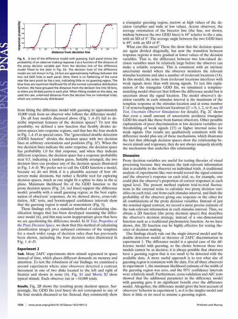
cision spaces parallel to the fitted decision line of the differencemodel, which is a line approximately halfway between the twored lines in each observer’s panel in Fig. 2A (to be discussedbelow). The difference model predicts that the transition be-tween response regions follows a normal cumulative distributionfunction, whereas the difference model with guessing predicts aflattening of the curve in the guessing region where the twodecision variables are approximately equal. Fig. 4 shows that thenormal cumulative distribution function (blue line) gives an ex-cellent fit, with no flattened interval apparent for any of theobservers. To find confidence intervals for the width of theguessing region, we bootstrapped fits of the difference modelwith guessing to the data shown in Fig. 4. For the panels from leftto right, the maximum likelihood estimates and 95% confidenceintervals for the width of the guessing region were 0.00 (0.00,0.29), 0.00 (0.00, 0.25), and 0.00 (0.00, 0.00). We conclude thatthere is little or no role for a guessing region in these observers’decision rules.

−1 −0.5 0 0.5 1−1

−0.5

0

0.5

1

resp

onse 2

resp

onse 1

−1 −0.5 0 0.5 1−1

−0.5

0

0.5

1

resp

onse 2

resp

onse 1

guess

guess

dec

isio

n v

aria

ble

2

decision variable 1

0

0.1

0.2

0.3

0.4

0.5

0.6

0.7

0.8

0.9

1

−1 −0.5 0 0.5 1−1

−0.5

0

0.5

1

resp

onse 2

resp

onse 1

−1 −0.5 0 0.5 1−1

−0.5

0

0.5

1

response 2

response 1guess

guess

−1 −0.5 0 0.5 1−1

−0.5

0

0.5

1

response 2

response 1

pro

bab

ility

−1 −0.5 0 0.5 1−1

−0.5

0

0.5

1

resp

onse 2

resp

onse 1gues

s

A B C

D E F

Fig. 1. Decision spaces for 2AFC decision models. Color encodes the proba-bility of the observer’s responses. (A) Difference model. (B) Double detectionmodel. (C) Single-interval model. (D) Difference model with guessing. (E) Proxydecision space for the difference model, with blur due to internal noise.(F) GDD function.

7322 | www.pnas.org/cgi/doi/10.1073/pnas.1422169112 Pritchett and Murray

In fact, even these relatively small bootstrapping estimatesoverstate the evidence for a guessing region in our data. Fig. S2(blue line) plots response probability as a function of the dis-tance from the center of the guessing region, according to thedifference model with guessing with a guessing region 0.30 unitswide (the upper limit of the bootstrapped 95% confidence in-tervals reported above) and an SD parameter σblur = 0.25 (atypical fitted value). With a guessing region this size, the re-sponse probability smoothly transitions from one side of thedecision line to the other, with no apparent flattening in themiddle. This occurs because, as we explained in the Introduction,the proxy decision space is a blurred version of the true decisionspace, and so a guessing region that is small relative to theamount of blur is effectively blurred out of the proxy decisionspace. Indeed, Fig. S2 (dashed green line) shows that the differencemodel with an SD parameter of σblur = 0.30 gives a psychometricfunction that is practically identical to the psychometric functionwith a guessing width of 0.30 (blue line), without the need for anadditional guessing width parameter.In Monte Carlo simulations, we generated artificial data from the

difference model, and we fitted the difference model with guessingto these data. We matched the parameters of the simulated differ-ence model and the number and distribution of trials to the psy-chometric function shown in Fig. 4, Left. These simulations assignedthe guessing region width a 95% confidence interval of (0.00, 0.30),simply due to the randomness in the simulated observer’s responses.This confidence interval is similar to those we found for two of threehuman observers, and the third observer’s confidence interval waseven smaller. (We include MATLAB code for this simulation in thecode posted at purl.org/NET/rfm/pnas2015.)In summary, our bootstrapping results show that Fig. 2A is

consistent with a guessing region up to 0.30 units wide, but our

cross-validation and AIC tests show that the difference modelgives a better account of the data, and our Monte Carlo simula-tions show that the 95% confidence intervals we found for humanobservers’ guessing regions are no larger than one would expect

Fig. 2. Proxy decision spaces. Each panel shows results from a single observer, based on ∼10,000 trials. The axes are the proxy decision variables for the twostimulus intervals, and the plots show the response probability as coded in the color bar. Red lines are maximum likelihood fits of the GDD function.(A) Probability of a “black disk first” response in the black/white discrimination task. (B) Probability of a “right disk brighter” response in the contrast in-crement detection task. (C) Probability of a “signal in interval 2” response from simulated model observers with intrinsic uncertainty. U is the number ofirrelevant mechanisms that the model observer monitors in each stimulus interval.

LMP MD MDC400

450

500

550

observer

neg

ativ

e lo

g li

kelih

oo

d

differencedifference with guessingdouble detectionsingle interval

Fig. 3. Results of 10-fold cross-validation. The y axis shows the negative loglikelihood of the observer’s responses on validation trials, averaged acrossthe 10 cross-validation blocks. Error bars show the SEM. The single-intervalbars show results averaged across a model that used only the first intervaland a model that used only the second interval; the results for these twosingle-interval models were practically identical.

Pritchett and Murray PNAS | June 9, 2015 | vol. 112 | no. 23 | 7323

PSYC

HOLO

GICALAND

COGNITIVESC

IENCE

S

from fitting the difference model with guessing to approximately10,000 trials from an observer who follows the difference model.Do all four models discussed above (Fig. 1 A–D) fail to de-

scribe important features of the decision spaces? To test thispossibility, we defined a new function that flexibly divides de-cision spaces into response regions, and that has the four modelsin Fig. 1 A–D as special cases. The “generalized double detection(GDD) function” divides the decision space with two decisionlines at arbitrary orientations and positions (Fig. 1F). When thetwo decision lines indicate the same response, the decision spacehas probability 1.0 for that response, and when they indicatedifferent responses, the decision space has a response probabilitynear 0.5, indicating a random guess. Suitably arranged, the twodecision lines can produce any of the decision spaces illustratedin Fig. 1 A–D. We prefer not to call the GDD function a model,because we do not think it is a plausible account of how ob-servers make decisions, but rather a flexible tool for exploringdecision spaces, much as one might fit a spline to data in the xyplane. Maximum likelihood fits of the GDD function to theproxy decision spaces (Fig. 2A, red lines) support the differencemodel, possibly with a small guessing region, as the best expla-nation of observers’ responses. As we showed above, cross-vali-dation, AIC tests, and bootstrapped confidence intervals showthat the guessing region is small or nonexistent (Fig. 3).These findings rely on a standard method of calculating clas-

sification images that has been developed assuming the differ-ence model (6), and this may seem inappropriate given that herewe are questioning the difference model. In SI Text, Properties ofthe Proxy Decision Space, we show that this method of calculatingclassification images gives unbiased estimates of the templatefor a much wider range of decision rules than has previouslybeen shown, including the four decision rules illustrated inFig. 1 A–D.

Experiment 2Task. Many 2AFC experiments show stimuli separated in spaceinstead of time, which places different demands on memory andattention. To test the robustness of our findings, we examined asecond experiment where nine observers detected a contrastincrement in one of two disks located to the left and right offixation and shown in noise (4). Fig. S1 and Movie S2 showtypical stimuli. Each observer ran in ∼10,000 trials.

Results. Fig. 2B shows the resulting proxy decision spaces. Sur-prisingly, the GDD fits (red lines) do not correspond to any ofthe four models discussed so far. Instead, they consistently show

a triangular guessing region, narrow at high values of the de-cision variables and wide at low values. Across observers, theaverage orientation of the bisector line (the line, not shown,midway between the two GDD lines) is 44° relative to the x axis,with an SD of 4°. The average angle between the two GDD linesis 49°, with an SD of 8°.What can this mean? These fits show that the decision spaces

are again divided diagonally, but now the transition betweenresponse regions is more gradual at lower values of the decisionvariables. That is, the difference between two low-valued de-cision variables must be relatively large before the observer canmake a reliable response. This is consistent with an intrinsicuncertainty model where the observer monitors the relevantstimulus locations and also a number of irrelevant locations (14).In this model, the noise from irrelevant locations interferes withweak signals more than with strong signals. To test this expla-nation of the triangular GDD fits, we simulated a template-matching model observer that follows the difference model but isuncertain about the signal location. The model observer’s de-cision variable in each stimulus interval is the maximum of thetemplate response at the stimulus location and at some numberU of nonoverlapping irrelevant locations (U = 0, 1, 2, or 8; see SIText, Uncertain Observer Simulations for details). Fig. 2C showsthat even a small amount of uncertainty produces triangularGDD fits much like those from human observers. Other possibleexplanations of poor discrimination at low decision variables arethresholding of weak signals (15) or higher internal noise forweak signals. Our results are qualitatively consistent with thedifference model plus any of these mechanisms, which illustratesthe fact that although decision spaces show the relationship be-tween stimuli and responses, they do not always uniquely identifythe mechanism that underlies this relationship.

DiscussionProxy decision variables are useful for testing theories of visualprocessing because they measure the task-relevant informationthat is available to the observer on individual trials. A traditionalanalysis of experiments like ours would record the signal contrastand the observer’s response on each trial, so, for example, onecould plot the observer’s proportion of correct responses at eachsignal level. The present method exploits trial-to-trial fluctua-tions in the external noise to calculate two proxy decision vari-ables on each trial, one from each stimulus interval, and finds theprobability of the observer giving one response or the other forall combinations of the proxy decision variables. Instead of justthe nominal signal contrast, we record a more precise estimate ofthe task-relevant information in each stimulus interval. Thus, weobtain a 2D function (the proxy decision space) that describesthe observer’s decision strategy, instead of a one-dimensionalfunction such as a traditional psychometric function. As we haveshown, this 2D function can be highly effective for testing the-ories of decision making.Our findings clearly rule out the single-interval model and the

double detection model as theories of 2AFC discrimination inexperiment 1. The difference model is a special case of the dif-ference model with guessing, so the choice between these twomodels cannot be as decisive; it is always possible that observershave a guessing region that is too small to be detected with theavailable data. A more useful approach is to test what size ofguessing region is consistent with the data. For all three observersin experiment 1, the maximum likelihood estimate of the width ofthe guessing region was zero, and the 95% confidence intervalswere relatively small. Furthermore, cross-validation and AIC testsshowed that the additional parameter in the difference modelwith guessing gave it no significant benefit over the differencemodel. Altogether, the difference model gives the best account ofobservers’ behavior in experiment 1, as it is the simpler model andthere is little or no need to assume a guessing region.

distance from decision line

resp

on

se p

rob

abili

ty

−1 −0.5 0 0.5 10

0.2

0.4

0.6

0.8

1

−1 −0.5 0 0.5 1 −1 −0.5 0 0.5 1

Fig. 4. A test of the difference model with guessing. Each panel shows theprobability of an observer making response 2 as a function of the distance ofthe proxy decision variable pair from the decision line of the differencemodel fitted to the data in Fig. 2A. The decision lines of the differencemodel are not shown in Fig. 2A but are approximately halfway between thetwo red GDD lines in each panel. Here, there is no flattening of the curvenear the zero point on the x axis, indicating little or no guessing region. Theblue lines are maximum likelihood fits of the normal cumulative distributionfunction. We have grouped the distances from the decision line into 50 bins,so there are 50 data points in each plot. When fitting models to this data, weused the raw, unbinned distances from the decision line on individual trials,which are continuously distributed.

7324 | www.pnas.org/cgi/doi/10.1073/pnas.1422169112 Pritchett and Murray

The proxy decision spaces we measured in experiment 2 didnot match the predictions of any of the four classic 2AFCmodels, and this is one of the most interesting findings of ourexperiments. The proxy decision spaces were roughly symmetricaround the 45° diagonal line, similar to the decision spaces of thedifference model and the difference model with guessing, whichsuggests that observers followed some variant of these models.Model observer simulations showed that a similar proxy decisionspace is produced by a difference model that is limited by afactor such as intrinsic uncertainty that worsens performance atlow signal levels. The difference model with guessing, limited byintrinsic uncertainty, would presumably produce a similar de-cision space. In experiment 2, it is difficult to choose between thedifference model and the difference model with guessing, be-cause uncertainty worsens performance in a triangular regionthat covers the diagonal region where the difference model withguessing predicts that a guessing region will appear (Fig. 1D).Furthermore, some care is necessary in interpreting experi-

ment 2, as intrinsic uncertainty does not fit neatly into ourmodeling tools. The linear observer model does not capturespatial uncertainty, because an uncertain observer monitorsmany signal detection mechanisms simultaneously, e.g., a spa-tially uncertain observer monitors many spatial locations for thesignal. This means that the observer effectively uses multipletemplates (one for each location), and one consequence of this isthat classification images give a blurred estimate of the ob-server’s template (16). Experiment 1 led to clear and easily in-terpretable findings. Experiment 2 is less decisive, but it showsthat the proxy decision variable method is open-ended and canreveal unexpected properties of observers’ decision strategies,much like the classification image method that it builds on.The literature on visual perception shows that in many tasks,

observers are unable to use an optimal strategy despite extensivepractice (e.g., refs. 14 and 17), and we should similarly expectthat observers’ decision spaces sometimes will be optimal andsometimes will not. The difference model is the optimal strategyin a 2AFC task with Gaussian noise (1). Experiment 1 gaveobservers an excellent chance to use or learn this optimal strat-egy: Observers ran in thousands of trials, in a simple foveal task,with auditory feedback on every trial. We found that in this ex-periment, observers did use the optimal strategy. However, ob-servers did not use the optimal strategy in experiment 2, whichwas different in seemingly minor ways: The stimuli were sepa-rated in space instead of time, they were just 0.5 degrees to theleft and right of the fovea, and observers judged which stimulushad a brightness increment instead of which was black or white.Thus, even small changes in a task can produce qualitative dif-ferences in behavior. There are currently no general rules forpredicting decision strategies, and they will need to be investi-gated case by case until generalizations become possible.Beyond testing models of 2AFC decisions, the proxy decision

variable method should be useful whenever it would be in-formative to have trial-by-trial estimates of observers’ decisionvariables. For example, most models of response times are basedon decision variables that fluctuate over time, accumulating in-formation until they reach a state that causes the observer tomake a response (18). If we show stimuli in dynamic noise, takethe dot product of the observer’s classification image with eachframe of noise, and sum these dot products over successiveframes, we may be able to estimate how an observer’s decisionvariable evolves over time on individual trials (compare the ap-proach in ref. 19). To take another example, one influentialtheory of visual search states that the observer calculates a de-cision variable from each target or distractor element in thesearch display and responds “target present” if the maximum ofthese decision variables exceeds a criterion (20). Proxy decisionvariables could give estimates of the decision variable from eachsearch element, and these measurements could be used to test

the maximum rule model of visual search. These examples il-lustrate how methods like the one we have presented can be usedto test theories that are based on decision variables. Decisionvariables have previously been thought of as inaccessible theo-retical constructs, but our experiments show that, in some cir-cumstances, they are measurable, and these measurements leaddirectly to new tests of sensory processing and decision making.

Materials and MethodsExperiment 1: Black/White Discrimination Task. Each observer ran in 33 blocksof 300 trials. Each trial showed two 500-ms stimulus intervals separated by ablank 1,000-ms interstimulus interval. Fig. S1 and Movie S1 show typicalstimuli. The signals were black and white Gaussian profile disks with scaleconstant σ = 0.055 degrees of visual angle (°). The black and white signalswere randomly assigned to the two stimulus intervals. The observer pressed akey to indicate the order of the signals, and received auditory feedback. Oneach trial, the white disk had peak luminance +L above the backgroundluminance of 65 cd/m2, and the black disk had peak luminance −L below thebackground luminance. The luminance perturbation L was adjusted acrosstrials according to a one-up two-down staircase converging on 71% correctperformance (21). The disks were shown in Gaussian white noise: The lumi-nance of each stimulus pixel was randomly perturbed by a value drawn froma normal distribution with mean zero and SD 16.25 cd/m2. A faint fixationpoint was shown continuously before and after the stimulus intervals. Tominimize spatial uncertainty, a thin white square surrounding the stimuluslocation was always present on the screen, and there was a small tick in themiddle of each side to indicate the center of the square. The stimuli were0.81° square (31 × 31 pixels). Viewing distance was 1.65 m. In each block,trials 101–150 were repeated as trials 151–200 (that is, the staircase wassuspended for trials 151–200, and these trials were exact repetitions of trials101–150), but we do not examine response consistency in this paper. Stimuliwere shown on a Sony Trinitron G520 monitor (512 × 384 resolution, pixelsize 0.755 mm, refresh rate 75 Hz). We show results for three observers. Afourth observer’s thresholds rose sharply over the course of the experiment,probably due to a loss of motivation; it is not meaningful to analyze all ofthis observer’s trials in a single decision space, so we discarded this data.

Experiment 2: Contrast Increment Detection Task. The data for this experimentare taken fromMurray et al.’s (4) experiment 2 (Fig. 2B, Top) and experiment3 (Fig. 2B, Middle and Bottom). Each observer ran in 50 blocks of 200 trials.Fig. S1 and Movie S2 show typical stimuli. The stimulus showed two disksof radius 0.11° positioned 0.50° to the left and right of a fixation point.The baseline luminance of the disks was 3 cd/m2 above the backgroundluminance of 30 cd/m2, and on each trial, one of the disks had a luminanceincrement. The luminance increment was set to each observer’s 70%threshold, based on pilot trials. Threshold luminance increments rangedfrom 1.2 cd/m2 to 2.1 cd/m2 across observers. The observer pressed a key toindicate which disk was brighter, and received auditory feedback. In Murrayet al.’s (4) experiments 2 and 3, observers gave rating responses on a six-pointscale, and we converted these to two-alternative responses by groupingratings 1–3 to mean “left disk brighter” and grouping ratings 4–6 to mean“right disk brighter.” The stimuli were shown in Gaussian white noise: Theluminance of each pixel of the stimulus was randomly perturbed by a valuedrawn from a normal distribution with mean zero and SD 6 cd/m2. The stimuliwere 1.0° vertical × 2.0° horizontal (38 × 76 pixels). The stimulus duration was200 ms. Viewing distance was 1.0 m. Stimuli were shown on an AppleVisionmonitor (640 × 480 resolution, pixel size 0.467 mm, refresh rate 67 Hz). Al-though the stimulus contrast was set to an estimate of each observer’s 70%threshold, performance ranged from 69% to 80% correct across observers.

Proxy Decision Spaces. We calculated each observer’s classification imageusing the weighted sum method for 2AFC tasks (6). To reduce measurementnoise, we radially averaged each classification image around the center ofthe signal (6) and set the classification image to zero at locations far fromthe center. To calculate proxy decision variables p1 and p2 for the twostimulus intervals, we took the dot product of the observer’s classificationimage with the two stimuli on each trial.

We constructed three 20 × 20 matrices, K = ðkijÞ, N= ðnijÞ, and P = ðpijÞ, torepresent the proxy decision space, as follows. We chose 20 evenly spacedvalues, x1, ..., x20, that spanned the range of the proxy decision variables inincrements of Δx. Each element nij was set to the total number of trials forwhich xi −Δx=2≤p1 < xi +Δx=2 and xj −Δx=2≤p2 < xj +Δx=2. Each elementkij was set to the number of trials in this range where the observer gaveresponse 2 (“black disk first” in experiment 1, “right disk brighter” in

Pritchett and Murray PNAS | June 9, 2015 | vol. 112 | no. 23 | 7325

PSYC

HOLO

GICALAND

COGNITIVESC

IENCE

S

experiment 2). Each pij was set to kij=nij. In Fig. 2, we show the matrix Protated 90° counterclockwise.

We used the same trials to calculate classification images and proxy de-cision spaces, but there is little danger of overfitting the classification images:We used ∼10,000 trials to estimate each small, radially pooled classificationimage, which had effectively just six or seven free parameters. In any case,we show in SI Text, Properties of the Proxy Decision Space, that any mea-surement error in the classification images simply increases the blur in theproxy decision spaces.

Modeling. The GDD function has five parameters: θ1 and δ1 that control theorientation and position, respectively, of the first decision line; θ2 and δ2 thatcontrol the second decision line; and γ that controls the probability of re-sponse 2 in the guessing regions. According to the GDD function, theprobability of response 2 when the decision variables are d1 and d2 is

DGDDðd1,d2; θ1, θ2, δ1, δ2, γÞ= PðR= 2jd1,d2Þ [1]

DGDDðd1,d2; θ1, θ2, δ1, δ2, γÞ

=

8><>:

1

0

γ

if  ðd1,d2Þ•ðcosðθ1Þ, sinðθ1ÞÞ≥ δ1   and  ðd1,d2Þ•ðcosðθ2Þ, sinðθ2ÞÞ≥ δ2

if  ðd1,d2Þ•ðcosðθ1Þ, sinðθ1ÞÞ< δ1   and  ðd1,d2Þ•ðcosðθ2Þ, sinðθ2ÞÞ< δ2

otherwise

.

[2]

Here, • is the vector dot product. The other models we considered are specialcases of this function. The difference model is

DDðd1,d2; δÞ=DGDDðd1,d2; 3π=4,3π=4, δ, δ, 0Þ. [3]

The double detection model is

DDDðd1,d2; δ1, δ2, γÞ=DGDDðd1,d2; π, π=2, δ1, δ2, γÞ. [4]

The single-interval model for the first interval is

DS1ðd1,d2; δÞ=DGDDðd1,d2; π, π, δ, δ, 0Þ. (5)

The single-interval model for the second interval is

DS2ðd1,d2; δÞ=DGDDðd1,d2; π=2, π=2, δ, δ, 0Þ. (6)

The difference model with guessing is

DDMGðd1,d2; δ1, δ2, γÞ=DGDDðd1,d2; 3π=4,3π=4, δ1, δ2, γÞ. (7)

In Eqs. 3, 5, and 6, we set γ =0 because there are no guessing regions inthese models.

We fit thesemodels to the proxy decision spacematrices K andN describedin Proxy Decision Spaces as follows. We will use the double detection modelDDD for illustration. This model has three parameters: δ1, δ2, and γ. Observers’responses had only small biases, so we fixed the guessing parameter toγ = 0.5. As we show in SI Text, Properties of the Proxy Decision Space, theproxy decision space is the true decision space convolved with a Gaussian

kernel, so we added another parameter σ to account for this blurring effect.Thus, we optimized parameters Θ= ðδ1, δ2, σÞ. For a given choice of param-eters, we first calculated a 20 × 20 matrix MðΘÞ= ðmijÞ representing thepredicted decision space, setting mij =DDDðxi , xj ; δ1, δ2, γÞ where xi and xj arethe values used to construct the proxy decision space matrices as described inProxy Decision Spaces. Next, we blurred MðΘÞ by a Gaussian kernel GðσÞwithscale constant σ to obtain a 20 × 20 matrix representing the predicted proxydecision space, QðΘÞ= ðqijÞ=MðΘÞ *GðσÞ, where * is 2D convolution. To avoidedge effects, we extendedMðΘÞ by 3σ on each side. To make the model fittingmore robust against occasional keypress errors or lapses in attention, we madethe probabilities in the proxy decision space saturate at 0.01 and 0.99, by de-fining ~QðΘÞ= ð~qijÞ= ðmaxðminðqij , 0.99Þ, 0.01ÞÞ. We used MATLAB’s fminsearchfunction to find the parameter values that minimized the negative loglikelihood of the observed proxy decision space matrices N and K,

Θ̂=argminΘ

−Xij

log�b�kij ,nij , ~qijðΘÞ

��. [8]

Here, bðk,n,pÞ is the binomial probability mass function. To make the fittingroutines more reliable, we took the best fit of 20 fits with randomly chosenstarting points. In Fig. S3, we show the results of 20 independent fits of theGDD function to each observer’s proxy decision space, to show that thefitting algorithm reliably converged to the global minimum.

The data from both experiments and MATLAB code that implements allour analyses are available online at purl.org/NET/rfm/pnas2015.

Cross-Validation. For cross-validation, we randomly divided each observer’strials into 10 equally sized blocks. On each cross-validation run, we used nineblocks for training and one block for validation. We measured the observer’sclassification image, decision variables, and proxy decision space on thetraining blocks, using the methods described in Proxy Decision Spaces. Tofind the cross-validation error for a given model (e.g., the difference model),we fitted the model to the proxy decision space from the training trials,using the methods described in Modeling. We then used the fitted model tofind the negative log likelihood of the observer’s responses in the valida-tion block. We did this by taking the dot product of the classificationimage (measured from the training blocks) with the two stimulus intervalsof each validation trial, producing two proxy decision variables ðp1,p2Þ. Wethen calculated the probability p of the observer making response 2 giventhe proxy decision variables ðp1,p2Þ, according to the fitted model beingtested. If we let r = 1 on trials where the observer gave response 2 and r = 0where the observer gave response 1, then the negative log likelihood ofthe observer’s response is −logðrp+ ð1− rÞð1−pÞÞ. The negative log likeli-hood of all responses in the validation block is the sum of this negative loglikelihood over all validation trials.

ACKNOWLEDGMENTS. We thank Minjung Kim, Yaniv Morgenstern, theeditor, and two anonymous reviewers for comments on the manuscript, andJames Elder and Laurie Wilcox for helpful discussions. This work was fundedby grants to R.F.M. from the Natural Sciences and Engineering ResearchCouncil and the Canada Foundation for Innovation.

1. Green DM, Swets JA (1966/1974) Signal Detection Theory and Psychophysics (Kreiger,Malabar, FL).

2. Murray RF, Bennett PJ, Sekuler AB (2005) Classification images predict absolute effi-ciency. J Vis 5(2):139–149.

3. Murray RF (2011) Classification images: A review. J Vis 11(5):2.4. Murray RF, Bennett PJ, Sekuler AB (2002) Optimal methods for calculating classifi-

cation images: Weighted sums. J Vis 2(1):79–104.5. Ahumada AJ, Jr (2002) Classification image weights and internal noise level estima-

tion. J Vis 2(1):121–131.6. Abbey CK, Eckstein MP (2002) Classification image analysis: Estimation and statistical

inference for two-alternative forced-choice experiments. J Vis 2(1):66–78.7. Tanner WP, Jr, Swets JA (1954) A decision-making theory of visual detection. Psychol

Rev 61(6):401–409.8. Ashby FG, Gott RE (1988) Decision rules in the perception and categorization of

multidimensional stimuli. J Exp Psychol Learn Mem Cogn 14(1):33–53.9. Treisman M, Leshowitz B (1969) The effects of duration, area, and background in-

tensity on the visual intensity difference threshold given by the forced-choice pro-cedure: Derivations from a statistical decision model for sensory discrimination.Percept Psychophys 6(5):281–296.

10. Yeshurun Y, Carrasco M, Maloney LT (2008) Bias and sensitivity in two-interval forcedchoice procedures: Tests of the difference model. Vision Res 48(17):1837–1851.

11. García-Pérez MA, Alcalá-Quintana R (2010) The difference model with guessing ex-plains interval bias in two-alternative forced-choice detection procedures. J Sens Stud25(6):876–898.

12. Wickelgren WA (1968) Unidimensional strength theory and component anal-

ysis of noise in absolute and comparative judgments. J Math Psychol 5(1):

102–122.13. Akaike H (1974) A new look at statistical model identification. IEEE Trans Automat

Contr 19(6):716–723.14. Pelli DG (1985) Uncertainty explains many aspects of visual contrast detection and

discrimination. J Opt Soc Am A 2(9):1508–1532.15. Pelli DG, Farell B, Moore DC (2003) The remarkable inefficiency of word recognition.

Nature 423(6941):752–756.16. Tjan BS, Nandy AS (2006) Classification images with uncertainty. J Vis 6(4):

387–413.17. Gold JM, Murray RF, Bennett PJ, Sekuler AB (2000) Deriving behavioural receptive

fields for visually completed contours. Curr Biol 10(11):663–666.18. Ratcliff R, Smith PL (2004) A comparison of sequential sampling models for two-

choice reaction time. Psychol Rev 111(2):333–367.19. Wilder JD, Aitkin C (2014) Saccadic timing is determined by both accumulated evi-

dence and the passage of timeJ Vis 14(10), 753 (abstr).20. Palmer J, Verghese P, Pavel M (2000) The psychophysics of visual search. Vision Res

40(10-12):1227–1268.21. Wetherill GB, Levitt H (1965) Sequential estimation of points on a psychometric

function. Br J Math Stat Psychol 18(1):1–10.22. Neri P (2010) How inherently noisy is human sensory processing? Psychon Bull Rev

17(6):802–808.

7326 | www.pnas.org/cgi/doi/10.1073/pnas.1422169112 Pritchett and Murray

Supporting InformationPritchett and Murray 10.1073/pnas.1422169112SI Text

Properties of the Proxy Decision SpaceDefinitions and Notation. We start by introducing definitions andnotation. We use uppercase letters for random variables andlowercase letters for constants. We use bold font letters for 2Dimages and templates, which we represent as n × 1 vectors, anditalic font letters for scalars.In each of the two stimulus intervals (k = 1, 2) of a 2AFC task,

the observer views a signal sk in external noise Nk, so the stimulusis sk +Nk. Each noise vector Nk is an n × 1 multivariate normalrandom variable. Here we assume that the noise is white, Gaussian,and identically distributed at each pixel. The observer’s responsesare based on decision variables D1 and D2 calculated from the twointervals. The two signals s1 and s2 appear in random order, and werepresent the signal order with a random variable S that takes value1 or 2. We also represent the observer’s responses with a randomvariable R that takes value 1 or 2.The linear observer model states that the decision variables for

the two stimulus intervals are the dot product of a template twiththe stimuli, plus independent samples of zero-mean, normallydistributed internal noise Ik:

Dk = ðsk +NkÞTt+ Ik. [S1]

We define the “externally determined component of the decisionvariable” as

Ek = ðsk +NkÞTt [S2]

and so Dk =Ek + Ik.The classification image is t+ t*, the template t plus a mea-

surement error term t*. The proxy decision variable is the dotproduct of the classification image with the stimulus,

Pk = ðsk +NkÞTðt+ t*Þ [S3]

Pk = Ek +E*k [S4]

where E*k = ðsk +NkÞTt* is the error in the proxy decision variabledue the measurement error in the classification image. If theexternal noise Nk is normally distributed, then so is E*k .

Convolution of the Decision Space. The above definitions implythat the decision variable and the proxy decision variable arerelated as

Pk =Dk − Ik +E*k . [S5]

We define the “proxy decision variable error” as

Qk =−Ik +E*k [S6]

and so Pk =Dk +Qk. The error term Qk is a normal randomvariable with mean and variance

μQk =E½E*k � [S7]

σ2Qk = σ2Ik + σ2E*k . [S8]

The decision space is Dðx1, x2Þ=PðR= 2jD1 = x1,D2 = x2Þ, afunction that gives the probability of the observer choosing re-sponse 2, conditional on values of the decision variables D1 andD2. The proxy decision space, which is what we can actuallymeasure, is Y ðx1, x2Þ=PðR= 2jP1 = x1,P2 = x2Þ, where P1 and P2

are the proxy decision variables. The proxy decision space is thedecision space convolved with a 2D Gaussian kernel,

Y ðx1, x2Þ=PðR= 2jP1 = x1,P2 = x2Þ [S9]

Y ðx1, x2Þ=Z∞

−∞

Z∞

−∞

PðR= 2jD1= y1,D2= y2,P1= x1,P2= x2Þ

×PðD1 = y1,D2 = y2jP1 = x1,P2 = x2Þdy1dy2[S10]

Y ðx1, x2Þ=Z∞

−∞

Z∞

−∞

PðR= 2jD1 = y1,D2 = y2ÞPðQ1 = x1 − y1Þ

×PðQ2 = x2 − y2Þdy1dy2[S11]

Y ðx1, x2Þ=Z∞

−∞

Z∞

−∞

Dðy1, y2Þϕ�x1 − y1, μQ1, σQ1

�

×ϕ�x2 − y2, μQ2, σQ2

�dy1dy2

[S12]

Y ðx1, x2Þ= ðD pKÞðx1, x2Þ [S13]

where p is 2D convolution, ϕðx, μ, σÞ is the normal probability den-sity function, and K is the Gaussian convolution kernel Kðx, yÞ=ϕðx, μQ1, σQ1Þϕðy, μQ2, σQ2Þ. If the error term t* in the classificationimage is small, then the kernel offset ðμQ1, μQ2Þ is small as well.

Classification Images and Decision Rules. Here we show that astandard method of calculating classification images (6) is moregeneral than has been assumed, and that it does not depend on thedifference rule. This method gives an unbiased (although notnecessarily minimum variance) estimate of the observer’s tem-plate for a wide range of decision rules, including all of the de-cision rules illustrated in Fig. 1.We can write a noise field asN=Njj +N⊥, whereNjj = tðNTtÞ=jtj2

is parallel to the template t and N⊥ =N−Njj is perpendicular to thetemplate. We will work in an orthonormal basis where the first basisvector is parallel to the template, so the coordinate representationof N is ðNjj,N⊥1,N⊥2, ...Þ, where the scalar Njj is the magnitude ofthe vector Njj, and N⊥i represent N⊥.Consider the expected value E½N1jS= 1,R= 2�, where N1 is the

noise field in the first stimulus interval.

E½N1j S= 1,R= 2�=Z

Rn

xPðN1 = xjS= 1,R= 2Þdx. [S14]

By Bayes’ theorem,

E½N1j S= 1,R= 2�=Z

Rn

xPðR= 2jN1 = x,S= 1ÞPðN1 = xjS= 1Þ

PðR= 2jS= 1Þ dx.

[S15]

Pritchett and Murray www.pnas.org/cgi/content/short/1422169112 1 of 5

We can divide N1 into Njj and N⊥ as defined above. Also, toshorten the notation, we define p12 =PðR= 2jS= 1Þ.

E½N1j S= 1,R= 2�= 1p12

Z∞

−∞

Z

Rn− 1

ðx, yÞP�R= 2jNjj = x,N⊥ = y,S= 1�

×P�Njj = x,N⊥ = y

�dydx.

[S16]

The linear model implies that the observer’s responses are in-dependent of N⊥. Furthermore, if the noise is white and Gaussian,then Njj and all components of N⊥ are mutually independent.

E½N1j S= 1,R= 2�= 1p12

Z∞

−∞

Z

Rn− 1

ðx, yÞP�R= 2jNjj = x, S= 1�

×P�Njj = x

�PðN⊥ = yÞdydx

[S17]

E½N1j S= 1,R= 2�= 1p12

Z∞

−∞

Z

Rn− 1

ðx, yÞPðN⊥ = yÞdy

×P�R= 2jNjj = x, S= 1

�P�Njj = x

�dx

[S18]

E½N1j S= 1,R= 2�= 1p12

Z∞

−∞

ðx, 0ÞP�R= 2jNjj = x, S= 1�

×P�Njj = x

�dx.

[S19]

This shows that the conditional expected value ofN1 is either zeroor an unbiased estimate of the template. We can continue theevaluation to see when it is nonzero.

E½N1j S= 1,R= 2�= 1p12

Z∞

−∞

ðx, 0ÞZ∞

−∞

Z∞

−∞

×P�R= 2jNjj = x, S= 1, I1 = u,D2 = v

�

×P�I1 = u,D2 = vjNjj = x, S= 1

�dudv

×P�Njj = x

�dx

[S20]

E½N1j S= 1,R= 2�= 1p12

Z∞

−∞

ðx, 0ÞZ∞

−∞

Z∞

−∞

×P�R= 2jNjj = x, S= 1, I1 = u,D2 = v

�

×PðI1 = uÞPðD2 = vjS= 1ÞdudvP�Njj = x�dx.

[S21]

The decision variable for the first stimulus interval is

D1 = ðs1 +N1ÞTt+ I1 [S22]

D1 = sT1 t+Njjjtj+ I1. [S23]

We can use this fact to evaluate the first probability inside thedouble integral in line S21.

E½N1j S= 1,R= 2�= 1p12

Z∞

−∞

ðx, 0ÞZ∞

−∞

Z∞

−∞

×D�sT1 t+ xjtj+ u, v

�ϕðu, 0, σIÞ

×ϕ�v, sT2 t, σD

�dudvϕðx, 0, σNÞdx.

[S24]

Here, Dðx1, x2Þ is the decision space, σI = std½I1�= std½I2� is the SDof the internal noise, σN is the pixelwise SD of the external noiseN1, and σD = std½D1�= std½D2�= ðσ2N jtj2 + σ2I Þ1=2 is the SD of thedecision variable. Corresponding expressions give E½NkjS= i,R= j�for other values of k, i, and j.In the classification image method we used (6), the classifi-

cation image is a weighted sum of the external noise fields thatwere shown to the observer. When the external noise is white, theweighted sum can be written as

Xi, j, k=1,2

cijkX

l∈Tði, jÞnlk

(compare equation 12 in ref. 6). Here i, j, and k range over thestimulus orders S= 1,2, the observer’s responses R= 1,2, and thestimulus intervals 1 and 2, respectively. We number the trials1, ...,N, and Tði, jÞ is the set of trial numbers on which the stim-ulus order was S= i and the response was R= j; nlk is the noisefield on trial number l in stimulus interval k; and cijk are weightsassigned to noise fields in stimulus interval k on trials where thestimulus order was S= i and the observer responded R= j. Theweights cijk depend on the external noise variance and the num-bers of trials in categories Tði, jÞ, but not directly on the noisesamples nlk. We showed above that the expected value of thenoise field in each stimulus–response class of trials is propor-tional to the observer’s template. It follows that any weightedsum of the noise fields, such as the above expression, also has anexpected value that is proportional to the observer’s template.

Uncertain Observer SimulationsWe simulated amodel observer with intrinsic uncertainty in a 2AFCdetection task. The two stimulus intervals were represented by twonormal random variables, X1 and X2. On trials where the signal wasin interval 1, the expected value of X1 was μX and the expectedvalue of X2 was zero. On trials where the signal was in interval 2,the expected values were reversed. The random variables X1 andX2 had SD σX = 1. We chose μX to give the model observer 70%correct performance (see below for values). We used X1 and X2 asthe proxy decision variables. In each stimulus interval, the modelobserver monitored a relevant mechanism and some number U ofirrelevant mechanisms. The response of the relevant mechanismwas X1 or X2 plus a normal random variable representing internalnoise, with mean zero and SD σI = 1. The irrelevant mechanismswere also normal random variables, with mean zero and SD σI = 1.We set σI = σE to mimic typical internal-to-external noise ratios forhuman observers (22). The observer’s decision variable for eachstimulus interval was the maximum of the relevant and irrelevantmechanism responses for that interval. The observer chose theinterval with the largest decision variable as the one containing thesignal. We simulated this model observer on 10,000 trials withzero, one, two, and eight irrelevant mechanisms (U = 0, 1, 2, and8, for which μX = 1.1, 1.3, 1.4, and 1.8, respectively, gave 70%performance), and we measured the decision space in the samemanner as for human observers. The results are shown in Fig. 2C.Even though we fit the GDD function to the decision spaces of

uncertain observers in Fig. 2C, it is important to note that theGDD function does not give a good description of the full de-cision space of uncertain observers. For example, at high signallevels, uncertainty has little effect, and so the decision space issimply divided in two by a single line, as in the difference model;this is not consistent with Fig. 2C, where the GDD fits for U > 0show a triangular guessing region in the top right corner of eachpanel (where there is no data). What we wish to show, however,is that within the limited stimulus range where we tested humanobservers (around 70% threshold), their decision spaces are similarto the decision spaces of uncertain model observers (also at 70%threshold), a conclusion supported by the fits of the GDD functionin Fig. 2 B and C.

Pritchett and Murray www.pnas.org/cgi/content/short/1422169112 2 of 5

Fig. S1. Typical stimuli in (A) experiment 1 and (B) experiment 2. See Materials and Methods for detailed information on stimulus properties.

−1 −0.5 0 0.5 10

0.2

0.4

0.6

0.8

1

distance from decision line

resp

on

se p

rob

abili

ty

difference with guessingdifference

Fig. S2. The blue line is the probability of the difference model with guessing making response 2, as a function of the distance of the decision variables fromthe center of the guessing region. Here the guessing region has width 0.30, and the SD parameter has value 0.25. The dashed green line is the probability ofthe difference model making response 2, as a function of the distance of the decision variables from the decision line. Here the SD parameter has value 0.30.The two functions are practically identical, and their plots are largely superimposed. Thus, model fitting can give little support to the difference model withguessing over the difference model when the guessing region is this small relative to the SD parameter. The difference model will be preferred, because it givesan equally good fit with fewer parameters.

Pritchett and Murray www.pnas.org/cgi/content/short/1422169112 3 of 5

Fig. S3. Results of 20 independent fits of the GDD function to each observer’s proxy decision space. As in Fig. 2, A shows results in experiment 1 and B showsresults in experiment 2. Each fit of the GDD function is represented by a pair of thin red lines. The repeated fits are so similar that the 20 pairs of thin red linesare nearly superimposed and appear as a pair of thick red lines. In fact, the fits were so consistent that we slightly jittered the thin red decision lines in theseplots so that they were not completely superimposed across repeated fits.

Table S1. AIC for four models (Fig. 1 A–D) fitted to proxy decision spaces in experiment 1 (Fig. 2A)

Difference model Difference model with guessing Double detection model Single-interval model

Observer 1 793.0 795.0 1,093.4 2,527.3Observer 2 820.7 822.7 1,524.3 2,914.1Observer 3 952.0 953.8 1,273.4 2,677.6

Movie S1. A typical stimulus sequence in experiment 1.

Movie S1

Pritchett and Murray www.pnas.org/cgi/content/short/1422169112 4 of 5

Movie S2. A typical stimulus sequence in experiment 2.

Movie S2

Pritchett and Murray www.pnas.org/cgi/content/short/1422169112 5 of 5