Water 2019, 11, x; doi: FOR PEER REVIEW www.mdpi.com/journal/water

Article 1

Multi-Indicator Evaluation of Extreme Precipitation 2

Events in the Past 60 Years over the Loess Plateau 3

Based on Copula method 4

C.X. Sun 1, G.H. Huang 2,* and Y. Fan 3 5

1. Institute for Energy, Environment and Sustainability Research, UR-NCEPU, North China Electric Power 6 University, Beijing 102206, China 7

2. Center for Energy, Environment and Ecology Research, UR-BNU, Beijing Normal University, Beijing 8 100875, China 9

3. College of Engineering, Design and Physical Sciences, Brunel University, London, Uxbridge, Middlesex, 10 UB8 3PH, United Kingdom 11

* Correspondence: G.H. Huang, Tel: +13065854095; Fax: +13063373205; Email: huang@iseis.org 12

Received: date; Accepted: date; Published: date 13

Abstract: The unique characteristics of topography, landforms and climate in the Loess Plateau 14 make it especially important to investigate its extreme precipitation characteristics. Daily 15 precipitation data of Loess Plateau covering a period of 1959–2017 are applied to evaluate the 16 probability features of five precipitation indicators: The amount of extreme heavy precipitation 17 (P95), the days with extreme heavy precipitation, the intensity of extreme heavy precipitation (I95), 18 the continuous dry days and the annual total precipitation. In addition, the joint risk of different 19 combinations of precipitation indices is quantitatively evaluated based on the copula method. 20 Moreover, the risk and severity of each extreme heavy precipitation factor corresponding to 50-year 21 joint return period are achieved through inverse derivation process. Results show that the 22 precipitation amount and intensity of the Loess Plateau vary greatly in spatial distribution. The 23 annual precipitation in the northwest region may be too concentrated in several rainstorms, which 24 makes the region in a serious drought state for most of the year. At the level of 10-year return period, 25 more than five months with no precipitation events would occur in the Northwest Loess Plateau. 26 While P95 or I95 event of 100-year level may be encountered in 50-year return period and in the 27 southeastern region, which means there are foreseeable long-term extreme heavy precipitation 28 events. 29

Keywords: Loess Plateau; Extreme Precipitation; Joint Risk; Copula 30

31

1. Introduction 32

In the past half century, extreme precipitation events have increased remarkably and may be 33 more frequent and severe over the mid-latitudes in the context of global warming [1,2,3]. Extreme 34 precipitation events contain extreme strong precipitation and extreme weak precipitation. Large 35 amounts of precipitation due to heavy precipitation can converge rapidly in steep slope areas, which 36 often bring floods, mudslides and other secondary disasters [4]. Extreme weak precipitation is the 37 occurrence of no precipitation or very little precipitation for a long time, which can cause long-term 38 droughts to the region. Both extreme heavy rainfall and drought events can cause severe agricultural, 39

Water 2019, 11, x FOR PEER REVIEW 2 of 18

environmental and socio-economic losses and may pose a serious threat to human life. Therefore, it 40 is very valuable to address the extreme precipitation, identify the areas where floods and droughts 41 may occur, and reveal their occurrence rules. All these efforts can provide priceless support for 42 reasonable disaster mitigation measures and water resources management [5,6]. 43

Recently, properties of extreme precipitation have been extensively explored in many places of 44 the world. The commonly used techniques to identify the extreme precipitation events are the 45 absolute threshold method and the percentile method, in which the extreme precipitation events are 46 identified by a fixed value and a certain percentile value of precipitation sequence, respectively [7,8,9]. 47 In general, many research studies analyzed the spatial and temporal differences in terms of number 48 of days with extreme precipitation, the amount of extreme precipitation and extreme precipitation 49 intensity [7,10,11]. These studies can reveal the features of single precipitation factors and also 50 indicate that extreme precipitation events are affected by many indicators [11]. However, traditional 51 approaches are generally subjective and cannot quantitatively assess the risk of extreme precipitation. 52 In addition, the correlated features of different extreme precipitation indicators are often ignored. 53 Therefore, it is necessary to explore the relationship between the representative combinations of 54 extreme precipitation factors, identify their characteristics and quantitatively evaluate their 55 individual and joint risks. 56

The joint behavior of different risk indicators has been paid widespread attention and studied 57 in various fields, especially in hydrology [12-15]. As a powerful multi-dimensional statistical analysis 58 method, copulas have a wide range of applications in various fields and are commonly used to assess 59 the joint probabilistic behaviors of hydrological or meteorological features in hydrometeorological 60 studies [16-18]. The copula function permits modeling the individual behaviors and dependence 61 structures separately and the marginal distributions of individual indicators do not need to be unified 62 [11]. The joint probability distributions of different risk indicators and the joint return periods of 63 extreme events at different severity are often presented as quantitative risk assessment results [19,20]. 64 However, by giving fixed extreme indicator values of certain recurrence periods, the obtained joint 65 return periods based on copulas ways tend to be too small or too large [21,22]. Smaller ones do not 66 accurately reflect the severity of the incident, while too large values, such as the joint recurrence 67 period of hundreds of years or even thousands of years, make the results meaningless. In addition, 68 an extremely large joint return period also indicates that this event is too close to the tail of the joint 69 distribution, which makes the calculation results unreliable. Therefore, it is desirable to obtain the 70 severity of the event under a large joint recurrence period within a reasonable range, so that the 71 severity of the extreme event can be accurately assessed while ensuring that the assessment results 72 are credible. This prompted us to propose a climate risk assessment framework, using copula-based 73 methods to reveal the intrinsic characteristics of variables and establish a reverse calculation process 74 to evaluate the severity of indicators given the joint return period of interest. 75

Being located in the north central part of China, the Loess Plateau is selected as the research area 76 because of its several unique characteristics: First, the topography of the Loess Plateau is complex, 77 which is characterized by steep slopes, high mountains, and crisscross network of ravines with the 78 extreme heavy precipitation rapidly converging [23,24]. Second, the spatial distribution of 79 precipitation on the Loess Plateau is severely uneven and the climate changes from arid to semi 80 humid along the direction of the northwest-southeast [24]. In addition, the trend of the topography 81 shows a decline from the northwest to the southeast, which makes water resources more unbalanced 82 in this region. The study of the extreme precipitation characteristics over the Loess Plateau is 83 particularly helpful to analyze the risk of drought and flood in this area. Third, being covered by the 84 largest loess layer in the world, the thick and loose loess has made this region the world’s most severe 85 soil erosion area, and soil erosion caused by a strong storm can account for 60-90% of soil erosion 86 throughout the year [24,25,26]. All these reasons above make it necessary to analysis the features of 87 extreme precipitation in this area. 88

Water 2019, 11, x FOR PEER REVIEW 3 of 18

The purpose of this paper is to quantitatively evaluate the joint risk of multiple extreme 89 precipitation indicators in the Loess Plateau and make a comprehensive description of the multi-type 90 risks. In order to achieve this goal, different marginal distribution functions are employed to fit the 91 distributions of the extreme precipitation indicators and different copulas are applied to establish 92 their joint probability distributions. The risk of single indicators and multiple indicator combinations 93 at different severity levels are quantitatively evaluated. The risk and severity of each extreme heavy 94 precipitation index are obtained through inverse derivation process from a reasonable given joint 95 return period of interest. 96

2. Study Area and Data 97

The Loess Plateau is located in the north central part of China (as shown in Figure 1), with a total 98 area of about 6.4×105 km2 [24]. In terms of topography, most areas of the hilly-gullied Loess Plateau 99 are between 1000-1500 m above sea level [27]. The overall trend of the topography over the Loess 100 Plateau is mainly characterized by a wavy decline from the northwest to the southeast. In terms of 101 landforms, except for a few stony mountainous, the Loess Plateau has the most widely distributed 102 loess landform. The thickness of loess is generally between 50 and 80 meters, and the maximum 103 thickness part is 150 to 180 meters. The slope terrain with loose structure and low vegetation coverage 104 make the soil erosion intensive and the ecological environment fragile. 105

Being located on the edge of the warm temperate monsoon climate zone and affected by the 106 semi-arid continental monsoon climate, the Loess Plateau is cold and dry in winter, and warm and 107 rainy in summer. From southeast to northwest, the Loess Plateau would experience warm temperate 108 semi-humid climates, semi-arid climates and arid climates in turn. The average annual temperature 109 of the Loess Plateau is 8-14 ℃, and the annual precipitation is 600-800 mm of which more than 60% 110 is concentrated in July-September [28]. The average relative variability of annual precipitation is 111 between 20-30%, the total amount of precipitation in the wet years may be several times or even 112 dozens of times of the total precipitation in the dry years. The quantity of precipitation throughout 113 seasons is uneven, the precipitation in winter would generally accounting for only 3~5% of the total 114 annual precipitation, and the precipitation in summer and autumn would account for 60~80% of the 115 total annual precipitation. 116

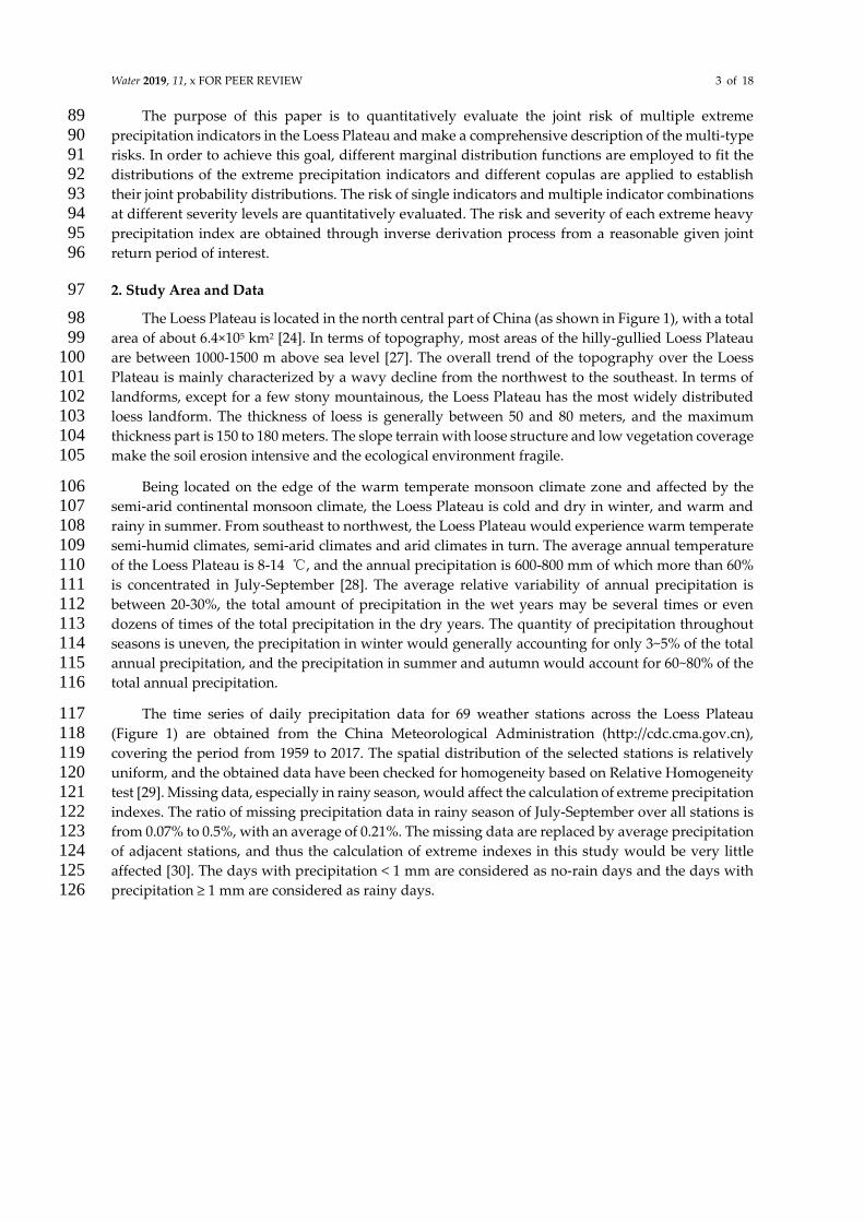
The time series of daily precipitation data for 69 weather stations across the Loess Plateau 117 (Figure 1) are obtained from the China Meteorological Administration (http://cdc.cma.gov.cn), 118 covering the period from 1959 to 2017. The spatial distribution of the selected stations is relatively 119 uniform, and the obtained data have been checked for homogeneity based on Relative Homogeneity 120 test [29]. Missing data, especially in rainy season, would affect the calculation of extreme precipitation 121 indexes. The ratio of missing precipitation data in rainy season of July-September over all stations is 122 from 0.07% to 0.5%, with an average of 0.21%. The missing data are replaced by average precipitation 123 of adjacent stations, and thus the calculation of extreme indexes in this study would be very little 124 affected [30]. The days with precipitation < 1 mm are considered as no-rain days and the days with 125 precipitation ≥ 1 mm are considered as rainy days. 126

Water 2019, 11, x FOR PEER REVIEW 4 of 18

127

Figure 1. Geographical location and 69 meteorological stations of the Loess Plateau. 128

3. Method 129

3.1. Marginal distribution and univariate return period 130

To quantify the probabilistic feature for a particular random variable, on account of the selection 131 criteria, the marginal distribution is usually constructed by choosing the best fitted distribution 132 among a set of pre-assigned distributions such as Pearson type III (P3), lognormal (LN), Log Pearson 133 type III (LP III) [20,31]. In this study, the general extreme value (GEV) distribution, Gamma, P3, LN, 134 LP III and Weibull distributions are the candidate models which are applied to quantify the 135 probabilistic characteristics for different extreme precipitation indicators. The unknown marginal 136 distribution parameters are estimated through the maximum likelihood estimation (MLE) method. 137 The root mean square error (RMSE), Kolomogorov-Smirnov (KS) test and Akaike’s information 138 criteria (AIC, [32]) are used for testing and selecting the best fitted marginal distribution among the 139 pre-assigned marginal distributions. The AIC and RMSE can be obtained as follows 140

=

+=

−=

MSERMSE

kMSENAIC

xxN

MSEN

i

o

i

e

i

2)log(*

)(1 2

(1) 141

where MSE is the mean square error, N is the length of the random variable; k represents the number 142

of the unknown parameters in the distribution models; e

ix denote the theoretical values obtained 143

from the fitted distribution; o

ix stands for the non-exceedance probabilities derived from the 144

Gringorten plotting position formula [33] which is expressed as: 145

12.0

44.0)(

+

−=

N

llLP (2) 146

where l stands for the lth smallest observation and the observations are arranged in an ascending 147 order. 148

Water 2019, 11, x FOR PEER REVIEW 5 of 18

Once the marginal distributions are fitted for the extreme precipitation indicators, the risk of 149 extreme precipitation indices can be quantitatively assessed based on the univariate return period 150 (RP). The RP of an extreme precipitation index is described as the time between two consecutive 151 events. The formula of single variable return period that used in this study is shown as: 152

=

−=

)(

1

)(1

1

2

1

xFT

xFT

(3) 153

where F(x) is the cumulative distribution functions (CDF) of precipitation indicator and ranges 154

between 0 and 1; 1T / 2T represents the RP of precipitation indicator with value greater/less than or 155

equal to a certain value of x. 156

3.2. Construction of joint distribution of extreme precipitation indicators 157

In reality, precipitation events tend to show diverse characteristics, which are described by 158 different indicators. Also, these indicators of precipitation always have correlation in different 159 degrees. The separated analysis of multiple indicators often can neither reveal the correlation among 160 them, nor quantify the joint risk of the correlated indicators. In this study, copula functions are 161 considered to build interdependence relationships between different precipitation indicators. The 162 copulas are powerful techniques which can flexibly construct multivariate joint distribution based on 163 the marginal distributions of related variables. Based on the theory of copula function proposed by 164 Sklar [34], the joint probability distribution of two correlated random variables can be expressed as 165 [35]: 166

( , ) ( ( ), ( ))X YF x y C F x F y= (4) 167

where x, y are the values of random variables X and Y, respectively; FX and FY refer to marginal CDFs 168 of the random vector (X, Y). A copula function C exists when the marginal distributions are 169 continuous and it can be expressed as [36]: 170

1 1( , ) ( ( ), ( ))C u v F F u F v− −= (5) 171

where u = F(x) and v = F(y), (u, v ∈ [0, 1]). Nelsen [35] gives more details on the characteristics of 172 copulas. 173

Many copula families, including elliptical, Archimedean, and extreme value copulas can be 174 applied in practical multivariate analysis. The well-known Gaussian copula, t copula which belong 175 to elliptical family and four Archimedean copulas (Joe, Gumbel, Clayton, and Frank) are adopted in 176 this study [37]. These copulas are employed due to their capabilities of capturing various kind of 177 dependence structures. In case of the precipitation indicators, different precipitation indices show 178 distinct relationships (positively or negatively correlated) and the chosen copulas are able to reflect 179 these complex interrelationships [21]. The parameters of copula functions are estimated through the 180 MLE approach. The KS test, AIC and RMSE measures are then used for testing and selecting the best 181 fitted copula. 182

3.3. Bivariate return periods of extreme precipitation indicators 183

The mathematical calculation of RP for single variable is given in Equation 3, which is used to 184 calculate the theoretical recurrence time periods for each precipitation index corresponding to 185 different severity. For multiple correlated variables, once the marginal distributions and joint 186 distributions are obtained, the joint RPs can be estimated based on the different combination types of 187 the variables. Salvadori and de Michele [38] have introduced and discussed the concept of bivariate 188

Water 2019, 11, x FOR PEER REVIEW 6 of 18

RPs. In this study, the following three kinds of joint RPs are investigated for different combinations 189 of correlated variables: 190

),(1

1

),()()(1

1

),x(

1,x

vuCvu

yxFyFxFyYXPT yYX

+−−=

+−−=

=

(6) 191

),(1

1

),(1

1

)or x (

1or x

vuCyxFyYXPT yYX

−=

−=

=

(7) 192

),(

1

),()(

1

)x,(

1x,

vuCvyxFyFyYXPT yYX

−=

−=

=

(8) 193

where T{X>x,Y>y} represents the bivariate RP when both X and Y exceeding the specific values (i.e. 194 X ≥ x and Y ≥ y); T{X>x or Y≥y} denotes the RP with X exceeding the threshold of x or Y exceeding the 195 threshold of y. T{X>x,Y≤y} represents the joint RP of the event that X is higher than a certain threshold 196 x and Y is smaller than and equal to a certain value y. 197

It is worthy to notice that previous studies have often calculated the joint risk using specific 198 values of marginal CDFs and thus the calculated joint RPs of all stations in the region are often too 199 small or too large. Excessive return periods often indicate that the critical events under current 200 selected severity are extremely unlikely to happen or the results are not credible because the CDF 201 values are too close to the tail. Although a very small bivariate RP indicates that the event is at a high 202 risk of joint occurrence, it cannot provide the severity of the event corresponding to a larger joint 203 recurrence period within a reasonable range, and thus may underestimate the severity of the joint 204 risk. In this case, the severity of the event should be quantitatively estimated under a selected joint 205 return period. Here the inverse calculation processes corresponding to Equation 6-8 are respectively 206 shown as: 207

yYXTvuCvu

−=+,x

11),(-

(9) 208

yYXT

vuC

−=or x

11),( (10) 209

yYXT

vuCv

=−x,

1),( (11) 210

As can be seen from the formulas above, in the case when the joint RPs are known, the right side of 211 the formulas can be known and infinite combinations of u and v can then be obtained. In the case the 212 univariate return periods are set equal to each other, the fixed marginal CDF values can be derived 213 based on golden section search and parabolic interpolation method [39]. The univariate return period 214 and the specific variable values corresponding to the marginal distributions can then be calculated. 215

4. Method Application and Results Analyses 216

To quantify the multiple characteristics of extreme precipitation in the study area, a set of 217 suitable indices are desired. Many candidate extreme precipitation indices have been used in the past 218 research works [40]. Considering the fact that precipitation in the Loess Plateau is generally low but 219 concentrated in the rainy season, the selected indicator set is expected to contain both indices that 220 could describe the severity of drought and indices that could reflect extreme heavy rainfall. For the 221 objective of this, the potential indices of the amount of extreme heavy precipitation (P95), the days 222

Water 2019, 11, x FOR PEER REVIEW 7 of 18

with extreme precipitation (D95) and the intensity of extreme heavy precipitation (I95) are used to 223 reflect extreme heavy rainfall. The continuous dry days (CDD) would be selected as the index to 224 reflect the degree of drought. In addition, the annual total precipitation PRTOT is also chosen because 225 it can flexibly reflect the degree of drought and humidity of the climate. These chosen indicators have 226 been widely used in the study of precipitation extremes. Detailed definitions of the five precipitation 227 indices are shown in Table 1. 228

Table 1. Definitions of five precipitation indices that used in the study. 229

Indices Abbreviations Definitions Unit

PRTOT PRTOT The amount of annual total precipitation mm

Number of extreme

heavy precipitation

days

D95 Number of days with precipitation exceeding the

95th percentile of precipitation series (daily

precipitation ≥ 1 mm) during 1971–2000.

days

The amount of

extreme heavy

precipitation

P95 Annual total amount of precipitation with daily

precipitation exceeding the 95th percentile of

precipitation series during 1971–2000

mm

The intensity of

extreme heavy

precipitation

I95 Mean daily precipitation intensity of extreme

heavy precipitation

mm/day

Consecutive dry

days

CDD Maximum number of consecutive dry days (days

with precipitation < 1 mm)

days

230

4.1. Univariate analysis 231

After calculating the results of the five selected precipitation indices for each station, the 232 marginal distributions of those precipitation indices would be constructed. Taking Qindu station as 233 an example, the best fitted marginal distributions for the five indices, including the parameter values 234 of each fitted distribution, KS test results, RMSE and AIC values are shown in Table 2. It can be seen 235 from the table that PRTOT, P95 and D95 are all fitted by the LP III distribution, I95 is fitted with GEV 236 distribution, and gamma distribution is more suitable for CDD index. From the p values of KS test 237 results, it can be concluded that all fitted distributions prove to be effective in describing the 238 probabilistic features of the indicators (with p > 0.05). The graph-based verification method is used: 239 Figure 2 compares the theoretical cumulative probability distribution to the empirical cumulative 240 probability distribution for each indicator. This figure shows that the fitted CDF curves of the five 241 indexes are very close to the observed values. For some indicators, we focus on the analysis of their 242 upper tail performance (the top right end of the curve), such as I95, D95, P95, and CDD, because the 243 closer the corresponding events of these indicators are to the upper tail end, the more serious these 244 events are. PRTOT is a comprehensive evaluation index. The events close to the upper tail indicate 245 that the annual precipitation is abundant, while the events close to the lower tail indicate that the 246 annual precipitation is less. However, each fitting distribution performs well in the tail of interest, 247 which shows that the risk inference results of extreme cases (high recurrence time period events) 248 according to different indicators in the study are reliable. 249

Table 2. Statistical test results for marginal distribution of five precipitation indices of Qindu station. 250

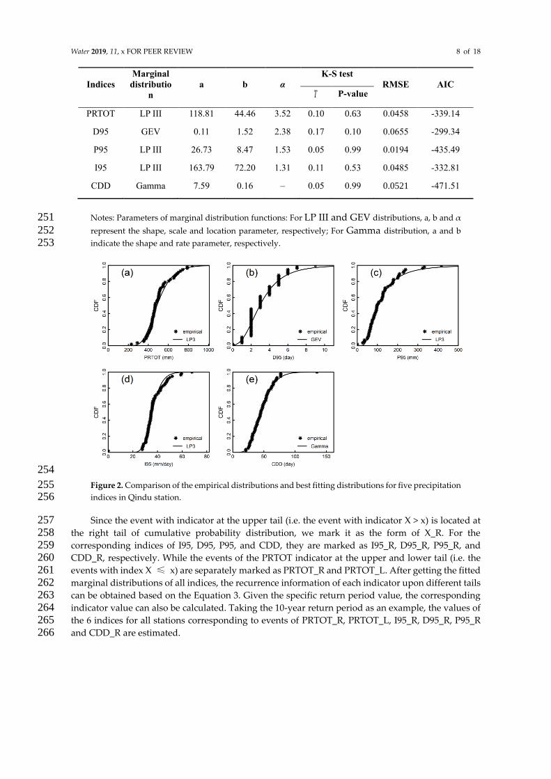
Water 2019, 11, x FOR PEER REVIEW 8 of 18

Indices

Marginal

distributio

n

a b α

K-S test

RMSE AIC T P-value

PRTOT LP III 118.81 44.46 3.52 0.10 0.63 0.0458 -339.14

D95 GEV 0.11 1.52 2.38 0.17 0.10 0.0655 -299.34

P95 LP III 26.73 8.47 1.53 0.05 0.99 0.0194 -435.49

I95 LP III 163.79 72.20 1.31 0.11 0.53 0.0485 -332.81

CDD Gamma 7.59 0.16 – 0.05 0.99 0.0521 -471.51

Notes: Parameters of marginal distribution functions: For LP III and GEV distributions, a, b and α 251

represent the shape, scale and location parameter, respectively; For Gamma distribution, a and b 252 indicate the shape and rate parameter, respectively. 253

254

Figure 2. Comparison of the empirical distributions and best fitting distributions for five precipitation 255 indices in Qindu station. 256

Since the event with indicator at the upper tail (i.e. the event with indicator X > x) is located at 257 the right tail of cumulative probability distribution, we mark it as the form of X_R. For the 258 corresponding indices of I95, D95, P95, and CDD, they are marked as I95_R, D95_R, P95_R, and 259 CDD_R, respectively. While the events of the PRTOT indicator at the upper and lower tail (i.e. the 260 events with index X ≤ x) are separately marked as PRTOT_R and PRTOT_L. After getting the fitted 261 marginal distributions of all indices, the recurrence information of each indicator upon different tails 262 can be obtained based on the Equation 3. Given the specific return period value, the corresponding 263 indicator value can also be calculated. Taking the 10-year return period as an example, the values of 264 the 6 indices for all stations corresponding to events of PRTOT_R, PRTOT_L, I95_R, D95_R, P95_R 265 and CDD_R are estimated. 266

Water 2019, 11, x FOR PEER REVIEW 9 of 18

267

Figure 3. The values of 6 marked indexes at 10-year return period over the the Loess Plateau. 268

Figure 3 shows the computational results of 6 marked indices at 10-year return period over the 269 Loess Plateau in the form of interpolation maps with contour lines. The color gradients are utilized 270 to visually distinguish the differences of each indicator in different regions. Due to the spatial 271 transition characteristics of precipitation over the Loess Plateau, Figure 3a-e shows a gradient 272 increasing trend from northwest to southeast in the Loess Plateau, while Figure 3f (CDD_R) shows a 273 gradient decreasing trend. The differences of 10-year return period values between PRTOT_R and 274 PRTOT_L vary greatly, which shows a range of 127-373 mm at different stations and an average 275 difference of 265 mm over the whole region. The PRTOT_R in the arid area can even reach 3.03 times 276 higher than PRTOT_L. The comparison of P95_R and PRTOT_L shows that the extreme rainfall in 277 wet year is only slightly lower than the annual precipitation in the dry year. The minimum value of 278 I95_R appears in the high mountain area of the southwestern Loess Plateau, while in the northwest 279 region with the least annual precipitation, the I95_R is merely slightly lower than the southeast region 280 with the most precipitation. In addition, the value of D95_R in the northwest region is very low, 281 which indicates that the annual precipitation in Northwest China may be highly concentrated in 282 several heavy rainfall events and makes the region into severe drought for most of the year. This 283 conclusion can also be obtained from the performance of CDD_R in this area, the duration of 284 continuous drought of 10-year return period can even reach 160 days. 285

286

Water 2019, 11, x FOR PEER REVIEW 10 of 18

Table 3. The indicator combinations with their definitions. 287

ID Combinations Return periods

(years) Variables (X, Y)

1 {PRTOT_L, CDD_R} T{X≤x and Y>y} PRTOT, CDD

2 {PRTOT_R, CDD_R} T{X>x and Y>y} PRTOT, CDD

3 {D95_R, P95_R} T{X>x and Y>y} D95, P95

4 {P95_R, I95_R} T{X>x and Y>y} P95, I95

5 {P95_R or I95_R} T{X>x or Y>y} P95, I95

6 {P95_R, CDD_R} T{X>x and Y>y} P95, CDD

4.2. Bivariate Analysis 288

The combined events of X and Y are denoted as {X, Y} and {X or Y}, which respectively represents 289 the concurrence of X and Y events, and the occurrence of X or Y event. The recurrence periods of the 290 two combinations are labeled as T{X, Y} and T{X|Y}, respectively. For the five climate indicators, the joint 291 performance of six combinations are studied, namely {PRTOT_L, CDD_R}, {PRTOT_R, CDD_R}, 292 {D95_R, P95_R}, {P95_R, I95_R}, {P95_R or I95_R} and {P95_R, CDD_R}. The definitions of joint RPs 293 of precipitation indicators are listed in Table 3. T{PRTOT_L, CDD_R} indicates the joint return period of 294 PRTOT less than and equal to a specific value and CDD exceed its specific threshold, which means a 295 long period of continuous drought appears in a dry year. T{PRTOT_R, CDD_R} denotes the joint RP of long-296 term continuous drought occurs even when the annual precipitation is sufficient, indicating 297 consecutive PRTOT and CDD exceed their specific thresholds simultaneously. {D95_R, P95_R} 298 indicates a strong precipitation event with the precipitation amount and precipitation duration 299 exceed their specific thresholds. {P95_R, I95_R} / T{P95_R | I95_R} signifies an extreme heavy 300 precipitation event in which precipitation and / or precipitation intensity exceeds the thresholds. As 301 a combination of extreme heavy precipitation and continuous drying indicators, {P95_R, CDD_R} 302 implies the concurrence of floods and droughts in the same year. 303

It can be seen from Table 3 that although joint RPs of six indicator combinations are going to be 304 addressed, only the joint probability distributions of four combinations need to be quantified, namely 305 {PRTOT,CDD},{D95, P95}, {P95, I95}, and {P95, CDD} (see last column). By using the best fitted 306 marginal distribution functions, the joint probability distributions of four combinations can then be 307 obtained by copulas. The KS test and the indices of RMSE，AIC are also applied to select the best 308 performed copulas for different indicator combinations. Four bivariate CDF graphics based on the 309 best fitted copulas at Qindu Station are presented in Figure 4. The numerical variation ranges of the 310 two indicators for each combination is given on the x-axis and the y-axis, and the [0, 1] interval of the 311 joint CDF is given on the z-axis. 312

313

Water 2019, 11, x FOR PEER REVIEW 11 of 18

314

Figure 4. Joint CDFs based on the best fitted copulas for four indicator combinations of 315 {PRTOT,CDD},{D95, P95}, {P95, I95}, and {P95, CDD} at Qindu Station. 316

According to Equations (6)-(8), the value of return period is determined by two dependent 317 variables, and thus it is possible to get the same return period value with different combinations of 318 the variables. Figure 5 shows the contour maps of the joint return period of 5, 10, 20, 50 and 100 years 319 under different combinations of six precipitation indicators. We can quantitatively reflect the joint 320 risk of simultaneous occurrence of different precipitation extremes corresponding to their numerical 321 combinations. Each index gradually tends to be less likely to occur along the direction of increasing 322 joint return period, that is, the return period of single variable in this direction also gradually 323 increases. It can be seen from the figure that the contour line of recurrence period presents three 324 different forms: Figure 5a is obtained by Equation (8), and the joint recurrence period gradually 325 increases in the direction in which the PRTOT tends to the lower tail and the CDD tends to the upper 326 tail. Figure 5(b-d and f) are achieved through the Equation (6) and the joint RP of each group would 327 gradually increase in the direction of the upward tail of both variables. Figure 5e is obtained from 328 Equation (7). Compared with Figure 4, it can be seen that for two climate indicators with same 329 numerical combination, Figure 5e always shows a smaller return period, that is, the events with 330 relationship of 'or' is more likely to occur. 331

Water 2019, 11, x FOR PEER REVIEW 12 of 18

332

Figure 5. The joint return period of 5, 10, 20, 50 and 100 years under different combinations of six 333 climate indicators. 334

Figure 6 shows the joint RPs of each combination group under the condition of given 10-year 335 return periods for two single indicators (corresponding to Figure 3). Figure (6a) to Figure (6f) 336 respectively denote the six combinations of ID1-ID6 in Table 3 and the values of the recurrence 337 periods vary directly proportional to the size of the solid circles in the figure. By comparing the joint 338 return periods of Figure 6a with Figure 6b, it can be seen that the return period values of Figure 6b 339 are always larger (58.5 years larger on average) than that of Figure 6a. The results of the study area 340 as a whole are consistent with our general perception that wet years are less prone to prolonged 341 continuous drought. It is worthy to notice that there are still 17 stations with T{PRTOT_L, CDD_R} larger 342 than T{PRTOT_R, CDD_R}. This is because the annual precipitation of these stations is more concentrated in 343 few extreme precipitation events, and CDD is less affected by the annual precipitation, and thus the 344 two precipitation indicators even show a certain degree of negative correlation. 345

From the spatial distribution of RPs, the size of the circles in Figure 6a and Figure 6b in the whole 346 region is basically opposite, which means that the events of {PRTOT_L, CDD_R} are hard to happen 347 at the stations where the events of {PRTOT_R, CDD_R} are relatively easy to occur. The spatial 348 distribution of circles of different sizes in Figure 6f is similar to that in Figure 6b, that is, the events of 349 {PRTOT_R, CDD_R} and {P95_R, CDD_R} show some degree of convergence. This is because the 350 annual precipitation for this condition is too concentrated. Figure 6(c-e) show the joint return periods 351 of different combinations of the three extreme heavy precipitation indicators. The corresponding joint 352 return periods are all relatively smaller than other combinations, which is because the three indicators 353 are strongly correlated. 354

Water 2019, 11, x FOR PEER REVIEW 13 of 18

355

Figure 6. The joint returns periods of each combination group under the condition of 10-year return 356 periods of two single indicators. Figure 6 a-e represent six combinations of events: {PRTOT_L, 357 CDD_R}, {PRTOT_R, CDD_R}, {D95_R, P95_R}, {P95_R, I95_R}, {P95_R or I95_R} and {P95_R, CDD_R}. 358

The average return periods of all stations in Figure 6a, 6b, and 6f are 85.2, 143.8, and 126.2, 359 respectively. These results demonstrate that the three compound events with two indicators 360 corresponding to the 10-year return period are difficult to occur simultaneously in the same year. 361 However, the quantitative calculation results are greatly affected by the selection of different models 362 since the joint probabilities of these events are very close to the tails, which suggest that the 363 quantitative results will show great uncertainty. Correspondingly, the joint RP values of Figure 6c-e 364 are too small to exhibit their extreme risk situations, especially for Figure 6c and Figure 6e. This 365 requires a balance that allows the assessment to calculate the degree of extreme risk that may occur 366 within its credible return periods. For the time series of precipitation data used in this paper is about 367 60 years, the return period of individual extreme indicators with a joint RP of 50 years corresponding 368 to Figure 6c-e are considered to be calculated. Under the condition of two univariate return period 369 values are set to be equal to each other, by using Equations 9-11, and then the specific values for each 370 individual indicator (Figure 7) and the corresponding return periods (Figure 8) are obtained. 371

Water 2019, 11, x FOR PEER REVIEW 14 of 18

372

Figure 7. The specific values for each individual indicator under joint return period of 50 years 373 corresponding to 3 combination groups: Figure 7 a1 and Figure 7 a2 are corresponding to {D95_R, 374 P95_R} event; Figure 7b1 and Figure 7 b2 are corresponding to {P95_R, I95_R} event; Figure 7 c1 and 375 Figure 7 c2 are corresponding to {P95_R or I95_R} event. 376

Figure 7(a1) and 7(a2) are individually the interpolation maps of D95 and P95 with the joint 377 return period of 50 years for events of {D95_R, P95_R}. The results show that spatial distribution of 378 the two indicators is very similar to each other, and the overall values are higher than the values of 379 the 10-year return period in Figure 3. The corresponding return period of single variable ranges from 380 15.7 to 44.4 years, with an average of 29.1 years (Figure 8a). Similarly, Figures 7(b1,b2)-8(b) and 381 7(c1,c2)-8(c) show the respective indicator values in the events of {P95_R, I95_R} and {P95_R or I95_R}, 382 respectively. It can be seen that the indicator values of {P95_R or I95_R} events are much higher than 383 those of {P95_R, I95_R} events, in which the P95 is 112.3 mm higher on average, and I95 is 19.9 384 mm/day higher on average. The return periods of P95_R and I95_R in events of {P95_R or I95_R} are 385 close to 100 year. In terms of probability, the 100-year RP of the P95 event or the 100-year RP of the 386 I95 event can be encountered in 50 years. Heavy rainfall events are especially serious in the south and 387 northeast of the Loess Plateau. The station with the most amount of extreme heavy rainfall shows a 388 P95 of 931 mm, and the I95 is 97 mm/day. 389

Water 2019, 11, x FOR PEER REVIEW 15 of 18

390

Figure 8. The univariate return period values for each individual indicator under joint return period 391 of 50 years corresponding to 3 combination groups: Figure 8 a1 and Figure 8 a2 are corresponding to 392 {D95_R, P95_R} event; Figure 8b1 and Figure 8 b2 are corresponding to {P95_R, I95_R} event; Figure 393 8 c1 and Figure 8 c2 are corresponding to {P95_R or I95_R} event. 394

5. Conclusions and Discussions 395

Based on the daily precipitation data of past six decades, the probability characteristics of five 396 extreme precipitation indices in the Loess Plateau are studied. Moreover, the joint risk of different 397 combinations of precipitation indexes is quantitatively evaluated. Specifically, six marginal 398 distribution functions are applied to fit each precipitation index and six copula models belonging to 399 the elliptic copula and Archimedes copula family are selected to fit the joint distributions of six 400 indicator combinations. The RMSE, AIC, KS test were used to evaluate the performance of marginal 401 and joint distributions. The index values corresponding to the 10-year return period of each 402 precipitation indicator are calculated, and the joint return periods of all combinations under the 403 condition of 10-year return period for single variables are calculated. Finally, the indicator values 404 with their RPs of three extreme heavy precipitation index combinations are calculated under the 405 condition of 50-year joint return period. 406

Main findings of the present study are summarized as follows: The study of single indicators 407 shows that the extreme precipitation in wet years is almost equal to the annual precipitation in dry 408 years over the Loess Plateau. The Northwest Loess Plateau with least amount of annual precipitation 409 shows extreme precipitation intensity is only slightly lower than that in humid southwest area. It is 410 also found that the T{PRTOT_L, CDD_R} is greater than T{PRTOT_R, CDD_R} at 17 stations, which is also because 411 the precipitation of these stations is mostly concentrated in a few extreme precipitation events, while 412 CDD is less affected by the annual precipitation, and the two precipitation indicators even show a 413 certain degree of negative correlation. In terms of probability, P95 or I95 event of 100-year level can 414 be encountered in 50-year return period over the Loess Plateau. The precipitation amount and 415

Water 2019, 11, x FOR PEER REVIEW 16 of 18

intensity of the Loess Plateau vary greatly in spatial distribution. The 10-year return period in the 416 northwestern region can occur for more than five months with no precipitation events. In the 417 southeastern region, there are foreseeable long-term extreme precipitation events. 418

Previous studies on the risk assessment of extreme precipitation often ignored the correlated 419 characteristics of different precipitation indicators and could not quantitatively evaluate the joint risk 420 of different indicators. Few studies have analyzed the joint risks of different indicators, however they 421 are all aimed at the forward calculation process, that is, by giving fixed indicator values of certain 422 recurrence periods to calculate the joint return period. The disadvantage of this scheme is that the 423 obtained joint return periods always tend to be too small or too large. Too small a recurrence period 424 does not reflect the severity of the event, and too large a recurrence period means that event is very 425 close to the tail of the distribution and the result is unreliable. In this study, the univariate and joint 426 risks of different extreme precipitation indexes in the Loess Plateau are synthetically studied by 427 forward and reverse calculations, and the RPs of univariate indicators based on joint RPs of 50 years 428 is calculated. 429

The Loess Plateau is located on the edge of different climatic regions, which results in the serious 430 imbalance of the spatial and temporal distribution of precipitation. The annual precipitation in the is 431 highly concentrated in rainy seasons, which makes the region in a serious drought state for most of 432 the year, especially for the northwest region, while the Southwest Loess Plateau is prone to very 433 heavy rainfall. Therefore, it is necessary to develop effective management plan for water resources 434 system and environment. A systematic plan for water storage in flood season and water resources 435 allocation in dry season is essentially needed. 436

437

Acknowledgements: This research was supported by the National Key Research and Development Plan 438 (2016YFA0601502), the Natural Sciences Foundation (51520105013, 51679087), the 111 Program (B14008), the 439 Natural Science and Engineering Research Council of Canada and the Fundamental Research Funds for the 440 Central Universities (2016XS89). 441

References 442

1. IPCC, Climate change 2007: The physical science basis. Contribution of Working Group I to the Fourth 443 Assessment Report of the Intergovernmental Panel on Climate Change, Cambridge Univ. Press, 2007, 444 Cambridge, U.K. and New York. 445

2. IPCC, Climate Change 2014: Impacts, Adaptation, and Vulnerability: Contribution to the Fifth Assessment 446 Report of the Intergovernmental Panel on Climate Change. Cambridge University Press, 2014, Cambridge, 447 UK. and New York, NY. 448

3. Kharin, V,V,, Zwiers F.W., Zhang, X, et al. Changes in Temperature and Precipitation Extremes in the 449 CMIP5 Ensemble. Climatic Change, 2013, 119(2). 450

4. Barros, V., Stocker, T.F. Managing the risks of extreme events and disasters to advance climate change 451 adaptation : special report of the Intergovernmental Panel on Climate Change. Journal of Clinical 452 Endocrinology & Metabolism, 2012, 18(6):586-599. 453

5. Chang, L.C., Chang, F.J.. Intelligent control for modelling of real-time reservoir operation. Hydrological 454 Processes, 2010, 15(9): 1621–1634 455

6. Jhong, B.C. & Tung, C.P. Evaluating Future Joint Probability of Precipitation Extremes with a Copula-Based 456 Assessing Approach in Climate ChangeWater Resour Manage 2018, 32(13), 4253-4274. 457

7. Kharin, V.V., Zwiers, F.W., Zhang, X., and Wehner M. Changes in Temperature and Precipitation Extremes 458 in the CMIP5 Ensembl. Climatic Change, 2013, 119(2). 459

Water 2019, 11, x FOR PEER REVIEW 17 of 18

8. Caesar, J., Alexander, L.V., Trewin, B., et al. Changes in temperature and precipitation extremes over the 460 Indo-Pacific region from 1971 to 2005. Int J Climatol, 2011, 31(6):791–801 461

9. You, Q., Kang, S., Aguilar, E., Pepin, N., Wolfgang-Albert Flügel, & Yan, Y. Changes in daily climate 462 extremes in china and their connection to the large scale atmospheric circulation during 1961–2003. Climate 463 Dynamics, 2011, 36(11-12), 2399-2417. 464

10. Zhai, P.M., Zhang, X.B., Wan, H., and Pan, X.H. Trends in total precipitation and frequency of daily 465 precipitation extremes over China. Journal of Climate, 2005, 18: 1096–1108 466

11. Wang, C., Ren, X., Li, Y. Analysis of extreme precipitation characteristics in low mountain areas based on 467 three-dimensional copulas—taking Kuandian County as an example[J]. Theoretical and Applied 468 Climatology, 2017, 128(1-2):169-179. 469

12. Wahl, T., Jain, S., Bender, J., Meyers, S.D., & Luther, M.E. Increasing risk of compound flooding from storm 470 surge and rainfall for major us cities. Nature Climate Change, 2015. 471

13. Madadgar, S., Aghakouchak, A., Farahmand, A., & Davis, S.J. Probabilistic estimates of drought impacts 472 on agricultural production. Geophysical Research Letters, 2017, 44(15), 7799-7807. 473

14. Zhang, D.D., Yan, D.H., Lu, F., Wang, Y.C., & Feng, J. Copula-based risk assessment of drought in yunnan 474 province, china. Natural Hazards, 2015, 75(3), 2199-2220. 475

15. Rana, A., Moradkhani, H., & Qin, Y. Understanding the joint behavior of temperature and precipitation for 476 climate change impact studies. Theoretical & Applied Climatology, 2016, 129(1), 1-19. 477

16. Jeong, D.I., Sushama, L., Khaliq, M.N., & René Roy. A copula-based multivariate analysis of canadian rcm 478 projected changes to flood characteristics for northeastern canada. Climate Dynamics, 2014, 42(7-8), 2045-479 2066. 480

17. Qian, L., Wang, H., Dang, S., Wang, C., Jiao, Z., & Zhao, Y. Modelling bivariate extreme precipitation 481 distribution for data-scarce regions using gumbel-hougaard copula with maximum entropy estimation. 482 Hydrological Processes. 2017. 483

18. Salvadori, G. , & De Michele, C. Multivariate real-time assessment of droughts via copula-based multi-site 484 hazard trajectories and fans. Journal of Hydrology, 2015, 526, 101-115. 485

19. Volpi, E., & Fiori, A. Hydraulic structures subject to bivariate hydrological loads: return period, design, 486 and risk assessment. Water Resources Research, 2014, 50(2), 885-897. 487

20. Fan, Y.R., Huang, W.W., Huang, G.H., et al. Bivariate hydrologic risk analysis based on a coupled entropy-488 copula method for the Xiangxi River in the Three Gorges Reservoir area, China. Theoretical and Applied 489 Climatology, 2016, 125(1-2):381-397. 490

21. Zhang, Q., Li, J., Singh, V.P, & Xu, C.Y. Copula-based spatio-temporal patterns of precipitation extremes 491 in china. International Journal of Climatology, 2013, 33(5), 1140-1152. 492

22. Goswami, U.P., Hazra, B., & Kumar, G.M. Copula-based probabilistic characterization of precipitation 493 extremes over north sikkim himalaya. Atmospheric Research, 2018, S016980951830098X-. 494

23. Wang, L., Cheung, K. K. W., Chi-Yung Tam, Tai, A.P.K., & Li, Y. Evaluation of the regional climate model 495 over the loess plateau of china. International Journal of Climatology, 2018, 38. 496

24. Xin, Z., Yu, X., Li, Q., & Lu, X.X. Spatiotemporal variation in rainfall erosivity on the chinese loess plateau 497 during the period 1956–2008. Regional Environmental Change, 2011, 11(1), 149-159. 498

25. Liu, Q., & Yang, Z. Quantitative estimation of the impact of climate change on actual evapotranspiration 499 in the yellow river basin, china. Journal of Hydrology 2010, 395(3-4), 226-234. 500

Water 2019, 11, x FOR PEER REVIEW 18 of 18

26. Li, Z., Zheng, F.L., Liu, W.Z., & Jiang, D.J. Spatially downscaling gcms outputs to project changes in 501 extreme precipitation and temperature events on the loess plateau of china during the 21st century. Global 502 and Planetary Change, 2012, 82-83(none), 0-73. 503

27. Nolan, S., Unkovich, M., Yuying, S., Lingling, L., & Bellotti, W. Farming systems of the loess plateau, gansu 504 province, china. Agriculture Ecosystems & Environment, 2008, 124(1-2), 13-23. 505

28. Liang, W., Bai, D., Wang, F., Fu, B., Yan, J., & Wang, S., et al. Quantifying the impacts of climate change 506 and ecological restoration on streamflow changes based on a budyko hydrological model in china's loess 507 plateau. Water Resources Research, 2015, 51(8), 6500-6519. 508

29. Wang, X.L. (2008). Accounting for autocorrelation in detecting mean shifts in climate data series using the 509 penalized maximal t or f test. Journal of Applied Meteorology & Climatology, 47(9), 2423-2444. 510

30. Wang, W., Shao, Q., Peng, S., Zhang, Z., Xing, W., & An, G., et al. (2011). Spatial and temporal characteristics 511 of changes in precipitation during 1957–2007 in the haihe river basin, china. Stochastic Environmental 512 Research & Risk Assessment, 25(7), 881-895. 513

31. Sun, C.X., Huang, G.H., Fan, Y., Zhou, X., Lu, C., & Wang, X.Q. Drought occurring with hot extremes: 514 Changes under future climate change on Loess Plateau, China. Earth's Future, 2019, 7, 587– 604. 515

32. Akaike H. A new look at the statistical model identification. IEEE Transactions on Automatic Control, 1974, 516 19(6), 716-723. 517

33. Gringorten, Irving I . A plotting rule for extreme probability paper[J]. Journal of Geophysical Research, 518 1963, 68(3):813-814. 519

34. Sklar, K. Fonctions dé repartition á n dimensions et leurs marges. Publications de l'Institut de Statistique 520 de l'Universite dé Paris, 1959, 8:229-231. 521

35. Nelsen, R.B. An Introduction to Copulas. Springer, 2006, New York. 522

36. Sraj, M., Bezak, N., & Brilly, M. Bivariate flood frequency analysis using the copula function: a case study 523 of the litija station on the sava river. Hydrological Processes, 2015, 29(2), 225-238. 524

37. Zhou, X., Huang, G., Wang, X., Fan, Y., & Cheng, G. A coupled dynamical-copula downscaling approach 525 for temperature projections over the canadian prairies. Climate Dynamics, 2018, 51(7-8), 2413-2431. 526

38. Salvadori, G, de Michele, C . Frequency analysis via copulas: Theoretical aspects and applications to 527 hydrological events. Water Resources Research, 2004, 40(12) 1-17. 528

39. Egrioglu E , Aladag C , Basaran M . A new approach based on the optimization of the length of intervals in 529 fuzzy time series. \\ldots of Intelligent and Fuzzy \\ldots, 2011, 22(1):15-19. 530

40. G. Bürger, Murdock T Q , Werner A T , et al. Downscaling Extremes—An Intercomparison of Multiple 531 Statistical Methods for Present Climate[J]. Journal of Climate, 2012, 25(12):4366-4388. 532

41.

42. © 2019 by the authors. Submitted for possible open access publication under the

terms and conditions of the Creative Commons Attribution (CC BY) license

(http://creativecommons.org/licenses/by/4.0/).

533

534

535