
Cisco Reader Comment Card - IndigoThemes · 1 Years of networking experience Years of experience...
266
Cisco Reader Comment Card General Information 1 Years of networking experience Years of experience with Cisco products 2 I have these network types: LAN Backbone WAN Other: 3 I have these Cisco products: Switches Routers Other: Specify model(s) 4 I perform these types of tasks: H/W Install and/or Maintenance S/W Config Network Management Other: 5 I use these types of documentation: H/W Install H/W Config S/W Config Command Reference Quick Reference Release Notes Online Help Other: 6 I access this information through: Cisco Connection Online (CCO) CD-ROM Printed docs Other: 7 Which method do you prefer? 8 I use the following three product features the most: Document Information Document Title: Guide to ATM Technology Part Number: 78-6275-03 On a scale of 1–5 (5 being the best) please let us know how we rate in the following areas: Please comment on our lowest score(s): Mailing Information Company Name Date Contact Name Job Title Mailing Address City State/Province ZIP/Postal Code Country Phone ( ) Extension Fax ( ) E-mail Can we contact you further concerning our documentation? Yes No You can also send us your comments by e-mail to [email protected], or fax your comments to us at (408) 527-8089. The document was written at my technical level of understanding. The information was accurate. The document was complete. The information I wanted was easy to find. The information was well organized. The information I found was useful to my job. % % % %
Transcript of Cisco Reader Comment Card - IndigoThemes · 1 Years of networking experience Years of experience...

Cisco Reader Comment CardGeneral Information1 Years of networking experience Years of experience with Cisco products
2 I have these network types: LAN Backbone WANOther:
3 I have these Cisco products: Switches RoutersOther: Specify model(s)
4 I perform these types of tasks: H/W Install and/or Maintenance S/W ConfigNetwork Management Other:
5 I use these types of documentation: H/W Install H/W Config S/W ConfigCommand Reference Quick Reference Release Notes Online HelpOther:
6 I access this information through: Cisco Connection Online (CCO) CD-ROMPrinted docs Other:
7 Which method do you prefer?
8 I use the following three product features the most:
Document InformationDocument Title: Guide to ATM Technology
Part Number: 78-6275-03
On a scale of 1–5 (5 being the best) please let us know how we rate in the following areas:
Please comment on our lowest score(s):
Mailing InformationCompany Name Date
Contact Name Job Title
Mailing Address
City State/Province ZIP/Postal Code
Country Phone ( ) Extension
Fax ( ) E-mail
Can we contact you further concerning our documentation? Yes No
You can also send us your comments by e-mail to [email protected], or fax your comments to us at (408) 527-8089.
The document was written at my technical level of understanding.
The information was accurate.
The document was complete. The information I wanted was easy to find.
The information was well organized. The information I found was useful to my job.
% %% %

BU
SIN
ES
S R
EP
LY
MA
ILF
IRS
T-C
LA
SS
MA
IL P
ER
MIT
NO
. 46
31
SA
N J
OS
E C
A
PO
ST
AG
E W
ILL
BE
PA
ID B
Y A
DD
RE
SS
EE
AT
TN
DO
CU
ME
NT
RE
SO
UR
CE
CO
NN
EC
TIO
NC
ISC
O S
YS
TE
MS
INC
17
0 W
ES
T T
AS
MA
N D
RIV
ES
AN
JOS
E C
A 9
51
34
-98
83
NO
PO
ST
AG
EN
EC
ES
SA
RY
IF M
AIL
ED
IN T
HE
UN
ITE
D S
TA
TE
S

Guide to ATM TechnologyFor the Catalyst 8540 MSR, Catalyst 8510 MSR, andLightStream 1010 ATM Switch Routers
170 West Tasman DriveSan Jose, CA 95134-1706USAhttp://www.cisco.com
Cisco Systems, Inc.Corporate Headquarters
Tel:800 553-NETS (6387)408 526-4000
Fax: 408 526-4100
Customer Order Number: DOC-786275Text Part Number: 78-6275-03

THE SPECIFICATIONS AND INFORMATION REGARDING THE PRODUCTS IN THIS MANUAL ARE SUBJECT TO CHANGE WITHOUT NOTICE. ALL STATEMENTS, INFORMATION, AND RECOMMENDATIONS IN THIS MANUAL ARE BELIEVED TO BE ACCURATE BUT ARE PRESENTED WITHOUT WARRANTY OF ANY KIND, EXPRESS OR IMPLIED. USERS MUST TAKE FULL RESPONSIBILITY FOR THEIR APPLICATION OF ANY PRODUCTS.
THE SOFTWARE LICENSE AND LIMITED WARRANTY FOR THE ACCOMPANYING PRODUCT ARE SET FORTH IN THE INFORMATION PACKET THAT SHIPPED WITH THE PRODUCT AND ARE INCORPORATED HEREIN BY THIS REFERENCE. IF YOU ARE UNABLE TO LOCATE THE SOFTWARE LICENSE OR LIMITED WARRANTY, CONTACT YOUR CISCO REPRESENTATIVE FOR A COPY.
The Cisco implementation of TCP header compression is an adaptation of a program developed by the University of California, Berkeley (UCB) as part of UCB’s public domain version of the UNIX operating system. All rights reserved. Copyright © 1981, Regents of the University of California.
NOTWITHSTANDING ANY OTHER WARRANTY HEREIN, ALL DOCUMENT FILES AND SOFTWARE OF THESE SUPPLIERS ARE PROVIDED “AS IS” WITH ALL FAULTS. CISCO AND THE ABOVE-NAMED SUPPLIERS DISCLAIM ALL WARRANTIES, EXPRESSED OR IMPLIED, INCLUDING, WITHOUT LIMITATION, THOSE OF MERCHANTABILITY, FITNESS FOR A PARTICULAR PURPOSE AND NONINFRINGEMENT OR ARISING FROM A COURSE OF DEALING, USAGE, OR TRADE PRACTICE.
IN NO EVENT SHALL CISCO OR ITS SUPPLIERS BE LIABLE FOR ANY INDIRECT, SPECIAL, CONSEQUENTIAL, OR INCIDENTAL DAMAGES, INCLUDING, WITHOUT LIMITATION, LOST PROFITS OR LOSS OR DAMAGE TO DATA ARISING OUT OF THE USE OR INABILITY TO USE THIS MANUAL, EVEN IF CISCO OR ITS SUPPLIERS HAVE BEEN ADVISED OF THE POSSIBILITY OF SUCH DAMAGES.
Access Registrar, AccessPath, Any to Any, AtmDirector, Browse with Me, CCDA, CCDE, CCDP, CCIE, CCNA, CCNP, CCSI, CD-PAC, the Cisco logo, Cisco Certified Internetwork Expert logo, CiscoLink, the Cisco Management Connection logo, the Cisco NetWorks logo, the Cisco Powered Network logo, Cisco Systems Capital, the Cisco Systems Capital logo, Cisco Systems Networking Academy, the Cisco Systems Networking Academy logo, the Cisco Technologies logo, ConnectWay, Fast Step, FireRunner, Follow Me Browsing, FormShare, GigaStack, IGX, Intelligence in the Optical Core, Internet Quotient, IP/VC, Kernel Proxy, MGX, MultiPath Data, MultiPath Voice, Natural Network Viewer, NetSonar, Network Registrar, the Networkers logo, Packet, PIX, Point and Click Internetworking, Policy Builder, Precept, ScriptShare, Secure Script, ServiceWay, Shop with Me, SlideCast, SMARTnet, SVX, The Cell, TrafficDirector, TransPath, ViewRunner, Virtual Loop Carrier System, Virtual Service Node, Virtual Voice Line, VisionWay, VlanDirector, Voice LAN, WaRP, Wavelength Router, Wavelength Router Protocol, WebViewer, Workgroup Director, and Workgroup Stack are trademarks; Changing the Way We Work, Live, Play, and Learn, Empowering the Internet Generation, The Internet Economy, and The New Internet Economy are service marks; and ASIST, BPX, Catalyst, Cisco, Cisco IOS, the Cisco IOS logo, Cisco Systems, the Cisco Systems logo, the Cisco Systems Cisco Press logo, Enterprise/Solver, EtherChannel, EtherSwitch, FastHub, FastLink, FastPAD, FastSwitch, GeoTel, IOS, IP/TV, IPX, LightStream, LightSwitch, MICA, NetRanger, Post-Routing, Pre-Routing, Registrar, StrataView Plus, Stratm, TeleRouter, and VCO are registered trademarks of Cisco Systems, Inc. or its affiliates in the U.S. and certain other countries. All other trademarks mentioned in this document are the property of their respective owners. The use of the word partner does not imply a partnership relationship between Cisco and any of its resellers. (9912R)
Guide to ATM Technology for the Catalyst 8540 MSR, Catalyst 8510 MSR, and LightStream 1010 ATM Switch RoutersCopyright © 1999-2000, Cisco Systems, Inc.All rights reserved.

C O N T E N T S
Preface xv
Purpose xv
Audience xv
New and Changed Information xv
Organization xvi
Related Documentation xvii
Conventions xvii
Cisco Connection Online xvii
Documentation CD-ROM xviii
C H A P T E R 1 ATM Technology Fundamentals 1-1
What is ATM? 1-1
ATM Basics 1-2
ATM Cell Basic Format 1-2
ATM Device Types 1-2
ATM Network Interface Types 1-3
ATM Cell Header Formats 1-4
ATM Services 1-5
Virtual Paths and Virtual Channels 1-5
Point-to-Point and Point-to-Multipoint Connections 1-6
Operation of an ATM Switch 1-9
The ATM Reference Model 1-11
ATM Addressing 1-12
Traffic Contracts and Service Categories 1-12
The Traffic Contract 1-13
The Service Categories 1-13
Service-dependent ATM Adaptation Layers 1-14
Common Physical Interface Types 1-15
iiiGuide to ATM Technology
78-6275-03

Contents
C H A P T E R 2 ATM Signaling and Addressing 2-1
Signaling and Addressing Overview 2-1
Signaling 2-1
Connection Setup and Signaling 2-2
ATM Signaling Protocols—UNI and NNI 2-3
Addressing 2-4
ATM Address Formats 2-4
Choosing an Address Format 2-6
Addressing on the ATM Switch Router 2-6
Autoconfigured ATM Addressing Scheme 2-7
Default Address Format Features and Implications 2-8
ILMI Use of the ATM Address 2-9
ILMI Considerations for ATM Address Migration 2-9
Additional ILMI Functions 2-9
PNNI Use of the ATM Address 2-10
LAN Emulation Use of the ATM Address 2-10
Manually Configured ATM Addresses 2-10
Signaling and E.164 Addresses 2-11
E.164 Address Conversion Options 2-12
The E.164 Gateway Feature 2-12
The E.164 Address Autoconversion Feature 2-13
The E.164 Address One-to-One Translation Table Feature 2-16
Obtaining Registered ATM Addresses 2-17
Special Signaling Features 2-18
Closed User Group Signaling 2-18
Multipoint-to-Point Funnel Signaling 2-21
C H A P T E R 3 ATM Network Interfaces 3-1
Configuration of Interface Types 3-1
ATM Network Interfaces Example 3-2
UNI Interfaces 3-3
NNI Interfaces 3-4
IISP Interfaces 3-5
ivGuide to ATM Technology
78-6275-03

Contents
C H A P T E R 4 Virtual Connections 4-1
Understanding ATM Virtual Connections 4-1
Types of Virtual Connections 4-2
Transit and Terminating Connections 4-2
Connection Components 4-2
Autoconfigured Parameters of Virtual Connections 4-3
Applications for Virtual Connections 4-4
PVCCs 4-5
General Procedure for Configuring PVCC 4-5
Terminating PVCCs 4-5
Point-to-Multipoint PVCCs 4-6
PVPCs 4-7
Point-to-Multipoint PVPCs 4-7
Soft PVCs 4-8
Soft PVCCs 4-8
Soft PVPCs 4-9
Route Optimization for Soft PVCs 4-9
Soft PVCs with Explicit Paths 4-10
Nondefault Well-Known PVCCs 4-11
VPI/VCI Ranges for SVCs 4-11
VP Tunnels 4-13
Simple VP Tunnels 4-14
Shaped VP Tunnels 4-15
Restrictions on Shaped VP Tunnels 4-16
Hierarchical VP Tunnels 4-16
Restrictions on Hierarchical VP Tunnels 4-17
PVCC to VP Tunnel Connections 4-18
Restrictions on Configuring PVCC to VP Tunnel Connections 4-18
Signaling VPCI for VP Tunnels and Virtual UNI 4-18
vGuide to ATM Technology
78-6275-03

Contents
C H A P T E R 5 Layer 3 Protocols over ATM 5-1
Background 5-1
Classical IP and Multiprotocol Encapsulation Over ATM 5-2
RFC 1577 Provisions 5-3
The ATMARP Mechanism 5-3
The InATMARP Mechanism 5-4
RFC 1483 Provisions 5-4
Static Map Lists 5-5
Common Implementations 5-5
SVCCs with ATMARP 5-6
PVCCs with InATMARP 5-6
PVCCs with Static Address Mapping 5-7
SVCCs with Static Address Mapping 5-7
Scenarios for Inband Management 5-8
Typical Configurations for Inband Management 5-9
C H A P T E R 6 LAN Emulation and MPOA 6-1
LAN Emulation 6-1
LANE Applications 6-2
How It Works 6-3
The Function of ATM Network Devices 6-3
Ethernet and Token Ring Emulated LANs 6-4
LANE Servers and Components 6-4
Comparing Virtual LANs and Emulated LANs 6-5
LANE Virtual Connection Types 6-5
Joining an Emulated LAN 6-7
Resolving Emulated LAN Addressing 6-7
Broadcast, Multicast, and Traffic with Unknown Address 6-8
Building a LANE Connection from a PC—Example 6-8
Implementation Considerations 6-10
Network Support 6-10
Addressing 6-10
LANE Router and Switch Requirements 6-12
Advantages 6-12
Limitations 6-12
viGuide to ATM Technology
78-6275-03

Contents
General Procedure for Configuring LANE 6-13
Creating a LANE Plan and Worksheet 6-15
SSRP for Fault-Tolerant Operation of LANE Server Components 6-17
How It Works 6-17
Multiprotocol over ATM 6-19
How It Works 6-20
Advantages 6-21
Limitations 6-21
MPOA Configuration 6-21
C H A P T E R 7 ATM Routing with IISP and PNNI 7-1
Static Routing with IISP 7-1
PNNI Overview 7-4
PNNI Signaling and Routing 7-4
PNNI Signaling Features 7-4
PNNI Routing Features 7-4
PNNI Protocol Mechanisms 7-5
How It Works—Routing a Call 7-8
Single-level PNNI 7-9
Hierarchical PNNI 7-9
Components 7-10
Organization 7-10
Examples 7-11
Topology Aggregation 7-12
Advantages 7-12
Limitations 7-12
Other Considerations 7-12
PNNI and ATM Addressing 7-13
The Autoconfigured ATM Address—Single-Level PNNI 7-13
E.164 AESA Prefixes 7-13
Designing an ATM Address Plan—Hierarchical PNNI 7-15
Globally Unique ATM Address Prefixes 7-15
Hierarchical Addresses 7-15
Planning for Future Growth 7-16
viiGuide to ATM Technology
78-6275-03

Contents
PNNI Configuration 7-18
PNNI Without Hierarchy 7-18
Lowest Level of the PNNI Hierarchy 7-18
ATM Address and PNNI Node Level 7-18
Static Routes with PNNI 7-19
Summary Addresses 7-19
Scope Mapping 7-20
Higher Levels of the PNNI Hierarchy 7-21
LGN and Peer Group Identifier 7-23
Node Name 7-24
Parent Node Designation 7-24
Node Election Leadership Priority 7-24
Summary Addresses 7-25
Advanced PNNI Features 7-26
Tuning Route Selection 7-26
Background Route Computation 7-26
Parallel Links, Link Selection, and Alternate Links 7-27
Maximum Administrative Weight Percentage 7-28
Precedence of Reachable Addresses 7-28
Manually Configured Explicit Paths 7-29
Tuning Topology Attributes 7-30
Administrative Weight—Global Mode and Per-Interface Values 7-30
Transit Call Restriction 7-32
Route Redistribution 7-32
Aggregation Tokens 7-32
Aggregation Mode 7-33
Significant Change Thresholds 7-34
Complex Node Representation for LGNs 7-35
Limitations of Simple Node Representation 7-35
Complex Node Representation Improves Routing Accuracy 7-36
Complex Node Terminology 7-36
Exception Thresholds 7-37
Best-Link versus Aggressive Aggregation Mode 7-38
Nodal Aggregation Trade-Offs 7-38
Implementation Guidelines 7-38
viiiGuide to ATM Technology
78-6275-03

Contents
Tuning Protocol Parameters 7-39
PNNI Hello, Database Synchronization, and Flooding Parameters 7-39
Resource Management Poll Interval 7-40
C H A P T E R 8 Network Clock Synchronization 8-1
Overview 8-1
Clock Sources and Quality 8-2
Network Clock Sources for Circuit Emulation Services 8-2
Clock Distribution Modes 8-3
Clock Source Failure and Revertive Behavior 8-4
About the Network Clock Module 8-5
Resilience 8-5
Oscillator Quality 8-6
BITS Derived Clocking 8-6
The Network Clock Distribution Protocol 8-6
How it Works 8-6
Considerations When Using NCDP 8-8
Typical Network Clocking Configurations 8-10
Network Clocking Configuration with NCDP 8-10
Manual Network Clocking Configuration 8-11
Network Clocking Configuration for Circuit Emulation Services 8-12
C H A P T E R 9 Circuit Emulation Services and Voice over ATM 9-1
Circuit Emulation Services Overview 9-1
The T1 and E1 CES Interfaces 9-2
Features and Functionality 9-2
CES-IWF 9-3
Unstructured CES 9-4
Structured CES 9-5
Channel-Associated Signaling and On-Hook Detection for Structured CES 9-8
Advantages 9-10
Limitations 9-10
Network Clocking for CES and CBR Traffic 9-11
Synchronous Clocking 9-12
SRTS Clocking 9-12
Adaptive Clocking 9-14
ixGuide to ATM Technology
78-6275-03

Contents
CES Configurations 9-14
Before You Begin 9-15
About Cell Delay Variation 9-15
General Procedure for Creating Soft PVCCs for CES 9-16
T1/E1 Unstructured CES 9-17
Hard PVCCs for Unstructured Services 9-18
Soft PVCCs for Unstructured Services 9-19
T1/E1 Structured CES 9-20
Hard PVCCs for Structured Services without CAS 9-21
Hard PVCCs for Structured Services through a VP Tunnel 9-22
Soft PVCCs for Structured Services without CAS 9-22
Soft PVCCs for Structured Services with CAS 9-24
Soft PVCCs for Structured Services with CAS and On-Hook Detection Enabled 9-26
Multiple Soft PVCCs on the Same CES Port 9-26
Simple Gateway Control Protocol 9-27
How It Works 9-29
C H A P T E R 10 Traffic and Resource Management 10-1
Overview 10-1
The Traffic and Service Contract 10-2
Connection Traffic Table 10-3
Connection Traffic Table Rows for PVCs and SVCs 10-3
CTT Row Allocations and Defaults 10-3
Default QoS Objective Table 10-4
CDVT and MBS Interface Defaults 10-5
Connection Admission Control 10-5
Parameter Definitions 10-6
CAC Algorithm 10-7
Configurable Parameters 10-8
Sustained Cell Rate Margin Factor 10-9
Controlled Link Sharing 10-9
The Outbound Link Distance 10-10
Limits of Best-Effort Connections 10-11
Maximum of Individual Traffic Parameters 10-11
Interface Service Category Supported 10-11
xGuide to ATM Technology
78-6275-03

Contents
Interface Overbooking 10-12
Framing Overhead 10-14
Hardware Resources 10-14
UPC—Traffic Policing at a Network Boundary 10-15
Policing Actions and Mechanisms 10-15
Per-VCC and per-VPC UPC Behavior 10-15
Default CDVT and MBS 10-16
Cell Queuing 10-16
Oversubscription Factor 10-16
Service Category Limit 10-17
Maximum Queue Size Per Interface 10-17
Interface Queue Thresholds Per Service Category 10-17
Threshold Groups 10-18
Congestion Notification 10-20
ABR Congestion Notification Mode 10-20
Output Scheduling 10-21
Interface Output Pacing 10-21
Scheduler and Service Class 10-22
C H A P T E R 11 Tag Switching 11-1
Overview 11-1
Tag Switching Components 11-2
Tag Edge Routers 11-2
Tag Switches 11-2
Tag Distribution Protocol 11-2
Information Components 11-3
How It Works 11-3
Tag Switching in ATM Environments 11-4
Hardware and Software Requirements and Restrictions 11-5
General Procedure for Configuring Tag Switching 11-5
The Loopback Interface 11-6
Tag Switching on the ATM Interface 11-6
The Routing Protocol 11-6
The VPI Range 11-7
The TDP Control Channel 11-7
Tag Switching on VP Tunnels 11-7
xiGuide to ATM Technology
78-6275-03

Contents
VC Merge 11-8
Tag Switching CoS 11-9
Threshold Group for TBR Classes 11-11
CTT Rows 11-12
Resource Management CAC 11-13
C H A P T E R 12 Frame Relay to ATM Interworking 12-1
Frame Relay to ATM Interworking Overview 12-1
Network Interworking 12-2
Service Interworking 12-2
The Channelized DS3 Frame Relay Port Adapter 12-3
Configuration Guidelines 12-4
General Procedure for Configuring the CDS3 Frame Relay Port Adapter 12-4
Physical Interface 12-4
T1 Lines 12-4
Channel Group 12-5
The Channelized E1 Frame Relay Port Adapter 12-5
Configuration Guidelines 12-6
General Procedure for Configuring the CE1 Frame Relay Port Adapter 12-6
Physical Interface 12-7
Channel Group 12-7
Frame Relay to ATM Interworking Configuration Overview 12-7
Enable Frame Relay Encapsulation 12-8
Serial Interface Type 12-8
LMI Configuration Overview 12-8
LMI Type 12-8
LMI Keepalive Interval 12-9
LMI Polling and Timer Intervals 12-9
Frame Relay to ATM Resource Management Configuration Overview 12-9
Frame Relay to ATM Connection Traffic Table 12-10
Connection Traffic Table Rows 12-10
Predefined Rows 12-10
Frame Relay to ATM Connection Traffic Table Configuration Overview 12-11
Interface Resource Management Configuration Overview 12-11
xiiGuide to ATM Technology
78-6275-03

Contents
Frame Relay to ATM Virtual Connections Configuration Overview 12-11
Configuration Prerequisites 12-12
Characteristics and Types of Virtual Connections 12-12
Frame Relay to ATM Network Interworking PVCs 12-13
Frame Relay to ATM Service Interworking PVCs 12-14
Terminating Frame Relay to ATM Service Interworking PVCs 12-14
Frame Relay Transit PVCs 12-15
Frame Relay Soft PVC Connections 12-16
General Procedure 12-16
Frame Relay to Frame Relay Network Interworking Soft PVCs 12-17
Frame Relay to ATM Service Interworking Soft PVCs 12-18
Soft PVC Route Optimization 12-19
Existing Frame Relay to ATM Interworking Soft PVC Respecification 12-19
I N D E X
xiiiGuide to ATM Technology
78-6275-03

Contents
xivGuide to ATM Technology
78-6275-03

Preface
This preface describes the purpose, audience, organization, and conventions of this Guide to ATM Technology, and provides information on how to obtain related documentation.
PurposeThis guide is intended to provide an introduction to the concepts and functionality of ATM technology. It provides descriptions of ATM networking applications and examples of their use, and overviews of configuring features on the Catalyst 8540 MSR, Catalyst 8510 MSR, and LightStream 1010 ATM switch routers.
AudienceThis guide is intended for network administrators and others who are responsible for designing and implementing ATM in their networks using the Catalyst 8540 MSR, Catalyst 8510 MSR, and LightStream 1010 ATM switch routers. This guide is intended to provide a knowledge base for using the ATM Switch Router Software Configuration Guide. Experienced users who are knowledgeable about ATM might want to go directly to that guide and its companion, the ATM Switch Router Command Reference publication.
New and Changed InformationThe following table lists the changes and additions to this guide:
Feature Description Chapter
RFC 1483 Supported on the ATM router module Chapter 5, “Layer 3 Protocols over ATM”
RFC 1577 Supported on the ATM router module Chapter 5, “Layer 3 Protocols over ATM”
xvGuide to ATM Technology
78-6275-03

PrefaceOrganization
OrganizationThis guide is organized as follows:
Chapter Title Description
Chapter 1 ATM Technology Fundamentals
Provides a brief overview of ATM technology and introduces fundamental concepts required for configuring ATM equipment
Chapter 2 ATM Signaling and Addressing
Describes the role of signaling and addressing in ATM networks
Chapter 3 ATM Network Interfaces Provides descriptions of ATM network interface types, their applications, and configuration
Chapter 4 Virtual Connections Provides an overview of virtual connection types, their applications, and configuration
Chapter 5 Layer 3 Protocols over ATM
Discusses the concepts and use of classical IP over ATM and multiprotocol encapsulation over ATM
Chapter 6 LAN Emulation and MPOA
Provides descriptions of the LAN emulation, and Multiprotocol Over ATM (MPOA) protocols
Chapter 7 ATM Routing with IISP and PNNI
Provides overviews of the Interim Interswitch Signaling Protocol (IISP) and Private Network-Network Interface (PNNI) routing protocols
Chapter 8 Network Clock Synchronization
Discusses the issue of network clock synchronization and provides guidelines for network clock configuration
Chapter 9 Circuit Emulation Services and Voice over ATM
Provides background information and configuration overviews for circuit emulation services (CES) and the Simple Gateway Control protocol used in transport of voice over ATM
Chapter 10 Provides an overview of the mechanisms and features used in managing traffic in an ATM switch router network
Chapter 11 Tag Switching Provides an introduction to tag switching, or Multiprotocol Label Switching, technology
Chapter 12 Frame Relay to ATM Interworking
Provides an introduction to interworking between Frame Relay and ATM devices and describes the uses of the channelized Frame Relay port adapters
xviGuide to ATM Technology
78-6275-03

PrefaceRelated Documentation
Related DocumentationThe following related software documentation is available for the Catalyst 8540 MSR, Catalyst 8510 MSR, and LightStream 1010 ATM switch:
• ATM Switch Router Quick Software Configuration Guide
• ATM Switch Router Software Configuration Guide
• ATM Switch Router Command Reference
• ATM Switch Router Troubleshooting Guide
ConventionsNotes use the following conventions:
Note Means reader take note. Notes contain helpful suggestions or references to material not covered in the publication.
Tips use the following conventions:
Tips Means the following are useful tips.
Cautions use the following conventions:
Caution Means reader be careful. In this situation, you might do something that could result in equipment damage or loss of data.
Cisco Connection OnlineCisco Connection Online (CCO) is Cisco Systems’ primary, real-time support channel. Maintenance customers and partners can self-register on CCO to obtain additional information and services.
Available 24 hours a day, 7 days a week, CCO provides a wealth of standard and value-added services to Cisco’s customers and business partners. CCO services include product information, product documentation, software updates, release notes, technical tips, the Bug Navigator, configuration notes, brochures, descriptions of service offerings, and download access to public and authorized files.
CCO serves a wide variety of users through two interfaces that are updated and enhanced simultaneously: a character-based version and a multimedia version that resides on the World Wide Web (WWW). The character-based CCO supports Zmodem, Kermit, Xmodem, FTP, and Internet e-mail, and it is excellent for quick access to information over lower bandwidths. The WWW version of CCO provides richly formatted documents with photographs, figures, graphics, and video, as well as hyperlinks to related information.
You can access CCO in the following ways:
• WWW: http://www.cisco.com
• WWW: http://www-europe.cisco.com
xviiGuide to ATM Technology
78-6275-03

PrefaceDocumentation CD-ROM
• WWW: http://www-china.cisco.com
• Telnet: cco.cisco.com
• Modem: From North America, 408 526-8070; from Europe, 33 1 64 46 40 82. Use the following terminal settings: VT100 emulation; databits: 8; parity: none; stop bits: 1; and connection rates up to 28.8 kbps.
For a copy of CCO’s Frequently Asked Questions (FAQ), contact [email protected]. For additional information, contact [email protected].
Note If you are a network administrator and need personal technical assistance with a Cisco product that is under warranty or covered by a maintenance contract, contact Cisco’s Technical Assistance Center (TAC) at 800 553-2447, 408 526-7209, or [email protected]. To obtain general information about Cisco Systems, Cisco products, or upgrades, contact 800 553-6387, 408 526-7208, or [email protected].
Documentation CD-ROMCisco documentation and additional literature are available in a CD-ROM package, which ships with your product. The Documentation CD-ROM, a member of the Cisco Connection Family, is updated monthly. Therefore, it might be more current than printed documentation. To order additional copies of the Documentation CD-ROM, contact your local sales representative or call customer service. The CD-ROM package is available as a single package or as an annual subscription. You can also access Cisco documentation on the World Wide Web at http://www.cisco.com, http://www-china.cisco.com, or http://www-europe.cisco.com.
If you are reading Cisco product documentation on the World Wide Web, you can submit comments electronically. Click Feedback in the toolbar and select Documentation. After you complete the form, click Submit to send it to Cisco. We appreciate your comments.
xviiiGuide to ATM Technology
78-6275-03

78-6275-03
C H A P T E R 1
ATM Technology FundamentalsThis chapter provides a brief overview of ATM technology. It covers basic principles of ATM, along with the common terminology, and introduces key concepts you need to be familiar with when configuring ATM network equipment. If you already possess this basic knowledge, you can skip this chapter and go on to Chapter 2, “ATM Signaling and Addressing.”
Note This chapter provides only generic ATM information. Subsequent chapters in this guide include implementation-specific information for the Catalyst 8540 MSR, Catalyst 8510 MSR, and LightStream 1010 ATM switch routers.
This chapter includes the following sections:
• What is ATM?, page 1-1
• ATM Basics, page 1-2
• Traffic Contracts and Service Categories, page 1-12
• Common Physical Interface Types, page 1-15
What is ATM?Asynchronous Transfer Mode (ATM) is a technology designed for the high-speed transfer of voice, video, and data through public and private networks using cell relay technology. ATM is an International Telecommunication Union Telecommunication Standardization Sector (ITU-T) standard. Ongoing work on ATM standards is being done primarily by the ATM Forum, which was jointly founded by Cisco Systems, NET/ADAPTIVE, Northern Telecom, and Sprint in 1991.
A cell switching and multiplexing technology, ATM combines the benefits of circuit switching (constant transmission delay, guaranteed capacity) with those of packet switching (flexibility, efficiency for intermittent traffic). To achieve these benefits, ATM uses the following features:
• Fixed-size cells, permitting more efficient switching in hardware than is possible with variable-length packets
• Connection-oriented service, permitting routing of cells through the ATM network over virtual connections, sometimes called virtual circuits, using simple connection identifiers
• Asynchronous multiplexing, permitting efficient use of bandwidth and interleaving of data of varying priority and size
1-1Guide to ATM Technology

R
Chapter 1 ATM Technology FundamentalsCommon Physical Interface Types
The combination of these features allows ATM to provide different categories of service for different data requirements and to establish a service contract at the time a connection is set up. This means that a virtual connection of a given service category can be guaranteed a certain bandwidth, as well as other traffic parameters, for the life of the connection.
ATM BasicsTo understand how ATM can be used, it is important to have a knowledge of how ATM packages and transfers information. The following sections provide brief descriptions of the format of ATM information transfer and the mechanisms on which ATM networking is based.
ATM Cell Basic FormatThe basic unit of information used by ATM is a fixed-size cell consisting of 53 octets, or bytes. The first 5 bytes contain header information, such as the connection identifier, while the remaining 48 bytes contain the data, or payload (see Figure 1-1). Because the ATM switch does not have to detect the size of a unit of data, switching can be performed efficiently. The small size of the cell also makes it well suited for the transfer of real-time data, such as voice and video. Such traffic is intolerant of delays resulting from having to wait for large data packets to be loaded and forwarded.
Figure 1-1 ATM Cell Basic Format
ATM Device TypesAn ATM network is made up of one or more ATM switches and ATM endpoints. An ATM endpoint (or end system) contains an ATM network interface adapter. Workstations, routers, data service units (DSUs), LAN switches, and video coder-decoders (CODECs) are examples of ATM end systems that can have an ATM interface. Figure 1-2 illustrates several types of ATM end systems—router, LAN switch, workstation, and DSU/CSU, all with ATM network interfaces—connected to an ATM switch through an ATM network to another ATM switch on the other side.
Note In this document the term ATM switch is used to refer generically to the network device that switches ATM cells; the term ATM switch router is used to refer to the Catalyst 8540 MSR, Catalyst 8510 MSR, andLightStream 1010 ATM switch.
Header Payload
5 bytes 48 bytes
1833
2
unning H/F 4#Guide to ATM Technology
78-6275-03

Chapter 1 ATM Technology FundamentalsCommon Physical Interface Types
Figure 1-2 ATM Network Devices
ATM Network Interface TypesThere are two types of interfaces that interconnect ATM devices over point-to-point links: the User-Network Interface (UNI) and the Network-Network Interface (NNI), sometimes called Network-Node Interface. A UNI link connects an ATM end-system (the user side) with an ATM switch (the network side). An NNI link connects two ATM switches; in this case, both sides are network.
UNI and NNI are further subdivided into public and private UNIs and NNIs, depending upon the location and ownership of the ATM switch. As shown in Figure 1-3, a private UNI connects an ATM endpoint and private ATM switch; a public UNI connects an ATM endpoint or private switch to a public switch. A private NNI connects two ATM switches within the same private network; a public NNI connects two ATM switches within the same public network. A third type of interface, the Broadband Inter-Carrier Interface (BICI) connects two public switches from different public networks.
Your ATM switch router supports interface types UNI and NNI, including the PNNI routing protocol. For examples of UNI and NNI, see Chapter 3, “ATM Network Interfaces.”
DSU/CSU
Router
LAN switch
WorkstationATMendpoints
ATMnetwork
2258
9
1-15Guide to ATM Technology
78-6275-03

R
Chapter 1 ATM Technology FundamentalsCommon Physical Interface Types
Figure 1-3 ATM Network Interfaces
Figure 1-3 also illustrates some further examples of ATM end systems that can be connected to ATM switches. A router with an ATM interface processor (AIP) can be connected directly to the ATM switch, while the router without the ATM interface must connect to an ATM data service unit (ADSU) and from there to the ATM switch.
ATM Cell Header FormatsThe ATM cell includes a 5-byte header. Depending upon the interface, this header can be in either UNI or NNI format. The UNI cell header, as depicted in Figure 1-4, has the following fields:
• Generic flow control (GFC)—provides local functions, such as flow control from endpoint equipment to the ATM switch. This field is presently not used.
• Virtual path identifier (VPI) and virtual channel identifier (VCI)—VPI identifies a virtual path leg on an ATM interface. VPI and VCI together identify a virtual channel leg on an ATM interface. Concatenating such legs through switches forms a virtual connection across a network.
• Payload type (PT)—indicates in the first bit whether the cell contains user data or control data. If the cell contains user data, the second bit indicates whether congestion is experienced or not, and the third bit indicates whether the cell is the last in a series of cells that represent a single AAL5 frame. (AAL5 is described in the “Service-dependent ATM Adaptation Layers” section on page 1-14.) If the cell contains control data, the second and third bits indicate maintenance or management flow information.
• Cell loss priority (CLP)—indicates whether the cell should be discarded if it encounters extreme congestion as it moves through the network.
• Header error control (HEC)—contains a cyclic redundancy check on the cell header.
Private UNI
Private UNI
Private UNI
Private NNI
Public NNI
Public ATM switch
Public carrier
Public ATM switch
Without ATM interface
With ATMinterface
With ATM NIC
B-ICI
Local Long
1833
4
ADSU
unning H/F 4#Guide to ATM Technology
78-6275-03

Chapter 1 ATM Technology FundamentalsCommon Physical Interface Types
Figure 1-4 ATM Cell Header—UNI Format
The NNI cell header format, depicted in Figure 1-5, includes the same fields except that the GFC space is displaced by a larger VPI space, occupying 12 bits and making more VPIs available for NNIs.
Figure 1-5 ATM Cell Header—NNI Format
ATM ServicesThere are three general types of ATM services:
• Permanent virtual connection (PVC) service—connection between points is direct and permanent. In this way, a PVC is similar to a leased line.
• Switched virtual connection (SVC) service—connection is created and released dynamically. Because the connection stays up only as long as it is in use (data is being transferred), an SVC is similar to a telephone call.
• Connectionless service—similar to Switched Multimegabit Data Service (SMDS)
Note Your ATM switch router supports permanent and switched virtual connection services. It does not support connectionless service.
Advantages of PVCs are the guaranteed availability of a connection and that no call setup procedures are required between switches. Disadvantages include static connectivity and that they require manual administration to set up.
Advantages of SVCs include connection flexibility and call setup that can be automatically handled by a networking device. Disadvantages include the extra time and overhead required to set up the connection.
Virtual Paths and Virtual Channels
ATM networks are fundamentally connection oriented. This means that a virtual connection needs to be established across the ATM network prior to any data transfer. ATM virtual connections are of two general types:
• Virtual path connections (VPCs), identified by a VPI.
• Virtual channel connections (VCCs), identified by the combination of a VPI and a VCI.
A virtual path is a bundle of virtual channels, all of which are switched transparently across the ATM network on the basis of the common VPI. A VPC can be thought of as a bundle of VCCs with the same VPI value (see Figure 1-6).
GFC4
VPI8
VCI16
PT3
CLP1
HEC8
32 bits 8 bits CRC
1833
5
VPI12
VCI16
PT3
CLP1
HEC8
32 bits 8 bits CRC
1833
6
1-15Guide to ATM Technology
78-6275-03

R
Chapter 1 ATM Technology FundamentalsCommon Physical Interface Types
Figure 1-6 ATM Virtual Path And Virtual Channel Connections
Every cell header contains a VPI field and a VCI field, which explicitly associate a cell with a given virtual channel on a physical link. It is important to remember the following attributes of VPIs and VCIs:
• VPIs and VCIs are not addresses, such as MAC addresses used in LAN switching.
• VPIs and VCIs are explicitly assigned at each segment of a connection and, as such, have only local significance across a particular link. They are remapped, as appropriate, at each switching point.
Using the VCI/VPI identifier, the ATM layer can multiplex (interleave), demultiplex, and switch cells from multiple connections.
Point-to-Point and Point-to-Multipoint Connections
Point-to-point connections connect two ATM systems and can be unidirectional or bidirectional. By contrast, point-to-multipoint connections (see Figure 1-7) join a single source end system (known as the root node) to multiple destination end-systems (known as leaves). Such connections can be unidirectional only, in which only the root transmits to the leaves, or bidirectional, in which both root and leaves can transmit.
Figure 1-7 Point-to-Point and Point-to-Multipoint Connections
Note that there is no mechanism here analogous to the multicasting or broadcasting capability common in many shared medium LAN technologies, such as Ethernet or Token Ring. In such technologies, multicasting allows multiple end systems to both receive data from other multiple systems, and to transmit data to these multiple systems. Such capabilities are easy to implement in shared media technologies such as LANs, where all nodes on a single LAN segment must necessarily process all packets sent on that segment. The obvious analog in ATM to a multicast LAN group would be a bidirectional multipoint-to-multipoint connection. Unfortunately, this obvious solution cannot be implemented when using AAL5, the most common ATM Adaptation Layer (AAL) used to transmit data across ATM networks.
VP
VP
VC
VC
VC
VC
VP
VP
1833
7
* Point-to-point* Uni-directional* Bi-directional
* Point-to-mulitpoint* Uni-directional* Bi-directional 22
590
unning H/F 4#Guide to ATM Technology
78-6275-03

Chapter 1 ATM Technology FundamentalsCommon Physical Interface Types
AAL 5 does not have any provision within its cell format for the interleaving of cells from different AAL5 packets on a single connection. This means that all AAL5 packets sent to a particular destination across a particular connection must be received in sequence, with no interleaving between the cells of different packets on the same connection, or the destination reassembly process would not be able to reconstruct the packets.
This is why ATM AAL 5 point-to-multipoint connections can only be unidirectional; if a leaf node were to transmit an AAL 5 packet onto the connection, it would be received by both the root node and all other leaf nodes. However, at these nodes, the packet sent by the leaf could well be interleaved with packets sent by the root, and possibly other leaf nodes; this would preclude the reassembly of any of the interleaved packets.
Solutions
For ATM to interoperate with LAN technology, it needs some form of multicast capability. Among the methods that have been proposed or tried, two approaches are considered feasible (see Figure 1-8).
• Multicast server. In this mechanism, all nodes wishing to transmit onto a multicast group set up a point-to-point connection with an external device known as a multicast server. The multicast server, in turn, is connected to all nodes wishing to receive the multicast packets through a point-to-multipoint connection. The multicast server receives packets across the point-to-point connections, serializes them (that is, ensures that one packet is fully transmitted prior to the next being sent), and retransmits them across the point-to-multipoint connection. In this way, cell interleaving is precluded.
• Overlaid point-to-multipoint connections. In this mechanism, all nodes in the multicast group establish a point-to-multipoint connection with each other node in the group and, in turn, become a leaf in the equivalent connections of all other nodes. Hence, all nodes can both transmit to and receive from all other nodes. This solution requires each node to maintain a connection for each transmitting member of the group, while the multicast server mechanism requires only two connections. The overlaid connection model also requires a registration process for telling nodes that join a group what the other nodes in the group are, so that it can form its own point-to-multipoint connection. The other nodes also need to know about the new node so they can add the new node to their own point-to-multipoint connections.
Of these two solutions, the multicast server mechanism is more scalable in terms of connection resources, but has the problem of requiring a centralized resequencer, which is both a potential bottleneck and a single point of failure.
1-15Guide to ATM Technology
78-6275-03

R
Chapter 1 ATM Technology FundamentalsCommon Physical Interface Types
Figure 1-8 Approaches to ATM Multicasting
Applications
Two applications that require some mechanism for point-to-multipoint connections are:
• LAN emulation—in this application, the broadcast and unknown server (BUS) provides the functionality to emulate LAN broadcasts. See Chapter 6, “LAN Emulation and MPOA,” for a discussion of this protocol.
• Video broadcast—in this application, typically over a CBR connection, a video server needs to simultaneously broadcast to any number of end stations. See Chapter 9, “Circuit Emulation Services and Voice over ATM.”
Multicast server
Meshed point-to-multipoint 2259
1
unning H/F 4#Guide to ATM Technology
78-6275-03

Chapter 1 ATM Technology FundamentalsCommon Physical Interface Types
Operation of an ATM SwitchAn ATM switch has a straightforward job:
1. Determine whether an incoming cell is eligible to be admitted to the switch (a function of Usage Parameter Control [UPC]), and whether it can be queued.
2. Possibly perform a replication step for point-to-multipoint connections.
3. Schedule the cell for transmission on a destination interface. By the time it is transmitted, a number of modifications might be made to the cell, including the following:
– VPI/VCI translation
– setting the Early Forward Congestion Indicator (EFCI) bit
– setting the CLP bit
The functions of UPC, EFCI, and CLP are discussed in Chapter , “Traffic and Resource Management.”
Because the two types of ATM virtual connections differ in how they are identified, as described in the “Virtual Paths and Virtual Channels” section on page 1-5, they also differ in how they are switched. ATM switches therefore fall into two categories—those that do virtual path switching only and those that do switching based on virtual path and virtual channel values.
The basic operation of an ATM switch is the same for both types of switches: Based on the incoming cell’s VPI or VPI/VCI pair, the switch must identify which output port to forward a cell received on a given input port. It must also determine the new VPI/VCI values on the outgoing link, substituting these new values in the cell before forwarding it. The ATM switch derives these values from its internal tables, which are set up either manually for PVCs, or through signaling for SVCs.
Figure 1-9 shows an example of virtual path (VP) switching, in which cells are switched based only on the value of the VPI; the VCI values do not change between the ingress and the egress of the connection. This is analogous to central office trunk switching.
Figure 1-9 Virtual Path Switching
VP switching is often used when transporting traffic across the WAN. VPCs, consisting of aggregated VCCs with the same VPI number, pass through ATM switches that do VP switching. This type of switching can be used to extend a private ATM network across the WAN by making it possible to
VPI 1
VPI 2
VPI 3
VPI 4
VPI 5
VPI 6
VCI 101VCI 102
VCI 101VCI 102
VCI 103VCI 104
VCI 103VCI 104
VCI 105VCI 106
VCI 105VCI 106
VP switch
1833
8
1-15Guide to ATM Technology
78-6275-03

R
Chapter 1 ATM Technology FundamentalsCommon Physical Interface Types
support signaling, PNNI, LANE, and other protocols inside the virtual path, even though the WAN ATM network might not support these features. VPCs terminate on VP tunnels, as described in the “VP Tunnels” section on page 4-13 in the chapter “Virtual Connections.”
Figure 1-10 shows an example of switching based on both VPI and VCI values. Because all VCIs and VPIs have only local significance across a particular link, these values get remapped, as necessary, at each switch. Within a private ATM network switching is typically based on both VPI and VCI values.
Figure 1-10 Virtual Path/Virtual Channel Switching
Note Your Cisco ATM switch router performs both virtual path and virtual channel switching.
VPI 1
VPI 4
VCI 1
VCI 1
VCI 2
VCI 1VCI 2
VCI 1
VCI 3
VCI 3
VCI 4
VCI 4
VCI 2
VCI 2
VPI 3
VPI 2
VPI 5
VC switch
VP switch
1833
9
unning H/F 4#Guide to ATM Technology
78-6275-03

Chapter 1 ATM Technology FundamentalsCommon Physical Interface Types
The ATM Reference ModelThe ATM architecture is based on a logical model, called the ATM reference model, that describes the functionality it supports. In the ATM reference model (see Figure 1-11), the ATM physical layer corresponds approximately to the physical layer of the OSI reference model, and the ATM layer and ATM adaptation layer (AAL) are roughly analogous to the data link layer of the OSI reference model.
Figure 1-11 ATM Reference Model
The layers of the ATM reference model have the following functions:
• Physical layer—manages the medium-dependent transmission. The physical layer is divided into two sublayers:
– Physical medium-dependent sublayer—synchronizes transmission and reception by sending and receiving a continuous flow of bits with associated timing information, and specifies format used by the physical medium.
– Transmission convergence (TC) sublayer—maintains ATM cell boundaries (cell delineation), generates and checks the header error-control code (HEC), maintains synchronization and inserts or suppresses idle ATM cells to provide a continuous flow of cells (cell-rate decoupling), and packages ATM cells into frames acceptable to the particular physical layer-implementation (transmission-frame adaptation).
• ATM layer—establishes connections and passes cells through the ATM network. The specific tasks of the ATM layer include the following:
– Multiplexes and demultiplexes cells of different connections
– Translates VPI/VCI values at the switches and cross connections
ATM Adaptation Layer(AAL)
Convergence Sublayer (CS)
Segmentation and Reassembly (SAR) Sublayer
ATM LayerGeneric flow control (GFC)Cell header creation/verificationCell VPI/VCI translationCell multiplex and demultiplex
HEC generation/verificationCell delineationCell-rate decouplingTransmission adaption
Bit timing (time recover)Line coding for physical medium
Physical Layer
TranmissionConvergence(TC) Sublayer
Physical Medium-Dependent (PMD)Sublayer
ATM Reference Model
Higher Layers
1834
0
1-15Guide to ATM Technology
78-6275-03

R
Chapter 1 ATM Technology FundamentalsCommon Physical Interface Types
– Extracts and inserts the header before or after the cell is delivered to the AAL
– Maintains flow control using the GFC bits of the header
• ATM adaptation layer (AAL)—isolates higher-layer protocols from the details of the ATM processes by converting higher-layer information into ATM cells and vice versa. The AAL is divided into two sublayers:
– Convergence sublayer (CS)—takes the common part convergence sublayer (CPCS) frame, divides it into 53-byte cells, and sends these cells to the destination for reassembly.
– Segmentation and reassembly sublayer—segments data frames into ATM cells at the transmitter and reassembles them into their original format at the receiver.
• Higher layers—accept user data, arrange it into packets, and hand it to the AAL.
ATM AddressingIf cells are switched through an ATM network based on the VPI/VCI in the cell header, and not based directly on an address, why are addresses needed at all? For permanent, statically configured virtual connections there is in fact no need for addresses. But SVCs, which are set up through signaling, do require address information.
SVCs work much like a telephone call. When you place a telephone call you must have the address (telephone number) of the called party. The calling party signals the called party’s address and requests a connection. This is what happens with ATM SVCs; they are set up using signaling and therefore require address information.
The types and formats of ATM addresses, along with their uses, are described in Chapter 2, “ATM Signaling and Addressing.”
Traffic Contracts and Service CategoriesATM connections are further characterized by a traffic contract, which specifies a service category along with traffic and quality of service (QoS) parameters. Five service categories are currently defined, each with a purpose and its own interpretation of applicable parameters.
The following sections describe the components of the traffic contract, the characteristics of the service categories, and the service-dependent AAL that supports each of the service categories.
unning H/F 4#Guide to ATM Technology
78-6275-03

Chapter 1 ATM Technology FundamentalsCommon Physical Interface Types
The Traffic ContractAt the time a connection is set up, a traffic contract is entered, guaranteeing that the requested service requirements will be met. These requirements are traffic parameters and QoS parameters:
• Traffic parameters—generally pertain to bandwidth requirements and include the following:
– Peak cell rate (PCR)
– Sustainable cell rate (SCR)
– Burst tolerance, conveyed through the maximum burst size (MBS)
– Cell delay variation tolerance (CDVT)
– Minimum cell rate (MCR)
• QoS parameters—generally pertain to cell delay and loss requirements and include the following:
– Maximum cell transfer delay (MCTD)
– Cell loss ratio (CLR)
– Peak-to-peak cell delay variation (ppCDV)
The Service CategoriesOne of the main benefits of ATM is to provide distinct classes of service for the varying bandwidth, loss, and latency requirements of different applications. Some applications require constant bandwidth, while others can adapt to the available bandwidth, perhaps with some loss of quality. Still others can make use of whatever bandwidth is available and use dramatically different amounts from one instant to the next.
ATM provides five standard service categories that meet these requirements by defining individual performance characteristics, ranging from best effort (Unspecified Bit Rate [UBR]) to highly controlled, full-time bandwidth (Constant Bit Rate [CBR]). Table 1-1 lists each service category defined by the ATM Forum along with its applicable traffic parameters and QoS characteristics.
Table 1-1 Service Categories and Characteristics
Service Category Traffic Parameters QoS Characteristics
Cell Loss Cell Delay
CBR—constant bit rate PCR low low
VBR-RT—variable bit rate real-time PCR, SCR, MBS low low
VBR-NRT—variable bit rate non-real time
PCR, SCR, MBS low unspecified
ABR—available bit rate PCR, MCR unspecified unspecified
UBR—unspecified bit rate (no guarantees) unspecified unspecified
1-15Guide to ATM Technology
78-6275-03

R
Chapter 1 ATM Technology FundamentalsCommon Physical Interface Types
The characteristics and uses of each service category are summarized as follows:
• CBR service provides constant bandwidth with a fixed timing relationship, which requires clocking synchronization. Because CBR traffic reserves a fixed amount of bandwidth, some trunk bandwidth might go unused. CBR is typically used for circuit emulation services to carry real-time voice and video.
• VBR-RT service provides only a partial bandwidth guarantee. Like CBR, however, some bandwidth might still go unused. Typical applications include packetized voice and video, and interactive multimedia.
• VBR-NRT service provides a partial bandwidth guarantee, but with a higher cell delay than VBR-RT. This service category is suitable for bursty applications, such as file transfers.
• ABR provides a best effort service, in which feedback flow control within the network is used to increase bandwidth when no congestion is present, maximizing the use of the network.
• UBR service provides no bandwidth guarantee, but attempts to fill bandwidth gaps with bursty data. UBR is well suited for LAN protocols, such as LAN emulation. An additional category, UBR+, is a Cisco extension to UBR that provides for a nonzero MCR in the traffic contract.
Service-dependent ATM Adaptation LayersFor ATM to support multiple classes of service with different traffic characteristics and requirements, it is necessary to adapt the different classes to the ATM layer. This adaptation is performed by the service-dependent AAL.
The service-dependent AAL provides a set of rules for segmentation and reassembly of packets. The sender segments the packet and builds a set of cells for transmission, while the receiver verifies the integrity of the packet and reassembles the cells back into packets—all according to a set of rules designed to satisfy a particular type of service. Table 1-2 lists the four AAL types recommended by the ITU-T, along with the service categories commonly supported by each and the corresponding connection mode.
Note The correspondence between AAL and service category is not a fixed one. For example, AAL5 can be used for CBR.
Table 1-2 Service-Dependent ATM Adaptation Layers and Service Categories
AAL Service Category Connection Mode and Characteristics
AAL1 CBR Connection-oriented; supports delay-sensitive services that require constant bit rates and have specified timing and delay requirements, such as uncompressed video.
AAL2 VBR Connection-oriented; supports services that do not require constant bit rates, such as video schemes that use variable bit rate applications. AAL2 is presently an incomplete standard.
AAL3/4 UBR Connectionless; mainly used for SMDS applications.
AAL5 ABR, UBR, VBR Connection-oriented and connectionless; supports services with varying bit rate demands; offers low bandwidth overhead and simpler processing requirements in exchange for reduced bandwidth capacity and error-recovery capability.
unning H/F 4#Guide to ATM Technology
78-6275-03

Chapter 1 ATM Technology FundamentalsCommon Physical Interface Types
Common Physical Interface TypesATM networks can use many different kinds of physical interfaces. The ATM Forum has defined a number of these interface types and is working on defining still others. In general, an interface type is defined by three characteristics:
• Data rate—the overall bandwidth, in Mbps, for a physical interface. Data rates for standard ATM physical interfaces range from 1.544 to 2488.32 Mbps.
• Physical medium—the physical characteristic of the link, which determines the type of signal it can carry. Physical media fall into two categories:
– Optical, including multimode fiber and single-mode fiber
– Electrical, including coaxial cable, unshielded twisted-pair (UTP), and foil twisted-pair (FTP, formerly shielded twisted-pair [STP])
• Framing type—how the ATM cells are framed to be carried over the physical medium. Framing types include the following:
– ATM25, also called Desktop25—used for 25.6-Mbps connections over UTP-3, primarily for desktop connections
– Transparent Asynchronous Transmitter/Receiver Interface 4B/5B (TAXI)—used for speeds of up to 100 Mbps over multimode fiber
– Digital signal level 1 (DS-1)—used for 1.544-Mbps T1 and 2.108-Mbps E1 facilities
– Digital signal level 2 (DS-3)—used for 44.736-Mbps T3 and 34.368-Mbps E3 facilities
– Synchronous Optical Network (SONET)—used for high-speed transmission over optical or electrical media
Optical media SONET rates are designated OC-x; electrical media rates are designated Synchronous Transport Signal (STS-x), where x designates a data rate. A near-equivalent standard, Synchronous Digital Hierarchy (SDH), specifies framing only for electrical signals. SDH rates are designated Synchronous Transport Module (STM-x).
1-15Guide to ATM Technology
78-6275-03

R
Chapter 1 ATM Technology FundamentalsCommon Physical Interface Types
Table 1-3 shows the most commonly used physical interface types for ATM.
A physical interface on an ATM switch must support all three characteristics—framing type, data rate, and physical medium. As Table 1-3 shows, an OC-3 interface—the most commonly used one for ATM—can run over multimode or single-mode fiber. If you planned to use an OC-3 SM fiber link, you would need a physical interface (port adapter or interface module) that supports the SONET framing at 155.52 Mbps over single-mode fiber.
The choice of physical interface depends upon a number of variables, including bandwidth requirements and link distance. In general, UTP is used for applications to the desktop, multimode fiber between wiring closets or buildings, and SM fiber across long distances.
Note This guide does not discuss hardware. Refer to the ATM Switch Router Software Configuration Guide and to your hardware documentation for the characteristics and features of the port adapters and interface modules supported on your particular ATM switch router model.
Table 1-3 Common ATM Physical Interface Types
Framing/Interface Type Data Rate (Mbps) Physical Media
DS-1
T1
E1
1.544
2.048
twisted pair
twisted pair and coaxial cable
DS-3
T3
E3
44.736
34.368
coaxial cable
coaxial cable
ATM25 25.6 UTP-3
4B/5B (TAXI) 100 multimode fiber
SONET/SDH
OC-3
STS-3c/STM-1
OC-12
OC-48
155.52
155.52
622.08
2488.32
multimode and single-mode fiber
UTP-5
single-mode fiber
single-mode fiber
unning H/F 4#Guide to ATM Technology
78-6275-03

78-6275-03
C H A P T E R 2
ATM Signaling and AddressingThis chapter describes the role of signaling in ATM networks, explains ATM address formats, and shows how the ATM address of the ATM switch router is assigned using autoconfiguration.
Note The information in this chapter is applicable to the Catalyst 8540 MSR, Catalyst 8510 MSR, and LightStream 1010 ATM switch routers. For detailed configuration information, refer to the ATM Switch Router Software Configuration Guide and the ATM Switch Router Command Reference publication.
This chapter includes the following sections:
• Signaling and Addressing Overview, page 2-1
• Addressing on the ATM Switch Router, page 2-6
• Signaling and E.164 Addresses, page 2-11
• Obtaining Registered ATM Addresses, page 2-17
• Special Signaling Features, page 2-18
Signaling and Addressing OverviewBecause ATM is a connection-oriented service, specific signaling protocols and addressing structures, as well as protocols to route ATM connection requests across the ATM network, are needed. The following sections describe the role of signaling and addressing in ATM networking.
SignalingATM connection services are implemented using permanent virtual connections (PVCs) and switched virtual connections (SVCs). In the case of a PVC, the VPI/VCI values at each switching point in the connection must be manually configured. While this can be a tedious process, it only needs to be done once, because once the connection is set up, it remains up permanently. PVCs are a good choice for connections that are always in use or are in frequent, high demand. However, they require labor-intensive configuration, they are not very scalable, and they are not a good solution for infrequent or short-lived connections.
SVCs are the solution for the requirements of on-demand connections. They are set up as needed and torn down when no longer needed. To achieve this dynamic behavior, SVCs use signaling: End systems request connectivity to other end systems on an as needed basis and, provided that certain criteria are
2-1Guide to ATM Technology

Chapter 2 ATM Signaling and AddressingSignaling and Addressing Overview
met, the connection is set up at the time of request. These connections are then dynamically torn down if the connections are not being used, freeing network bandwidth, and can be brought up again when needed.
Note Because SVCs require signaling, they can normally be used only with ATM devices that are capable of signaling. Your ATM switch router supports the standard signaling protocols described in this chapter.
In addition to PVCs and SVCs, there is a third, hybrid type, called soft PVCs. These connections are permanent but, because they are set up through signaling, they can ease configuration and can reroute themselves if there is a failure in the link.
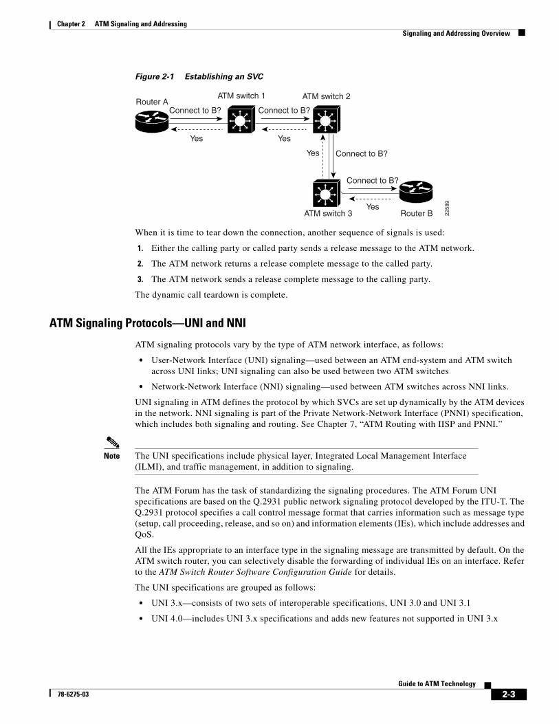
Connection Setup and Signaling
Figure 2-1 demonstrates how a basic SVC is set up from Router A (the calling party) to Router B (the called party) using signaling. The steps in the process are as follows:
1. Router A sends a signaling request packet to its directly connected ATM switch (ATM switch 1).
This request contains the ATM address of both calling and called parties, as well as the basic traffic contract requested for the connection.
2. ATM switch 1 reassembles the signaling packet from Router A and then examines it.
3. If ATM switch 1 has an entry for Router B’s ATM address in its switch table, and it can accommodate the QoS requested for the connection, it reserves resources for the virtual connection and forwards the request to the next switch (ATM switch 2) along the path.
4. Every switch along the path to Router B reassembles and examines the signaling packet, then forwards it to the next switch if the traffic parameters can be supported on the ingress and egress interfaces. Each switch also sets up the virtual connection as the signaling packet is forwarded.
If any switch along the path cannot accommodate the requested traffic contract, the request is rejected and a rejection message is sent back to Router A.
5. When the signaling packet arrives at Router B, Router B reassembles it and evaluates the packet. If Router B can support the requested traffic contract, it responds with an accept message. As the accept message is propagated back to Router A, the virtual connection is completed.
Note Because the connection is set up along the path of the connection request, the data also flows along this same path.
2-2Guide to ATM Technology
78-6275-03
Chapter 2 ATM Signaling and AddressingSignaling and Addressing Overview
Figure 2-1 Establishing an SVC
When it is time to tear down the connection, another sequence of signals is used:
1. Either the calling party or called party sends a release message to the ATM network.
2. The ATM network returns a release complete message to the called party.
3. The ATM network sends a release complete message to the calling party.
The dynamic call teardown is complete.
ATM Signaling Protocols—UNI and NNI
ATM signaling protocols vary by the type of ATM network interface, as follows:
• User-Network Interface (UNI) signaling—used between an ATM end-system and ATM switch across UNI links; UNI signaling can also be used between two ATM switches
• Network-Network Interface (NNI) signaling—used between ATM switches across NNI links.
UNI signaling in ATM defines the protocol by which SVCs are set up dynamically by the ATM devices in the network. NNI signaling is part of the Private Network-Network Interface (PNNI) specification, which includes both signaling and routing. See Chapter 7, “ATM Routing with IISP and PNNI.”
Note The UNI specifications include physical layer, Integrated Local Management Interface (ILMI), and traffic management, in addition to signaling.
The ATM Forum has the task of standardizing the signaling procedures. The ATM Forum UNI specifications are based on the Q.2931 public network signaling protocol developed by the ITU-T. The Q.2931 protocol specifies a call control message format that carries information such as message type (setup, call proceeding, release, and so on) and information elements (IEs), which include addresses and QoS.
All the IEs appropriate to an interface type in the signaling message are transmitted by default. On the ATM switch router, you can selectively disable the forwarding of individual IEs on an interface. Refer to the ATM Switch Router Software Configuration Guide for details.
The UNI specifications are grouped as follows:
• UNI 3.x—consists of two sets of interoperable specifications, UNI 3.0 and UNI 3.1
• UNI 4.0—includes UNI 3.x specifications and adds new features not supported in UNI 3.x
ATM switch 1Router A
Router B
ATM switch 2
ATM switch 3
Connect to B? Connect to B?
Yes Yes
Yes Connect to B?
Connect to B?
Yes
2258
9
2-3Guide to ATM Technology
78-6275-03

Chapter 2 ATM Signaling and AddressingSignaling and Addressing Overview
The original UNI signaling specification, UNI 3.0, provided for the following features:
• Signaling for point-to-point connections and point-to-multipoint connections
• Support for bandwidth symmetric and bandwidth asymmetric traffic
UNI 3.1 includes the provisions of UNI 3.0 but provides for a number of changes, a number of which were intended to bring the earlier specifications into conformance with ITU-T standards.
UNI 4.0 replaced an explicit specification of the signaling protocol with a set of deltas between it and ITU-T signaling specifications. In general, the functions in UNI 4.0 are a superset of UNI 3.1, and include both a mandatory core of functions and many optional features.
• Anycast signaling—allows connection requests and address registration for group addresses, where the group address can be shared among multiple end systems; the group address can represent a particular service, such as a configuration or name server.
• Explicit signaling of QoS parameters—maximum cell transfer delay (MCTD), peak-to-peak cell delay variation (ppCDV), and cell loss ratio (CLR) can be signaled across the UNI for CBR and VBR SVCs.
• Signaling for ABR connections—many parameters can be signaled to create ABR connections.
• Virtual UNI—provides for using one physical UNI with multiple signaling channels. For example, several end stations can connect through a multiplexor; the multiplexor connects via UNI to an ATM switch. In this case there are multiple signaling channels being used by the end stations, but only one UNI (the virtual UNI).
• PNNI—specifies signaling and routing protocols across the NNI. PNNI is an optional addition to the UNI 4.0; for detailed information see Chapter 7, “ATM Routing with IISP and PNNI.”
The following optional features in UNI 4.0 are not supported on the ATM switch router:
• Proxy signaling—allows a device, called a proxy signaling agent, to signal on behalf of other devices. For example, a router might signal for devices behind it that do not support signaling. Another use for proxy signaling would be a video server with aggregated links (say, three 155 Mbps links aggregated for the 400 Mbps required by video); in this case, where there is really just one connection, one of the links would signal on behalf of all three.
• Signaling for point-to-multipoint connections—leaf initiated joins are supported.
Note Your ATM switch router supports UNI 3.0, 3.1, and 4.0.
AddressingATM addresses are needed for purposes of signaling when setting up switched connections. ATM addresses are also used by the Integrated Local Management Protocol (ILMI, formerly Interim Local Management Protocol) to learn the addresses of neighboring switches.
ATM Address Formats
The ITU-T long ago settled on telephone number-like addresses, called E.164 addresses or E.164 numbers, for use in public ATM (B-ISDN) networks. Since telephone numbers are a public (and expensive) resource, the ATM Forum set about developing a private network addressing scheme. The ATM Forum considered two models for private ATM addresses: a peer model, which treats the ATM layer as a peer of existing network layers, and a subnetwork, or overlay, model, which decouples the ATM layer from any existing protocol and defines for itself an entirely new addressing structure.
2-4Guide to ATM Technology
78-6275-03

Chapter 2 ATM Signaling and AddressingSignaling and Addressing Overview
The ATM Forum settled on the overlay model and defined an ATM address format based on the semantics of an OSI Network Service Access Point (NSAP) address. This 20-byte private ATM address is called an ATM End System Address (AESA), or ATM NSAP address (though it is technically not a real NSAP address). It is specifically designed for use with private ATM networks, while public networks typically continue to use E.164 addresses.
The general structure of NSAP format ATM addresses, shown in Figure 2-2, is as follows:
• An initial domain part (IDP)—consists of two elements: an authority and format identifier (AFI) that identifies the type and format of the second element, the initial domain identifier (IDI). The IDI identifies the address allocation and administration authority.
• A domain specific part (DSP)—contains the actual routing information in three elements: a high-order domain specific part (HO-DSP), an end system identifier (ESI), which is the MAC address, and NSAP selector (SEL) field, used to identify LAN emulation (LANE) components.
Figure 2-2 Private ATM Network Address Formats
AFI SELDCC
IDP
IDI
ESIHO-DSP
20 Bytes
DCC ATM format
AFI SELICD
IDP
IDI
ESI
ICD ATM format
NSAP format E.164
AFI SEL
IDP
IDI
ESIHO-DSP
HO-DSP
HO-DSPE.164
ICDDSPIDPESI
AFIDCCIDI
= International Code Designator= Domain Specific Part= Initial Domain Part= End System Identifier (MAC address)
= Authority and Format Identifier= Data Country Code= Initial Domain Identifier
2259
2
2-5Guide to ATM Technology
78-6275-03

Chapter 2 ATM Signaling and AddressingAddressing on the ATM Switch Router
Private ATM address formats are of three types that differ by the nature of their AFI and IDI (see Figure 2-2):
• DCC format (AFI=39)—the IDI is a Data Country Code (DCC). DCC addresses are administered by the ISO national member body in each country.
• ICD format (AFI=47)—the IDI is an International Code Designator (ICD). ICD address codes identify particular international organizations and are allocated by the British Standards Institute.
• NSAP encoded E.164 format (AFI=45)—the IDI is an E.164 number.
Note There are two types of E.164 addresses: the NSAP encoded E.164 format and the E.164 native format, sometimes called an E.164 number, used in public networks.
A sample ATM address, 47.00918100000000E04FACB401.00E04FACB401.00, is shown in Figure 2-3. The AFI of 47 identifies this address as a ICD format address.
Figure 2-3 Example of ICD Format Address
Choosing an Address Format
The ATM Forum specifications through UNI 4.0 only specify these three valid types of AFI. However, future ATM Forum specifications will allow any AFI that has binary encoding of the Domain Specific Part (DSP) and a length of 20 octets. Although your Cisco ATM switch router ships with an autoconfigured NSAP format ATM address of the ICD type, similar to the one shown in Figure 2-3, the ATM switch router does not restrict the AFI values; you can use any of the valid formats.
The ATM Forum recommends that organizations or private network service providers use either the DCC or ICD formats to form their own numbering plan. NSAP encoded E.164 format addresses are used for encoding E.164 numbers within private networks that need to connect to public networks that use native E.164 addresses, but they can also be used by some private networks. Such private networks can base their own (NSAP format) addressing on the E.164 address of the public UNI to which they are connected and take the address prefix from the E.164 number, identifying local nodes by the lower order bits. The use of E.164 addresses is further discussed in the “Signaling and E.164 Addresses” section on page 2-11.
Addressing on the ATM Switch RouterThe ATM address is used by the ATM switch router for signaling and management functions, and by protocols such as LAN emulation and PNNI. The ATM switch router ships with a preconfigured default address which allows it to function in a plug-and-play manner. You can change the default address if you need to; the main reasons for doing so are listed in the section “Manually Configured ATM Addresses” section on page 2-10. If you do not foresee needing to reconfigure the ATM address, then the details of the following sections might not concern you.
AFI ICD HO-DSP ESI SEL
47 0091 8100000000E04FACB401 00E04FACB401 00
2259
3
2-6Guide to ATM Technology
78-6275-03

Chapter 2 ATM Signaling and AddressingAddressing on the ATM Switch Router
Autoconfigured ATM Addressing SchemeDuring initial startup, the ATM switch router generates an ATM address using the following defaults (see Figure 2-4):
• AFI=47—indicates an address of type DCC
• ICD=0091(Cisco-specific)
• Cisco-specific address type (part of HO-DSP)=81000000
• Cisco switch ID=MAC format address
• ESI=MAC address repeated
Note The MAC address used in the Cisco switch ID and ESI fields is the default MAC address for the ATM switch router. It might not be the same as the address printed on the chassis label.
• Selector equals 0—1 byte
Figure 2-4 ATM Address Default Format
The autoconfigured address mechanism provides a default ATM address for the unconfigured switch. This default address is used by the following protocols:
• The Integrated Local Management Interface (ILMI)—a protocol and part of the UNI specifications that facilitates sharing of management information across the UNI. ILMI uses the first 13 bytes of this address to hand to end systems for the generation of ESI addresses. See the “ILMI Use of the ATM Address” section on page 2-9.
• Private Network-Network Interface (PNNI)—a dynamic routing protocol for ATM networks. PNNI uses the 13-byte prefix to establish itself as a node in a single-level PNNI routing domain and the first 7 bytes to construct the default peer group identifier. For a complete discussion, see Chapter 7, “ATM Routing with IISP and PNNI.”
CiscoICD
Address type(reserved)
Cisco switchID
47 81 00 00 00 MAC Address
2 bytes 3 bytes
Default PNNIpeer-group ID
Default ILMI address registration prefixand default PNNI summary address prefix
6 bytes 6 bytes
H59
04
1 byte
MAC Address 00
ESIAFI SEL
1 byte
1 byte
00 91
2-7Guide to ATM Technology
78-6275-03

Chapter 2 ATM Signaling and AddressingAddressing on the ATM Switch Router
Default Address Format Features and Implications
Using the default address format has the following features and implications:
• All preconfigured addresses share the same 7-byte address prefix. In the autoconfigured address for a given ATM switch router, the same MAC address is used for bytes 8 through 13 and bytes 14 through 19.
• The default autoconfigured address provides plug-and-play operation. You can reconfigure the ATM address using your own addressing style, but you must use a globally unique MAC address to generate the ATM address.
• The autoconfigured addressing scheme suffices for PNNI operation in a single-level routing domain. To achieve scalable ATM routing in large ATM networks with multiple levels of PNNI hierarchy, you need to manually configure ATM addresses.
The example display below shows the autoconfigured ATM addresses on the ATM switch router. Note that the 13-byte ILMI switch prefix is the same for all addresses.
Switch# show atm addresses
Switch Address(es): 47.00918100000000E04FACB401.00E04FACB401.00 active
Soft VC Address(es): 47.0091.8100.0000.00e0.4fac.b401.4000.0c80.1000.00 ATM0/1/0 47.0091.8100.0000.00e0.4fac.b401.4000.0c80.1010.00 ATM0/1/1 47.0091.8100.0000.00e0.4fac.b401.4000.0c80.1020.00 ATM0/1/2 47.0091.8100.0000.00e0.4fac.b401.4000.0c80.1030.00 ATM0/1/3 47.0091.8100.0000.00e0.4fac.b401.4000.0c80.8000.00 ATM1/0/0 47.0091.8100.0000.00e0.4fac.b401.4000.0c80.8010.00 ATM1/0/1 47.0091.8100.0000.00e0.4fac.b401.4000.0c80.8020.00 ATM1/0/2 47.0091.8100.0000.00e0.4fac.b401.4000.0c80.8030.00 ATM1/0/3 47.0091.8100.0000.00e0.4fac.b401.4000.0c80.9000.00 ATM1/1/0 47.0091.8100.0000.00e0.4fac.b401.4000.0c80.9010.00 ATM1/1/1 47.0091.8100.0000.00e0.4fac.b401.4000.0c80.9020.00 ATM1/1/2 47.0091.8100.0000.00e0.4fac.b401.4000.0c80.9030.00 ATM1/1/3 47.0091.8100.0000.00e0.4fac.b401.4000.0c81.8030.00 ATM-P3/0/3 47.0091.8100.0000.00e0.4fac.b401.4000.0c81.9000.00 ATM3/1/0 47.0091.8100.0000.00e0.4fac.b401.4000.0c81.9010.00 ATM3/1/1 47.0091.8100.0000.00e0.4fac.b401.4000.0c81.9020.00 ATM3/1/2 47.0091.8100.0000.00e0.4fac.b401.4000.0c81.9030.00 ATM3/1/3 47.0091.8100.0000.00e0.4fac.b401.4000.0c82.0000.00 ATM-P4/0/0
Soft VC Address(es) for Frame Relay Interfaces : 47.0091.8100.0000.00e0.4fac.b401.4000.0c82.0010.00 Serial4/0/0:1 47.0091.8100.0000.00e0.4fac.b401.4000.0c82.0020.00 Serial4/0/0:2 47.0091.8100.0000.00e0.4fac.b401.4000.0c82.0030.00 Serial4/0/0:3 47.0091.8100.0000.00e0.4fac.b401.4000.0c82.0210.00 Serial4/0/1:1 47.0091.8100.0000.00e0.4fac.b401.4000.0c82.0220.00 Serial4/0/1:2
ILMI Switch Prefix(es): 47.0091.8100.0000.00e0.4fac.b401
ILMI Configured Interface Prefix(es):
LECS Address(es): 47.0091.8100.0000.00e0.4fac.b401.0010.0daa.cc43.00
2-8Guide to ATM Technology
78-6275-03

Chapter 2 ATM Signaling and AddressingAddressing on the ATM Switch Router
ILMI Use of the ATM AddressILMI reduces the need for manual configuration of attached end systems and is important in the operation of ATM networks. One of its most useful features, address registration, greatly facilitates the administration of ATM addresses.
The ILMI address registration mechanism allows an ATM end system to inform an ATM switch of its unique MAC address and to receive the remainder of the node's full ATM address in return. ILMI uses the first 13 bytes of the ATM address as the switch prefix that it registers with end systems.
When the an end system, such as a router (Figure 2-5), is attached to the ATM switch, ILMI is used to send all the router’s MAC addresses (ESIs) to the switch. The ESI is appended to the switch’s 13-byte ILMI prefix to make up a complete ATM address, which is then associated with the interface on which it received the ESI. This allows the ATM switch router, upon receiving a call setup request, to know which interface to send on.
Figure 2-5 ILMI Address Registration Across the UNI
ILMI Considerations for ATM Address Migration
During address migration (changing from one addressing scheme to another), multiple addresses can be configured for a single switch. ILMI registers end systems with multiple prefixes during this period until an old address is removed. (PNNI automatically summarizes all of the switch’s prefixes in its reachable address advertisement.)
Although the default, autoconfigured address provides for a fixed 13-byte ILMI prefix, the ATM switch router allows configuration of per-interface ILMI address prefixes, so that different address prefixes can be registered with end systems attached to different interfaces. When any per-interface ILMI address prefixes are configured, they override the prefix(es) derived from the first 13 bytes of the switch ATM address(es) for that specific interface.
ILMI access filters can provide security by permitting or denying ILMI registration of different classes of addresses. For details, see the ATM Switch Router Software Configuration Guide.
Additional ILMI Functions
The ILMI protocol uses SNMP format packets across the UNI to access an ILMI Management Information Base (MIB) associated with the link, within each node. The ILMI protocol facilitates network-wide autoconfiguration by allowing adjacent nodes to determine various characteristics of each other—for example, the size of each other's connection space, the type of signaling used (UNI, NNI), type of link (public, private), hooks for network management autodiscovery, and so on. The ATM routing protocols, PNNI and IISP, use this information to automatically discover and bring up a network of interconnected ATM switch routers.
UNI
ILMI protocol
ESI
Address prefix
2259
4
2-9Guide to ATM Technology
78-6275-03
Chapter 2 ATM Signaling and AddressingAddressing on the ATM Switch Router
ILMI is also used to inform LANE clients of the location of the LANE configuration server (LECS). ILMI on the ATM switch router also allows the switch to provide Cisco ATM adapters with the address of an ATM Address Resolution Protocol (ATMARP) server, which in turn allows plug-and-play operation of ATM desktops.
PNNI Use of the ATM AddressThe preconfigured address provides plug-and-play operation in isolated flat topology ATM networks. All switches with autoconfigured ATM addresses will form one peer group. Although the preconfigured addresses are globally unique, they are not suitable for connection to service provider networks or within hierarchical PNNI networks. Furthermore, address summarization, a key feature of hierarchical PNNI, is not possible beyond the level of one ATM switch. In addition, while E.164 numbers are supported on UNI and IISP interfaces, they are not directly supported by PNNI. Instead, these are supported indirectly through use of the E.164 AESA format.
See Chapter 7, “ATM Routing with IISP and PNNI” for more information about addressing in hierarchical PNNI networks and about using E.164 AESAs with PNNI.
LAN Emulation Use of the ATM AddressOn a LAN, packets are addressed by the MAC-layer address of the destination and source stations. To provide similar functionality, LAN emulation (LANE) must support some form of MAC-to-ATM address mapping. All LANE client and server components must therefore have a unique ATM address.
The ATM switch router provides a means of automatically assigning ATM addresses for LANE components. See the “Addressing” section on page 6-10.
Manually Configured ATM AddressesThe following situations require manually configuring the ATM address:
• To connect to another system using IISP. Using IISP means that PNNI must be disabled, so there is no ILMI support. In this case the ATM address must be manually configured. For further details, see Chapter 7, “ATM Routing with IISP and PNNI.”
• To configure a new ATM address that replaces the previous ATM address and generates a new PNNI node ID and peer group ID for migrating from flat to hierarchical PNNI.
• To connect to multiple levels of a PNNI hierarchy.
• To connect to a service provider network that requires you to use their addressing scheme.
• To use a particular style of addressing. For instance, in some circumstances a mnemonic scheme might be useful for identifying nodes in an ATM network.
For instructions on manually configuring the ATM address, refer to the ATM Switch Router Software Configuration Guide. See the “Obtaining Registered ATM Addresses” section on page 2-17 in this guide for information about registered ATM addresses.
Caution ATM addressing can lead to conflicts if not configured correctly. The correct address must always be present. For instance, if you are configuring a new ATM address, the old one must be completely removed from the configuration. Also, it is important to maintain the uniqueness of the address across large networks.
2-10Guide to ATM Technology
78-6275-03

Chapter 2 ATM Signaling and AddressingSignaling and E.164 Addresses
Signaling and E.164 AddressesThe NSAP-encoded E.164 ATM address format includes an embedded E.164 address (see Figure 2-2), the form of address generally used in telephone networks. Private networks can use this address format by taking an assigned E.164 address from a service provider and using the ESI part of the ATM address space to identify local nodes. The ATM switch router also includes support for E.164 translation, which allows networks that use private ATM addresses (DCC, ICD, or NSAP-encoded E.164) to work with networks that use E.164 native addresses. E.164 native addresses are used in many public TDM networks and in ATM-attached PBX devices.
E.164 numbers, or native E.164 addresses, are in ASCII format and conform to ITU E.164 specifications. They have the following properties:
• Contain 7 to 15 digits, integers 0 through 9
• Result equals one digit per byte; for example, 1–800–555–1212 is 3138303035353531323132
These properties are carried in the called and calling party address IEs, which are part of the signaling packets used to set up a call. Native E.164 addresses are supported on UNI and Interim Interswitch Signaling Protocol (IISP) interfaces. PNNI does not support E.164 addresses directly, but uses the NSAP encoded (embedded) E.164 format. For information on using E.164 addresses with PNNI, see Chapter 7, “ATM Routing with IISP and PNNI.”
Embedded E.164 addresses are of two types:
• E164_AESA—An AESA address with an embedded E.164 number; for example, 45.000007654321111FDDDDDDDD.CCCCCCCCCCCC.00. The “D” and “C” characters in this example represent an end system address.
• E164_ZDSP—An AESA address with all zeros after the embedded E.164 number; for example, 45.000001234567777F00000000.000000000000.00. ZDSP means “zero domain specific part.”
When a call traverses a public ATM network with E.164 native addresses, the addresses must be translated between the private and public formats. In Figure 2-6, a call from private network A must traverse the public ATM network to reach private network B. When the call leaves the egress switch of the private network, the NSAP source and destination addresses are translated into E.164 format, while preserving the NSAP source and destination addresses, carried in the IE part of the signaling packet. At the ingress switch, the address is translated back into the NSAP format used on private network B.
Figure 2-6 Address Remapping Across a Public ATM Network
Privatenetwork A
Privatenetwork B
PublicATM network
NSAP-A NSAP-B
E.164-A E.164-B
Ingress switch
SOURCE=E.164-ASOURCESUB=NSAP-A
DEST=E.164-BDESTSUB=NSAP-B
DEST=NSAP-BSOURCE=NSAP-A
2259
5
2-11Guide to ATM Technology
78-6275-03

Chapter 2 ATM Signaling and AddressingSignaling and E.164 Addresses
E.164 Address Conversion OptionsThe ATM switch router provides three options for performing the address translation needed between private and public addresses. The feature you choose depends on the address format you are using on your ATM network. The features are as follows:
• E.164 gateway—Use this feature when addresses are in ICD or DCC format and a call must traverse an E.164 network.
• E.164 address autoconversion—Use this feature when addresses are in E164_ZDSP or E.164_AESA format and a call must traverse an E.164 network.
• E.164 address one-to-one translation table—Use this feature to create an E.164 to NSAP address translation table manually. This feature is not recommended for most networks.
The E.164 Gateway Feature
The E.164 gateway feature allows calls with AESAs to be forwarded, based on prefix matching, on interfaces that are statically mapped to E.164 addresses. To configure the E.164 gateway feature, you first configure a static ATM route with an E.164 address, then configure the E.164 address to use on the interface. When a static route is configured on an interface, all ATM addresses that match the configured address prefix are routed through that interface to an E.164 address.
Figure 2-7 illustrates how the E.164 gateway feature works. The AESA address is used to initiate the call at the ingress to the public network. The public network routes the call based on the E.164 address. Signaling uses the E.164 address in the called and calling part IEs, and uses AESA addresses in the called and calling part subaddress IEs. The AESA address is used to complete the call at the egress from the public network.
Figure 2-7 E.164 Gateway Conversion Example
When the E.164 gateway feature is configured, the ATM switch router first attempts to make a connection using the E.164 gateway feature. If that connection fails, the switch attempts to make the connection using the E.164 address autoconversion feature, as described in the following section.
E.164public
network
1422
4
Switch A Switch B
Originates as:Calling AESA: 47.11111…Calling subaddress: NoneCalled AESA: 47.22222…Called subaddress: None
E.164 address: 1234567
Signaled as:Calling E.164: 31323334353637Calling subaddress: 47.11111…Called E.164: 37363534333231Called subaddress: 47.22222…
E.164 address: 7654321
Converted back to:Calling AESA: 47.11111…Calling subaddress: NoneCalled AESA: 47.22222…Called subaddress: None
0/0/0
End system A
0/0/1
End system B
2-12Guide to ATM Technology
78-6275-03

Chapter 2 ATM Signaling and AddressingSignaling and E.164 Addresses
Configuration Overview
Configuring the E.164 gateway feature requires the following steps:
Step 1 Configure a static route with a 13-byte ATM address prefix on an interface with an E.164 address.
Step 2 Enter interface configuration mode for outgoing interface and assign the E.164 address to the interface.
The E.164 Address Autoconversion Feature
The E.164 address autoconversion feature uses the embedded E.164 number in the E164_ZDSP or E164_AESA address to perform the address conversion. To configure this feature, you set up a static route prefix with the E.164 address, then enable the E.164 autoconversion feature.
The E.164 portion of an E.164 ATM address is the first 15 digits following the authority and format identifier (AFI) of 45, shown in Figure 2-8. The E.164 portion is right justified and ends with an “F.” If all fifteen digits are not being used, the unused digits are filled with zeros. In Figure 2-8, the embedded E.164 number is 1234567777, but it is signaled at the egress of the switch and in the E.164 public network as 31323334353637373737.
Figure 2-8 E.164 Portion of an E.164 ATM Address
The autoconversion process differs slightly between the E164_ZDSP and E164_AESA address formats. Table 2-1 compares the E.164 address autoconversion process by address type. The main difference between the two types is the way the IEs are signaled at the egress of the switch, as described in the second row of Table 2-1.
Note During the final conversion process, the calling AESA and called AESA return to their original values.
45.000001234567777F00000000.000000000000.00
S68
87E.164 portion
2-13Guide to ATM Technology
78-6275-03

Chapter 2 ATM Signaling and AddressingSignaling and E.164 Addresses
Figure 2-9 shows an example of an E164_ZDSP address autoconversion. In Figure 2-9, a call (connection) from end system A is placed to end system B on the other side of an E.164 public network. The call originates as an E.164 ATM address and is signaled in native E.164 format at the egress port of switch A and within the E.164 public network. When the call reaches the ingress port of switch B, at the edge of the E.164 public network, the call is converted back to E.164 ATM address format.
Note The ATM switch router routes calls based on the E.164 ATM address (not the native E.164 address).
Table 2-1 E164_ZDSP and E164_AESA Address Autoconversion Comparison
Action E164_ZDSP E164_AESA
Originates as
Calling AESA: 45.000001234567777F00000000.000000000000.00
Calling subaddress: None
Called AESA: 45.000007654321111F00000000.000000000000.00
Called subaddress: None
Calling AESA: 45.000001234567777FAAAAAAAA.BBBBBBBBBBBB.00
Calling subaddress: None
Called AESA: 45.000007654321111FCCCCCCCC.DDDDDDDDDDDD.00
Called subaddress: None
Signaled at egress of switch as
Calling E.164: 31323334353637373737
Calling subaddress: None
Called E.164: 37363534333231313131
Called subaddress: None
Calling E.164: 31323334353637373737
Calling subaddress: 45.0000012345677777FAAAAAAAA.BBBBBBBBBBBB.00
Called E.164: 37363534333231313131
Called subaddress: 45.000007654321111FCCCCCCCC.DDDDDDDDDDDD.00
Converted back at ingress of switch to
Calling AESA: 45.000001234567777F00000000.000000000000.00
Calling subaddress: None
Called AESA: 45.000007654321111F00000000.000000000000.00
Called subaddress: None
Calling AESA: 45.000001234567777FAAAAAAAA.BBBBBBBBBBBB.00
Calling subaddress: None
Called AESA: 45.000007654321111FCCCCCCCC.DDDDDDDDDDDD.00
Called subaddress: None
2-14Guide to ATM Technology
78-6275-03

Chapter 2 ATM Signaling and AddressingSignaling and E.164 Addresses
Figure 2-9 E164_ZDSP Address Autoconversion Example
Figure 2-10 shows an example of an E164_AESA address autoconversion. In Figure 2-10, a call from end system A is placed to end system B on the other side of an E.164 public network. The call originates as an E.164 ATM address at the egress port of switch A and within the E.164 public network:
• The E.164 ATM address is signaled in native E.164 format.
• The called party address (45.000007654321111F...) IE is put in the called party subaddress IE.
• The calling party address (45.000001234567777F...) IE is put in the calling party subaddress IE.
When the call reaches the ingress port of switch B, at the edge of the E.164 public network, the call is converted back to E.164 ATM address format and the following events occur:
• The native E.164 address is converted back to an E.164 ATM address.
• The called party subaddress (45.000007654321111F...) IE is returned to the called party address IE.
• The calling party subaddress (45.000001234567777F...) IE is returned to the calling party address IE.
E.164public
network
1422
5
Switch A Switch B
Originates as:Calling AESA: 45.000001234567777F0…Calling subaddress: NoneCalled AESA: 45.000007654321111F0…Called subaddress: None
Signaled as:Calling E.164: 31323334353637373737Calling subaddress: NoneCalled E.164: 37363534333231313131Called subaddress: None
Converted back to:Calling AESA: 45.000001234567777F0…Calling subaddress: NoneCalled AESA: 45.000007654321111F0…Called subaddress: None
End system A
End system B
2-15Guide to ATM Technology
78-6275-03
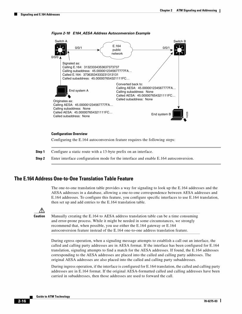
Chapter 2 ATM Signaling and AddressingSignaling and E.164 Addresses
Figure 2-10 E164_AESA Address Autoconversion Example
Configuration Overview
Configuring the E.164 autoconversion feature requires the following steps:
Step 1 Configure a static route with a 13-byte prefix on an interface.
Step 2 Enter interface configuration mode for the interface and enable E.164 autoconversion.
The E.164 Address One-to-One Translation Table Feature
The one-to-one translation table provides a way for signaling to look up the E.164 addresses and the AESA addresses in a database, allowing a one-to-one correspondence between AESA addresses and E.164 addresses. To configure this feature, you configure specific interfaces to use E.164 translation, then set up and add entries to the E.164 translation table.
Caution Manually creating the E.164 to AESA address translation table can be a time consuming and error-prone process. While it might be needed in some circumstances, we strongly recommend that, when possible, you use either the E.164 gateway or E.164 autoconversion feature instead of the E.164 one-to-one address translation feature.
During egress operation, when a signaling message attempts to establish a call out an interface, the called and calling party addresses are in AESA format. If the interface has been configured for E.164 translation, signaling attempts to find a match for the AESA addresses. If found, the E.164 addresses corresponding to the AESA addresses are placed into the called and calling party addresses. The original AESA addresses are also placed into the called and calling party subaddresses.
During ingress operation, if the interface is configured for E.164 translation, the called and calling party addresses are in E.164 format. If the original AESA-formatted called and calling addresses have been carried in subaddresses, then those addresses are used to forward the call.
E.164public
network
1422
6
Switch A Switch B
Originates as:Calling AESA: 45.000001234567777FA…Calling subaddress: NoneCalled AESA: 45.000007654321111FC…Called subaddress: None
Signaled as:Calling E.164: 31323334353637373737Calling subaddress: 45.0000012345677777FA…Called E.164: 37363534333231313131Called subaddress: 45.000007654321111FC…
Converted back to:Calling AESA: 45.000001234567777FA…Calling subaddress: NoneCalled AESA: 45.000007654321111FC…Called subaddress: None
0/0/0
End system A
0/0/1 0/0/1
End system B
2-16Guide to ATM Technology
78-6275-03

Chapter 2 ATM Signaling and AddressingObtaining Registered ATM Addresses
If subaddresses are not present because the network blocks them, or because the switch at the entry to the E.164 network does not use subaddresses, signaling attempts to find a match for the AESA address in the ATM E.164 translation table.
If matches are found, the AESA addresses corresponding to the E.164 addresses in the translation table are placed into the called and calling party addresses. The call is then forwarded using the AESA addresses.
Configuration Overview
Configuring the E.164 address one-to-one translation feature requires the following tasks:
Step 1 Select the interface to configure and enter interface configuration mode.
Step 2 Enable E.164 translation.
Step 3 Enter E.164 translation table configuration mode.
Step 4 Add the entries to the translation table. Each entry contains an E.164 address and corresponding NSAP address.
Obtaining Registered ATM AddressesTo satisfy the uniqueness requirement and facilitate distribution, a number of registration authorities administer ATM addresses. These addresses are usually distributed in sets of addresses having a common prefix. The uniqueness of the prefix, which is used to define a group of addresses, is ensured by the registration authority. The recipient then allocates the remaining part of the ATM address using an addressing scheme that is appropriate for the private network to create a set of unique addresses. If these guidelines are followed, private ATM networks can achieve global ATM interconnection without the need to renumber addresses. At the end of this section are some references that contain information on how to obtain a globally unique ATM prefix.
AESA prefixes are differentiated by ownership, as follows:
• Customer-owned ATM prefix—a prefix allocated directly to a private network by a national or world registration authority.
• Service provider ATM prefix—a prefix allocated to a service provider by a national or world registration authority. An ATM service provider might suballocate part of its address space to its customers.
• Unregistered ATM prefix—a prefix, or an extension of such a prefix, that is not obtained from a national or world registration authority. Private ATM networks can use unregistered prefixes to derive unregistered addresses, but these addresses are only used within that private network because they are not guaranteed to be globally unique.
If you have a private network, you can obtain ATM prefixes from the following:
• An ATM service provider. Any AESA format is acceptable.
• The national registration authority. In the USA, the national registration authority is American National Standards Institute (ANSI). In the United Kingdom, the national registration authority is the Federation of the Electronics Industry (FEI).
A customer owned ATM address (assigned by Cisco) is preconfigured on every ATM switch router. If you are not implementing hierarchy in your PNNI network and do not plan to interconnect to a global ATM internetwork, you can use the preconfigured ATM address.
2-17Guide to ATM Technology
78-6275-03

Chapter 2 ATM Signaling and AddressingSpecial Signaling Features
ATM service providers can obtain the following types of ATM addresses:
• E.164 numbers or E.164 AESAs from the ITU or the national numbering authority.
• ICD AESAs from the British Standards Institute (BSI) by way of a national registration authority.
• DCC AESAs from the national registration authority. In the USA, the national registration authority is ANSI. In the United Kingdom, the national registration authority is FEI.
A good source for an ICD ATM prefix is the IOTA scheme administered by BSI. It is preferable to US DCC AESAs. The documentation on how to get an organizational identifier and how to construct a AESA from the organizational identifier is also easier to follow for IOTA than that for US DCC AESAs. For more information, see http://www.bsi.org.uk/disc/iota.html.
The following additional publications can also provide guidance on how to obtain a globally unique ATM prefix:
• “ATM Forum Addressing User Guide,” STR-RA-ADDR-USER-001.02, Straw Ballot, October, 1998.
• “ATM Forum Addressing Reference Guide,” STR-RA-ADDR-01.08, Straw Ballot, October, 1998.
Special Signaling FeaturesThere are several special-purpose signaling features that can be configured on the ATM switch router. The following subsections provide discussions of the following features:
• Closed user group signaling
• Multipoint-to-point funnel signaling
The following additional signaling features are described in the ATM Switch Router Software Configuration Guide:
• Signaling IE forwarding
• ATM SVC frame discard
• Signaling diagnostics tables
• Disabling signaling on an interface
Closed User Group SignalingThe signaling capabilities of the ATM switch router allow you to define closed user groups (CUGs), which function as ATM virtual private networks (VPNs).
Multiple CUGs can be defined, and a specific user can be a member of one or more CUGs. Members of a CUG can communicate among themselves, but not with users outside the group. Specific users can have additional restrictions that prevent them from originating or receiving calls from other members of the CUG. You can also specify additional restrictions on originating and receiving calls to or from members of other CUGs.
For example, if you have three CUGs (A, B, and C) in your network, you can configure them so that groups B and C can communicate with group A without restriction, but groups B and C cannot communicate between each other.You can also configure specific members of the same group to not accept calls from members of the same group.
2-18Guide to ATM Technology
78-6275-03

Chapter 2 ATM Signaling and AddressingSpecial Signaling Features
The basis for CUGs are interlock codes. Interlock codes are unique in the whole network. Members belonging to a CUG are assigned a unique interlock code. Members of CUGs use this interlock code while communicating with other members of the same or different CUGs.
The interlock code is passed in CUG interlock code information element (CUG IC IE). The CUG IE also carries information that specifies whether the call can go through if the called party is not a member of the specified CUG. At the network boundary where the call originates, when a call is received from the user, the ATM switch router generates the CUG IE and sends it as part of the SETUP message. In this software release, the CUG IE can only contain the preferential CUG's interlock code. The CUG IE is used at the destination network interface to determine if the call should be forwarded or rejected. The CUG IE is forwarded transparently by the intermediate switches.
Note End systems do not have any knowledge of interlock codes.
In general, two types of interlock codes are defined:
• Global interlock code is 24 bytes long and consists of a globally unique AESA format address used to identify the network administering the CUG, followed by a 4-byte suffix assigned to this CUG by the network administration.
• International interlock code is 4 bytes long and consists of 4 binary coded decimal (BCD) digits containing a country code and network code, followed by a 2-byte suffix assigned to this CUG by the network administration.
Note Your Cisco ATM switch router supports only the 24-byte interlock code.
Figure 2-11 provides examples of CUGs with the following characteristics:
• U1, U2, and U4 are members of CUG I.
• U3 and U6 are members of CUG J.
• U6, U7, U8, U9, and U10 are members of CUG K.
• U5, U11, and U12 do not belong to any closed user groups.
• U6 belongs to both CUG J and CUG K.
2-19Guide to ATM Technology
78-6275-03
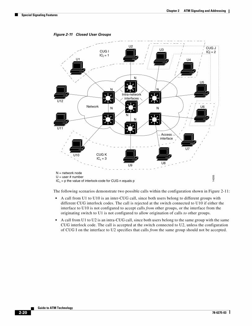
Chapter 2 ATM Signaling and AddressingSpecial Signaling Features
Figure 2-11 Closed User Groups
The following scenarios demonstrate two possible calls within the configuration shown in Figure 2-11:
• A call from U1 to U10 is an inter-CUG call, since both users belong to different groups with different CUG interlock codes. The call is rejected at the switch connected to U10 if either the interface to U10 is not configured to accept calls from other groups, or the interface from the originating switch to U1 is not configured to allow origination of calls to other groups.
• A call from U1 to U2 is an intra-CUG call, since both users belong to the same group with the same CUG interlock code. The call is accepted at the switch connected to U2, unless the configuration of CUG I on the interface to U2 specifies that calls from the same group should not be accepted.
Intra-networkinterfaces
Network
N
N
N
N
NN
N
U1
U2U3
U4
U5
U6
U7
U8U9
U10
U11
CUG KICk = 3
CUG JICj = 2CUG I
ICi = 1
U12
Accessinterface
1420
5
N = network nodeU = user # numberICn = p the value of interlock-code for CUG n equals p
2-20Guide to ATM Technology
78-6275-03

Chapter 2 ATM Signaling and AddressingSpecial Signaling Features
Configuration Overview
Configuring CUGs on the ATM switch router requires the following steps:
Step 1 From global configuration mode, configure an alias for the CUG interlock code (optional).
By defining an alias for each CUG interlock code, you can simplify the configuration of a CUG on multiple interfaces. You can use the alias instead of the 24-byte interlock code.
Step 2 Configure the CUG on an interface as follows:
a. Select the interface to configure and enter interface configuration mode.
b. Configure the interface as a CUG access interface. You can optionally specify whether to permit calls between users attached to this interface and unknown users. If you permit members of unknown CUGs, this permission can apply to calls going from the network to the users, from the user to the network, or both.
c. Assign a CUG to the interface. You can do this using the alias configured in Step 1 or by specifying the full 24-byte interlock code. You can also specify whether to deny calls to or from other members of the same CUG, and whether this CUG is the default (preferential) CUG associated with calls from the user to the network.
Multipoint-to-Point Funnel SignalingThe ATM switch router supports the Microsoft Corporation Proprietary Funnel Join (or Flow Merge) Protocol via the multipoint-to-point funnel signaling (funneling) feature over the UNI. This feature improves the scalability of video-on-demand services, in which multiple video transmitting sources converge on a single virtual connection such that it looks like a point-to-point connection.
Multipoint-to-point funnel signaling (funneling) merges multiple incoming SVCs into a single outgoing SVC. An incoming SVC is called a leaf SVC, and the outgoing SVC is called the funnel SVC.
The ATM switch router performs funnel merging on SVCs that originate from the UNI. With the exception of the funnel switch (see Figure 2-12), the multipoint-to-point funnel appears to the network as a point-to-point connection.
Note This feature is an extension of UNI 3.1 and is not supported in UNI 4.0 signaling. The ATM accounting feature is not supported for funnel SVCs.
Figure 2-12 illustrates multipoint-to-point funnel signaling.
Figure 2-12 Multipoint-to-Point Funnel Signaling
LS1010Funnel switch
1011
3
UNI
Leaf 1(SVC)
Leaf 1(SVC)
Leaf 1(SVC)
Root NNI/UNI
UNI
UNI
Point-to-point
2-21Guide to ATM Technology
78-6275-03

Chapter 2 ATM Signaling and AddressingSpecial Signaling Features
Mulitpoint-to-point funnel signaling requires no configuration. For funneling to operate, traffic parameters must be the same for all the SVC leaves on a particular funnel call. The aggregate bandwidth of the source links (SVC leaves) cannot exceed the bandwidth allocated to the funnel link. A maximum of 255 links (leaf SVCs) can join the funnel link. The sources perform arbitration to avoid overloading of the funnel link by the running application.
When the ATM switch router receives a setup message containing a leaf-initiated join information element, the ATM switch router searches for funnel SVCs with existing connections to the destination. The leaf-initiated join information element connection ID and the destination ATM address uniquely identify each funnel SVC.
If a funnel SVC to a given destination arrives with the same leaf-initiated join element connection ID as one that is already present, the ATM switch router checks to see if the traffic parameters specified in the incoming setup message are the same as those in the funnel SVC. If the parameters are the same, then the leaf is joined to the funnel SVC, and the connection is acknowledged. If the traffic parameters are different, then the setup request is denied. If a funnel SVC to the specified destination is not available when an incoming setup message arrives, then a point-to-point SVC is set up to transmit the message.
2-22Guide to ATM Technology
78-6275-03

78-6275-03
C H A P T E R 3
ATM Network InterfacesThis chapter provides descriptions of the various ATM network interface types you can configure on the ATM switch router, along with their applications. An overview of the configuration for each type is also included.
Note The information in this chapter is applicable to the Catalyst 8540 MSR, Catalyst 8510 MSR, and LightStream 1010 ATM switch routers. For detailed configuration information, refer to the ATM Switch Router Software Configuration Guide and the ATM Switch Router Command Reference publication.
This chapter includes the following sections:
• Configuration of Interface Types, page 3-1
• ATM Network Interfaces Example, page 3-2
• UNI Interfaces, page 3-3
• NNI Interfaces, page 3-4
• IISP Interfaces, page 3-5
Configuration of Interface TypesWhen your ATM switch router is initially powered on, without any previous configuration, Integrated Local Management Interface (ILMI) autoconfiguration senses the peer interface type and appropriately configures the interface on the ATM switch router. The following ATM interface parameters are automatically configured on the physical ports:
• ATM network interface (UNI, NNI)
• Interface type (private, public)
• UNI version (3.0, 3.1, 4.0)
• UNI side (network, user)
Explicitly configuring interfaces is the alternative to ILMI autoconfiguration. You can accept the default ATM interface configuration or override it.
3-1Guide to ATM Technology

Chapter 3 ATM Network InterfacesATM Network Interfaces Example
ATM Network Interfaces ExampleThe example network shown in Figure 3-1 illustrates some standard ATM interface configurations. The subsequent sections of this chapter explain the various interface types shown here.
Figure 3-1 Example Network Configuration
The network configuration in Figure 3-1 shows three campus buildings (finance, engineering, and headquarters) connected by an ATM backbone of private NNI links. A public UNI link using a VP tunnel connects through the WAN to a remote sales office.
PNNI
PNNI
UNI
UNI
UN
I
Priv
ate
NN
I
UN
I
UN
I
UNI
16 servers in server farm
MIS management workstation
HEADQUARTERS BUILDING
Second floor
LAN segment
Private NNI
Databaseserver
Private NNI
PublicPVP
DS3 public UNI
UNI
16 CAD/CAM workstationswith ATM NICsUNI
UN
I
ENGINEERING BUILDING
FINANCE BUILDING
IISP
REMOTE SALES OFFICE
WAN
1421
6
LAN segment
ATM switch(SB-1)
ATM switch(HB-1)
(LES, LECS, & BUS)
ATM switch(HB-1)
ATM switch
(EB-1)
(LEC)
ATM switch (FB-1)
Catalyst 5000 (FB-1)
(LEC)
Catalyst 5000 (EB-2)
(LEC)Catalyst 5000
(EB-1)
Cisco 7000 (HB-1)
ATM switch(SB-1)
3-2Guide to ATM Technology
78-6275-03

Chapter 3 ATM Network InterfacesUNI Interfaces
UNI InterfacesThe UNI specification defines communications between ATM end systems (such as workstations and routers) and ATM switches in private ATM networks. Figure 3-2 shows a private UNI interface between the ATM switch router (HB-1) in the headquarters building and a router with an ATM interface (HB-1) in the same building.
Figure 3-2 Private UNI Example
The UNI interface in Figure 3-2 has the following attributes:
• Type—The interface is a private one, as it is between two devices in the same private network.
• Side—The ATM switch router end of the interface is the network side; the router end is the user side.
• Version—The UNI version could be 3.0, 3.1, or 4.0.
Tips When connecting with non-Cisco equipment, you should verify that the UNI version is the same on both ends of a connection. Version negotiation can occasionally fail with nonstandard switches.
Configuration Overview
Configuring an interface as UNI allows the interface to do UNI signaling, used in setting up switched connections. You only need to manually configure a UNI interface when you need to change the autoconfigured values. Configuring the UNI interface requires the following steps:
Step 1 Disable autoconfiguration on the interface.
Because autoconfiguration negotiates the UNI parameters for the interface, this feature must be disabled before performing manual configuration.
Step 2 Configure the UNI side, type, and version on the interface.
The user side is the device with the ATM network interface, such as a router or workstation; the network side is the ATM switch. The type and version must be the same on both ends. For a description of the features supported in each of the UNI versions, see the “ATM Signaling Protocols—UNI and NNI” section on page 2-3.
HEADQUARTERS BUILDING
1421
7ATM switch
(HB-1)
(LES, LECS, and BUS)Cisco 7000 (HB-1)
UNI
3-3Guide to ATM Technology
78-6275-03

Chapter 3 ATM Network InterfacesNNI Interfaces
NNI InterfacesThe Network-Network Interface (NNI) specification defines communications between two ATM switches in a private ATM network. Figure 3-3 shows a private NNI interface from the ATM switch router (HB-1) in the headquarters building to the ATM switch router (EB-1) in the engineering building.
Figure 3-3 Private NNI Example
The NNI interface in Figure 3-3 is a private one, because it connects devices within a private network. The concept of public and private NNIs is, however, useful only for description purposes. It is not a part of the actual configuration. Also, because NNI interfaces connect two ATM switches, both sides are network.
PNNI
PNNI
UNI
UNI
UN
I
Priv
ate
NN
I
UN
I
UN
I
UNI
16 servers in server farm
MIS management workstation
HEADQUARTERS BUILDING
Second floor
UNI
16 CAD/CAM workstationswith ATM NICsUNI
ENGINEERING BUILDING
1421
8
LAN segment
ATM switch(HB-1)
(LES, LECS, & BUS)
ATM switch(HB-1)
ATM switch(EB-1)
(LEC)Catalyst 5000
(EB-2)
(LEC)Catalyst 5000
(EB-1)
Cisco 7000 (HB-1)
3-4Guide to ATM Technology
78-6275-03
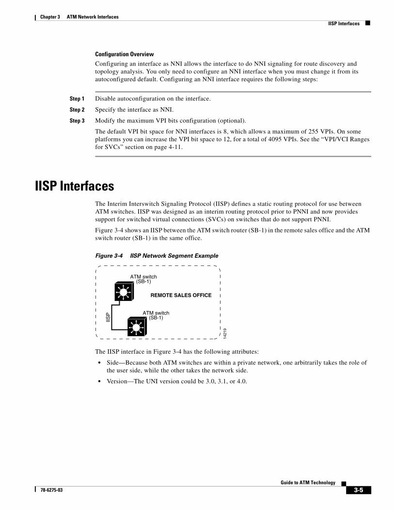
Chapter 3 ATM Network InterfacesIISP Interfaces
Configuration Overview
Configuring an interface as NNI allows the interface to do NNI signaling for route discovery and topology analysis. You only need to configure an NNI interface when you must change it from its autoconfigured default. Configuring an NNI interface requires the following steps:
Step 1 Disable autoconfiguration on the interface.
Step 2 Specify the interface as NNI.
Step 3 Modify the maximum VPI bits configuration (optional).
The default VPI bit space for NNI interfaces is 8, which allows a maximum of 255 VPIs. On some platforms you can increase the VPI bit space to 12, for a total of 4095 VPIs. See the “VPI/VCI Ranges for SVCs” section on page 4-11.
IISP InterfacesThe Interim Interswitch Signaling Protocol (IISP) defines a static routing protocol for use between ATM switches. IISP was designed as an interim routing protocol prior to PNNI and now provides support for switched virtual connections (SVCs) on switches that do not support PNNI.
Figure 3-4 shows an IISP between the ATM switch router (SB-1) in the remote sales office and the ATM switch router (SB-1) in the same office.
Figure 3-4 IISP Network Segment Example
The IISP interface in Figure 3-4 has the following attributes:
• Side—Because both ATM switches are within a private network, one arbitrarily takes the role of the user side, while the other takes the network side.
• Version—The UNI version could be 3.0, 3.1, or 4.0.
IISP
REMOTE SALES OFFICE
1421
9
ATM switch(SB-1)
ATM switch(SB-1)
3-5Guide to ATM Technology
78-6275-03

Chapter 3 ATM Network InterfacesIISP Interfaces
Configuration Overview
You only need to configure an IISP interface when you want to do static routing rather than the autoconfigured PNNI protocol that runs by default over NNI interfaces. Configuring an IISP interface requires the following steps:
Step 1 Disable autoconfiguration on the interface.
Step 2 Configure the interface as IISP and specify the UNI side and version.
Because there is no ILMI on IISP interfaces, these parameters must be manually configured. One interface is the user side, while the other is the network side. The versions should match on both devices.
Step 3 Configure the ATM route address prefix.
Specify the 13-byte address prefix of the destination interface for the static route.
For further information on IISP configuration, see Chapter 7, “ATM Routing with IISP and PNNI.”
3-6Guide to ATM Technology
78-6275-03

78-6275-03
C H A P T E R 4
Virtual ConnectionsThis chapter provides an overview of virtual connections, their characteristics and applications, and a functional explanation of each type of virtual connection. These explanations are accompanied by steps to provide a high-level overview of configuration.
Note The information in this chapter is applicable to the Catalyst 8540 MSR, Catalyst 8510 MSR, and LightStream 1010 ATM switch routers. For detailed configuration information, refer to the ATM Switch Router Software Configuration Guide and the ATM Switch Router Command Reference publication.
This chapter includes the following sections:
• Understanding ATM Virtual Connections, page 4-1
• PVCCs, page 4-5
• PVPCs, page 4-7
• Soft PVCs, page 4-8
• Nondefault Well-Known PVCCs, page 4-11
• VPI/VCI Ranges for SVCs, page 4-11
• VP Tunnels, page 4-13
Understanding ATM Virtual ConnectionsA virtual connection is established as a bidirectional facility to transfer ATM traffic between two ATM layer users. The following sections provide basic information about the types of ATM virtual connections, their applications, and their autonegotiated parameters.
4-1Guide to ATM Technology

Chapter 4 Virtual ConnectionsUnderstanding ATM Virtual Connections
Types of Virtual ConnectionsATM provides two kinds of virtual connection services, permanent and switched. Permanent virtual connections (PVCs), are manually set up and remain up until manually torn down. Following are the two main types of PVCs:
• Permanent virtual channel connections (PVCCs), specified by a virtual path identifier (VPI) and a virtual channel identifier (VCI)
• Permanent virtual path connections (PVPCs), specified by a VPI only
Both PVCCs and PVPCs can support point-to-point and point-to-multipoint connections.
Switched virtual connections (SVCs) are set up through signaling and remain up only as long as they are in use. Following are the two main types of SVCs:
• Switched virtual channels (SVCCs), specified by a VCI/VPI
• Switched virtual paths (SVPCs), specified by a VPI
Both SVCCs and SVPCs also support point-to-point and point-to-multipoint connections.
Soft PVCs, which includes soft PVCCs and soft PVPCs, are a hybrid between switched and permanent connections. Soft PVCs are specified by source and destination VPI/VCI values and the destination ATM address. They are then set up through signaling but, unlike SVCs, remain up until manually torn down.
Transit and Terminating ConnectionsFrom the standpoint of the ATM switch router, virtual connections can be further characterized as transit or terminating connections. Transit connections are switched from the ingress to the egress of the connection, while terminating connections terminate at the ATM switch router. Terminating connections usually end on the CPU interface and are used for management and signaling purposes, though the endpoint of a normal data connection can also be considered as terminating.
Connection ComponentsFigure 4-1 shows an example virtual channel connection (VCC) between ATM user A and user D. The end-to-end VCC has two parts:
• Virtual channel links, labelled VCL. These are the interconnections between switches, either directly or through VP tunnels.
• Internal connections, shown by the dotted line in the switch. These connections are also sometimes called cross-connections or cross-connects.
The common endpoint between an internal connection and a link occurs at the switch interface. The endpoint of the internal connection is sometimes referred to as a connection leg or half-leg. A cross-connect connects two legs together.
4-2Guide to ATM Technology
78-6275-03
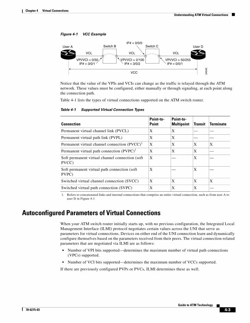
Chapter 4 Virtual ConnectionsUnderstanding ATM Virtual Connections
Figure 4-1 VCC Example
Notice that the value of the VPIs and VCIs can change as the traffic is relayed through the ATM network. These values must be configured, either manually or through signaling, at each point along the connection path.
Table 4-1 lists the types of virtual connections supported on the ATM switch router.
Autoconfigured Parameters of Virtual ConnectionsWhen your ATM switch router initially starts up, with no previous configuration, the Integrated Local Management Interface (ILMI) protocol negotiates certain values across the UNI that serve as parameters for virtual connections. Devices on either end of the UNI connection learn and dynamically configure themselves based on the parameters received from their peers. The virtual connection-related parameters that are negotiated via ILMI are as follows:
• Number of VPI bits supported—determines the maximum number of virtual path connections (VPCs) supported.
• Number of VCI bits supported—determines the maximum number of VCCs supported.
If there are previously configured PVPs or PVCs, ILMI determines these as well.
User A
VCC
VCL
VPI/VCI = 0/50IF# = 3/0/1
VCLVCL
VPI/VCI = 50/255 IF# = 0/0/1
IF# = 0/0/0
VPI/VCI = 2/100IF# = 3/0/2
Switch B Switch C User D
2454
2
Table 4-1 Supported Virtual Connection Types
Connection Point-to-Point
Point-to-Multipoint Transit Terminate
Permanent virtual channel link (PVCL) X X — —
Permanent virtual path link (PVPL) X X — —
Permanent virtual channel connection (PVCC)1
1. Refers to concatenated links and internal connections that comprise an entire virtual connection, such as from user A to user D in Figure 4-1
X X X X
Permanent virtual path connection (PVPC)1 X X X —
Soft permanent virtual channel connection (soft PVCC)
X — X —
Soft permanent virtual path connection (soft PVPC)
X — X —
Switched virtual channel connection (SVCC) X X X X
Switched virtual path connection (SVPC) X X X —
4-3Guide to ATM Technology
78-6275-03

Chapter 4 Virtual ConnectionsUnderstanding ATM Virtual Connections
Applications for Virtual ConnectionsThe application of various virtual connection types is summarized as follows:
• PVCs (PVCCs and PVPCs) connect to a node that needs quick access without signaling delay. Examples include the following:
– DNS server connections
– Terminating point-to-point and point-to-multipoint connections
– Any connection that needs to stay up permanently; for example, to connect buildings
– VP tunnels, which can connect through a public network without signaling
• SVCs (SVCCs and SVPCs) connect to a node that requires longer data exchanges but infrequent connections. Examples include the following:
– E-mail server
– CAD/CAM server
– Any connection that must be established on demand, such as LAN emulation
– Connections that require VPI/VCI values within a specific range (for special applications or interworking with nonstandard equipment)
• Soft PVCs, like hard PVCs, are permanent connections and have similar applications. However, they offer the advantages of setup with minimal manual configuration and the ability to reroute a connection if failure occurs. In this respect, soft virtual connections are considered more robust than hard virtual connections.
The main practical difference between a PVC and a soft PVC is that a soft PVC is automatically rerouted if a switch or link in the path fails. From that perspective a soft PVC is considered more robust than a hard PVC.
The difference between an SVC and a soft PVC is that an SVC is established on an “as needed” basis through user signaling. With a soft PVC the called party cannot drop the connection.
4-4Guide to ATM Technology
78-6275-03

Chapter 4 Virtual ConnectionsPVCCs
PVCCsThe following sections provide a general procedure for configuring PVCCs and example scenarios with PVCCs.
General Procedure for Configuring PVCCConfiguring a PVCC, such as the one shown in Figure 4-1, requires the following steps:
Step 1 Configure the connection traffic table rows (optional).
The connection traffic table specifies traffic management parameters for a connection. See the “Connection Traffic Table” section on page -3.
Step 2 Select the interface to configure and enter interface configuration mode.
Step 3 Configure the PVCC by mapping the source VPI/VCI values to the destination interface and VPI/VCI values. Do this for each cross-connect.
Using the example in Figure 4-1, you connect VPI/VCI 0/50 on interface 3/0/1 to VPI/VCI 2/100 on interface 3/0/2, and VPI/VCI 2/100 on interface 0/0/0 to VPI/VCI 50/255 on interface 0/0/1. Notice that the VPI/VCI values change on the cross-connect segment, but are the same at each end of a link between two systems.
Tips The VPI and VCI values at both ends of a link segment, for example, interface 3/0/2 on switch B and interface 0/0/0 on switch C, must match.
Terminating PVCCsTerminating connections provide internal connections to the ATM switch router’s route processor for LAN emulation (LANE), IP over ATM, and control channels for Integrated Local Management Interface (ILMI), signaling, and Private Network-to-Network Interface (PNNI) plus network management.
4-5Guide to ATM Technology
78-6275-03
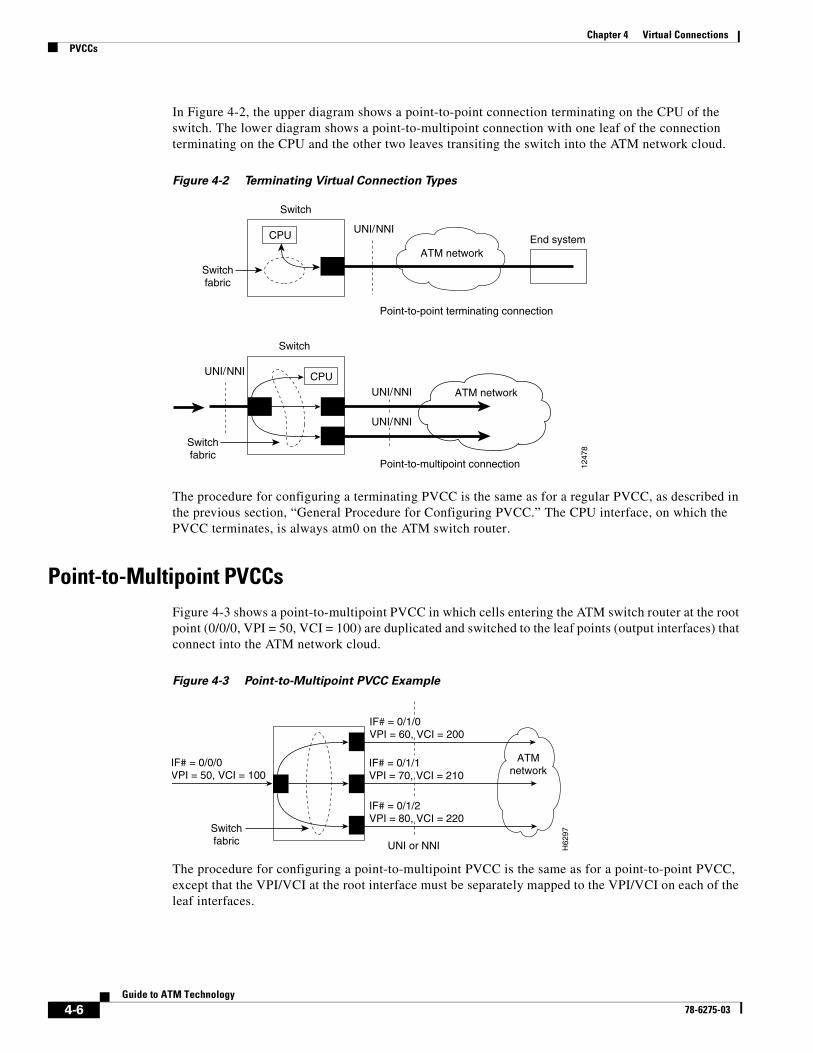
Chapter 4 Virtual ConnectionsPVCCs
In Figure 4-2, the upper diagram shows a point-to-point connection terminating on the CPU of the switch. The lower diagram shows a point-to-multipoint connection with one leaf of the connection terminating on the CPU and the other two leaves transiting the switch into the ATM network cloud.
Figure 4-2 Terminating Virtual Connection Types
The procedure for configuring a terminating PVCC is the same as for a regular PVCC, as described in the previous section, “General Procedure for Configuring PVCC.” The CPU interface, on which the PVCC terminates, is always atm0 on the ATM switch router.
Point-to-Multipoint PVCCsFigure 4-3 shows a point-to-multipoint PVCC in which cells entering the ATM switch router at the root point (0/0/0, VPI = 50, VCI = 100) are duplicated and switched to the leaf points (output interfaces) that connect into the ATM network cloud.
Figure 4-3 Point-to-Multipoint PVCC Example
The procedure for configuring a point-to-multipoint PVCC is the same as for a point-to-point PVCC, except that the VPI/VCI at the root interface must be separately mapped to the VPI/VCI on each of the leaf interfaces.
UNI/NNI
1247
8
End system
Switch
Switchfabric
CPU
ATM network
CPU
Point-to-multipoint connection
Point-to-point terminating connection
UNI/NNI
Switch
ATM networkUNI/NNI
UNI/NNI
Switchfabric
H62
97
UNI or NNI
ATM network
IF# = 0/1/1VPI = 70, VCI = 210
IF# = 0/1/0VPI = 60, VCI = 200
IF# = 0/0/0VPI = 50, VCI = 100
IF# = 0/1/2VPI = 80, VCI = 220
Switchfabric
4-6Guide to ATM Technology
78-6275-03

Chapter 4 Virtual ConnectionsPVPCs
PVPCsFigure 4-4 shows an example of PVPCs through the ATM switch routers connecting user A and user D. Because these are PVPCs, not PVCCs, they are identified by only VPIs.
Figure 4-4 PVPC Example
Configuration Overview
Configuring a PVPC, such as the one shown in Figure 4-4, requires the following steps:
Step 1 Configure the connection traffic table rows (optional).
The connection traffic table is used to specify traffic management parameters for a connection. See the “Connection Traffic Table” section on page -3.
Step 2 Select the interface to configure and enter interface configuration mode.
Step 3 Configure the PVPC by mapping the source VPI value to the destination interface and VPI value. Do this for each cross-connect.
Using the example in Figure 4-4, you would connect VPI 1 on interface 3/0/1 to VPI 2 on interface 3/0/2, and VPI 2 on interface 0/0/0 to VPI 50 on interface 0/0/1. The VPI values change on the cross-connect segment, but not on the link.
Point-to-Multipoint PVPCsFigure 4-5 shows a point-to-multipoint PVPC in which cells entering the ATM switch router at the root point (VPI = 50), are duplicated and switched to the leaf points (output interfaces).
Figure 4-5 Point-to-Multipoint PVPC Example
User A
PVP
VPL
VPI = 1IF# = 3/0/1
VPLVPL
VPI = 50 IF# = 0/0/1
IF# = 0/0/0
VPI = 2IF# = 3/0/2
Switch B Switch C User D
2454
3
H62
96
UNI or NNI
ATMnetwork
IF# = 0/1/1VPI = 70
IF# = 0/1/0VPI = 60
IF# = 0/0/0VPI = 50
IF# = 0/1/2VPI = 80
Switchfabric
4-7Guide to ATM Technology
78-6275-03

Chapter 4 Virtual ConnectionsSoft PVCs
The procedure for configuring a point-to-multipoint PVPC is the same as for a point-to-point PVPC, except that the VPI at the root interface must be separately mapped to the VPI on each of the leaf interfaces.
Soft PVCs The following sections provide examples and an overview of configuring soft PVCCs and soft PVPCs.
Soft PVCCsFigure 4-6 illustrates a soft PVCC connecting user A and user D through the ATM network cloud. Unlike hard PVCCs, the interface and VPI/VCI identifiers are needed only for the endpoints of the connection; the values for the intermediate switching points are not needed for the configuration, as these are determined by signaling.
Figure 4-6 Soft PVCC Example
Configuration Overview
Configuring a soft PVC, such as the one shown in Figure 4-6, requires the following steps:
Step 1 Configure the connection traffic table rows (optional).
The connection traffic table specifies traffic management parameters for a connection. See the “Connection Traffic Table” section on page -3.
Step 2 Decide which of the two connection endpoints you want to designate as the destination (or passive) side of the soft PVC.
This decision is arbitrary—it makes no difference which port you define as the destination end of the circuit.
Step 3 Retrieve the ATM address of the destination end of the soft PVC.
Step 4 Retrieve the currently used VPI/VCI values at both ends.
You must select unused VPI/VCI values for the connection.
Step 5 At the source end interface, specify a soft PVC with unused VPI/VCI values to the ATM address and VPI/VCI values of the destination interface.
Using the example in Figure 4-6, you would connect VPI/VCI 0 200 on interface 0/0/0 to the destination address 47.0091.8100.00.0000.1111.1111.1111.1111.1111.1111.00 with VPI/VCI 0 100.
2424
4
User A Switch B User DSwitch C
ATM network
IF# = 0/0/0VPI = 0, VCI = 200
IF# = 3/0/0VPI = 0, VCI = 100
Address = 47.0091.8100.0000.1111.1111.1111.1111.1111.1111.00
4-8Guide to ATM Technology
78-6275-03

Chapter 4 Virtual ConnectionsSoft PVCs
Soft PVPCsFigure 4-7 illustrates a soft PVPC that connects user A and user D through the ATM network cloud. The information needed to configure the soft PVPC is similar to that for a soft PVCC, except that only VPI values are used as connection identifiers.
Figure 4-7 Soft PCPC Example
The procedure for configuring a soft PVPC is identical to that used for a soft PVCC, except that no VCI values are used.
Route Optimization for Soft PVCsPVCs typically have a much longer life than switched virtual connections. This means that the route chosen, for example, during connection setup remains the same even though the topology of the network can change over time, making the original route less than optimal. With route optimization for soft PVCCs and soft PVPCs, the route can be recomputed periodically based on the following parameters:
• Time—a specified time period during which route optimization should be performed, and a time interval at which routes should be recomputed
• Threshold—a specified percentage by which an alternative route must represent an improvement over the existing route for route optimization to be triggered
At the specified time, all of the soft PVCs on the interface are checked to see if a better route exists. They are only rerouted if there is an available route that passes any QoS requirements and has a cumulative administrative weight that is better than the existing route by a percentage determined by the configured route-optimization percentage-threshold value (default 30 percent). Administrative weight is similar to hop count. For a description of administrative weight, see the “Administrative Weight—Global Mode and Per-Interface Values” section on page 7-30.
The route optimization feature applies to soft PVCCs and soft PVPCs on both ATM and Frame Relay interfaces.
User A Switch B User DSwitch C
2454
5ATM network
IF# = 0/0/0, VPI = 75Address = 47.0091.8100.0000.0000.0000.0000.0000.0000.0000.00
IF# = 3/0/0, VPI = 50Address = 47.0091.8100.0000.1111.1111.1111.1111.1111.1111.00
4-9Guide to ATM Technology
78-6275-03

Chapter 4 Virtual ConnectionsSoft PVCs
Configuration Overview
Configuring the route optimization feature for soft PVCs requires the following steps:
Step 1 From global configuration mode, enable route optimization and specify a threshold value.
Step 2 Select the interface to configure and enter interface configuration mode. You configure route optimization on the source end only of a soft PVC.
Step 3 Specify during what time of day and how often routes should be recomputed on this interface.
You can also manually trigger route optimization on a specific soft PVC.
Note Route optimization for soft PVCs should not be configured with constant bit rate (CBR) connections.
Soft PVCs with Explicit PathsPNNI performs dynamic routing of calls using soft PVCCs and soft PVPCs that are automatically set up over paths that meet the traffic parameter objectives. However, manually configured paths can be used in cases where a fully or partially specified explicit path is preferred. This feature is further described in the “Manually Configured Explicit Paths” section on page 7-29.
The explicit paths are assigned using precedence numbers 1 through 3. The precedence 1 path is tried first; if it fails the soft connection is routed using the precedence 2 path, and so forth. If all of the explicit paths fail, standard on-demand PNNI routing is tried unless routing has been configured to only use explicit paths.
An explicit path is defined using a series of entries. If the soft connection destination address is reachable at one of the included entries in an explicit path, any subsequent entries in that path are automatically disregarded. This allows longer paths to be reused for closer destinations. It is also possible to specify a point in the entries beyond which further path entries should be disregarded.
You can add, modify, or remove explicit paths without tearing down existing soft connections. When you redo a soft connection, you specify the VPI and VCI values; all applicable explicit path options are replaced by the respecified explicit path options.
The soft connection is not immediately rerouted using the new explicit path. However, reroutes using the new explicit path can happen for the following four reasons:
1. A failure occurs along the current path.
2. Route optimization has been enabled for the soft connection.
3. Route optimization has been enabled on the interface and the retry time interval has expired.
4. The soft PVC is disabled and then reenabled.
4-10Guide to ATM Technology
78-6275-03

Chapter 4 Virtual ConnectionsNondefault Well-Known PVCCs
Nondefault Well-Known PVCCsATM needs to set up and maintain well-known virtual connections for purposes such as signaling and management. Normally the default well-known virtual connections are automatically created with the default VCIs defined by the standards. In unusual circumstances, however, you can configure nondefault well-known VCI values on a per-interface basis. Two possible instances in which you might configure nondefault well-known VCI values are:
• When the ATM switch router connects with nonstandard equipment
• When the ATM switch router connects with service providers who offer SVC service and need multiple signaling channels
Table 4-2 lists the well-known PVVCs and their default VPI/VCI values.
Caution Do not swap virtual channel values between two types of well-known VCs.
Configuration Overview
Following is an overview of the steps needed to configure nondefault well-known virtual connections:
Step 1 Display the currently configured well-known virtual connections on the interface.
Step 2 Delete any existing automatically created well-known virtual connections on the interface.
Step 3 Configure the new VPI/VCI values on the interface and specify the encapsulation type (QSAAL, ILMI, PNNI, tag).
Step 4 Save these changes to your startup configuration file so that they are not lost if the switch reboots.
VPI/VCI Ranges for SVCsVPI/VCI conflicts can inadvertently occur when setting up SVCCs and SVPs. For example, suppose you specify a soft PVCC with VPI 0 and VCI 50 on the destination interface. An SVCC on that interface might have already taken VPI 0 and VCI 50 just before the soft PVCC setup message arrives at the destination interface. In this case, the soft PVCC is rejected because VPI 0 and VCI 50 are already taken.
Table 4-2 Well-Known Virtual Channels
Channel Type Virtual Path Identifier Virtual Channel Identifier
Connection control signaling (QSAAL)
0 5
ILMI 0 16
PNNI 0 18
Tag switching 0 32
4-11Guide to ATM Technology
78-6275-03

Chapter 4 Virtual ConnectionsVPI/VCI Ranges for SVCs
Specifying the VPI/VCI range for SVCs allows you to avoid such connection setup rejections. ILMI 4.0 uses this range when negotiating the VPI/VCI values for switched connections. Even if you specify a range, you can still configure PVCCs and PVPCs of any supported value, including any VPI/VCI range you configured for SVCCs and SVPCs.
The default maximum VPI for an SVPC or SVCC is 255. For interfaces configured with a 12-bit VPI space (NNI only) the default maximum is 4095. See Table 4-3.
Note The maximum value specified applies to all interfaces except logical interfaces, which have a fixed value of 0.
You can change the maximum VPI value. For example, in Figure 4-8 the maximum SVPC VPI is configured as 100. Therefore, VPIs 1 to 100 are reserved for SVPCs. You can use VPIs 101 to 255 for PVPCs; however, you are not restricted to that range.
Figure 4-8 Example SVPC VPI Range
Note In Figure 4-8 the maximum available VPI value would be 4095 instead of 255 for ports configured with a 12-bit VPI.
The default maximum VCI for an SVCC is 255, and the default minimum VCI for an SVCC is equal to 35. However, you can also change the minimum SVCC VCI. In the example shown in Figure 4-9, the maximum SVCC VPI is 100 and the minimum SVCC VCI is 60. Therefore, VPIs 0 through 100 and VCIs 60 through 16,383 are reserved for SVCCs.
Table 4-3 Maximum SVP VPI Ranges
VPI Bit Type Maximum Value Range
8-Bit VPI 0-255
12-Bit VPI1
1. 12-bit VPI configuration is available for NNI interfaces only on the Catalyst 8540 MSR.
0-4095
Max VPI
Max SVPC VPI 100
1
1011
10=no SVPCs 16,383Max VCI
Reservedfor SVPCs
255
VPI
VPI
4-12Guide to ATM Technology
78-6275-03

Chapter 4 Virtual ConnectionsVP Tunnels
Figure 4-9 Example SVCC VPI/VCI Range
Note In Figure 4-9 the maximum available VPI value would be 4095 instead of 255 for ports configured with a 12-bit VPI.
Every interface negotiates the local values for the maximum SVPC VPI, maximum SVCC VPI, and minimum SVCC VCI with the peer’s local value during ILMI initialization. The negotiated values determine the ranges for SVPCs and SVCCs. If the peer interface does not support these objects or autoconfiguration is turned off on the local interface, the local values determine the range.
Note The ATM router module has a default VCI space of 11 bits.
Configuration Overview
Configuring VPI/VCI ranges for SVPC and SVCCs requires the following steps at each interface where you need to specify a range:
Step 1 Select the interface to configure and enter interface configuration mode.
Step 2 Configure the maximum VPI value for SVPCs.
Step 3 Configure the maximum VPI value for SVCCs.
If you want to configure a maximum VPI greater than 255, then you must enable 12-bit VPIs on the interface. This option is platform dependent and is available on NNI interfaces only; see the configuration overview in the “NNI Interfaces” section on page 3-4.
Step 4 Configure the minimum VCI value for SVCCs.
VP TunnelsVirtual path (VP) tunnels provide the ability to interconnect ATM switch routers across public networks that do not support switched virtual connections. The VP tunnel uses a permanent virtual path (PVP) through the public network; signaling is done inside the PVP.
Max VPI
Max SVCC VPI 100
0
1011
26032 16,383Max VCI
Reservedfor SVCCs
255
Min SVCC VCI
VPI
VPI
4-13Guide to ATM Technology
78-6275-03
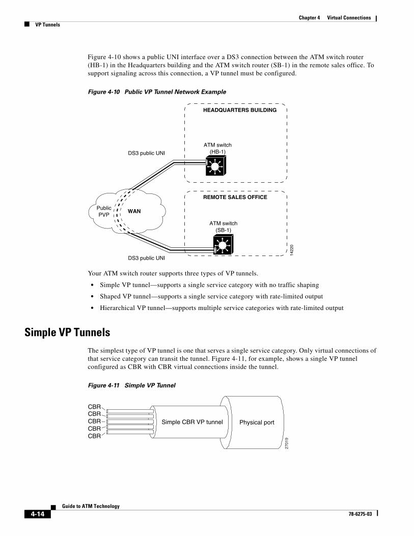
Chapter 4 Virtual ConnectionsVP Tunnels
Figure 4-10 shows a public UNI interface over a DS3 connection between the ATM switch router (HB-1) in the Headquarters building and the ATM switch router (SB-1) in the remote sales office. To support signaling across this connection, a VP tunnel must be configured.
Figure 4-10 Public VP Tunnel Network Example
Your ATM switch router supports three types of VP tunnels.
• Simple VP tunnel—supports a single service category with no traffic shaping
• Shaped VP tunnel—supports a single service category with rate-limited output
• Hierarchical VP tunnel—supports multiple service categories with rate-limited output
Simple VP TunnelsThe simplest type of VP tunnel is one that serves a single service category. Only virtual connections of that service category can transit the tunnel. Figure 4-11, for example, shows a single VP tunnel configured as CBR with CBR virtual connections inside the tunnel.
Figure 4-11 Simple VP Tunnel
HEADQUARTERS BUILDING
PublicPVP
REMOTE SALES OFFICE
WAN
1422
0
ATM switch(SB-1)
ATM switch(HB-1)DS3 public UNI
DS3 public UNI
Physical portSimple CBR VP tunnel
CBR
CBRCBR
CBRCBR
2701
9
4-14Guide to ATM Technology
78-6275-03

Chapter 4 Virtual ConnectionsVP Tunnels
You cannot use this type of VP tunnel to send traffic of varying service categories. If you have this requirement, you should use a hierarchical VP tunnel. Also, this type of VP tunnel is not a good choice if your service provider is policing the traffic on your leased bandwidth. If you have this requirement, you should consider a shaped or hierarchical VP tunnel.
Note Simple VP tunnels do not support interface overbooking.
Configuration Overview
Configuring a VP tunnel for a single service category without traffic shaping requires the following steps:
Step 1 Configure the connection traffic table rows (optional).
The connection traffic table specifies traffic management parameters for a connection. See the “Connection Traffic Table” section on page -3.
Step 2 Select the interface to configure and enter interface configuration mode.
Step 3 Configure a PVP on the interface with a VPI value.
Step 4 From global configuration mode, create a tunnel using the VPI of the PVP as the subinterface number.
Shaped VP TunnelsA shaped VP tunnel is configured as a PVP of the CBR service category. By default, this VP tunnel carries virtual connections only of the CBR service category. However, it is possible to configure a shaped VP tunnel to carry virtual connections of other service categories by substituting the new service category after the tunnel interface has been initially configured. The bandwidth of the shaped VP tunnel is shared by the active virtual connections inside the tunnel in strict round-robin (RR) fashion.
Figure 4-12 shows two shaped VP tunnels configured on a single physical port. One of the VP tunnels carries virtual connections of the default CBR service category; the other VP tunnel carries virtual connections of the UBR service category.
Figure 4-12 Shaped VP Tunnels
The overall output of this VP tunnel is rate-limited by hardware to the peak cell rate (PCR) of the tunnel. This feature is useful and often necessary when sending traffic through a public network using leased bandwidth that might be policed by the service provider.
Physical port
Shaped CBRVP tunnel
Shaped CBRVP tunnel
CBRCBRCBR
UBRUBR
UBR
2702
0
4-15Guide to ATM Technology
78-6275-03

Chapter 4 Virtual ConnectionsVP Tunnels
Restrictions on Shaped VP Tunnels
Shaped VP tunnels have the following restrictions:
• Shaped VP tunnels are not supported on systems with the FC-PCQ.
• Shaped VP tunnels do not support merged VCs for tag switching. If you need to support merged VCs, you can use a hierarchical VP tunnel.
• UBR+ and ABR VCs with non-zero minimum cell rate (MCR) are not allowed on a shaped VP tunnel interface. If you need to support these traffic categories, you can use a hierarchical VP tunnel.
• A maximum of 128 virtual connections can transit a shaped VP tunnel interface.
• There are platform-specific restrictions on the interfaces and the number of shaped VP tunnels that can be configured. Refer to the ATM Switch Router Software Configuration Guide for details.
Configuration Overview
Configuring a shaped VP tunnel requires the following steps:
Step 1 Configure a CBR connection traffic table row with the desired peak cell rate (PCR).
The connection traffic table is used to specify traffic management parameters for a connection. See the “Connection Traffic Table” section on page -3.
Step 2 Select the interface to configure and enter interface configuration mode.
Step 3 Configure a PVP on the interface with a VPI value.
Step 4 From global configuration mode, create a shaped tunnel using the VPI of the PVP as the subinterface number.
Hierarchical VP TunnelsA hierarchical VP tunnel allows virtual connections of multiple service categories to pass through the tunnel. In Figure 4-13, for example, hierarchical VP tunnels, configured as CBR, carry virtual connections of all five different service categories.
Figure 4-13 Hierarchical and Shaped VP Tunnels
Physical port
Hierarchical CBRVP tunnel
CBRVBr-rt
VBR-nrtABRUBR
Hierarchical CBRVP tunnel
CBRVBr-rt
VBR-nrtABRUBR
2702
1
4-16Guide to ATM Technology
78-6275-03
Chapter 4 Virtual ConnectionsVP Tunnels
The overall output of the VP tunnel is rate-limited to the PCR of the PVP. There is no general limit on the number of connections allowed on such a tunnel. Hierarchical VP tunnels can also support merged virtual connections for tag switching.
Hierarchical VP tunnels support the following service categories:
• Constant bit rate (CBR)
• Variable bit rate (VBR)
• Available bit rate (ABR) with a nonzero MCR
• Unspecified bit rate (UBR+) with a nonzero MCR
While capable of carrying any traffic category, a hierarchical VP tunnel is itself defined as CBR with a PCR.
Restrictions on Hierarchical VP Tunnels
Hierarchical VP tunnels have the following restrictions:
• Hierarchical VP tunnels are not supported on systems with the FC-PCQ.
• A hierarchical VP tunnel cannot coexist on a physical interface with other VP tunnels or other virtual connections, including tag switching.
• Either merged virtual connections for tag switching or ATM Forum virtual connections can be carried inside the hierarchical tunnel, but not both simultaneously.
• Bandwidth allocated on output to a hierarchical VP tunnel cannot be used by another hierarchical VP tunnel.
• You cannot add new hierarchical VP tunnels on a physical interface if the interface’s bandwidth guarantees exceed the MaxCR, regardless of any overbooking configured on that interface. See the “Interface Overbooking” section on page 10-12.
• There are platform-specific restrictions on the interfaces and number of hierarchical VP tunnels that can be configured. Refer to the ATM Switch Router Software Configuration Guide for details.
Configuration Overview
Configuring a hierarchical VP tunnel requires the following steps:
Step 1 Enable hierarchical mode globally and save the configuration.
Step 2 Reload the ATM switch router.
Caution When you reload the ATM switch router, all active connections are lost.
Step 3 Configure the connection traffic table row with the desired CBR PCR.
The connection traffic table specifies traffic management parameters for a connection. See the “Connection Traffic Table” section on page -3.
Step 4 Select the interface to configure and enter interface configuration mode.
Step 5 Configure a PVP on the interface with a VPI value.
Step 6 From global configuration mode, create a hierarchical tunnel using the VPI of the PVP as the subinterface number.
4-17Guide to ATM Technology
78-6275-03

Chapter 4 Virtual ConnectionsVP Tunnels
PVCC to VP Tunnel ConnectionsThe end point of a PVCC usually needs to be configured to transit a VP tunnel interface once the interface has been configured.
Restrictions on Configuring PVCC to VP Tunnel Connections
The following restrictions apply to an end point of a PVC-to-PVP tunnel subinterface:
• The VPI number of the tunnel leg of any PVCC must match the subinterface number of the tunnel.
• For single service-category VP tunnels, the service class specified by the connection-traffic-table-row (CTTR) of any PVCCs must match the service category for the row(s) selected for the tunnel PVP (for simple VP tunnels), or the configured service category (for shaped VP tunnels). This restriction does not apply to VP tunnels configured for multiple service categories (hierarchical VP tunnels).
• For service classes other than UBR, the PCRs of all PVCCs must be within the PCR of the tunnel PVP. This setup requires new CTTR rows to be defined for CBR or VBR PVCCs, with peak cell rates that are less than the intended tunnel PVP.
Configuration Overview
Configuring a PVCC to a VP tunnel is similar to configuring other cross-connections, and requires the following steps:
Step 1 Enter interface configuration mode for the interface you want to connect to the VP tunnel.
Step 2 Configure the PVCC by associating its VPI and VCI values to the subinterface and VPI/VCI values for the VP tunnel.
Signaling VPCI for VP Tunnels and Virtual UNIWhen VPI values on VP tunnels or virtual UNI interfaces are remapped as they traverse a VP switch, signaling can fail. For example, a VP tunnel connection from an ATM switch router on VPI 2, VCI X, to a router with a VP switch in between, would have a signaling message with connection ID, VPI 2, VCI X. If the VP tunnel at the router end is on VPI 3, VCI X, the connection is refused. By configuring VPCI to 3, you can configure the signaling message explicitly to contain connection ID VPI 3, VCI X, instead of VPI 2, VCI X.
A similar situation occurs when a virtual UNI is configured. For example, multiple VP tunnels traversing a VP switch might all carry signaling on VPI 0, VCI X. But these get remapped at the VP switch to, for example, VPI 1, VCI X. The end system expects VPI 0, VCI X, so the signaling request fails.
This problem is solved by specifying a signaling virtual path connection identifier (VPCI). The signaling VPCI specifies the value that is to be carried in the signaling messages within a VP tunnel. The connection identifier information element (IE) is used in signaling messages to identify the corresponding user information flow. The connection identifier IE contains the VPCI and VCI.
Note By default, the VPCI is the same as the VPI on the ATM switch router.
4-18Guide to ATM Technology
78-6275-03

Chapter 4 Virtual ConnectionsVP Tunnels
Configuration Overview
Configuring the signaling VPCI requires the following steps:
Step 1 Select the subinterface (VP tunnel) to configure and enter interface configuration mode.
Step 2 Specify a VPCI value.
Configuring the VPCI with a value of 0 works in most circumstances.
4-19Guide to ATM Technology
78-6275-03

Chapter 4 Virtual ConnectionsVP Tunnels
4-20Guide to ATM Technology
78-6275-03

78-6275-03
C H A P T E R 5
Layer 3 Protocols over ATMOne of the most common uses of ATM switches is in the backbone of a campus or enterprise network, or in the core of a WAN. In such applications, native mode network-layer traffic and LAN traffic must be carried across the ATM network. This chapter presents common scenarios and discusses two of the protocols that provide solutions for these problems.
This chapter contains the following sections:
• Background, page 5-1
• Classical IP and Multiprotocol Encapsulation Over ATM, page 5-2
Note The information in this chapter is applicable to the Catalyst 8540 MSR, Catalyst 8510 MSR, and LightStream 1010 ATM switch routers. For detailed configuration information, refer to the ATM Switch Router Software Configuration Guide and the ATM Switch Router Command Reference publication.
BackgroundAs a campus backbone or core of a WAN, ATM provides reliable transport, efficiency of bandwidth utilization, and QoS. In a typical scenario, end stations connected to the ATM network via a router and sending network layer packets, such as IP, want to take advantage of ATM’s benefits while communicating with end stations behind the other router across the ATM cloud (Figure 5-1).
Figure 5-1 Traffic Across the ATM Cloud
In a typical backbone implementation of ATM, the ATM network must carry traffic that is connectionless and in a network layer protocol format, such as IP. IP data, for example, is formatted in packets, not cells; IP is typically carried over a broadcast medium such as Ethernet or Token Ring and uses IP rather than ATM addresses. The requirements for transport of IP, or other Layer 3 protocols, are therefore fundamentally different from ATM.
2326
4
5-1Guide to ATM Technology

Chapter 5 Layer 3 Protocols over ATMClassical IP and Multiprotocol Encapsulation Over ATM
Two main problems must be solved in carrying network layer protocol traffic across the ATM network (see Figure 5-2):
• Packet encapsulation—how the network layer protocol packets are packaged into ATM cells
• Address resolution—how an ATM network device finds the location of an IP address and connects to it
Figure 5-2 Native Mode versus LAN Emulation
Broadly speaking, there are three approaches available to solve the challenges that packet encapsulation and address resolution pose:
• Native mode operation—approaches that are based on protocols that define IP connectivity over ATM using an address resolution mechanism, and encapsulation of Layer 3 protocols in ATM cells. The protocols and resultant approaches are described in the “Classical IP and Multiprotocol Encapsulation Over ATM” section on page 5-2.
• LANE—a MAC-layer protocol used to provide transparent LAN services across the ATM network. An enhancement of LANE, Multiprotocol over ATM (MPOA) uses LANE technology with cut-through routing to improve performance in large networks. For descriptions of these protocols, see Chapter 6, “LAN Emulation and MPOA.”
• Tag switching—a technology that combines the benefits of routing with the performance of switching to offer another solution to forwarding IP packets over an ATM network. See Chapter 11, “Tag Switching.”
Classical IP and Multiprotocol Encapsulation Over ATMSeveral protocols have been designed to provide complementary mechanisms and formats that address the issues of address resolution and encapsulation. Two protocols in particular provide the basis for native mode transport of IP and other network layer protocols over ATM:
• “Classical IP and ARP over ATM” (RFC 1577)—defines an application of classical IP in an ATM network environment using switched virtual channel connections (SVCCs) and permanent virtual channel connections (PVCCs) and specifies mechanisms for address resolution and discovery.
• “Multiprotocol Encapsulation over ATM Adaptation Layer 5” (RFC 1483)—defines how various types of PDUs are encapsulated for transport over ATM.
IPIP
MACprotocols
ATMATM
LAN emulationNative mode 2339
5
5-2Guide to ATM Technology
78-6275-03

Chapter 5 Layer 3 Protocols over ATMClassical IP and Multiprotocol Encapsulation Over ATM
RFC 1577 ProvisionsIn the RFC 1577 model, ATM becomes a direct replacement for the interconnection of local LAN segments that contain IP end stations and routers operating in the classical LAN-based paradigm. Such LAN segments, called logical IP subnets (LISs), are identical in all “protocol” aspects to conventional LAN media subnets. ATM-attached systems in the same LIS have the same network numbers and subnet masks, just as on an Ethernet or other conventional media. Two ATM-attached systems not in the same LIS can communicate only through a router—hence the term “classical” IP—even though they are both attached to the same ATM physical network. RFC 1577 also specifies address resolution and discovery mechanisms. These are the ATM Address Resolution Protocol (ATMARP) and Inverse ATM Address Resolution Protocol (InATMARP).
The ATMARP Mechanism
In traditional LANs the function of finding a MAC layer address is performed by the ARP mechanism, which identifies the MAC address corresponding to an IP or other network layer address, and by the broadcast mechanism, which sends a single packet over the LAN that is seen by every device on the segment. This is not possible in ATM, since no such thing as a broadcast address exists. Additionally, ATM is point-to-point, so the only way to broadcast a single frame is to send copies of the same frame over every point-to-point link, addressed to the unique ATM address of that device.
RFC 1577 specifies that address resolution be accomplished by the ATMARP server, a centralized server that maintains a table of IP addresses to ATM addresses. The ARP server maintains this table for a single IP subnet, and any client that needs to communicate with another client can query the ARP server to get that device's ATM address and directly set up a connection to it.
How It Works
Figure 5-3 contains three ATMARP clients and one ATMARP server. When coming online, the ARP clients register their IP and ATM addresses with the ARP server.
Figure 5-3 Classical IP-Over-ATM Example
Router client C123.233.45.6
Switch client A123.233.45.1
Switch client B123.233.45.3
Switch ARP server123.233.45.2
ATM network123.233.45.0
1422
1
3
54
2
1
5-3Guide to ATM Technology
78-6275-03

Chapter 5 Layer 3 Protocols over ATMClassical IP and Multiprotocol Encapsulation Over ATM
The following sequence describes the process whereby a classical IP-over-ATM connection is set up between ATM switch router client A and client B:
1. The initial IP packet sent by client A triggers a request to the ARP server to look up the IP address and the corresponding ATM address of client B in the ARP table.
For each packet with an unknown IP address, the client sends an ATMARP request to the ARP server. Until that address is resolved, any IP packet routed to the ATM interface causes the client to send another ATMARP request.
2. The ARP server sends back a response to client A with the matching ATM address.
3. Client A uses the ATM address it just obtained from the ARP server to set up an SVCC directly to client B.
4. When client B replies with an IP packet to client A, it also triggers a query to the ARP server.
When client B receives the ATM address for client A, it usually discovers it already has a call set up to client A’s ATM address and does not set up another call.
5. Once the connection is known to both clients, they communicate directly over the SVCC.
In Cisco’s implementation, the ATMARP client tries to maintain a connection to the ATMARP server. The ATMARP server can tear down the connection, but the client attempts once each minute to bring the connection back up. No error message is generated for a failed connection, but the client will not route packets until the ATMARP server is connected and translates IP network addresses.
The ATM switch router can be configured as an ATMARP client to work with any ATMARP server conforming to RFC 1577. Alternatively, one of the ATM switch routers in an LIS can be configured to act as the ATMARP server itself. In that case, it automatically acts as a client as well.
Note When possible, we recommend placing the ATMARP server on a router rather than a switch.
The InATMARP Mechanism
With InATMARP there is no server function; rather, clients exchange information and discover one another’s protocol address. To discover the protocol address of the remote end of a connection, a client sends an InATMARP request over a virtual connection for the address of the other end; this is how a client knows what addresses it can reach. This mechanism provides an alternative to statically mapping ATM and IP addressees in the configuration.
RFC 1483 ProvisionsAs its name implies, multiprotocol encapsulation over ATM, defined in RFC 1483, provides mechanisms for carrying traffic other than just IP. RFC 1483 specifies two ways to do this:
• Logical Link Control (LLC)/Subnetwork Access Protocol (SNAP) encapsulation—in this method, multiple protocol types can be carried across a single connection with the type of encapsulated packet identified by a standard LLC/SNAP header.
• Virtual connection multiplexing—in this method, only a single protocol is carried across an ATM connection, with the type of protocol implicitly identified at connection setup.
5-4Guide to ATM Technology
78-6275-03

Chapter 5 Layer 3 Protocols over ATMClassical IP and Multiprotocol Encapsulation Over ATM
LLC encapsulation is provided to support routed and bridged protocols. In this encapsulation format, PDUs from multiple protocols can be carried over the same virtual connection. The type of protocol is indicated in the packet’s SNAP header. By contrast, the virtual connection multiplexing method allows for transport of just one protocol per virtual connection.
Static Map ListsStatic map lists belong to neither RFC 1483 nor RFC 1577 specifications. Rather, this is a Cisco IOS feature that offers an alternative to using the ATMARP or InATMARP mechanisms. With static maps lists, you can associate, among other things, a protocol address with an ATM address or with a VCI/VPI.
Figure 5-4 illustrates the use of static address mapping to set up a connection between switch A and switch B.
Figure 5-4 Multiprotocol Encapsulation over ATM Example
The following process occurs when a connection between switch A and switch B needs to be set up to forward an IP packet:
1. An IP packet with destination 123.233.45.3 arrives at switch A.
2. Switch A finds the destination IP address in its map list.
3. Using a statically configured map list, switch A identifies the ATM address corresponding to the next-hop IP address (for SVCCs) or the VPI/VCI value corresponding to the next-hop IP address (for PVCCs).
4. If SVCCs are used, signaling sets up a virtual connection to the destination ATM address. If PVCCs are used, the connection follows the statically configured path of the virtual connection.
5. The encapsulated packet is forwarded over the ATM virtual connection.
Common ImplementationsThe solutions found in RFC 1483, RFC 1577, and Cisco’s static map list feature, can be combined in various ways. Four of the most common of these, along with their advantages and limitations, are described in this section.
Router client C123.233.45.6
Switch client A123.233.45.1
Switch client B123.233.45.3
Switch ARP server123.233.45.2
ATM network123.233.45.0
1422
1
3
54
2
1
5-5Guide to ATM Technology
78-6275-03
Chapter 5 Layer 3 Protocols over ATMClassical IP and Multiprotocol Encapsulation Over ATM
SVCCs with ATMARP
The essential ingredients of this implementation are encapsulation of native protocol IP datagrams over ATM (in RFC 1483 routed IP format) and use of the RFC 1577 ATMARP mechanism to map IP addresses to ATM addresses (see the “The ATMARP Mechanism” section on page 5-3).
Advantages
Potential advantages of SVCCs with ATMARP include the following:
• Many vendors support the ATMARP function, making it is widely interoperable.
• For interconnecting IP subnets, it is less complex than LANE.
• Configuration in a small network is simple.
• A Cisco proprietary mechanism allows configuration of multiple ATMARP servers on the ATMARP clients, eliminating the liability of a single ATMARP server failure.
Limitations
Potential limitations of SVCCs with ATMARP include the following:
• No multicast capability is provided.
• Only the IP network protocol is supported.
• This implementation cannot take advantage of the router’s traffic shaping capability; therefore, this implementation might not be a good choice for sending traffic through a public network.
• Because address resolution is limited to a single hop and inter-LIS traffic must traverse a router, multiple hops are required for communication between different LISs. This can increase the load on the network resources, particularly as it results in repeated SARs.
• The ATMARP server is a single point of failure in the network.
• In a large network, configuring each host with its ATMARP server address can be tedious and can result in configuration errors.
PVCCs with InATMARP
In this implementation, static routes are configured between network devices (switches and routers) using PVCCs. The network protocol address of the remote end of a connection is not configured, but is discovered by the Inverse ATMARP (InATMARP) process. IP packets are encapsulated in SNAP, per RFC 1483.
Advantages
Potential advantages of PVCCs with InATMARP include the following:
• Many vendors support the InATMARP functions, making it widely interoperable.
• For interconnecting IP subnets, it is less complex than LANE.
Limitations
Potential limitations of PVCCs with InATMARP include the following:
• No multicast capability is provided.
• Only the IP network layer protocol is supported.
• This implementation cannot take advantage of the router’s traffic shaping capability; therefore, this implementation might not be a good choice for sending traffic through a public network.
5-6Guide to ATM Technology
78-6275-03

Chapter 5 Layer 3 Protocols over ATMClassical IP and Multiprotocol Encapsulation Over ATM
• Because address resolution is limited to a single hop and inter-LIS traffic must traverse a router, multiple hops are required for communication between different LISs. This can increase the load on the network resources, particularly as it results in repeated SARs.
• Because PVCCs are manually configured, the complexity of configuration and the possibility of error increase with the number of devices you have to configure.
PVCCs with Static Address Mapping
In this implementation PVCCs are configured between switches (or between switches and routers in a routed subnet design). Using statically configured map lists, each PVCC is mapped to a destination protocol address; packets are routed based on the mappings in the map list.
Advantages
Potential advantages of PVCCs with static mapping include the following:
• This implementation can support different Layer 3 protocols.
• Configuration is simple for a few nodes.
• Encapsulations is supported by many vendors.
Limitations
Potential limitations of this implementation include the following:
• Scalability is a problem, because the number of PVCCs to configure grows exponentially with the addition of nodes.
• It is strongly recommended not to use OSPF as routing protocol if the network is a meshed one that requires multicasting.
• With PVCCs, there is no dynamic reaction to ATM failures; a possible workaround is to use soft PVCCs.
• Bridged and routed 1483 cannot exist on the same PVCC, unless you enable Integrated Routing and Bridging (IRB) on the router.
SVCCs with Static Address Mapping
In this implementation SVCCs are set up as needed based on the information in the statically configured map list. That list contains mappings of protocol addresses to ATM addresses. To set up a connection to a destination protocol address, the ATM switch router locates the ATM address that corresponds to the protocol address in the map list, then sets up an SVCC to that ATM address.
Advantages
Potential advantages of SVCCs with static mapping include the following:
• The implementation can support different Layer 3 protocols.
• Encapsulation is supported by many vendors.
• Multicasting and broadcasting are supported on static map subinterfaces that are of type multipoint. Multipoint routing in the form of PIM is also supported in this environment.
5-7Guide to ATM Technology
78-6275-03

Chapter 5 Layer 3 Protocols over ATMClassical IP and Multiprotocol Encapsulation Over ATM
Limitations
Potential limitations of SVCCs with static mapping include the following:
• It is strongly recommended not to use OSPF as a routing protocol if the network is a meshed one that requires multicasting.
• The signaling complexity inherent in using SVCCs can be a troubleshooting liability.
In the WAN, this implementation might have the following additional limitations:
• There can be problems with signaling of SVCCs when connecting to a service provider’s address space. A possible alternative is to use SVCCs inside a VP tunnel.
• There is no point-to-multipoint support.
Scenarios for Inband ManagementThe implementations described above provide one set of solutions to the need posed in Figure 5-1. In this scenario, in which routed subnets are interconnected over ATM, the role of the ATM switch router is essentially a passive one. Encapsulation and address resolution take place on the routers, and the switches function only to forward ATM cells through the network on SVCCs or PVCCs.
In a primarily Layer 2 ATM switch environment, however, these solutions can be used for inband management of the ATM switch router. When the ATM switch router is managed with out-of-band connections, a separate Ethernet connection is required for each device. For example, if you have multiple switches to manage through SNMP, you would have connections to the Ethernet port on the CPU of each of the switches. By using an implementation from RFC 1577 and RFC 1483, you can connect to just one of those ports and get management information from all the others using interswitch SVCCs or PVCCs (see Figure 5-5). In this scenario, you are accessing management information through an inband (ATM) connection rather than by out-of-band (Ethernet) connection.
Figure 5-5 Inband Network Management
Some risk occurs in using the ATM network itself to provide network management connectivity. However, this liability can be mitigated if you have redundant links and multiple paths. For this reason, implementations with SVCCs might be preferable.
2326
5
SNMP
Switch A Switch BCPU Ethernet
port
Networkmanagement
station
5-8Guide to ATM Technology
78-6275-03

Chapter 5 Layer 3 Protocols over ATMClassical IP and Multiprotocol Encapsulation Over ATM
Typical Configurations for Inband Management
The configuration overviews in this section describe ways you can use solutions discussed in the “Common Implementations” section on page 5-5 for inband management of the ATM switch router.
SVCCs with ATMARP
The following steps describe configuring the ATM switch router as an ARP client, such as switch client A in Figure 5-5:
Step 1 Enable IP host-based routing on the ATM switch router.
This enables the switch to perform basic routing functions.
Step 2 Configure an ATM address on the processor’s ATM interface.
Step 3 Configure an IP address on the processor’s ATM interface.
Step 4 Specify the ATM address of the ARP server.
Step 5 Configure a static route through the ATM switch router to the processor interface.
This step is required only when configuring the ARP client using an NSAP form address; ESI format addresses do not require this step.
The following steps describe configuring the ATM switch router as an ARP server, such as switch B in Figure 5-5:
Step 1 Enable IP host based routing on the ATM switch router.
This enables the switch to perform basic routing functions.
Step 2 Configure an ATM address on the processor’s ATM interface.
Step 3 Configure an IP address on the processor’s ATM interface.
Step 4 Enable the ARP server on this device.
Step 5 Configure a static route through the ATM switch router to the processor interface.
This step is required only when configuring the ARP server using an NSAP format address; ESI format addresses do not require this step.
It might be useful to keep the following additional points in mind when setting up SVCCs with ATMARP:
• The size of the MTU must be the same for all nodes in the LIS. This parameter is negotiated, but there could be a mismatch when connecting with non-Cisco equipment, such as a UNIX workstation with an ATM NIC that supports the RFC 1577 protocol.
• All members of an LIS must be in the same IP network/subnet and have the same address mask.
• All members outside the LIS have to go through the router.
• There must be one ARP server per LIS.
5-9Guide to ATM Technology
78-6275-03

Chapter 5 Layer 3 Protocols over ATMClassical IP and Multiprotocol Encapsulation Over ATM
PVCCs with InATMARP
The following steps are required to configure PVCCs with InATMARP for inband management such as that in Figure 5-5:
Step 1 Enable IP host-based routing on the ATM switch router.
This enables the switch to perform basic routing functions.
Step 2 Configure an IP address on the processor’s ATM interface.
Step 3 Create a PVCC to the remote end.
Step 4 Enable InATMARP and SNAP encapsulation on the interface.
Keep the following additional points in mind when setting up PVCCs with InATMARP:
• The size of the MTU must be the same for all nodes in the LIS. Like the UNI version, this parameter is negotiated, but could fail when using non-Cisco equipment.
• All members of an LIS must be in the same IP subnet and must have the same address mask.
• All members outside the LIS have to go through a router.
PVCCs with Static Address Mapping
The following steps are required to configure a PVCC-based static IP address mapping on the ATM switch router for inband management, such as in Figure 5-5:
Step 1 Enable IP host-based routing on the ATM switch router.
This enables the switch to perform basic routing functions.
Step 2 Configure the IP address on the processor’s ATM interface.
Step 3 Specify a map-group name to associate with the PVCC you are setting up.
Step 4 Configure a PVCC and specify the encapsulation type.
Step 5 Make a map-list entry that maps the remote end’s IP address to the PVCC you set up in Step 4.
SVCCs with Static Address Mapping
The following steps are required to configure SVCC-based static IP address mapping on the ATM switch router for inband management, such as in Figure 5-5:
Step 1 Enable IP host-based routing on the ATM switch router.
This enables the switch to perform basic routing functions.
Step 2 Configure the IP address on the processor’s ATM interface.
Step 3 Configure the ATM address on the processor’s ATM interface.
Step 4 Specify a map-group name to associate with this interface.
Step 5 Make a map-list entry that maps the remote end’s IP address to its ATM address.
5-10Guide to ATM Technology
78-6275-03

78-6275-03
C H A P T E R 6
LAN Emulation and MPOAThis chapter provides an overview of LAN emulation and a related technology, Multiprotocol Over ATM (MPOA). The background and rationale for these protocols are discussed in Chapter 5, “Layer 3 Protocols over ATM.”
This chapter contains the following sections:
• LAN Emulation, page 6-1
• Multiprotocol over ATM, page 6-19
Note The information in this chapter is applicable to the Catalyst 8540 MSR, Catalyst 8510 MSR, and LightStream 1010 ATM switch routers. For detailed configuration information, refer to the ATM Switch Router Software Configuration Guide and the ATM Switch Router Command Reference publication.
LAN EmulationLAN emulation (LANE) is a standard defined by the ATM Forum that provides ATM-attached stations the same capabilities they normally obtain from legacy LANs, such as Ethernet and Token Ring. As the name suggests, the function of the LANE protocol is to emulate a LAN on top of an ATM network. By making an ATM interface look like one or more separate Ethernet or Token Ring interfaces, LANE allows LAN users to take advantage of ATM’s benefits without requiring modifications to end station hardware or software.
As Figure 6-1 illustrates, LANE uses ATM to replace the legacy LAN backbone. Multiple emulated LANs (ELANs), which are logically separated, can share the same physical ATM network and same physical ATM interface.
6-1Guide to ATM Technology

Chapter 6 LAN Emulation and MPOALAN Emulation
Figure 6-1 Physical and Emulated LANs
LANE ApplicationsLANE services provide connectivity between ATM-attached devices and LAN-attached devices. The following are two primary applications of LANE (see Figure 6-2):
• Connectivity between LAN-attached stations across an ATM network, effectively extending LANs over a high-speed ATM transport backbone.
• Connectivity between ATM-attached hosts and LAN-attached hosts. Centralized hosts with high-speed ATM interfaces can provide services, such as Domain Name System (DNS), to traditional LAN-attached devices.
Figure 6-2 LANE Applications
The following types of devices can be used to support LANE services:
• Directly attached ATM hosts with ATM NICs
• Layer 2 devices, such as switches with ATM interfaces or the ATM switch routers
• Layer 3 devices, such as routers with ATM interfaces
Emulated LAN
Physical LAN
1234
4
ATMnetwork
ATMnetwork
ATM end station(server with ATM NIC)
Routerwith ATM interface
LAN switchwith ATM LANE
LAN switchwith ATM LANEATM
switch
1422
8
6-2Guide to ATM Technology
78-6275-03

Chapter 6 LAN Emulation and MPOALAN Emulation
How It WorksATM is a connection-oriented service that uses point-to-point signaling or point-to-multipoint signaling to establish connections between source and destination devices. LAN-based protocols, on the other hand, are connectionless and use broadcasts so that source devices can find one or more destination devices. The primary purpose of LANE, then, is to provide the same services that a broadcast medium like Ethernet does.
The LANE protocol defines mechanisms for emulating either an IEEE 802.3 Ethernet or an 802.5 Token Ring LAN. Specifically, LAN broadcasts are emulated as ATM unicasts. The current LANE protocol does not define a separate encapsulation for Fiber Distributed Data Interface (FDDI). (FDDI packets must be mapped into either Ethernet or Token Ring emulated LANs by using existing translational bridging techniques.) Fast Ethernet (100BaseT) and IEEE 802.12 (100VG-AnyLAN) both can be mapped unchanged because they use the same packet formats.
LANE defines a service interface for network layer protocols that is identical to existing MAC layers. No changes are required to existing upper layer protocols and applications. However, LANE does not emulate every particular physical or data-link characteristic. For example, it does not support carrier sense multiple access collision detect (CSMA/CD) for either Ethernet or Token Ring. LANE clients on an ATM switch router only support the IP protocol.
The Function of ATM Network Devices
The basic function of the LANE protocol is to resolve MAC addresses to ATM addresses so that LANE end systems can set up direct connections between themselves and then forward data. The LANE protocol can be deployed in two types of ATM-attached equipment: ATM network interface cards (NICs) and LAN devices, such as switches and routers.
ATM NICs implement the LANE protocol and interface to the ATM network while presenting the current LAN service interface to the higher-level protocol drivers within the end system. The network-layer protocols on the end system continue to communicate as if they were on a known LAN, by using known procedures. However, they are able to take advantage of most of the advanced services of the ATM network.
The second class of network device that implements LANE consists of ATM-attached LAN switches and routers. These devices, together with directly attached ATM hosts equipped with ATM NICs, are used to provide a virtual LAN service in which ports are assigned to particular virtual LANs, independent of physical location. Figure 6-3 shows the LANE protocol stack used between these devices.
6-3Guide to ATM Technology
78-6275-03

Chapter 6 LAN Emulation and MPOALAN Emulation
Figure 6-3 LANE Protocol Stack
Ethernet and Token Ring Emulated LANs
The LANE version 1 standard defines separate emulated LANs for Ethernet and Token Ring, but does not explicitly define how to connect the two types directly. An ATM equipped router, such as the Cisco 7000 with an ATM interface, acting as a LANE client on each emulated LAN, can provide this connectivity while allowing the administrator to construct firewalls or to filter traffic between emulated LANs.
LANE Servers and Components
The LANE specification defines several components that enable the protocol to provide the broadcast and address resolution services required to emulate traditional LANs:
• LANE client (LEC)—An entity in an end system such as a workstation, LAN switch, or router that performs data forwarding and receiving, address resolution, and other control functions for a single endpoint in a single emulated LAN. The LEC provides a standard LAN service to any higher layers that interface to it. A router or switch can have multiple resident LECs, each connecting with different emulated LANs. The LANE client registers its MAC and ATM address with the LES. In Token Ring environments, a LANE client configured for source-route bridging can register a route descriptor with the LES.
• LANE server (LES)—A server that provides a registration facility for clients to join the emulated LAN. The LES handles LAN Emulation Address Resolution Protocol (LE_ARP) requests and maintains a list or look-up table of LAN destination MAC addresses. In Token Ring LANE environments, the LES maintains a list of route descriptors. Each emulated LAN must have an LES.
• Broadcast-and-unknown server (BUS)—A server that floods unknown destination traffic and forwards multicast and broadcast traffic to clients within an emulated LAN. Each emulated LAN must have a BUS.
Existingapplications
Driver l/f
LANE
AAL5
ATM
ATM host LAN hostATM switch ATM-capableLAN switch
Physical layer
ATM
Existingapplications
Driver l/f
MACMAC
Bridging
Physical layer
ATM
AAL5
LANE
Physicallayer
LANemulation
Physicallayer
Physicallayer
Physicallayer 12
502
6-4Guide to ATM Technology
78-6275-03

Chapter 6 LAN Emulation and MPOALAN Emulation
Note In Cisco’s LANE implementation, the LES and BUS are combined.
• LANE configuration server (LECS)—A server that assigns individual clients to particular emulated LANs by directing them to the LES that corresponds to the emulated LAN. The LECS maintains a database of LANE client ATM or MAC addresses and their emulated LANs. One LECS is required for each LANE cloud, but an LECS can serve multiple emulated LANs. The LECS can enforce security by restricting ELAN membership to certain LECs based on their MAC addresses.
These servers could be single points of failure in a LANE, but Cisco has developed a fault tolerance mechanism, known as Simple Server Redundancy Protocol (SSRP), which eliminates these single points of failure. Although this scheme is proprietary, no new protocol additions have been made to the LANE subsystems, which are described in the “SSRP for Fault-Tolerant Operation of LANE Server Components” section on page 6-17.
Comparing Virtual LANs and Emulated LANs
In the Catalyst family of switches, a virtual LAN (VLAN) is a logical group of end stations, independent of physical location, with a common set of requirements. Currently, the Catalyst switches support a port-centric VLAN configuration.
A VLAN is identified by a number, which is only significant to the Catalyst family of switches. On an ATM network, an emulated LAN is designated by a name. Therefore, the VLAN number must be mapped to the emulated LAN on the Catalyst switch. To create a VLAN that spans multiple Catalyst switches on an ATM network, you must assign the VLAN on each Catalyst switch to the same emulated LAN. Members of two or more different emulated LANs can communicate only through a router, whether they are on the same or different Catalyst switches.
LANE Virtual Connection Types
Communication among LANE components is ordinarily handled by several types of SVCCs. (In discussions of LANE, these SVCCs are commonly called virtual channel connections, or VCCs). Some VCCs are unidirectional; others are bidirectional. Some are point-to-point; others are point-to-multipoint. Figure 6-4 illustrates the various types of VCCs followed by a description of each.
6-5Guide to ATM Technology
78-6275-03

Chapter 6 LAN Emulation and MPOALAN Emulation
Figure 6-4 LANE VCC Types
Control direct VCC—The LEC, as part of its initialization, sets up a bidirectional point-to-point VCC to the LES for sending or receiving control traffic. The LEC is required to accept control traffic from the LES through this VCC and must maintain the VCC while participating as a member of the emulated LAN.
Control distribute VCC—The LES can optionally set up a unidirectional VCC back to the LEC for distributing control traffic. Whenever an LES cannot resolve an LE_ARP request from a LEC, it forwards the request out the control distribute VCC to all of the clients in the emulated LAN. The control distribute VCC enables information from the LES to be received whenever a new MAC address joins the LAN or whenever the LES cannot resolve an LE_ARP request.
Data direct VCC—Once an ATM address has been resolved by a LEC, this bidirectional point-to-point VCC is set up between clients that want to exchange unicast data traffic. Most client traffic travels through these VCCs.
Multicast send VCC—The LEC sets up a unidirectional point-to-point VCC to the BUS. This VCC is used by the LEC to send multicast traffic to the BUS for forwarding out the multicast forward VCC. The LEC also sends unicast data on this VCC until it resolves the ATM address of a destination.
Multicast forward VCC—The BUS sets up a unidirectional VCC to the LECs for distributing data from the BUS. This can either be a unidirectional point-to-point or unidirectional point-to-multipoint VCC. Data sent by a LEC over the multicast send VCC is forwarded to all LECs over the multicast forward VCC.
Configure direct VCC—This is a transient VCC set up by the LEC to the LECS for the purpose of obtaining the ATM address of the LES that controls the particular LAN the LEC wishes to join.
LE server
Client A
LECS
Client B
BUS
S37
36
1–72–83–11
Control direct Control distribute Configure direct (client)
4–95–106–611–12
Multicast send Multicast forward Data directConfigure direct (server)
1 2 3 4
5
6 6
2
1 3 5 4
910
911
78
7
1112
6-6Guide to ATM Technology
78-6275-03

Chapter 6 LAN Emulation and MPOALAN Emulation
Joining an Emulated LAN
The following sequence (see Figure 6-4) describes the normal process that occurs when a LEC requests to join an emulated LAN:
1. The LEC requests to join an emulated LAN.
The LEC sets up a connection to the LECS (bidirectional, point-to-point configure direct VCC, link 3-11 in Figure 6-4) to find the ATM address of the LES for its emulated LAN.
The LEC finds the LECS by using the following interface and addresses in the listed order:
– Statically configured ATM address
– ILMI (from directly attached ATM switch router)
– The well-known address (defined by the ATM Forum)
2. The LECS identifies the LES.
Using the same VCC, the LECS returns the ATM address and the name of the LES for the LEC’s emulated LAN.
3. The LEC tears down the configure direct VCC.
4. The LEC contacts the LES for its emulated LAN.
The LEC sets up a connection to the LES for its emulated LAN (bidirectional, point-to-point control direct VCC, link 1-7 in Figure 6-4) to exchange control traffic. When a control direct VCC is established between an LEC and an LES, it remains established.
5. The LES verifies that the LEC is allowed to join the emulated LAN.
The LES for the emulated LAN sets up a connection to the LECS to verify that the LEC is allowed to join the emulated LAN (bidirectional, point-to-point server configure VCC, link 11-12 in Figure 6-4); this is a Cisco proprietary action. The LES configuration request contains the LEC MAC address, its ATM address, and the name of the emulated LAN. The LECS checks its database to determine whether the LEC can join that emulated LAN; then it uses the same VCC to inform the LES whether or not the LEC is allowed to join.
6. The LES allows or does not allow the LEC to join the emulated LAN.
If allowed, the LES adds the LEC to the unidirectional, point-to-multipoint control distribute VCC (link 2-8 in Figure 6-4) and confirms the join over the bidirectional, point-to-point control direct VCC (link 1-7 in Figure 6-4).
If not allowed, the LES rejects the join over the bidirectional, point-to-point control direct VCC (link 1-7 in Figure 6-4).
7. The LEC sends LE_ARP packets for the broadcast address, which is all ones.
Sending LE_ARP packets for the broadcast address returns the ATM address of the BUS. Then the LEC sets up the multicast send VCC (link 4-9 in Figure 6-4), and the BUS adds the LEC to the multicast forward VCC (link 5-10 in Figure 6-4) to and from the BUS.
Resolving Emulated LAN Addressing
As communication occurs on the emulated LAN, each LEC dynamically builds an LE_ARP table. An LEC LE_ARP table can also have static, preconfigured entries. The LE_ARP table maps MAC addresses to ATM addresses.
6-7Guide to ATM Technology
78-6275-03

Chapter 6 LAN Emulation and MPOALAN Emulation
When an LEC first joins an emulated LAN, its LE_ARP table has no dynamic entries, and the LEC has no information about destinations on or behind its emulated LAN. To learn about a destination when a packet is to be sent, the LEC begins the following process to find the ATM address corresponding to the known MAC address:
1. The LEC sends an LE_ARP request to the LES for this emulated LAN (point-to-point control direct VCC, link 1-7 in Figure 6-4).
2. If the MAC address is registered with the LES, it returns the corresponding ATM address. If not, the LES forwards the LE_ARP request to all LECs on the emulated LAN (point-to-multipoint control distribute VCC, link 2-8 in Figure 6-4).
3. Any LEC that recognizes the MAC address responds with its ATM address (point-to-point control direct VCC, link 1-7 in Figure 6-4).
4. The LES forwards the response back to the LEC (point-to-multipoint control distribute VCC, link 2-8 in Figure 6-4).
5. The LEC adds the MAC address-ATM address pair to its LE_ARP cache.
6. The LEC can establish a VCC to the desired destination and transmit packets to that ATM address (bidirectional, point-to-point data direct VCC, link 6-6 in Figure 6-4).
Broadcast, Multicast, and Traffic with Unknown Address
When an LEC sends broadcast, multicast, or unicast traffic with an unknown address, the following process occurs:
1. The LEC sends the packet to the BUS (unidirectional, point-to-point multicast send VCC, link 4-9 in Figure 6-4).
2. The BUS forwards (floods) the packet to all LECs (unidirectional, point-to-multipoint multicast forward VCC, link 5-10 in Figure 6-4).
This VCC branches at each ATM switch router. The ATM switch router forwards such packets to multiple outputs. (The ATM switch router does not examine the MAC addresses; it simply forwards all packets it receives.)
Building a LANE Connection from a PC—Example
To learn about a destination when a Transmission Control Protocol/Internet Protocol (TCP/IP) file transfer is to be sent, the PC and the LEC in the Catalyst 5000 switch begin a process to associate a LAN destination MAC address with the ATM address of the ATM-attached file server. This process is illustrated in Figure 6-5.
6-8Guide to ATM Technology
78-6275-03

Chapter 6 LAN Emulation and MPOALAN Emulation
Figure 6-5 Steps in Resolving Addresses and Building a LANE Connection
To build a LANE connection from a PC to an ATM attached LEC, the LANE components perform the following sequence:
1. PC—Before starting the file transfer the PC must locate the file server on the network. To find the file server’s MAC address, the PC broadcasts an ARP request with the file server’s IP address.
2. LEC on Catalyst 5000 switch—Receives ARP requests and forwards to the BUS configured on the ATM switch router.
3. BUS on ATM switch router—Broadcasts the ARP request to all members of the emulated LAN using a point-to-multipoint VCC.
4. LEC on file server—Receives the ARP request, recognizes its own IP address and responds with an ARP reply back to the BUS in the ATM switch router.
5. BUS on ATM switch router—Forwards the ARP reply to the Catalyst 5000 switch.
6. LEC on Catalyst 5000 switch—Forwards the ARP reply to the originating PC.
7. PC—Starts sending the packets of the file transfer using the multicast send VCC from the Catalyst 5000 to the BUS on the ATM switch router, which forwards the packets over the multicast forward VCC to the file server. This gets the data moving in the interim until the data direct VCC is set up.
8. LEC on file server—Starts to set up the direct VCC to the Catalyst 5000 switch using an LE_ARP request to the LES. This request asks for the ATM address that corresponds to the PC’s MAC address. (The PC’s MAC address was obtained from the original ARP request in Step 4.)
Ethernet
IP ARP request
IP ARP reply
LE ARP reply
Call setup
LE ARP request
ATM ATM
PC LAN switch (LEC)File server
(LEC)ATM switch(LECS, LES, BUS)
5000
1 2 3
5
98
6
10
11
12
1314
15
7
4
File transfer(BUS)
File transfer(direct VC)
1422
9
6-9Guide to ATM Technology
78-6275-03

Chapter 6 LAN Emulation and MPOALAN Emulation
9. LES on ATM switch router—Looks up the PC’s MAC address in its look-up table and multicasts the LE_ARP request to all LECs.
10. LEC on Catalyst 5000 switch—Receives the LE_ARP request and finds the PC’s MAC address in its look-up table. (It learned the PC’s MAC address in Step 2.)
11. LEC on Catalyst 5000 switch—Adds its own ATM address into the LE_ARP request and returns it to the LES in the ATM switch router.
12. LES on ATM switch router—Multicasts the LE_ARP reply to all members of the emulated LAN, including the file server.
13. LEC on File Server—Receives the LE_ARP as part of the emulated LAN and signals for a data direct VCC to the Catalyst 5000 using the ATM address.
14. ATM switch router—Sets up a data direct VCC between the Catalyst 5000 and the file server.
15. PC—The file transfers directly from the PC using the direct data VCC from the Catalyst 5000 to the ATM-attached file server.
Implementation ConsiderationsThe following sections describe features and requirements you might want to keep in mind when you are considering implementing LANE. Also included are some key advantages and limitations of using LANE.
Network Support
The ATM switch router supports the following LANE features:
• Ethernet-emulated LANs
• Token Ring-emulated LANs
Note Token Ring-emulated LANs are not supported on the ATM router module or on the Catalyst 8540 MSR.
• Simple server redundancy for fault tolerant LESs and LECSs
Addressing
On a LAN, packets are addressed by the MAC-layer address of the destination and source stations. To provide similar functionality for LANE, MAC-layer addressing must be supported, and every LANE client must have a MAC address. In addition, every LANE component (LEC, LES/BUS, and LECS) must have a unique ATM address.
LANE uses NSAP-format ATM end system addresses, as described in the “Addressing” section on page 2-4 in the chapter “ATM Signaling and Addressing.”
6-10Guide to ATM Technology
78-6275-03

Chapter 6 LAN Emulation and MPOALAN Emulation
Method of Automatically Assigning ATM Addresses for LANE
We provide the following standard method of constructing and assigning ATM and MAC addresses for use in an LECS’s database. A pool of MAC addresses is assigned to each ATM interface on the router or switch. For constructing ATM addresses, the following assignments are made to the LANE components:
• The prefix field is the same for all LANE components on the ATM switch router; the prefix indicates the identity of the directly attached ATM switch router. The prefix value must be configured, either manually or by autoconfiguration, on the ATM switch router. In most cases, the autoconfigured prefix is used.
• The ESI field value assigned to every LEC on the interface is the first in the pool of MAC addresses assigned to the interface.
• The ESI field value assigned to every LES on the interface is the second in the pool of MAC addresses.
• The ESI field value assigned to the BUS on the interface is the third in the pool of MAC addresses.
• The ESI field value assigned to the LECS is the fourth in the pool of MAC addresses.
• The selector field value is set to the subinterface number of the LANE component—except for the LECS, which has a selector field value of 0.
The following example shows the autoconfigured ATM addresses for LANE components. The prefix is the default ILMI prefix:
Switch> show lane default-atm-addressesinterface ATM2/0/0:LANE Client: 47.00918100000000E04FACB401.00400B0A2A82.**LANE Server: 47.00918100000000E04FACB401.00400B0A2A83.**LANE Bus: 47.00918100000000E04FACB401.00400B0A2A84.**LANE Config Server: 47.00918100000000E04FACB401.00400B0A2A85.00note: ** is the subinterface number byte in hex
Because the LANE components are defined on different subinterfaces of an ATM interface, the value of the selector field in an ATM address is different for each component. The result is a unique ATM address for each LANE component, even within the switch or router. For more information about assigning components to subinterfaces, see the “Rules for Assigning Components to Interfaces and Subinterfaces” section on page 6-12.
Using ATM Address Templates
You can use ATM address templates in many LANE commands that assign ATM addresses to LANE components (thus overriding automatically assigned ATM addresses) or that link client ATM addresses to emulated LANs. Using templates can greatly simplify the task of manual ATM address assignment.
Note E.164-format ATM addresses do not support the use of LANE ATM address templates.
The syntax of address templates, the use of address templates, and the use of wildcard characters within an address template for LANE are very similar to the address templates of International Organization for Standardization of Connectionless Network Service (ISO CLNS). Refer to the ATM Switch Router Software Configuration Guide for details on using ATM address templates.
6-11Guide to ATM Technology
78-6275-03

Chapter 6 LAN Emulation and MPOALAN Emulation
Rules for Assigning Components to Interfaces and Subinterfaces
The following rules apply to assigning LANE components to the major ATM interface and its subinterfaces:
• The LECS always runs on the major interface.
The assignment of any other component to the major interface is identical to assigning that component to the 0 subinterface.
• The LES and the LEC of the same emulated LAN can be configured on the same subinterface.
• Clients of two different emulated LANs cannot be configured on the same subinterface.
• Servers of two different emulated LANs cannot be configured on the same subinterface.
Note On the ATM switch router, LANE components can be configured only on terminating ATM interfaces (for example, the CPU port) or on one of its subinterfaces.
LANE Router and Switch Requirements
You must manually configure permanent virtual channel connections (PVCCs) for Signaling ATM Adaptation Layer (SAAL) and ILMI on routers and edge LAN switches to run LANE. However, these signaling PVCCs are automatically configured on the ATM switch router.
At least one ATM switch router is required to run LANE. For example, you cannot run LANE on routers connected back-to-back.
Advantages
Potential advantages of LANE include the following:
• Supports both Ethernet and Token Ring legacy LANs without modification to upper layer protocols or applications.
• Provides multicast and broadcast for support of LAN applications that require this capability.
• Design allows for relatively easy scaling.
Limitations
Potential limitations of LANE include the following:
• Compared to RFC 1577 and RFC 1483 protocols, LANE is relatively complex to configure.
• Redundancy is problematic across vendors. Even with redundancy, there is a reaction time to switchover.
• Can be difficult to troubleshoot.
• Provides no QoS support.
• The load on LANE services, such as the number of nodes in an emulated LAN and the total number of emulated LANs, should be monitored. Extremely heavy demand can degrade network performance.
6-12Guide to ATM Technology
78-6275-03

Chapter 6 LAN Emulation and MPOALAN Emulation
General Procedure for Configuring LANEBefore you begin to configure LANE, you must decide whether you want to set up one or multiple emulated LANs. If you set up multiple emulated LANs, you must also decide where the servers and clients will be located, and whether to restrict the clients that can belong to each emulated LAN.
You can create a LANE plan and worksheet, as described in the “Creating a LANE Plan and Worksheet” section on page 6-15 to assist you in the configuration. Configuring LANE involves the following steps:
Step 1 Decide where you want to put the LECS and LES/BUS.
In Cisco’s implementation, the LES and BUS must remain together. However, the LES/BUS for different emulated LANs could be on different devices; this arrangement will probably yield better performance, but it is much easier to manage if they are all left on the same device. The LECS also does not have to be on the same device as the LES/BUS.
Note If your LANE cloud includes a Catalyst 5500 series switch, you can use this device for the LES/BUS. Placing the LES/BUS on this Catalyst switch provides better performance than placing it on the ATM switch router.
Step 2 Determine the LANE default addresses.
Display the LANE default addresses for each router or switch that is running any of the LANE services and write down the displayed addresses on your worksheet. On the ATM switch router, and other devices that run the Cisco IOS, use the show lane default-atm-addresses command to display the default addresses.
Step 3 Enter the ATM address of the LECS.
You must enter the ATM address of the LECS into the ATM switch routers (and other LANE client devices in the LANE cloud) and save it permanently, so that the value is not lost when the device is reset or powered off. The LECS address can be specified for the entire ATM switch router, or per port.
Step 4 Set up the LECS database.
After you have determined all LESs, BUSs, and LECs on all ATM subinterfaces on all routers and switches that will participate in LANE, and have displayed their ATM addresses, you can use the information to populate the LECS database.
You can set up a default emulated LAN, whether or not you set up any other emulated LANs. You can also set up some emulated LANs with restricted membership and others with unrestricted membership.
Note For fault tolerance, multiple LANE services and servers can be assigned to the emulated LAN. This requires the use of Cisco ATM switch routers and ATM edge devices end-to-end.
a. Set up the database for the default emulated LAN only.
When you configure an LECS for one default emulated LAN, you provide the following information:
• A name for the database
• The ATM address of the server for the emulated LAN
6-13Guide to ATM Technology
78-6275-03

Chapter 6 LAN Emulation and MPOALAN Emulation
• The ring number of the emulated LAN (for Token Ring)
• A default name for the emulated LAN
Because you are setting up the LECS database for a single default emulated LAN, you do not have to provide any entries that link the ATM addresses of any clients with the ELAN name.
b. Set up the database for unrestricted-membership emulated LANs.
When you set up a database for unrestricted emulated LANs, you create database entries that link the name of each emulated LAN to the ATM address of its LES. It is not necessary to specify the clients that can participate in the emulated LAN. That is, when you set up the LECS database, you do not have to provide any database entries that link a LEC with an ELAN name.
c. Set up the database for restricted-membership LANs.
When you set up the database for restricted-membership emulated LANs, you create database entries that link the name of each emulated LAN to the ATM address of its LES. However, you also must specify where the LANE clients are located. That is, for each restricted-membership emulated LAN, you provide a database entry that explicitly links the ATM address or MAC address of each LEC of that emulated LAN with the name of that emulated LAN.
Those client database entries specify the clients that are allowed to join the emulated LAN. When a client requests that the LECS indicate which emulated LAN it is to join, the LECS consults its database and then responds as configured.
When clients for the same restricted-membership emulated LAN are located in multiple routers, each client’s ATM address or MAC address must be linked explicitly with the name of the emulated LAN. As a result, you must configure as many client entries as you have LECS for emulated LANs in all the routers. Each client must have a different ATM address in the database entries.
Step 5 Enable the LECS.
After you create the database entries appropriate to the type and to the membership conditions of the emulated LANs, you enable the configuration server on the selected ATM interface, router, or switch, and specify that the LECS ATM address is to be computed automatically.
Note Every LANE cloud (one or multiple emulated LANs) must have at least one LECS.
Step 6 Set up the LES/BUS.
For one default emulated LAN, you must set up one set of servers: one as a primary server and the rest as backup servers for the same emulated LAN. For multiple emulated LANs, you can set up servers for another emulated LAN on a different subinterface on the same interface of this router or switch, or you can place the servers on a different device.
Note When you set up an LES/BUS pair, you can combine them with a client on the same subinterface, a client on a different subinterface, or no client at all on the device.
Each emulated LAN is a separate subnetwork. Make sure that the clients of the same emulated LAN are assigned protocol addresses on the same subnetwork, and that clients of different emulated LANs are assigned protocol addresses on different subnetworks.
6-14Guide to ATM Technology
78-6275-03

Chapter 6 LAN Emulation and MPOALAN Emulation
Step 7 Set up the LECs on subinterfaces.
Where you put the clients is important, because any router with clients for multiple emulated LANs can route frames between those emulated LANs.
On any given router or switch, you can set up one client for one emulated LAN or multiple clients for multiple emulated LANs. You can set up a client for a given emulated LAN on any routers you select to participate in that emulated LAN. Any router with clients for multiple emulated LANs can route packets among those emulated LANs.
Note A LEC is the only LANE component supported on the ATM router module.
Creating a LANE Plan and Worksheet
A paper plan and LANE worksheet can be helpful in configuring LANE. Record the following information, leaving spaces for the ATM address of each LANE component on each subinterface of each participating router or switch:
• The component and interface where the LECS will be located.
• The component, interface, and subinterface where the LES/BUS for each emulated LAN will be located. Each emulated LAN can have multiple servers for fault-tolerant operation.
• The component, interfaces, and subinterfaces where the clients for each emulated LAN will be located.
• The component and database name of the default database.
• The name of the default emulated LAN (optional).
• The names of the emulated LANs that have unrestricted membership.
• The names of the emulated LANs that have restricted membership.
The last three items in this list are very important; they determine how you set up each emulated LAN in the LECS database.
6-15Guide to ATM Technology
78-6275-03

Chapter 6 LAN Emulation and MPOALAN Emulation
Example LANE Plan and Worksheet
Figure 6-6 shows a single emulated LAN example network.
Figure 6-6 LANE Plan Example Network
The following sample worksheet describes the LANE plan in Figure 6-6:
• LECS: —Location: ATM_Switch—Interface: atm0—ATM address: 47.00918100000000E04FACB401.00E04FACB405.00
• LES:—Location: Switch_1—Interface/Subinterface: atm0.1—Type: Ethernet—ATM address: 47.00918100000000E04FACB401.00E04FACB403.01
• BUS:—Location: Switch_1—Interface/Subinterface: atm0.1—Type: Ethernet—ATM address: “use default”
• Database:—Location: ATM_Switch—Name: eng_dbase—ELAN name: eng_elan—Default ELAN name: eng_elan—ATM address: 47.00918100000000E04FACB401.00E04FACB403.01
• LANE Client:—Location: ATM _Switch—Interface/Subinterface: atm0.1—Server/BUS name: eng_elan—IP Address/Subnet mask: 172.16.0.4 255.255.0.0—Type: Ethernet
Switch 1LEC, LES/BUS
ATM switchLECS, LEC
Router 1LEC
172.16.0.0
5000
atm 0.1172.16.0.3
main-atm 0.1172.16.0.4
atm 3/0.1172.16.0.1
2616
8
6-16Guide to ATM Technology
78-6275-03

Chapter 6 LAN Emulation and MPOALAN Emulation
• LANE Client:—Location: Switch_1—Interface/Subinterface: atm 0.1—Server/BUS name: eng_elan—Type: Ethernet
• LANE Client:—Location: Router_1—Interface/Subinterface: atm 3/0.1—Server/BUS name: eng_elan—IP Address/Subnet mask: 172.16.0.1 255.255.0.0—Type: Ethernet
Note VLANs need to be configured on the LAN edge switches. These VLANs must be mapped to the appropriate emulated LANs.
SSRP for Fault-Tolerant Operation of LANE Server ComponentsCisco’s LANE implementation includes the Simple Server Redundancy Protocol (SSRP), a feature that provides fault tolerance using standard LANE protocols and mechanisms. If a failure occurs on the LECS or on the LES/BUS, the emulated LAN can continue to operate using the services of a backup server.
Note SSRP is a Cisco proprietary protocol; the redundancy feature works only with Cisco LECSs and LES/BUS combinations. Third-party LANE components continue to interoperate with the LECS and LES/BUS function of Cisco routers, but cannot take advantage of the redundancy features.
How It Works
SSRP provides redundancy through multiple LECS and LES/BUS components in the LANE cloud, as follows:
• LECS redundancy—uses a master-backup scheme for a given set of emulated LANs.
– There is one master LECS; there can be multiple backup LECSs.
– The databases of all LECS must be identical; that is, they must include the same LES addresses and corresponding ELAN names. The LECS turns on server redundancy by adjusting its database to accommodate multiple LES addresses for a particular emulated LAN. The additional servers provide backup for that emulated LAN.
– LECs maintain multiple LECS addresses via ILMI; if the master LECS fails, a backup responds. When a LECS switches over, no previously joined clients are affected.
• LES/BUS redundancy—uses a master-backup scheme for a given emulated LAN.
– The LECS always keeps an open VCC with each LES/BUS. In the case of an LES/BUS failure, the LECS establishes a connection with the next LES/BUS serving that emulated LAN.
– When a LES/BUS switches over, momentary loss of clients occurs if any of the control VCCs go down. They then reinitialize and are all transferred to the new LES/BUS.
6-17Guide to ATM Technology
78-6275-03

Chapter 6 LAN Emulation and MPOALAN Emulation
Configuration Overview
Configuring SSRP for LANE requires the following steps:
Step 1 Configure LES/BUS pairs on the switches and routers where you want to place these servers. There is no limit on the number of LES/BUS pairs you can configure per emulated LAN.
Step 2 Configure the LECS database on one system, making sure you include all the LES server addresses and corresponding ELAN names. Enter them in the order of priority, so that the first one is your master LES, while the others serve as backups.
Step 3 Configure backup LECSs; you can have up to 16. To ensure that the database contents are the same, copy the entries from the master, configured in Step 2, to each of the backup LECSs.
Step 4 Enter the addresses of the LECSs on the client devices in the identical order of priority on each system.
SSRP is supported in Cisco IOS Release 11.2 software and later, and is enabled automatically when you configure multiple LES/BUS and LECS components. Older LANE configuration files continue to work with this new software. LANE configurations that network with non-Cisco ATM equipment continue to work, but the non-Cisco ATM equipment cannot participate in the LANE simple server redundancy.
Other Considerations
You should be aware of the following operational details of SSRP when configuring redundancy:
• Up to 16 LECS addresses can be handled by the LANE subsystem.
• There is no limit to the number of LESs that can be defined per emulated LAN.
• When a LECS switches over, no previously joined clients are affected.
• When a LES/BUS switches over, clients are momentarily lost until they are transferred to the new LES/BUS.
• LECSs come up automatically as masters until a higher-level LECS tells them otherwise.
• By default, when a higher-priority LES comes online, it does not preempt the current LES on the same emulated LAN. However, a higher-priority LES configured as preemptable does bump the current LES on the same emulated LAN when the LES comes online. In that case, there might be some changing of clients from one LES to another after a powerup, depending on the order of the LESs coming up. Changing should settle after the last highest priority LES comes up.
• If none of the specified LESs is up or connected to the master LECS, and more than one LES is defined for an emulated LAN, a configuration request for that specific emulated LAN is rejected by the LECS.
• Changes made to the list of LECS addresses on ATM switch routers can take up to a minute to propagate through the network. Changes made to the configuration database regarding LES addresses take effect almost immediately.
• Overriding any of the LECS addresses can cause SSRP to become nonoperational. To avoid affecting the fault-tolerant operation, do not override any LECS, LES, or BUS addresses.
6-18Guide to ATM Technology
78-6275-03

Chapter 6 LAN Emulation and MPOAMultiprotocol over ATM
• If an underlying ATM network failure occurs, there might be multiple master LECSs and multiple active LESs for the same emulated LAN. This situation creates a “partitioned” network. The clients continue to operate normally, but transmission between different partitions of the network is not possible. When the network break is repaired, the system recovers. This, however, is not a problem particular to LANE but would occur whenever a breakage occurs in the ATM network.
• Server redundancy guards against the failure of the hardware on which server components are running. This includes all the ATM interface cards in our routers and Catalyst switches. Fault tolerance is not effective for ATM network as a whole or for other switch or LAN failures.
Multiprotocol over ATMWith LANE, connectivity between hosts in different emulated LANs is possible only by traversing a router. With heavy inter-ELAN traffic, this can lead to congestion at the router and increased latency.
Multiprotocol over ATM (MPOA) relieves the router bottleneck for inter-ELAN traffic by adding “cut-through” routing to existing LANE capability. (Intra-ELAN traffic continues to be serviced by LANE alone.) With cut-through routing, based on the Next Hop Resolution Protocol (NHRP), inter-ELAN traffic with significant flow (described later in this section) can avoid going through the router, a normal requirement of LANE, and can be switched via a direct connection through the ATM network.
In addition to the performance enhancement MPOA provides, there is the additional benefit of QoS support for features such as packetized video. IP’s Resource Reservation Protocol (RSVP) parameters can be mapped to ATM’s QoS parameters to take advantage of ATM’s traffic contract.
An MPOA-enabled network uses the following components:
• Routers—run their conventional routing and discovery protocols, while also providing multicast forwarding between VLANs and forwarding on behalf of LANE-only clients. Routers can also forward short-lived “flows,” such as DNS or SMTP queries from MPOA clients, also called MPCs.
• Edge devices—forward packets between an ATM backbone and LANs. Edge devices can serve as an MPOA client, as can a LEC. ATM-attached hosts or servers can also contain an MPOA client. The edge device is usually a LAN switch with a LANE interface.
• MPOA server (MPS)—is responsible for responding to queries from the MPOA client to resolve IP-to-ATM addresses.
6-19Guide to ATM Technology
78-6275-03

Chapter 6 LAN Emulation and MPOAMultiprotocol over ATM
How It WorksFigure 6-7 illustrates an ATM network with four emulated LANS and attached routers. Using LANE only, a packet sent from the LEC on ELAN 1 to the LEC on ELAN 4 has to go through four routers.
Figure 6-7 Multiple Emulated LANs with Router Congestion
The following sequence describes the stages of an MPOA connection between ELAN 1 and ELAN 4:
1. The first time traffic needs to be forwarded from the ingress MPOA client to the egress MPOA client, it is forwarded over the routers. This method ensures that both classical bridging and inter-VLAN routing operations are preserved and are always available.
2. The MPOA client determines where there is a “significant flow.” Significant flow means that a certain number of packets (ATM Forum default is 10) are sent to the same destination in a given time (ATM Forum default is 1 second).
3. If a significant flow is detected, an MPOA query is initiated. To set up a direct “cut-through” connection, the edge devices (or MPOA clients) must obtain the ATM address of the exit point that corresponds to the respective Layer 3 destination address. To obtain this information, the MPOA client sends an MPOA query to the MPOA server at each hop. Meanwhile, the MPOA client continues sending data traffic to the default forwarder (the router) while it waits for a reply. Query between the MPOA servers is NHRP-based.
4. Before the MPOA server at the egress router replies, it performs a cache imposition information exchange with the edge device where the destination is attached. A cache imposition helps to ensure reliable operation, validates forwarding information, and, optimally, provides information used to increase forwarding performance in the MPOA clients.
5. The MPOA server can then respond to the MPOA query with the ATM address of the exit point or ATM-attached host used to reach the destination Layer 3 address.
6. When the reply arrives at the source MPOA client, it sets up a direct inter-ELAN cut-through ATM connection.
2326
6
Subnet 1 Subnet 4
Subnet 2 Subnet 3
"Cut-through connection"
MPOAreply
Cache impositionreplyCache
impositionresponse
NHRPreply
NHRPreply
NHRPrequest
NHRPrequest
MPOArequest
IngressMPC
EngressMPC
MPS1
MPS2
MPS3
ELAN 1 LEC ELAN 2 LEC
6-20Guide to ATM Technology
78-6275-03

Chapter 6 LAN Emulation and MPOAMultiprotocol over ATM
AdvantagesMPOA offers the following key advantages:
• Like LANE, on which it is based, requires no modification to upper layer applications.
• Reduces latency caused by multiple router hops for inter-ELAN traffic.
• Provides for QoS support via RSVP.
• Can use Cisco SSRP for LANE redundancy with added redundancy at the router level using the Hot Standby Router Protocol (HSRP).
• Can be implemented incrementally, adding MPOA in areas where it is needed. The entire network does not have to be upgraded at the same time.
LimitationsThe following might be limitations to MPOA, depending upon your needs:
• Like LANE, is appropriate only for LAN, not WAN.
• Supports only IP unicast.
MPOA ConfigurationMPOA actually builds upon the LANE infrastructure. The LECS on your ATM switch router supports the MPOA client. Beyond LANE configuration, no specific configuration of MPOA on the ATM switch router is required. The ATM router module does not support MPOA.
6-21Guide to ATM Technology
78-6275-03

Chapter 6 LAN Emulation and MPOAMultiprotocol over ATM
6-22Guide to ATM Technology
78-6275-03

78-6275-03
C H A P T E R 7
ATM Routing with IISP and PNNIThis chapter provides information about the two ATM routing protocols, the Interim Interswitch Signaling Protocol (IISP) and Private Network-Node Interface (PNNI). IISP provides a static routing solution that is not easily scalable and has no support for quality of service (QoS). PNNI provides a highly scalable routing solution with dynamically determined routing paths and support for QoS requirements.
Note The information in this chapter is applicable to the Catalyst 8540 MSR, Catalyst 8510 MSR, and LightStream 1010 ATM switch routers. For detailed configuration information, refer to the ATM Switch Router Software Configuration Guide and the ATM Switch Router Command Reference publication.
This chapter includes the following sections:
• Static Routing with IISP, page 7-1
• PNNI Overview, page 7-4
• PNNI and ATM Addressing, page 7-13
• PNNI Configuration, page 7-18
• Advanced PNNI Features, page 7-26
Static Routing with IISPAs the name suggests, the Interim Interswitch Signaling Protocol (IISP) is a signaling protocol for interswitch communication. IISP was an interim measure designed to allow peer switches to interconnect using UNI-based signaling based on the User-Network Interface (UNI) specification prior to implementation of the Network-Network Interface (NNI) signaling protocol upon which PNNI is based.
Although less powerful and complex than PNNI, IISP is still used today to allow backward compatibility with switches not yet implementing ATM Forum-compliant PNNI. IISP can also be used to isolate distribution of PNNI information in specific network design scenarios.
Note Your ATM switch router supports both IISP and PNNI.
7-1Guide to ATM Technology

Chapter 7 ATM Routing with IISP and PNNIStatic Routing with IISP
To enable UNI signaling, switches arbitrarily take the role of UNI user or network side on either end of an IISP link. Signaling requests are routed between switches using configured address prefix tables within each switch. These tables are configured with the address prefixes that are reachable through each port on the switch. When a signaling request is received by a switch, the switch checks the destination ATM address against the prefix table and notes the port with the longest prefix match. It then forwards the signaling request across that port using UNI procedures.
Routing using IISP requires manual configuration of the routing tables. For a small number of paths this is a relatively simple task, but in a large network the configuration can be time-consuming and prone to error. In Figure 7-1, for example, routes to each of the three router end systems would have to be configured on each of the ATM switch routers.
Figure 7-1 IISP Routing Tables
Configuration Overview
Configuring static routing using IISP requires the following steps:
Step 1 In global configuration mode, configure the routing mode to static.
Step 2 Save the running configuration to the startup configuration.
Step 3 Reload the ATM switch router.
The ATM switch router is now configured for static routing. In static routing mode it does not function as a PNNI device.
Step 4 Configure the ATM address of the ATM switch router (optional).
U
U
UU
U U
N
N N
N
N
Switch 2
Switch 1 Switch 3
Router 2
Router 1 Router 3
U = user sideN = network side 24
083
7-2Guide to ATM Technology
78-6275-03

Chapter 7 ATM Routing with IISP and PNNIStatic Routing with IISP
Step 5 From interface configuration mode, configure the interface as IISP.
This procedure is described in the “IISP Interfaces” section on page 3-5.
Step 6 Configure a static route to a reachable address prefix.
A static route on an interface allows all ATM addresses matching the configured address prefix to be reached through that interface.
Advantages
Among the advantages offered by IISP are the following:
• Simple to deploy and troubleshoot in small networks
• Widely supported by many vendors
• Can be used to connect private networks running different, proprietary implementations of PNNI
Limitations
Potential limitations offered by IISP are the following:
• Statically configured routes
Because IISP is a static routing protocol, you must manually configure each route through the network.
• Not very scalable, due to manual configuration of address tables
Because IISP static routing requires significant manual configuration, it does not offer the scalability of PNNI hierarchy. IISP is better suited for small networks than for large networks.
• Hop-by-hop route computation
IISP uses hop-by-hop routing, where each ATM switch that receives the connection setup message selects the next outgoing interface to which to forward the setup message. This selection is based on the mapping of destination addresses (in a routing table) to outgoing interfaces. This process is inherently less efficient than source routing, which PNNI uses.
• Limited QoS support
Statically configured routes do not permit the flexibility in route selection that is required to meet QoS requirements. QoS can be supported only on a single link basis.
• No crankback
The ability to crank back and recompute a route when congestion or failure occurs is not inherent in IISP. However, redundant or alternate paths can be configured.
7-3Guide to ATM Technology
78-6275-03

Chapter 7 ATM Routing with IISP and PNNIPNNI Overview
PNNI OverviewThe following sections outline the key features of the PNNI protocol, including an explanation of its operation, and present some issues to consider in implementing a hierarchical model PNNI network.
PNNI Signaling and RoutingThe PNNI protocol provides mechanisms to support scalable, QoS-based ATM routing and switch-to-switch switched virtual connection (SVC) interoperability. To do so, the PNNI specification addresses two issues, signaling and routing.
PNNI Signaling Features
PNNI signaling is an extension of UNI signaling for use across NNI links. The UNI signaling request, carried on the same virtual channel (VCI=5) as is used for UNI, is mapped into NNI signaling at the source (ingress) switch. The NNI signaling is remapped back into UNI signaling at the destination (egress) switch. The data is subsequently transmitted on the same path as the signaling request.
The features supported by PNNI signaling include the following:
• UNI 3.1—support for all capabilities, including full point-to-point and point-to-multipoint connections
• UNI 4.0—support for the following capabilities:
– Individual QoS parameters
– ABR signaling
– Negotiation of traffic parameters
– Service categories
– ATM anycast
• Additional capabilities including associated signaling for VP tunnels and soft PVCs
PNNI Routing Features
The routing component of the PNNI protocol specifies how the signaling request and subsequent data connection are routed through the ATM network. The two interpretations of the PNNI acronym suggest different applications: Private Network Node Interface refers to routing between ATM switches in a private network. Private Network-Network Interface refers to routing between private ATM networks.
Features of PNNI routing include the following:
• Topology state routing protocol
PNNI determines the state and resource status of the network topology that is distributed using the flooding mechanism.
• Automatic configuration and topology discovery
Using the switch default ATM address, hierarchy configuration, and ILMI address autoconfiguration, PNNI automatically determines the addresses and links in the ATM network.
7-4Guide to ATM Technology
78-6275-03

Chapter 7 ATM Routing with IISP and PNNIPNNI Overview
• Dynamic routing
PNNI is a dynamic routing protocol for ATM. PNNI is dynamic because it learns the network topology and reachability information and automatically adapts to network changes by advertising topology state information.
• Source routing
In a PNNI routing domain, the source ATM switch computes hierarchically complete routes for connection setups. This route information is included in the call setup signaling message. Source routing provides the capability to support QoS requirements and is guaranteed to be loop free.
• Route selection that satisfies QoS connection requests
PNNI selects routes through the network based on the administrative weight and other QoS parameters, such as the available cell rate (AvCR), maximum cell transfer delay (MCTD), peak-to-peak cell delay variation (CDV), and cell loss ratio (CLR). PNNI uses administrative weight as its primary metric. If a connection requests either MCTD or CDV, or both, it might not be possible to pick a single path that simultaneously optimizes all of the metrics. However, PNNI guarantees a route that meets or exceeds the criteria of all specified QoS parameters.
• Defaults to flat network topology
For a flat network topology, single-level PNNI offers the advantage of simple plug-and-play network configuration. The ATM switch router is autoconfigured for single-level PNNI.
• Support for hierarchical PNNI networks
For large or growing networks, hierarchical PNNI uses a number of mechanisms that enable multilevel, flexible routing hierarchies. The ability to treat a group of switches as a single logical group node (LGN) significantly improves scalability.
PNNI Protocol Mechanisms
PNNI uses a number of mechanisms to support its signaling and routing features. These are described in the following subsections.
The Hello Protocol
The PNNI Hello protocol is a keepalive mechanism modeled on the OSPF Hello protocol. Using the PNNI Hello protocol, nodes exchange packets that allow them to determine the operational status of their neighbors. These packets also convey the information needed to determine peer group boundaries, which are used to create the hierarchy. Thus if switches discover they are members of the same peer group, they form an inside link; if they are members of different peer groups, they form an outside link. The PNNI Hello protocol, along with other mechanisms, is required to bootstrap the PNNI hierarchy.
Database Synchronization
When the Hello protocol has declared a link to be functional, the adjacent switches exchange a summary of their database contents. The aim of this process is to compare one node’s view of the topology with a neighboring node’s view. By exchanging the differences, they can synchronize their databases and both will have the same topological information.
PTSP Exchanges
Once database synchronization has occurred, further topology changes must be distributed throughout the network. PNNI does this by exchanging PNNI Topology State Packets (PTSPs), which contain one or more PNNI Topology State Elements (PTSEs). PTSPs are disseminated using a flooding mechanism
7-5Guide to ATM Technology
78-6275-03

Chapter 7 ATM Routing with IISP and PNNIPNNI Overview
and ensure that the network is updated when significant changes occur. In addition to reachability, link-status, and node-status information, PTSPs also carry resource information necessary for the Generic Connection Admission Control (GCAC) algorithm to calculate paths based on QoS requirements. This information is packaged in a format called Resource Availability Information Group (RAIG). The RAIG contains information such as what service categories are supported, what is the available cell rate for each category, and so on.
Reachability Information
PNNI can summarize address reachability information by aggregating multiple ATM addresses into a single prefix. Address aggregation is required to support a hierarchical organization of the topology and allows PNNI to scale for very large networks.
Reachability information is the first step in routing a PNNI request for a connection. The connection is directed to a node that advertises a prefix that matches the leading portion of the destination address. The connection always uses the longest matching advertisement.
Reachable addresses are advertised with one of two parameters:
• Internally reachable ATM addresses—this parameter describes internally reachable destinations, which are “known to PNNI to be local.” At the bottom level, this parameter represents a summary of systems that have registered with the ILMI. At higher levels of the hierarchy, the parameter summarizes information that is provided by members of the peer group.
• Externally reachable ATM addresses—this parameter describes the reachability of a set of ATM destinations. The implication of using an exterior advertisement is that information about reachability came from elsewhere, such as an IISP link to another network.
Metrics and Attributes for Links and Nodes
To support QoS routing, the status of links and nodes is advertised using metrics and attributes. Metrics are combined along a path. For example, the administrative weight of a path is the sum of the weights of all links and nodes along the path. Attributes are treated differently. If one attribute value violates the QoS constraint of the call request, that topological element (node or link) is eliminated from the path selection.
The metrics that are advertised and used in path computation are as follows:
• Administrative weight—the primary metric used by PNNI to compute paths. This value, which is assigned as 5040 by default, can be manually configured to nondefault values and affects the way PNNI selects paths in a private ATM network.
• Maximum cell transfer delay (MCTD)—the sum of the fixed-delay component across the link or node and the cell delay variation (CDV). MCTD is a required topology metric for the CBR and VBR-RT service categories; it is an optional metric for VBR-NRT.
• Cell delay variation (CDV)—the maximum, peak-to-peak cell delay variation across a link or node for a specific service category. This metric represents the worst case for a path.
7-6Guide to ATM Technology
78-6275-03

Chapter 7 ATM Routing with IISP and PNNIPNNI Overview
The attributes that are advertised for links and nodes are as follows:
• Available cell rate (AvCR)—the amount of equivalent bandwidth currently available on the link. AvCR is a dynamic attribute that varies according to the calls traversing the link and the resulting residual link capacity available for additional calls. AvCR is required to arbitrate whether a given link or node is suitable to carry a given call. On your ATM switch router this arbitration is performed by the GCAC mechanism.
• Cell loss ratio (CLR)—ratio of number of lost cells to the total number of cells transmitted on a link or node. Two CLR attributes are calculated: CLR0 and CLR0+1. The cell loss priority portion of CLR0 considers only CLP=0 traffic; for CLR0+1 both CLP=0 and CLP=1 traffic are considered in the calculation.
• Maximum cell rate (MaxCR)—the amount of bandwidth assigned to a specific traffic class on a link. In the PNNI protocol the MaxCR attribute is considered optional, but your ATM switch router implementation advertises it.
To reduce the potential for the network to be overwhelmed by PNNI advertisements when parameters frequently change, a mechanism exists to limit advertisements below a set threshold. Changes in CDV, MCTD, and AvCR are measured in terms of a proportional difference from the last value advertised and are advertised only if they are significant. Changes in administrative weight, on the other hand, are always considered significant and are therefore advertised.
Connection Admission Control
The final decision regarding whether a call can proceed over a given link is made at the node’s own Connection Admission Control (CAC), a function that evaluates only the local resources and determines whether it has sufficient bandwidth to meet the call’s QoS requirements. The CAC algorithm, which varies in its particulars from vendor to vendor, first calculates available resources by subtracting the resources currently in use from the total resources. It then compares the requirements of the call’s setup request to the remaining resources and makes a determination.
For a complete description of Cisco’s CAC implementation and algorithm, see the “Connection Admission Control” section on page -5.
Generic Connection Admission Control (GCAC)
Because the source node in a source-routed network must determine the entire path of the call, it must have a view of the reachability and resource information for the entire network. CAC alone cannot provide this, as CAC is a local function. Furthermore, CAC implementations vary from vendor to vendor and might not provide comparable information in all cases. To solve these problems, PNNI provides for GCAC, a more general algorithm for calculating routing resources. GCAC gets its resource information from the RAIGs distributed during PTSP flooding.
The ATM switch router supports two flavors of GCAC. The first, simple GCAC, requires advertisement of only AvCR. The second, complex GCAC, uses two additional parameters that can optionally be advertised, cell rate margin (CRM) and variance factor. While the Cisco ATM switch router does not advertise these two parameters, it does support them if advertised by other nodes.
7-7Guide to ATM Technology
78-6275-03

Chapter 7 ATM Routing with IISP and PNNIPNNI Overview
How It Works—Routing a CallOnce the requirement of a unified view of the network topology and its state has been met, PNNI can route a call through the network, honoring the call’s request for specific QoS parameters. Figure 7-2 shows a hypothetical network in which a call is to be routed from end system A to end system B.
Figure 7-2 Routing a Call through a PNNI Network
The following sequence describes the process of routing a call from end system A to end system B:
1. A connection request arrives at switch 1 over the UNI from end system A. A longest match comparison is done for the destination address to determine which destination switch connects to the address.
2. Using the local copy of the network topology database, a shortest path calculation is done to calculate the minimum administrative weight path to the destination switch. Any links that do not meet the GCAC or other QoS requirements are pruned from consideration.
In cases where there are also CDV and MCTD requirements for the path, PNNI finds an acceptable path that meets all requirements, even though it might not be possible to optimize all of the metrics simultaneously.
3. Once such a path is found, the node constructs a designated transit list (DTL) that describes the complete route to the destination and inserts this into the signaling request. When possible, the ATM switch router uses a path that has been precomputed in the background—a process similar to the cache concept. If a path cannot be found that satisfies the QoS requirements using precomputed paths, the ATM switch router performs an on-demand path calculation.
4. The setup request is forwarded along the path specified by the DTL. At each node along the way, signaling asks PNNI for an acceptable set of links to reach the next node along the path. The list is ordered based upon the configured link selection options and is handed to the CAC routine which determines the first acceptable link. If no link passes the CAC checks, a crankback is performed. See the description of the crankback mechanism that follows these steps.
5. If the request passes CAC for each designated hop, a signaling connect message is returned along the same path and, after it reaches the source node, data transfer begins.
PNNI employs a crankback mechanism to reroute a call that fails CAC at any point in the path specified by the DTL. Crankback improves the call setup success rate, which can be limited by the lack of a complete view of the network topology, due to summarization of information. Crankback also provides
End system A
End system B
UNI
UNI
Switch 1
PNNI
2408
4
7-8Guide to ATM Technology
78-6275-03

Chapter 7 ATM Routing with IISP and PNNIPNNI Overview
immediate alternate rerouting without the delay inherent in waiting for topological updates that can take time to propagate through the network. For crankback (see Figure 7-3), a message is returned to the node that generated the DTL, which includes crankback information about the cause and location of the problem. If the call is retried, PNNI prevents the failing node or link from being considered when it generates an alternate path. This process might occur several times before a successful path is found, or a determination is made that there is no suitable path.
Figure 7-3 The Crankback Mechanism
Single-level PNNIThe ATM switch router defaults to a working PNNI configuration suitable for operation in isolated flat topology ATM networks. Used with a globally unique preconfigured ATM address, the switch requires no manual configuration if the following conditions are met:
• You have a flat network topology.
• You do not plan to connect the switch to a service provider network.
• You do not plan to migrate to a PNNI hierarchy in the future.
Hierarchical PNNIOne of PNNI’s main goals is scalability. Scalability is achieved in PNNI by creating a hierarchical organization of the network, which reduces the amount of topological information PNNI has to store. It also reduces the amount of PNNI traffic and processing.
However, you can also use the PNNI hierarchy for other needs, such as creating an administrative boundary. For example, you can use the PNNI hierarchy to hide the internal details of a peer group from ATM switches outside of the peer group. This might be the case, for example, when connecting multiple sites using VP tunnels.
Alternate path
Crankback
Fails CACSuggestDTL
3
21
2408
2
7-9Guide to ATM Technology
78-6275-03

Chapter 7 ATM Routing with IISP and PNNIPNNI Overview
Components
The key components of the PNNI hierarchy follow:
• Lowest-level nodes—A logical node in the lowest level of a PNNI hierarchy. A logical node exists on a switch or switching system.
Note The lowest level of the hierarchy always has the highest level indicator. For example, given two entities, where one is the ancestor of the other, the ancestor is a higher-level entity but has a smaller level indicator than the lower-level entity.
• Peer group—A group of interconnected logical nodes at the same hierarchy level. Lowest level nodes and LGNs can reside within the same peer group as long as they are at the same hierarchy level. Each node exchanges information with other members of the group, and all members maintain an identical view of the group.
• Peer group leader (PGL)—For hierarchical networks, one logical node within the peer group is elected to be the PGL. Upon becoming a PGL, the PGL creates a parent LGN to represent the peer group as a single logical node at the next level. The PGL summarizes information from the entire peer group and passes the information to the parent LGN.
• Logical group node (LGN)—A logical node that represents its lower level peer group in the next higher level peer group. Information summarized by the lower level PGL is advertised at the higher level by the LGN.
The relationship between PGL and LGN is further described in the “Higher Levels of the PNNI Hierarchy” section on page 7-21.
Organization
To create a PNNI network hierarchy, ATM switches at the lowest hierarchical level can be organized into multiple peer groups. Then some of the nodes in each peer group can be configured to have their peer group leader election priority greater than zero and can have a parent node designated. The peer group then elects a peer group leader, and its parent node becomes active.
The purpose of the active parent node, or LGN, is to represent the entire peer group to other LGNs. Within each peer group, all nodes exchange complete topology database information with one another. However, the LGN reduces the amount of information shared with other peer groups by sending only a limited amount of summarized or aggregated information to its neighbor LGNs, which in turn flood that information down to all nodes within their child peer group.
7-10Guide to ATM Technology
78-6275-03

Chapter 7 ATM Routing with IISP and PNNIPNNI Overview
Examples
Figure 7-4 shows a flat network topology, where every node maintains information about every physical link in the network and reachability information for every other node in the network.
Figure 7-4 Flat Network Topology
Figure 7-5 shows the same nodes organized into a PNNI hierarchical network topology. Each node in a given peer group shares complete and identical information about the peer group’s topology. Information about other peer groups comes from the upper level node, where LGNs (not shown in the figure) aggregate information from the PGLs at the lower level. As the flat network is migrated to a hierarchical network, aggregation of topological and reachability information reduces exponentially the number of nodes, links, and reachable address prefixes visible from any one ATM switch in the network.
Figure 7-5 Hierarchical PNNI Network Topology
Lowest-level node
Physical link
S69
00
Peergroup
2
Peergroup
3
Peergroup
4
Peergroup
1
Logical link
Peer group leader
Border node
Logical node
Logical link
S69
01
7-11Guide to ATM Technology
78-6275-03

Chapter 7 ATM Routing with IISP and PNNIPNNI Overview
Topology Aggregation
The aggregation of reachability and topology information allows PNNI networks to scale to very large numbers of nodes. PNNI handles several types of aggregation:
• Reachability summarization—reduces the number of reachable addresses advertised to other peer groups by having the LGN only advertise summary prefixes.
• Link aggregation—aggregates RAIG parameters (that is, the link metrics and attributes) from multiple parallel links into a single aggregated higher level link with metrics that are representative of the group of links.
• Nodal aggregation—compacts an arbitrary topology built of nodes or logical nodes in a peer group into a reduced topology. In the simplest default case (simple node aggregation) other peer groups represent a neighboring peer group as a single node.
In some cases the default topology aggregation can lead to nonoptimal routing. This situation is addressed using complex node representation. See the “Complex Node Representation for LGNs” section on page 7-35.
Advantages
The main advantages of a hierarchical implementation of PNNI are the following:
• Ability to scale to very large networks. This scalability is due to the exponential reduction in size of the visible topology and amount of received topology state information at each ATM switch in the network.
• Performance. The reductions in control traffic, memory, and processing required by each ATM switch improve the effectiveness of your network.
Limitations
A limitation of PNNI hierarchy is the loss of information caused by topology aggregation. PNNI performs route computations based on its view of the network topology. Because a hierarchical view of the network is restricted, compared to a nonhierarchical (flat topology) view, routing decisions are not as efficient as in a flat topology. In both cases, a path to the destination is selected; however, in most cases the path selected in a flat topology is more efficient. This trade-off between routing efficiency and scalability is not specific to PNNI; it is a known limitation of any hierarchical routing protocol.
If your network is relatively small and scalability is not a problem, and the PNNI hierarchy is not required for other reasons, the benefits of a flat PNNI network can far outweigh the benefits of a hierarchical PNNI network.
Other Considerations
The decision to implement a PNNI hierarchy depends on many factors, including the size of the network, type of network traffic, call setup activity, and the amount of processing and memory required to handle the PNNI control traffic. Because you must consider several factors, and their interdependency is not easily quantifiable, it is not possible to specify the exact number of nodes above which a flat network must be migrated to a hierarchical network. A high CPU load caused by PNNI control traffic can be a strong indication that a hierarchical organization of the topology is needed.
7-12Guide to ATM Technology
78-6275-03

Chapter 7 ATM Routing with IISP and PNNIPNNI and ATM Addressing
PNNI and ATM AddressingThis section discusses the use of the autoconfigured ATM address, considerations for E.164 addresses, and provides guidelines for adopting an addressing scheme for your PNNI network.
The Autoconfigured ATM Address—Single-Level PNNIThe preconfigured ATM address, as described in the “Autoconfigured ATM Addressing Scheme” section on page 2-7 provides plug-and-play operation in isolated flat topology ATM networks.
All preconfigured addresses share the same 7-byte address prefix. This prefix allows all lowest-level PNNI nodes to generate the same default peer group identifier at level 56. When you interconnect multiple ATM switches, one large autoconfigured peer group is created at level 56. The next 6 bytes comprise the MAC address of the ATM switch. The 7-byte address prefix combined with the 6-byte MAC address provide a 13-byte prefix that uniquely identifies each ATM switch. This 13-byte prefix is also the default ILMI address prefix and is used by ILMI for address registration and summarization. Although in this scheme the preconfigured addresses are globally unique, they are not suitable for connection through service provider networks using SVCs or within hierarchical PNNI networks. Furthermore, address summarization is not possible beyond the level of one ATM switch.
E.164 AESA PrefixesThe address format used in PNNI is the ATM End System Address (AESA), as described in the “Addressing” section on page 2-4. Besides the three types of AESAs (E.164, ICD, and DCC), ATM networks also use E.164 numbers, also known as native E.164 addresses. E.164 numbers are supported on UNI and IISP interfaces, but are not directly supported by PNNI. Instead, these are supported indirectly through use of the E.164 AESA format.
Note Refer to the ATM Forum UNI specifications for more information.
PNNI address prefixes are usually created by taking the first p (0 to 152) bits of an address. The encoding defined for E.164 AESAs creates difficulties when using native E.164 numbers with E.164 AESAs.
The encoding defined for E.164 AESAs in the ATM Forum UNI specifications is shown in Figure 7-6.
Figure 7-6 Normal Encoding of E.164 AESAs (Right Justified)
In normal encoding, the international E.164 number is right-justified in the IDI part, with leading semi-octet zeros (0) used to fill any unused spaces. Because the international E.164 number varies in length and is right justified, you must configure several E.164 AESA prefixes to represent reachability information to the international E.164 number prefix. These E.164 AESA prefixes differ only in the number of leading zeros between the AFI and the international E.164 number.
0.....0 international E.164 number F SELAF=45IDI
ESIHO-DSP
1021
2
10 9 13 19 20
7-13Guide to ATM Technology
78-6275-03
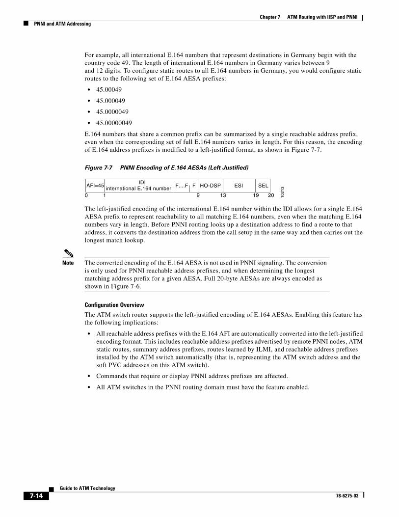
Chapter 7 ATM Routing with IISP and PNNIPNNI and ATM Addressing
For example, all international E.164 numbers that represent destinations in Germany begin with the country code 49. The length of international E.164 numbers in Germany varies between 9 and 12 digits. To configure static routes to all E.164 numbers in Germany, you would configure static routes to the following set of E.164 AESA prefixes:
• 45.00049
• 45.000049
• 45.0000049
• 45.00000049
E.164 numbers that share a common prefix can be summarized by a single reachable address prefix, even when the corresponding set of full E.164 numbers varies in length. For this reason, the encoding of E.164 address prefixes is modified to a left-justified format, as shown in Figure 7-7.
Figure 7-7 PNNI Encoding of E.164 AESAs (Left Justified)
The left-justified encoding of the international E.164 number within the IDI allows for a single E.164 AESA prefix to represent reachability to all matching E.164 numbers, even when the matching E.164 numbers vary in length. Before PNNI routing looks up a destination address to find a route to that address, it converts the destination address from the call setup in the same way and then carries out the longest match lookup.
Note The converted encoding of the E.164 AESA is not used in PNNI signaling. The conversion is only used for PNNI reachable address prefixes, and when determining the longest matching address prefix for a given AESA. Full 20-byte AESAs are always encoded as shown in Figure 7-6.
Configuration Overview
The ATM switch router supports the left-justified encoding of E.164 AESAs. Enabling this feature has the following implications:
• All reachable address prefixes with the E.164 AFI are automatically converted into the left-justified encoding format. This includes reachable address prefixes advertised by remote PNNI nodes, ATM static routes, summary address prefixes, routes learned by ILMI, and reachable address prefixes installed by the ATM switch automatically (that is, representing the ATM switch address and the soft PVC addresses on this ATM switch).
• Commands that require or display PNNI address prefixes are affected.
• All ATM switches in the PNNI routing domain must have the feature enabled.
international E.164 number FF....F SELAFI=45IDI
ESIHO-DSP
1021
3
10 9 13 19 20
7-14Guide to ATM Technology
78-6275-03

Chapter 7 ATM Routing with IISP and PNNIPNNI and ATM Addressing
Designing an ATM Address Plan—Hierarchical PNNIYour ATM address plan is key to efficient operation and management of PNNI networks. When designing an ATM address plan, the three most important things to remember are:
• Your ATM address prefixes must be globally unique.
• The addresses must be hierarchical, corresponding to your network topology.
• You must plan for future network expansion.
Globally Unique ATM Address Prefixes
To create private ATM networks that can interoperate with a global ATM internetwork, all ATM addresses should be globally unique. For scalability reasons, we also recommend that addresses align with the network topology.
You can obtain globally unique address prefixes from a national or world registration authority or they can be suballocated to you from a service provider’s address space. See the section “Obtaining Registered ATM Addresses” section on page 2-17 for information on obtaining and registering ATM addresses. Make sure that the addresses you assign in your network are derived from a globally unique address prefix, as shown in Figure 7-8.
Figure 7-8 Unique ATM Address Prefix Used to Assign ATM Addresses
Hierarchical Addresses
The high order domain-specific part (HO-DSP) remainder, the part of the address between the assigned ATM address prefix and the ESI, should be assigned in a hierarchical manner. All systems in the network share the assigned ATM address prefix. The assigned address space can be further subdivided by providing longer prefixes to different regions of the network. Within each peer group, the first level bits of each ATM switch address should match the corresponding bits of the Peer Group Identifier (PGI) value. An example of a hierarchical address assignment is shown in Figure 7-9.
1013
5
Octet
Assigned ATM Addr prefix HO-DSP remainder ESI Sel
0 13 2019
7-15Guide to ATM Technology
78-6275-03

Chapter 7 ATM Routing with IISP and PNNIPNNI and ATM Addressing
Figure 7-9 Example Hierarchical Address Assignment
Note that the address prefix is longer at each lower level of the PNNI hierarchy shown in Figure 7-9.
The advantages of hierarchical address assignment include:
• Greatly increased scalability by minimizing the number of PNNI routes stored and processed by each node
• Simplified configuration and management of the PNNI hierarchy
When the ATM network topology (which consists of switches, links, and virtual path [VP] tunnels) differs from the logical topology (which consists of VPNs and virtual LANs), it is important that the address hierarchy follow the network topology. You can construct the logical topology using other features, such as emulated LANs or Closed User Groups (CUGs).
Planning for Future Growth
When constructing the address hierarchy, it is important to plan ahead for the maximum number of levels that you might need for future growth. Not all levels in the addressing hierarchy need to be used by PNNI. It is possible to run with fewer PNNI levels in the beginning, and then migrate to more levels of hierarchy in the future. For example, you can configure the network as one large peer group where the PGI value is based on the assigned ATM address prefix. By planning ahead, you can easily migrate to more levels of hierarchy without manually renumbering all of the switches and end systems.
You can subdivide the HO-DSP remainder to allow for upward and downward future growth. For example, assume that you have 6 octets available for the HO-DSP remainder: 8 through 13 (as shown in Figure 7-10).
Figure 7-10 HO-DSP Remainder Subdivision Example
Corporate peer groupassigned ATM address prefix
47.0091.4455.6677
Level 56
Level 64
Level 72
San Francisco47.0091.4455.6677.22
San FranciscoBuilding A
47.0091.4455.6677.2233
New York47.0091.4455.6677.11
New YorkBuilding B
47.0091.4455.6677.1144
1015
5
1013
4
Octet
Level
HO-DSP remainder
56 64 72 80 88 96 104
8 9 10 11 12 13
7-16Guide to ATM Technology
78-6275-03

Chapter 7 ATM Routing with IISP and PNNIPNNI and ATM Addressing
The HO-DSP remainder in this example spans levels 56 through 104. To allow for future expansion at the lowest level of the hierarchy, you must provide sufficient addressing space in the HO-DSP remainder to accommodate all future switches. Assume that you start with the lowest level at 88. For administrative purposes, in the future you might want to group some of these switches into peer groups where additional switches can be added. For those switches that will be part of the new peer group you should assign addresses that can be easily clustered into a level 96 peer group. These addresses would share a common 12th octet, leaving the 13th octet for downward future expansion. The octet pairs (12 and 13) for these switches could be as follows: (01, 00), (02, 00), (03, 00) and so on, while switches that will be added in the future could be: (02, 01), (02, 02), (02, 03) and so on.
This type of addressing scheme leaves room for expansion without requiring address modification. If you add a hierarchical level 96, the switches form a new peer group at level 96. Although you started with no more than 256 switches at the lowest level, by expanding this to two levels in the future, you can accommodate up to 65,536 switches in the same region. An example of HO-DSP assignment is shown in Figure 7-11.
Figure 7-11 Example of HO-DSP Assignment for Future Expansion
Following similar guidelines, you can plan for future expansion in the upward and downward direction. Specifically, you can expand upward by adding hierarchical levels as your network grows in size.
10
13
3
Values for the 6 octets HO-DSP remainder
0100.0100.0202
Future expansion
Future expansion
Future peer group
0100.0100.0200
0100.0100.0300
0100.0100.0101
0100.0100.0100
0100.0100
0100.0200
7-17Guide to ATM Technology
78-6275-03

Chapter 7 ATM Routing with IISP and PNNIPNNI Configuration
PNNI ConfigurationThis section describes the configuration of a flat PNNI network and provides an overview of the tasks involved.
PNNI Without HierarchyIf your needs do not include current or future support for a hierarchical topology and you do not plan to connect to a service provider network, you do not need to perform any manual PNNI configuration on your ATM switch router. The default ATM address allows your ATM switch router to be preconfigured as a single lowest-level PNNI node (locally identified as node 1) with a level of 56. The node ID and peer group ID are calculated based on the current active ATM address.
Lowest Level of the PNNI HierarchyThis section provides an overview of configuring the lowest level in a PNNI hierarchy. When only the lowest-level nodes are configured, there is no hierarchical structure. You would configure the lowest level for the following reasons:
• To reconfigure the address to connect to a service provider network
• To prepare for higher levels to be added in the hierarchy
To configure a lowest level of the PNNI hierarchy requires the following steps:
Step 1 Configure an ATM address and PNNI node level
Step 2 Configure static routes
Step 3 Configure a summary address
Step 4 Configure scope mapping
These tasks are described in the following sections.
ATM Address and PNNI Node Level
The default PNNI configuration of the ATM switch router is a node at level 56. To configure a node in a higher level of the PNNI hierarchy, the value of the node level must be a smaller number. For example, a three-level hierarchical network could progress from level 72 to level 64 to level 56. Notice that the level numbers graduate from largest at the lowest level (72) to smallest at the highest level (56). (See Figure 7-9 earlier in this chapter.)
7-18Guide to ATM Technology
78-6275-03

Chapter 7 ATM Routing with IISP and PNNIPNNI Configuration
Configuration Overview
To change the active ATM address and (optionally) change the node level requires the following steps:
Step 1 In global configuration mode, configure a new ATM address on the ATM switch router.
Step 2 Display the new ATM address to verify it.
Step 3 Remove the old ATM address.
Step 4 In ATM router configuration mode, disable the PNNI node.
Step 5 Reenable the PNNI node and, if necessary, specify a new node level.
Disabling then reenabling the node recalculates the node IDs and peer group IDs.
Static Routes with PNNI
Because PNNI is a dynamic routing protocol, static routes are not necessary between nodes that support PNNI. However, you can extend the routing capability of PNNI beyond nodes that support PNNI to:
• Connect to nodes outside of a peer group that do not support PNNI
• Define routes to end systems that do not support ILMI
Note Two PNNI peer groups can be connected using the IISP protocol. Connecting PNNI peer groups requires that a static route be configured on the IISP interfaces, allowing connections to be set up across the IISP link(s).
Configuration Overview
Configuring a static route requires the following steps:
Step 1 In interface configuration mode, configure the interface as IISP.
This procedure is described in the “IISP Interfaces” section on page 3-5.
Step 2 Configure a static route to a reachable address prefix.
A static route on an interface allows all ATM addresses matching the configured address prefix to be reached through that interface.
Summary Addresses
Configuring summary addresses reduces the amount of information advertised by a PNNI node and contributes to scalability in large networks. Each summary address consists of a single reachable address prefix that represents a collection of end system or node addresses.
We recommend that you use summary addresses when all end system addresses that match the summary address are directly reachable from the node. If an end system that matches the summary address is not directly reachable from the node, it can still be reached assuming that the advertised prefix is longer than the summary address. This is because PNNI always selects the nodes advertising the longest matching prefix to a destination address.
7-19Guide to ATM Technology
78-6275-03

Chapter 7 ATM Routing with IISP and PNNIPNNI Configuration
By default, each lowest-level node has a summary address equal to the 13-byte address prefix of the ATM address of the switch. This address prefix is advertised into its peer group.
Note Summary addresses less than 13 bytes long must not be used with autoconfigured ATM addresses, since other switches with autoconfigured ATM addresses matching the summary can exist outside of the default PNNI peer group.
Configuration Overview
If all nodes and end systems in your PNNI network are running ILMI, you do not need to configure reachable addresses to establish calls between end systems. If, however you do not run ILMI you might need to configure reachable addresses; for example, when you have an address you need to reach over an IISP connection.
Summary addresses, other than the default, must be configured on each node. Each node can have multiple summary address prefixes. Configuring summary address prefixes requires the following steps:
Step 1 In ATM router configuration mode, remove the default summary address.
Perform this step when system that match the first 13 bytes of the ATM address(es) of the node are attached to different ATM switch routers. You might also want to use this for security purposes.
Step 2 Select the node by its node index and disable autosummarization.
Step 3 Configure the ATM PNNI summary address prefix.
Scope Mapping
The PNNI address scope allows you to restrict advertised reachability information within configurable boundaries.
Note On UNI and IISP interfaces, the scope is specified in terms of organizational scope values ranging from 1 (local) to 15 (global). (Refer to the ATM Forum UNI Signaling 4.0 specification for more information.)
In PNNI networks, the scope is specified in terms of PNNI levels. The mapping from organizational scope values used at UNI and IISP interfaces to PNNI levels is configured on the lowest-level node. The mapping can be determined automatically (which is the default setting) or manually, depending on the configuration of the scope mode.
In manual mode, whenever the level of node 1 is modified, the scope map should be reconfigured to avoid unintended suppression of reachability advertisements. Misconfiguration of the scope map might cause addresses to remain unadvertised.
In automatic mode, the UNI to PNNI level mapping is automatically reconfigured whenever the level of the node 1 is modified. The automatic reconfiguration avoids misconfigurations caused by node level modifications. Automatic adjustment of scope mapping uses the values shown in Table 7-1.
7-20Guide to ATM Technology
78-6275-03
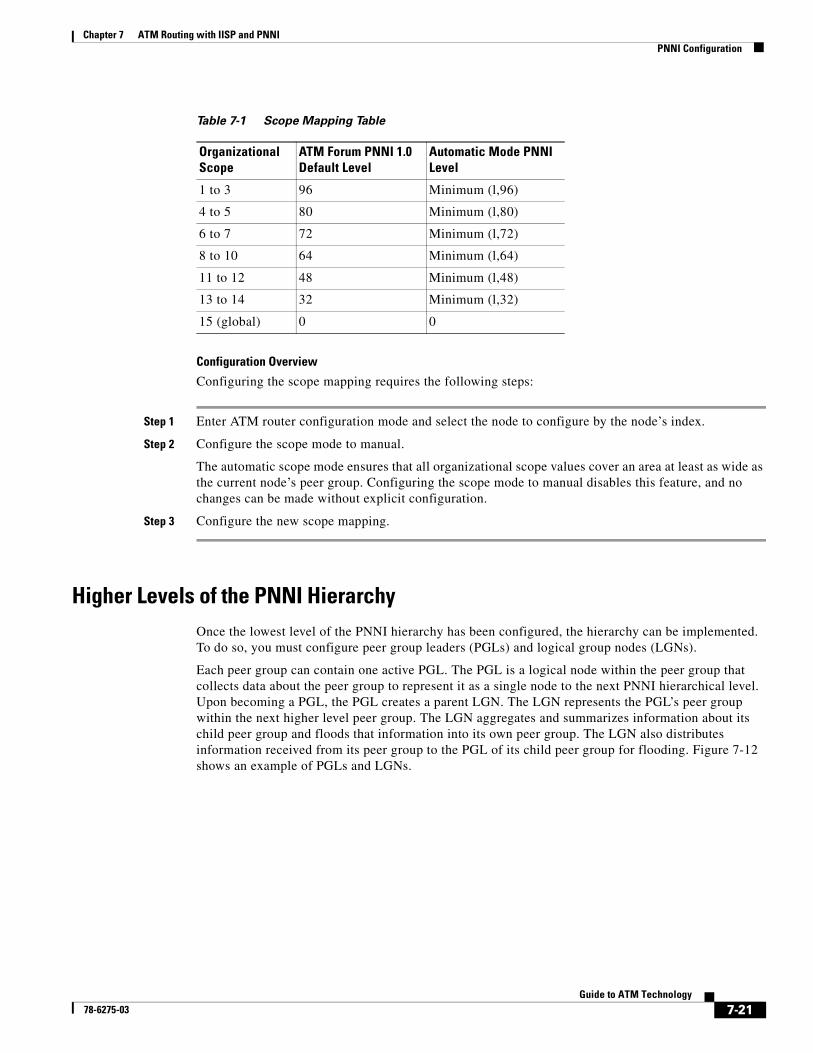
Chapter 7 ATM Routing with IISP and PNNIPNNI Configuration
Configuration Overview
Configuring the scope mapping requires the following steps:
Step 1 Enter ATM router configuration mode and select the node to configure by the node’s index.
Step 2 Configure the scope mode to manual.
The automatic scope mode ensures that all organizational scope values cover an area at least as wide as the current node’s peer group. Configuring the scope mode to manual disables this feature, and no changes can be made without explicit configuration.
Step 3 Configure the new scope mapping.
Higher Levels of the PNNI HierarchyOnce the lowest level of the PNNI hierarchy has been configured, the hierarchy can be implemented. To do so, you must configure peer group leaders (PGLs) and logical group nodes (LGNs).
Each peer group can contain one active PGL. The PGL is a logical node within the peer group that collects data about the peer group to represent it as a single node to the next PNNI hierarchical level. Upon becoming a PGL, the PGL creates a parent LGN. The LGN represents the PGL’s peer group within the next higher level peer group. The LGN aggregates and summarizes information about its child peer group and floods that information into its own peer group. The LGN also distributes information received from its peer group to the PGL of its child peer group for flooding. Figure 7-12 shows an example of PGLs and LGNs.
Table 7-1 Scope Mapping Table
Organizational Scope
ATM Forum PNNI 1.0Default Level
Automatic Mode PNNILevel
1 to 3 96 Minimum (l,96)
4 to 5 80 Minimum (l,80)
6 to 7 72 Minimum (l,72)
8 to 10 64 Minimum (l,64)
11 to 12 48 Minimum (l,48)
13 to 14 32 Minimum (l,32)
15 (global) 0 0
7-21Guide to ATM Technology
78-6275-03

Chapter 7 ATM Routing with IISP and PNNIPNNI Configuration
Figure 7-12 PGLs and LGNs
Implementation Considerations
When creating the PNNI hierarchy, keep in mind the following guidelines:
• You should select switches that are eligible to become PGLs at each level of the hierarchy.
Nodes can become PGLs through the peer group leader election process. Each node has a configured election priority. To be eligible for election, the configured priority must be greater than zero and a parent node must be configured. Normally the node with the highest configured leadership priority in a peer group is elected PGL.
• You can configure multiple nodes in a peer group as eligible PGLs.
By configuring multiple nodes in a peer group with a nonzero leadership priority, if one PGL becomes unreachable, the node configured with the next highest election leadership priority becomes the new PGL.
Note The choice of PGL does not directly affect the selection of routes across a peer group.
• Because any one peer group can consist of both lowest level nodes and LGNs, lowest level nodes should be preferred as PGLs.
Configuring the network hierarchy with multiple LGNs at the same switch creates additional PNNI processing and results in slower recovery from failures. Selecting switches for election with more processing capability (for example, because of a smaller volume of call processing compared to others) might be better.
• We recommend that every node in a peer group that can become a PGL have the same parent node configuration.
• Peer group nodes must be connected in such a way that the (single-hop or multi-hop) path to any other peer group member lies entirely within the peer group.
Ideally there should be multiple independent paths between any two peer nodes, so that if any single link or node fails, the peer group is not partitioned into two nonconnected groups of nodes.
• Paths between any two border nodes within the peer group should ideally have no more hops than paths lying outside of the peer group that might connect those same nodes together.
Peergroup
1
Peergroup
1.1
Peergroup
1.2
Peergroup
1.3
Logical group node
Peer group leader
S69
02
1.1
1.21.3
1.1.2
1.1.1
1.1.3 1.2.41.2.3
1.2.1 1.3.11.3.2
1.3.3
1.3.41.3.5
1.2.2
7-22Guide to ATM Technology
78-6275-03
Chapter 7 ATM Routing with IISP and PNNIPNNI Configuration
• If there are multiple border nodes that connect to the same neighboring peer group, it is preferable to minimize the number of hops between them.
• Some peer group topologies, especially those with large numbers of nodes, might benefit from using complex node representation (see the “Complex Node Representation for LGNs” section on page 7-35).
Configuration Overview
Configuring the higher levels of the PNNI hierarchy requires the following steps:
Step 1 Configure an LGN and peer group identifier.
Step 2 Configure the node name.
Step 3 Configure a parent node.
Step 4 Configure the node election leadership priority.
Step 5 Configure a summary address.
These tasks are described in the following sections.
LGN and Peer Group Identifier
The LGN is created only when the child node in the same switch (that is, the node whose parent configuration points to this node) is elected PGL of the child peer group.
Higher level nodes only become active if:
• A lower-level node specifies the higher-level node as a parent.
• The election leadership priority of the child node is configured with a nonzero value, and the node is elected as the PGL.
Configuration Overview
Configuring an LGN and peer group identifier requires the following steps:
Step 1 Enter ATM router configuration mode.
Step 2 Configure the logical node with the node index, level, and, optionally, peer group identifier.
The peer group identifier defaults to a value created from the first part of the child peer group identifier, and does not need to be specified. If you want a non-default peer group identifier, you must configure all logical nodes within a peer group with the same peer group identifier.
Step 3 If you have more than one logical node on the same switch, specify a different node index to distinguish it.
7-23Guide to ATM Technology
78-6275-03

Chapter 7 ATM Routing with IISP and PNNIPNNI Configuration
Node Name
The PNNI node name for a lowest level node defaults to the host name. The node name for a parent node defaults to the hostname with a suffix that represents the node index and level.
If you prefer higher level node names that more accurately reflect the child peer group, you can assign a new name to a node at any level. For example, you could change the parent node name to Calif1 to represent the entire geographic region of the peer group to which it belongs.
Configuration Overview
Configuring a new node name requires the following steps:
Step 1 Enter ATM router configuration mode and specify the node to configure by the node’s index.
Step 2 Specify the new name.
We recommend you choose a node name of 12 characters or less so that your screen displays remain nicely formatted and easy to read.
After a node name has been configured, it is distributed to all other nodes by PNNI flooding.
Parent Node Designation
For a node to be eligible to become a PGL within its own peer group, it must have a configured parent node and nonzero election leadership level (described in the next section, “Node Election Leadership Priority”). If the node is elected a PGL, the node specified as the parent becomes the parent node and represents the peer group at the next hierarchical level.
Configuration Overview
Configuring a parent node requires the following steps:
Step 1 Enter ATM router configuration mode and select the node to configure using the node’s index.
Step 2 Specify a node index for the parent.
You must use a node index higher than the index of the child node.
Node Election Leadership Priority
Normally the node with the highest election leadership priority is elected PGL. If two nodes share the same election priority, the node with the highest node identifier becomes the PGL. To be eligible for election, the configured priority must be greater than zero. You can configure multiple nodes in a peer group with nonzero leadership priority so that if one PGL becomes unreachable, the node configured with the next highest election leadership priority becomes the new PGL.
Note The choice of PGL does not directly affect the selection of routes across the peer group.
7-24Guide to ATM Technology
78-6275-03

Chapter 7 ATM Routing with IISP and PNNIPNNI Configuration
The control for election is done through the assignment of leadership priorities. We recommend that the leadership priority space be divided into three tiers:
• First tier: 1 to 49
• Second tier: 100 to 149
• Third tier: 200 to 205
This subdivision is used because when a node becomes PGL, it increases the advertised leadership priority by a value of 50. This avoids instabilities after election.
Configuration Overview
Configuring the node election leadership priority requires the following steps:
Step 1 Enter ATM router configuration mode and select the node to configure using the node’s index.
Step 2 Assign the node an election leadership priority number.
The following guidelines apply:
• Nodes that you do not want to become PGLs should remain with the default leadership priority value of 0.
• Unless you want to force one of the PGL candidates to be the PGL, you should assign all leadership priority values within the first tier. After a node is elected PGL, it remains PGL until it goes down or is configured to step down.
• If certain nodes should take precedence over nodes in the first tier, even if one is already PGL, leadership priority values can be assigned from the second tier. We recommend that you configure more than one node with a leadership priority value from this tier. This prevents one unstable node with a larger leadership priority value from repeatedly destabilizing the peer group.
• If you need a strict master leader, use the third tier.
Summary Addresses
Summary addresses can be used to decrease the amount of information advertised by a PNNI node, and thereby contribute to scaling in large networks. Each summary address consists of a single reachable address prefix that represents a collection of end system or node addresses that begin with the given prefix.
We recommend that you use summary addresses when all end system addresses that match the summary address are directly reachable from the node. If an end system that matches the summary address is not directly reachable from the node, it can still be reached assuming that the advertised prefix is longer than the summary address. This is because PNNI always selects the nodes advertising the longest matching prefix to a destination address.
A single default summary address is configured for each LGN in the PNNI hierarchy. The length of that summary for any LGN equals the level of the child peer group, and its value is equal to the first level bits of the child peer group identifier. This address prefix is advertised into the LGN’s peer group. For example, switch A has two PNNI nodes running on it:
• Node 1, level 96 (lowest)
• Node 2, level 56
7-25Guide to ATM Technology
78-6275-03

Chapter 7 ATM Routing with IISP and PNNIAdvanced PNNI Features
The switch ATM address is 47.0091.4455.6677.1144.1017.3333.0060.3e7b.3a01.00. The summary address prefix of the LGN (node 2) is 47.0091.4455.6677.1144.1017.33; that is, the first 96 bits of the node 1 address.
Summary addresses other than defaults must be explicitly configured on each node. A node can have multiple summary address prefixes. Note that every node in a peer group that has a potential to become a PGL should have the same summary address lists in its parent node configuration.
Configuration Overview
Configuring the nondefault summary address requires the following steps:
Step 1 Enter ATM router configuration mode and select the node to configure by the node’s index.
Step 2 Disable autosummarization.
Step 3 Configure the new summary address prefix.
Advanced PNNI FeaturesThis section describes advanced PNNI features that allow you to fine-tune the performance of your PNNI network. These features include adjusting parameters that affect route selection, parameters that are used in calculating topology attributes, and parameters that are used by the protocol to manage and distribute information.
Tuning Route SelectionThis section describes features you can use to tune the mechanisms by which routes are selected in your PNNI network.
Background Route Computation
The ATM switch router supports the following two route selection modes that are appropriate for different needs:
• On-demand—A separate route computation is performed each time a SETUP or ADD PARTY message is received over a UNI or IISP interface. In this mode, the most recent topology information received by this node is always used for each setup request.
• Background routes—Call setups are routed using precomputed routing trees. In this mode, multiple background trees are precomputed for several service categories and QoS metrics. When a call is placed from point A to point B, PNNI chooses a cached route from the background route table instead of computing a route on demand. This scenario eases the load on the CPU and provides for a faster rate of processing the call setups. If no route can be found in the multiple background trees that satisfies the QoS requirements of a particular call, route selection reverts to on-demand route computation.
The background routes mode should be enabled in large networks where it usually exhibits less-stringent processing requirements and better scalability. Route computation is performed at almost every poll interval when a significant change in the topology of the network is reported or when
7-26Guide to ATM Technology
78-6275-03

Chapter 7 ATM Routing with IISP and PNNIAdvanced PNNI Features
significant threshold changes have occurred since the last route computation. It is most effective in networks where the topology with respect to QoS is relatively stable. Campus LANE networks can use this feature very effectively, since all the SVCs in the network belong to the UBR or ABR category.
Configuration Overview
Enabling background route computation requires the following steps:
Step 1 Enter ATM router configuration mode.
Step 2 Enable background route computation.
You can specify a threshold for the number of insignificant changes necessary to trigger a new computation. You can also specify a poll interval for detecting the changes that trigger recomputation.
Parallel Links, Link Selection, and Alternate Links
Link selection applies to parallel PNNI links between two switches. Link selection allows you to choose the method the switch uses during call setup for selecting one link among multiple parallel links to forward the call.
Note Calls always use the load balance method over parallel IISP links between two switches.
Table 7-2 lists the PNNI link selection methods from which you can choose.
The switch applies a single link selection method for a group of parallel links connected to a neighbor switch. If multiple links within this group are configured with a different link selection method, then the switch selects a method according to the order of precedence as shown in Table 7-2. For example, if any link within the parallel link group is configured as admin-weight-minimize, then admin-weight-minimize becomes the link selection method for the entire group. Further, the admin-weight-minimize, blocking-minimize, and transmit-speed-maximize methods are only available to guaranteed service categories (CBR, VBR-NRT, and VBR-RT) with the default set at blocking-minimize. Best effort traffic (ABR and UBR) is always load balanced by default.
Table 7-2 PNNI Link Selection Methods
PrecedenceOrder Method Description
Service CategoryAvailability
1 admin-weight-minimize Place the call on the link with the lowest administrative weight.
CBR, VBR-RT, VBR-NRT
2 blocking-minimize Place the call on the link so that higher bandwidth is available for subsequent calls, thus minimizing call blocking.
CBR, VBR-RT, VBR-NRT
3 transmit-speed-maximize Place the call on the highest speed link.
CBR, VBR-RT, VBR-NRT
4 load-balance Place the call on the link so that the load is balanced among parallel links for a group.
ABR, UBR
7-27Guide to ATM Technology
78-6275-03

Chapter 7 ATM Routing with IISP and PNNIAdvanced PNNI Features
You can also specify one or more links among the parallel links as an alternate (or backup) link. An alternate link is a link that is used only when all other non-alternate links are either down or full. Alternate links are not considered part of the parallel link group targeted for link selection. By default, calls are always load balanced over multiple parallel alternate links.
Configuration Overview
Link selection is configured on a per-interface basis. To configure link selection, take the following steps:
Step 1 Determine the interface that terminates one of a group of parallel links, and enter interface configuration mode.
Step 2 Configure the link selection method and specify the traffic category. Additionally, you can specify an alternate link on an interface.
Maximum Administrative Weight Percentage
In an ATM network that runs at high utilization rates, finding a path that satisfies the requested QoS can lead to paths with a much higher administrative weight compared to the shortest path without QoS constraints. The maximum administrative weight percentage feature is useful when the best path violates constraints and an alternate path must be chosen. By using this feature you can prevent the selection of alternate routes that consume too many network resources.
Administrative weight is a cumulative metric and provides a measure similar to hop count. The maximum administrative weight percentage feature thus provides a generalized form of a hop count limit. The maximum acceptable administrative weight is equal to the specified percentage of the least administrative weight of any route to the destination (from the background routing tables). For example, if the least administrative weight to the destination is 5040 and the configured percentage is 300, the maximum acceptable administrative weight for the call is 5040 * 300 / 100, or 15120.
Configuration Overview
The maximum administrative weight percentage feature is disabled by default on the ATM switch router. The feature, when enabled, only takes effect if background route computation is also enabled.
Configuring the maximum administrative weight percentage requires the following steps:
Step 1 Enter ATM router configuration mode.
Step 2 Specify the maximum administrative weight percentage. You configure the maximum administrative weight percentage with a value from 100 to 2000.
Precedence of Reachable Addresses
The route selection algorithm chooses routes to particular destinations using the longest match reachable address prefixes known to the switch. When there are multiple longest match reachable address prefixes known to the switch, the route selection algorithm first attempts to find routes to reachable addresses with types of greatest precedence. Among multiple longest match reachable address prefixes of the same type, routes with the least total administrative weight are chosen first.
7-28Guide to ATM Technology
78-6275-03

Chapter 7 ATM Routing with IISP and PNNIAdvanced PNNI Features
Reachable addresses fall into the following categories:
• PNNI (learned) or static (IISP)
• Local (directly attached to the switch) or remote (attached to another switch)
• Internal (belonging to the network) or remote (belonging to an attached network)
Local internal reachable addresses, whether learned via ILMI or as static routes, are given highest precedence or a precedence value of one. The other reachable address types have default values of 2 through 4; you can modify these values through manual configuration.
Configuration Overview
Configuring the reachable address precedence requires the following steps:
Step 1 Enter ATM router configuration mode.
Step 2 Specify the reachable address type and a precedence value.
When you configure the precedence for reachable address types, you are modifying the default values used by the ATM switch router. Refer to your ATM switch router software documentation for the default values of each reachable address type.
Manually Configured Explicit Paths
Normally soft PVCs are automatically routed by PNNI over paths that meet the traffic parameter objectives. However, there might be some cases where manually configured paths are desirable.
The explicit path feature enables you to manually configure either a fully specified or partially specified path for routing soft permanent virtual channel connections (soft PVCCs) and soft permanent virtual path connections (soft PVPCs). Once these routes are configured, up to three explicit paths can be applied to these connections.
A fully specified path includes all adjacent nodes (and optionally the corresponding exit port) for all segments of the path. A partially specified path consists of one or more segment target nodes that should appear in their proper order in the explicit path. The standard routing algorithm is used to determine all unspecified parts of the partially specified path.
Configuration Overview
Step 1 Enter PNNI explicit path configuration mode.
Step 2 Add entries to the explicit path. You can add three types of entries:
a. Next-node—specifies the next adjacent node for fully specified paths.
b. Segment-target—specifies the target node for cases where the path through intermediate nodes should be automatically routed.
c. Exclude-node—specifies nodes or ports that are excluded from all partial path segments.
You can also edit an explicit path after configuring it, or modify an explicit path while it is in use; see the “Soft PVCs with Explicit Paths” section on page 4-10. For detailed information on configuring and editing explicit paths, refer to the ATM switch router software documentation.
7-29Guide to ATM Technology
78-6275-03
Chapter 7 ATM Routing with IISP and PNNIAdvanced PNNI Features
Tuning Topology AttributesThis section describes features you can use to tune the topology attributes of your PNNI network.
Administrative Weight—Global Mode and Per-Interface Values
Administrative weight is the primary routing metric for minimizing use of network resources. Administrative weight can be assigned globally to all links in one of two modes, uniform or linespeed. Uniform mode assigns the same administrative weight to every link; linespeed mode assigns an administrative weight based on the maximum cell rate (MCR) of the interface. Administrative weight can also be assigned on a per-interface basis with a specific numeric value.
In the absence of other constraints, configuring the administrative weight as uniform causes PNNI routing to minimize the number of hops. Basing administrative weight on linespeed allows path selection to prefer paths along higher bandwidth interfaces. This happens because in linespeed mode higher speed links have lower administrative weights, and are thus preferred during route selection. Figure 7-13 provides an example of how network administrative weight works.
The network depicted at the top of Figure 7-13 is configured as uniform, causing equal administrative weight to be assigned to each link. The identical network at the bottom of the figure is configured as linespeed. The links between SW1 and SW2 (SW1p1 to SW2p1) and SW2 and SW3 (SW2p2 to SW3p2) are both faster OC-12 connections and therefore have lower administrative weights. PNNI interprets the route over the two OC-12 links as being administratively equivalent to a more direct route between SW1 and SW3 using the OC-3 connection.
7-30Guide to ATM Technology
78-6275-03

Chapter 7 ATM Routing with IISP and PNNIAdvanced PNNI Features
Figure 7-13 Network Administrative Weight Example
Configuration Overview
When you assign the global administrative weight mode, you are doing so for all links attached to the node. Configuring the global administrative weight mode requires the following steps:
Step 1 Enter global configuration mode.
Step 2 Specify the administrative weight mode as uniform or linespeed.
With uniform mode, every link has a default value of 5040. With linespeed, the value of administrative weight is assigned a value inversely proportional to the speed of the interface.
5040 5040
5040SW 1
SW 2
SW 3
ESsource UNI UNI
OC-3 connection
Administrative Weight Configured Uniform
OC-12 connection OC-12 connection
32
21
1 2
ESdestination
2520 2520
5040SW 1
SW 2
SW 3
S49
04
ESsource UNI UNI
OC-3 connection
= Administrative weight
Administrative Weight Configured Linespeed
OC-12 connection OC-12 connection
32
21
1 2
ESdestination
7-31Guide to ATM Technology
78-6275-03

Chapter 7 ATM Routing with IISP and PNNIAdvanced PNNI Features
Configuring a specific administrative weight on an interface requires the following steps:
Step 1 Select the interface you want to configure and enter interface configuration mode.
Step 2 Specify an administrative weight value and, optionally, a service category.
When you specify a service category, you limit the use of this value to calls requesting that service category.
Transit Call Restriction
Transit calls are calls that originate from another ATM switch and pass through the ATM switch router. Under some conditions you might want to eliminate this transit traffic on edge devices and only allow traffic originating or terminating at the ATM switch router.
Configuration Overview
The following steps are required to block transit calls on a node:
Step 1 Enter ATM router configuration mode and select the node using the node’s index.
Step 2 Enable transit restriction.
Route Redistribution
Redistribution instructs PNNI to distribute reachability information from non-PNNI sources throughout the PNNI routing domain. The ATM switch router supports redistribution of static routes, such as those configured on IISP interfaces.
Configuration Overview
The route redistribution feature is enabled by default on the ATM switch router. Disabling the feature requires the following steps:
Step 1 Enter ATM router configuration mode and select the node using the node index.
Step 2 Disable static route redistribution.
Aggregation Tokens
One of the tasks performed by the LGN is link aggregation. To describe the link aggregation algorithms, we need to introduce the terms of upnodes, uplinks and aggregated links. An uplink is a link to a higher level node, called an upnode. The term higher means at a higher level in the hierarchy compared to the level of our peer group. The aggregation token controls the grouping of multiple physical links into logical links. Uplinks to the same upnode, with the same aggregation token value, are represented at a higher level as horizontal aggregated links. Resource Availability Information Groups (RAIGs) are computed according to the aggregation algorithm.
7-32Guide to ATM Technology
78-6275-03

Chapter 7 ATM Routing with IISP and PNNIAdvanced PNNI Features
Figure 7-14 shows four physical links between four nodes in the two lower-level peer groups. Two physical links between two nodes in different peer groups are assigned the PNNI aggregation token value of 221; the other two are assigned the value of 100. These four links are summarized and represented as two links in the next higher PNNI level.
Figure 7-14 PNNI Aggregation Token
Configuration Overview
Configuring the aggregation token requires the following steps:
Step 1 Select the interface on which you want to configure the aggregation token and enter interface configuration mode.
Step 2 Assign an aggregation token value.
The following guidelines apply when configuring the PNNI aggregation token:
• You only need to configure the interface on one side of the link. If the configured aggregation token value of one side is zero and the other side is nonzero, the nonzero value is used by both sides as the aggregation token value.
• If you choose to configure an aggregation token value on both interfaces, make sure the aggregation token values match. If the values do not match, the configuration is invalid and the default aggregation token value of zero is used.
• If the metrics for uplinks with the same aggregation token differ widely from each other, no single set of metrics can accurately represent them at the LGN level. When you assign separate aggregation tokens to some of the uplinks, they are treated as separate higher level horizontal links that more accurately represent their metrics.
Aggregation Mode
In the PNNI hierarchy, link aggregation is used to represent several parallel links between two peer groups as a single higher-level link, as shown in Figure 7-14. The ATM switch router has two algorithms, best link and aggressive, which control how the metrics for the higher level links are derived from the individual parallel links that have the same aggregation token. The aggregation mode can be assigned for links or for nodes with complex node representation (see the “Complex Node Representation for LGNs” section on page 7-35).
221
221
221
100
100
100
S69
28
Peer group 1
Peer group 1.2
Peer group 1.1
7-33Guide to ATM Technology
78-6275-03

Chapter 7 ATM Routing with IISP and PNNIAdvanced PNNI Features
Best Link Aggregation Mode
When specified for links, best link selects the best values for each individual metric from all links or paths that are being aggregated. In this mode, there might be no single lower-level link that is as good as the higher-level link for all of the metrics.
When specified for complex nodes, best link selects the parameters from a single path even when multiple paths exist between the border nodes. The best path for each service category is chosen based on a single metric considered most important for the service category.
Aggressive Aggregation Mode
When specified for links, aggressive aggregation mode causes one of the lower-level links to be chosen as the best link based on one or two metrics. All metrics from the selected lower-level link are copied to the higher-level aggregated link. In this mode, there is at least one lower-level link with metrics matching the higher-level link.
When specified for complex nodes, the aggressive mode selects the best parameters from among multiple paths joining a pair of border nodes. The resulting path metrics might look better than any single real path between the border nodes. This mode can make it more likely that connections will be routed through the complex LGN.
Configuration Overview
Configuring the aggregation mode requires the following steps:
Step 1 Enter ATM router configuration mode and select the node to configure using the node’s index.
Step 2 Specify link or node, the service category, and aggregation mode. The metrics for the specified service category are aggregated using the mode you select.
Significant Change Thresholds
PTSEs would overwhelm the network if they were transmitted every time any parameter in the network changed. To avoid this problem, PNNI uses significant change threshold parameters, which define the level of change in metrics that triggers PNNI to update and send PTSEs. The significant change threshold parameters apply to all PTSE types that include metrics.
Note Any change in administrative weight or CLR is considered significant and triggers a new PTSE.
Configuration Overview
The ATM switch router uses default values to determine when to trigger PTSEs. When you configure the significant change threshold parameters, you are specifying a value, expressed as a minimum threshold percent or proportional multiplier, that defines when a change is significant. Available cell rate (AvCR), cell delay variation (CDV), and cell transfer delay (CTD) can be configured.
7-34Guide to ATM Technology
78-6275-03

Chapter 7 ATM Routing with IISP and PNNIAdvanced PNNI Features
Configuring the significant change threshold requires the following steps:
Step 1 Enter ATM router configuration mode and select the node to configure using the node’s index.
Step 2 Specify the metric and percent of change.
You can configure additional parameters that affect the timing and frequency of Hello and PTSE exchanges, as described in the “PNNI Hello, Database Synchronization, and Flooding Parameters” section on page 7-39.
Complex Node Representation for LGNsBy default, higher-level LGNs represent their child peer groups in the simple node representation. With simple node representation, the entire PG is represented as a single node. When there are many nodes in the child PG, you can use complex node representation to present a more accurate model of the PG.
Limitations of Simple Node Representation
With simple node representation, an LGN hides all topological details about the peer group it represents. Two LGNs configured as simple nodes are equivalent from the point of view of PNNI path selection.
For example, in Figure 7-15, let us attempt to find the shortest path for a connection originating in Peer Group A.1 at node A.1.1 with a destination node within the peer group represented by LGN A.3.
Figure 7-15 LGN with Simple Node Representation
Assume that LGN A.2 represents a peer group that contains a large number of nodes. If LGN A.2 is represented as a single node (simple node representation), then the shortest path appears to be the one shown as the thicker solid line, which appears to represent three “hops.” However, since there are several internal hops required to transit across LGN A.2, the four-hop path shown by the dashed line is really the shortest path.
Simple node representation also hides information about link capacities within the peer group. If LGN A.2 represents a peer group that has links with very limited bandwidth, that information would also be unavailable to nodes in other peer groups.
LGNA.3
LGNA.2
PG(A.1)
Destination
Origination
A.1.3 A.1.4 A.1.6
A.1.7
A.1.8A.1.5
A.1.2
A.1.1
PGL
2408
5
7-35Guide to ATM Technology
78-6275-03

Chapter 7 ATM Routing with IISP and PNNIAdvanced PNNI Features
Complex Node Representation Improves Routing Accuracy
Complex node representation attempts to improve PNNI routing accuracy for a hierarchical network by advertising a limited amount of additional information about the internal topology of a peer group. With complex node representation, a peer group is modeled as a nucleus (that is, a central point) with separate links to each logical port.
In the simplest radius-only version, the LGN A.2 advertises only the metrics of a radius link to other peer groups. The radius metrics represent the aggregated (average) path metrics from any border node to a destination within the peer group. Its administrative weight can represent values larger than a single hop.
In Figure 7-16, for example, the cumulative administrative weight for the path through LGN A.2 reflects the multiple hops through the child peer group, and the shortest path can be chosen correctly.
Figure 7-16 LGN with Complex Node Representation
Paths that transit a radius-only complex node are represented as a first hop from the entry port to the nucleus and a second hop from the nucleus to the exit port, both of which use radius metrics. This two-hop internal path is also referred to as the diameter of the complex node.
Complex Node Terminology
The complex node can be pictured as a star with a central nucleus and spoke to each port. The ports of a complex LGN are the local endpoints of higher level links to neighboring LGNs.
Figure 7-17 illustrates the information that can be sent in addition to the radius to further improve the accuracy of the complex node. Default spokes, exception spokes, and exception bypasses are all components that build the aggregated topology of the complex node. These components are advertised by PNNI in Nodal State Parameters (NSP) PTSEs.
LGNA.3
Complex LGN A.2
PG(A.1)
Destination
Origination
A.1.3 A.1.4 A.1.6
A.1.7
A.1.8A.1.5
A.1.2
A.1.1
PGL
2408
6
r2r2
7-36Guide to ATM Technology
78-6275-03

Chapter 7 ATM Routing with IISP and PNNIAdvanced PNNI Features
Figure 7-17 PNNI Complex Node Representation
A practical description of these components follows:
• Spokes with (default) radius attributes: Paths from ports to the nucleus are referred to as spokes. Default spokes all use the common radius metrics.
• Spokes with exception attributes: Ports whose average paths to the interior of the peer group differ significantly from the radius metrics can have their metrics advertised separately as exception spokes; for example, when there is a port that corresponds to a distant outlying border node.
• Exception bypasses: Paths directly between ports whose metrics are significantly better than the corresponding pair of spoke metrics can be advertised separately as exception bypasses. Logical ports that represent separate links on closely clustered border nodes, or even separate ports on the same border node, is an example.
Exception Thresholds
You can control the number of exceptions advertised through a configurable parameter, the exception threshold. Port paths that differ from the default values by more than the threshold percentage are automatically advertised as exception spokes or bypasses. Here are some guidelines for using the exception threshold:
• The default exception threshold is 60 percent.
• Larger values for the exception threshold tend to reduce the number of exceptions; smaller values tend to increase them.
Peer group leader
Border node
Border node
Port 1 Port 3
Port 2
Exception bypass
Border node
Nucleus
Spoke with defaultradius attributes
Spoke with exception attributesSpoke with default
radius attributes
1.3.11.3.2
1.3.3
1.3.4
1.3.5
Peer group 1.3
1423
0
Complex noderepresentation ofpeer group 1.3
7-37Guide to ATM Technology
78-6275-03

Chapter 7 ATM Routing with IISP and PNNIAdvanced PNNI Features
• The exception threshold can be configured with values much larger than 100 percent.
• Each type of metric is compared to the corresponding default metric. If the calculated value for ((larger - smaller) x 100 / smaller) is greater than the threshold percentage, an exception is generated.
Best-Link versus Aggressive Aggregation Mode
To compute the complex node metrics, the cumulative metrics for paths between the border nodes must be calculated. The spoke and radius calculations are done by averaging the path metrics for paths between all of the border nodes and other nodes in the peer group.
You can tune the degree of aggressiveness in presenting the resulting aggregated topology and its metrics by specifying best-link or aggressive aggregation mode. See the “Aggregation Mode” section on page 7-33.
Nodal Aggregation Trade-Offs
For nodal aggregation there is a trade-off between routing accuracy and additional PNNI complex node PTSE generation. Here is the range of options that exist for nodal aggregation in order from the lowest routing accuracy to the highest routing accuracy.
• Simple node—the LGN is represented as a single node.
• Complex with radius-only—advertise an LGN with default spokes only.
• Complex with large threshold—advertise a default spoke and exceptions only for large inaccuracies.
• Complex with small threshold—more detailed representation with possibly a larger number of exceptions.
• Complex with small threshold and aggressive aggregation—might result in even more exceptions.
The amount of PNNI processing and additional PTSE traffic also generally increases for the more accurate options.
Implementation Guidelines
Here are some general guidelines for deciding whether complex node representation is necessary for some representative peer group topologies:
• Small peer groups: Simple node representation is recommended, since the complex node representation might unnecessarily increase the complexity of routing for nodes in other peer groups.
• Peer groups with many border nodes: Simple node representation is recommended, since the computation time of the complex node parameters increases with the number of border nodes. We recommend that this time be kept under 2 seconds. You can display the total computation time with the debug atm pnni aggregation local-node command.
• Large peer groups with evenly distributed border nodes: Complex node representation with the default threshold normally chooses to advertise just the radius metrics. The radius metrics can more accurately model the number of hops needed to transit the LGN than simple node representation. If desired, the radius-only mode can be configured to prevent any other exception metrics from being generated.
7-38Guide to ATM Technology
78-6275-03

Chapter 7 ATM Routing with IISP and PNNIAdvanced PNNI Features
• Large peer groups with outlying border nodes or clustered border nodes: Complex node representation with the default threshold automatically advertises additional exception metrics where necessary. You can use the show atm pnni aggregation local-node command on the ATM switch router where the complex node is configured to see what exceptions are being generated. If desired, adjust the exception threshold to reduce or increase the number of exception metrics being advertised.
• Peer groups nearing full link capacities: Complex node representation can allow other peer groups to get AvCR information about the interior of the peer group.
For hierarchies with three or more levels, the same guidelines should be applied at all levels. If a third level LGN is representing a child peer group containing many nodes and LGNs, then it is more likely that the third level LGN should also use complex node representation.
However, running multiple complex nodes on the same ATM switch router can impact performance. Designing the network so that lowest level nodes are configured to run as peers of higher level nodes, can prevent the necessity of running more than two node levels on the same ATM switch router.
Configuration Overview
Nodal representation is configured as simple by default on the ATM switch router. To configure complex node representation requires the following steps:
Step 1 Enter ATM router configuration mode and select the node to configure using the node’s index.
Step 2 Enable complex node representation and optionally modify the handling of exceptions.
You can configure a nondefault threshold percentage for generation of more or fewer bypass or spoke exceptions. You can also specify to advertise radius metrics only with no bypass or spoke exceptions.
Step 3 Configure the aggregation mode (optional).
For details, see the “Aggregation Mode” section on page 7-33.
Step 4 Configure the aggregation token (optional).
Inaccurate nodal aggregation can result when higher level horizontal links are attempting to represent multiple links from widely separated border nodes in the child peer group. By assigning a separate aggregation token to the link on the border node that is farthest from the others, a separate horizontal link and port are created for the parent LGN, which can increase the accuracy of the complex nodal representation.
See the “Aggregation Tokens” section on page 7-32 for further information.
Tuning Protocol ParametersThe following sections describe how to tune some PNNI protocol parameters that can affect the performance of your network.
PNNI Hello, Database Synchronization, and Flooding Parameters
PNNI uses the Hello protocol to determine the status of neighbor nodes and PTSEs to disseminate topology database information in the ATM network. You can configure the parameters used by the Hello protocol and PTSP exchange mechanisms and thereby affect performance in your PNNI network. For example, by adjusting the hello interval, you can cause PNNI to detect more quickly neighbor nodes that have stopped functioning.
7-39Guide to ATM Technology
78-6275-03

Chapter 7 ATM Routing with IISP and PNNIAdvanced PNNI Features
Configuration Overview
The ATM switch router uses default values for timers and related parameters. There are consequences to changing these values, and they must be adjusted cautiously. For information on all the parameters and their values, refer to your ATM switch router software documentation.
Configuring the Hello protocol and PTSP exchange parameters requires the following steps:
Step 1 Enter ATM router configuration mode and select the node to configure using the node’s index.
Step 2 Configure the Hello database synchronization and flooding parameters.
Step 3 Configure the timing and frequency of PTSE exchanges.
You can also configure the significant change threshold for PTSEs, as described in the “Significant Change Thresholds” section on page 7-34.
Resource Management Poll Interval
The resource management (RM) poll interval specifies how often PNNI polls RM to update the values of link metrics and attributes. You can configure the resource management poll interval to control the tradeoff between the processing load and the accuracy of PNNI information.
Configuration Overview
You can change the default value of the resource management poll interval used by the ATM switch router. A larger value usually generates a smaller number of PTSE updates. A smaller value results in greater accuracy in tracking resource information.
Configuring the resource management poll interval requires the following steps:
Step 1 Enter ATM router configuration mode.
Step 2 Specify the number of seconds to use for the resource management poll interval.
7-40Guide to ATM Technology
78-6275-03

78-6275-03
C H A P T E R 8
Network Clock SynchronizationThe term clocking when used in reference to network devices has several possible meanings. One is simply the time of day, which is provided on the ATM switch router by the network time protocol (NTP). A second meaning is the clocking that is used for the internal logic of the system processor, or CPU; this is called system clocking. Finally, clocking can refer to the timing signal used by the physical interfaces in putting data on the transmission media. This type of clocking, often called network clocking, is important in the transmission of CBR and VBR-RT data and is discussed in this chapter.
Note The information in this chapter is applicable to the Catalyst 8540 MSR, Catalyst 8540 MSR, and LightStream 1010 ATM switch routers. For detailed configuration information, refer to the ATM Switch Router Software Configuration Guide and the ATM Switch Router Command Reference publication.
This chapter includes the following sections:
• Overview, page 8-1
• The Network Clock Distribution Protocol, page 8-6
• Typical Network Clocking Configurations, page 8-10
OverviewClocking at the physical interface is used to control the speed with which data is transmitted on the physical connection. This is important in delay-sensitive data types, such as voice and video, because these types of data must be received and transmitted at the same rate at every step, or hop, in a connection. To accomplish this, all the interfaces involved must be synchronized so that within a given time window the same amount of data is transmitted or forwarded at every point in the connection. If synchronization is not present, data can be lost due to buffer overflow or underflow at some point along the way. Real-time, delay-sensitive data is intolerant of such loss.
Note Properly configured network clocking is necessary for the CBR and VBR-RT traffic categories when used to send delay-sensitive data types. If you are not using your ATM network for these data types, then you do not have to be concerned with clocking.
1-1Guide to ATM Technology

R
Chapter 1 ATM Technology FundamentalsCommon Physical Interface Types
Clock Sources and QualityThe ATM switch router can use one of its internal clock sources, or it can extract clocking from an external signal. Internal sources include:
• Oscillator on the processor (CPU)—present on all ATM switch router models and used as the default clock source if no network clock module is installed.
• Oscillator on the network clock module—an option available only on ATM switch router models that support the network clock module; if present, the network clock module is used as the default clock source.
Note Support for the network clock module is hardware dependent.
• Oscillator on a port adapter or interface module.
Note For a list of the specific port adapters and interface modules that can be configured as clock sources, refer to the ATM Switch Router Software Configuration Guide.
An external source is one derived from a signal coming into the ATM switch router. These can include:
• Another ATM switch
• A PBX which, in turn, can extract its clocking from a public telephone network
• A Building Integrated Timing Supply (BITS) source supplied to the network clock module using a T1 or E1 connection
Clock sources are rated by quality, or stratum level, where 1 represents the highest possible quality of clocking. The oscillator on the processor is a stratum 4 source, whereas the oscillator on the network clock module is a stratum 3 source (if two network clock modules are present) or stratum 3ND (“non duplicated,” when only one module is present). Other sources vary widely in quality. In general, public telephone networks provide a high quality source.
Network Clock Sources for Circuit Emulation Services
In many cases, using a clocking signal from a telephone company is the simplest and best solution for a stable and reliable clocking signal, especially in those instances where you are already connecting to telephone equipment using circuit emulation services (CES).
For example, to meet its own need for internal consistency, a telephone company typically distributes a timing signal to govern its own networking operations. Therefore, the telephone company has already addressed timing requirements similar to those that an ATM switch router user must address in relation to their own CES operations. Consequently, a private branch exchange (PBX) can serve as a ready means for providing a timing signal to any user CBR device.
A major telephone carrier is often the timing signal of choice, because such signals are known to be highly stable, reliable, and accurate.
For more information on clocking configuration for CES, see the “Network Clocking for CES and CBR Traffic” section on page 9-11.
unning H/F 4#Guide to ATM Technology
78-6275-03

Chapter 1 ATM Technology FundamentalsCommon Physical Interface Types
Clock Distribution ModesClocking for all interfaces on the ATM switch router can be specified in a single global configuration that selects one or more sources to use for transmit clocking and assigns priorities to the sources. Additionally clocking used by a particular physical interface can be configured in three different modes:
• Network derived—Transmit clocking is derived from the source provided by the ATM switch router’s internal clock distribution mechanism. The source can be external, for example, provided by a signal received on another interface, or it can be internal, that is, the oscillator on the system processor or network clock module. Network derived mode is the default for all interfaces on the ATM switch router.
• Loop-timed—Transmit clocking is derived from the clock source received on the interface.
• Free-running—Transmit clocking is derived from the port adapter’s local oscillator, if present. If the port adapter does not have its own oscillator, the oscillator on the system processor or network clock module is used as the transmit clocking source. Unlike loop-timed, in free-running mode the interface is not synchronized with the incoming signal.
Clock Source and Distribution Example
Figure 8-1 illustrates the clocking sources and distribution configured for a switch. The clocking source configured as priority one is extracted from the data received at interface 0/0/0 and is distributed as the transmit clock to the rest of the switch through the backplane. Interface 3/0/0 is configured to use network-derived transmit clocking, received across the backplane from interface 0/0/0.
Figure 8-1 Transmit Clock Distribution
System clock source (default)
0/0/0 Priority 1 clock source
0/0/3 Priority 2 clock source
3/0/0 TX
Bac
kpla
ne
Local oscillator
Portadapter
Portadapter
Data
Primary clocking
Secondary clocking
System clocking 1247
3
1-15Guide to ATM Technology
78-6275-03

R
Chapter 1 ATM Technology FundamentalsCommon Physical Interface Types
Since the port providing the network clock source could fail, Cisco IOS software provides the ability to configure a backup interface as a clock source with priority 2. If neither priority 1 or 2 is configured, the default (system clock) is used as the derived clock. However, you can also configure the system clock to priority 1 or 2.
Note On theCatalyst 8540 MSR, if you are using ports on port adapters inserted into a carrier module to derive clocking, the primary and secondary (priority 1 and 2) clock sources must be on different port adapters. No such restriction applies, however, when a full-width interface module is used.
Clock Source Failure and Revertive BehaviorWhen a backup clock source is configured as priority 2, that source becomes the supplier of transmit clocking to the system if the priority 1 interface or source should fail. The example clocking configuration shown in Figure 8-2 demonstrates the following:
• ATM switch router number two is configured to receive transmit clocking from an external reference clock source through interface 0/0/0.
• Interface 3/0/0 uses network-derived transmit clocking.
• The priority 1 clock source, interface 0/0/0, fails.
• The priority 2 clock source, interface 0/0/3, immediately starts providing the transmit clocking to the backplane and interface 3/0/0.
• If the network clock is configured as revertive, when the priority 1 interface, 0/0/0, has been functioning correctly for the required length of time (see note following), the interfaces using network-derived transmit clocking start to receive their clocking again from interface 0/0/0.
Note On the LightStream 1010 ATM switch and Catalyst 8510 MSR platforms, if the NCDP is configured to be revertive, a failed clocking source node after a switchover is restored to use after it has been functioning correctly for at least one minute. On the Catalyst 8540 MSR the failed source is restored after about 25 seconds. The network clock is, by default, configured as nonrevertive.
unning H/F 4#Guide to ATM Technology
78-6275-03

Chapter 1 ATM Technology FundamentalsCommon Physical Interface Types
Figure 8-2 Transmit Clocking Priority Configuration Example
Note If no functioning network clock source port exists at a given time, the default clock source is the system clock on the processor or on the network clock module, if present.
About the Network Clock ModuleAn ATM switch router with the network clock module offers several advantages over a system without the module, including greater resilience, a superior quality oscillator, and the ability to extract a clocking signal from a Building Integrated Timing Supply (BITS) source.
Note Consult your ATM switch router hardware documentation if you are unsure whether your model supports the network clock module.
Resilience
If the ATM switch router equipped with the network clock module is extracting clocking from a line that fails, the network clock module can enter holdover mode. Because the network clock module has stored information about the incoming clock signal, it can faithfully reproduce the lost signal while in holdover mode until a switchover to another clock source occurs. This capability helps smooth the transition from one clocking source to another in the event of failure or the transition from one clocking source to another with a different line speed. The network clock module also significantly reduces shock and jitter in the clocking signal.
When equipped with two route processors and two network clock modules, network clocking is fully redundant. In the event of failure of a route processor, the network clock module on the secondary takes over.
Switch #1 Switch #2
Reference clocksource
3/0/0
0/0/0(priority 1TX clocksource)
0/0/3 (priority 2TX clocksource)
TX
Data
Primary clocking
Secondary clocking 1421
4
1-15Guide to ATM Technology
78-6275-03

R
Chapter 1 ATM Technology FundamentalsCommon Physical Interface Types
Oscillator Quality
Both the processor and the network clock module on the ATM switch router are equipped with a 19.44 Mhz oscillator. However, the network clock module oscillator provides stratum 3 clocking (when two are present) or stratum 3ND clocking (when only one is present), while the processor oscillator provides stratum 4 clocking.
BITS Derived Clocking
The network clock module provides two ports for extracting clocking from a BITS source. The BITS ports are configured as either T1 or E1; the line type applies to both ports. In addition, each port can be configured as priority 1 or 2.
The Network Clock Distribution ProtocolThe Network Clock Distribution Protocol (NCDP) provides a means by which a network can be synchronized automatically to a primary reference source (PRS). PRS refers to one of the following:
• A device or location of a source that provides reference clocking to a network or networks.
• An entity, such as a PTSN, that provides reference clocking.
To achieve automatic network synchronization, the NCDP constructs and maintains a spanning network clock distribution tree. This tree structure is superimposed on the network nodes by the software, resulting in an efficient, synchronized network suitable for transport of traffic with inherent synchronization requirements, such as voice and video.
Note The NCDP is intended for use on ATM switch routers equipped with the FC-PFQ or with the network clock module.
How it WorksFigure 8-3 shows a hypothetical network that is synchronized to an external PRS. This network has the following configuration for clocking sources:
• One port on node C is configured with priority 1 to receive reference clocking from a stratum 2 PRS.
• A second port on node C is configured with priority 1 to receive reference clocking from a stratum 3 PRS.
• A port on node F is configured with priority 2 to receive reference clocking from a stratum 2 PRS.
• Node E is configured with priority 2 to receive clocking from its system clock.
unning H/F 4#Guide to ATM Technology
78-6275-03

Chapter 1 ATM Technology FundamentalsCommon Physical Interface Types
Figure 8-3 Network Synchronized to an External Clocking Source using NCDP
NCDP selects the root to be used for the clocking distribution tree by evaluating a vector comprised of the priority, stratum level, and PRS ID. These three elements can have the following values:
• priority: 1 (primary), 2 (secondary)
• stratum: 1, 2, 2e, 3, 3e, 4, 4e
• PRS: 0 (external source), 255 (internal source)
The first of these elements, priority, is specified in the manual configuration. The second element, stratum, is specified explicitly or, if the source is “system,” it is determined by the software based on the stratum of the system’s processor or network clock module, if present. The third element, external/internal, is determined by the software.
The clocking sources in Figure 8-3 have the following vectors:
• Node C, first port:1, 2, 0
• Node C, second port: 1, 3, 0
• Node F: 2, 2, 0
• Node E: 2, 4, 255
The vectors are evaluated first using the priority element; the vector with the highest priority wins. If there is a tie, a comparison of the stratum level is done, and the vector with the highest stratum level wins. If there is still a tie, then the source with the external clock source wins. If there is a tie among
Priority 1Stratum 3
Priority 1Stratum 2
A B
C F D
HJGI
K L M
E
Priority 2Stratum 2
Priority 2system
2433
3
PRSsource
1-15Guide to ATM Technology
78-6275-03

R
Chapter 1 ATM Technology FundamentalsCommon Physical Interface Types
these three elements, the software checks the stratum of the oscillator on the switch (processor or network clock module). If there is still a tie, the ATM address associated with the vector becomes the tie breaker, with the vector having the lower ATM address declared the victor.
Evaluating the configuration vectors in Figure 8-3 results in the following:
1. The first port on node C is declared the root clocking source node. With node C as the root, the software constructs a spanning network clocking distribution tree using well-known virtual connections. The arrows in Figure 8-3 show the construction of the tree.
2. If the link on the first port of node C fails, or the reference clock provided on this link degrades to the point where it is unusable, node C uses the local oscillator (if FC-PFQ is present) or runs in holdover mode (if the network clock module is present) until it can switch over to the second port.
Note Configuring a second port on the primary node with the same priority provides a backup in the event of failure of a link without the need to switch over to the second node and reconstruct the distribution tree.
3. If the second link on node C fails, the distribution tree is reconstructed so that it is rooted at the port located on node F.
4. If the link on node F fails, node F uses its local oscillator (processor or network clock module).
5. Should the system clock source on node F fail, the local oscillator on the node with the highest stratum clock becomes the clocking source. In the event of a tie in stratum, the node with the lowest ATM address becomes the clocking source.
Considerations When Using NCDPThe location of the primary and secondary clock source nodes is important. Locating the primary and secondary clock source nodes as close to each other as possible minimizes the number of disruptions seen by end systems attached to the network as the clocking root moves from primary to secondary. The primary and secondary clock source nodes should also be located as close as possible to the center of the network to minimize the height of the spanning network clock distribution tree. This ensures that the algorithm will converge as quickly as possible, is more reliable because disruptions are contained within a limited portion of the tree, and minimizes the possibility of cumulative wander that could be introduced at each clocking stage.
unning H/F 4#Guide to ATM Technology
78-6275-03

Chapter 1 ATM Technology FundamentalsCommon Physical Interface Types
An example of a configuration that takes these considerations into account in shown in Figure 8-4.
Figure 8-4 Network Configuration Optimized for NCDP
The network in Figure 8-4 is constructed so that the primary and secondary clock source nodes are physically adjacent and close to the center of the network. Further, to contain switchovers to a minimum number of nodes in the event of a change in root clock source node, every node that is adjacent to the primary clock source node is also adjacent to the secondary clock source node.
A further consideration in planning an NCDP implementation is the clock stratum. A node should extract clocking only from a source of equal or better stratum. When a network of switches participating in NDCP is comprised of devices of different stratum levels, a node at a higher stratum level (a lower numerical stratum value) never chooses to extract its clock from a link attaching it to a lower stratum level device (a higher numerical stratum level). Doing so can result in a partition of the network clock distribution tree into multiple trees.
The example network in Figure 8-5 is comprised of stratum 3 devices, such as the Catalyst 8540 MSR with the network clock module, and stratum 4 devices, such as the Catalyst 8510 MSR. Because the stratum 3 devices cannot extract clocking from the stratum 4 devices, the network becomes partitioned into two clocking domains.
The general rule is that interfaces with higher clocking priority should not be located on devices having a stratum lower than other devices in the network that depend upon it for their transmit clocking.
Priority 1Stratum 3
C D
E
A B
F
Priority 2Stratum 3
PRSsource
2398
5
1-15Guide to ATM Technology
78-6275-03

R
Chapter 1 ATM Technology FundamentalsCommon Physical Interface Types
Figure 8-5 Partitioned Network Due to Misconfiguration
Finally, the only nodes that you would configure clock sources on would normally be those nodes where a good clock source is available that you want to distribute to the other nodes in the network—often from a link attaching the node to a service provider network. For example, if you have a network of 20 switches, you should only configure sources on the 2 switches that have lines to a cloud that you are using for the clock source; you should not configure any sources on the other 18 switches.
Typical Network Clocking ConfigurationsThis section provides an overview of configuring network clocking using both manual configuration and the NCDP. NCDP is the recommended method, as it simplifies the configuration and automatically prevents timing loops from occurring in the network.
Network Clocking Configuration with NCDP
Configuring network clocking with NCDP requires the following steps:
Step 1 From global configuration mode, enable the NCDP.
When you enable NCDP, the software selects the best clock source, as described in the “How it Works” section on page 8-6. You must enable NCDP on each node that participates in the protocol.
Step 2 Configure the clock sources, their priorities, and stratums.
You must specify the clocking sources, their priorities, and associated stratums used by NCDP in constructing the clock distribution tree. The priorities you assign to clock source for NCDP are system-wide. You must also specify the stratum level of each source, since it is used in calculating the clock distribution.
If you do not configure a clock source, NCDP code advertises its default source of network clock (its local oscillator); if no nodes in the network have a clock source configured, the tree is built so that it is rooted at the switch having the highest stratum oscillator and lowest ATM address.
2407
9
TelcoTelco
Stratum 4
Stratum 3
Stratum 3
Stratum 3
Stratum 3
Priority 2Priority 1
Stratum 4
Stratum 4
Stratum 4
unning H/F 4#Guide to ATM Technology
78-6275-03

Chapter 1 ATM Technology FundamentalsCommon Physical Interface Types
See the “Considerations When Using NCDP” section on page 8-8 for a discussion of clock stratum and placement of primary and secondary clock sources.
Step 3 Configure the optional global parameters.
Optional NCDP parameters you can configure at the global level include the maximum number of hops between any two nodes, the revertive behavior, and the values of the NCDP hello and hold timers.
You can constrain the diameter of the spanning tree by specifying the maximum number of hops between any two nodes that participate in the protocol. Each node must be configured with the same maximum network diameter value for NCDP to operate correctly. For example, in Figure 8-4, if Node A has a maximum network diameter value of 11, Nodes B through F must have the same value.
For an explanation of revertive behavior, see the “Clock Source Failure and Revertive Behavior” section on page 8-4.
Step 4 From interface configuration mode, configure the optional per-interface parameters.
On a per-interface basis, you can enable or disable NCDP, specify the cost metric associated with the port, and change the control virtual circuit used to transport protocol messages between adjacent protocol entities.
Manual Network Clocking Configuration
Manually configuring network clocking requires the following steps:
Step 1 From global configuration mode, configure the clocking sources and priorities for the system.
Select one of the following source types:
• System—specifies the oscillator on the system processor or the oscillator on the network clock module, if present.
• Interface—specifies a particular interface, which extracts the clock from its input signal.
• BITS—specifies the BITS ports on the network clock module. These ports extract clocking from a received signal on their E1 or T1 interfaces.
Use an external source, from an interface or from a BITS source, when you want to be synchronous with a network timing source.
We recommend that you configure priority 1 and priority 2 sources. You can then choose to specify revertive behavior for failed sources.
When you have completed the configuration in this step, all the interfaces on the ATM switch router will be in network-derived mode and take their transmit clocking from the specified priority 1 source (until such time as there is a failure of that source). You do not need to do Step 2 unless you want one or more interfaces to have a different clocking configuration.
Step 2 From interface configuration mode, configure the clocking mode for specific interfaces (optional).
Select one of the following clocking modes:
• Network derived—this is the preferred and default clocking mode for CBR traffic. The option is provided here to allow you to revert to network derived clocking on an interface that has previously been configured to use another mode.
1-15Guide to ATM Technology
78-6275-03

R
Chapter 1 ATM Technology FundamentalsCommon Physical Interface Types
• Loop timed—this method can be used when the interface is connected to another device with a very accurate clock (better than stratum 4). This method is required when the interface must be synchronous with the clock provided by the attached system. Only one of the interfaces to a link should be configured as loop timed. If both ends of the connection are loop timed, the interfaces can intermittently go up and down, or “flap.”
• Free running—this method uses the local oscillator on the port adapter, if present, and otherwise the oscillator on the processor; therefore, it does not provide synchronous clocking. This method is sometimes used to isolate an interface from the rest of the system for purposes of troubleshooting.
Network Clocking Configuration for Circuit Emulation Services
The CES modules on the ATM switch router offer additional clocking configuration options for use in circumstances where you must accommodate more than one clock source in the network or where no PRS is configured. These options are described in the “Network Clocking for CES and CBR Traffic” section on page 9-11.
unning H/F 4#Guide to ATM Technology
78-6275-03
78-6275-03
C H A P T E R 9
Circuit Emulation Services and Voice over ATMThis chapter provides an overview of using circuit emulation services (CES) for connecting the ATM switch router and traditional time-division multiplexing (TDM) devices. This chapter also includes a description of the Simple Gateway Control Protocol (SGCP), a software feature that allows your ATM switch router to function as a call gateway in a voice over ATM environment.
Note The information in this chapter is applicable to the Catalyst 8540 MSR, Catalyst 8510 MSR, and LightStream 1010 ATM switch routers. For detailed configuration information, refer to the ATM Switch Router Software Configuration Guide and the ATM Switch Router Command Reference publication.
This chapter includes the following sections:
• Circuit Emulation Services Overview, page 9-1
• Network Clocking for CES and CBR Traffic, page 9-11
• CES Configurations, page 9-14
• Simple Gateway Control Protocol, page 9-27
Circuit Emulation Services OverviewReal-time data, such as voice and video, have low tolerance for transfer delays. For voice, it is generally <50 ms; for video, it is <150 ms; delays >50 ms usually require echo cancellation. The constant bit rate (CBR) traffic category provides the low delay characteristics required for such traffic. Using CBR permanent virtual connections (PVCs) or soft PVCs, circuit emulation extends T1/E1 services carrying real-time data directly from traditional TDM devices across the ATM cloud.
Typical applications for CES include the following:
• Interconnecting PBXs, TDM equipment, and video equipment over an ATM network (typically a WAN).
• Merging traffic from TDM sources with other data over the ATM backbone.
• Using an ATM backbone to transport real-time data instead of a leased line.
Figure 9-1 provides an example of CES applications in an ATM network. TDM devices that do not have ATM interfaces—multiplexers, PBXs, and video codecs—are directly attached to the ATM network, which transports the data over its infrastructure as CBR traffic.
1-1Guide to ATM Technology
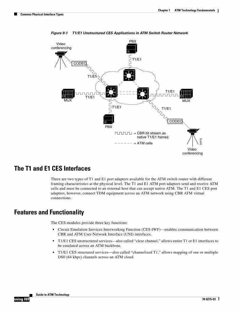
R
Chapter 1 ATM Technology FundamentalsCommon Physical Interface Types
Figure 9-1 T1/E1 Unstructured CES Applications in ATM Switch Router Network
The T1 and E1 CES InterfacesThere are two types of T1 and E1 port adapters available for the ATM switch router with different framing characteristics at the physical level. The T1 and E1 ATM port adapters send and receive ATM cells and must be connected to an external host that can accept native ATM. The T1 and E1 CES port adapters, however, connect TDM equipment across an ATM network using CBR ATM virtual connections.
Features and FunctionalityThe CES modules provide three key functions:
• Circuit Emulation Services Interworking Function (CES-IWF)—enables communication between CBR and ATM User-Network Interface (UNI) interfaces.
• T1/E1 CES unstructured services—also called “clear channel,” allows entire T1 or E1 interfaces to be emulated across an ATM backbone.
• T1/E1 CES structured services—also called “channelized T1,” allows mapping of one or multiple DS0 (64 kbps) channels across an ATM cloud.
PBX
PBX
Video conferencing
Video conferencing
T1/E1
T1/E1
T1/E1 T1/E1
T1/E1
T1/E1MUXMUX
2441
5
CODEC
= CBR bit stream as native T1/E1 frames
CODEC
= ATM cells
unning H/F 4#Guide to ATM Technology
78-6275-03

Chapter 1 ATM Technology FundamentalsCommon Physical Interface Types
Figure 9-2 shows an example of using the CES modules in an ATM network for both unstructured and structured services.
Figure 9-2 Circuit Emulation Services Supported by CES Modules
CES-IWF
CES-IWF is based on an ATM Forum standard that allows communication between CBR and ATM UNI interfaces, that is, between non-ATM telephony devices (such as classic PBXs or TDMs) and ATM devices (such as an ATM switch or router with an ATM interface). CES-IWF works by packaging incoming native T1 or E1 frames into AAL1 cells at the ingress, and performing the opposite function at the egress.
The CES-IWF provided by the ATM switch router allows migration from interconnecting T1/E1 CBR data communications services over separate leased lines to interconnecting those services over the same ATM cloud that carries data traffic.
Figure 9-3 illustrates the use of CES-IWF between non-ATM devices (traditional PBXs) and other end devices. In the case of communication between two non-ATM end devices (traditional PBXs), CBR data in native T1 format received from an edge device on one side of the network is segmented into ATM cells and propagated through the ATM network. After traversing the network, the ATM cells are reassembled into a CBR bit stream that matches the original user data. This native T1 CBR data is then passed out of the network to the edge device at the destination endpoint. In the case of communication between the traditional PBX and the ATM data service unit (DSU), it is the DSU that performs the reassembly into the CBR bit stream for its attached PBX. Both cases illustrate the use of CES-IWF.
PBXPBX
PBX
MUX MUX
128 kbps (2 x 64)
128 kbps (2 x 64)320 kbps (5 x 64) 320 kbps (5 x 64)
T1/E1 T1/E1
T1/E1 structured servicesT1/E1 unstructured services
2441
3
T1/E1
T1/E1
T1/E1
1-15Guide to ATM Technology
78-6275-03
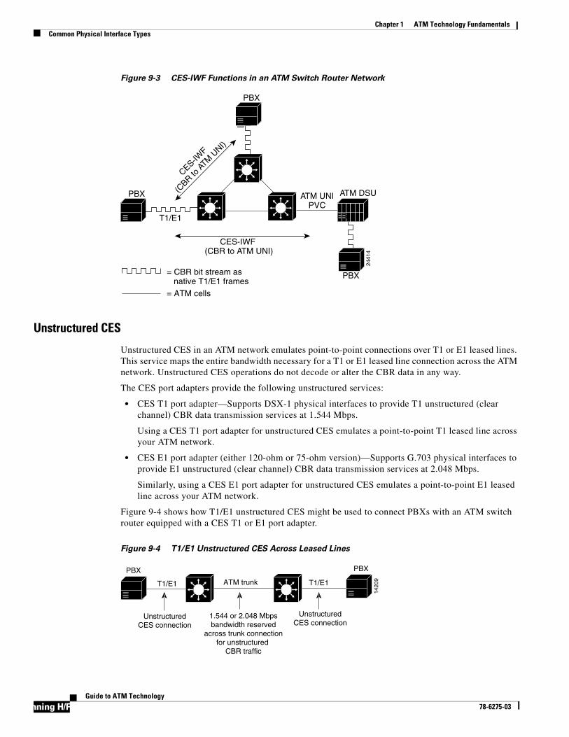
R
Chapter 1 ATM Technology FundamentalsCommon Physical Interface Types
Figure 9-3 CES-IWF Functions in an ATM Switch Router Network
Unstructured CES
Unstructured CES in an ATM network emulates point-to-point connections over T1 or E1 leased lines. This service maps the entire bandwidth necessary for a T1 or E1 leased line connection across the ATM network. Unstructured CES operations do not decode or alter the CBR data in any way.
The CES port adapters provide the following unstructured services:
• CES T1 port adapter—Supports DSX-1 physical interfaces to provide T1 unstructured (clear channel) CBR data transmission services at 1.544 Mbps.
Using a CES T1 port adapter for unstructured CES emulates a point-to-point T1 leased line across your ATM network.
• CES E1 port adapter (either 120-ohm or 75-ohm version)—Supports G.703 physical interfaces to provide E1 unstructured (clear channel) CBR data transmission services at 2.048 Mbps.
Similarly, using a CES E1 port adapter for unstructured CES emulates a point-to-point E1 leased line across your ATM network.
Figure 9-4 shows how T1/E1 unstructured CES might be used to connect PBXs with an ATM switch router equipped with a CES T1 or E1 port adapter.
Figure 9-4 T1/E1 Unstructured CES Across Leased Lines
PBX
PBX
PBX
T1/E1
ATM UNIPVC
ATM DSU
2441
4
CES-IWF (CBR to ATM UNI)
CES-IWF
(CBR to
ATM
UNI)
= CBR bit stream as native T1/E1 frames= ATM cells
PBX PBX
T1/E1 T1/E1ATM trunk
UnstructuredCES connection
UnstructuredCES connection
1.544 or 2.048 Mbpsbandwidth reserved
across trunk connectionfor unstructured
CBR traffic
1420
9
unning H/F 4#Guide to ATM Technology
78-6275-03

Chapter 1 ATM Technology FundamentalsCommon Physical Interface Types
Structured CES
Structured CES is designed to emulate point-to-point fractional T1 (N x 64 kbps) connections. N x 64 refers to a circuit bandwidth (data transmission speed) provided by the aggregation of N x 64-kbps channels. The 64-kbps data rate, or the DS0 channel, is the basic building block of the T carrier systems (T1, T2, and T3).
With T1/E1 structured CES, networks can be simplified by eliminating TDM devices and allocating T1/E1 bandwidth to PBXs and teleconferencing equipment. In addition, the Simple Gateway Control Protocol (SGCP) can be used to control structured CES circuits for voice over ATM. See the “Simple Gateway Control Protocol” section on page 9-27.
The CES modules provide the following structured services:
• CES T1 port adapter—Supports DSX-1 physical interfaces to provide T1 channelized data transmission services at a rate of 1.544 Mbps.
Using a CES T1 port adapter, you can map one or more digital signal level 0 (DS0) channels to an ATM virtual circuit to be connected across an ATM network. Each T1 port has up to 24 DS0 time slots per T1 port for allocation to structured CES circuits. Each time slot can transmit CBR data at a rate of 64 kbps. This represents a total CBR data transmission capacity of 1.536 Mbps (24 x 64 kbps).
• CES E1 port adapter—Supports G.703 physical interfaces to provide E1 channelized data transmission services at a rate of 2.048 Mbps.
Using either the 120- or 75-ohm version of a CES E1 port adapter, you can map a single DS0 channel (64 kbps) or multiple DS0 channels across an ATM network. Each E1 port has up to 31 DS0 available time slots for allocation to structured CES circuits. Each time slot can transmit CBR data at a rate of 64 kbps. This represents a total CBR data transmission capacity of 1.984 Mbps (31 x 64 kbps).
Note With channel-associated signaling enabled, the effective data transfer rate of the circuit is limited to 56 kbps. The “Channel-Associated Signaling and On-Hook Detection for Structured CES” section on page 9-8 describes the CAS mechanism.
By supporting T1/E1 structured CES, the CES module can function in the same way as a classic digital access and crossconnect system (DACS) switch. Figure 9-5 illustrates the digital crossconnect and channelized mapping functions supported by an ATM switch router equipped with a CES module.
1-15Guide to ATM Technology
78-6275-03

R
Chapter 1 ATM Technology FundamentalsCommon Physical Interface Types
Figure 9-5 DACS Function of CES Modules
Either single or multiple DS0 time slots can be mapped across the ATM network. Each time slot (or DS0 channel) can transmit CBR data at a rate of 64 kbps. Note also that multiple N x 64 circuits can be connected to a single port, using separate time slots.
In Figure 9-6, for example, structured CES allows DS0 timeslots to be combined into circuits and transported using ATM PVCs. The PVCs can be routed to many different destination CES interfaces. Similarly, circuits from many different CES interfaces can be interconnected to a single CES interface, where the various circuit DS0 timeslots are interleaved to form an outgoing T1 bit stream. Thus, you can combine structured CBR data in a highly flexible way for transport across an ATM network.
(1 x 64)
(1 x 64)
(1 x 64)(1 x 64)
(12 x 64)
(12 x 64)
(12 x 64)(12 x 64)
1249
5
T1/E1
T1/E1
T1/E1
T1/E1
T1/E1
ATM switch
ATM switchATM switch
unning H/F 4#Guide to ATM Technology
78-6275-03
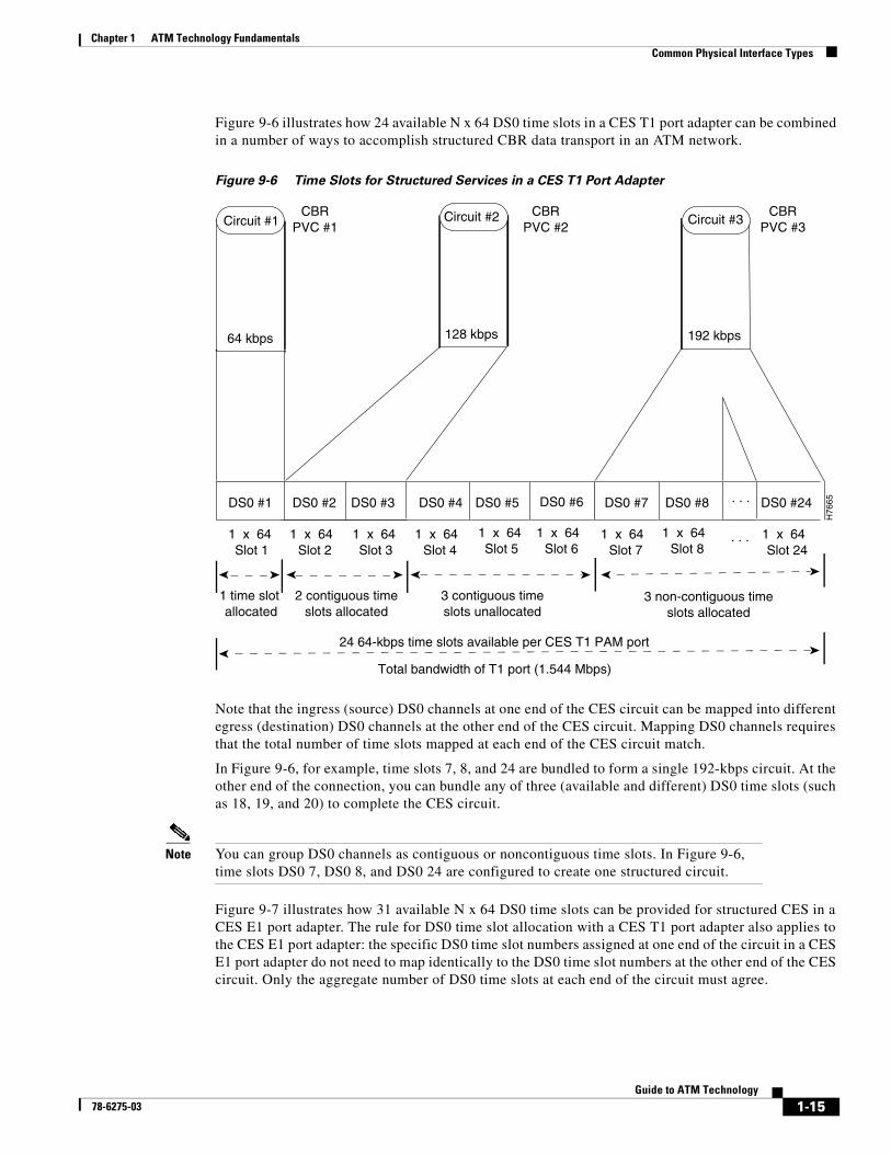
Chapter 1 ATM Technology FundamentalsCommon Physical Interface Types
Figure 9-6 illustrates how 24 available N x 64 DS0 time slots in a CES T1 port adapter can be combined in a number of ways to accomplish structured CBR data transport in an ATM network.
Figure 9-6 Time Slots for Structured Services in a CES T1 Port Adapter
Note that the ingress (source) DS0 channels at one end of the CES circuit can be mapped into different egress (destination) DS0 channels at the other end of the CES circuit. Mapping DS0 channels requires that the total number of time slots mapped at each end of the CES circuit match.
In Figure 9-6, for example, time slots 7, 8, and 24 are bundled to form a single 192-kbps circuit. At the other end of the connection, you can bundle any of three (available and different) DS0 time slots (such as 18, 19, and 20) to complete the CES circuit.
Note You can group DS0 channels as contiguous or noncontiguous time slots. In Figure 9-6, time slots DS0 7, DS0 8, and DS0 24 are configured to create one structured circuit.
Figure 9-7 illustrates how 31 available N x 64 DS0 time slots can be provided for structured CES in a CES E1 port adapter. The rule for DS0 time slot allocation with a CES T1 port adapter also applies to the CES E1 port adapter: the specific DS0 time slot numbers assigned at one end of the circuit in a CES E1 port adapter do not need to map identically to the DS0 time slot numbers at the other end of the CES circuit. Only the aggregate number of DS0 time slots at each end of the circuit must agree.
DS0 #4 DS0 #5 DS0 #6 DS0 #7 DS0 #8 DS0 #24. . .
. . .
DS0 #1 DS0 #2 DS0 #3
Circuit #1 Circuit #2 Circuit #3CBR
PVC #3CBR
PVC #2CBR
PVC #1
Total bandwidth of T1 port (1.544 Mbps)
H76
65
1 x 64 Slot 1
1 x 64 Slot 2
1 x 64 Slot 3
1 x 64 Slot 4
1 x 64 Slot 5
1 x 64 Slot 6
1 x 64 Slot 7
1 x 64 Slot 8
1 x 64 Slot 24
64 kbps 128 kbps 192 kbps
1 time slot allocated
2 contiguous timeslots allocated
3 contiguous timeslots unallocated
3 non-contiguous timeslots allocated
24 64-kbps time slots available per CES T1 PAM port
1-15Guide to ATM Technology
78-6275-03
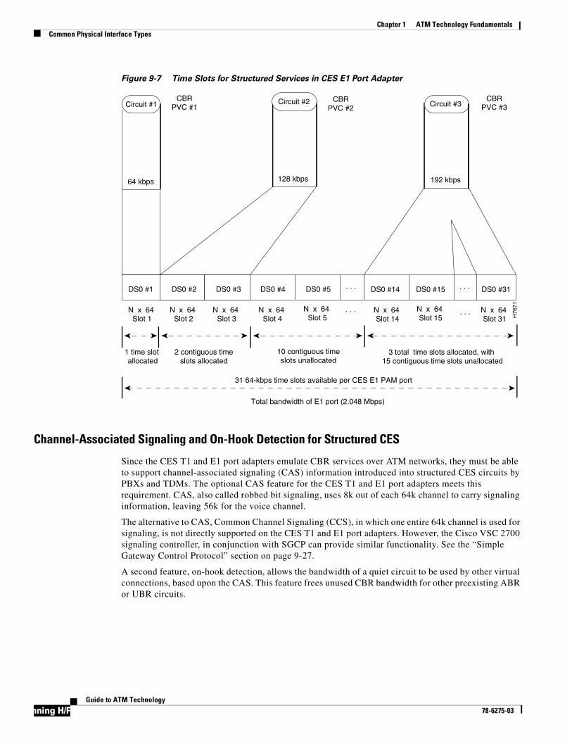
R
Chapter 1 ATM Technology FundamentalsCommon Physical Interface Types
Figure 9-7 Time Slots for Structured Services in CES E1 Port Adapter
Channel-Associated Signaling and On-Hook Detection for Structured CES
Since the CES T1 and E1 port adapters emulate CBR services over ATM networks, they must be able to support channel-associated signaling (CAS) information introduced into structured CES circuits by PBXs and TDMs. The optional CAS feature for the CES T1 and E1 port adapters meets this requirement. CAS, also called robbed bit signaling, uses 8k out of each 64k channel to carry signaling information, leaving 56k for the voice channel.
The alternative to CAS, Common Channel Signaling (CCS), in which one entire 64k channel is used for signaling, is not directly supported on the CES T1 and E1 port adapters. However, the Cisco VSC 2700 signaling controller, in conjunction with SGCP can provide similar functionality. See the “Simple Gateway Control Protocol” section on page 9-27.
A second feature, on-hook detection, allows the bandwidth of a quiet circuit to be used by other virtual connections, based upon the CAS. This feature frees unused CBR bandwidth for other preexisting ABR or UBR circuits.
DS0 #4 DS0 #5 DS0 #14 DS0 #15 DS0 #31. . . . . .
. . .. . .
DS0 #1 DS0 #2 DS0 #3
Circuit #1 Circuit #2 Circuit #3CBR
PVC #3CBR
PVC #2CBR
PVC #1
Total bandwidth of E1 port (2.048 Mbps)
H76
71
N x 64 Slot 1
N x 64 Slot 2
N x 64 Slot 3
N x 64 Slot 4
N x 64 Slot 5
N x 64 Slot 14
N x 64 Slot 15
N x 64 Slot 31
64 kbps 128 kbps 192 kbps
1 time slot allocated
2 contiguous timeslots allocated
10 contiguous timeslots unallocated
3 total time slots allocated, with 15 contiguous time slots unallocated
31 64-kbps time slots available per CES E1 PAM port
unning H/F 4#Guide to ATM Technology
78-6275-03
Chapter 1 ATM Technology FundamentalsCommon Physical Interface Types
These features can be configured for structured CES in the following ways:
• CAS not enabled (the default state)
In this case, the CES module does not sense the CAS information (carried as ABCD bits in the CBR bit stream) and does not provide support for CAS functions.
• CAS enabled without on-hook detection
In addition to packaging incoming CBR data into ATM adaptation layer 1 (AAL1) cells in the usual manner for transport through the network, the CES module in the ingress ATM switch router (see Figure 9-8) senses the ABCD bit patterns in the incoming data, incorporates these patterns in the ATM cell stream, and propagates the cells to the next node in the network. The ATM cells flow across the network from link to link until reaching the egress ATM switch router node.
At the egress node, the CES module strips off the ABCD bit patterns carried by the ATM cells, reassembles the CAS ABCD bits and the user’s CBR data into their original form, and passes the frames out of the ATM network on the proper DS0 time slot.
Note All these processes occur transparently.
• CAS and on-hook detection enabled
The CAS and on-hook detection features work together to allow an ingress node in an ATM network to monitor on-hook and off-hook conditions for a specified 1 x 64 structured CES circuit. As implied by 1 x 64, the on-hook detection (or bandwidth-release) feature is supported only in a structured CES circuit with a single DS0 time slot at each end of the connection, as shown in Figure 9-8.
For structured CES, you can invoke CAS with the ability to detect on-hook or off-hook conditions for any given structured CES circuit. The hook state indicates the following:
– On-hook—Circuit is idle or unconnected.
– Off-hook—Circuit is in use and connected.
The CAS mechanism allows dynamically allocated T1/E1 bandwidth and is released by hard PVCs or soft PVCs configured for structured CES.
When you configure CAS, the ingress CES module monitors the ABCD bits in the incoming CBR bit stream to detect on-hook and off-hook conditions in the circuit. In an off-hook condition, all the bandwidth provided for the specified CES circuit is used to transport ATM AAL1 cells across the network from the ingress node to the egress node.
Conversely, in an on-hook condition, the network periodically sends dummy ATM cells from the ingress node to the egress node to maintain the connection. However, these dummy cells consume only a fraction of the circuit’s reserved bandwidth, leaving the rest of the bandwidth available for other network traffic. This bandwidth-release feature enables the network to make more efficient use of its resources by making unused bandwidth available to bursting or oversubscribed traffic. However, the released bandwidth cannot be reserved by other virtual connections.
Note The on-hook detection feature requires customer premises equipment (CPE) that supports on-hook.
1-15Guide to ATM Technology
78-6275-03

R
Chapter 1 ATM Technology FundamentalsCommon Physical Interface Types
Figure 9-8 CAS in a Structured CES Circuit
Enabling the CAS feature for a CES circuit limits the bandwidth of the DS0 channel to 56 kbps for user data, since CAS functions consume 8 kbps of channel bandwidth for transporting the ABCD signaling bits. These signaling bits are passed transparently from the ingress node to the egress node as part of the ATM AAL1 cell stream.
In summary, when you enable the optional CAS and on-hook detection features, the following conditions apply:
• The permanent virtual channel connection (PVCC) provided for the CES circuit always exists.
• The bandwidth for the CES circuit is always reserved.
• During an on-hook state, most of the bandwidth reserved for the CES circuit is not in use. (Dummy cells are occasionally sent from the ingress node to the egress node to maintain the connection.) This unused bandwidth is therefore available when other network traffic, such as ABR traffic, bursts or is oversubscribed.
• During an off-hook state, all the bandwidth reserved for the CES circuit is dedicated to that circuit.
Advantages
Potential advantages of using CES in your ATM network include the following:
• Native T1 handoff allows you to connect directly to a PBX or other TDM device without that device knowing anything about ATM.
• Interconnecting PBXs and TDM devices over an ATM network allows you to take advantage of increased bandwidth, save on leased line costs, and reduce the amount of equipment, such as DSUs and MUXs, required for separate infrastructures.
Limitations
Potential limitations of CES include the following:
• Like traditional TDM, CBR virtual connections used by CES do not offer the statistical multiplexing benefits of other ATM services.
• Clocking, if not properly configured, can cause problems, particularly when there are multiple clocking sources.
PBXPBX
T1/E1T1/E1
= CBR bit stream
= ATM cells
Egress node BDS0 time slot 4
Ingress node ADS0 time slot 2
1421
1
unning H/F 4#Guide to ATM Technology
78-6275-03

Chapter 1 ATM Technology FundamentalsCommon Physical Interface Types
Network Clocking for CES and CBR TrafficFor your CES environment to function properly, clocking must be carefully set up. Clock sources and their priorities, along with a distribution mode, must be properly configured, as described in Chapter 8, “Network Clock Synchronization.”
The CES port adapters are capable of using three clocking modes to meet the timing requirements of CBR data:
• Synchronous—the default clocking mode for CES. If you have a single PRS, such as a clock signal from a telephone company, you should use synchronous mode. If you are using structured CES, you must use synchronous mode.
• Synchronous residual time stamp (SRTS)—allows equipment at the edges of a network to use a clocking signal that is different (and completely independent) from the clocking signal being used in the ATM network. SRTS mode also allows two CPEs to have different clocks.
• Adaptive—typically used when it is not possible to implement either synchronous or SRTS mode. This is the least precise and least recommended method.
Table 9-1 summarizes, in order of preference, the characteristics of the three clocking modes you can configure on a CES module.
Although the wander and jitter characteristics of these clocking modes differ, all clocking modes preserve the integrity of the your CBR data, ensuring error-free data transport from source to destination. The differences among the three modes are further described in the following sections.
Table 9-1 Characteristics of CES Clocking Modes
Clocking Mode Advantages Limitations
Synchronous Supports both unstructured (clear channel) and structured CBR traffic.
Exhibits superior control of wander and jitter.
Requires a PRS and network clock synchronization services.
Ties the CES interface to the network clock synchronization services clocking signal (PRS).
SRTS Conveys externally generated user clocking signal through an ATM network, providing an independent clocking signal for each CES circuit.
Requires a PRS and network clock synchronization services.
Supports only unstructured (clear channel) CBR traffic.
Exhibits moderate control of wander and jitter.
Adaptive Does not require a PRS or network clock synchronization services.
Supports only unstructured (clear channel) CBR traffic.
Exhibits poorest control of wander and jitter.
1-15Guide to ATM Technology
78-6275-03

R
Chapter 1 ATM Technology FundamentalsCommon Physical Interface Types
Synchronous Clocking Synchronous clocking mode is the only one that supports full CES functionality. SRTS and adaptive clocking do not support structured CES. In addition, synchronous clocking is typically used in public telephony systems, making a precision reference signal readily and widely available for synchronizing CBR data transport. With synchronous clocking mode, every device must get its clocking from a single PRS, such as a PBX connecting to a public telephone network.
Figure 9-9, for example, shows how a PRS for synchronous clocking can be provided to an edge node of an ATM network and propagated through the network to synchronize the flow of CBR data between the communicating ATM end nodes.
In this network scenario, a PRS is available to the network by the PBX at the edge of the network. The PRS is present at the port of a CES module in edge node A (the ingress node). From there, the PRS is propagated into the first ATM network through an ATM port and conveyed across an OC-3 trunk to an adjacent ATM network. This same clocking signal is then used to synchronize the handling of CBR data in edge node B (the egress node).
Figure 9-9 Synchronous Clocking in an ATM Switch Router Network
Configuration Overview
Since synchronous clocking is the default for CES, you do not need to perform any per-interface configuration when using this mode. This assumes that you have one PRS and have properly configured your network clocking, as described in Chapter 8, “Network Clock Synchronization.”
SRTS Clocking Synchronous residual time stamp (SRTS) clocking mode is typically used when there are multiple different clock sources; for example, a when you already have your ATM network synchronized to a reference source, then add a PBX that receives its clock from another service provider source. If you want to avoid resynchronizing your network to their source, SRTS provides a solution by reconciling the different timing signals in the course of CBR data transport through the ATM network.
OC-3/OC-12trunk
PBX
CBR port
ATM portATM port
Edge nodeB
Edge nodeA
1420
1
PRS
T1/E1T1/E1
unning H/F 4#Guide to ATM Technology
78-6275-03

Chapter 1 ATM Technology FundamentalsCommon Physical Interface Types
A common scenario for using SRTS clocking is when your edge equipment is driven by a different clocking signal than that being used in the ATM network. For example, user equipment at the edges of the network can be driven by clock A, while the devices within the ATM network are being driven by clock B. Figure 9-10 shows such an operating scenario, in which a timing signal is provided to edge nodes independently from the ATM network.
Figure 9-10 SRTS Clocking in an ATM Switch Router Network
Using Figure 9-10, assume that the user of edge node 1 wants to send CBR data to a user at edge node 3. In this scenario, SRTS clocking works as follows:
1. Clock A is driving the devices within the ATM network.
2. At edge node 1, the user introduces CBR traffic into the ATM network according to clock B.
3. As edge node 1 segments the CBR bit stream into ATM cells, it measures the difference between user clock B, which drives it, and network clock A.
4. As edge node 1 generates the ATM cell stream, it incorporates this delta value into every eighth cell.
5. The cells then propagate through the network in the usual manner.
6. As destination edge node 3 receives the cells, this node not only reassembles the ATM cells into the original CBR bit stream, but also reconciles, or reconstructs, the user clock B timing signal from the delta value carried within every eighth ATM cell.
Thus, during SRTS clocking, CBR traffic is synchronized between the ingress (segmentation) side of the CES circuit and the egress (reassembly) side of the circuit according to user clock signal B, while the ATM network continues to function according to clock A.
PBX 2
PBX 3
1420
2
PBX 1
Clock A
Clock A
Clock A Clock A
Clock A - Timing reference signal for ATM network Clock B - Timing reference signal for CBR device.
Timingnetwork
forclock B
Edge node 1
Edge node 2
Edge node 3
ATMnetwork
T1/E1
T1/E1
T1/E1
Clock B
Clock B Clock B
1-15Guide to ATM Technology
78-6275-03
R
Chapter 1 ATM Technology FundamentalsCommon Physical Interface Types
Configuration Overview
Configuring SRTS clocking for CES requires the following steps:
Step 1 Configure the global clocking as described in Chapter 8, “Network Clock Synchronization.”
Step 2 From interface configuration mode, enable SRTS clocking mode on the CES interfaces.
Adaptive Clocking The name adaptive clocking mode reflects the fact that the rate at which CBR data is propagated through an ATM network is driven essentially by the rate at which CBR data is introduced into the network by the user’s edge equipment. The actual rate of CBR data flow through the network might vary from time to time during adaptive clocking, depending on how rapidly (or how slowly) CBR data is being introduced into the network. Nevertheless, CBR data transport through the network occurs in a “pseudo synchronous” manner that ensures the integrity of the data.
Adaptive clocking requires neither the network clock synchronization service nor a global PRS for effective handling of CBR traffic. Rather than using a clocking signal to convey CBR traffic through an ATM network, adaptive clocking in a CES module infers appropriate timing for data transport by calculating an “average” data rate upon arrival and conveying that data to the output port of the module at an equivalent rate.
For example, if CBR data is arriving at a CES module at a rate of so many bits per second, then that rate is used, in effect, to govern the flow of CBR data through the network. What happens behind the scenes, however, is that the CES module automatically calculates the average data rate using microcode (firmware) built into the board. This calculation occurs dynamically as user data traverses the network.
When the CES module senses that its segmentation and reassembly (SAR) buffer is filling up, it increases the rate of the transmit (TX) clock for its output port, thereby draining the buffer at a rate that is consistent with the rate of data arrival.
Similarly, the CES module slows down the transmit clock of its output port if it senses that the buffer is being drained faster than CBR data is being received. Adaptive clocking attempts to minimize wide excursions in SAR buffer loading, while at the same time providing an effective means of propagating CBR traffic through the network.
Relative to the other clocking modes, implementing adaptive clocking is simple and straightforward. It does not require network clock synchronization services, a PRS, or the advance planning typically associated with developing a logical network timing map. However, adaptive clocking does not support structured CES, and it exhibits relatively high wander characteristics.
Configuration Overview
Unlike synchronous or SRTS modes, configuring adaptive clocking mode for CES does not require selection of clocking sources, priorities, and distribution mode. You must only enable adaptive clocking from interface configuration mode on each of the CES interfaces.
CES ConfigurationsThis section provides some general guidelines and considerations when configuring CES connections. This section also includes examples of various types of unstructured and structured service connections you can configure for CES.
unning H/F 4#Guide to ATM Technology
78-6275-03
Chapter 1 ATM Technology FundamentalsCommon Physical Interface Types
Before You BeginBefore you begin configuring physical interfaces and virtual circuits for CES operation, you should be aware of the information you need and the associated tasks:
• Network clocking
You must have clocking properly configured for CES operations to be successful. Configuring synchronous clocking is described in Chapter 8, “Network Clock Synchronization.” Special clocking cases for CES are described in the “Network Clocking for CES and CBR Traffic” section on page 9-11 in this chapter.
• Service type
You must decide whether to use unstructured or structured services. See the “Unstructured CES” section on page 9-4 and the “Structured CES” section on page 9-5 for descriptions.
• Physical level characteristics:
– Framing type
– Line buildout
– Line code type
– Loopback test method
Refer to your ATM switch router software documentation for details on configuring these and other physical level parameters.
• Cell Delay Variation (CDV)
CDV can be critical due to the delay-sensitive nature of CBR data; refer to the “About Cell Delay Variation” section on page 9-15.
• PVC (hard, soft)
You must decide whether to use hard or soft PVCs. Manual configuration is required for hard PVCs, while soft PVCs are set up through signaling. Also, soft PVCs can reroute in the event of failure, while hard PVCs cannot. For more information, see the “General Procedure for Creating Soft PVCCs for CES” section on page 9-16.
About Cell Delay VariationCell delay variation (CDV) refers to the distortion caused by change in interarrival times between cells, also known as jitter, measured in microseconds.
Each end-to-end CES circuit exhibits delay characteristics, based on the following factors:
• The delay characteristics of the individual devices participating in the CES circuit.
Each network device contributes some increment of delay, reflecting the unique electrical characteristics of that device.
• The number of intermediate hops through which the CBR data must pass in traversing the network from source to destination.
• The type and speed of the trunk lines interconnecting the ATM networks.
• The volume of traffic being handled by the trunk lines at any given time; that is, the degree to which the network is experiencing congestion conditions.
1-15Guide to ATM Technology
78-6275-03
R
Chapter 1 ATM Technology FundamentalsCommon Physical Interface Types
The network designer or administrator calculates a CDV value for each hop in the data path as a means of establishing a maximum allowable CDV value for the network as a whole. To some degree, the network’s maximum allowable CDV value is a measure of the network’s expected performance. By establishing this CDV threshold for the network, appropriate buffer sizing can be derived for the network devices involved in any given CES circuit, ensuring that the network operates as expected.
In a CES module, for example, the maximum allowable CDV value for the network is used to determine an appropriate size (depth) for the SAR buffer built into the board. This sizing of the SAR buffer is done to prevent buffer overflow or underflow conditions. An overflow condition can cause a loss of frames, while an underflow condition can cause frames to be repeated.
The actual CDV value for a circuit varies according to the particular data path used for the circuit. Consequently, the depth of the SAR buffer increases or decreases in proportion to the CDV value for the CES circuit being set up.
Tips You can issue the CLI show ces circuit interface command in an unstructured circuit to measure the current CDV value. In many cases the configured default value is satisfactory.
For an unstructured hard PVC, the CDV value for the circuit (including all hops) must not exceed a maximum allowable CDV value.
For an unstructured soft PVC, the network automatically determines the best data path through the network and handles the routing of CBR traffic. The network accomplishes this task dynamically through the ATM connection admission control (CAC) mechanism. The CAC mechanism determines the best path through the network by executing a routing algorithm that consults local routing tables in network devices.
If the requested data path is equal to or less than the maximum allowable CDV value established by the network administrator, the connection request is granted. If the requested CES circuit exceeds the maximum allowable CDV value, the connection request is denied.
For example, when a user requests a connection from source node A at one edge of the network to destination node B at the opposite edge of the network, the CAC mechanism accounts for the CDV value for each hop in the requested connection to determine a suitable path through the network that does not exceed the network’s maximum allowable CDV value.
General Procedure for Creating Soft PVCCs for CESYou can create either hard PVCCs or soft PVCCs, depending on your particular CES application requirements, for use in your CES operations. This section provides a general procedure for configuring soft PVCCs for CES.
The following steps must be performed in the prescribed order when you configure soft PVCCs for either unstructured or structured CES:
Note The steps in these guidelines assume that you have already configured circuits on the CES interfaces. If you have not, you will not see addresses in some displays, or the output will be null.
Step 1 Determine which CES interfaces are currently configured in your ATM switch router chassis. The show ces status command displays this information for you.
Step 2 Determine which two ports you want to define as participants in the soft PVCC.
unning H/F 4#Guide to ATM Technology
78-6275-03

Chapter 1 ATM Technology FundamentalsCommon Physical Interface Types
Step 3 Decide which of the two ports you want to designate as the destination (or passive) side of the soft PVCC.
Note This is an arbitrary decision—you can choose either port as the destination end of the circuit. However, you must decide which port is to function in this capacity and proceed accordingly.
Step 4 Configure the destination (passive) side of the soft PVCC.
You must configure the destination end of the soft PVCC first, as this end defines an ATM Forum-compliant CES-IWF ATM address for that port.
Step 5 Retrieve the CES-IWF ATM address of the soft PVCC’s destination end. You can use the show ces address command to display the CES-IWF ATM addresses.
You must determine this address, as well as the VPI/VCI values for the circuit (see Step 6), and use these elements as part of the command string when you configure the source (active) end of the soft PVCC (see Step 8).
Step 6 Retrieve the VPI/VCI values for the circuit. You can use the show ces circuit command to display the VPI/VCI values.
Step 7 Shut down the interface.
Step 8 Configure the source (active) end of the soft PVCC last, using the information derived from Step 5 and Step 6.
You must configure the source end of the soft PVCC last, because that end not only defines the configuration information for the source port, but also requires you to enter the CES-IWF ATM address and VPI/VCI values for the destination port.
Step 9 Reenable the interface.
Note The soft PVC route optimization feature is not supported for CBR data.
T1/E1 Unstructured CESThis section provides an overview of the procedures for configuring CES modules for unstructured CES.
The circuit you set up on a CBR port for unstructured service is always identified as circuit 0, since you can establish only one unstructured circuit on any given CBR port. An unstructured circuit uses the entire bandwidth of a T1 or E1 port, as follows:
• A hard PVCC on a T1 or E1 port—At least the entire bandwidth of a T1 port (1.544 Mbps) or an E1 port (2.048 Mbps) is allocated to the soft PVCC along its path as long as the soft PVCC is up. A network failure along the path of the soft PVCC relinquishes this bandwidth until the connection can be set up again.
• A soft PVCC on a T1 or E1 port—The entire bandwidth of a T1 port (1.544 Mbps) or an E1 port (2.048 Mbps) is also allocated manually when you set up the circuit, but this bandwidth is only used by the unstructured circuit when it is active.
1-15Guide to ATM Technology
78-6275-03

R
Chapter 1 ATM Technology FundamentalsCommon Physical Interface Types
Hard PVCCs for Unstructured Services
A CES module converts CBR traffic into ATM cells for propagation through an ATM network. CBR traffic arriving on a given CES module port must first be segmented into ATM cells. This cell stream is then directed to an outgoing ATM port or CBR port using a PVCC.
Note As a general rule when configuring a hard PVCC, you must cross-connect a CBR port and an ATM port in the same ATM switch router chassis.
Figure 9-11 shows an example of using a hard PVCC to connect ATM and CES interface modules for unstructured CES on the ATM switch router.
Figure 9-11 Hard PVCC Configured for Unstructured CES
Configuration Overview
Configuring a hard PVCC, such as the one shown in Figure 9-11, requires the following steps:
Step 1 Display the current CES and ATM interface information. Use this information to identify the source CBR and destination ATM interfaces.
Step 2 From global configuration mode, select the CBR interface to configure and enter interface configuration mode.
Step 3 Configure the CES AAL1 clock mode.
For descriptions of the clocking modes, see the “Network Clocking for CES and CBR Traffic” section on page 9-11.
If you are using synchronous or SRTS clocking mode, you must first configure the global clocking distribution mode for the chassis and the clock source on the interface; you do not need to perform these steps if you are using adaptive clocking. For more information on configuring clock sources, see Chapter 8, “Network Clock Synchronization.”
Step 4 Configure the CES AAL1 service as unstructured (the default).
Step 5 If needed, configure the line coding, framing, and line buildout.
ATM port adapter(module slot 0)
CES port adapter(module slot 1)
Target switch
1249
3
Destination portPort ID - ATM0/0/0
(Explicit VPI 0, VCI 100)
Source port Port ID - CBR0/1/0
(Implicit VPI 0, VCI 16)
Chassis slot 0
CBR-PVC-A
PVC 0
00 1 2 3
Switching
Fabric
unning H/F 4#Guide to ATM Technology
78-6275-03

Chapter 1 ATM Technology FundamentalsCommon Physical Interface Types
Step 6 Configure the CES interface circuit identifier and specify a circuit name.
Step 7 Configure the hard PVCC cross-connect to the ATM interface with VPI/VCI values.
Soft PVCCs for Unstructured Services
In a soft PVCC, as well as a hard PVCC, you configure both ends of the CES circuit. However, a soft PVCC typically involves CES modules at opposite edges of an ATM network, so a soft PVCC can be set up between any two CES modules anywhere in your network.
For guidelines when configuring soft PVCCs, see the “General Procedure for Creating Soft PVCCs for CES” section on page 9-16.
The destination address of a soft PVCC can point to either of the following:
• A port in the same ATM switch router chassis
• A port in any other CES module in the network
Note For simplicity, the procedure in this section assumes that you are creating a soft PVCC between interfaces in the same ATM switch router chassis. In a typical scenario, you would configure a soft PVCC to connect CES interfaces on ATM switch routers at opposite ends of a network, where the CES interfaces are attached to PBXs or other TDM devices.
Figure 9-12 shows a logical representation of the soft PVCC used in the following example procedure.
Figure 9-12 Soft PVCC Configured for Unstructured CES
Configuration Overview
Configuring a soft PVCC for unstructured CES is a two-phase process:
• Phase 1—Configure the destination (passive) side of the soft PVCC.
• Phase 2—Configure the source (active) side of the soft PVCC.
ATM port adapter(module slot 0)
CES port adapter(module slot 1)
Target switch
1249
4
CBR-PVC-A (CBR0/1/0)
(VPI 0, VCI 16)Source (active) side of PVC
CBR-PVC-B(CBR0/1/1)(VPI 0, VCI 1040)Destination (passive) side of PVC
Chassisslot 0
Circuit 0
0 1 2 3
Switching
Fabric
1-15Guide to ATM Technology
78-6275-03

R
Chapter 1 ATM Technology FundamentalsCommon Physical Interface Types
Configuring the destination side of the soft PVCC, as shown in Figure 9-12, requires the following steps:
Step 1 Display the current CES interface information. Use this information to identify the destination CBR interface.
Step 2 From global configuration mode, select the CBR interface to configure and enter interface configuration mode.
Step 3 Configure the CES AAL1 clock mode.
For descriptions of the clocking modes, see the “Network Clocking for CES and CBR Traffic” section on page 9-11.
If you are using synchronous or SRTS clocking mode, you must first configure the global clocking distribution mode for the chassis and the clock source on the interface; you do not need to perform these steps if you are using adaptive clocking. For more information on configuring clock sources, see Chapter 8, “Network Clock Synchronization.”
Step 4 Configure the CES AAL1 service as unstructured (the default).
Step 5 If needed, configure the line coding, framing, and line buildout.
Step 6 Configure the CES interface circuit identifier and specify a circuit name.
Configuring the source side of the soft PVCC requires the following steps:
Step 1 Display the CES interface information for the destination side. Use this information to identify the ATM address and VPI/VCI values to use when configuring the source side of the soft PVCC.
Step 2 From global configuration mode, select the CBR interface to configure and enter interface configuration mode.
Step 3 Configure the CES AAL1 service as unstructured (the default).
Step 4 If needed, configure the line coding, framing, and line buildout.
Step 5 Configure the CES interface circuit identifier and specify a circuit name.
Step 6 Configure the soft PVCC to the destination CES-IWF ATM address and VPI/VCI of the circuit.
T1/E1 Structured CESThis section provides an overview of the procedures you use when configuring CES modules for structured (N x 64 kbps) CES.
An important distinction between structured and unstructured CES is that structured CES allows you to allocate the entire T1/E1 bandwidth. Structured CES only uses the T1/E1 bandwidth actually required to support the active structured circuit(s) you configure. For example, configuring a CES module for structured services allows you to define multiple hard PVCCs or soft PVCCs for any CES T1 or E1 port.
In both module types, any bits not available for structured CES are used for framing and out-of-band control.
unning H/F 4#Guide to ATM Technology
78-6275-03

Chapter 1 ATM Technology FundamentalsCommon Physical Interface Types
Note Structured CES requires synchronous clocking mode. See the “Network Clocking for CES and CBR Traffic” section on page 9-11.
Hard PVCCs for Structured Services without CAS
This section describes configuring a hard PVCC for structured CES without channel-associated signaling (CAS).
Figure 9-13 illustrates a hard PVCC for a structured CES connection configured with the following parameters:
• Four time slots (DS0 channels 1 to 3, and 7) are configured for a circuit named CBR-PVC-A.
• CAS is not used.
• ATM port 0/0/0 in the ATM switch router chassis is designated as the destination port of the hard PVCC.
Figure 9-13 Hard PVCC Configured for Structured CES
Configuration Overview
Configuring a hard PVCC for structured CES without CAS requires the following tasks:
Step 1 Display the current CES and ATM interface information. Use this information to identify the source CBR and destination ATM interfaces.
Step 2 From global configuration mode, select the CBR interface to configure and enter interface configuration mode.
Step 3 Configure the CES AAL1 service as structured.
When the AAL1 service is configured as structured, clocking mode is synchronous by default. No other clocking configuration for CES is required, assuming that you have properly configured the global clocking distribution mode for the chassis and the clock source on the interface (network-derived by default). For more information on configuring clock sources, see Chapter 8, “Network Clock Synchronization.”
ATM port adapter(module slot 0)
CES port adapter(module slot 1)
Target switch
1249
7
Destination portPort ID - ATM0/0/0
(Explicit VPI 0, VCI 100)
Source port Port ID - CBR0/1/0
CBR-PVC-A(Implicit VPI 0, VCI 16)
(DSO 1-3, and 7)
Chassisslot 0
00 1 2 3
Switching
Fabric
1-15Guide to ATM Technology
78-6275-03
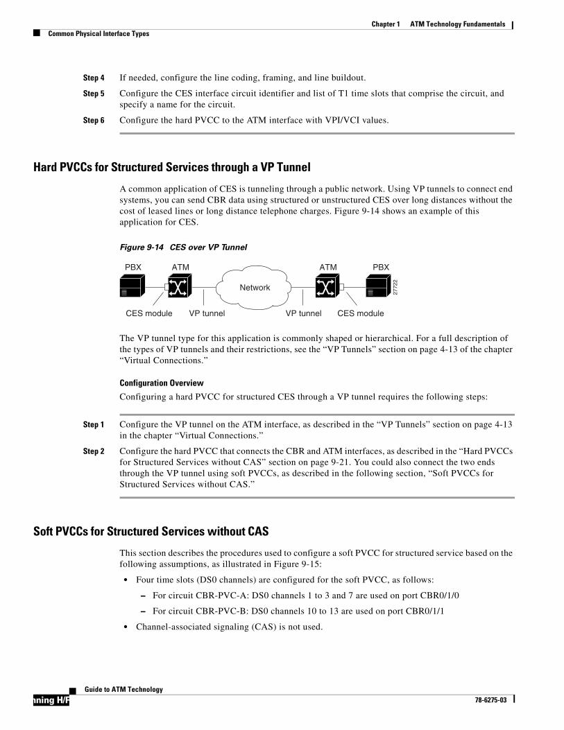
R
Chapter 1 ATM Technology FundamentalsCommon Physical Interface Types
Step 4 If needed, configure the line coding, framing, and line buildout.
Step 5 Configure the CES interface circuit identifier and list of T1 time slots that comprise the circuit, and specify a name for the circuit.
Step 6 Configure the hard PVCC to the ATM interface with VPI/VCI values.
Hard PVCCs for Structured Services through a VP Tunnel
A common application of CES is tunneling through a public network. Using VP tunnels to connect end systems, you can send CBR data using structured or unstructured CES over long distances without the cost of leased lines or long distance telephone charges. Figure 9-14 shows an example of this application for CES.
Figure 9-14 CES over VP Tunnel
The VP tunnel type for this application is commonly shaped or hierarchical. For a full description of the types of VP tunnels and their restrictions, see the “VP Tunnels” section on page 4-13 of the chapter “Virtual Connections.”
Configuration Overview
Configuring a hard PVCC for structured CES through a VP tunnel requires the following steps:
Step 1 Configure the VP tunnel on the ATM interface, as described in the “VP Tunnels” section on page 4-13 in the chapter “Virtual Connections.”
Step 2 Configure the hard PVCC that connects the CBR and ATM interfaces, as described in the “Hard PVCCs for Structured Services without CAS” section on page 9-21. You could also connect the two ends through the VP tunnel using soft PVCCs, as described in the following section, “Soft PVCCs for Structured Services without CAS.”
Soft PVCCs for Structured Services without CAS
This section describes the procedures used to configure a soft PVCC for structured service based on the following assumptions, as illustrated in Figure 9-15:
• Four time slots (DS0 channels) are configured for the soft PVCC, as follows:
– For circuit CBR-PVC-A: DS0 channels 1 to 3 and 7 are used on port CBR0/1/0
– For circuit CBR-PVC-B: DS0 channels 10 to 13 are used on port CBR0/1/1
• Channel-associated signaling (CAS) is not used.
PBX PBXATM ATM
VP tunnelCES module CES moduleVP tunnel
Network
2772
2
unning H/F 4#Guide to ATM Technology
78-6275-03
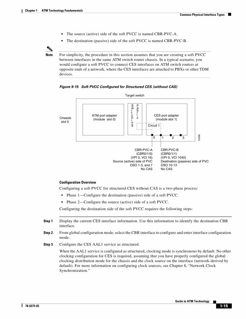
Chapter 1 ATM Technology FundamentalsCommon Physical Interface Types
• The source (active) side of the soft PVCC is named CBR-PVC-A.
• The destination (passive) side of the soft PVCC is named CBR-PVC-B.
Note For simplicity, the procedure in this section assumes that you are creating a soft PVCC between interfaces in the same ATM switch router chassis. In a typical scenario, you would configure a soft PVCC to connect CES interfaces on ATM switch routers at opposite ends of a network, where the CES interfaces are attached to PBXs or other TDM devices.
Figure 9-15 Soft PVCC Configured for Structured CES (without CAS)
Configuration Overview
Configuring a soft PVCC for structured CES without CAS is a two-phase process:
• Phase 1—Configure the destination (passive) side of a soft PVCC.
• Phase 2—Configure the source (active) side of a soft PVCC.
Configuring the destination side of the soft PVCC requires the following steps:
Step 1 Display the current CES interface information. Use this information to identify the destination CBR interface.
Step 2 From global configuration mode, select the CBR interface to configure and enter interface configuration mode.
Step 3 Configure the CES AAL1 service as structured.
When the AAL1 service is configured as structured, clocking mode is synchronous by default. No other clocking configuration for CES is required, assuming that you have properly configured the global clocking distribution mode for the chassis and the clock source on the interface (network-derived by default). For more information on configuring clock sources, see Chapter 8, “Network Clock Synchronization.”
ATM port adapter(module slot 0)
CES port adapter(module slot 1)
Target switch
1249
8
CBR-PVC-A (CBR0/1/0)
(VPI 0, VCI 16)Source (active) side of PVC
DSO 1-3, and 7No CAS
CBR-PVC-B(CBR0/1/1)(VPI 0, VCI 1040)Destination (passive) side of PVCDSO 10-13No CAS
Chassisslot 0
Circuit 1
0 1 2 3
Switching
Fabric
1-15Guide to ATM Technology
78-6275-03

R
Chapter 1 ATM Technology FundamentalsCommon Physical Interface Types
Step 4 If needed, configure the line coding, framing, and line buildout.
Step 5 Configure the CES interface circuit identifier and list of T1 time slots that comprise the circuit, and specify a name for the circuit.
Configuring the source side of a soft PVCC requires the following steps:
Step 1 Display the CES interface information for the destination side. Use this information to identify the ATM address and VPI/VCI values to use when configuring the source side of the soft PVCC.
Step 2 From global configuration mode, select the CBR interface to configure and enter interface configuration mode.
Step 3 Configure the CES AAL1 service as structured.
Step 4 If needed, configure the line coding, framing, and line buildout.
Step 5 Configure the CES interface circuit identifier and list of T1 time slots that comprise the circuit, and specify a name for the circuit.
Step 6 Configure the soft PVCC to the destination CES-IWF ATM address with VPI/VCI values.
Soft PVCCs for Structured Services with CAS
The procedures in this section build on the configuration information in the “Soft PVCCs for Structured Services without CAS” section on page 9-22. However, this procedure enables channel associated signaling (CAS) for the soft PVCC.
The following procedure is based on the following assumptions, as illustrated in Figure 9-16:
• One time slot is configured for the soft PVCC:
– For circuit CBR-PVC-A: DS0 channel 1 on port CBR0/1/0
– For circuit CBR-PVC-B: DS0 channel 10 on port CBR0/1/1
• CAS is enabled for the circuit.
• The signaling mode for the CBR ports is set to robbedbit.
Note For simplicity, the procedure in this section assumes that you are creating a soft PVCC between interfaces in the same ATM switch router chassis. In a typical scenario, you would configure a soft PVCC to connect CES interfaces on ATM switch routers at opposite ends of a network, where the CES interfaces are attached to PBXs or other TDM devices.
unning H/F 4#Guide to ATM Technology
78-6275-03

Chapter 1 ATM Technology FundamentalsCommon Physical Interface Types
Figure 9-16 Soft PVCC Configured for Structured CES with CAS
Configuration Overview
Configuring the destination side of the soft PVCC requires the following steps:
Step 1 Display the current CES interface information. Use this information to identify the destination CBR interface.
Step 2 From global configuration mode, select the CBR interface to configure and enter interface configuration mode.
Step 3 Configure the CES AAL1 service as structured.
When the AAL1 service is configured as structured, clocking mode is synchronous by default. No other clocking configuration for CES is required, assuming that you have properly configured the global clocking distribution mode for the chassis and the clock source on the interface (network-derived by default). For more information on configuring clock sources, see Chapter 8, “Network Clock Synchronization.”
Step 4 If needed, configure the line coding, framing, and line buildout.
Step 5 Configure the DSX1 signal mode to robbedbit.
Step 6 Configure the CES interface circuit identifier and list of T1 time slots that comprise the circuit, and specify a name for the circuit. Specify CAS when configuring the circuit.
Configuring the source soft PVCC requires the following steps:
Step 1 Display the CES interface information for the destination side. Use this information to identify the ATM address and VPI/VCI values to use when configuring the source side of the soft PVCC.
Step 2 From global configuration mode, select the CBR interface to configure and enter interface configuration mode.
Step 3 Configure the CES AAL1 service as structured.
Step 4 If needed, configure the line coding, framing, and line buildout.
ATM port adapter(module slot 0)
CES port adapter(module slot 1)
Target switch
1250
0
CBR-PVC-A (CBR0/1/0)
(VPI 0, VCI 16)Source (active) side of PVC
DSO 1With CAS
CBR-PVC-B(CBR0/1/1)(VPI 0, VCI 1040)Destination (passive) side of PVCDSO 10With CAS
Chassisslot 0
Circuit 1
0 1 2 3
Switching
Fabric
1-15Guide to ATM Technology
78-6275-03

R
Chapter 1 ATM Technology FundamentalsCommon Physical Interface Types
Step 5 Configure the CES interface circuit identifier and list of T1 time slots that comprise the circuit, and specify a name for the circuit. Specify CAS when configuring the circuit.
Step 6 Configure the soft PVCC to the destination CES-IWF ATM address with VPI/VCI values.
Soft PVCCs for Structured Services with CAS and On-Hook Detection Enabled
This section outlines the additional steps that you must take to activate the on-hook detection (bandwidth-release) feature in a 1 x 64 structured soft PVCC CES circuit. For a description of on-hook detection, see the “Channel-Associated Signaling and On-Hook Detection for Structured CES” section on page 9-8.
Configuration Overview
Configuring a soft PVCC for structured services with CAS and on-hook detection requires the following steps:
Step 1 Configure the soft PVCC with CAS enabled, as described in the previous section, “Soft PVCCs for Structured Services with CAS.”
Step 2 Specify on-hook detection in addition to CAS when configuring the circuit.
Multiple Soft PVCCs on the Same CES Port
The procedures in this section describe creating more than one structured service PVCC on the same T1 or E1 port. Figure 9-17 illustrates how you can configure multiple CES circuits on a single T1 or E1 port.
The following assumptions apply to creating multiple soft PVCCs on the same T1 or E1 port, as illustrated in Figure 9-17:
• The source (active) side of a soft PVCC named CBR-PVC-A is already created on port CBR0/1/0.
• The destination (passive) side of a soft PVCC named CBR-PVC-B is already created on port CBR0/1/1.
• A new source (active) side of a soft PVCC named CBR-PVC-AC is created on port CBR0/1/0 of the CES module, thereby creating a multiple CES circuit on this particular port.
• A new destination (passive) side of a soft PVCC named CBR-PVC-CA is created on port CBR0/1/2 of the CES module.
unning H/F 4#Guide to ATM Technology
78-6275-03

Chapter 1 ATM Technology FundamentalsCommon Physical Interface Types
Figure 9-17 Configuring Multiple Soft PVCCs on the Same T1 or E1 Port
Configuration Overview
Configuring the additional soft PVCCs, as shown in Figure 9-17, requires the following steps:
Step 1 On the destination side, configure the parameters for the additional CBR interface and configure the circuit and timeslots. The configuration steps in the “Soft PVCCs for Structured Services without CAS” section on page 9-22 or in the “Soft PVCCs for Structured Services with CAS” section on page 9-24 show how to do this configuration.
Step 2 On the source side, perform the following steps:
a. Configure the additional circuit and time slots on the existing CBR interface.
b. Configure the soft PVCC to cross-connect the two circuits.
Simple Gateway Control ProtocolThe Simple Gateway Control Protocol (SGCP) running on the ATM switch router, in combination with the Cisco VSC 2700, a virtual switch controller, provides switched voice on demand within a campus or metropolitan-area network. Designed to support common channel signaling protocols, this solution can eliminate the need for expensive tandem switches when interconnecting multiple PBXs.
ATM port adapter(module slot 0)
CES port adapter(module slot 1)
Target switch
1249
9
CBR-PVC-A (CBR0/1/0)
Circuit 1(VPI 0, VCI 16)
Source (active) end of PVCDSO 1-3, and 7
No CAS
CBR-PVC-B(CBR0/1/1)Circuit 1(VPI 0, VCI 1040)Destination (passive) end of PVCDSO 10-13No CAS
Chassisslot 0
0 1 2 3
T1/E1
CBR-PVC-AC(CBR0/1/0)
Circuit 224 DS0 time slots
(VPI 0, VCI 32)Source (active) end of PVC
CBR-PVC-CA(CBR0/1/2)Circuit 110 DS0 time slots(VPI 0, VCI 2064)Destination (passive) end of PVC
Switching
Fabric
1-15Guide to ATM Technology
78-6275-03

R
Chapter 1 ATM Technology FundamentalsCommon Physical Interface Types
Networks that include multiple PBXs require a tandem switch, which inter-PBX calls must traverse. To accommodate multiple PBXs, they might all be connected to the tandem switch. Or, as in Figure 9-18, the PBXs might be connected through the ATM network using CES interfaces and clear-channel T1 or E1 links. All inter-PBX calls are required to traverse the tandem switch. This scenario works well where the number of PBXs to be connected is low. As the size of the campus or MAN grow, however, the size of the required tandem PBX also grows, as does the number of primary rate interfaces (PRIs) required.
Figure 9-18 PBXs Connected using Common Channel Signaling and CES
In Figure 9-19 the virtual switch controller (VSC) is connected to an ATM switch router. SGCP, running on both the VSC and the ATM switch router, carries VSC instructions to set up and tear down connections based on the signaling between the VSC and the PBXs. When a call must be established between any two PBXs, the VSC instructs the ATM switch router to provision a soft PVC (64 kbps CBR) between the appropriate two endpoints, providing bandwidth on demand. This reduces the total number of interfaces required and eliminates the need for a tandem PBX.
Figure 9-19 PBXs Connected using the VSC
Building B
PBX
PBX
PBX
PBX
Building C
Building A
Building D
T1/E1
T1/E1
T1/E1
T1/E1T1/E1
T1/E1
OC-3/OC-12 OC-3/OC-12
OC-3/OC-12
OC-3/OC-12 Tandem switch
2443
7
Building B
PBX
PBX
PBX
PBX
Building C
Building A
Building D
T1/E1
T1/E1
T1/E1
T1/E1
T1/E1
VSC 2700
OC-3/OC-12 OC-3/OC-12
OC-3/OC-12
OC-3/OC-12
2443
8
SGCP
Controlpath
SGCP
unning H/F 4#Guide to ATM Technology
78-6275-03

Chapter 1 ATM Technology FundamentalsCommon Physical Interface Types
Additional Advantages
In addition to potentially eliminating the need for the tandem PBX, the VSC and SGCP solution provides the following advantages:
• Reduces the total interfaces required for PBXs.
• Provides bandwidth on demand for devices capable of using common channel signaling over a PRI interface.
• Allows toll bypass where a MAN crosses a local access and transport area (LATA) boundary.
How It WorksSGCP controls Voice over IP gateways by an external call control element (called a call-agent). This feature has been adapted to provide control of ATM switch router CES circuits (called endpoints in SGCP). The resulting system (call-agents and gateways) allows for the call-agent to engage in common channel signaling (CCS) over a 64-kbps CES circuit, governing the interconnection of bearer channels on the CES interface. In this system, the ATM switch router acts as a Voice over ATM gateway.
Figure 9-20 illustrates how 64-kbps CCS channels on the CES T1 and E1 ports are backhauled or carried to the VSC 2700 units.
Figure 9-20 Common Channeling Signaling over a CES Circuit
A single trunk circuit sigA (on ATM switch router A’s CES port) carries or backhauls the CCS control call setup for the port. Trunk circuit sigB also controls a similar port on ATM switch router B. SigA is backhauled over the ATM network to ATM switch router C by a CES soft PVC to a circuit on another CES card port directly attached to a call-agent (VSC 2700 (1)). Similarly, sigB is backhauled to a CES circuit on ATM switch router D.
Both call-agents are configured to handle backhauled signaling circuits to the CES trunk circuits. When a call-setup request is received on sigA by VSC 2700 (1), the VSC 2700 (1) cooperates with VSC 2700 (2) to establish the connection.
VSC 2700 (2) VSC 2700 (1)
CES CES
OC-3OC-3
CES CES
sigB
sigB
sigA
sigA
coop
ATM switch D
ATM switch B ATM switch A
ATM switch C
OC-3 OC-3
port port
port portcallAB
SGCPSGCP
1647
5
1-15Guide to ATM Technology
78-6275-03

R
Chapter 1 ATM Technology FundamentalsCommon Physical Interface Types
To dynamically connect the CES circuits located on ATM switch routers A and B, the call-agents use SGCP to allocate the CES circuits on each switch and then establishes a soft PVC between the switches. The resulting connection is callAB. Call-agents use SGCP to cause the ATM switch routers to set up and delete end-to-end connections between circuits.
Configuration Overview
Configuring SGCP requires the following steps:
Step 1 Enable SGCP on the switch.
SGCP is disabled by default.
Step 2 Configure CES circuits for SGCP.
Enable structured AAL1 service on the CES interface and allocate the time slot to a circuit identifier.
Step 3 Configure SGCP request handling.
Modify the default timeout and retry intervals for SGCP request handling, as needed.
Step 4 Configure call-agent address.
Specify the address of the call agent SGCP is to use.
unning H/F 4#Guide to ATM Technology
78-6275-03

C H A P T E R
Traffic and Resource Managemen
9 C
Traffic and Resource Management
This chapter provides an overview of ATM traffic management in general and describes the related configurable features on the ATM switch router.
Note The information in this chapter is applicable to the Catalyst 8540 MSR, Catalyst 8510 MSR, and LightStream 1010 ATM switch router. For detailed configuration information, refer to the ATM Switch Router Software Configuration Guide and the ATM Switch Router Command Reference publication.
This chapter includes the following sections:
• “Overview” section on page 9-1
• “The Traffic and Service Contract” section on page 9-2
• “Connection Admission Control” section on page 9-5
• “Hardware Resources” section on page 9-12
OverviewTo meet the demands of multiservice networking, in which traffic of varying bandwidth and delay requirements must be simultaneously serviced, sophisticated traffic and resource management mechanisms are needed. To serve these needs, your ATM switch router uses a shared-memory architecture that offers advanced traffic management and congestion control capabilities.
The traffic management features of the ATM switch router provide the following capabilities:
• Integrated support for different types of ATM services
• Flexible policies for bandwidth allocation through controlled link-sharing services
• Effective use of network resources
The congestion control capabilities of the ATM switch router support the following goals:
• Avoid conditions where congestion can occur
• Minimize the effects of congestion when it does occur
• Prevent spreading the congestion state to other parts of the network
Note The specific resource management capabilities of your ATM switch router are platform dependent. Consult the ATM Switch Router Software Configuration Guide for details.
t 9-1

The Traffic and Service Contract
Because ATM networks are designed to carry many different types of traffic, traffic characteristics and QoS requirements of each virtual connection must be described, and delivery of the contract must be guaranteed within the resource allocation policies defined for the network.
These requirements are carried out in three phases:
1 Define the traffic and service contract.
2 Find an acceptable path for the connections.
3 Use hardware resources to honor the terms of the contract for the life of the connection.
The first of these two steps can be considered the connection setup phase, while the third step represents the data flow phase. These three phases and their supporting mechanisms are discussed in the following sections.
The Traffic and Service ContractThe traffic and service contract specifies an envelope that describes the intended data flow and uses the following information:
• A connection traffic descriptor, which includes a service category and applicable parameters
• An optional set of QoS parameters applicable to the service category
Table 9-1 shows which traffic and QoS parameters used on the ATM switch router for the setup of connections in the ATM Forum service categories.
Table 9-1 ATM Service Category Applicable Parameters
When establishing the traffic and service contract, target values for QoS parameters can be used as criteria for the connection setup requirements. These values are either metrics (accumulated over multiple hops of a call) or attributes (a gating criterion that is not accumulated, but is checked at each interface). Maximum cell transfer delay (maxCTD) and peak-to-peak cell delay variation (ppCDV) are metrics, while cell loss ratio is an attribute.
Attributes ATM Layer Service Category
CBR VBR-RT VBR-NRT UBR ABR
PCR1 and CDVT2
1 Peak cell rate2 Cell delay variation tolerance
yes yes yes yes yes
SCR3 and MBS4
3 Sustained cell rate4 Maximum burst size
n/a yes yes n/a n/a
MCR5
5 Minimum cell rate
n/a n/a n/a optional (for UBR+)
yes
ppCDV6
6 Peak-to-peak cell delay variation
optional optional no no no
maxCTD7
7 Cell transfer delay
optional optional no no no
CLR8
8 Cell loss ratio
optional optional optional no no
Guide to ATM Technology for the Catalyst 8540 MSR, Catalyst 8510 MSR, and LightStream 10109-2

Connection Traffic Table
Following are the parameters you can configure to define the service contract:
• The connection traffic table rows
• The default QoS objective table
• The default MBS
• The default CDVT
Connection Traffic TableThe traffic characteristics used in the traffic and service contract for permanent virtual connections are configured in connection traffic table (CTT) rows. A row in the CTT must exist for each unique combination of service category and traffic parameters. Service requests for virtual path links (VPLs) and virtual channel links (VCLs) then specify a row index in the table per flow (receive and transmit directions). Many VCL/VPL pairs can refer to the same row in the traffic table.
Note The effect of the parameters you can configure with the connection traffic table depends upon the hardware model and feature card installed in your ATM switch router. Refer to the ATM Switch Router Software Configuration Guide for details.
Configured parameters in the CTT are ignored for tag switching virtual connections; see the “CTT Rows” section on page 10-12 in the chapter “Tag Switching.”
PVC Connection Traffic Table Rows for PVCs and SVCsSpecification of nondefault traffic for a permanent virtual connection requires configuring a CTT row. Rows used for permanent virtual connections are called stable rows
Requested traffic parameters for switched virtual connections are signaled in the setup and do not use the preconfigured values in the CTT. However, the CTT in a switched virtual circuit setup provides a row identifier for use by the Simple Network Management Protocol (SNMP) or the user interface to read or display traffic parameters for switched virtual connections. Thus, a CTT row index is dynamically created and stored in the connection-leg data structure for each flow of a switched virtual connection.
CTT Row Allocations and DefaultsTo make CTT management software more efficient, the CTT row-index space is split into rows allocated as a result of signaling (for switched virtual connections) and rows allocated from the CLI and SNMP (for permanent virtual connections). Table 9-2 describes the row-index range for both.
Table 9-2 CTT Row-Index Allocation
The CTT contains a set of well-known, predefined ATM CTT rows, described in Table 9-3. These rows cannot be deleted.
Allocated by Row-index range
ATOMMIB Traffic Descriptor Table and CLI connection-traffic-table-row creation
1 through 1,073,741,823
Signaling for virtual path and virtual channel link creation 1,073,741,824 through 2,147,483,647
Traffic and Resource Management 9-3

The Traffic and Service Contract
Table 9-3 Default ATM Connection Traffic Table Rows
Configuration OverviewConfiguring the CTT row requires specifying a row index with parameter values for each of the service categories:
• For VBR-RT and VBR-NRT traffic, you must specify values for PCR and SCR; MBS and CDVT are optional.
• For CBR traffic, you must specify a value for PCR; CDVT is optional.
• For ABR and UBR traffic, you must specify a value for PCR; MCR and CDVT are optional.
Default QoS Objective TableSince UNI 3.x signaling does not provide information elements (IEs) to signal QoS values, the resource management software on the ATM switch router provides a table of default QoS objective values to apply to switched virtual connections in the guaranteed service categories (CBR and VBR). UNI 4.0 signaling does support signaling of QoS values, but the default QoS objective values configured also apply to connections on UNI 4.0 interfaces.
The ATM switch router uses no default values for these objectives; rather, they are unspecified, as shown in Table 9-4, until defined. If undefined, the objective is not considered in connection setup.
Table 9-4 Default QoS Objective Table Row Contents
CTT RowIndex
ServiceCategory
PCR(CLP0+1)
SCR(CLP0+1) CDVT Use
1 UBR 7113539 — None Default PVP/PVC row index
2 CBR 424 kbps — None CBR tunnel well-known VCs
3 VBR-RT 424 kbps 424 kbps 50 Physical interface and VBR-RT tunnel well-known VCs
4 VBR-NRT 424 kbps 424 kbps 50 VBR-NRT tunnel well-known VCs
5 ABR 424 kbps — None —
6 UBR 424 kbps — None UBR tunnel well-known VCs
ServiceCategory MaxCTD (clp0+1) ppCDV (clp0+1) CLR (clp0) CLR(clp0+1)
cbr Undefined Undefined Undefined Undefined
vbr-rt Undefined Undefined Undefined Undefined
vbr-nrt — — Undefined Undefined
Guide to ATM Technology for the Catalyst 8540 MSR, Catalyst 8510 MSR, and LightStream 10109-4

CDVT and MBS Interface Defaults
Configuration OverviewConfiguring the default QoS objective table requires one or more of the following steps; each objective can have a defined or undefined value.
• Specify a maxCTD value in microseconds for CBR, VBR-RT, or for both.
• Specify a ppCDV value in microseconds for CBR, VBR-RT, or for both.
• Specify a cell loss ratio exponent for CBR, VBR-RT, VBR-NRT, or for all three.
You can specify separate loss ratio exponents for CLP0 and CLP0+1 cells.
The default QoS objective table should be configured with the same values for an entire network.
CDVT and MBS Interface DefaultsIf MBS or CDVT values are not explicitly specified in the CTT, the default values for those parameters on the interface are used in the contract. See the “Default CDVT and MBS” section on page 9-14.
Connection Admission ControlConnection Admission Control (CAC) is the set of procedures and actions taken by the ATM network at the connection setup phase or during connection renegotiation phase to determine whether a VPC or VCC request can be accepted or not. Each half-leg (connection on an interface) of a connection must pass CAC.
Resource CAC (RCAC) uses the following information provided in the traffic contract for each direction of a requested connection:
1 Parameter values of the source traffic descriptor—PCR, SCR, MCR, MBS, CDVT
2 The requested service category (the service category must be the same for both directions of a connection) or QoS parameters (CLR, CTD, CDV) or both service category and QoS parameters
RCAC is based on a proprietary Equivalent Bandwidth algorithm in which equivalent bandwidths are used as real constant bandwidths in a statistical time-division multiplexing (STM) CAC environment for fast calculation. The equivalent bandwidth (or effective bandwidth by some) of a source is defined to be the minimum capacity required to serve the traffic source so as to achieve a specified steady-state CLR, maxCTD, and ppCDV for CBR/VBR and for the nonzero MCR portion of ABR/UBR+ connections.
Flexibility in the resource management framework is particularly important because it is not easy to fully anticipate the customer and service requirements of emerging applications on the ATM internets. Controlled link sharing makes a key contribution to this flexibility. Discussed in the “Controlled Link Sharing” section on page 9-9, controlled link sharing configuration allows the user to place maximum limits and minimum guarantees on the interface bandwidth dedicated to service categories.
The RCAC algorithm provides a set of administratively configurable parameters (controlled link sharing) that specifies one or both of the following:
• Minimum or maximum bandwidth, or both, in terms of a percentage share of the link bandwidth, allowed for CBR, VBR, ABR, and UBR+
• Maximum bandwidth for combined guaranteed bandwidth
Traffic and Resource Management 9-5

Connection Admission Control
Parameter DefinitionsInterface parameters used by RCAC are defined as follows:
• SCRM (SCR margin)—extra equivalent bandwidth (over and above SCR) allocated to a VBR connection to account for bursting to PCR.
• SCRMF (SCRM factor)—configurable safety margin with default = 1%
• R_CLR_CBR:CLR—estimate for CBR connection transiting an interface
• R_CLR_VBR:CLR—estimate for VBR connection transiting an interface
• R_ppCDV_CBR—estimate on maximum transmit ppCDV that might be experienced by a CBR connection transiting an interface
• R_ppCDV_VBR—estimate on maximum transmit ppCDV that might be experienced by a VBR-RT connection transiting an interface
• R_MaxCTD_CBR—estimate on maximum transmit maxCTD that may be experienced by a CBR connection transiting an interface
• R_MaxCTD_VBR—estimate on maximum transmit maxCTD that may be experienced by a VBR-NRT connection transiting an interface
• MAX_CR—Maximum cell rate in a direction on an interface
• MAX_BE_CONNS—user-configured maximum number of best-effort (ABR/UBR) connections allowed on an interface
• MAX_PCR_CBR, MAX_PCR_VBR, MAX_PCR_ABR, MAX_PCR_UBR—user-configured maximum allowed PCR, per service category (default = line rate)
• MAX_SCR—user-configured maximum allowed SCR (default = line rate)
• MAX_MCR_ABR, MAX_MCR_ABR— user-configured maximum allowed MCR for ABR, UBR+ (default = line rate)
• MAX_MBS—user-configured maximum allowed MBS (default = none)
• MAX_CDVT_CBR, MAX_CDVT_VBR, MAX_CDVT_ABR, MAX_CDVT_UBR:—user-configured maximum allowed CDVT, per service category (default = no limit)
Parameters used in the algorithm are defined as follows:
• CBR_EQ_BW, VBR_EQ_BW, ABR_EQ_BW, UBR+_EQ_BW—the equivalent bandwidth proposed for a CBR, VBR, ABR, or UBR+ connection.
Guide to ATM Technology for the Catalyst 8540 MSR, Catalyst 8510 MSR, and LightStream 10109-6

Connection Admission Control
CAC AlgorithmHere is the basic RCAC algorithm, expressed in a c-like pseudo code. Note that this is performed for each direction (RX/TX) on a half-leg.
Input:Traffic contract input: service_category, PCR, SCR, SCRMF, MBS, CDVT, MCR tx_MaxCTD_obj, tx_MaxCTD_acc, tx_ppCDV_obj, tx_ppCDV_acc, CLR
output:CAC_accept - true, connection is accepted false, connection is rejected
algorithm:
Based on service category of the proposed connection:
service_category == CBR:
if ((CLR >= R_CLR_CBR) && (tx_MaxCTD_obj >= R_MaxCTD_CBR + tx_MaxCTD_acc) && (tx_ppCDV_obj >= R_ppCDV_CBR + tx_ppCDV_acc) && (PCR <= MAX_CR) && (PCR <= MAX_PCR_CBR) && (CDVT <= MAX_CDVT_CBR) {
CBR_EQ_BW = PCR if (CBR_EQ_BW > ACR_CBR) CAC_accept = false else CAC_accept = true } else CAC_accept = false
service_category == VBR-RT:
if ((CLR >= R_CLR_VBR) && (tx_MaxCTD_obj >= R_MaxCTD_VBR + tx_MaxCTD_acc) && (tx_ppCDV_obj >= R_ppCDV_VBR + tx_ppCDV_acc) && (PCR <= MAX_CR) && (PCR <= MAX_PCR_VBR) && (SCR <= MAX_CR) && (SCR <= MAX_SCR) && (MBS <= MAX_MBS) && (CDVT <= MAX_CDVT_VBR) {
SCRM = SCRMF * (PCR - SCR) /* SCRMF = [0,...,1] w. default=0.01 */VBR_EQ_BW = SCR + SCRM
if (VBR_EQ_BW > ACR_VBR) CAC_accept = false else CAC_accept = true } else CAC_accept = false
service_category == VBR-NRT: if ((CLR >= R_CLR_VBR) && (PCR <= MAX_CR) && (PCR <= MAX_PCR_VBR) && (SCR <= MAX_CR) && (SCR <= MAX_SCR) && (MBS <= MAX_MBS) && (CDVT <= MAX_CDVT_VBR) { SCRM = SCRMF * (PCR - SCR) /* SCRMF = [0,...,1] w. default=0.01 */
Traffic and Resource Management 9-7

Connection Admission Control
VBR_EQ_BW = SCR + SCRM if (VBR_EQ_BW > ACR_VBR) CAC_accept = false else CAC_accept = true } else CAC_accept = false
service_category == ABR: if ((PCR <= MAX_CR) && (PCR <= MAX_PCR_ABR) && (MCR <= MAX_CR) && (MCR <= MAX_MCR_ABR) && (CDVT <= MAX_CDVT_ABR) && (ABR_count + UBR_count + 1 <= MAX_BE_CONNS)){
ABR_EQ_BW = MCR if (ABR_EQ_BW > ACR_ABR) CAC_accept = false else CAC_accept = true } else CAC_accept = false
service_category == UBR: if ((PCR <= MAX_CR) && (PCR <= MAX_PCR_UBR) && (MCR <= MAX_CR) && (MCR <= MAX_MCR_UBR) && (CDVT <= MAX_CDVT_UBR) && (ABR_count + UBR_count + 1 <= MAX_BE_CONNS)){ UBR+_EQ_BW = MCR if (UBR+_EQ_BW > ACR_UBR+) CAC_accept = false else CAC_accept = true } else CAC_accept = false
Note that the above algorithm does not describe the derivation of available cell rate (ACR) per service category. In the absence of controlled link sharing, this algorithm applies to each direction:
(.95 * MAX_CR - sum of equivalent bw allocated to all connections on interface)
If controlled link sharing is configured, it then establishes limits on ACR for all guaranteed bandwidth or a service type (the maximum case) and limits on the encroachment of other service types (the minimum case).
Configurable ParametersFollowing are the parameters you can configure that affect the operation of the CAC mechanism in finding an acceptable path for a connection:
• Sustained cell rate margin factor
• Controlled link sharing
• Outbound link distance
• Limits of best-effort connections
Guide to ATM Technology for the Catalyst 8540 MSR, Catalyst 8510 MSR, and LightStream 10109-8
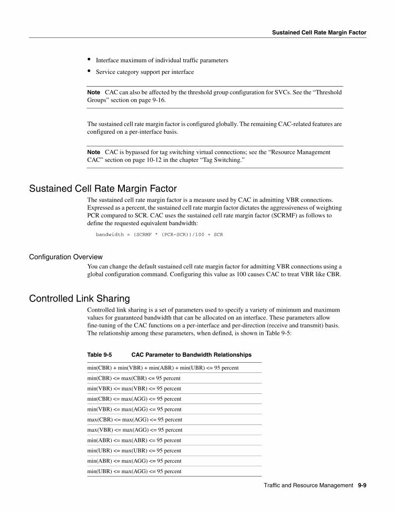
Sustained Cell Rate Margin Factor
• Interface maximum of individual traffic parameters
• Service category support per interface
Note CAC can also be affected by the threshold group configuration for SVCs. See the “Threshold Groups” section on page 9-16.
The sustained cell rate margin factor is configured globally. The remaining CAC-related features are configured on a per-interface basis.
Note CAC is bypassed for tag switching virtual connections; see the “Resource Management CAC” section on page 10-12 in the chapter “Tag Switching.”
Sustained Cell Rate Margin FactorThe sustained cell rate margin factor is a measure used by CAC in admitting VBR connections. Expressed as a percent, the sustained cell rate margin factor dictates the aggressiveness of weighting PCR compared to SCR. CAC uses the sustained cell rate margin factor (SCRMF) as follows to define the requested equivalent bandwidth:
bandwidth = (SCRMF * (PCR-SCR))/100 + SCR
Configuration OverviewYou can change the default sustained cell rate margin factor for admitting VBR connections using a global configuration command. Configuring this value as 100 causes CAC to treat VBR like CBR.
Controlled Link Sharing Controlled link sharing is a set of parameters used to specify a variety of minimum and maximum values for guaranteed bandwidth that can be allocated on an interface. These parameters allow fine-tuning of the CAC functions on a per-interface and per-direction (receive and transmit) basis. The relationship among these parameters, when defined, is shown in Table 9-5:
Table 9-5 CAC Parameter to Bandwidth Relationships
min(CBR) + min(VBR) + min(ABR) + min(UBR) <= 95 percent
min(CBR) <= max(CBR) <= 95 percent
min(VBR) <= max(VBR) <= 95 percent
min(CBR) <= max(AGG) <= 95 percent
min(VBR) <= max(AGG) <= 95 percent
max(CBR) <= max(AGG) <= 95 percent
max(VBR) <= max(AGG) <= 95 percent
min(ABR) <= max(ABR) <= 95 percent
min(UBR) <= max(UBR) <= 95 percent
min(ABR) <= max(AGG) <= 95 percent
min(UBR) <= max(AGG) <= 95 percent
Traffic and Resource Management 9-9
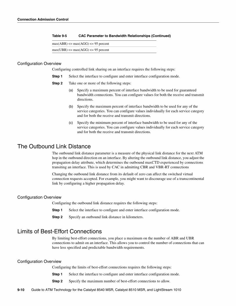
Connection Admission Control
Configuration OverviewConfiguring controlled link sharing on an interface requires the following steps:
Step 1 Select the interface to configure and enter interface configuration mode.
Step 2 Take one or more of the following steps:
(a) Specify a maximum percent of interface bandwidth to be used for guaranteed bandwidth connections. You can configure values for both the receive and transmit directions.
(b) Specify the maximum percent of interface bandwidth to be used for any of the service categories. You can configure values individually for each service category and for both the receive and transmit directions.
(c) Specify the minimum percent of interface bandwidth to be used for any of the service categories. You can configure values individually for each service category and for both the receive and transmit directions.
The Outbound Link DistanceThe outbound link distance parameter is a measure of the physical link distance for the next ATM hop in the outbound direction on an interface. By altering the outbound link distance, you adjust the propagation delay attribute, which determines the outbound maxCTD experienced by connections transiting an interface. This is used by CAC in admitting CBR and VBR-RT connections
Changing the outbound link distance from its default of zero can affect the switched virtual connection requests accepted. For example, you might want to discourage use of a transcontinental link by configuring a higher propagation delay.
Configuration OverviewConfiguring the outbound link distance requires the following steps:
Step 1 Select the interface to configure and enter interface configuration mode.
Step 2 Specify an outbound link distance in kilometers.
Limits of Best-Effort ConnectionsBy limiting best-effort connections, you place a maximum on the number of ABR and UBR connections to admit on an interface. This allows you to control the number of connections that can have less specified and predictable bandwidth requirements.
Configuration OverviewConfiguring the limits of best-effort connections requires the following steps:
Step 1 Select the interface to configure and enter interface configuration mode.
Step 2 Specify the maximum number of best-effort connections to allow.
max(ABR) <= max(AGG) <= 95 percent
max(UBR) <= max(AGG) <= 95 percent
Table 9-5 CAC Parameter to Bandwidth Relationships (Continued)
Guide to ATM Technology for the Catalyst 8540 MSR, Catalyst 8510 MSR, and LightStream 10109-10
Maximum of Individual Traffic Parameters
Maximum of Individual Traffic Parameters You can set maximum values for traffic parameters that are allowed by CAC. Connection requests that exceed the configured maximums on the interface are refused. These traffic parameter limits can be configured independently by service category and traffic direction (receive and transmit). You can specify maximum values for PCR, SCR, MCR, CDVT, and MBS.
Configuration OverviewConfiguring the maximum traffic parameters on an interface requires the following steps:
Step 1 Select the interface to configure and enter interface configuration mode.
Step 2 Do one or more of the following steps for the receive direction, transmit direction, or both, on the interface:
(a) Specify a maximum PCR value in Kbps for any of the CBR, VBR, ABR, and UBR service categories.
(b) Specify a maximum SCR value in Kbps.
(c) Specify a maximum CDVT value (expressed in 2.72 microsecond cell times) for any of the CBR, VBR, ABR, and UBR service categories.
(d) Specify a maximum MBS value in number of cells.
(e) Specify a maximum MCR value in Kbps for the best-effort service categories (ABR and UBR).
Interface Service Category SupportedThis feature allows you to configure which service categories CAC allows on an interface. It allows you explicitly to permit or deny any of the CBR, VBR-RT, VBR-NRT, ABR, and UBR traffic categories.
Interface service category configuration is supported only on physical interfaces and shaped and hierarchical VP tunnel interfaces. The underlying VP for shaped and hierarchical VP tunnel logical interfaces must use the CBR service category. The default for shaped VP tunnels is to allow only CBR virtual connections to transit the interface. However, interface service category configuration can be used to specify a service category other than CBR for virtual connections within a shaped VP tunnel.
The transit VP—the VP that connects the tunnel across the service provider network—must also have a service category. Table 9-6 shows the service category of the shaped VP tunnel (always CBR), the service categories you can configure for transported virtual connections, and a suggested transit VP service category for the tunnel.
Traffic and Resource Management 9-11
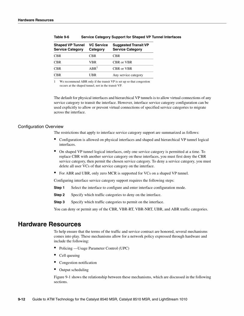
Hardware Resources
Table 9-6 Service Category Support for Shaped VP Tunnel Interfaces
The default for physical interfaces and hierarchical VP tunnels is to allow virtual connections of any service category to transit the interface. However, interface service category configuration can be used explicitly to allow or prevent virtual connections of specified service categories to migrate across the interface.
Configuration OverviewThe restrictions that apply to interface service category support are summarized as follows:
• Configuration is allowed on physical interfaces and shaped and hierarchical VP tunnel logical interfaces.
• On shaped VP tunnel logical interfaces, only one service category is permitted at a time. To replace CBR with another service category on these interfaces, you must first deny the CBR service category, then permit the chosen service category. To deny a service category, you must delete all user VCs of that service category on the interface.
• For ABR and UBR, only zero MCR is supported for VCs on a shaped VP tunnel.
Configuring interface service category support requires the following steps:
Step 1 Select the interface to configure and enter interface configuration mode.
Step 2 Specify which traffic categories to deny on the interface.
Step 3 Specify which traffic categories to permit on the interface.
You can deny or permit any of the CBR, VBR-RT, VBR-NRT, UBR, and ABR traffic categories.
Hardware ResourcesTo help ensure that the terms of the traffic and service contract are honored, several mechanisms comes into play. These mechanisms allow for a network policy expressed through hardware and include the following:
• Policing —Usage Parameter Control (UPC)
• Cell queuing
• Congestion notification
• Output scheduling
Figure 9-1 shows the relationship between these mechanisms, which are discussed in the following sections.
Shaped VP Tunnel Service Category
VC Service Category
Suggested Transit VP Service Category
CBR CBR CBR
CBR VBR CBR or VBR
CBR ABR1
1 We recommend ABR only if the transit VP is set up so that congestion occurs at the shaped tunnel, not in the transit VP.
CBR or VBR
CBR UBR Any service category
Guide to ATM Technology for the Catalyst 8540 MSR, Catalyst 8510 MSR, and LightStream 10109-12

UPC—Traffic Policing at a Network Boundary
Figure 9-1 Traffic Management and Congestion Control Mechanisms
For most applications, when one or more cells are dropped by the network, the corresponding packet becomes corrupted and useless. This results in the need to retransmit the many cells that comprise that packet, and leads to exacerbated congestion. For example, loss of a cell from an IP over ATM packet (RFC 1577) might require resending 192 ATM cells, given an MTU of 9 KB.
To maximize the number of complete delivered packets, the ATM switch router implements a unique tail packet discard and early packet discard (TPD/EPD) scheme that intelligently and selectively discards cells belonging to the same packet. These congestion control mechanisms reduce the effects of fragmentation and make the ATM switch router essentially emulate a packet switch, which discards entire packets.
UPC—Traffic Policing at a Network BoundaryTraffic policing, called UPC by the ATM Forum, monitors and controls the traffic on an ATM connection in terms of cell traffic volume and cell routing validity. The main purpose of UPC is to protect the network resources from abusive connections and to enforce the compliance of a connection to its negotiated traffic contract. UPC is implemented on the ATM switch router in conformance with the ATM Forum Generic Cell Rate Algorithm (GCRA).
UPC on the ATM switch router checks the following parameters:
• PCR and CDVT for CBR, UBR, and ABR connections
• SCR and MBS for VBR connections
On systems equipped with hardware to support the dual leaky bucket, there are two policers for VBR connections. One policer uses PCR and CDVT, while the other policer uses SCR and MBS.
Policing Actions and MechanismsWhen a cell is found to be nonconforming, one of the following actions can be triggered:
• Pass—the cell is untouched.
• Tag—the CLP bit is set in the cell header, tagging the cell for dropping before higher-priority cells.
• Drop—the cell is dropped.
UPC
CLPdiscard
Packetdiscard
Scheduler/shaping
2507
4
Maxqueuelimits
EFCImarking
Cellqueuing
Traffic and Resource Management 9-13

Hardware Resources
CLPThe CLP bit in the ATM cell header can be used to generate different priority cell flows within a virtual connection. When UPC sets CLP = 1, the cell is more likely to experience loss during congestion. This allows a selective cell discarding scheme to be implemented to deal with network congestion.
Per-VC and per-VP UPC BehaviorThe default UPC behavior is to pass nonconforming cells. You can configure UPC to pass or tag PVCs, PVPs, and SVCs.
Configuration OverviewConfiguring the default UPC behavior requires the following steps:
Step 1 For permanent virtual connections, specify UPC tag or drop in the command when you configure the PVC or PVP; the behavior for each half-leg of the connection can be separately configured.
Step 2 For SVCs, select an interface, enter interface configuration mode, and specify tag or drop.
Default CDVT and MBSYou can change the default CDVT and MBS for UPC of cells received on the interface for connections that do not individually request a CDVT or MBS value.
You can specify CDVT or MBS for PVCs through a connection traffic table row. If no CDVT or MBS is specified in the row, then a per-interface, per-service category default is applied for purposes of UPC on the connection.
Note CDVT cannot be signaled. Therefore, the defaults specified on the interface apply for SVCs and the destination leg of a soft PVC.
Configuration OverviewConfiguring the default CDVT and MBS on an interface requires the following steps:
Step 1 Select the interface to configure and enter interface configuration mode.
Step 2 Specify a CDVT default value for a service category. You can repeat this step for additional service categories you want to configure.
Step 3 Specify an MBS default value for a service category. You can repeat this step for additional service categories you want to configure.
Guide to ATM Technology for the Catalyst 8540 MSR, Catalyst 8510 MSR, and LightStream 10109-14

Cell Queuing
Cell QueuingThe ATM switch router allows for flexible control of queueing through configurable queue limits and thresholds.
The specific features available depend upon the hardware:
• For systems with the FC-PCQ
— Oversubscription factor
— Service category limit
— Maximum queue size per interface
— Interface queue thresholds per service category
• For systems with the FC-PFQ and the Catalyst 8540 MSR, threshold groups can be configured.
Oversubscription FactorThe switch oversubscription factor is used in determining initial port maximum queue size for VBR-NRT and ABR/UBR queues.
The size of the VBR-NRT queue and ABR/UBR queues is determined by using the oversubscription factor (OSF) in the following formula:
size (vbr-nrt) = .25 * ((osf * 2048) - DefaultSize (cbr) - DefaultSize (vbr-rt))size (abr-ubr) = .75 * ((osf * 2048) - DefaultSize (cbr) - DefaultSize (vbr-rt))
When you configure the oversubscription factor, you are changing the default values. Refer to the ATM Switch Router Command Reference publication for details.
Configuration OverviewConfiguring the oversubscription factor requires the following steps:
Step 1 From global configuration mode, specify a value for the oversubscription factor.
Step 2 To have the change take effect and resize the queues, save the running configuration to the startup configuration and restart the ATM switch router.
Service Category LimitThe service category limit configuration restricts the number of cells admitted into the switch by output queue type. Limits can be specified for CBR, VBR-RT, VBR-NRT, and ABR/UBR queues.
When you configure the service category limit requirements, you are specifying a new value to use rather than the default. To do so requires just one global configuration command in which you specify the limit in number of cells for a queue type. You repeat this command for each additional queue type for which you want to configure a maximum.
Maximum Queue Size Per InterfaceThe maximum queue size per interface is used to determine the maximum number of cells in the switch fabric queue. This also implicitly affects maxCTD and ppCDV on an output interface. The values set for VBR-RT and ABR/UBR override any set with the oversubscription factor feature.
Traffic and Resource Management 9-15

Hardware Resources
Configuration OverviewConfiguring the maximum queue size for an interface requires the following steps:
Step 1 Select the interface to configure and enter interface configuration mode.
Step 2 Specify an output queue maximum size for a service category. Repeat for additional service categories you want to configure.
Interface Queue Thresholds Per Service CategoryThe queue thresholds can be configured for the service categories on each interface queue.
The following queue thresholds can be configured per interface queue:
• Threshold at which the EFCI bit is set
• Threshold at which cells are eligible for CLP discard or EPD
• Threshold for relative rate (RR) marking on ABR connections
Configuration OverviewConfiguring the interface queue threshold per service category requires the following steps:
Step 1 Select the interface to configure and enter interface configuration mode.
Step 2 Specify an output percent for the EFCI marking threshold for a service category. You can repeat this step for additional service categories on the interface.
Step 3 Specify an output percent for the discard threshold for a service category. You can repeat this step for additional service categories on the interface.
Step 4 Specify an output threshold percent for RR marking on ABR connections.
Threshold GroupsA threshold group utilizes the memory efficiently among virtual connections of a particular traffic type. By default, each threshold group is programmed with a dynamic memory allocation profile that maps into the needs of the connections of a particular service class, and all the connections in a particular service category map into one threshold group.
Note The threshold groups feature depends upon the hardware model and feature card installed in the ATM switch router. In addition, the total number of threshold groups available on the ATM switch router is platform dependent. For details, refer to the ATM Switch Router Software Configuration Guide.
Each threshold group has a set of eight regions, and each region has a set of thresholds. When these thresholds are exceeded, cells are dropped to maintain the integrity of the shared memory resource.
Guide to ATM Technology for the Catalyst 8540 MSR, Catalyst 8510 MSR, and LightStream 10109-16

Cell Queuing
Threshold Group DefaultsThe initial default configuration of per-VC queuing on the ATM switch router has all the connections of a service category assigned to one threshold group. However, the assignment of service categories to threshold groups is configurable, with the following restrictions:
• A service category cannot be mapped to more than one threshold group.
• If you configure a service category to a threshold group more than once, only the last configuration is in effect.
• The default assigns each service category to a different threshold group. However, you can assign more than one service category to a threshold group.
Note The configuration of threshold groups is static, not dynamic.
The threshold group configuration parameters are as follows:
Table 9-7 Threshold Group Defaults
How It WorksAs a threshold group congests (the cumulative number of cells on the queues of virtual connections in the threshold group approaches the configured max-cells value), the maximum number of cells per-queue shrinks from the threshold group max-queue-limit to min-queue-limit.
Note If the max- and min-queue-limits are equal, the queue size does not reduce as the group congests.
When congestion is in the range of 0 cells (uncongested) to 1/8th full, the connection queues are limited to max-queue-size. When congestion is in the range of 7/8ths full to completely full, the connection queues are limited to min-queue-size.
Configuration OverviewConfiguring the threshold group parameters requires the following steps:
Step 1 From global configuration mode, assign a service category to a threshold group (1-6).
Step 2 Specify the maximum number of cells queued for all connections that are members of the threshold group.
GroupMaximum Cells
Maximum Queue Limit
Minimum Queue Limit
Mark Threshold
Discard Threshold Use
1 65535 63 63 25% 87% CBR
2 65535 127 127 25% 87% VBR-RT
3 65535 511 31 25% 87% VBR-NRT
4 65535 511 31 25% 87% ABR
5 65535 511 31 25% 87% UBR
6 65535 1023 1023 25% 87% well-known VCs
Traffic and Resource Management 9-17

Hardware Resources
Step 3 Specify the percent at which the per-connection queue is to be considered full for purposes of CLP discard and EPD.
Step 4 Specify the maximum per-connection queue limit (in number of cells) for the threshold group.
Step 5 Specify the minimum per-connection queue limit (in number of cells) for the threshold group.
Step 6 Specify a name to associate with the threshold group (optional).
Step 7 Specify the percent at which the per-connection queue is considered full for EFCI (on all connections) and RR marking (on ABR connections).
Note RR marking is not supported on all platforms.
You can repeat these steps for any additional service category thresholds you want to configure.
Congestion NotificationThe ATM switch router implements two methods to indicate and control congestion:
• EFCI marking (for non-ABR connections)—In this mode the ATM switch router sets the EFCI state in the headers of forward data cells to indicate congestion. When the destination receives an EFCI flag, it marks the congestion indication bit in the resource management cells to indicate congestion and sends the resource management cells back to the destination.
• Relative rate (RR) marking mode (for ABR connections)—In this mode an ATM switch router that experiences congestion can set the congestion indication bit directly in forward and backward resource management cells. RR marking mode is used only for ABR connections and is not supported on all hardware platforms.
EFCI and RR marking involve two important functions: detecting incipient congestion and providing selective feedback to the source. As with any feedback mechanism, congestion control schemes operate best when the latency of the feedback path is minimized. Thus RR mode, because of its ability to use backward RM cells to send the congestion indicator rather than relying on the destination end system to reflect it back, can greatly reduce feedback delays and deliver better performance than the EFCI mode.
The two modes can be used independently or in combination to support ABR traffic, and thresholds can be set to indicate when EFCI or RR marking should occur.
ABR Congestion Notification ModeThe ABR congestion notification mode is used to change the type of notification used on ABR connections to alert the end station of congestion. ABR mode configuration determines whether ABR uses EFCI marking, RR marking, or both, for forward and backward RM cells used to control ABR congestion. On systems that support RR mode, the ATM switch router uses that mode by default.
Note The ABR congestion notification mode feature depends upon the feature card installed in the ATM switch router. Systems that do not support this feature use only the EFCI mode.
Guide to ATM Technology for the Catalyst 8540 MSR, Catalyst 8510 MSR, and LightStream 10109-18

Output Scheduling
Configuration OverviewWhen you configure the ABR congestion notification mode you affect all ABR connections. To do so requires just one global configuration command.
Output SchedulingOutput scheduling determines which queued cell is chosen to be transmitted out an interface during a cell time, which is dependent upon the characteristics of the physical interface. The goal of output scheduling is to ensure that bandwidth guarantees are met and extra bandwidth is fairly shared among connections.
Note No per-VC or per-VP shaping is performed on systems equipped with FC-PCQ. On systems equipped with FC-PFQ, as well as the Catalyst 8540 MSR, all transit CBR VCs and VPs are shaped.
An additional benefit of output scheduling is the ability to shape traffic. This capability can be important when connecting across a public UNI to a public network, because many such networks base their tariffs on the maximum aggregate bandwidth. Traffic shaping and traffic policing are complementary functions, as illustrated in Figure 9-2.
Figure 9-2 Traffic Shaping and Policing
Traffic shaping is a feature of shaped and hierarchical VP tunnels. See the “VP Tunnels” section on page 4-5 in the chapter “ATM Network Interfaces.”
The following configurable features on the ATM switch router are used for output scheduling:
• Interface output pacing (systems with FC-PCQ)
• Scheduler and service class (system with FC-PFQ, and the Catalyst 8540 MSR)
Interface Output PacingOutput pacing is used to artificially reduce the output speed of an interface in Kbps. Output pacing can be changed at any time or enabled or disabled.
Actual data Shaped dataShaping Policing
(UPC)
* Limit peak rate of cells transmitted
Does received trafficmeet contract? If not:
**
Discard cells, orTag cells 25
075
Traffic and Resource Management 9-19

Hardware Resources
Configuration OverviewInterface output pacing is disabled by default on the ATM switch router. Configuring the interface output pacing requires the following steps:
Step 1 Select the interface to configure and enter interface configuration mode.
Note There are restrictions on which interface types can be configured for output pacing; refer to the ATM Switch Router Command Reference publication for details.
Step 2 Specify the output pacing limit as a a bit rate in Kbps.
This configuration does not take effect if the amount of bandwidth allocated to CBR and VBR connections in the transmit direction on the interface is greater than the configured output pacing value.
Scheduler and Service ClassFor purposes of scheduling, up to eight QoS classes (zero to seven) can be allocated to each physical interface port. Each port has an independent logical rate scheduler (RS) and a weighted round robin (WRR) scheduler. The RS guarantees minimum bandwidth and has first priority on supplying an eligible cell for transmission. Second priority is given to the service classes that have been assigned relative weights based on the ratio of the total leftover bandwidth. The service class relative weights are configurable so that you can change the priority of the default values. The virtual connections within a service class also have relative weights. The service classes and virtual connections within a service class are scheduled by the WRR scheduler based on their relative weights.
In scheduling the next cell to be transmitted from a port, RS has first call on supplying an eligible cell. If RS does not have one, then the WRR scheduler chooses a service class with an output virtual connection ready to transmit, and finally a virtual connection within the service class is selected.
Note Scheduler and service class configuration depends upon the feature card installed in the ATM switch router. On systems that do not support scheduler and service class configuration, output scheduling is done on a strict priority basis; refer to the ATM Switch Router Software Configuration Guide for details.
On the ATM switch router, the ATM service categories are mapped statically to service classes, as shown in Table 9-8; service class 2 has the highest scheduling priority.
Table 9-8 ATM Service Category to Service Class
A different set of service classes is used for tag switching VCs; see the “Tag Switching CoS” section on page 10-9 of the chapter “Tag Switching.”
Service Category Service Class
VBR-RT 2
VBR-NRT 3
ABR 4
UBR 5
Guide to ATM Technology for the Catalyst 8540 MSR, Catalyst 8510 MSR, and LightStream 10109-20

Output Scheduling
The first scheduling decision is made based on whether any rate-scheduled cell is ready (as decided by the timewheel rate scheduler for an interface). Whether a virtual connection uses the rate scheduler is not user-configurable.
Table 9-9 lists the cell rates that are guaranteed by the rate scheduler for each service category.
Table 9-9 Rate Scheduler to Service Category
If the timewheel RS does not have an output virtual circuit ready to transmit, the WRR scheduler becomes active to pick out a virtual circuit to transmit a cell. The WRR scheduler uses the interface bandwidth left over after guaranteed cell service to transmit cells. Thus, an output virtual circuit of a service category other than CBR can be serviced by both the rate scheduler and the WRR scheduler. A CBR output virtual circuit cannot be serviced by the WRR scheduler because its PCR is already guaranteed by the rate scheduler. (Any additional cell transmission by the WRR scheduler out of that output virtual circuit is likely to arrive too soon at the next switch and might be policed.)
The following service categories can be serviced by the WRR scheduler:
• VBR-RT
• VBR-NRT
• ABR
• UBR
The combined result of the two schedulers is illustrated in Figure 9-3.
Figure 9-3 Rate and WRR Scheduling of Cells Through an Output Interface
Each service class is assigned a weight. These weights are configurable, in the range of 1 to 15. The default weighting is {15,2,2,2} for classes {2,3,4,5}, respectively. The weighting is not modified dynamically.
Service Category Cell Rate Guaranteed
CBR PCR
VBR-RT SCR
VBR-NRT SCR
ABR nonzero MCR (if specified)
UBR MCR (if specified)
Rate scheduled (RS)
CBR:PCRVBR-RT:SCRVBR-NRT:SCRABR:MCRUBR:MCR
Weighted round-robin (WRR) scheduled
Highest priority
Lowest priority
Priority ofcells scheduled
S67
85
Traffic and Resource Management 9-21

Hardware Resources
Within service classes, individual output virtual circuits are also weighted, again in the range of 1 to 15. A standard weight (2) is assigned to all PVCs in a service class. Optionally, permanent virtual circuits can be configured with a specific weight per half-leg (applying to the transmit output virtual circuit weight). Switched virtual circuits take the value 2.
Configuration OverviewConfiguring the service class weights on an interface requires the following steps:
Step 1 Select the interface to configure and enter interface configuration mode.
Step 2 Specify a service class and a weight value. You can repeat this step for additional service classes.
Guide to ATM Technology for the Catalyst 8540 MSR, Catalyst 8510 MSR, and LightStream 10109-22

78-6275-03
C H A P T E R 11
Tag SwitchingThis chapter describes tag switching, a high-performance, packet-forwarding technology developed by Cisco Systems. Tag switching combines the benefits of routing with the performance of switching.
Note The information in this chapter is applicable to the Catalyst 8540 MSR, Catalyst 8510 MSR, and LightStream 1010 ATM switch routers. For detailed configuration information, refer to the ATM Switch Router Software Configuration Guide and the ATM Switch Router Command Reference publication.
This chapter includes the following sections:
• “Overview” section on page 11-1
• “Tag Switching in ATM Environments” section on page 11-4
• “Hardware and Software Requirements and Restrictions” section on page 11-5
• “General Procedure for Configuring Tag Switching” section on page 11-5
OverviewTag switching, which integrates network layer (Layer 3) routing and data link layer (Layer 2) switching, provides scalable, high-speed switching in the network core. Tag switching technology is based on the concept of label swapping, in which packets or cells are assigned short, fixed-length labels that tell switching nodes how data should be forwarded.
Tag switching provides additional benefits in the areas of functionality, scalability, traffic management, and flexibility for service providers. For example, tag switching offers a flexible and scalable method to provide virtual private network (VPN) services with QoS. The traffic engineering features of tag switching are useful for managing traffic and link utilization in a routed network. Finally, tag switching’s ability to integrate ATM and IP technology is of interest to those who want to use an ATM backbone to build a multiservice network.
The Internet Engineering Task Force (IETF) is developing a standard for tag switching based on Cisco’s technology. The IETF term for its tag switching standard is Multiprotocol Label Switching (MPLS).
1-1Guide to ATM Technology

R
Chapter 1 ATM Technology FundamentalsCommon Physical Interface Types
Tag Switching ComponentsA tag switching network consists of two types of devices, tag edge routers and tag switches (see Figure 11-1).
Figure 11-1 Tag Switching Network
Tag Edge Routers
Tag edge routers are network layer routing devices located at the edges of a tag switching network. Tag edge routers examine packets entering the tag switching network and apply the proper tag, or label, to the packet before forwarding it to the next hop. For packets leaving the tag switching network, tag edge routers perform the reverse function, removing tags from packets. Tag edge routers also perform value-added network layer services such as security, accounting, and QoS classification.
Tag edge routers use standard routing protocols to create routing tables, which identify routes through the network. Based on the routing tables, tag edge routers use the Tag Distribution Protocol (TDP) to apply and distribute tags to other tag edge routers or tag switches.
Tag Switches
At the core of a tag switching network are tag switches, which forward tagged packets or cells based on tags. ATM switches can be used as tag switches, allowing lookup and forwarding capabilities using fast hardware techniques. Because tag switching and ATM Forum-compliant ATM can coexist on the same ATM switch, your ATM switch router can provide both tag switching and ATM services in parallel. Standard routers, equipped with the proper software, can also function as tag switches.
Tag switches receive TDP information from the tag edge routers and build their own forwarding database. Tag switches then switch the packets based on the tags only (VPI/VCI in the case of ATM), without looking at the Layer 3 header.
Tag Distribution Protocol
The Tag Distribution Protocol (TDP) is used by tag switching devices to distribute, request, and release tag binding information for the IP protocol in a tag switching network. TDP does not replace a routing protocol. Instead, it uses information learned from the routing protocol to create tag bindings.
S67
76
Tag switch (ATMswitch or router)
Tag edge router
unning H/F 4#Guide to ATM Technology
78-6275-03

Chapter 1 ATM Technology FundamentalsCommon Physical Interface Types
Information Components
Tag switching utilizes three types of information bases for storing and retrieving forwarding information:
• Forwarding Information Base (FIB)—a condensed form of routing table containing the destination address, next-hop address, and outgoing interface. Routers make forwarding decisions based on the destination address of a packet plus the information in the FIB.
• Tag Information Base (TIB)—serves to bind an incoming tag to one or more of the following:
– Outgoing tag
– Destination address
– Outgoing link-level information
A TIB can exist for a whole switch, an interface, or a combination of the two.
• Tag Forwarding Information Base (TFIB)—uses information from the FIB and TIB to construct the forwarding information, consisting of the incoming interface, destination address, incoming tag, most efficient next hop, and outgoing interface.
How It WorksIn conventional Layer 3 forwarding, as a packet traverses the network, each router extracts forwarding information from the Layer 3 header. Header analysis is repeated at each router (hop) through which the packet passes.
In a tag switching network, the Layer 3 header is analyzed just once. It is then mapped into a short fixed-length tag. At each hop, the forwarding decision is made by looking only at the value of the tag. There is no need to reanalyze the Layer 3 header. Because the tag is a fixed-length, unstructured value, lookup is fast and simple.
Figure 11-2 illustrates the operation of a tag switching network.
Figure 11-2 Tag Switching Operation
2460
4
= Tag Distribution Protocol (TDP)
1 & 3 2 & 4 5
1-15Guide to ATM Technology
78-6275-03

R
Chapter 1 ATM Technology FundamentalsCommon Physical Interface Types
When a tag edge router at the entry point of a tag switching network receives a packet for forwarding, the following process occurs:
1. Tag edge routers and tag switches use standard routing protocols to identify routes through the network. This routing information is summarized in the FIB.
2. Tag switches use the tables generated by the standard routing protocols to assign and distribute tag information using TDP. Tag switches receive TDP information and build the TFIB that makes use of the tags.
3. When a tag edge router receives a packet for forwarding across the network, it does the following:
a. Analyzes the network-layer header
b. Performs applicable network-layer services
c. Selects a route for the packet from its routing tables
d. Applies a tag and forwards the packet to the next-hop tag switch
4. The tag switch receives the tagged packet and switches the packet based solely on the tag, without reanalyzing the network-layer header.
5. The packet reaches the tag edge router at the egress point of the network, where the tag is stripped off and the packet delivered.
Tag Switching in ATM EnvironmentsBecause both tag switching and ATM switching forward traffic are based on label swapping, tag switching can readily be applied to ATM switching environments. In addition, ATM switches can use tag switching and still perform ATM Forum standard User-to-Network (UNI) signaling and Private Network-to-Network (PNNI) routing functions.
Advantages
Advantages of implementing tag switching in an ATM network include the following:
• Combines the performance and traffic management capabilities of Layer 2 (data link layer) switching with the scalability and flexibility of Layer 3 (network layer) routing. You can direct packet flows across a router-based network along predetermined paths, such as virtual connections, rather than hop-by-hop as in a typical router-based network. This allows routers to perform advanced traffic management tasks, such as load balancing, in ATM switch routers.
• Uses standard routing protocols and TDP to distribute tag values with other tag switches and with tag edge routers. Unlike standard ATM, there is no call setup procedure.
• There is no need to use switched virtual connections (SVCs) for dynamic IP packet flows. This frees CPU processing power for PNNI and UNI flows, which can be reserved for transferring real-time voice and video and other time-sensitive traffic.
• Implementing tag switching on an ATM switch does not preclude the ability to support an ATM control plane, such as PNNI, on the same switch. On physical interfaces on the ATM switch router, tag switching and the ATM control plane operate in a ships in the night (SIN) mode and are unaware of each other.
• There are no high call setup rates. Standard ATM uses a connection setup procedure to allocate VCIs and program the ATM switching hardware, but tag switching uses standard routing protocols and TDP.
unning H/F 4#Guide to ATM Technology
78-6275-03

Chapter 1 ATM Technology FundamentalsCommon Physical Interface Types
• ATM switches appear as routers to adjacent routers. This provides a scalable alternative to the overlay model (ATM switches in the core network and routers on the periphery) and removes the necessity for ATM addressing, routing, and signaling schemes.
• ATM switches can participate fully in hierarchical routing protocols and act as peers to tag edge routers. Thus the tag edge routers see far fewer peers than if the edge routers were interconnected via virtual connections over the ATM network. Therefore, in terms of the number of network devices, the network can scale to much larger sizes.
Limitations
Limitations of tag switching include the following:
• Only the Open Shortest Path First (OSPF) routing protocol is supported in the tag switching implementation on the ATM switch router.
• Understanding tag switching at the troubleshooting level requires a knowledge of OSPF, the Border Gateway Protocol (BGP), and Cisco Express Forwarding (CEF).
Hardware and Software Requirements and RestrictionsTag switching has certain hardware requirements on the ATM switch router. For specifics, refer to the ATM Switch Router Software Configuration Guide.
Tag switching on the ATM switch router has the following software restrictions:
• OSPF is the only routing protocol currently supported.
• IP is the only network layer protocol supported.
• Hierarchical VP tunnels and tag switching cannot co-exist on a physical interface.
• No tag switching virtual connections (or any other virtual connections) can be set up on a physical interface with a hierarchical VP tunnel.
General Procedure for Configuring Tag SwitchingThis section provides a high-level overview of configuring tag switching on ATM switch routers. Following is a summary of the tasks:
Step 1 Configure a loopback interface.
Step 2 Enable tag switching on the ATM interface.
Step 3 Configure OSPF.
Step 4 Configure a VPI range (optional).
Step 5 Configure TDP control channel (optional).
Step 6 Configure tag switching on VP tunnels.
Step 7 Configure VC merge (optional).
Step 8 Configure CoS.
1-15Guide to ATM Technology
78-6275-03

R
Chapter 1 ATM Technology FundamentalsCommon Physical Interface Types
The Loopback InterfaceYou should configure a loopback interface on every ATM switch router configured for tag switching. The loopback interface, a virtual interface, is always active. The IP address of the loopback interface is used as the TDP identifier for the ATM switch router. If a loopback interface does not exist, the TDP identifier is the highest IP address configured on the ATM switch router. If that IP address is administratively shut down, all TDP sessions through the ATM switch router restart. Therefore, we recommend that you configure a loopback interface.
Configuring the loopback interface requires the following steps:
Step 1 Enter interface configuration mode and assign a number to the loopback interface.
Step 2 Assign an IP address and subnet mask to the loopback interface.
Tag Switching on the ATM InterfaceEnabling tag switching on the ATM interface requires the following steps:
Step 1 Select the ATM interface to configure and enter interface configuration mode.
Step 2 Do one of the following:
a. Enable IP unnumbered on the ATM interface and assign the unnumbered interface to an interface that has an IP address. This is the recommended method. It allows you to conserve IP addresses and reduces the number of tag virtual channels (TVCs) terminating on the switch.
b. Assign an IP address and subnet mask to the ATM interface.
All parallel interfaces between ATM switch routers should be configured with the same method.
Step 3 Enable tag switching of IPv4 packets on the interface.
The Routing ProtocolOSPF must be enabled on the ATM switch router so that it can create the routing tables used to identify routes through the network. Addresses and associated routing areas are then added to the OSPF process so that it can propagate the addresses to other ATM switch routers.
Configuring OSPF requires the following steps:
Step 1 Enable OSPF and assign it a process number.
Step 2 Define the network prefix, a wildcard subnet mask, and the associated area number on which to run OSPF.
Repeat this step for each additional area you want to add to the OSPF process.
unning H/F 4#Guide to ATM Technology
78-6275-03

Chapter 1 ATM Technology FundamentalsCommon Physical Interface Types
The VPI RangeYou might need to change the default tag virtual path identifier (VPI) range on the switch if:
• It is an administrative policy to use a VPI value other than 1, the default VPI.
• There is a large number of TVCs on an interface.
For an overview of configuring VPI ranges, refer to the “VPI/VCI Ranges for SVCs” section on page 4-11.
Note You cannot enter a VPI range on a VP tunnel. On VP tunnels, the VPI is the permanent virtual path (PVP) number (subinterface number) of the tunnel.
The TDP Control ChannelYou can change the default TDP control channel VPI and VCI if you want to use a nondefault value. The default TDP control channel is on VPI 0 and VCI 32. TDP control channels exchange TDP HELLOs and Protocol Information Elements (PIEs) to establish two-way TDP sessions. TVCs are created by exchanging PIEs through TDP control channels.
Figure 11-3 shows an example TDP control channel configuration between a source switch and destination switch on ATM interface 0/0/1. Note that the VPI and VCI values match on the source switch and destination switch.
Figure 11-3 Configuring TDP Control Channels
Changing the TDP control channel requires the following steps:
Step 1 Select the interface to configure and enter interface configuration mode.
Step 2 Specify the new VPI and VCI values for the new TDP control channel configuration.
Tag Switching on VP TunnelsYou can configure tag switching on VP tunnels. To do so, you must first configure the VP tunnel on the source and destination switch, then connect the VP tunnel at the intermediate switch. VP tunnels are described in the “VP Tunnels” section on page 4-13.
VPI = 6VCI = 32
VPI = 6VCI = 32
0/0/1
Source switch Destination switch
S68
06
1-15Guide to ATM Technology
78-6275-03

R
Chapter 1 ATM Technology FundamentalsCommon Physical Interface Types
Figure 11-4 shows an example VP tunnel between a source switch and destination switch.
Figure 11-4 Configuring VP Tunnels
Configuring tag switching on a VP tunnel requires the following steps:
Step 1 Select the interface to configure and enter interface configuration mode.
Step 2 Create a PVP with a VPI value.
Step 3 Select the interface and subinterface you specified in the previous steps.
Step 4 Enable IP unnumbered or assign an IP address and subnet mask to the subinterface, as described inStep 2 in the “Tag Switching on the ATM Interface” section on page 11-6.
Step 5 Enable tag switching of IPv4 packets on the interface.
Repeat these steps on the ATM switch router at the other end of the VP tunnel.
To complete the VP tunnel, you must configure the ATM ports on the intermediate switch to designate where to send packets coming from the source switch and going to the destination switch.
Figure 11-5 shows an example configuration on an intermediate switch.
Figure 11-5 Connecting the VP Tunnels
Configuring the cross-connect in the intermediate switch requires the following steps:
Step 1 Select one of the interfaces and enter interface configuration mode.
Step 2 Connect the PVP from the source switch to the destination switch by specifying the PVP on this interface, the number of the opposite interface, and the PVP to use on that end.
VC MergeVirtual connection (VC) merge allows the switch to aggregate multiple incoming flows with the same destination address into a single outgoing flow. Where VC merge occurs, several incoming tags are mapped to one single outgoing tag. Cells from different VCIs going to the same destination are
0/1/1 0/1/3
Intermediate switch
PVP 51 PVP 101
Source switch Destination switch
S68
07
0/1/1 PVP 51 PVP 101 0/1/3
Source switch Intermediate switch Destination switch
S68
08
unning H/F 4#Guide to ATM Technology
78-6275-03
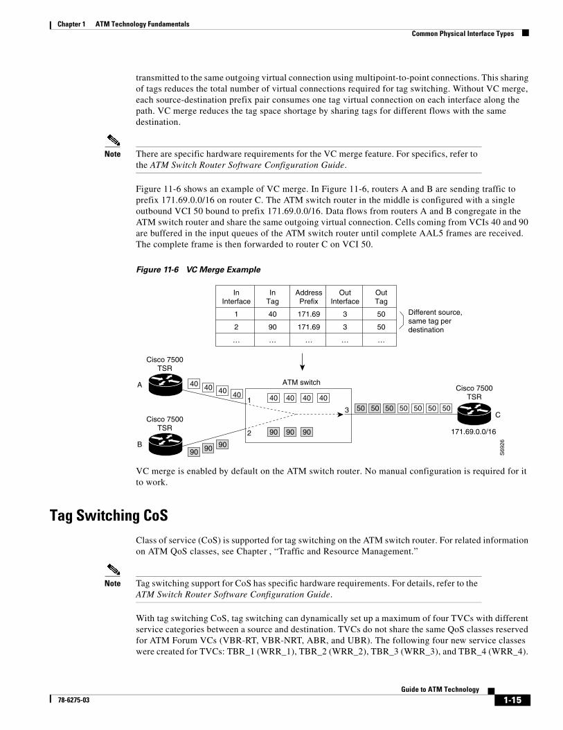
Chapter 1 ATM Technology FundamentalsCommon Physical Interface Types
transmitted to the same outgoing virtual connection using multipoint-to-point connections. This sharing of tags reduces the total number of virtual connections required for tag switching. Without VC merge, each source-destination prefix pair consumes one tag virtual connection on each interface along the path. VC merge reduces the tag space shortage by sharing tags for different flows with the same destination.
Note There are specific hardware requirements for the VC merge feature. For specifics, refer to the ATM Switch Router Software Configuration Guide.
Figure 11-6 shows an example of VC merge. In Figure 11-6, routers A and B are sending traffic to prefix 171.69.0.0/16 on router C. The ATM switch router in the middle is configured with a single outbound VCI 50 bound to prefix 171.69.0.0/16. Data flows from routers A and B congregate in the ATM switch router and share the same outgoing virtual connection. Cells coming from VCIs 40 and 90 are buffered in the input queues of the ATM switch router until complete AAL5 frames are received. The complete frame is then forwarded to router C on VCI 50.
Figure 11-6 VC Merge Example
VC merge is enabled by default on the ATM switch router. No manual configuration is required for it to work.
Tag Switching CoSClass of service (CoS) is supported for tag switching on the ATM switch router. For related information on ATM QoS classes, see Chapter , “Traffic and Resource Management.”
Note Tag switching support for CoS has specific hardware requirements. For details, refer to the ATM Switch Router Software Configuration Guide.
With tag switching CoS, tag switching can dynamically set up a maximum of four TVCs with different service categories between a source and destination. TVCs do not share the same QoS classes reserved for ATM Forum VCs (VBR-RT, VBR-NRT, ABR, and UBR). The following four new service classes were created for TVCs: TBR_1 (WRR_1), TBR_2 (WRR_2), TBR_3 (WRR_3), and TBR_4 (WRR_4).
InInterface
InTag
AddressPrefix
OutInterface
OutTag
1 40 171.69 3 50
2 90 171.69 3 50
… … … … …
Different source,same tag perdestination
ATM switch
Cisco 7500TSR
Cisco 7500TSR
A
Cisco 7500TSR
B
C50 50 50 50 50 50 50
40
90 90 90
40 40 40 40 40 40
90 90 90
401
2
3
171.69.0.0/16
S69
26
1-15Guide to ATM Technology
78-6275-03

R
Chapter 1 ATM Technology FundamentalsCommon Physical Interface Types
These new service classes are called Tag Bit Rate (TBR) classes. TVCs and ATM Forum VCs can only coexist on the same physical interface, but they operate ships in the night mode (SIN) and are unaware of each other.
TBR classes support only best-effort VCs (similar to the ATM Forum service category UBR); therefore, there is no bandwidth guarantee from the rate scheduler (RS) for TVCs. All of the TVCs fall into one of the four TBR classes, which each carry a different default relative weight. The default values of the relative weights for the four TBR classes are configurable so that you can change the priority of the default values.
Table 11-1 shows the TBR classes and ATM Forum class mappings into the service classes for physical ports.
Note The CBR service category is mapped to service class 2, but all CBR VCs are rate scheduled only, and therefore are not weighted round-robin (WRR) scheduled.
When tag switching is enabled on a hierarchical VP tunnel, the tunnel can only be used for tag switching. Because hierarchical VP tunnels support only four service classes, both TVCs and ATM Forum VCs map to the same service classes. Therefore, both ATM Forum VCs and TVCs cannot coexist in a hierarchical VP tunnel. The relative weights assigned to the service classes depend on which is active (either tag switching or ATM Forum). The class weights change whenever a hierarchical tunnel is toggled between ATM Forum and tag switching. By default, a hierarchical VP tunnel comes up as an ATM Forum port.
Table 11-2 lists the mapping of ATM Forum service categories and TBR classes for hierarchical VP tunnels.
Table 11-1 Service Class to Weight Mapping for Physical Ports
TBR Class Service Class Relative Weight
TBR_1 (WRR_1) 1 1
TBR_2 (WRR_2) 6 2
TBR_3 (WRR_3) 7 3
TBR_4 (WRR_4) 8 4
ATM Forum Service Category Service Class Relative Weight
VBR-RT 2 15
VBR-NRT 3 2
ABR 4 2
UBR 5 2
Table 11-2 Service Class to Weight Mapping for Hierarchical VP Tunnels
TBR Class Service Class Relative Weight
TBR_1 (WRR_1) 1 1
TBR_2 (WRR_2) 2 2
unning H/F 4#Guide to ATM Technology
78-6275-03

Chapter 1 ATM Technology FundamentalsCommon Physical Interface Types
Each service class is assigned a relative weight. These weights are configurable, and range from 1 to 15. Configuring the service class and relative weight requires the following steps:
Step 1 Select the interface to configure and enter interface configuration mode.
Step 2 Enter the service class and relative weight for the interface.
Threshold Group for TBR Classes
A threshold group utilizes the memory efficiently among VCs of a particular traffic type. Each threshold group is programmed with a dynamic memory allocation profile that maps into the needs of the connections of a particular service class.
The number of threshold groups available on the ATM switch router is platform dependent. For details, refer to the ATM Switch Router Software Configuration Guide.
Each threshold group has a set of eight regions, and each region has a set of thresholds. When these thresholds are exceeded, cells are dropped to maintain the integrity of the shared memory resource.
Each ATM Forum service category is mapped into a distinct threshold group. All the connections in a particular service category map into one threshold group. Similarly, all the TBR classes have best effort traffic; the service differentiation comes mainly by assigning different weights. Each of the TBR classes map into four different threshold groups whose parameters are the same as the UBR threshold group.
Table 11-3 shows the threshold group parameters mapped to the connections in all of the TBR classes for the ATM switch router.
TBR_3 (WRR_3) 3 3
TBR_4 (WRR_4) 4 4
ATM Forum Service Category Service Class Relative Weight
VBR-RT 1 15
VBR-NRT 2 2
ABR 3 2
UBR 4 2
Table 11-2 Service Class to Weight Mapping for Hierarchical VP Tunnels (continued)
TBR Class Service Class Relative Weight
Table 11-3 Threshold Group Parameters for TVCs
GroupMaximum Cells
Maximum Queue Limit
Minimum Queue Limit
Mark Threshold
Discard Threshold Use
7 131071 511 31 25% 87% TBR_1 (WRR_1)
8 131071 511 31 25% 87% TBR_2 (WRR_2)
1-15Guide to ATM Technology
78-6275-03

R
Chapter 1 ATM Technology FundamentalsCommon Physical Interface Types
Each threshold group is divided into eight regions. Each region has a set of thresholds which are calculated from the corresponding threshold group parameters given in Table 11-3. The threshold group might be in any one of the regions depending on the fill level (cell occupancy) of that group. And that region is used to derive the set of thresholds which apply to all the connections in that group.
Table 11-4 gives the eight thresholds for threshold groups 6, 7, 8, and 9.
For more information about threshold groups, see the “Threshold Groups” section on page -16.
CTT Rows
A row in the connection traffic table (CTT) is created for each unique combination of traffic parameters. When a TVC is set up in response to a request by tag switching, a CTT row is obtained from the resource manager by passing the traffic parameters which include the service category (TBR_x [WRR_x], where x is 1, 2, 3, or 4). If a match is found for the same set of traffic parameters, the row index is returned; otherwise, a new table is created and the row index of that CTT row is returned. Since all data TVCs use the same traffic parameters, the same CTT row can be used for all TVCs of a particular service category once it is created.
Note There are no user configurable parameters for the CTT with TVCs.
9 131071 511 31 25% 87% TBR_3 (WRR_3)
10 131071 511 31 25% 87% TBR_3 (WRR_4)
Table 11-3 Threshold Group Parameters for TVCs (continued)
GroupMaximum Cells
Maximum Queue Limit
Minimum Queue Limit
Mark Threshold
Discard Threshold Use
Table 11-4 Region Thresholds for Threshold Groups
RegionLowerLimit
UpperLimit
Queue Limit
MarkingThreshold
Discard Threshold
0 0 8191 511 127 447
1 8128 16383 255 63 223
2 16320 24575 127 31 111
3 24512 32767 63 15 63
4 32704 40959 31 15 31
5 40896 49151 31 15 31
6 49088 57343 31 15 31
7 57280 65535 31 15 31
unning H/F 4#Guide to ATM Technology
78-6275-03

Chapter 1 ATM Technology FundamentalsCommon Physical Interface Types
Resource Management CAC
Connection admission control (CAC) is not supported for TVCs. All TVCs are best effort connections; therefore, no bandwidth is guaranteed by the RS. Only the WRR scheduler is used. All of the traffic parameters (PCR, MCR, MBS, CDVT, and SCR) are unspecified. There is no best effort limit, as there is with ATM Forum UBR and ABR connections. CAC is bypassed for TVCs.
1-15Guide to ATM Technology
78-6275-03

R
Chapter 1 ATM Technology FundamentalsCommon Physical Interface Types
unning H/F 4#Guide to ATM Technology
78-6275-03

78-6275-03
C H A P T E R12
Frame Relay to ATM InterworkingFrame Relay to ATM interworking is supported on the ATM switch router using the channelized Frame Relay port adapters. These port adapters facilitate interworking between a Frame Relay network, an ATM network, and network users. Existing Frame Relay users can also migrate to higher bandwidth ATM using channelized Frame Relay port adapters. Additionally, these port adapters extend the ATM network across a wide area over a frame-based serial line or an intervening Frame Relay WAN.
Note The information in this chapter is applicable to the Catalyst 8540 MSR, Catalyst 8510 MSR, and LightStream 1010 ATM switch routers. For detailed configuration information, refer to the ATM Switch Router Software Configuration Guide and the ATM Switch Router Command Reference publication.
The chapter includes the following sections:
• Frame Relay to ATM Interworking Overview, page 12-1
• The Channelized DS3 Frame Relay Port Adapter, page 12-3
• The Channelized E1 Frame Relay Port Adapter, page 12-5
• Frame Relay to ATM Interworking Configuration Overview, page 12-7
• LMI Configuration Overview, page 12-8
• Frame Relay to ATM Resource Management Configuration Overview, page 12-9
• Frame Relay to ATM Virtual Connections Configuration Overview, page 12-12
Note This chapter provides technical background and configuration overview information applicable to the Frame Relay port adapters for the ATM switch router. It does not provide general Frame Relay information.
Frame Relay to ATM Interworking OverviewFrame Relay to ATM interworking allows you to retain your existing Frame Relay services and, as needs expand, migrate to the higher bandwidth capabilities provided by ATM networks. Frame Relay traffic connects across high-speed ATM trunks using two interworking functions (IWFs): network interworking and service interworking.
1-1Guide to ATM Technology

R
Chapter 1 ATM Technology FundamentalsCommon Physical Interface Types
The difference between these two interworking functions is that network interworking provides a transport between two Frame Relay devices, while service interworking provides transparent interworking between ATM devices and Frame Relay devices without either being aware of the technology used at the other end.
The implementation of network interworking and service interworking is specified in procedures jointly agreed upon by the Frame Relay Forum and the ATM Forum (FRF.5 and FRF.8).
Network InterworkingThe network interworking function (network IWF) facilitates transport of Frame Relay user traffic and Frame Relay permanent virtual circuit (PVC) signaling traffic over ATM. Tunneling, multiprotocol encapsulation, and other higher layer procedures are handled just as they would be over leased lines. A network IWF application connects Frame Relay devices over an ATM backbone, as shown in Figure 12-1.
Note In this chapter PVC is used interchangeably to mean permanent virtual circuit (in the context of Frame Relay) and permanent virtual connection (in the context of ATM).
Figure 12-1 Frame Relay to ATM Network Interworking
In the example shown in Figure 12-1, the ATM network could take the place of a leased line to connect the two Frame Relay networks. The network IWF is integrated into the channelized Frame Relay port adapter. This method of connecting Frame Relay networks can provide economic savings when compared to leased lines and offers the improved scalability of ATM at the core.
If a Frame Relay port is connected across an ATM network to an ATM device, network interworking requires that the ATM device recognize that it is connected to an interworking function, such as Frame Relay. The ATM device must then exercise the appropriate service-specific convergence sublayer (SSCS), in this case the Frame Relay SSCS (FR-SSCS).
Service InterworkingThe service interworking function (service IWF) provides a transport between two dissimilar devices, such as Frame Relay and ATM. Unlike network IWF, service IWF does not transport traffic transparently. Rather, it serves as a protocol converter and allows communication between dissimilar devices, as shown in Figure 12-2.
Frame Relayrouter
VCL
ATM switch ATM switch
Frame Relayport adapter
Frame Relayport adapter
1521
8
Frame Relayrouter
Frame Relayrouter
Frame Relaynetwork
ATMnetwork
Frame Relaynetwork
unning H/F 4#Guide to ATM Technology
78-6275-03
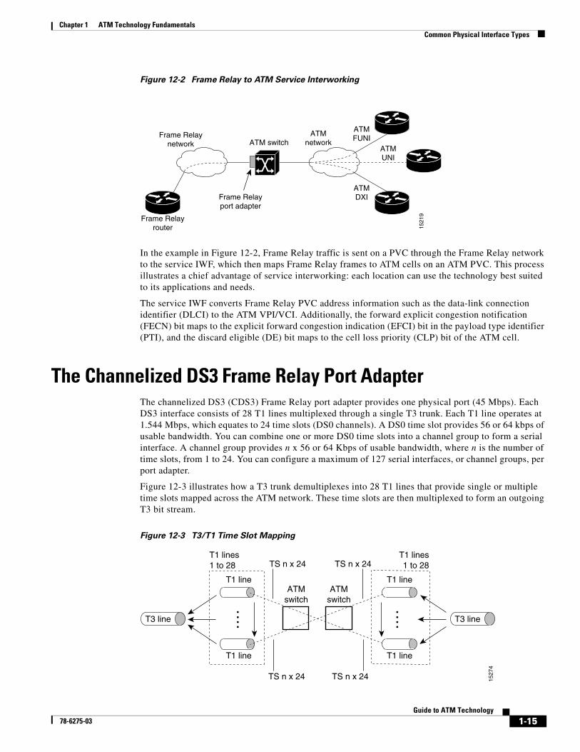
Chapter 1 ATM Technology FundamentalsCommon Physical Interface Types
Figure 12-2 Frame Relay to ATM Service Interworking
In the example in Figure 12-2, Frame Relay traffic is sent on a PVC through the Frame Relay network to the service IWF, which then maps Frame Relay frames to ATM cells on an ATM PVC. This process illustrates a chief advantage of service interworking: each location can use the technology best suited to its applications and needs.
The service IWF converts Frame Relay PVC address information such as the data-link connection identifier (DLCI) to the ATM VPI/VCI. Additionally, the forward explicit congestion notification (FECN) bit maps to the explicit forward congestion indication (EFCI) bit in the payload type identifier (PTI), and the discard eligible (DE) bit maps to the cell loss priority (CLP) bit of the ATM cell.
The Channelized DS3 Frame Relay Port AdapterThe channelized DS3 (CDS3) Frame Relay port adapter provides one physical port (45 Mbps). Each DS3 interface consists of 28 T1 lines multiplexed through a single T3 trunk. Each T1 line operates at 1.544 Mbps, which equates to 24 time slots (DS0 channels). A DS0 time slot provides 56 or 64 kbps of usable bandwidth. You can combine one or more DS0 time slots into a channel group to form a serial interface. A channel group provides n x 56 or 64 Kbps of usable bandwidth, where n is the number of time slots, from 1 to 24. You can configure a maximum of 127 serial interfaces, or channel groups, per port adapter.
Figure 12-3 illustrates how a T3 trunk demultiplexes into 28 T1 lines that provide single or multiple time slots mapped across the ATM network. These time slots are then multiplexed to form an outgoing T3 bit stream.
Figure 12-3 T3/T1 Time Slot Mapping
Frame Relayrouter
VCL
ATM switch
Frame Relayport adapter
1521
9
Frame Relaynetwork
ATMnetwork
ATMFUNI
ATMDXI
ATMUNI
T1 line
T1 line
T3 line
TS n x 24T1 lines1 to 28
T1 lines1 to 28TS n x 24
TS n x 24 TS n x 24
T1 line
T1 line
ATMswitch
ATMswitch
1527
4
T3 line
1-15Guide to ATM Technology
78-6275-03

R
Chapter 1 ATM Technology FundamentalsCommon Physical Interface Types
Configuration GuidelinesTo configure the CDS3 Frame Relay port adapter physical interface, you need the following information:
• Digital transmission link information, for example, T3 and T1 clock source and framing type
• Channel information and time slot mapping
• Protocols and encapsulations you plan to use on the new interfaces
General Procedure for Configuring the CDS3 Frame Relay Port AdapterConfiguring the CDS3 Frame Relay port adapter interface requires the following tasks, described in the following sections:
Step 1 Configure the physical interface.
Step 2 Configure the T1 lines.
Step 3 Configure the channel group.
Physical Interface
The CDS3 Frame Relay port adapter is preconfigured with default values for the physical interface. You can manually change any of the default configuration values by performing the following steps:
Step 1 Enter controller configuration mode and select the CDS3 Frame Relay interface to configure.
Step 2 Specify the clock distribution mode (default is loop-timed). For more information on clocking modes, see Chapter 8, “Network Clock Synchronization.”
Step 3 Specify the DS3 framing type (the default is M23).
Step 4 Specify the cable length (the default is 224).
Step 5 Configure the Maintenance Data Link (MDL) message (the default is no message). MDL messages are only supported when the framing type is set for c-bit parity.
T1 Lines
The CDS3 Frame Relay port adapter is preconfigured with default values for all T1 lines. You can manually change any of the default configuration values by performing the following steps:
Step 1 Enter controller configuration mode and select the CDS3 Frame Relay interface to configure.
Step 2 Specify the T1 framing mode for the lines you are configuring (the default is ESF).
Step 3 Specify T1 yellow alarm detection, generation, or both for the lines you are configuring (the default is both).
unning H/F 4#Guide to ATM Technology
78-6275-03
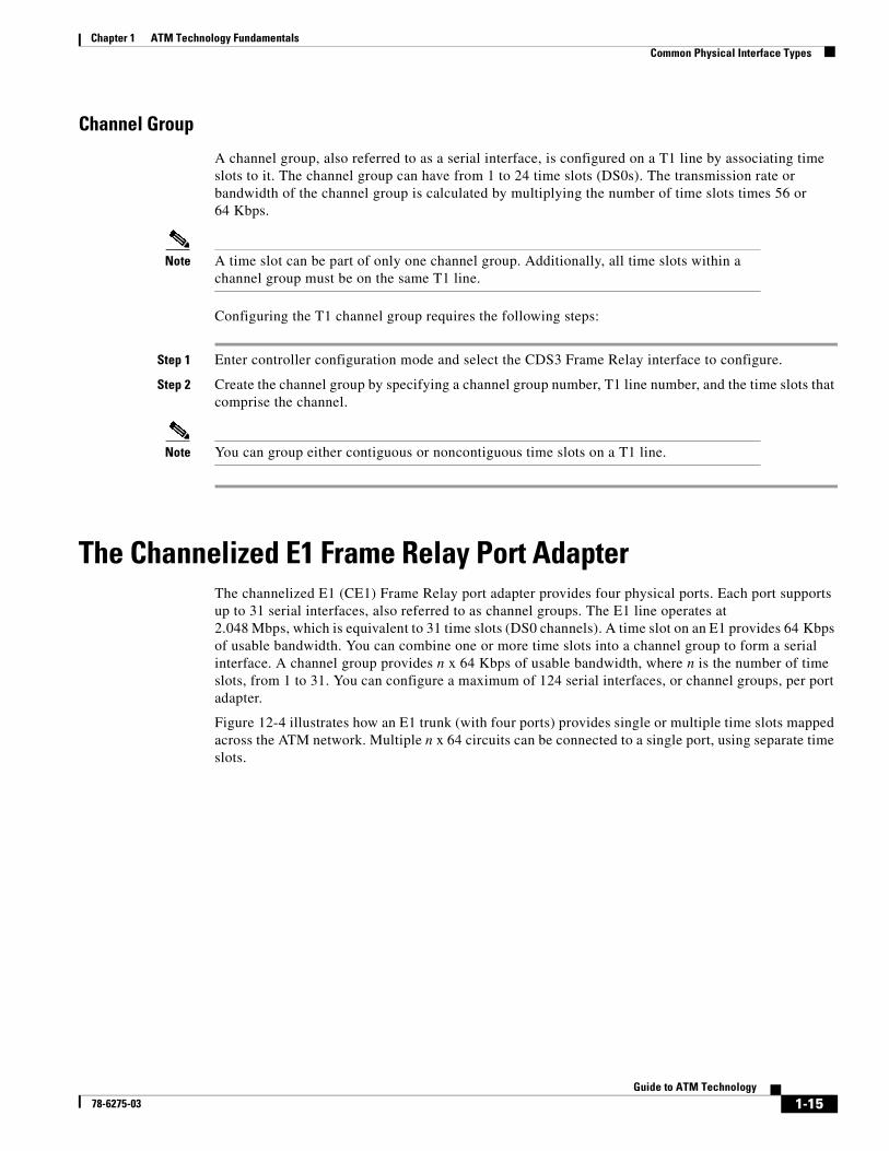
Chapter 1 ATM Technology FundamentalsCommon Physical Interface Types
Channel Group
A channel group, also referred to as a serial interface, is configured on a T1 line by associating time slots to it. The channel group can have from 1 to 24 time slots (DS0s). The transmission rate or bandwidth of the channel group is calculated by multiplying the number of time slots times 56 or 64 Kbps.
Note A time slot can be part of only one channel group. Additionally, all time slots within a channel group must be on the same T1 line.
Configuring the T1 channel group requires the following steps:
Step 1 Enter controller configuration mode and select the CDS3 Frame Relay interface to configure.
Step 2 Create the channel group by specifying a channel group number, T1 line number, and the time slots that comprise the channel.
Note You can group either contiguous or noncontiguous time slots on a T1 line.
The Channelized E1 Frame Relay Port AdapterThe channelized E1 (CE1) Frame Relay port adapter provides four physical ports. Each port supports up to 31 serial interfaces, also referred to as channel groups. The E1 line operates at 2.048 Mbps, which is equivalent to 31 time slots (DS0 channels). A time slot on an E1 provides 64 Kbps of usable bandwidth. You can combine one or more time slots into a channel group to form a serial interface. A channel group provides n x 64 Kbps of usable bandwidth, where n is the number of time slots, from 1 to 31. You can configure a maximum of 124 serial interfaces, or channel groups, per port adapter.
Figure 12-4 illustrates how an E1 trunk (with four ports) provides single or multiple time slots mapped across the ATM network. Multiple n x 64 circuits can be connected to a single port, using separate time slots.
1-15Guide to ATM Technology
78-6275-03

R
Chapter 1 ATM Technology FundamentalsCommon Physical Interface Types
Figure 12-4 E1 Time Slot Mapping
Configuration GuidelinesTo configure the CE1 Frame Relay port adapter, you will need the following information:
• Digital transmission link information, for example, E1 clock source and framing type
• Channel information and time slot mapping
• Protocols and encapsulations you plan to use on the new interfaces
General Procedure for Configuring the CE1 Frame Relay Port AdapterConfiguring the CE1 Frame Relay port adapter interface requires the following tasks, described in the following sections:
Step 1 Configure the physical interface.
Step 2 Configure the channel group.
E1 4 ports
E1 4 ports
E1 4 ports E1 4 ports
E1 4 ports E1 4 ports
(TS 9 x 64)
(TS 12 x 64)
(TS 5 x 64)
(TS 9 x 64) (TS 1 x 64)
(TS 12 x 64) (TS 4 x 64)
(TS 1 x 64) (TS 4 x 64) (TS 5 x 64) (TS 8 x 64)
(TS 8 x 64)
1527
5
ATMswitch
ATMswitch
ATMswitch
unning H/F 4#Guide to ATM Technology
78-6275-03

Chapter 1 ATM Technology FundamentalsCommon Physical Interface Types
The following defaults are assigned to all CE1 Frame Relay port adapter interfaces:
• Framing—crc4
• Clock source—loop-timed
• Linecode—HDB3
Physical Interface
The CE1 Frame Relay port adapter is preconfigured with default values for the physical interface. You can manually change any of the default configuration values by performing the following steps:
Step 1 Enter controller configuration mode and select the CE1 Frame Relay interface to configure.
Step 2 Specify the clock distribution mode (the default is loop-timed). For more information on clocking modes, see Chapter 8, “Network Clock Synchronization.”
Step 3 Specify the DS3 framing type (the default is CRC4).
Channel Group
A channel group, also referred to as a serial interface, is configured on an E1 line by associating time slots to it. The channel group can have from 1 to 31 time slots (DS0s). The transmission rate or bandwidth of the channel group is calculated by multiplying the number of time slots times 64 Kbps.
Configuring the channel group requires the following steps:
Step 1 Enter controller configuration mode and select the CE1 Frame Relay interface to configure.
Step 2 Create the channel group by specifying a channel group number and the time slots that comprise the channel.
Frame Relay to ATM Interworking Configuration OverviewThis section outlines the steps required to enable Frame Relay to ATM interworking on your ATM switch router. In addition, you can customize Frame Relay to ATM for your particular network needs and monitor Frame Relay to ATM connections. Configuring Frame Relay to ATM interworking functions requires the following tasks:
• Enable Frame Relay encapsulation on an interface
• Configure the Frame Relay serial interface type
For information on how to customize your Frame Relay to ATM connections, see the “LMI Configuration Overview” section on page 12-8 and “Frame Relay to ATM Resource Management Configuration Overview” section on page 12-9.
1-15Guide to ATM Technology
78-6275-03
R
Chapter 1 ATM Technology FundamentalsCommon Physical Interface Types
Enable Frame Relay EncapsulationFrame Relay supports encapsulation of all supported protocols in conformance with RFC 1490, allowing interoperability between multiple vendors. Enabling Frame Relay encapsulation on the serial interface requires the following steps:
Step 1 Enter interface configuration mode and select the serial interface to configure.
Step 2 Enable IETF encapsulation on the interface.
Serial Interface TypeYou can configure a serial interface as a data communications equipment (DCE) or Network-to-Network Interface (NNI) type. Configuring the serial interface type requires the following steps:
Step 1 Enter interface configuration mode and select the serial interface to configure.
Step 2 Specify the interface type.
When you specify DCE, the ATM switch router supports only network-side PVC status management procedures. When you specify NNI, the ATM switch router supports both user-side and network-side PVC status management procedures.
LMI Configuration OverviewThe Local Management Interface (LMI) provides a set of enhancements to the basic Frame Relay specification, including support for a keepalive mechanism and statistics. You can configure the following LMI-related parameters on the Frame Relay interface:
• LMI type
• LMI keepalive interval
• LMI polling and timer intervals (optional)
LMI TypeConfiguring the LMI type requires the following steps:
Step 1 Enter interface configuration mode and select the serial interface to configure.
Step 2 Specify a Frame Relay LMI type (Cisco is the default type).
Step 3 Exit configuration mode and save your running configuration to the startup configuration.
unning H/F 4#Guide to ATM Technology
78-6275-03

Chapter 1 ATM Technology FundamentalsCommon Physical Interface Types
LMI Keepalive IntervalA keepalive interval must be set to configure the LMI. By default, this interval is 10 seconds and, per the LMI protocol, must be set as a positive integer that is less than the lmi-t392dce interval set on the interface of the neighboring switch.
Configuring the keepalive interval requires the following steps:
Step 1 Enter interface configuration mode and select the serial interface to configure.
Step 2 Specify a keepalive interface for the interface.
LMI Polling and Timer IntervalsYou can set various optional counters, intervals, and thresholds to fine-tune the operation of your LMI on your Frame Relay devices. Configuring these attributes requires the following steps:
Step 1 Enter interface configuration mode and select the serial interface to configure.
Step 2 Perform one or more of the following substeps:
a. Specify the number of keepalive exchanges to be completed before requesting a full status message.
b. Specify the error threshold for DCE and NNI interfaces.
c. Specify the error threshold for DTE and NNI interfaces.
d. Specify the monitored events count on DCE and NNI interfaces.
e. Specify the monitored event count on DTE and NNI interfaces.
f. Specify the polling verification timer on DCE and NNI interfaces.
Frame Relay to ATM Resource Management Configuration Overview
This section describes the connection traffic table (CTT) rows used specifically for Frame Relay to ATM interworking, and provides an overview of configuring the following features:
• Frame Relay to ATM connection traffic table rows
• Interface resource management
For general information on ATM connection traffic table rows, see the “Connection Traffic Table” section on page -3 in the “” chapter.
1-15Guide to ATM Technology
78-6275-03

R
Chapter 1 ATM Technology FundamentalsCommon Physical Interface Types
Frame Relay to ATM Connection Traffic TableA row in the Frame Relay to ATM Connection Traffic Table (CTT) must be created for each unique combination of Frame Relay traffic parameters. All Frame Relay to ATM interworking virtual connections then provide traffic parameters for each row in the table per flow (receive and transmit). Multiple virtual connections can refer to the same traffic table row.
The Frame Relay traffic parameters (specified in the command used to create the row) are converted into equivalent ATM traffic parameters. Both parameters are stored internally and used for interworking virtual connections.
The formulas for Frame Relay to ATM traffic conversions are specified in the Broadband Inter-Carrier Interface (B-ICI) specification, V2.0, and use a frame size (n) of 250 bytes and a header size of 2 bytes. The traffic parameters are mapped between ATM and Frame Relay as follows:
• Peak cell rate (0+1) (cells per second) = peak information rate/8 * (6/260)
• Sustainable cell rate (0) (cells per second) = committed information rate/8 * (6/250)
• Maximum burst size (0) (cells) = (committed burst size/8 * (1/(1-committed information rate/peak information rate)) + 1) * (6/250)
Note Peak information rate and committed information rate are expressed in bits per second. Committed burst size is expressed in bits.
Connection Traffic Table Rows
For PVCs, PVC connection traffic rows, or stable rows, are used to specify traffic parameters.
Note PVC connection traffic rows cannot be deleted while in use by a connection.
For SVCs, connection traffic rows, or transient rows, are used by the signaling software to obtain traffic parameters.
Note SVC connection traffic rows cannot be deleted from the CLI or SNMP. They are automatically deleted when the connection is removed.
To make the CTT management software more efficient, the CTT row-index space is split into two ranges, allocated by the CLI/SNMP and signaling. (See Table 12-1.)
Table 12-1 CTT Row-Index Allocation
Allocated by Row-Index Range
CLI/SNMP 1 through 1,073,741,823
Signaling 1,073,741,824 through 2,147,483,647
unning H/F 4#Guide to ATM Technology
78-6275-03

Chapter 1 ATM Technology FundamentalsCommon Physical Interface Types
Predefined Rows
Table 12-2 shows the parameters and values in the predefined CTT row.
Frame Relay to ATM Connection Traffic Table Configuration Overview
To create a Frame Relay to ATM CTT row, you specify the following information:
• Index of the entry created in the Frame Relay CTT
• Committed information rate (CIR) value
• Committed burst size (Bc) value
• Peak information rate (PIR) value
• Excess burst size (Be) value
• The service category (ABR, VBR-nrt, or UBR)
• Index of the entry created in the ATM CTT
Interface Resource Management Configuration OverviewResource management defaults are provided for queue thresholds, committed burst size, and service overflow on Frame Relay interfaces. You can change any of these interface parameters by performing one or more of the following steps:
Step 1 Specify discard and marking thresholds for any of the supported service categories in the inbound direction.
Step 2 Specify discard and marking thresholds for any of the supported service categories in the outbound direction.
Step 3 Specify the committed burst size for ABR/UBR soft virtual connections on the destination interface.
Step 4 Configure to accept or discard overflow traffic that exceeds the CIR for VBR circuits. This applies only to CDS3 interfaces.
Step 5 Specify the percentage of CIR overbooking to allow.
Table 12-2 Default Frame Relay to ATM CTT Row
CTT Row-Index CIR (bps1)
1. Bits per second
Bc (bits) Be (bits) PIR (bps)ServiceCategory ATM Row-Index
100 64000 32768 32768 64000 VBR-nrt 100
1-15Guide to ATM Technology
78-6275-03

R
Chapter 1 ATM Technology FundamentalsCommon Physical Interface Types
Frame Relay to ATM Virtual Connections Configuration Overview
This section provides an overview of configuring virtual connections for Frame Relay to ATM interworking and Frame Relay to Frame Relay switching. Descriptions of configuring the following types of connections are included:
• Frame Relay to ATM network interworking PVCs
• Frame Relay to ATM service interworking PVCs
• Frame Relay transit PVCs
• Frame Relay soft PVC connections
Configuration PrerequisitesThe following configurations must be completed in the prescribed order before setting up Frame Relay to ATM interworking connections or Frame Relay to Frame Relay connections:
Step 1 Configure the controller on the Frame Relay port adapter.
Step 2 Configure the T1 interface (or E1 interface) and channel group on the Frame Relay port adapter.
Step 3 Configure Frame Relay encapsulation and the Frame Relay LMI on the serial interface corresponding to the channel group configured in Step 2.
Step 4 Configure Frame Relay connection traffic table rows and related resource management functions.
Characteristics and Types of Virtual ConnectionsThe characteristics of the Frame Relay to ATM interworking virtual connection, established when the virtual connection is created, include the following:
• Frame Relay to ATM interworking parameters
• CIR, Bc, Be, PIR (that is, access rate [AR]) for Frame Relay
• Peak and average transmission rates for ATM
• Service category
• Cell sequencing integrity
• ATM adaptation layer 5 (AAL5) for terminating interworking PVCs
These switching features can be turned off with the interface configuration commands.
Note For more information about ATM connections, see Chapter 4, “Virtual Connections.”
unning H/F 4#Guide to ATM Technology
78-6275-03

Chapter 1 ATM Technology FundamentalsCommon Physical Interface Types
Table 12-3 lists the types of supported virtual connections.
Frame Relay to ATM Network Interworking PVCsThis section describes how to configure Frame Relay to ATM network interworking PVCs. This type of connection establishes a bidirectional facility that transfers Frame Relay traffic between two Frame Relay users through an ATM network.
Figure 12-5 shows an example of a Frame Relay to ATM network interworking PVC between Frame Relay user A and ATM user D through an ATM network.
Figure 12-5 Network Interworking PVC Example
Configuring a Frame Relay to ATM network interworking PVC, such as the internal cross-connect in switch B or switch C in Figure 12-5, requires the following steps:
Step 1 Enter interface configuration mode and select the serial interface to configure. The PVC is configured from the serial interface and cross-connected to the ATM interface.
Step 2 Configure the PVC, specifying the following values:
• DLCI for the Frame Relay end of the PVC
• Type, which is network in this case
• The interface for the ATM end of the PVC
• The VPI and VCI values for the ATM end of the PVC
You can optionally specify the row index for the receive and transmit rows in the CTT, if previously configured. You can also specify mapping of resource management parameters between Frame Relay and ATM.
Table 12-3 Supported Frame Relay to ATM Virtual Connection Types
Connection Point-to-Point Point-to-Multipoint Transit Terminate
Permanent virtual connection (PVC) X -- X X
Soft permanent virtual connection (soft PVC)
X -- X --
User A
VCC
VCL
s0/1/0:5DLCI = 43
VCLVCL
s0/0/1:9DLCI = 255a4/1/0
a3/0/2VPI/VCI = 2/100
Switch B Switch C User D
1505
4
1-15Guide to ATM Technology
78-6275-03

R
Chapter 1 ATM Technology FundamentalsCommon Physical Interface Types
Frame Relay to ATM Service Interworking PVCsA Frame Relay to ATM service interworking PVC is established as a bidirectional facility to transfer Frame Relay to ATM traffic between a Frame Relay user and an ATM user. The upper user protocol encapsulation (FRF.3, RFC 1483, RFC 1490, and RFC 1577) mapping can be enabled with the translation option when the PVC is created.
Figure 12-6 shows an example of a Frame Relay to ATM service interworking PVC between Frame Relay user A and ATM user D through an ATM network.
Figure 12-6 Service Interworking PVC Example
Note VPI and VCI values can change when traffic is relayed through the ATM network.
Configuring a Frame Relay to ATM service interworking PVC, such as the internal cross-connect on switch B or switch C in Figure 12-6, requires the following steps:
Step 1 Enter interface configuration mode and select the serial interface to configure. The PVC is configured from the serial interface and cross-connected to the ATM interface.
Step 2 Configure the PVC, specifying the following values:
• DLCI for the Frame Relay end of the PVC
• Type, which is service in this case
• Service mode (transparent or translation)
• The interface for the ATM end of the PVC
• The VPI and VCI values for the ATM end of the PVC
You can optionally specify the row index for the receive and transmit rows in the CTT, if previously configured. You can also specify mapping of resource management parameters between Frame Relay and ATM.
Terminating Frame Relay to ATM Service Interworking PVCsThis section describes configuring terminating Frame Relay to ATM service interworking PVCs. This type of terminating connection provides the connection from IP over Frame Relay to the ATM switch router, and is used for IP over ATM and network management.
User A
VCC
VCL
s0/1/0:5DLCI = 43
VCLVCL
a0/0/1VPI/VCI = 50/255
a4/1/0
a3/0/2VPI/VCI = 2/100
Switch B Switch C User D
1505
5
unning H/F 4#Guide to ATM Technology
78-6275-03

Chapter 1 ATM Technology FundamentalsCommon Physical Interface Types
Figure 12-7 shows an example of transmit and terminating connections. Terminating connections connect to the CPU on the ATM switch router.
Figure 12-7 Frame Relay to ATM Transmit and Terminating Connections
The internal cross-connect on switch B in Figure 12-7 is a PVC between serial interface 0/1/0:5, DLCI = 50 and the terminating connection on ATM interface 0, VPI = 0 and an unspecified VCI. Configuring this connection requires the following steps:
Step 1 Enter interface configuration mode and select the serial interface to configure. The PVC is configured from the serial interface and cross-connected to the ATM interface.
Step 2 Configure the PVC, specifying the following:
• DLCI for the Frame Relay end of the PVC
• Type, which is service in this case
• Translation option
• The interface for the ATM end of the PVC
• The VPI value
• Accept any VCI
• Encapsulation type, which is AAL5 SNAP in this case
You can optionally specify the row index for the receive and transmit rows in the CTT, if previously configured. You can also specify mapping of resource management parameters between Frame Relay and ATM.
Frame Relay Transit PVCsFrame Relay transit PVCs are used to establish a bidirectional facility to transfer Frame Relay traffic between two Frame Relay users. Figure 12-8 shows a Frame Relay transit PVC between Frame Relay users A and D.
CPU
Switchfabric
Frame RelayUNI/NNIATM switch
Frame Relaynetwork
Frame Relayend system
1588
4
1-15Guide to ATM Technology
78-6275-03
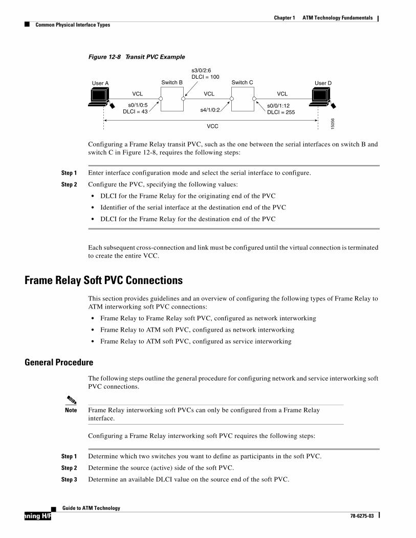
R
Chapter 1 ATM Technology FundamentalsCommon Physical Interface Types
Figure 12-8 Transit PVC Example
Configuring a Frame Relay transit PVC, such as the one between the serial interfaces on switch B and switch C in Figure 12-8, requires the following steps:
Step 1 Enter interface configuration mode and select the serial interface to configure.
Step 2 Configure the PVC, specifying the following values:
• DLCI for the Frame Relay for the originating end of the PVC
• Identifier of the serial interface at the destination end of the PVC
• DLCI for the Frame Relay for the destination end of the PVC
Each subsequent cross-connection and link must be configured until the virtual connection is terminated to create the entire VCC.
Frame Relay Soft PVC ConnectionsThis section provides guidelines and an overview of configuring the following types of Frame Relay to ATM interworking soft PVC connections:
• Frame Relay to Frame Relay soft PVC, configured as network interworking
• Frame Relay to ATM soft PVC, configured as network interworking
• Frame Relay to ATM soft PVC, configured as service interworking
General Procedure
The following steps outline the general procedure for configuring network and service interworking soft PVC connections.
Note Frame Relay interworking soft PVCs can only be configured from a Frame Relay interface.
Configuring a Frame Relay interworking soft PVC requires the following steps:
Step 1 Determine which two switches you want to define as participants in the soft PVC.
Step 2 Determine the source (active) side of the soft PVC.
Step 3 Determine an available DLCI value on the source end of the soft PVC.
User A
VCC
VCL
s0/1/0:5DLCI = 43
VCLVCL
s0/0/1:12DLCI = 255s4/1/0:2
s3/0/2:6DLCI = 100
Switch B Switch C User D
1505
6
unning H/F 4#Guide to ATM Technology
78-6275-03

Chapter 1 ATM Technology FundamentalsCommon Physical Interface Types
Step 4 Determine the destination (passive) side of the soft PVC.
Step 5 Determine the ATM address of the destination side of the soft PVC.
Step 6 If the destination side of the soft PVC is a Frame Relay interface, choose an available DLCI value. If the destination side of the soft PVC is an ATM interface, choose an available VPI/VCI value.
Step 7 Choose the interworking function type and the relevant interworking parameters (for example, de-bit/clp-bit mapping options).
Note If the soft PVC terminates on a Frame Relay interface, the soft PVC can only be configured as a network interworking connection. If the soft PVC terminates on an ATM interface, the soft PVC can be configured either as a network interworking connection or a service interworking connection.
Step 8 Configure the Frame Relay interworking soft PVC on the source side. See the following sections for configuration steps and examples.
Frame Relay to Frame Relay Network Interworking Soft PVCs
Figure 12-9 shows a Frame Relay to Frame Relay network interworking soft PVC between switch A and switch B.
Figure 12-9 Frame Relay to Frame Relay Network Interworking Soft PVC Example
Configuring a Frame Relay to Frame Relay network interworking soft PVC requires the following steps:
Step 1 Determine the source and destination interfaces.
Step 2 Determine an available DLCI value for the serial interface on the source side.
Step 3 Determine the ATM address for the destination serial interface.
Step 4 Determine an available DLCI value for the destination serial interface.
Step 5 Enter interface configuration mode and select the serial interface (source) to configure.
Step 6 Configure the soft PVC, specifying the following values:
• DLCI value for the serial interface on the source side
• ATM address of the destination serial interface
• DLCI value for the destination serial interface
User C
s0/1/0:5DLCI = 43
s0/0/1:9DLCI = 255
Switch A Switch B User D
1505
7
ATMnetwork
Frame Relayservice
Frame Relayservice
1-15Guide to ATM Technology
78-6275-03

R
Chapter 1 ATM Technology FundamentalsCommon Physical Interface Types
You can also specify the relevant interworking parameters, such as the Frame Relay to ATM traffic parameter mappings. You do not need to specify the interworking type; soft PVCs that originate and terminate on Frame Relay interfaces are configured as network interworking by default.
Frame Relay to ATM Service Interworking Soft PVCs
Figure 12-10 shows a Frame Relay to ATM service interworking soft PVC between switch A and switch B.
Figure 12-10 Frame Relay to ATM Service Interworking Soft PVC Example
Configuring Frame Relay to ATM service interworking soft PVC requires the following steps:
Step 1 Determine the source (serial) and destination (ATM) interfaces.
Step 2 Determine an available DLCI value for the serial interface.
Step 3 Determine the ATM address on the destination interface.
Step 4 Determine available VPI and VCI values on the ATM interface.
Step 5 Enter interface configuration mode and select the serial interface to configure.
Step 6 Configure the soft PVC, specifying the following values:
• DLCI value for the serial interface on the source side.
• ATM address of the destination interface.
• VPI and VCI values for the ATM interface.
• Interworking type, which is service in this case.
• Service interworking mode (transparent or translation). If the soft PVC terminates on an ATM interface, the default interworking type is service interworking in translation mode.
You can also specify the relevant interworking parameters, such as the Frame Relay to ATM traffic parameter mappings.
User C
s0/1/0:5DLCI = 43
a0/0/1VPI/VCI = 50/255
Switch A Switch B User D
1505
8
ATMnetwork
ATMFrame Relayservice
unning H/F 4#Guide to ATM Technology
78-6275-03

Chapter 1 ATM Technology FundamentalsCommon Physical Interface Types
Soft PVC Route Optimization
The soft PVC route optimization feature is supported on Frame Relay interfaces. For a detailed explanation of the feature, see the “Route Optimization for Soft PVCs” section on page 4-9.
Soft PVC route optimization must be enabled and configured to determine the point at which a better route is found and the old route is reconfigured. Enabling and configuring a Frame Relay interface with route optimization requires the following steps:
Step 1 From global configuration mode, enable route optimization and specify a threshold value.
Step 2 Enter interface configuration mode and select the serial interface to configure. You configure route optimization on the source end of a soft PVC only.
Step 3 Specify during what time of day and how often routes should be recomputed on this interface.
You can also manually trigger route optimization on a specific soft PVCC or PVPC.
Note Route optimization for soft permanent virtual connections should not be configured with constant bit rate (CBR) connections.
Existing Frame Relay to ATM Interworking Soft PVC Respecification
Existing Frame Relay to ATM interworking soft PVCs are torn down while an explicit path over the PVC is being respecified. However, you can configure a Frame Relay soft PVC to allow explicit paths to be respecified without tearing down connections. Existing connections are unaffected unless a reroute takes place, and then they use the newer explicit-path configuration.
For more information, see the “Soft PVCs with Explicit Paths” section on page 4-10.
Respecifying Frame Relay to ATM interworking soft PVCs requires configuring the soft PVC with the redo-explicit feature and related parameters, such as the explicit path precedence and partial path.
1-15Guide to ATM Technology
78-6275-03

R
Chapter 1 ATM Technology FundamentalsCommon Physical Interface Types
unning H/F 4#Guide to ATM Technology
78-6275-03
78-6275-03
I N D E X
A
AAL
in ATM reference model 1-12
service-dependent (table) 1-14
anycast signaling 2-4
ATM
addressing 1-12, 2-4
cell format 1-2, 1-4
description 1-1
device types 1-2
fundamentals 1-2
network interfaces 1-3, 3-2 to 3-6
physical interfaces 1-15 to 1-16
services 1-5
signaling 2-1
switch operation 1-9
virtual connection types 1-5
ATM adaptation layer. See AAL
ATM addresses
ATM switch router 2-6
autoconfigured scheme 2-7
automatic assignment for LANE components 6-11
components 2-4
formats
choosing 2-6
DCC 2-6
default 2-8
E.164 2-6, 2-11
figure 2-5
ICD 2-6
global uniqueness 7-15
ILMI 2-7, 2-9
ILMI address considerations 2-9
LANE 2-10
LANE templates 6-11
manually configured 2-10
obtaining 2-17
PNNI
autoconfigured 2-10
autoconfigured for single-level 7-13
hierarchical nature 7-15
planning 7-15
scalability 7-16
used by 2-7
registered 2-17
SVCs 1-12
See also E.164 addresses
ATM Address Resolution Protocol. See ATMARP
ATMARP
and ILMI 2-10
and RFC 1577 5-3
ATM network interfaces
autoconfiguration of 3-1
example 3-2
IISP 3-5
NNI 3-4
UNI 3-3
ATM reference model
ATM adaptation layer (AAL) 1-12
ATM layer 1-11
figure 1-11
OSI model 1-11
physical layer 1-11
service-dependent AAL 1-14
1Guide to ATM Technology

Index
ATM switch router
default address 2-6
inband management of
overview 5-8
PVCs with InATMARP 5-10
PVCs with static address mapping 5-10
SVCs with ATMARP 5-9
SVCs with static address mapping 5-10
LANE requirements 6-12
traffic management capabilities 10-1
autoconfiguration
ATM address
format 2-7
ATM addresses
PNNI, single-level 7-13
interface types 3-1
B
best-effort connection limits 10-11
broadcast-and-unknown server. See BUS
BUS
connection setup, example 6-9
function 6-4
multicast traffic, sending 6-8
C
CAC
algorithm 10-7
configurable parameters 10-8
description 10-5 to 10-6
parameter definitions 10-6
PNNI 7-7
resource management for tag switching 11-13
CAS 9-8
CDVT and MBS interface defaults 10-5
cell format
general 1-2
header 1-4
NNI format (figure) 1-5
UNI format (figure) 1-5
CES
advantages 9-10
applications 9-1
configuring
CDV 9-15
prerequisites 9-15
E1 port adapters 9-2 to 9-10
features 9-2
hard PVCs 9-18 to 9-19, 9-21 to 9-22
interworking function (CES-IWF) 9-3
limitations 9-10
on-hook detection 9-8
overview 9-1
soft PVCs 9-16 to 9-20, 9-22 to 9-27
structured services
bandwidth usage 9-20
channel-associated signaling 9-8
digital access and crossconnect system functionality 9-5
support 9-5
time slots 9-6
T1 port adapters 9-2 to 9-10
unstructured services
bandwidth usage 9-17
support 9-4
CES-IWF 9-3
channel-associated signaling. See CAS
channelized DS3 port adapter
configuration
channel groups 12-5
guidelines 12-4
overview 12-4
2Guide to ATM Technology
78-6275-03

Index
physical interface 12-4
T1 lines 12-4
description 12-3
channelized E1 port adapter
configuration
channel groups 12-7
guidelines 12-6
overview 12-6
physical interface 12-7
description 12-5
time slot mapping 12-5
circuit emulation services. See CES
classical IP over ATM
description 5-2
example (figure) 5-3
RFC 1577, defined in 5-3
clocking. See network clocking
closed user groups. See CUGs
complex node representation
aggregation modes compared 7-38
exception thresholds 7-37
implementation guidelines 7-38
routing accuracy of 7-36
simple node representation, compared 7-35
terminology 7-36
Connection Admission Control. See CAC
connection traffic table. See CTT
controlled link sharing 10-9
conventions xvii
CoS
CTT rows 11-12
resource management CAC not supported 11-13
service class to weight mapping
hierarchical VP tunnels 11-10
physical ports 11-10
threshold group for TBR classes 11-11
crankback mechanism 7-8
CTT
Frame Relay to ATM interworking 12-10
row allocations and defaults 10-3
rows for tag switching virtual connections 11-12
traffic and service contract 10-3
CUGs
configuration overview 2-21
example (figure) 2-20
interlock codes for 2-19
overview 2-18
D
data rate for physical interfaces 1-15
documentation
CD-ROM xviii
online xvii
printed xvii
document conventions xvii
DS0 channels. See DS0 time slots
DS0 time slots
Frame Relay to ATM interworking
channel groups, forming 12-5
DS3 interfaces 12-3
E1 interfaces 12-5
mapping example (figure) 12-3
structured CES
example (figure) 9-6
mapping 9-6
E
E.164 addresses
autoconversion
AESA example (figure) 2-16
comparison (table) 2-14
description 2-13
ZDSP example (figure) 2-15
3Guide to ATM Technology
78-6275-03

Index
conversion options 2-12
encoding for PNNI 7-13
gateway translation
description 2-12
example (figure) 2-12
NSAP encoded format 2-6
one-to-one translation 2-16
signaling of 2-11
types 2-11
E1 port adapters
CES
description 9-2
structured services 9-5
time slots, example 9-7
unstructured services 9-4
time slots
CES 9-6
Frame Relay to ATM interworking 12-5
See also DS0 time slots
ELANs
address resolution in 6-7
joining 6-7
virtual LANs, compared 6-5
See also LANE
emulated LANs. See ELANs
exception thresholds 7-37
explicit paths for soft PVCs
description 4-10
PNNI 7-29
F
FIB 11-3
Forwarding Information Base. See FIB
Frame Relay to ATM interworking
channelized DS3 port adapter 12-3 to 12-5
channelized E1 port adapter 12-5 to 12-7
configuring
encapsulation 12-8
overview 12-7
serial interface type 12-8
LMI 12-8 to 12-9
network interworking 12-2
overview 12-1
resource management
configuration overview 12-9
CTT description 12-10
interface configuration overview 12-11
service interworking 12-2
virtual connections 12-11 to 12-19
framing overhead 10-14
framing type for physical interfaces 1-15
funnel signaling
description 2-21
example (figure) 2-21
G
GCAC
and PTSP exchanges 7-5
description 7-7
in call routing, example 7-8
Generic Call Admission Control algorithm. See GCAC
H
hard PVCs
structured services 9-21
unstructured services 9-18
hardware-dependent features 10-16
Hello protocol 7-5
4Guide to ATM Technology
78-6275-03

Index
hierarchical VP tunnels
description 4-16
restrictions 4-17
service category support 10-11
service class to TBR class mapping 11-10
I
IISP
description 3-5
example (figure) 3-5
interface configuration 3-6
routing
advantages 7-3
description 7-1
limitations 7-3
ILMI
ATM addresses 2-9
ATM address migration 2-9
autoconfiguration with 3-1
InATMARP 5-4
individual traffic parameter maximums 10-11
Integrated Local Management Interface. See ILMI
interface category support 10-11
interface output pacing 10-21
interface overbooking 10-12
interface queue thresholds per service category 10-17
Interim Interswitch Signaling Protocol. See IISP
Inverse ATM address resolution protocol. See InATMARP
L
LANE
address assignment for components 6-11
addressing requirements 6-10
address resolution 6-7
advantages 6-12
applications 6-2
assigning components 6-12
ATM addresses 2-10
broadcast-and-unknown server (BUS) 6-4 to 6-9
client (LEC) 6-4 to 6-9
components 6-4
configuration server (LECS) 6-5 to 6-11
configuring
overview 6-13
worksheet 6-15
description 6-1
example 6-8
fault tolerance 6-17
function of network devices in 6-3
implementation considerations 6-10
limitations 6-12
multicast traffic 6-8
operation 6-3
protocol stack 6-3
router and switch requirements 6-12
server (LES) 6-4 to 6-7
SSRP 6-17
VCC types 6-5
LANE configuration server. See LECS
LAN emulation. See LANE
LAN emulation client. See LEC
LAN emulation configuration server. See LECS
LAN emulation server. See LES
Layer 3 protocols over ATM 5-1 to 5-5
LEC
address resolution 6-8
connection setup, example 6-9
function 6-4
joining an emulated LAN 6-7
VCCs for 6-6
LECS
address database 6-11
function 6-5
joining an emulated LAN 6-7
5Guide to ATM Technology
78-6275-03
Index
LES
function 6-4
joining an emulated LAN 6-7
VCCs for 6-6
LGNs
complex node representation 7-35
configuring 7-23
description 7-10
LMI configuration
keepalive interval 12-9
LMI type 12-8
overview 12-8
polling and timer interval 12-9
Local Management Interface. See LMI
logical group nodes. See LGNs
M
map lists. See static map lists
MaxCR
in framing overhead 10-14
in interface overbooking 10-12
maximum cell rate. See MaxCR
maximum queue size per interface 10-17
MPOA
advantages 6-21
configuration overview 6-21
description 6-19
limitations 6-21
operation 6-20
multiprotocol encapsulation over ATM
description 5-2
RFC 1483, defined in 5-4
Multiprotocol Label Switching (MPLS). See tag switching
Multiprotocol over ATM. See MPOA
N
NCDP
consideration when using 8-8
description 8-6
operation, example 8-6
network clocking
CBR and VBR-RT traffic 8-1
CES 8-2
clock distribution modes 8-3
clocking modes for CES
adaptive 9-14
characteristics 9-11
description 9-11
SRTS 9-12
synchronous 9-12
clock sources
network clock module 8-5
quality 8-2
revertive behavior 8-4
configuring
manual 8-11
NCDP 8-10
definition 8-1
example 8-3
NCDP 8-6 to 8-8
overview 8-1
Network Clocking Distribution Protocol. See NCDP
network clock module
BITS derived clocking 8-6
oscillator quality 8-6
resilience 8-5
Network-Network Interface. See NNI
NNI
cell header format 1-5
configuring 3-5
example 3-4
example (figure) 3-4
6Guide to ATM Technology
78-6275-03

Index
nondefault PVCs
configuring 4-11
uses 4-11
well-known values 4-11
O
outbound link distance 10-10
oversubscription factor 10-16
P
peer group leaders. See PGLs
permanent virtual connections. See PVCs
permanent virtual paths. See PVPs
PGLs 7-10
physical interfaces
common (table) 1-16
description 1-15 to 1-16
media types 1-15
PNNI
aggressive aggregation mode 7-34, 7-38
ATM addresses 2-10, 7-13 to 7-17
best link aggregation mode 7-34, 7-38
CAC 7-7
call routing 7-8
complex node representation 7-35 to 7-39
crankback mechanism 7-8
database synchronization 7-5
E.164 addresses
encoding 7-13
justification 7-13
GCAC 7-7
Hello protocol 7-5
hierarchical
implementation considerations 7-12
hierarchical topology 7-9 to 7-12
higher levels
implementation considerations 7-22
LGNs 7-23
node election leadership priority 7-24
node names 7-24
overview 7-21
parent node designation 7-24
PGLs 7-23
summary addresses 7-25
LGNs 7-10, 7-23, 7-35
lowest level
ATM address 7-18
node level 7-18
overview 7-18
scope mapping 7-20
static routes 7-19
summary addresses 7-19
metrics and attributes 7-6
operation 7-8
overview 7-4
peer groups 7-10
PGLs 7-10
protocol parameters
Hello exchanges 7-39
resource management poll interval 7-40
PTSP exchanges 7-5, 7-39
reachability information 7-6
route selection tuning
background route computation 7-26
links, parallel, and alternate 7-27
manually configured explicit paths 7-29
maximum administrative weight percentage 7-28
precedence of reachable addresses 7-28
routing features 7-4
signaling features 7-4
single-level
autoconfigured addresses 7-13
configuration 7-18
when suitable 7-9
7Guide to ATM Technology
78-6275-03

Index
topology attributes
administrative weight 7-30
aggregation mode 7-33
aggregation tokens 7-32
route redistribution 7-32
significant change thresholds 7-34
transit call restriction 7-32
point-to-multipoint connections
ATM solutions 1-7
description 1-6
signaling 2-4, 2-21
port adapters
CES 9-2
Frame Relay to ATM interworking 12-1
Private Network-Network Interface. See PNNI
PTSP exchanges
description 7-5
tuning 7-39
PVCs
applications 4-4
configuration overview 4-5
connecting to VP tunnels 4-18
Frame Relay to ATM interworking
network interworking 12-13
service interworking 12-14
terminating service interworking 12-14
transit 12-15
nondefault well-known 4-11
point-to-multipoint 4-6
terminating 4-5
with InATMARP 5-6, 5-10
with static address mapping 5-7, 5-10
See also hard PVCs
See also soft PVCs
PVPs
network example 4-7
point-to-multipoint 4-7
Q
QoS
default objective table 10-4
parameters 1-13
parameters per service category (table) 10-2
PNNI 7-5
quality of service. See QoS
R
resource management. See traffic management
RFC 1483 5-4
RFC 1577
ATMARP mechanism 5-3
InATMARP mechanism 5-4
provisions 5-3
route optimization for soft PVCs 4-9
routing
IISP 7-1 to 7-3
PNNI 7-4 to 7-9
S
scheduler and service class 10-22
service categories
characteristics 1-14
description 1-13
table 1-13
service category limit 10-17
service category parameters 10-2
SGCP
advantages 9-29
description 9-27
operation 9-29
shaped VP tunnels
description 4-15
restrictions 4-16
8Guide to ATM Technology
78-6275-03

Index
signaling
about 2-1
ABR connections 2-4
anycast 2-4
connection setup 2-2
E.164 addresses 2-11
features 2-18
NNI 2-3
point-to-multipoint connections 2-4
point-to-multipoint funnel 2-21
proxy 2-4
QoS parameters 2-4
UNI 2-3
virtual UNI 2-4
signaling VPCI 4-18
Simple Gateway Control Protocol. See SGCP
Simple Server Redundancy Protocol. See SSRP
soft PVCs
advantages 2-2, 4-4
CES
configuration guidelines 9-16
structured services 9-22, 9-24, 9-26
unstructured services 9-19
example 4-8
explicit paths 4-10, 7-29
Frame Relay to ATM interworking
configuration overview 12-16
network interworking 12-17
respecifying 12-19
route optimization 12-19
service interworking 12-18
route optimization 4-9
soft PVPs
advantages 2-2, 4-4
example 4-9
SSRP
configuration overview 6-18
considerations 6-18
description 6-17
operation 6-17
static map lists
description 5-5
PVCs 5-7
SVCs 5-7
sustained cell rate margin factor 10-9
SVCs
applications 4-4
ATMARP 5-6, 5-9
static address mapping 5-7, 5-10
VPI/VCI ranges 4-11
switched virtual connections. See SVCs
T
T1 port adapters
description 9-2
structured services 9-5
time slots, example 9-7
unstructured services 9-4
Tag Distribution Protocol. See TDP
Tag Forwarding Information Base. See TFIB
Tag Information Base. See TIB
9Guide to ATM Technology
78-6275-03

Index
tag switching (MPLS)
advantages 11-4
components 11-2
configuring
interfaces 11-6
loopback interface 11-6
overview 11-5
routing protocol 11-6
TDP control channel 11-7
VPI range 11-7
VP tunnels 11-7
CoS 11-9 to 11-13
FIB 11-3
hardware and software restrictions 11-5
hierarchical VP tunnels 11-10
limitations 11-5
network example (figure) 11-2
operation 11-3
overview 11-1
tag edge routers in 11-2
tag switches in 11-2
TDP 11-2, 11-7
TFIB 11-3
TIB 11-3
VC merge 11-8
TDP
control channels 11-7
used by tag edge routers 11-2
TFIB 11-3
threshold groups 10-18
TIB 11-3
time slots. See DS0 time slots
traffic management
best-effort connection limits 10-11
CAC
description 10-5 to 10-6
tag switching not supported 11-13
capabilities 10-1
cell queuing 10-16
interface queue thresholds per service category 10-17
maximum queue size per interface 10-17
oversubscription factor 10-16
service category limit 10-17
threshold groups 10-18
congestion notification 10-20
controlled link sharing 10-9
Frame Relay to ATM interworking 12-9
framing overhead 10-14
hardware resource mechanisms 10-14
individual traffic parameter maximums 10-11
interface category support 10-11
interface overbooking 10-12
outbound link distance 10-10
output scheduling
interface output pacing 10-21
scheduler and service class 10-22
sustained cell rate margin factor 10-9
threshold groups
defaults 10-18
operation 10-19
traffic and service contract
CDVT and MBS interface defaults 10-5
configurable parameters 10-3
connection setup 1-13
CTT 10-3
default QoS objective table 10-4
service category parameters 10-2
traffic policing 10-15
traffic shaping 10-21
UPC
default behavior 10-15
default CDVT and MBS 10-16
purpose 10-15
traffic parameters 1-13
traffic policing 10-15
traffic shaping 10-21
10Guide to ATM Technology
78-6275-03

Index
U
UNI
autoconfiguration with ILMI 2-7, 3-1
cell header format 1-4
configuration 3-3
example (figure) 3-3
signaling 2-3
specifications 2-3
virtual 4-18
UPC 10-15
Usage Parameter Control. See UPC
User-Network Interface. See UNI
V
virtual channel identifier. See VPI/VCI
virtual connections
applications 4-4
autoconfigured parameters 4-3
components 4-2
Frame Relay to ATM interworking
characteristics 12-12
configuration overview 12-11
configuration prerequisites 12-12
PVCs 12-13 to 12-16
soft PVCs 12-16 to 12-19
point-to-multipoint 1-6
supported types (table) 4-3
transit and terminating 4-2
types 1-5, 4-2
See also PVCs
See also PVPs
virtual path. See VP switching and VP tunnels
virtual path identifier. See VPI/VCI
virtual UNI
signaling 2-4
signaling VPCI 4-18
voice over ATM
with CES 9-1
with SGCP 9-27
VPI/VCI
purpose 1-6
ranges for SVPs and SVCs
description 4-11
maximum (table) 4-12
VP switching
description 1-9
figure 1-9
VP tunnels
between source and destination switches (figure) 11-8
CES through 9-22
example (figure) 4-14
general description 4-13
PVC connection to 4-18
signaling VPCI 4-18
single service category 4-14
tag switching on 11-7
types 4-14
See also hierarchical VP tunnels
See also shaped VP tunnels
W
well-known PVCs
nondefault 4-11
well-known virtual channels (table) 4-11
11Guide to ATM Technology
78-6275-03

Index
12Guide to ATM Technology
78-6275-03