© University of Reading 2007 www.reading.ac.uk

Symposium on Air Pollution

22 July 2009

Chemical Transformation During Intercontinental TransportJohn Methven and Michelle Cain,

Department of Meteorology, University of Reading

2

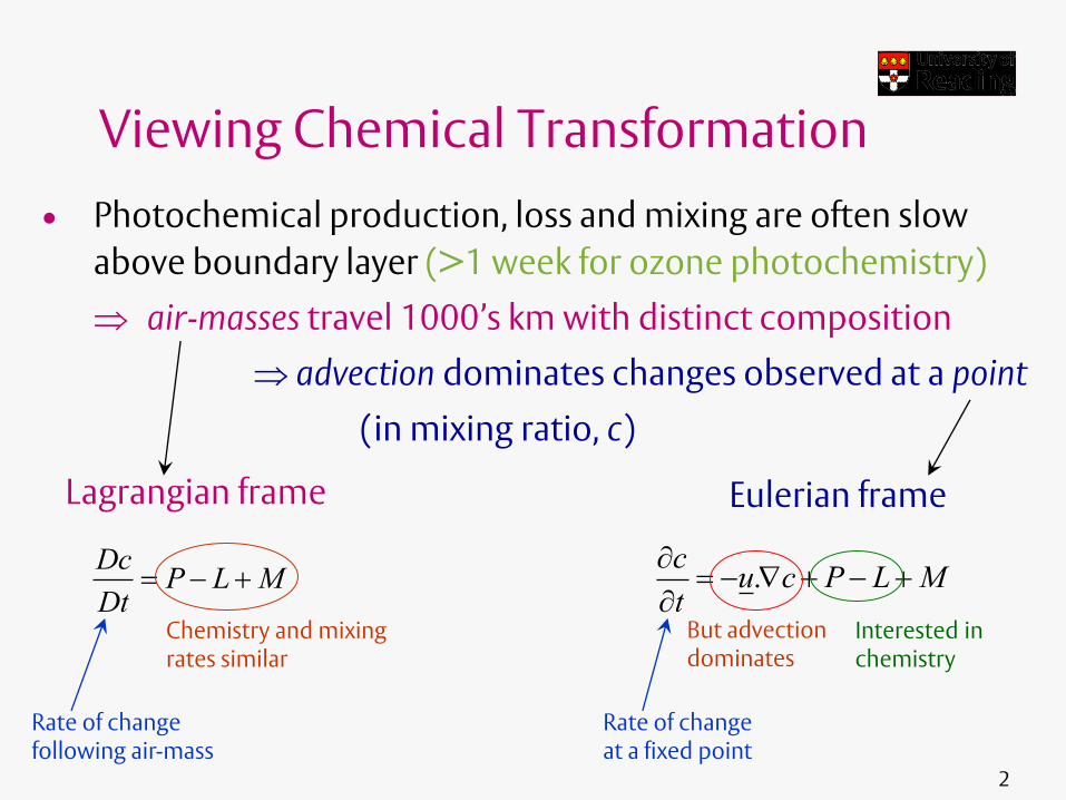
Viewing Chemical Transformation

• Photochemical production, loss and mixing are often slow

above boundary layer (>1 week for ozone photochemistry)

air-masses travel 1000’s km with distinct composition

advection dominates changes observed at a point

(in mixing ratio, c)

DcP L M

Dt .

cu c P L M

t

Lagrangian frame Eulerian frame

Rate of change following air-mass

Rate of change at a fixed point

But advection dominates

Interested in chemistry

Chemistry and mixing rates similar

3

Using Lagrangian framework

Can be used in 3 ways:

1. Formulation of a chemical transport model

2. Diagnosis of model results

3. Design of observation strategy Used here but not essential for 2 and 3

The rationale for a “quasi-Lagrangian experiment” where the same air-mass is sampled several times over the course of a week.

Quasi- means air parcel is not tagged (e.g., by balloon) but location is estimated using trajectory calculation.

4

A “Quasi-Lagrangian Experiment”

Reduce uncertainty at airReduce uncertainty at air--mass origins by observing there.mass origins by observing there.

Chemistry is slow, so need to track air masses for many days (1000s of km).

Sample polluted air masses leaving the continental BL.

Follow across Atlantic since no emissions after USA.

Scale of problem requires several coordinated research aircraft.

ITCT-Lagrangian 2K4 Experiment took place within the framework of the ICARTT campaign in summer 2004:

International Consortium for Atmospheric Research on Transport and Transformation.

5

ICARTT Campaign – Aircraft flight tracks

FAAM BAe146, based in Faial, Azores.

Slide: M. Evans, University of Leeds

6

e.g., New York to Spain – 4 flights linked by trajectories

12

3

Trajectories from BAe146 flight track (blue) back and forwards for 3.5 days.

Best matches with trajectories from other flight tracks.

2 31

4

4

+3

to Azores

7

Did the aircraft sample the sameair mass many times?

Two independent matching methods:

1. Trajectory models driven by met. analyses2. Hydrocarbon fingerprints (bottled air samples)

Search for coincidentcoincident matches:two samples with matching HC fingerprint are also linked by matching trajectories.

Quality of matches assessed using independent observations of long-lived tracers

8

5 Lagrangian cases verified

15 July - New York to Spain to Azores: NOAA/NASA FAAM DLR FAAM

18 July - Alaskan Fire Plume NASA FAAM DLR

20 July - New York to Ireland (low level) NOAA(x3)/NASA DLR(x2)

25 July - Upper level frontal export NASA(x2) FAAM DLR

25 July - Low level frontal export NOAA(x2) FAAM(x2)

9

Modelling the Lagrangian cases

Trajectories calculated forwards from upwind flight tracks.

• Released every 10s from Lagrangian match time window

ensemble of trajectories representing initial condition uncertainty

Cambridge Tropospheric Trajectory model of Chemistry and Transport

(CiTTyCAT) initialised using all available concentration data upwind

• Photochemistry scheme with 90 species (intermediate)

• Mixing between ensemble members by assuming:

– Vertical gradients dominate

– Averaging members to create evolving vertical profile

– Constant flux boundary layer and eddy diffusion above

• Emissions and dry deposition by imposing flux boundary condition

• Wet deposition proportional to precipitation rate from ECMWF model

10

NY-Spain-Azores ensemble simulationO

zon

e →

Nit

ric

acid

→C

O →

NO

→

Time →

USA day 0

Azores day 4

Spainday 7

Azores day 10

Long-lived

Short-lived

(absent at night)

Less reactive but sensitive to deposition

11

Quantitative model evaluation

[OH] indirectly from hydrocarbon obs

12

Integrated effect of chemistry and physics∆

(Ozo

ne

) →

∆(N

itri

c ac

id) →

∆(C

O) →

∆(N

O) →

Time →

Net chemistry

Deposition and mixing

Fast chemistryDeposition and mixing

Loss by reaction with OH

13

Sensitivity to model parameters7 ensembles for NY-Ireland case

Red triangles

= obs. mean and s-deviation

Black diamonds

= control expt. ensemble mean and s-deviation

Wet deposition too weak?

Not mixing with clean enough air?

Dry deposition stronger?

14

Integrated effect of chemistry and physics

Bold lines

= chemistry

Dotted lines

= deposition/mixing

15

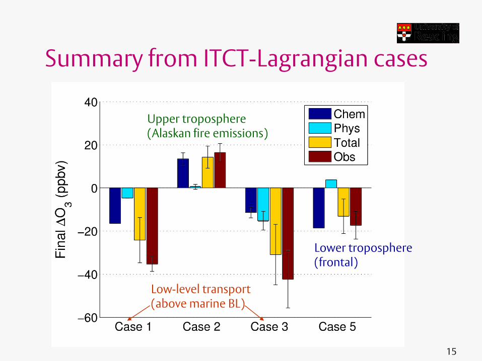
Summary from ITCT-Lagrangian cases

Low-level transport (above marine BL)

Upper troposphere (Alaskan fire emissions)

Lower troposphere (frontal)

16

Conclusions

• Photochemical model of intermediate complexity simulates chemical

changes consistent with those from observations.

• Would not have been possible to deduce this without Lagrangian expt!

• In upper trop. and frontal cases, photochemistry dominates mixing.

• Net ozone increase in long-range only occurs in upper troposphere.

• In long-range regime, process uncertainty from greatest to least effect:

mixing → deposition (wet & dry) → clouds → photochemistry