Chee Han Tan Last modi ed : January 13, 2018

Math 6410 : Ordinary Differential Equations

Chee Han Tan

Last modified : January 13, 2018

Contents

Preface 5

1 Initial Value Problems 7

1.1 Introduction . . . . . . . . . . . . . . . . . . . . . . . . . . . . . . . . . . . . . . 7

1.2 Planar Dynamics . . . . . . . . . . . . . . . . . . . . . . . . . . . . . . . . . . . 9

1.3 Existence and Uniqueness . . . . . . . . . . . . . . . . . . . . . . . . . . . . . . 9

1.3.1 Picard’s Method of Successive Approximation . . . . . . . . . . . . . . . 10

1.3.2 Dependence on Initial Conditions . . . . . . . . . . . . . . . . . . . . . . 13

1.4 Manifolds . . . . . . . . . . . . . . . . . . . . . . . . . . . . . . . . . . . . . . . 15

1.5 Limit Cycle and Poincare-Bendixson Theorem . . . . . . . . . . . . . . . . . . . 15

1.5.1 Orbits, Invariant Sets and ω-Limit Sets . . . . . . . . . . . . . . . . . . . 16

1.5.2 Local Transversals . . . . . . . . . . . . . . . . . . . . . . . . . . . . . . 18

1.5.3 Poincare-Bendixson Theorem . . . . . . . . . . . . . . . . . . . . . . . . 18

1.6 Problems . . . . . . . . . . . . . . . . . . . . . . . . . . . . . . . . . . . . . . . . 21

2 Linear Systems and Stability of Nonlinear Systems 27

2.1 Autonomous Linear Systems . . . . . . . . . . . . . . . . . . . . . . . . . . . . . 27

2.1.1 Matrix Exponential . . . . . . . . . . . . . . . . . . . . . . . . . . . . . . 27

2.1.2 Normal Forms . . . . . . . . . . . . . . . . . . . . . . . . . . . . . . . . . 28

2.2 Non-Autonomous Linear Systems . . . . . . . . . . . . . . . . . . . . . . . . . . 31

2.2.1 Homogeneous Equation . . . . . . . . . . . . . . . . . . . . . . . . . . . . 31

2.2.2 Inhomogeneous equation. . . . . . . . . . . . . . . . . . . . . . . . . . . . 33

2.2.3 Stability and Bounded Sets . . . . . . . . . . . . . . . . . . . . . . . . . 35

2.2.4 Equations With Coefficients That Have A Limit . . . . . . . . . . . . . . 37

2.3 Floquet Theory . . . . . . . . . . . . . . . . . . . . . . . . . . . . . . . . . . . . 39

2.3.1 Floquet Multipliers . . . . . . . . . . . . . . . . . . . . . . . . . . . . . . 39

2.3.2 Stability of Limit Cycles . . . . . . . . . . . . . . . . . . . . . . . . . . . 42

2.3.3 Mathieu Equation . . . . . . . . . . . . . . . . . . . . . . . . . . . . . . . 45

2.3.4 Transition Curves . . . . . . . . . . . . . . . . . . . . . . . . . . . . . . . 47

2.3.5 Perturbation Analysis of Transition Curves . . . . . . . . . . . . . . . . . 48

2.4 Stability of Periodic Solutions . . . . . . . . . . . . . . . . . . . . . . . . . . . . 51

2.5 Stable Manifold Theorem . . . . . . . . . . . . . . . . . . . . . . . . . . . . . . . 53

2.6 Centre Manifolds . . . . . . . . . . . . . . . . . . . . . . . . . . . . . . . . . . . 57

2.7 Problems . . . . . . . . . . . . . . . . . . . . . . . . . . . . . . . . . . . . . . . . 60

3

4 Contents

3 Perturbation Theory 633.1 Basics of Perturbation Theory . . . . . . . . . . . . . . . . . . . . . . . . . . . . 63

3.1.1 Asymptotic Expansion . . . . . . . . . . . . . . . . . . . . . . . . . . . . 633.1.2 Naive Expansions . . . . . . . . . . . . . . . . . . . . . . . . . . . . . . . 65

3.2 Method of Multiple Scales . . . . . . . . . . . . . . . . . . . . . . . . . . . . . . 663.3 Averaging Theorem: Periodic Case . . . . . . . . . . . . . . . . . . . . . . . . . 683.4 Phase Oscillators and Isochrones . . . . . . . . . . . . . . . . . . . . . . . . . . 683.5 Problems . . . . . . . . . . . . . . . . . . . . . . . . . . . . . . . . . . . . . . . . 69

4 Boundary Value Problems 714.1 Compact Symmetric Linear Operators . . . . . . . . . . . . . . . . . . . . . . . 714.2 Linear Differential Operators . . . . . . . . . . . . . . . . . . . . . . . . . . . . . 76

4.2.1 Formal Adjoint . . . . . . . . . . . . . . . . . . . . . . . . . . . . . . . . 774.2.2 A Simple Eigenvalue Problem . . . . . . . . . . . . . . . . . . . . . . . . 784.2.3 Adjoint Boundary Conditions . . . . . . . . . . . . . . . . . . . . . . . . 794.2.4 Self-Adjoint Boundary Conditions . . . . . . . . . . . . . . . . . . . . . . 80

4.3 Eigenvalue Problems and Spectral Theory . . . . . . . . . . . . . . . . . . . . . 814.3.1 Discrete Spectrum . . . . . . . . . . . . . . . . . . . . . . . . . . . . . . 824.3.2 Continuous Spectrum . . . . . . . . . . . . . . . . . . . . . . . . . . . . . 824.3.3 Mixed Spectrum . . . . . . . . . . . . . . . . . . . . . . . . . . . . . . . 834.3.4 Rayleigh-Ritz Variational Principle . . . . . . . . . . . . . . . . . . . . . 84

4.4 Distribution . . . . . . . . . . . . . . . . . . . . . . . . . . . . . . . . . . . . . . 894.4.1 Distributions and Test Functions . . . . . . . . . . . . . . . . . . . . . . 904.4.2 Weak Derivatives . . . . . . . . . . . . . . . . . . . . . . . . . . . . . . . 91

4.5 Green’s Function . . . . . . . . . . . . . . . . . . . . . . . . . . . . . . . . . . . 934.5.1 Fredholm Alternative . . . . . . . . . . . . . . . . . . . . . . . . . . . . . 934.5.2 Green’s Functions for Homogeneous Boundary Conditions . . . . . . . . 944.5.3 Modified Green’s Function . . . . . . . . . . . . . . . . . . . . . . . . . . 974.5.4 Eigenfunction Expansions . . . . . . . . . . . . . . . . . . . . . . . . . . 984.5.5 Inhomogeneous Boundary Conditions . . . . . . . . . . . . . . . . . . . . 99

4.6 Problems . . . . . . . . . . . . . . . . . . . . . . . . . . . . . . . . . . . . . . . . 101

Preface

These notes are largely based on Math 6410: Ordinary Differential Equations course, taughtby Paul Bressloff in Fall 2015, at the University of Utah. Additional examples or remarksor results from other sources are added as we see fit, mainly to facilitate our understanding.These notes are by no means accurate or applicable, and any mistakes here are of courseour own. Please report any typographical errors or mathematical fallacy to me by [email protected].

5

mailto:[email protected]

Chapter 1

Initial Value Problems

1.1 Introduction

We begin by studying the initial value problem (IVP)x = f(x), x ∈ U, f : U −→ Rn

x(0) = x0 ∈ U, x = (x1, . . . , xn)T(IVP)

where U is an open subset of Rn. Unless stated otherwise, f will be as smooth as we needthem to be. First order ODEs are of fundamental importance, due to the fact that any nthorder ODE can be written as a system of n first order ODEs.

Example 1.1.1 (Newtonian Dynamics). Consider mx = −γx + F (x), where −γx is thedamping term and F (x) some external force. This can be written as a system of first orderODEs:

x = y = f1(x, y),

y = − γmy +

F (x)

m= f2(x, y).

• Observe that we have a conservative system if γ = 0. Indeed, let V (x) = −∫ x

F (s) dsbe the potential function. Multiplying the ODE by x yields

mxx = −(dV

dx

)x =⇒ d

dt

(1

2mx2

)= − d

dtV (x(t)).

Thus, we obtain the well-known conservation of energy:1

2mx2 + V (x) = E.

• Let p = mx be the momentum, and define the Hamiltonian as

H = H(x, p) =1

2mp2 + V (x).

We have the following Hamilton’s equations:

x =∂H

∂p, p = −∂H

∂x.

7

8 1.1. Introduction

An important property of Hamiltonian is they are conserved over time, i.e.

dH

dt=∂H

∂xx+

∂H

∂pp = 0.

Example 1.1.2 (Classical Predator-Prey Model). Let N(t) be the amount of bacteria, andassume that N is large enough so that we can treat it as a continuous variable. One simplemodel is the following:

N = NK

(1− N

Nmax

)− d, N(0) = N0.

Non-dimensionalising the system with the dimensionless parameters

x =N

Nmax

, τ = Kt, D =d

KNmax

yields the dimensionless equation x = (1 − x)x − D. This is a bifurcation problem, with bi-furcation paramter D. If 0 < D < 1/4, then there eixsts 2 fixed points; otherwise there is nofixed points.

From a geometric perspective, it seems rather natural to think of solution to (IVP) as afunction of initial value x(0) = x0 and time t. This motivates the definition of a flow.

Definition 1.1.3. Let U ⊂ Rn and f ∈ C1(U). Given x0 ∈ U , let φt(x0) = φ(x0, t) be thesolution of (IVP) with t ∈ I(x0), where I(x0) is the maximal time interval over which a uniquesolution exists. Such set of mappings φt is called the flow of the vector field f .

• For a fixed x0 ∈ U , φ(x0, ·) : I(x0) −→ U defines a curve or trajectory, Γ(x0) of thesystem through x0. Specifically,

Γ(x0) =x ∈ U : x = φt(x0), t ∈ I(x0)

.

• If x0 varies over a set M ⊂ U , then the flow φt : M −→ U defines the motion of a cloudof points in M .

Theorem 1.1.4 (Time-shift invariance). For any x0 ∈ U , if t ∈ I(x0) and s ∈ I(φt(x0)),s > 0, then s+ t ∈ I(x0) and φs+t(x0) can be expressed as φs+t(x0) = φs(φt(x0)).

Proof. Let I(x0) = (α, β) be the maximal time interval over which there exists a uniquesolution. Consider the function x : (α, s+ t) −→ U defined by

x(r) =

φ(r, x0) if r ∈ (α, t],

φ(r − t, φt(x0)) if r ∈ [t, s+ t].

We see that x(r) is a solution of the IVP on (α, s+ t). Hence, s+ t ∈ I(x0) and uniqueness ofsolution gives

φs+t(x0) = x(s+ t) = φ(s, φt(x0)) = φs(φt(x0)).

Initial Value Problems 9

Remark 1.1.5. The result is trivial if s = 0. The result holds for s < 0 by evolving backwardsin time. A corollary of the above theorem is that φ−t(φt(x0)) = φt(φ−t(x0)) = x0, i.e. we havean abelian group structure here!

Remark 1.1.6. There exists ODEs in which solution does not exist globally, even if f ∈ C1(U).

Consider the ODE x = f(x) =1

x, where f ∈ C1(U) with U = x ∈ R : x > 0. For an

initial condition x(0) = x0 ∈ U , a solution to this IVP is given by φt(x0) =√

2t+ x20, with

I(x0) =

(−x2

0

2,∞)

.

1.2 Planar Dynamics

Consider the general autonomous second order systemx = X(x, y)

y = Y (x, y)

Assuming existence and uniqueness, then paths only cross at fixed points.

1.3 Existence and Uniqueness

In this section, we focus on establishing sufficient conditions such that there exists a uniquesolution to (IVP). Not suprisingly, regularity of f : U −→ Rn plays an important role, as weshall see below.

(a) Continuity of f is not sufficient to guarantee uniqueness of a solution.

• Consider x = 3x2/3, x(0) = 0. One solution is the trivial solution x(t) ≡ 0 for allt ≥ 0. Another solution is obtained by using separation of variable:

1

3

∫ x

0

1

s2/3ds = t =⇒ x(t) = t3.

• Observe that f is continuous but not differentiable at the origin.

(b) A solution can become unbounded at some finite time t = T , i.e. finite-time blow up.

• Consider x = x2, x(0) = 1. We have two branches of solution, x(t) =1

1− t, depending

on the initial condition.

• In this case, our solution is only defined on t ∈ (−∞, 1), and limt→1−

x(t) =∞.

• The other branch is defined on t ∈ (1,∞), but is not reached by the given initialcondition.

Definition 1.3.1.

10 1.3. Existence and Uniqueness

(a) We say that f : Rn −→ Rn is differentiable at x0 ∈ Rn if there exists a linear transfor-mation Df(x0) ∈ L(Rn), called the n× n Jacobian matrix such that

lim|h|→0

|f(x0 + h)− f(x0)−Df(x0)h||h|

= 0.

(b) Let U be an open subset of Rn. A function f : U −→ Rn is said to satisfy a Lipschitzcondition on U if there exists K > 0 such

|f(x)− f(y)| ≤ K|x− y| for all x, y ∈ U.

(c) A function f : U −→ Rn is said to be locally Lipschitz on U if for every x0 ∈ U , thereexists an ε-neighbourhood Nε(x0) ⊂ U and K0 > 0 such that

|f(x)− f(y)| ≤ K0|x− y| for all x, y ∈ Nε(x0).

Theorem 1.3.2. C1(U) =⇒ locally Lipschitz on U .

Proof. Choose an arbitrary x0 ∈ U and suppose x, y ∈ Bε(x0) ⊂ U , with K = maxx∈Bε(x0)

‖Df(x)‖.

Convexity of Bε(x0) means that x + su ∈ Bε(x0) for 0 ≤ s ≤ 1, with u = y − x. LetF (s) = f(x+ su), then F ′(s) = Df(x+ su) · u and

|f(y)− f(x)| = |F (1)− F (0)| =∣∣∣∣∫ 1

0

F ′(s) ds

∣∣∣∣ ≤ ∫ 1

0

|Df(x+ su) · u| ds

≤ K

∫ 1

0

|x− y| ds = K|x− y|.

1.3.1 Picard’s Method of Successive Approximation

Let x(t) be a solution to (IVP), that is x(t) is a continuous function satisfying the integralequation

x(t) = x0 +

∫ t

0

f(x(s)) ds,

and vice-versa. Successive approximations to the solution of the integral equation are definedby the sequence of functions

u0(t) = x0, uk+1(t) = x0 +

∫ t

0

f(uk(s)) ds. (1.3.1)

Example 1.3.3. Consider x = Ax with x(0) = x0.

u1(t) = x0 +

∫ t

0

Ax0 ds = x0(1 + At).


u2(t) = x0 +

∫ t

0

A[x0(1 + As)] ds = x0

(1 + At+

A2t2

2

).

......

...

uk(t) = x0

(1 + At+ . . .+

(At)k

k!

)−→ x0e

At as k −→∞.

Theorem 1.3.4 (Fundamental Theorem of Existence and Uniqueness of ODEs).Let U be an open subset of Rn containing x0, and f ∈ C1(U). There exists a > 0 such that the(IVP) has a unique solution on I = [−a, a].

Proof. We prove that the sequence of successive approximations (uk)∞k=1 given by (1.3.1) con-

verges to a solution. Using completeness of C0[−a, a] with respect to the uniform norm, itsuffices to show that (uk) is a Cauchy sequence. It is clear from (1.3.1) and f ∈ C1(U) that(uk) ∈ C0(U), in particular (uk) ∈ C0[−a, a]. The proof is divided into four parts.

(A) Theorem 1.3.2 implies that f is locally Lipschitz on U . Given x0 ∈ U , choose b = ε/2 > 0and consider Nb(x0) ⊂ Nε(x0) on which f is Lipschitz with Lipschitz constant K > 0.Let M = max

Nb(x0)|f(x)|. We need to choose a > 0 such that (uk) ∈ Nb(x0) for all

k ≥ 1. Suppose a > 0 is sufficiently small such that

maxt∈[−a,a]

|uk(t)− x0| ≤ b. (1.3.2)

A direct estimate shows that

|uk+1(t)− x0| ≤∫ t

0

|f(uk(s))|ds ≤Ma ∀t ∈ [−a, a].

By choosing 0 < a ≤ b/M , it follows from induction that the sequence of succesiveapproximations (uk) satisfies (1.3.2).

(B) Observe that to control the difference between any two approximations, it suffices tocontrol the difference between two successive approximations. For the first two successiveapproximations,

|u2(t)− u1(t)| ≤∫ t

0

|f(u1(s))− f(u0(s))| ds

≤ K

∫ t

0

|u1(s)− u0(s)| ds[f is locally Lipschitz

]≤ Ka max

t∈[−a,a]|u1(t)− x0|

[u0 = x0

]≤ Kab

[from (1.3.2)

]We generalise this estimate by induction. Assuming that

maxt∈[−a,a]

|uj(t)− uj−1(t)| ≤ (Ka)j−1b, (1.3.3)


for some j ≥ 1. From (1.3.1), for t ∈ [−a, a] we have that

|uj+1(t)− uj(t)| ≤∫ t

0

|f(uj(s))− f(uj−1(s))| ds

≤ K

∫ t

0

|uj(s)− uj−1(s)| ds[f is locally Lipschitz

]≤ Ka max

t∈[−a,a]|uj(t)− uj−1(t)|

≤ (Ka)jb[from (1.3.3)

](C) We are ready to show that (uk) is a Cauchy sequence in C0[−a, a]. By choosing 0 < a <

1

K,

we see that for all m > n ≥ N and t ∈ [−a, a] we have

|um(t)− un(t)| ≤m−1∑j=n

|uj+1(t)− uj(t)| ≤∞∑j=N

|uj+1(t)− uj(t)|

≤∞∑j=N

(Ka)jb

=

[(Ka)N

1−Ka

]b −→ 0 as N −→∞.

Thus, for all ε > 0, there exists an N ∈ N such that

‖um − un‖ = maxt∈[−a,a]

|um(t)− uk(t)| < ε for all m,n ≥ N,

i.e. (uk) is a Cauchy sequence. Completeness of C0[−a, a] with respect to the supremumnorm implies that uk(t) −→ u(t) uniformly for all t ∈ [−a, a] as k −→ ∞, for someu(t) ∈ C0[−a, a]. Taking the limit as k −→∞ in (1.3.1) yields

u(t) = x0 +

∫ t

0

f(u(s)) ds

u(t) = limk→∞

uk(t).

i.e. u(t) is a solution to (IVP). Note that interchange between limits and integrals isallowed here due to uniform convergence of (uk) in C0[−a, a].

(D) Finally, we prove uniqueness. Suppose u(t), v(t) are solutions to (IVP) on [−a, a]. Ex-treme Value Theorem states that continuous function |u(t)−v(t)| achieves its maximumat some t1 ∈ [−a, a].

‖u− v‖ = maxt∈[−a,a]

|u(t)− v(t)| =∣∣∣∣∫ t1

0

(f(u(s))− f(v(s))

)ds

∣∣∣∣≤∫ |t1|

0

|f(u(s))− f(v(s))| ds

≤ K

∫ |t1|0

|u(s)− v(s)| ds


≤ Ka maxt∈[−a,a]

|u(t)− v(t)|

= Ka‖u− v‖.

Since 0 < Ka < 1, we must have ‖u− v‖ = 0 =⇒ u(t) = v(t) for all t ∈ [−a, a].

Remark 1.3.5.

1. Observe that a > 0 is chosen such that the sequence of successive approximations (uk)remains in a neighbourhood where f is Lipschitz around x0, and such that (uk) is aCauchy sequence in C0[−a, a]. In this proof, a > 0 is chosen such that

0 < a < min

b

M,

1

K

.

2. One could also apply the Contraction Mapping Principle, which is a powerful ma-chinery in existence and uniqueness problems. A similar result (and proof) holds fornon-autonomous ODEs, where f is assumed to be C1 with respect to x and C0 withrespect to t.

1.3.2 Dependence on Initial Conditions

We will now prove Gronwall’s inequality, which is perhaps one of the most important toolin the theory of ODEs. In short, if a function satisfies an integral inequality implicitly, thenGronwall’s inequality gives an explicit bound on the function itself.

Theorem 1.3.6 (Gronwall’s Lemma). Suppose v, u, c are positive functions on [0, t] and c isa differentiable function. Suppose v(t) satisfies

v(t) ≤ c(t) +

∫ t

0

u(s)v(s) ds.

The following inequality holds

v(t) ≤ c(0) exp

∫ t

0

u(s) ds

+

∫ t

0

c′(s) exp

∫ t

s

u(τ) dτ

ds.

Proof. The main idea is to derive estimates for the second term independent of v(t). Let

R(t) =

∫ t

0

u(s)v(s) ds, then

R(t) = u(t)v(t) ≤ u(t)

[c(t) +

∫ t

0

u(s)v(s) ds

]= u(t)[c(t) +R(t)].

Rearranging the above inequality and using the integrating factor technique gives

R(t)− u(t)R(t) ≤ c(t)u(t)


d

dt

[exp

−∫ t

0

u(s) ds

R(t)

]≤ exp

−∫ t

0

u(s) ds

c(t)u(t).

Integrating both sides with respect to t yields

exp

−∫ t

0

u(τ) dτ

R(t) ≤ R(0) +

∫ t

0

exp

−∫ s

0

u(τ) dτ

c(s)u(s) ds

R(t) ≤∫ t

0

exp

∫ t

s

u(τ) dτ

c(s)u(s) ds

Hence,

v(t) ≤ c(t) +R(t) ≤ c(t) +

∫ t

0

exp

∫ t

s

u(τ) dτ

c(s)u(s) ds

= c(t) +

∫ t

0

c(s)

[− d

dsexp

∫ t

s

u(τ) dτ

]ds

where the negative sign is due to differentiating the lower limit of the integral. Finally, inte-grating by parts yields

v(t) ≤ c(t)−[c(s) exp

∫ t

s

u(τ) dτ

] ∣∣∣∣s=ts=0

+

∫ t

0

c′(s) exp

∫ t

s

u(τ) dτ

ds

= c(0) exp

∫ t

0

u(s) ds

+

∫ t

0

c′(s) exp

∫ t

s

u(τ) dτ

ds.

Theorem 1.3.7 (Dependence on Initial Conditions). Consider the following IVPsx = f(x), x(0) = y,

with solution x0(t), t ∈ I.

x = f(x), x(0) = y + h,

with solution xε(t), t ∈ I.

where f is Lipschitz continuous in x with Lipschitz constant L, |h| ≤ ε, ε > 0, and I is themaximum time interval in which solution exists. The following holds for all t ∈ I

|xε(t)− x0(t)| ≤ εeLt.

Proof. These IVPs are equivalent to the integral equationx0(t) = y +

∫ t

0

f(x0(s)) ds

xε(t) = y + h+

∫ t

0

f(xε(s)) ds.

Taking the difference yields

|xε(t)− x0(t)| ≤ |h|+∫ t

0

|f(xε(s))− f(x0(s))| ds

≤ ε+ L

∫ t

0

|xε(s)− x0(s)| ds.

Applying Gronwall’s Lemma with v(s) = |xε(s) − x0(s)|, u(s) = L and c(s) = ε yields thedesired result.


1.4 Manifolds

1.5 Limit Cycle and Poincare-Bendixson Theorem

Given a nonlinear dynamical systems, one usually locates fixed points of the system and anal-yses the behaviour of solutions in the neighbourhood of each fixed point. However, one couldalso look for periodic solutions, or solutions that form a closed curve eventually. The lattermotivates the notion of limit cycles, which has been widely used in modelling behaviour ofoscillatory systems, such as the well-known Van der Pol oscillator.

Definition 1.5.1. A limit cycle is an isolated periodic solution of an autonomous systemrepresented in the phase plane by an isolated closed path.

• Autonomous linear systems cannot exhibit limit cycles.

• Cannot usually establish existence of a limit cycle for a nonlinear system.

– Reduce to 2D (Poincare-Bendixson), or

– Finite dimension (Hopf bifurcation).

Remark 1.5.2. It turns out that the continuity of the vector field f imposes strong restrictionon the possible arrangements of fixed points and periodic orbits. One can define the Poincareindex I(Γ) of a closed curve Γ to be the number of times f rotates anti-clockwise as we goaround Γ in the anti-clockwise direction. A limit cycle has index I(Γ) = +1 since the vectorf(x) is tangential to Γ at every point on it. It can be shown that the sum of indices of thefixed points enclosed by a limit cycle is +1. More examples:

• Closed curve without fixed points: I(Γ) = 0.

• Saddle: I(Γ) = −1.

• Sinks/sources: I(Γ) = 1.

Consequently, a periodic orbit cannot encloses a saddle and a sink/source because then I(Γ) =0 6= +1.

This next result provides a method of establishing non-existence of limit cycles.

Lemma 1.5.3 (Bendixson’s Negative Criterion). There are no closed paths in a simply con-

nected region of the phase plane, on which∂X

∂x+∂Y

∂yis of one sign. (∇ · f 6= 0)

Proof. Assume by contradiction that there exists a closed path C in a region D, where ∇ · fhas one sign. By the Divergence Theorem,∫∫

M

(∂X∂x

+∂Y

∂y

)dxdy =

∮C

(X, Y ) · n ds.

Since C is always tangent to the vector field (X, Y ), the normal vector n to C is alwaysperpendicular to the vector field (X, Y ). Consequently, the integrand (X, Y ) · n ≡ 0 and thiscontradicts the assumption that the integral on LHS cannot vanish due to ∇ · f 6= 0.

16 1.5. Limit Cycle and Poincare-Bendixson Theorem

Example 1.5.4 (Dampled nonlinear oscillator).Consider x+ p(x)x+ q(x) = 0, where p, q are smooth functions and p(x) > 0. Rewrite this asa system of first order ODEs:

x = y = X(x, y).

y = −q(x)− p(x)y = Y (x, y).

Thus,∂X

∂x+∂Y

∂y= −p(x) < 0, which implies that there are no contractible orbits.

1.5.1 Orbits, Invariant Sets and ω-Limit Sets

In order to discuss about limit cycles, one must first understand the long term behaviour ofa dynamical system. This motivates the idea of limit sets, which can be described using flowmap, a notion we first seen in Definition 1.1.3.

Definition 1.5.5.

(a) Consider the ODE x = f(x), x ∈ Rn. Solution to this equation defines a flow, φ(x, t),which satisfies

d

dt

(φ(x, t)

)= f(φ(x, t))

φ(x, t0) = x0.

(b) A point x is periodic of minimal period T if and only if

(i) φ(x, t+ T ) = φ(x, t) for all t ∈ R, and

(ii) φ(x, t+ s) 6= φ(x, t) for all s ∈ (0, T ).

The curve Γ = φ(x, t) : 0 ≤ t < T is called a periodic orbit, and it is a closed curve.

(c) A set M is invariant under the flow φ if and only if for all x ∈ M , φ(x, t) ∈ M for allt ∈ R.

• Forward (backward) invariant if this holds for all t > 0 (t < 0).

(d) Suppose that the flow is defined for all x ∈ Rn and t ∈ R. The orbit/trajectory through

x in Rn is the set γ(x) =⋃t∈R

φ(x, t).

• Positive semi-trajectory through x is the set γ+(x) =⋃t>0

φ(x, t).

• Negative semi-trajectory through x is the set γ−(x) =⋃t<0

φ(x, t).

• A set M is invariant (under φ) if and only if γ(x) ∈M for all x ∈M .


Definition 1.5.6.

(a) The ω-limit set of x is

ω(x) = y ∈ Rn : ∃(tn)∞n=1 −→∞ s.t. φ(x, tn) −→ y as n −→∞ .

Note that y is a limit point of γ+(x).

(b) The α-limit set of x is

α(x) = y ∈ Rn : ∃(τn)∞n=1 −→ −∞ s.t. φ(x, τn) −→ y as n −→∞ .

Note that y is a limit point of γ−(x).

Definition 1.5.7.

(a) An invariant set M ⊂ Rn is an attracting set of x = f(x) if there exists some neighbour-hood N of M such that for all x ∈ N , φ(x, t) −→ M as t −→ ∞, and φ(x, t) ∈ N for allt ≥ 0.

(b) An attractor is an attracting set which contains a dense orbit.

(c) If M is an attracting set, then the basin of attraction of M , B(M) is

B(M) = x ∈ Rn : φ(x, t) −→M as t −→∞.

• Consider a stable limit cycle, Γ. Then ω(x) = Γ if x lies in the basin of attraction of Γ.

Theorem 1.5.8 (Properties of ω(x)).

(a) ω(x) is closed and invariant.

(b) If the positive orbit γ+(x) is bounded, then ω(x) is non-empty and compact. [Similarresult holds for α(x), with γ−(x) bounded.]

Proof. To show that ω(x) is closed, consider a sequence of points in ω(x). Suppose thatyk ∈ ω(x) and yk −→ y ∈ Rn as k −→ ∞. For each p ∈ N, there exists kp > 0 such

that d(ykp , y) <1

p. Since ykp ∈ ω(x), for each kp > 0, there exists tp > tp−1 + 1 such that

d(φ(x, tp), ykp) <1

p. By triangle-inequality,

d(φ(x, tp), y) ≤ d(φ(x, tp), ykp) + d(ykp , y)

<2

p−→ 0 as p −→∞.

with (tp) an increasing sequence to ∞. Thus, y ∈ ω(x).To show that ω(x) is invariant, suppose that p ∈ ω(x), then there exists a sequence

(tn) −→∞ such that φ(x, tn) −→ p as n −→∞. We need to show that φ(p, t) ∈ ω(x) for anyt ∈ R. Setting tn = t+ tn and applying Theorem 1.1.4 yields (for a fixed t > 0)

φ(tn, x) = φ(t+ tn, x) = φ(t, φ(tn, x)) −→ φ(t, p) as n −→∞.


Hence, the positive orbit containing p lies in ω(x), and thus ω(x) is positive-invariant.If γ+(x) is bounded, then ω(x) is bounded. Recall that a bounded set in Rn with infinitely

number of points has at least one accumulation point. This implies that ω(x) is non-empty.Since ω(x) is a closed, bounded subset of Rn, Heine-Borel theorem implies that ω(x) iscompact.

1.5.2 Local Transversals

Definition 1.5.9. A local transversal, L is a line segment such that all trajectories of theODE x = f(x), x ∈ R2 cross from the same side.

• If x0 is not a fixed point, then one can always construct a local transversal in a neigh-bourhood of x0 by continuity.

• It is a C1 arc on which f · n 6= 0, where n is the outward unit normal to L. Thus, f isnever tangent to L near x0 and f ·n has constant sign, since otherwise f must be tangentto L at some point.

Lemma 1.5.10. If a trajectory γ(x) intersects a local transversal L several times, then thesuccessive crossing points move monotonically along L.

Proof. This is a consequence of the Jordan-Curve lemma: A closed curve in the planeseparates the plane into 2 connected components: exterior (unbounded) and interior (bounded).The closed curve from P1 to P2 (union of shaded region and the line connecting P1 and P2)defines an interior, within which orbit cannot re-enter. This implies that P3 must be beyondP2.

Corollary 1.5.11. If x ∈ ω(x0) is not a fixed point, and x ∈ γ(x0), then γ(x) is a closedcurve.

Proof. Since x ∈ γ(x0), it follows that ω(x) = ω(x0). Choose L to be a local transversal throughx. Since x ∈ ω(x), there exists an increasing sequence (tn) −→ ∞ such that φ(x, tn) −→ xas n −→ ∞, with φ(x, tn) ∈ L and φ(x, 0) = x. We see immediately that we must haveφ(x, tn) = x for all n ≥ 1, otherwise Lemma 1.5.10 implies that the succesive points φ(x, tn)on L move monotonically away from x, contradicting x ∈ ω(x).

Remark 1.5.12. If x ∈ ω(x0), then by definition, γ+(x0) comes arbitrarily close to x ast −→∞, so it makes intersections with a local transversal L through x, arbitrary close to x.

1.5.3 Poincare-Bendixson Theorem

Theorem 1.5.13 (Poincare-Bendixson Theorem). Suppose that a trajectory γ(x0)

(a) enters and does not leave some compact region D, and


(b) there are no fixed points in D.

Then there is at least 1 periodic orbit in D, and this orbit lies in ω(x0).

• If we have a compact, positively-invariant region without any fixed points, then thetheorem gives that ω(x0) is a periodic orbit for all x0 in the region.

• Doesn’t rule out existence of several periodic orbits.

• Different ω(x0) could have different periodic orbits.

Proof. Since γ(x0) enters and does not leave the compact domain D, ω(x0) is non-empty andis contained in D. Choose x ∈ ω(x0), and note that x is not a fixed point by assumption, sowe can define a local transversal L, through x. There are two possible cases:

1. x ∈ γ(x0), so γ(x) is a periodic orbit from Corollary 1.5.11

2. x /∈ γ(x0). Since x ∈ ω(x0), we have γ+(x) ⊂ ω(x0) since ω(x0) is positive-invariant,so γ+(x) ⊂ ω(x0) ⊂ D. As D is compact, γ+(x) has a limit point x∗ ∈ D such thatx∗ ∈ ω(x) ⊂ ω(x0). There are two possible cases:

(a) x∗ ∈ γ+(x), so γ(x∗) is a periodic orbit from Corollary 1.5.11.

(b) x∗ /∈ γ+(x), which leads to a contradiction as we will show now. Indeed, choose alocal transversal L through x∗. Since x∗ ∈ ω(x) ⊂ ω(x0), the trajectory γ+(x) mustintersect L at points P1, P2, . . . that accumulate monotonically on x∗. However, thesepoints (Pj)

∞j=1 ∈ ω(x0)

⋂L since γ+(x) ⊂ ω(x0). Hence, γ(x0) passes arbitrarily

close to Pj, then Pj+1, and so on, infinitely number of times. This implies thatγ(x0) intersections with L are not monotonic, which contradicts Lemma 1.5.10.

Remark 1.5.14.

1. The last sentence of the proof might be confusing, but the contradiction arises from thefollowing corollary of Lemma 1.5.10: If L is a local transversal, then for any z ∈ R2,ω(z) ∩ L contains at most one point.

2. ω(x0) is actually a periodic orbit. To prove this, it suffices to show that φ(x0, t) −→γ+(x). Take a local transversal L′ through x. There are two possible cases:

(a) x0 ∈ γ+(x), which trivially means ω(x0) = ω+(x).

(b) x0 /∈ γ+(x). Since x ∈ ω(x0), γ+(x0) intersects L′ arbitrarily close to x as (tj) −→∞.For any neighbourhood N of γ+(x), since φ(x0, tj) −→ x as j −→ ∞, there existsj ∈ N such that φ(x0, t) ∈ N for all t ∈ [tj, tj+1]. This is also true for all t ≥ tj.Hence, φ(x0, t) −→ γ+(x) as t −→∞ and ω(x0) contains no points outside γ+(x).

3. Poincare-Bendixson theorem applies to sphere or cylinder, but not on torus since theJordan Curve Theorem fails for simple closed curves on a torus!

4. In practice, one typically looks for an annular region D with


(a) a source in the hole (so trajectory enters D across the inner boundary),

(b) and the outer boundary is chosen so that trajectory are inward on this boundary.

More precisely, we choose D to be

D = (r, θ) : R1 − ε ≤ r ≤ R2 + ε,

such thatr > 0 for 0 < r < R1, r < 0 for r > R2, θ 6= 0 in D.

Remark 1.5.15. One usually converts from Cartesian (x, y) to polar coordinates (r, θ) inanalysing planar systems. The following expression for r and θ are useful to keep in mind:

r = xx+ yy, r2θ = xy − yx.

Example 1.5.16. Consider the following ODEx = y +

1

4x(1− 2r2)

y = −x+1

2y(1− r2)

r2 = x2 + y2.

• At a fixed point,

y = −1

4x(1− 2r2)

x =1

2y(1− r2)

=⇒ yx = −1

8xy(1− 2r2)(1− r2)

=⇒ 0 = xy

[1 +

1

8(1− 2r2)(1− r2)

].

Either x = 0, y = 0 or (1− 2r2)(1− r2) = −8 =⇒ 2r4 − 3r2 + 9 = 0; this equation hasno real solution for r 6= 0. Therefore, the origin (0, 0) is the only fixed point.

• Computing r using rr = xx+ yy yields:

rr = xx+ yy

=1

4x2(1− 2r2) +

1

2y2(1− r2)

=1

4x2 − 1

2r2x2 +

1

2y2 − 1

2r2y2

=1

4r2 − 1

2r2 +

1

4r2 sin2(θ)

=1

4r2[1 + sin2(θ)]− 1

2r4.


• Thus,

rr =1

4r2[1 + sin2(θ)]− 1

2r4 ≥ 1

4r2 − 1

2r4 > 0⇐⇒ 1

4r2 − 1

2r4 > 0

⇐⇒ 1

4r2(1− 2r2) > 0

⇐⇒ r2 <1

2, r <

1√2

rr =1

4r2[1 + sin2(θ)]− 1

2r4 ≤ 1

2r2 − 1

2r4 < 0⇐⇒ r2(1− r2) < 0

⇐⇒ r2 > 1, r > 1.

We then choose D =

(r, θ) : R1 ≤ r ≤ R2, R1 <

1√2, R2 > 1

.

1.6 Problems

1. The simple pendulum consists of a point mass m suspended from a fixed point by a masslessrod L, which is allowed to swing in a vertical plane. If friction is ignored, then the equationof motion is

x+ ω2 sin(x) = 0, ω2 =g

L, (1.6.1)

where x is the angle of inclination of the rod with respect to the downward vertical and gis the gravitational constant.

(a) Using the conservation of energy, show that the angular velocity of the pendulum sat-isfies

x = ±√

2(C + ω2 cos(x))1/2,

where C is an arbitrary constant. Express C in terms of the total energy system.

Solution: Multiplying (1.6.1) by x and simplifying yields

xx+ ω2 sin(x)x = 0

(b) Plot or sketch the phase diagram of the pendulum equation. That is, set up Cartesianaxes x, y called the phase plane with y = x and illustrate the one parameter family ofcurves given by part (a) for different values of C. Take −3π ≤ x ≤ 3π and indicate thefixed points of the system and the separatrices, curves linking the fixed points. Givea physical interpretation of the underlying trajectories of the two distinct dynamicalregimes |C| < ω2 and |C| > ω2.

Solution:

(c) Show that in the regime where |C| < ω2, the period of oscillations is

T = 4

√L

gK(sin(x0/2)),

22 1.6. Problems

where x = 0 when x = x0 and K is the complete elliptic integral of the first kind,defined by

K(α) :=

∫ π/2

0

1√1− α2 sin2(u)

du.

Hint : Derive an integral expression for T and then perform the change of variables

sin(u) =sin(x/2)

sin(x0/2).

Solution:

(d) For small amplitude oscillations, the pendulum equation can be approximated by thelinear equation

x+ ω2x = 0.

Solve this equation for the initial conditions x(0) = A, x(0) = 0 and sketch the phase-plane for different values of A. Compare with the phase plane for the full-nonlinearequation in part (b).

Solution:

(e) Write down Hamilton’s equations for the pendulum and show that they are equivalentto the second order pendulum equation.

Solution:

2. The displacement x of a spring-mounted mass under the action of dry friction is assumedto satisfy

mx+ kx = F0sgn(v0 − x). (1.6.2)

An example would be a mass m connected to a fixed support by a spring with stiffness kand resting on a conveyor belt moving with speed v0. F0 is the frictional force between themass and the belt. Set m = k = 1 for convenience and let y = x.

(a) Calculate the phase paths in the (x, y) plane and draw the phase diagram. Hint : anytrajectory that hits the line y = v0 and |x| < F0 moves horizontally at a rate v0 to thepoint x = F0 and y = v0. Deduce that the system ultimately converges into a limitcycle oscillation. What happens if v0 = 0?

Solution:

(b) Suppose v0 = 0 and the initial conditions are x = x0 > 0, x = 0. Show that the phasepath will spiral exactly n times before entering an equilibrium if

(4n− 1)F0 < x0 < (4n+ 1)F0.


Solution:

(c) Suppose v0 = 0 and the initial conditions at t = 0 are x = x0 > 3F0 and x = 0.Subsequently, whenever x = −α where 2F0 = −x0 < −α < 0 and x > 0, a triggeroperates to increase suddenly the forward velocity so that the kinetic energy increasesby a constant amount E. Show that if E > 8F 2

0 then a periodic motion is approachedand show that the largest value of x in the periodic motion is F0 + E/(4F0).

Solution:

(d) In part (b), suppose that the energy is increase by E at x = −α for both x < 0 andx > 0; that is, there are two injections of energy per cycle. Show that periodic motionis possible if E > 6F 2

0 , and find the amplitude of the oscillation.

Solution:

3. The interaction between two species is governed by the deterministic modelH = (a1 − b1H − c1P )H,

P = (−a2 + c2H)P,

where H ≥ 0 is the population of the host or prey and P ≥ 0 is the population of theparasite or predator. All constants are positive. Find the fixed points of the system, identifynullclines and sketch the phase diagram. Hint : There can be either 2 or 3 fixed points.

Solution:

4. The response of a certain biological oscillator to a stimulus given by a constant b is describedby

x = x− ay + b,

y = x− cy,

where x, y ≥ 0. Note if x = 0 and y > b/a then we simply set x = 0. Show that when c < 1and 4a > (1 + c)2, then there exists a limit cycle, part of which lies on the y-axis, whoseperiod is independent of b. Sketch the corresponding solution.

Solution:

5. Show that the initial value problem

x = |x|1/2, x(0) = 0,

has four different solutions through the origin. Sketch these solutions in the (t, x)-plane.

24 1.6. Problems

Solution:

6. Consider the initial value problem x = x2, x(0) = 1.

(a) Find the first three successive approximations u1(t), u2(t), u3(t). Use mathematical in-duction to show that for n ≥ 1,

un(t) = 1 + t+ . . .+ tn +O(tn+1) as t −→ 0.

Solution:

(b) Solve the IVP and show that the function x(t) =1

1− tis a solution to the IVP on the

interval (−∞, 1). Also show that the first n+ 1 terms in un(t) agree with the first n+ 1

terms in the Taylor series for x(t) =1

1− tabout x = 0.

Solution:

7. Let f ∈ C1(U ;Rn), where U ⊂ Rn and x0 ∈ U . Given the Banach space X = C([0, T ];Rn)with norm ‖x| = max

t∈[0,T ]|x(t)|, let

K(x)(t) = x0 +

∫ t

0

f(x(s)) ds,

for x ∈ X. Define V = x ∈ X : ‖x − x0‖ ≤ ε for fixed ε > 0 and suppose K(x) ∈ V(which holds for sufficiently small T > 0, so that K : V −→ V with V a closed subset of X.

(a) Using the fact that f is locally Lipschitz in U with Lipschitz constant L0, and takingx, y ∈ V , show that

|K(x(t))−K(y(t))| ≤ L0t‖x− y‖.

Hence, show that‖Kx−Ky‖ ≤ L0T‖x− y‖, x, y ∈ V.

Solution:

(b) Choosing T < 1/L0, apply the contraction mapping principle to show that the integralequation has a unique continuous solution x(t) for all t ∈ [0, T ] and sufficiently small T .Hence establish the existence and uniqueness of the initial value problem

dx

dt= f(x), x(0) = x0.


Solution:

8. Consider the dynamical system described byx = −y + x(1− z2 − x2 − y2)

y = x+ y(1− z2 − x2 − y2)

z = 0.

Determine the invariant sets and attracting set of the system. Determine the ω-limit set ofany trajectory for which |z(0)| < 1. Sketch the flow.

Solution:

9. Consider the dynamical system described byx = −y + x(1− x2 − y2)

y = x+ y(1− x2 − y2)

z = α > 0.

(a) Determine the invariant sets and attracting set of the system. Sketch the flow.

Solution:

(b) Describe what happens to the flow if we identify the points (x, y, 0) and (x, y, 2π) inthe planes z = 0 and z = 2π. Hint : One of the invariant sets becomes a torus withx2 + y2 = 1.

Solution:

(c) By explicitly constructing solutions of the invariant torus x2 + y2 = 1, 0 ≤ z < 2π, showthat the torus is only an attractor if α is irrational.

Solution:

10. Use the Poincare-Bendixson Theorem and the fact that the planar systemx = x− y − x3

y = x+ y − y3,

has only one critical point at the origin to show that this system has a periodic orbit in theannular region

A = x ∈ R2 : 1 < |x| <√

2.Hint : Convert to polar coordinates and show that for all ε > 0, we have r < 0 on the circler =√

2 + ε and r > 0 on the circle r = 1 − ε. Then use the Poincare-Bendixson Theoremto show that this implies there is a limit cycle in the closure of A, and then show that nolimit cycle can have a point in common with either one of the circles r = 1 or r =

√2.

26 1.6. Problems

Solution:

11. Show that the system x = x− rx− ry + xy,

y = y − ry + rx− x2,

can be written in polar coordinates as r = r(1−r) and θ = r(1−cos θ). Show that it has anunstable node at the origin and a saddle at (1, 0). Use this information and the Poincare-Bendixson Theorem to sketch the phase portrait and then deduce that for all (x, y) 6= (0, 0),the flow φt(x, y) −→ (1, 0) as t −→∞ but that (1, 0) is not linearly stable.

Solution:

Chapter 2

Linear Systems and Stability ofNonlinear Systems

2.1 Autonomous Linear Systems

We begin with the study of autonomous linear first order system

x(t) = Ax(t), x(0) = x0 ∈ Rn, (2.1.1)

where A ∈ Rn×n. If A ∈ R, it follows from separation of variables that the solution to(2.1.1) is given by x(t) = x0e

At. This result generalises to A ∈ Rn×n, but it requires someunderstanding of the term eAt.

2.1.1 Matrix Exponential

Definition 2.1.1 (Matrix Exponential). Let A ∈ Rn×n. The exponential of A is defined bythe power series

eA =∞∑k=0

Ak

k!. (2.1.2)

Theorem 2.1.2. For any A ∈ Rn×n, the power series (2.1.2) is absolutely convergent. Thatis, eA is well-defined.

Proof. Recall that the operator norm/induced matrix norm of a matrix A ∈ Rn×n is definedto be

‖A‖ = supx∈Rn,x 6=0

‖Ax‖‖x‖

= supx∈Rn,‖x‖=1

‖Ax‖.

Observe that ‖Ak‖ ≤ ‖A‖k for every k ≥ 1. Indeed,

‖AB‖ = supx∈Rn,‖x‖=1

‖ABx‖ ≤ supx∈Rn,‖x‖=1

‖A‖‖Bx‖ = ‖A‖‖B‖.

This immediately implies

∞∑k=0

‖Ak‖k!≤

∞∑k=0

‖A‖k

k!= e‖A‖ <∞.

27

28 2.1. Autonomous Linear Systems

Theorem 2.1.3. Let A ∈ Rn×n be a constant coefficient matrix. The unique solution of (2.1.1)is x(t) = etAx0.

Proof. Let Em(t) =m∑k=0

tkAk

k!, then Em(t) ∈ C1(R;Rn×n) and

Em(t) =d

dt

(m∑k=0

tkAk

k!

)=

m∑k=1

tk−1Ak

(k − 1)!= A

m∑k=1

tk−1Ak−1

(k − 1)!= AEm−1(t).

Theorem 2.1.2 together with the Weierstrass M-test gives uniform convergence of Em(t). Itfollows that Em(t) converges uniformly and lim

m→∞Em(t) = E(t) is differentiable with derivative

E(t) = AE(t). Hence,

d

dt(etAx0) =

d

dt(etA)x0 = AetAx0 = Ax(t).

To prove uniqueness, suppose y(t) is another solution with y(0) = x0. Set z(t) = e−tAy(t),then z = −Ae−tAy+e−tAy = 0. This implies that z(t) = constant = x0, since z(0) = y(0) = x0.

Remark 2.1.4. We are able to deduce inductively from the relation E(t) = AE(t) thatE(t) ∈ C∞(R;Rn×n).

2.1.2 Normal Forms

Even though we show existence and uniqueness of solution to (2.1.1), in order to understandthe dynamics of (2.1.1), we need to explicitly compute the matrix exponential etA. This isclosedly related to the eigenvalues of the matrix A, which should not be surprising at all!

Real Distinct Eigenvalues

Suppose A has n distinct eigenvalues (λj)nj=1, with corresponding eigenvectors (ej)

nj=1. They

satisfy Aλj = λjej for each j = 1, . . . , n. Introducing the matrix P = [e1, . . . , en], witheigenvectors as columns. Since we have distinct eigenvalues, the set of eigenvectors is linearlyindependent and det(P ) 6= 0. Also,

AP = [Ae1, . . . , Aen] = [λ1e1, . . . , λnen]

= [e1, . . . , en]diag(λ1, . . . , λn)

= PΛ, or Λ = P−1AP.

Now, performing a change of variable x = Py and using x = Ax yields

y = P−1x = P−1Ax = P−1APy = Λy.

Now that the system is decoupled, we can solve each of them separately, i.e.

yj = λjyj =⇒ yj(t) = eλjtyj(0) for each j = 1, . . . , n.

Linear Systems and Stability of Nonlinear Systems 29

In vector form, we have y(t) = etΛy(0),

etΛ = diag (eλ1t, . . . , eλnt).

Hence, x(t) = Py(t) = PetΛy(0) = PetΛP−1x(0) which gives

etA = PetΛP−1.

Remark 2.1.5. Alternatively, we can write down the general solution of (2.1.1) asx(t) =

n∑j=1

cjeλjtej

x(0) =n∑j=1

cjej = Pc.

Define a fundamental matrix Ψ(t) = PetΛ = [eλ1te1, . . . , eλnten], then

c = P−1x(0) = Ψ−1(0)x(0)

=⇒ x(t) = Ψ(t)c = Ψ(t)Ψ−1(0)x(0).

Conjugate Pair of Complex Eigenvalues

Suppose that A is a 2× 2 matrix with a pair of complex conjugate eigenvalues ρ± iω. Thereexists a complex eigenvector e1 ∈ C2 such that

Ae1 = (ρ+ iω)e1 and A∗e∗1 = (ρ− iω)e∗1.

Looking at both real part and imaginary part of Ae1:

Ae1 = A[Re(e1) + iIm(e1)]

Ae1 = (ρ+ iω)e1 = Re[(ρ+ iω)e1] + iIm[(ρ+ iω)e1],

which gives A[Re(e1)] = Re[(ρ + iω)e1] and A[Im(e1)] = Im[(ρ + iω)e1]. Introducing P =[Im(e1),Re(e1)], we see that

AP =[A[Im(e1)], A[Re(e1)]

]=[Im[(ρ+ iω)e1],Re[(ρ+ iω)e1]

]=[ρIm(e1) + ωRe(e1), ρRe(e1)− ωIm(e1)

]= P

ρ −ωω ρ

, or Λ =

ρ −ωω ρ

= P−1AP.

30 2.1. Autonomous Linear Systems

As before, performing a change of variable x = Py and using x = Ax gives

y = Λy =⇒ y(t) = etΛy(0).

Decompose Λ = D + C, where

D =

ρ 0

0 ρ

, C =

0 −ωω 0

.Since DC = CD, it follows that

etΛ = etDetC =

eρt 0

0 eρt

∞∑k=0

0 −ωω 0

k 1

k!.

Note that we have the following recurrence relation for C:

C2n = (−1)n

ω2n 0

0 ω2n

, C2n+1 = (−1)n

0 −ω2n+1

ω2n+1 0

=⇒ etC =

cos (ωt) − sin (ωt)

sin (ωt) cos (ωt)

.Hence, x(t) = Py(t) = PetΛy(0) = PetΛP−1x(0) which gives

etA = Peρt

cos (ωt) − sin (ωt)

sin (ωt) cos (ωt)

P−1.

Theorem 2.1.6. Let A ∈ Rn×n with

(a) k distinct real eigenvalues λ1, . . . , λk, and

(b) m =n− k

2distinct complex conjugate eigenvalues ρ1 ± iω1, . . . , ρm ± iωm.

There exists an invertible matrix P such thatP−1AP = Λ = diag (λ1, . . . , λk, B1, . . . , Bm)

Bj =

ρj −ωjωj ρj

.Moreover, etA = PetΛP−1, with

etΛ = diag(eλ1t, . . . , eλkt, eB1t, . . . , eBmt

)eBjt = eρjt

cos (ωj(t)) − sin (ωj(t))

sin (ωj(t)) cos (ωj(t))

.


Degenerate Eigenvalues

Suppose that A ∈ Rn×n has p distinct eigenvalues λ1, . . . , λp, with p < n. The correspondingcharacteristics polynomial of A is

det(A− sI) =

p∏k=1

(λk − s)nk .

where nk is the algebraic multiplicity of λk. Another related quantity is the so calledgeometric multiplicity, which is defined to be dim(N (A−λjI)). The generalised eigenspaceof λk is defined to be

Ek =x ∈ Rn : (A− λkI)nkx = 0

.

Associated with each degenerate eigenvalue are nk linearly independent solutions of the formP1(t)eλkt, . . . , Pnk(t)e

λkt, where Pj(t) are vector polynomials of degree less than nk.

Example 2.1.7. Suppose A ∈ R2×2 with a degenerate eigenvalue λ. Then (A− λI)2x = 0 forall x ∈ R2 since A satisfies its own characteristics equation (Cayley-Hamilton theorem).

• Either (A− λI)x = 0 for all x ∈ R2 =⇒ A =

λ 0

0 λ

,

• or there exists a non-trivial e2 6= 0 such that (A− λI)e2 6= 0.Define e1 = (A− λI)e2, then (A− λI)e1 = (A− λI)2e2 = 0. This implies that e1 is aneigenvector of A with respect to λ.

Ae1 = λe1.

Ae2 = e1 + λe2.=⇒ A

[e1, e2

]=[e1, e2

]λ 1

0 λ

Thus, set P = [e1, e2], we see that P−1AP = Λ =

λ 1

0 λ

.

• In the transformed linear system for y = P−1x, we have that y = Λy, i.e.y1 = λy1 + y2

y2 = λy2

=⇒

y1(t) = eλt[y1(0) + y2(0)t]

y2(t) = eλty2(0)

2.2 Non-Autonomous Linear Systems

2.2.1 Homogeneous Equation

We study the homogeneous non-autonomous linear first order system

x(t) = A(t)x(t), x(t0) = x0 ∈ Rn, (2.2.1)

where coefficients of the matrix A are functions of t. Appealing to the 1D case, where A(t)is a real-valued function of time, it follows from method of integrating factors that the

32 2.2. Non-Autonomous Linear Systems

solution of (2.2.1) is given by x(t) = x0 exp

(∫ t

0

A(s) ds

). Unfortunately, this result does not

generalise to higher dimension; the problem lies on the fact that matrices do not commute ingeneral, which implies that the property eA(t)+B(t) = eA(t)eB(t) fails to hold in this case. Webegin by proving that the solution of (2.2.1) is unique, via an energy argument.

Theorem 2.2.1. There exists at most one solution x ∈ C1([t0, T ];Rn) of (2.2.1).

Proof. Suppose (2.2.1) has two solutions, and let z := x − y, then z satisfies (2.2.1) withhomogeneous initial condition z(t0) = 0. Taking the inner product of z = Az against z yields

z · z = z · (A(t)z) =⇒ d

dt|z|2 = 2z · (A(t)z) ≤ 2‖A(t)‖F‖z‖2.

Let v(t) := |z(t)|2 ∈ C1([t0, T ];R) and a(t) := 2‖A(t)‖F ∈ C0([t0, T ];R). The method ofintegrating factors then gives

v(t) ≤ a(t)v(t) =⇒ d

dt

v(t) exp

(−∫ t

t0

a(s) ds

)≤ 0.

Since v(t) ≥ 0 and v(t0) = 0, it follows that v ≡ 0 in [t0, T ].

Definition 2.2.2. Let (ψj(t))nj=1 ∈ C0(R;Rn) be a set of vector-valued functions, none of

which are identically zero, i.e. each ψj(t) has at least one non-trivial component. If there

exists a set of scalars (αj)nj=1, not all zero, such that

n∑j=1

αjψj(t) = 0 for all t ∈ R, then the set

of vector-valued functions (ψj)nj=1 is said to be linearly dependent.

Theorem 2.2.3. Any set of (n + 1) non-zero solutions of the system x = A(t)x is linearlydependent in Rn.

Proof. This is a non-trivial result which we will prove by exploiting the uniqueness prop-erty of solutions to the system x = A(t)x. Consider any set of (n + 1) non-zero solutionsψ1(t), . . . , ψn+1(t). For a fixed time t0 ∈ R, the (n+ 1) constant vectors ψ1(t0), . . . ψn+1(t0) are

linearly dependent in Rn, i.e. there exists constants (αj)n+1j=1 such that

n+1∑j=1

αjψj(t0) = 0. Let

x(t) =n+1∑j=1

αjψj(t), then x(t0) = 0 and x(t) = A(t)x(t). But the trivial solution x ≡ 0 is a

solution with initial condition x(t0) = 0. It follows from Theorem 2.2.1 that x(t) ≡ 0 for all t,which implies that the set of (n+1) solutions ψ1(t), . . . , ψn+1(t) is linearly dependent.

Theorem 2.2.4. There exists a set of n linearly independent solutions to the system x =A(t)x, x ∈ Rn.

Proof. By existence theorem of ODEs, there exists a set of n solutions ψ1(t), . . . , ψn(t) cor-responding to n initial conditions, ψj(0) = ej, j = 1, . . . , n, where ej’s are the canonical basis


vectors in Rn. We claim that since ψ1(0), . . . , ψn(0) is a linearly independent set, so is theset ψ1(t), . . . , ψn(t). Suppose not, by definition there exists scalars (αj)

nj=1, not all zero,

such thatn∑j=1

αjψj(t) = 0 for all t. In particular, we have thatn∑j=1

αjψj(0) = 0, which is a

contradiction.

Corollary 2.2.5. Let ψ1(t), . . . , ψn(t) be any set of n linearly independent solutions of x =A(t)x, x ∈ Rn. Then every solution is a linear combination of ψ1(t), . . . , ψn(t).

Proof. For any non-trivial solution ψ(t) of x = A(t)x, the set ψ(t), ψ1(t), . . . , ψn(t) is linearly

dependent. Theorem 2.2.3 implies that ψ(t) =n∑j=1

αjψj(t).

Remark 2.2.6. Alternatively, we know that ψj(t0)nj=1 is a basis for Rn, so there exists scalars

(αj)nj=1 such that ψ(t0) =

n∑j=1

αjψj(t0). Observe that ψ(t) andn∑j=1

αjψj(t) are both solutions

with the same initial conditions. It follows from Theorem 2.2.1 that ψ(t) =n∑j=1

αjψj(t).

Definition 2.2.7. Let ψ1(t), . . . , ψn(t) be n linearly independent solutions of x = A(t)x,x ∈ Rn. A fundamental matrix is defined to be

Ψ(t) =[ψ1(t), . . . , ψn(t)

].

Remark 2.2.8. Fundamental matrix is not unique. Indeed, it follows from Corollary 2.2.5 thatany 2 fundamental matrices Ψ1,Ψ2 are related by a non-singular constant matrix C, satisfyingΨ2(t) = Ψ1(t)C.

Theorem 2.2.9. The solution of (2.2.1) is given by:

x(t) = Ψ(t)Ψ−1(t0)x0.

Proof. Choose a fundamental matrix Ψ(t), it follows from Corollary 2.2.5 that the solutionmust be of the form x(t) = Ψ(t)a for some constant vector a ∈ Rn. Since x0 = Ψ(t0)a, itfollows that a = Ψ−1(t0)x0, where Ψ(t0) is invertible by linear independence of its columns.Hence, x(t) = Ψ(t)a = Ψ(t)Ψ−1(t0)x0.

2.2.2 Inhomogeneous equation.

Having constructed a solution to the homogeneous problem, we consider the inhomogeneous,non-autonomous linear system

x(t) = A(t)x(t) + f(t), x(t0) = x0 ∈ Rn. (2.2.2)


Inspired by Theorem 2.2.9, we make an ansatz of the form

x(t) = Ψ(t)Ψ−1(t0)[x0 + φ(t)], (2.2.3)

where φ(t) is a function to be determined. Note that φ(t0) = 0. A direct computation yields

x = Ψ(t)Ψ−1(t0)[x0 + φ(t)] + Ψ(t)Ψ−1(t0)[φ(t)]. (2.2.4)

On the other hand, substituting the ansatz (2.2.3) into (2.2.2) yields

x = A(t)[Ψ(t)Ψ−1(t0)[x0 + φ(t)]

]+ f(t) = Ψ(t)Ψ−1(t0)[x0 + φ(t)] + f(t), (2.2.5)

since Ψ(t) = A(t)Ψ(t). Comparing (2.2.4) and (2.2.5), we see that

Ψ(t)Ψ−1(t0)φ(t) = f(t) =⇒ φ(t) = Ψ(t0)Ψ−1(t)f(t)

=⇒ φ(t) = Ψ(t0)

∫ t

t0

Ψ−1(s)f(s) ds.

Hence, we have the following formula for a solution of (2.2.4)

x(t) = Ψ(t)Ψ−1(t0)x0 + Ψ(t)

∫ t

t0

Ψ−1(s)f(s) ds.

Example 2.2.10. Consider the following inhomogeneous, non-autonomous linear systemx1 = x2 + et

x2 = x1

x3 = te−t(x1 + x2) + x3 + 1

, with x0 =

0

1

−1

We see that

A(t) =

0 1 0

1 0 0

te−t te−t 1

, f(t) =

et

0

1

• Consider the homogeneous equation:

x1 = x2

x2 = x1

x3 = te−t(x1 + x2) + x3

Differentiating x1 with respect to t gives x1 = x2 = x1 =⇒ x1(t) = et, e−t, 0.

(i)

x1

x2

= et

1

1

=⇒ x3 − x3 = 2t, so that x3(t) = Cet − 2(1 + t).


(ii)

x1

x2

= e−t

1

−1

=⇒ x3 − x3 = 0, so that x3(t) = Det.

(iii)

x1

x2

=

0

0

=⇒ x3 − x3 = 0, so that x3(t) = Eet.

• A fundamental solution matrix is constructed by choosing constants C,D,E in eachcases; we want to avoid trivial solutions too. Remember, it doesn’t matter how we choosethese constants because any two fundamental matrices can be related by a non-singularconstant matrix.

Ψ(t) =

et e−t 0

et −e−t 0

−2(1 + t) 0 et

Computing its inverse:

Ψ−1(t) =1

−2et

−1 −1 0

−e2t e2t 0

−2(1 + t)e−t −2(1 + t)e−t −2

=1

2

e−t e−t 0

et −et 0

2(1 + t)e−2t 2(1 + t)e−2t 2e−t

Evaluating Ψ−1(t0) at t0 = 0:

Ψ−1(t0)∣∣∣t0=0

=1

2

1 1 0

1 −1 0

2 2 2

• Hence, substituting everything into the formula gives us the following solution:

x1(t) =

(3

4+

1

2t

)et − 3

4e−t

x2(t) =

(1

4+

1

2t

)et − 3

4e−t

x3(t) = 3et − t2 − 3t− 4

2.2.3 Stability and Bounded Sets

As already mentioned, one of the key questions regarding the long term behaviour of a dynam-ical system is stability of its solutions. There is no single concept of stability, in fact


various different definitions are possible.

Definition 2.2.11. Consider the ODE x = f(x, t), x ∈ Rn. Let φ(x, t) be the flow of f , withφ(x, t0) = x0.

(a) φ(x, t) is said to be Lyapunov stable for t ≥ t0 if and only if for all ε > 0, there existsδ = δ(ε, t0) > 0 such that

‖y0 − x0‖ < δ =⇒ ‖φ(y, t)− φ(x, t)‖ < ε for all t ≥ t0,

where φ(y, t) represents any other neighbouring flow.

– For an autonomous system, stability is independent of t0. Thus a solution is eitherLyapunov stable or unstable for all t0.

(b) φ(x, t) is said to be asymptotically stable for t ≥ t0 if φ(x, t) is Lyapunov stable fort ≥ t0 and in addition, there exists η(t0) > 0 such that

‖y0 − x0‖ < η =⇒ limt→∞‖φ(y, t)− φ(x, t)‖ = 0.

– η might be smaller than δ.

Theorem 2.2.12. For the regular linear system x = A(t)x, the zero solution x∗(t) ≡ 0 isLyapunov stable on t ≥ t0 (t0 arbitrary) if and only if every solution is bounded as t −→∞.

Proof. Suppose that the zero solution x∗(t) ≡ 0 is Lyapunov stable. By definition, there existsδ > 0 such that ‖x(t0)‖ < δ =⇒ ‖x(t)‖ < ε for all t ≥ t0. Consider the fundamental matrix

Ψ(t) =[ψ1(t), . . . , ψn(t)

]satisfying the initial condition Ψ(t0) =

δ

2I. From Corollary 2.2.5, we

know that any solution (with arbitrary initial conditions) can be written as x(t) = Ψ(t)c. Forany j = 1, . . . , n, since ‖ψj(t0)‖ = δ/2 < δ, Lyapunov stability implies that ‖ψj(t)‖ < ε. Thus,

‖x(t)‖ = ‖Ψ(t)c‖ =

∥∥∥∥∥n∑j=1

cjψj(t)

∥∥∥∥∥ ≤n∑j=1

|cj|‖ψj(t)‖ ≤ εn∑j=1

|cj| <∞.

Conversely, suppose that every solution of x = A(t)x is bounded. Let Ψ(t) be any funda-mental matrix. Boundedness of solutions implies that there existsM > 0 such that ‖Ψ(t)‖ < M

for all t ≥ t0. Given any ε > 0, choose δ =ε

M‖Ψ−1(x0)‖> 0. Theorem 2.2.9 states that any

solution has the form x(t) = Ψ(t)Ψ−1(t0)x0. Thus, for ‖x(t0)‖ < δ we have

‖x(t)‖ ≤ ‖Ψ(t)‖‖Ψ−1(t0)‖‖x(t0)‖ ≤M‖Ψ−1(t0)‖δ = ε.

Theorem 2.2.13. All solutions of the inhomogeneous linear system x = A(t)x(t) + f(t) havethe same Lyapunov stability property as the zero solution of homogeneous linear system y =A(t)y(t).


Proof. Let x∗(t) be a solution of the inhomogeneous equation, whose stability we wish todetermine. Let x(t) be any another solution, and set y(t) = x(t)− x∗(t). It follows that

y(t) = A(t)y(t)

y(t0) = x(t0)− x∗(t0).

Lyapunov stability of x∗(t) means that for all ε > 0, there exists δ > 0 such that

‖x(t0)− x∗(t0)‖ < δ =⇒ ‖x(t)− x∗(t)‖ < ε for all t ≥ t0.

In terms of y, this is equivalent to ‖y(t0)‖ < δ =⇒ ‖y(t)‖ < ε, which is the condition forLyapunov stability of the zero solution.

2.2.4 Equations With Coefficients That Have A Limit

Consider the equation

x = Ax+B(t)x, x ∈ Rn, (2.2.6)

where A ∈ Rn×n is non-singular and B(t) is continuous as a function of time. If limt→∞‖B(t)‖ = 0,

then we might expect that solutions of (2.2.6) converges to solutions of x = Ax, but this is nottrue even in the one-dimensional case! This is a glimpse that non-autonomous linear systemsare dangerous!

Example 2.2.14. Consider x− 2

tx+ x = 0, t ≥ 1. There are 2 linearly independent solutions

of the form: sin(t)− t cos(t)

cos(t) + t sin(t).

These are unbounded as t −→∞, whereas solutions of x+ x = 0 are bounded.

If we view (2.2.6) as a special case of x = C(t)x, where C(t) = A+B(t) is in some sense asmall perturbation away from the constant matrix A, then we have the following positive result.

Theorem 2.2.15. Consider the non-autonomous linear system (2.2.6) with B(t) continuousfor t ≥ t0 and

(a) the eigenvalues of A satisfy Re(λj) ≤ 0, j = 1, . . . , n,

(b) the eigenvalues of A for which Re(λj) = 0 are distinct, i.e. there are no degenerate pairsof complex eigenvalue satisfying Re(λj) = 0,

(c)

∫ ∞t0

‖B(t)‖ dt is bounded.

Then solutions of (2.2.6) are bounded and the zero solution x(t) ≡ 0 is Lyapunov stable.


Proof. We use the variation of parameters method. Consider the ansatz x(t) := Ψ(t)z(t),where Ψ(t) is the fundamental matrix of x = Ax with Ψ(t0) = I, i.e. “formally speaking”Ψ(t) = e(t−t0)A. A direct computation using Chain rule yields

x = Ψ(t)z(t) + Ψ(t)z(t) = AΨ(t)z(t) + Ψ(t)z(t), (2.2.7)

since Ψ(t) = AΨ(t). On the other hand, substituting the ansatz into (2.2.6) yields

x = Ax+B(t)x = AΨ(t)z(t) +B(t)Ψ(t)z(t). (2.2.8)

Comparing (2.2.7) and (2.2.8), we see that

Ψ(t)z(t) = B(t)Ψ(t)z(t) =⇒ z(t) = Ψ−1(t)B(t)Ψ(t)z(t)

=⇒ z(t) = z(t0) +

∫ t

t0

Ψ−1(s)B(s)Ψ(s)z(s) ds

Therefore,

x(t) = Ψ(t)z(t) = Ψ(t)

(z(t0) +

∫ t

t0

Ψ−1(s)B(s)Ψ(s)z(s) ds

)= Ψ(t)z(t0) +

∫ t

t0

[Ψ(t)Ψ−1(s)

]B(s)x(s) ds

Note the following:

x(t0) = Ψ(t0)z(t0) = z(t0)[since Ψ(t0) = I by construction

]Ψ(t)Ψ−1(s) = etAΨ(t0)e−sAΨ(t0)

[from Theorem 2.2.9

]= eA(t−s)

[since A commutes with itself

]= Ψ(t− s).

Thus,

‖x(t)‖ =

∥∥∥∥Ψ(t)x0 +

∫ t

t0

Ψ(t− s)B(s)x(s) ds

∥∥∥∥≤ ‖Ψ(t)‖‖x0‖+

∫ t

t0

‖Ψ(t− s)‖‖B(s)‖‖x(s)‖ ds

≤ C‖x0‖+

∫ t

t0

C‖B(s)‖‖x(s)‖ ds

where ‖Ψ(t)‖ is bounded for all t ≥ t0, since Re(λj) ≤ 0 for all j = 1, . . . , n by assumption.

Referring to Theorem 1.3.6, applying Gronwall’s inequality with v(t) = ‖x(t)‖, c(t) =C‖x0‖, and u(t) = C‖B(t)‖ gives

‖x(t)‖ ≤ C‖x0‖ exp

(C

∫ t

t0

‖B(s)‖ ds)< +∞,

since

∫ t

t0

‖B(s)‖ ds < ∞ by assumption (c). Hence, x(t) is bounded and by Theorem 2.2.12,

x ≡ 0 is Lyapunov stable.


Remark 2.2.16. Note that Re(λj) ≤ 0 for all j = 1, . . . , n is not sufficient to establish bound-edness of all solutions of (2.2.6).

Theorem 2.2.17. Consider the non-autonomous linear system (2.2.6) with B(t) continuousfor all t ≥ t0 and

(a) the eigenvalues of A satisfy Re(λj) < 0 for all j = 1, . . . , n,

(b) limt→∞‖B(t)‖ = 0.

Then we have that limt→∞

x(t) = 0, and the zero solution x(t) ≡ 0 is asymptotically stable.

2.3 Floquet Theory

In this section, we consider a special case of the non-autonomous linear system

x = P (t)x, x ∈ Rn, where P (t+ T ) = P (t) for all t ∈ R, (2.3.1)

i.e. P (·) is a T -periodic continuous matrix-valued function. Such equation arises when lin-earising about a limit cycle solution on x = f(x). Observe that if x(t) is a solution of (2.3.1),then periodicity of P implies that x(t+ T ) is again a solution of (2.3.1). However, it does notsay that x(t) is periodic!

2.3.1 Floquet Multipliers

Theorem 2.3.1 (Floquet). The regular system (2.3.1) where P (t) is an n×n time-dependentmatrix with period T > 0 has at least 1 non-trivial solution χ(t), satisfying

χ(t+ T ) = µχ(t), t ∈ (−∞,∞),

where µ is called a Floquet multiplier.

Proof. Let Ψ(t) =[ψ1(t), . . . , ψn(t)

]be a fundamental matrix of (2.3.1). It satisfies

Ψ(t) = P (t)Ψ(t) and Ψ(t+ T ) = P (t)Ψ(t+ T ), since P (·) is T − periodic.

Thus, Φ(t) : = Ψ(t + T ) is also a fundamental matrix of (2.3.1). Theorem 2.2.5 states thatφj(t) is a linear combination of ψ1(t), . . . , ψn(t), i.e. there exists constant vectors ej ∈ Rn

such that φj(t) = Ψ(t)ej for every j = 1, . . . , n. We can now rewrite Φ(t) as

Φ(t) = Ψ(t+ T ) = Ψ(t)E, (2.3.2)

where E =[e1, . . . , en

]∈ Rn×n is non-singular. Consider any eigenvalue µ of E with its

corresponding eigenvector v 6= 0, i.e. Ev = µv. Setting χ(t) = Ψ(t)v, we see that χ(t) 6= 0since Ψ(t) is non-singular and v 6= 0. Moreover,

χ(t+ T ) = Ψ(t+ T )v = Ψ(t)Ev = µΨ(t)v = µχ(t).

40 2.3. Floquet Theory

Remark 2.3.2. In the proof, we exploit the intrinsic periodic structure of Ψ(t) due to peri-odicity of P (t). This theorem also suggest a positive result: there exists a periodic solution to(2.3.1) if the Floquet multiplier µ = 1.

A natural question stems out from the previous theorem: Does µ affected by the choiceof fundamental matrix of (2.3.1)? This is answered in the next theorem, which states thatFloquet multipliers are intrinsic property of the periodic system (2.3.1).

Theorem 2.3.3. The Floquet multipliers µ are independent of the choice of fundamental matrixof (2.3.1).

Proof. Let Ψ(t) and Ψ∗(t) be any 2 fundamental matrices of (2.3.1). Theorem 2.2.5 gives therelation Ψ∗(t) = Ψ(t)A, where A ∈ Rn×n is some non-singular matrix. Using (2.3.2) fromTheorem 2.3.1, we have that

Ψ∗(t+ T ) = Ψ(t+ T )A = Ψ(t)EA = Ψ∗(t)A−1EA = Ψ∗(t)E∗.

Since E and E∗ are related by a similarity transformation, they have the same eigenvalues.More precisely,

det(E∗ − µI) = det(A−1EA− µA−1A

)= det

(A−1(E − µI)A

)= det

(A−1

)det(E − µI) det(A)

= det(E − µI).

Remark 2.3.4. One often choose Ψ(t) satisfying Ψ(0) = I if possible, so that

Ψ(0 + T ) = Ψ(0)E = E, i .e. Ψ(T ) = E.

Definition 2.3.5. Let µ be a Floquet multiplier of (2.3.1). A Floquet exponent ρ ∈ C is acomplex number such that µ = eρT .

• Note that Floquet exponents are not unique, since ρ is defined up to an added multiple

of2πim

T,m ∈ Z due to periodicity of the complex exponential function eiz. Thus, we

usually make the restriction −π < Im(ρT ) < π.

Theorem 2.3.6. Suppose that the matrix E, for which Ψ(t + T ) = Ψ(t)E has n distincteigenvalues (µj)

nj=1, not necessarily real. The periodic system (2.3.1) has n linearly independent

solutions of the form

χj(t) = pj(t)eρjt, with pj(t) being T − periodic. (2.3.3)


Proof. From Floquet theorem 2.3.1, for every µj = eρjT , j = 1, . . . , n, there exists a non-trivialsolution χj(t) such that

χj(t+ T ) = µjχj(t) = eρjTχj(t) =⇒ χj(t+ T )e−ρjT = χj(t)

=⇒ χj(t+ T )e−ρj(t+T ) = e−ρjtχj(t).

Setting pj(t) = χj(t)e−ρjt, we see that pj(t) is T -periodic.

Recall that in the proof of Floquet theorem 2.3.1, we write χj(t) = Ψ(t)vj, where vj 6= 0is an eigenvector corresponding to eigenvalue µj. Since distinct eigenvalues implies linearlyindependent set of eigenvectors and Ψ(t) is by definition a non-singular matrix, we concludethat the set of solutions χ1(t), . . . , χn(t) is linearly independent in Rn.

Remark 2.3.7. Note that existence of solutions of the form (2.3.3) continues to hold withoutthe assumption that E has distinct eigenvalues.

Example 2.3.8. Consider the periodic systemx1

x2

=

1 1

0 h(t)

x1

x2

, h(t) =cos(t) + sin(t)

2 + sin(t)− cos(t),

where h(·) has period T = 2π.

• x2 can be solved explicitly. Setting f(t) := 2 + sin(t)− cos(t), we see that

x2(t) =f(t)

f(t)x2(t) =⇒ f(t)x2(t)− x2(t)f(t) = 0 =⇒ d

dt

(x2(t)

f(t)

)= 0.

The solution is given by x2(t) = bf(t) = b[2 + sin(t)− cos(t)].

• We can now solve for x1. Using method of integrating factors,

x1 − x1 = b[2 + sin(t)− cos(t)]

d

dt

[e−tx1

]= be−t[2 + sin(t)− cos(t)]

d

dt

[e−tx1

]= − d

dt

[be−t(2 + sin(t))

]e−tx1 = a− be−t[2 + sin(t)]

x1(t) = aet − b[2 + sin(t)].

• Next, we construct a fundamental matrix Ψ(t) by choosing constants a, b. Setting (a, b) =(0, 1) and (a, b) = (1, 0), we obtain two linearly independent solutions and so

Ψ(t) =

−2− sin(t) et

2 + sin(t)− cos(t) 0


Now, introduce the non-singular matrix E such that Ψ(t + 2π) = Ψ(t)E for any t ∈ R.In particular,

E = Ψ−1(0)Ψ(2π) =

−2 1

1 0

−1 −2 e2π

1 0

=

1 0

0 e2π

which gives µ1 = 1 = e2πρ1 and µ2 = e2π = e2πρ2 , or equivalently ρ1 = 0 and ρ2 = 1.

• Hence, the general solution is given byx1

x2

= b

−2− sin(t)

2 + sin(t)− cos(t)

+ a

1

0

et= bp1(t)eρ1t + ap2(t)eρ2t

= bp1(t) + ap2(t)et.

Note that p1, p2 are 2π-periodic, but x(t) is not even periodic.

Remark 2.3.9. Observe that fixing a and b is the same as fixing initial conditions. In gen-eral, the linear combination (a, b) = (1, 0) and (a, b) = (0, 1) almost always gives two linearlyindependent solutions of the system.

2.3.2 Stability of Limit Cycles

As already mentioned, the periodic system (2.3.1) arises when one linearises about a limitcycle on the nonlinear autonomous system x = f(x), x ∈ Rn. Suppose u(t) is such a limit cyclesolution with period T . It follows that u(t) = f(u(t)). Differentiating with respect to t gives

u = Df(u(t))u,

where Df(u(t)) is the Jacobian evaluated at the limit cycle solution. Observe that this equa-tion implies that Df(u(t)) is T -periodic, since u(t) is T -periodic (which means both u and uare both T -periodic too).

On the other hand, setting v(t) := x(t)− u(t) and linearising yields

v(t) = x(t)− u(t)

= f(x(t))− f(u(t))

≈ Df(u(t))[x(t)− u(t)]

= Df(u(t))v(t)

= P (t)v(t).

Hence, one possible solution of v = P (t)v is v(t) = u(t). Since u and u are both T -periodic,it follows that there exists a Floquet multiplier µ = 1. To see this, recall from Theorem 2.2.9that the solution of v = P (t)v(t) is given by

v(t) = Ψ(t)Ψ−1(0)v(0), (2.3.4)


where Ψ(t) is any fundamental matrix of the periodic system. In particular, we choose afundamental matrix Ψ(t) such that Ψ(0) = I, it satisfies Ψ(T ) = E from Remark 2.3.4.Substituting v(t) = u(t) into (2.3.4) yields

u(t) = Ψ(t)Ψ−1(0)u(0) =⇒ u(T ) = u(0) = Ψ(T )u(0).

It follows that E has an eigenvalue µ = 1, which is the desired unit Floquet multiplier.

Remark 2.3.10.

1. We need to look at the linearised system to relate to the concept we discussed before.

2. u(t) is the vector tangential to the limit cycle at time t. Write u = Ψ(t)v, where v is aneigenvector corresponding to µ = 1. Assuming that Ψ(0) = I, we see that a is tangentialto the limit cycle at time t = 0, which is consistent with what we showed above.

3. The existence of an unit Floquet multiplier µ = 1 reflects the time or phase-shift invari-ance of an autonomous system, i.e. phase shift around the limit cycle.

4. The limit cycle is linearly stable (up to small perturbations) provided that the other n−1Floquet multipliers lie inside the unit circle in the complex plane C.

Floquet theory is such a powerful tool in periodic dynamical system that computing Flo-quet multipliers becomes an important subject itself. Theoretically, one has to first constructa fundamental matrix of the system, which is a daunting task itself since this amounts tosolving the periodic system. Fortunately, the periodic matrix P (t) allows us to extract someinformation about Floquet multipliers, as we shall see in Theorem 2.3.13.

Definition 2.3.11. Let Ψ(t) =[ψ1(t), . . . , ψn(t)

]be a fundamental matrix satisfying ψj(t) =

A(t)ψj(t). The Wronskian of Ψ(t) is defined as W (t) = det(Ψ(t)) .

Theorem 2.3.12 (Liouville/Abel Identity). Let Ψ(t) be any fundamental matrix of the non-autonomous linear system x = A(t)x. For all initial time t0, we have the following expressionfor the Wronskian of Ψ(t):

W (t) = W (t0) exp

(∫ t

t0

tr(A(s)) ds

).

Proof. Using Leibniz rule of calculus,

d

dt[W (t)] =

n∑k=1

∆k(t)

where ∆k(t) is W (t) with k-th row replaced by ψjk instead of ψjk.

∆1 = det

ψ11 · · · ψn1

ψ12 · · · ψn2

.... . .

...

ψ1n · · · ψnn


= det

n∑k=1

A1kψ1k · · ·n∑k=1

A1kψnk

ψ12 · · · ψn2

......

...

ψ1n · · · ψnn

=n∑k=1

A1k det

ψ1k · · · ψnk

ψ12 · · · ψn2

......

...

ψ1n · · · ψnn

= A11W (t)

since we have 2 identical rows for every k 6= 1 which results in zero determinant. Therefore,

d

dt[W (t)] =

n∑k=1

AkkW (t) = Tr(A(t))W (t)

=⇒ W (t) = W (t0) exp

(∫ t

t0

Tr(A(s)) ds

).

Theorem 2.3.13. The Floquet multipliers of a periodic system of the form (2.3.1) satisfy

n∏j=1

µj = exp

(∫ T

0

tr(P (s)) ds

).

Proof. Let Ψ(t) be the fundamental matrix of (2.3.1) satisfying Ψ(0) = I, so that E = Ψ(T ).We know from Floquet Theorem 2.3.1 that the Floquet multipliers µj satisfy the characteristicsequation:

0 = det(E − µI) =n∏j=1

(µj − µ).

By Theorem 2.3.12, we have that (using W (0) = 1)

n∏j=1

µj = det(E) = det(Ψ(T )) = W (T ) = exp

(∫ T

0

tr(P (s)) ds

).

Example 2.3.14. Consider a nonlinear damping oscillator given by x + f(x)x + g(x) = 0.Suppose that it has a T -periodic solution φ(t). Rewrite equation as

x = y

y = −f(x)y − g(x).


Linearising about φ(t) givesxy

=

0 1

−Df(φ(t))y −Dg(φ(t)) −f(φ(t))

xy

= P (t)

xy

where x, y are now some small perturbations about φ. Since we must have µ1 = 1,

µ2 = exp

(∫ T

0

tr(P (s)) ds

)= exp

(−∫ T

0

f(φ(s)) ds

).

Thus, φ(t) is linearly stable provided that

∫ T

0

f(φ(s)) ds ≥ 0.

2.3.3 Mathieu Equation

Consider the Mathieu equation

x+ [α + β cos(t)]x = 0.

This can be written as x = P (t)x, x ∈ R2, where P (t) =

0 1

−α− β cos(t) 0

. There is no

explicit formula for the Floquet multipliers for all α, β ∈ R. However, since tr(P (t)) = 0,it follows that the Floquet multipliers satisfy µ1µ2 = 1. Hence, µ1, µ2 are solutions of thequadratic characteristic equation

µ2 − φ(α, β)µ+ 1 = 0, with roots µ1,2 =1

2

(φ±

√φ2 − 4

).

In principle, φ(α, β) can be determined for particular α and β. Although we have no explicitformula for φ(α, β), we can still deduce the behaviour of solutions based on values of φ.

1. φ > 2, so that µ1,2 are real, positive and distinct.

• Setting µ1,2 = e±σ2π, σ > 0, we can write the general solution as:

x(t) = C1p1(t)eσt + C2p2(t)e−σt,

where pj(t) are 2π-periodic.

• Solution is unbounded.

2. φ = 2 (degenerate case), so that µ1 = µ2 = 1.

• We have that ρ1 = ρ2 = 0, so the general solution is given by

x(t) = C1p1(t) + C2p2(t),



• There is one solution of period 2π that is stable. It can be shown that the othersolution is unstable.

3. −2 < φ < 2, so that µ1,2 form a complex conjugate pair.

• Since µ1µ2 = 1, we must have ρ1,2 = ±iν, ν ∈ R, otherwise ea+iνea−iν = e2a 6= 1.Thus, the general solution is given by

x(t) = C1p1(t)eiνt + C2p2(t)e−iνt.


• Solution is bounded and oscillatory, but is not periodic in general as there are 2frequencies 2π and ν. Solution is called quasiperiodic if ν/2π is irrational.

• Circle map: θn+1 = θn + τ .

– If τ is rational, then eventually the trajectory becomes a periodic orbit.

– If τ is irrational, we have a dense orbit instead.

4. φ = −2, so that µ1 = µ2 = −1.

• µ1,2 = −1 = e(ρ1,2)2π =⇒ ρ1,2 = i/2, so the general solution as

x(t) = C1p1(t)eit/2 + C2p2(t)eit/2,


• There exists a 4π-periodic solution, and the other solution is unbounded.

5. φ < −2, so that µ1,2 are real, negative and distinct.

• Observe that µ1,2 = 1 implies that ρ1 = −ρ2. To enforce µ1,2 to take negative value,µ1,2 must have the form

µ1,2 = exp

(±σ +

i

2

)2π

, since exp

(i

2

)(2π)

= −1.

Thus, the general solution is given by

x(t) = C1p1(t)e(σ+i/2)t + C2p2(t)e(−σ+i/2)t,


• Solution is unbounded.

• The general solution can be rewritten in a more compact form

x(t) = C1q1(t)eσt + C2q2(t)e−σt,

where qj(t) = pj(t)e(i/2)t is now 4π-periodic.


2.3.4 Transition Curves

The curves φ(α, β) = ±2 separates region in (α, β) parameter space where all solutions arebounded (|φ| < 2) from region where unbounded solutions exist (|φ| > 2). Although φ(α, β) isnot known explicitly, we do know that along the transition curve φ = ±2, there are solutionsof period 2π or of period 4π. We illustrate how one can determine the transition curves usingFourier series.

The region φ = 2, corresponding to 2π-periodic solutions

The 2π-periodic solution can be represented as

x(t) =∞∑

n=−∞

cneint,

where c−n = cn since x(t) is real. Substituting this representation into Mathieu equation yields

−∞∑

n=−∞

n2cneint +

[α +

β

2(eit + e−it)

] ∞∑n=−∞

cneint = 0.

By comparing coefficients of the term eint, we obtain the following recurrence relation

1

2βcn+1 + (α− n2)cn +

1

2βcn−1 = 0.

Assuming α 6= n2, the recurrence relation becomes

γncn+1 + cn + γncn−1 = 0, where γn =1

2

(β

α− n2

), n = 0,±1,±2, . . . .

Note that γ−n = γn. This can be written as an infinite matrix equation Γc = 0, where

Γ(α, β) =

. . . . . . . . . . . . . . . · · · · · ·

. . . γ1 1 γ1 0 0 · · ·

. . . 0 γ0 1 γ0 0. . .

· · · 0 0 γ1 1 γ1. . .

· · · · · · . . . . . . . . . . . . . . .

and non-trivial solutions exist if det(Γ(α, β)) = 0. Hence, the curve φ(α, β) = 2 is equivalentto the curve along which det(Γ(α, β)) = 0.

The region φ = −2, corresponding to 4π-periodic solutions

The 4π-periodic solution can be represented as

x(t) =∞∑

n=−∞

dneint/2.


Substituting this representation into Mathieu equation yields

−1

4

∞∑n=−∞

n2dneint/2 +

[α +

β

2(eit + e−it)

] ∞∑n=−∞

dneint/2 = 0.

By comparing coefficients of eint/2, we obtain the following recurrence relation

1

2βdn+2 +

(α− n2

4

)dn +

1

2βdn−2 = 0.

We have two branches of solutions, since this set of equations splits into 2 independent sets,namely odd and even n.

1. Even n = 2m, which leads to the condition det(Γ(α, β)) = 0. This is consistent since2π-periodic solutions are also 4π-periodic.

2. Odd n = 2m− 1, which leads to 4π-periodic solutions. Assuming that α 6= 1

4(2m− 1)2,

the recurrence relation can be written as an infinite matrix equation Γd = 0:

Γ =

. . . . . . . . . . . . . . . . . . · · · · · ·

. . . δ2 1 δ2 0 0 0 · · ·

. . . 0 δ1 1 δ1 0 0. . .

. . . 0 0 δ1 1 δ1 0. . .

· · · 0 0 0 δ2 1 δ2. . .

· · · · · · . . . . . . . . . . . . . . . . . .

with δm =

1

2

[β

α− 14(2m− 1)2

], m = ±1,±2, . . . .

2.3.5 Perturbation Analysis of Transition Curves

Suppose |β| is small, we can use regular perturbation method to find the transition curves,i.e. we take transition curves to be

α = α(β) = α0 + βα1 + β2α2 + . . . , (2.3.5)

with corresponding 2π or 4π periodic solutions

x(t) = x0(t) + βx1(t) + β2x2(t) + . . . . (2.3.6)

Substituting both (2.3.5) and (2.3.6) into Mathieu equation, and expanding in powers of βyields

(x0 + βx1 + . . .) +[(α0 + βα1 + . . .) + β cos(t)

](x0 + βx1 + . . .) = 0,

which then gives the following set of ODEs, in order of O(1),O(β),O(β2) respectively

x0 + α0x0 = 0 (2.3.7a)


x1 + α0x1 = −[α1 + cos(t)]x0 (2.3.7b)

x2 + α0x2 = −α2x0 − [α1 + cos(t)]x1. (2.3.7c)

From previous subsection, we know that solutions have minimal period of 2π if

α0 = n2, n = 0, 1, 2, . . . ,

where different α0 leads to different transition curves. Similarly, solutions have minimal periodof 4π if

α0 =1

4(2m− 1)2 =

(m− 1

2

)2

, m = 1, 2, . . . ,

or equivalently

α0 =

(n+

1

2

)2

, n = 0, 1, 2, . . . .

We include both cases by looking for solutions with α0 =n2

4, n = 0, 1, 2, · · · .

The case n = 0, i.e. α0 = 0

• (2.3.7a) becomes x0 = 0, which has solution x1(t) = At + B. This has periodic solutionprovided A = 0, so periodic solution of (2.3.7a) is given by

x0(t) = C0. (2.3.8)

• (2.3.7b) becomes x1 = −[α1 + cos(t)]C0. This has periodic solutions provided α1 = 0, soperiodic solution of (2.3.7b) has the form

x1(t) = C0 cos(t) + C1. (2.3.9)

• Substituting (2.3.8) and (2.3.9) into (2.3.7c) yields

x2 = −α2x0 − [α1 + cos(t)]x1

= −C0α2 − cos(t)(C0 cos(t) + C1)

= −C0α2 − C0 cos2(t)− C1 cos(t)

= −C0α2 −C0

2[1 + cos(2t)]− C1 cos(t).

This has periodic solutions provided C0α2 +C0

2= 0 ⇐⇒ α2 = −1

2, so periodic solution

of (2.3.7c) has the form

x2(t) =C0

8cos(2t) + C1 cos(t). (2.3.10)

Hence, for small |β|, the transition curve takes the form α(β) = −1

2β2 + O(β2), which is

approximately quadractic. The corresponding 2π periodic solution has the form

x(t) = C0 + β[C0 cos(t) + C1

]+ β2

[C0

8cos(2t) + C1 cos(t)

]+O(β3).


The case n = 1, i.e. α0 = 1/4

• (2.3.7a) becomes x0 = −1

4x0 = 0, which has solution

x0(t) = C0 cos

(t

2

)+D0 sin

(t

2

). (2.3.11)

• Substituting (2.3.11) into (2.3.7b) yields

x1 +1

4x1 = −

[α1 + cos(t)

] [C0 cos

(t

2

)+D0 sin

(t

2

)]= −C0α1 cos

(t

2

)−D0α1 sin

(t

2

)− C0 cos(t) cos

(t

2

)−D0 cos(t) sin

(t

2

)= −C0α1 cos

(t

2

)−D0α1 sin

(t

2

)− C0

2

[2 cos(t) cos

(t

2

)]− D0

2

[2 cos(t) sin

(t

2

)]= −C0α1 cos

(t

2

)−D0α1 sin

(t

2

)− C0

2

[cos

(t+

t

2

)+ sin(t) sin

(t

2

)+ cos

(t− t

2

)− sin(t) sin

(t

2

)]− D0

2

[sin

(t+

t

2

)− sin(t) cos

(t

2

)− sin

(t− t

2

)+ sin(t) cos

(t

2

)]= −C0

[α1 +

1

2

]cos

(t

2

)−D0

[α1 −

1

2

]sin

(t

2

)− 1

2C0 cos

(3t

2

)− 1

2D0 sin

(3t

2

).

In order to have a 4π-periodic solution, we must eliminate the secular/resonant terms.There are two possible cases:

1. C0 = 0, α1 = 1/2, which gives the 4π-periodic (particular) solution

x1(t) =1

4D0 sin

(3

2t

).

2. D0 = 0, α1 = −1/2, which gives the 4π-periodic (particular) solution

x2(t) =1

4C0 cos

(3

2t

).

Hence, for small |β|, the transition curve takes the form α(β) =1

4± 1

2β + O(β2), which is

approximately linear.


2.4 Stability of Periodic Solutions

Stability of a fixed point is a local problem, since its stability can be determined by analysingthe behaviour of an arbitrary neighbourhood around the fixed point. On the contrary, stabil-ity of a periodic orbit is loosely speaking a global problem, since one needs to analyse thebehaviour of the corresponding vector field in a neighbourhood of the entire periodic orbit.Consequently, such problem becomes extremely difficult, and new mathematical tools need tobe developed. Periodic solutions are generally not stable in the sense of Lyapunov. That is,orbits starting out in a neighbourhood of the periodic orbit will tend to have slightly differentfrequencies, and so they develop a phase shift as time evolves. This motivates the notion of aPoincare section.

Consider an autonomous system of the form x = f(x), x ∈ Rn, with periodic solution Γ(t).Choose any point a on Γ(t) and construct an (n − 1)-dimensional submanifold V ⊂ Rn suchthat V is a transversal section of f through a, i.e. for any x0 ∈ V , (x0, f(x0)) /∈ Tx0(V ), thetangent space of V at x0. Consider an orbit γ(x0) starting at x0 ∈ V , we follow the orbituntil it returns to V for the first time. By continuity of f , we can always choose x0 sufficientlyclose to a for this to hold; all such points constitute a Poincare section. More precisely, anopen subset Σ ⊂ V containing a is called a Poincare section if each point of Σ returns to V .Viewing the flow as a map, we can define the Poincare return map

P : Σ −→ V : x0 7→ φT (x0)(x0),

where T (x0) > 0 is the first time where the orbit γ(x0) returns to V . Observe that a is afixed point of P by construction. We now apply the idea of Lyapunov stability on the Poincaresection.

Definition 2.4.1. Given an autonomous system, with periodic solution φ(t), a transversal Vand a Poincare return map P , whose fixed point is a.

(a) We say that φ(t) is stable if for all ε > 0, there exists δ = δ(ε) > 0 such that

|x0 − a| ≤ δ, x0 ∈ Σ =⇒ |P n(x0)− a| ≤ ε.

(b) We say that φ(t) is asymptotically stable if it is stable, and there exists δ1 > 0 suchthat

|x0 − a| ≤ δ1, x0 ∈ Σ =⇒ limn→∞

P n(x0) = a.

Stability of a periodic orbit is closely related to the stability of fixed points of its correspond-ing Poincare map. Indeed, choose an arbitrary a ∈ Σ ∩ Γ(t) and let δx0 = x0 − a, δP (x0) =P (x0)− a. Linearising the Poincare map P about the point a yields the linearised system

δP (x0) = DP (a)δx0.

One can show that if eigenvalues of the Jacobian DP (a) ∈ R(n−1)×(n−1) lies inside the unit circlein C, then the periodic solution Γ(t) is asymptotically stable. Moreover, these eigenvalues areindependent of the choice of a ∈ Γ(t) and its transversal section V . While Poincare map isa powerful concept in the study of periodic orbits, it is difficult to construct a Poincare mapanalytically in general.

52 2.4. Stability of Periodic Solutions

Non-Autonomous Case

Consider the non-autonomous system

x = f(x, t), x ∈ Rn, t ∈ R,

where f(x, ·) is T -periodic. One can apply the previous definition of stability by rewriting thissystem as the (n+ 1)-dimensional autonomous system given by

x = f(x, θ)

θ = 1, θ(0) = 0,

where θ is the phase variable and (x, θ) ∈ Rn × S1 with S1 ' R/[0, T ], due to T -periodicity off(x, ·). The transversal V is now n-dimensional and a natural choice is to consider the mappingP : Rn −→ Rn, obtained by strobing the solution at times 0, T, 2T, . . ..

Example 2.4.2. Consider a linear dissipative oscillator with natural frequency ω0

x+ 2µx+ ω20x = h cos(ωt), 0 < µ < ω0, h, ω > 0.

This is an inhomogeneous second-order constant coefficient ODEs, which can be solve explicitly.The general solution is given by

x(t) = C1e−µt cos

(t√ω2

0 − µ2

)+ C2e

−µt sin

(t√ω2

0 − µ2

)+ α cos(ωt) + β sin(ωt), (2.4.1)

where

α =(ω2

0 − ω2)h

4µ2ω2 + (ω20 − ω2)

, β =2µωh

4µ2ω2 + (ω20 − ω2)

.

Observe that the solution has its amplitude at ω = ω0. If µ = 0, i.e. no dissipation, then αblows up as ω approaches the natural frequency ω0 and we have resonance.

The constant C1, C2 are determined by the initial condition x(0), x(0). Solving for C1, C2

yields

C1 = x(0)− α, C2 =x(0) + µx(0)− µα− ωβ

(ω20 − µ2)1/2

.

Note that (2.4.1) is a periodic solution with period 2π/ω if C1 = C2 = 0, i.e. x(0) = α, x(0) =ωβ. This suggests that we choose a Poincare section containing the point (α, ωβ). Rewritingthe equation as follows

x = y

y = −ω20x− 2µy + h cos(ωθ)

θ = 1, θ(0) = 0.

We construct Poincare return map P by strobing at times t = 0, 2π/ω, 4π/ω, . . .. The point

(α, ωβ) is the fixed point of P . Substitution of t =2π

ωwith γ =

(2π

ω

)√(ω2

0 − µ2) yields

P

x(0)

x(0)

= P

C1 + α

C2(ω20 − µ2)1/2 + ωβ − µC1

=

x(t)

x(t)

∣∣∣∣∣t=2π/ω

.


Moreover, it can be shown that limn→∞

P n

x(0)

x(0)

=

αωβ

.

2.5 Stable Manifold Theorem

As opposed to nonlinear system, we have a far more satisfactory understanding towards thebehaviour of fixed points of a linear system. A common approach in understanding the lo-cal behaviour of nonlinear systems near their fixed points is to study the linearised dynamicsabout fixed points. Indeed, we have a far more satisfactory theoretical understanding on linearsystems. However, a major issue needs to be addressed: does linearisation technique providea reasonable prediction about the local behaviour of the original nonlinear system around afixed point? On a different perspective, which features of the linearised dynamic survive theaddition of nonlinear effect? This motivates the definition of hyperbolic fixed point.

Definition 2.5.1. A fixed point x0 of an ODE x = f(x), x ∈ Rn is said to be hyperbolic ifthe Jacobian evaluated at x0, Df(x0) has all eigenvalues with non-zero real part.

• Hyperbolic fixed points are structurally robust/stable, i.e. small changes do not alter thenature of the problem (up to topological equivalence).

Definition 2.5.2. Let x0 be a hyperbolic fixed point of an ODE x = f(x), x ∈ Rn.

(a) The forward contracting/stable subspace for x0 of the linearised system, denotedby Es is the subset spanned by eigenvectors or generalised eigenvectors of Df(x0) witheigenvalues having negative real part.

Es =⊕

Re(λj)<0

N (Df(x0)− λj)nj .

Thus, Es is the set of vectors whose forward orbits go to the origin under the lineariseddynamics.

(b) The backward contracting/unstable subspace for x0 of the linearised system, de-noted by Eu is the subset spanned by eigenvectors or generalised eigenvectors of Df(x0)with eigenvalues having positive real part.

Eu =⊕

Re(λj)>0


Thus, Eu is the set of vectors whose backward orbits go to the origin under the lineariseddynamics.

Theorem 2.5.3 (Stable Manifold Theorem). Consider the first order ODE x = f(x), x ∈ Rn

and let φt be the flow of the system. Near a hyperbolic fixed point x0,

54 2.5. Stable Manifold Theorem

(a) there exists a stable differentiable manifold S tangent at x0 to the stable subspace Es ofthe linearised system x = Df(x0)x, having the same dimension as Es. Moreover, S isforward/positively invariant under φt and for all x ∈ S,

limt→∞

φt(x) = x0.

(b) there exists an unstable differentiable manifold U tangent at x0 to the unstable subspaceEu of the linearised system x = Df(x0)x, having the same dimension as Eu. Moreover,S is backward/negatively invariant under φt and for all x ∈ U ,

limt→−∞

φt(x) = x0.

Example 2.5.4. Consider the following 3× 3 systemx1 = −x1

x2 = −x2 + x21

x3 = x3 + x21.

The only fixed point is the origin (0, 0, 0). Since Df((0, 0, 0)) = diag(−1,−1, 1), we see that Es

is the (x1, x2)-plane and Eu is the x3 axis. Writing x(0) = c = [c1, c2, c3]T , the general solutionis given by

x1(t) = c1e−t

x2(t) = c2e−t + c2

1(et − e−2t)

x3(t) = c3et +

c21

3(et − e−2t).

Clearly, limt→∞

φt(c) = 0⇐⇒ c3 + c21/3 = 0. Thus,

S =

c ∈ R3 : c3 = −c

21

3

.

Similarly, limt→−∞

φt(c) = 0⇐⇒ c1 = c2 = 0. Thus,

U =c ∈ R3 : c1 = c2 = 0

.

Proof. (Sketch) WLOG, we assume that the hyperbolic fixed point is at x = 0.

(A) Rewrite ODE as x = f(x) = Ax + F (x), where A = Df(0) and F ∈ C1(U). Note thatF (0) = 0 and DF (0) = 0. Since x = 0 is a hyperbolic fixed point, there exists an n× ntransformation via an invertible matrix C such that

B = C−1AC =

P 0

0 Q

,whose eigenvalues


• λ1, . . . , λk of (k × k) matrix P have negative real part.

• λk+1, . . . , λn of (n− k)× (n− k) matrix Q have positive real part.

(B) Performing a change of variable y := C−1x gives

y = C−1x = C−1[Ax+ F (x)

]= C−1ACy + C−1F (Cy) = By +G(y),

where G(y) := C−1F (Cy). Define the following matrices

U(t) =

ePt 0

0 0

, V (t) =

0 0

0 eQt

.The derivatives of U(t) and V (t) are

U = BU with ‖U(t)‖ −→ 0 as t −→∞.V = BV with ‖V (t)‖ −→ 0 as t −→ −∞.

(C) Let a be a parameter and consider the following integral equation

u(t, a) = U(t)a+

∫ t

0

U(t− s)G(u(s, a)) ds−∫ ∞t

V (t− s)G(u(s, a)) ds. (2.5.1)

Differentiating (2.5.1) with respect to t using Leibniz’s rule shows that u satisfies thefollowing ODE

u = Ua +

∫ t

0

U(t− s)G(u(s, a)) ds + U(0)G(u(t, a))

−∫ ∞t

V (t− s)G(u(s, a)) ds + V (0)G(u(t, a))

= BUa+B

∫ t

0

U(t− s)G(u(s, a)) ds + U(0)G(u(t, a))

−B∫ ∞t

V (t− s)G(u(s, a)) ds+ V (0)G(u(t, a))

= Bu +G(u).

since U(0) + V (0) = I. Choose a such that aj = 0, j = k + 1, . . . , n. Then,

uj(0, a) =

aj for j = 1, . . . , k,

−∫ ∞

0

V (−s)G(u(s, a1, . . . , ak, 0, . . . , 0)) ds for j = k + 1, . . . , n.

Setting yj = uj(0, a), we thus have the condition yj = ψj(y1, . . . , yk) for j = k + 1, . . . , n.This defines a stable manifold S, i.e.

S =

(y1, . . . , yn) : yj = ψj(y1, . . . , yk), j = k + 1, . . . , n.

56 2.5. Stable Manifold Theorem

(D) It can be proven that this defines a stable manifold S, such that if Y (0) ∈ S, thenY (t) −→ 0 as t −→ ∞. The stable manifold S is obtained in the original x-space, underthe linear transformation x = Cy. To find the unstable manifold U , take t 7→ −t; weobtain y = −By −G(y) and write

y = (yk+1, . . . , yn, y1, . . . , yk).

Remark 2.5.5. The integral equation (2.5.1) is chosen in such a way that it converges tothe hyperbolic fixed point x = 0 as t −→ ∞. One can show that the general solution to theequation y = By +G(y) has the form

y(t) = etBy0 +

∫ t

0

e(t−s)BG(u(s)) ds

With the form of B we have, the general solution has the form

y(t, a) =

ePt 0

0 eQt

a+

∫ t

0

eP (t−s) 0

0 eQ(t−s)

G(u(s, a)) ds. (2.5.2)

(2.5.1) is then obtained from (2.5.2) by removing terms that are divergent as t −→∞. In prac-tice, one can construct an approximation of the stable manifold using the method of successiveapproximation, given by the integral equation (2.5.1).

Example 2.5.6. Consider the system

x1 = −x1 − x2

2

x2 = x2 + x21.

. The iterative scheme for approxi-

mating S is given byu0(t, a) = 0

u(j+1)(t, a) = U(t)a+

∫ t

0

U(t− s)G(uj(s, a)) ds−∫ ∞t

V (t− s)G(uj(s, a)) ds

• We see that A = B =

−1 0

0 1

, F (x) = G(x) =

−x22

x21

. This implies that:

U(t) =

e−t 0

0 0

, V (t) =

0 0

0 et

, a =

a1

0

.• Substituting into the iterative scheme yields

u(1)(t, a) = U(t)a =

e−ta1

0


u(2)(t, a) =

e−ta1

0

+

∫ t

0

e−(t−s) 0

0 0

0

(e−sa1)2

ds−∫ ∞t

0 0

0 et−s

0

(e−sa1)2

ds

=

e−ta1

0

− ∫ ∞t

0

et−se−2sa21

ds=

e−ta1

−e−2t

3a2

1

u(3)(t, a) =

e−ta1

0

+

∫ t

0

e−(t−s) 0

0 0

−e−4sa41/9

e−2sa21

ds−∫ ∞t

0 0

0 et−s

−e−4sa41/9

e−2sa21

ds

=

e−ta1

0

− 1

9

∫ t

0

e−(t−s)e−4sa41

0

ds−∫ ∞t

0

et−se−2sa21

ds

=

e−ta1 +

1

27

[e−4t − e−t

]a4

1

−1

3e−2ta2

1

• Letting t −→ 0, we see that u(3)(t, a) =

a1

−1

3a2

1

=⇒ x2 = ψ2(a1) = −1

3a2

1. Thus, the

stable manifold for small a1 is given by x2 = −x21

3. Note that the linear stable manifold

is

a1

0

.

In the proof, the stable and unstable manifolds S and U are only defined in a small neigh-bourhood of the origin and are referred to as local manifolds. One can define global mani-folds as follows.

Definition 2.5.7. Let φt be the flow of x = f(x), x ∈ Rn. The global stable/unstablemanifolds are

W s(0) =⋃t≤0

φt(S)

W u(0) =⋃t≥0

φt(U)

2.6 Centre Manifolds

Bifurcation theory concerns the change in qualitative behaviour of a dynamical system as oneor more parameters are changed. For a hyperbolic fixed point, the local behaviour of the

58 2.6. Centre Manifolds

flow is completely determined by the linearised flow up to homeomorphism [Stable ManifoldTheorem/ Hartman-Grobman Theorem]. It follows that small perturbation of the equa-tion will also have a fixed point of the same stability type, called structural stability. Thissuggests that bifurcations of fixed points can only occur at parameter values for which a fixedpoint is non-hyperbolic, and provides a criteria for detecting bifurcation:

Find parameter values for which the linearised flow near a fixed pointhas a zero or purely imaginary eigenvalues.

Definition 2.6.1. Let x0 be a fixed point of an ODE x = f(x), x ∈ Rn. The centre subspace forx0 of the linearised system, denoted by Ec is the subset spanned by eigenvectors or generalisedeigenvectors of Df(x0) with eigenvalues having zero real part.

Ec =⊕

Re(λj)=0


Theorem 2.6.2 (Centre Manifold Theorem). There exists a nonlinear mapping

h : Ec −→ Es ⊕ Eu,

with h(0) = 0, Dh(0) = 0, and a neighbourhood U of x = 0 in Rn such that the center manifold

M =

(x, h(x)) : x ∈ Ec

has the following properties:

(a) Invariance : the center manifold M is locally invariant with respect to the given ODEs,i.e. if x(0) = M

⋂U , then x(t) ∈ M as long as x(t) ∈ U . That is, x(t) can only leave M

when it leaves the neighbourhood U .

(b) Attracting : if Eu = 0, then M is locally attracting, i.e. all solutions staying in Uconverges exponentially to a solution on M .

(c) M has the same dimension as Ec, contains x = 0 and is tangential to Ec at the origin.

Construction of Center Manifold

Suppose that Eu = 0 and the given ODE can be written in the formx = Ax+ f1(x, y)

y = −By + f2(x, y),

where eigenvalues of A have zero real part, eigenvalues of B have strictly positive real part andfor j = 1, 2, fj(0, 0) = 0, Dfj(0, 0) = 0. The Centre Manifold Theorem implies that the flowon the nonlinear centre manifold M can be written as:

x = Ax+ f1(x, h(x)) ≡ G(x).


To determine h(·), first note that we have y = h(x) on M . Differentiating this with respectto t gives

y = Dh(x)x = Dh(x)[Ax+ f1(x, h(x))

]. (2.6.1)

On the other hand, we have that

y = −Bh(x) + f2(x, h(x)). (2.6.2)

Comparing (2.6.1) and (2.6.2) yields

Dh(x)[Ax+ f1(x, h(x))

]= −Bh(x) + f2(x, h(x)) (2.6.3)

together with the condition h(0) = 0, Dh(0) = 0; these two conditions tells us that h(·) is atleast quadratic. We can solve for h(x) by Taylor expansions in power of components of x.

Example 2.6.3. Consider the nonlinear 2× 2 systemx = xy

y = −y − x2.

It should be clear that x ∈ Ec and y ∈ Es. We try a solution of the form:

y = h(x) = ax2 + bx3 + cx4 + dx5 +O(x6).

From previous discussions, we get the following two equations:

y = h′(x)x = h′(x)[xh(x)]

= x[ax2 + bx3 + . . .

][2ax+ 3bx2 + . . .

]= 2ax4 + 5abx5 +O(x6).

y = −y − x2 = −h(x)− x2

= −(a+ 1)x2 − bx3 − cx4 − dx5 +O(x6).

Comparing coefficients of powers of x, we obtain a = −1, b = 0, c = 2, d = 0. Thus

y = h(x) = −x2 − 2x4 +O(x6).

The dynamics on the center manifold is approximated by:

x = xh(x) = −x[x2 + 2x4 +O(x6)

].

Since the big bracket term is positive definite, it appears from phase plane analysis that we aregoing to converge to the fixed point.

60 2.7. Problems

2.7 Problems

1. Let x : [0,∞) −→ Rn such that |x(t)| ≤ Meαt for some constant M ≥ 0 and α ∈ R.Introduce the Laplace transform

x(s) =

∫ ∞0

e−stx(t) dt.

(a) Laplace transform the first order ODE in Rn

x = Ax+ f(t), x(0) = x0,

to obtain the following solution in Laplace space

x(s) = (sI − A)−1[x0 + f(s)].

Solution:

(b) In the scalar case (n = 1), invert the Laplace transform to obtain the solution

x(t) = e−At +

∫ t

0

e−(t−t′)f(t′) dt′.

Solution:

(c) Use Laplace transforms to solve the second order ODE (for a RLC electronic circuit)

LI(t) +RI(t) +1

CI(t) = V0 cos(ωt),

where ω 6= ω0 := 1/√LC. This is a model of a RLC circuit in electronics where R is

resistance, C is the capacitance and L is the inductance.

Solution:

2. Consider a linear chain of 2N atoms consisting of two different masses m,M , M > m, placedalternately. The atoms are equally spaced with lattice spacing a with nearest-neighbourinteractions represented by Hookean springs with spring constant β. Label the light atoms byeven integers 2n, n = 0, . . . , N−1 and the heavy atoms by odd integers 2n−1, n = 1, . . . , N .Denoting their displacements from equilibrium by the variables U2n and V2n−1 respectively,Newton’s law of motion gives

mU2n = β[V2n−1 + V2n+1 − 2U2n]

MV2n−1 = β[U2n + U2n−2 − 2V2n−1].

Assume periodic boundary conditions U0 = U2N and V1 = V2N+1.

(a) Sketch the configuration of atoms and briefly explain how the dynamical equationsarise f rom Newton’s law of motion.


Solution:

(b) Assuming a solution of the form

U2n = Φe2inkae−iωt, V2n+1 = Ψei(2n+1)kae−iωt,

derive an eigenvalue equation for the amplitudes (Φ,Ψ) and determine the eigenval-ues.

Solution:

(c) Using part (b), show that there are two branches of solution and determine the speedω/k on the two branches for small k.

Solution:

3. Construct a fundamental matrix for the systemx1 = x2

x2 = x3

x3 = −2x1 + x2 + 2x3,

and deduce the solution of x1 = x2 + et

x2 = x3

x3 = −2x1 + x2 + 2x3,

with initial condition x1(0) = 1, x2(0) = x3(0) = 0.

Solution:

4. Determine the stability of the solutions of

(a) x1 = x2 sin(t), x2 = 0.

Solution:

(b)

x1

x2

=

−2 1

1 −2

x1

x2

+

1

−2

et.Solution:

(c) x+ e−tx+ x = et.

62 2.7. Problems

Solution:

5. (a) Consider the equation x = f(t)A0x, x ∈ R2, with f(t) a scalar T -periodic solutionand A0 a constant matrix with real distinct eigenvalues. Determine the correspondingFloquet multipliers.

Solution:

(b) Consider the Hill equation

x+ q(t)x = 0, q(t+ T ) = q(t).

Rewrite as a first order system. Use Liouville’s formula to show that the characteristicmultipliers have the form

µ± = ∆±√

∆2 − 1,

where ∆ = tr(Ψ(T ))/2 and Ψ(t) is the fundamental matrix with Ψ(0) = I. Hence,show that all solutions are bounded if |∆| < 1.

Solution:

6. (a) Use a perturbation expansion in β to show that the transition curves for Mathieu’sequation

x+ (α + β cos(t))x = 0,

for α ≈ 1, β ≈ 0, are given approximately by

α = 1− β2

12, α = 1 +

5

12β2.

Solution:

(b) Now suppose that α ≈ 1/4+α1β, β ≈ 0. In the unstable region near α = 1/4, solutionsof Mathieu’s equation are of the form

c1eσtq1(t) + c2e

−σtq2(t),

where σ is real and positive, and q1, q2 are 4π-periodic. Derive the second order equationfor q1, q2 and perform a power series expansion in β to show that σ ≈ ±β

√1/4− α2

1.

Solution:

(c) Use part (b) to deduce that solutions of the damped Mathieu equation

x+ κx+ (α + β cos(t))x = 0,

where κ = κ1β +O(β2), are stable if to first order in β,

α <1

4− β

2

√1− κ2

1 or α >1

4+β

2

√1− κ2

1.

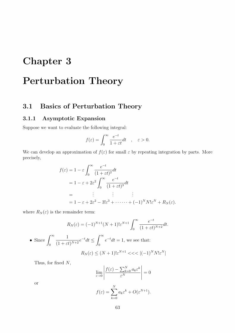
Chapter 3

Perturbation Theory

3.1 Basics of Perturbation Theory

3.1.1 Asymptotic Expansion

Suppose we want to evaluate the following integral:

f(ε) =

∫ ∞0

e−t

1 + εtdt , ε > 0.

We can develop an approximation of f(ε) for small ε by repeating integration by parts. Moreprecisely,

f(ε) = 1− ε∫ ∞

0

e−t

(1 + εt)2dt

= 1− ε+ 2ε2

∫ ∞0

e−t

(1 + εt)3dt

=...

......

= 1− ε+ 2ε2 − 3!ε3 + · · · · · ·+ (−1)NN !εN +RN(ε).

where RN(ε) is the remainder term:

RN(ε) = (−1)N+1(N + 1)!εN+1

∫ ∞0

e−t

(1 + εt)N+2dt.

• Since

∫ ∞0

1

(1 + εt)N+2e−tdt ≤

∫ ∞0

e−tdt = 1, we see that:

RN(ε) ≤ (N + 1)!εN+1 <<< |(−1)NN !εN |

Thus, for fixed N ,

limε→0

∣∣∣∣∣f(ε)−∑N

k=0 akεk

εN

∣∣∣∣∣ = 0

or

f(ε) =N∑k=0

akεk +O(εN+1).

63

64 3.1. Basics of Perturbation Theory

• The formal seriesN∑k=0

akεk is said to be an asymptotic expansion of f(ε) such that for

fixed N , it provides a good approximation of f(ε) as ε −→ 0.

• However, the expansion is not convergent for fixed ε since (−1)NN !εN −→ ∞ as N −→∞.

Definition 3.1.1 (Big O and Little O notation).

(a) f(ε) = O(g(ε)) as ε −→ 0 means that there exists M > 0 such that |f | ≤M |g| as ε −→ 0.

(b) f(ε) = o(g(ε)) as ε −→ 0 means that limε→0

∣∣∣∣f(ε)

g(ε)

∣∣∣∣ = 0.

Definition 3.1.2.

(a) The ordered sequence of functions δj(ε)∞j=0 is called an asymptotic sequence as ε −→ 0if δj+1(ε) = o(δj(ε)) as ε −→ 0.

• One example is the sequence 1, ε, ε2, · · · for small ε.

(b) Let f(ε) be a continuous function of ε, and δj(ε)∞j=0 be an asymptotic sequence. The

formal seriesN∑j=0

ajδj(ε) is called an asymptotic expansion of f(ε), valid to order δN(ε),

if for all N ≥ 0,

limε→0

∣∣∣∣∣f(ε)−∑N

j=0 ajδj(ε)

δN(ε)

∣∣∣∣∣ = 0.

• Usually write f(ε) ∼N∑j=0

ajδj(ε), ε −→ 0.

In the case of perturbation solution to an ODE, we will consider asymptotic expansions of

the form x(t, ε) ∼∑k

ak(t)δk(ε), which are valid over some interval of time. It is often useful

to characterise the time interval, i.e. we say that the estimate is valid on a time scale 1/δ(ε) ifthe following holds:

limε→0

∣∣∣∣∣x(t, ε)−∑N

k=0 ak(t)δk(ε)

δN(ε)

∣∣∣∣∣ = 0.

for 0 ≤ δ(ε) ≤ C, with C independent of ε.

Example 3.1.3. Suppose x(t, ε) = εt sin(t), x ∈ R, t ≥ 0, then

x(t, ε) = O(ε) for t = O(1).

x(t, ε) = O(1) for t ∼ 1

ε.

Perturbation Theory 65

3.1.2 Naive Expansions

Consider x = f(t, x; ε), x ∈ Rn, x(0) = x0. Suppose that we can expand f as a Taylor seriesin ε, i.e.

f(t, x; ε) = f0(t, x) + εf1(t, x) + · · · .One might expect a similar expansion exists for the solution:

x(t) = x0(t) + εx1(t) + ε2x2(t) + · · · .[δk(ε) = εk.

]Substitute this expansion into ODE and equate terms in equal powers of ε, this gives us anasymptotic approximation for t = O(1).

Example 3.1.4. Consider x+ 2εx+ x = 0, x(0) = a, x(0) = 0.

• This has explicit solution of the form:

x(t) = ae−εt cos(t√

(1− ε2))

+εa√

(1− ε2)e−εt sin

(t√

(1− ε2)).

There is 2 time scales here:

– The slowly decaying exponential which varies on time scale of1

ε.

– The oscillatory term which varies on time scale of 1.

• If we apply naive perturbation, we will pick up secular terms. More precisely,

e−εt cos(t√

(1− ε2))≈(

1− εt+ε2t2

2!

)cos(t).

• Alternatively, assume that an expansion exists for the solution and set

x(t) = x0(t) + εx1(t) + · · · .

Equating terms in equal powers of ε yields:

x0 + x0 = 0

......

...

xn + xn = −2xn−1 , n = 1, 2, · · · .

Solving these equations with initial conditions x0(0) = a, x0(0) = 0; xn(0) = 0, xn(0) = 0gives:

x0(t) = a cos(t)

x1(t) = a sin(t)− at cos(t).

– We see that x1(t) contains a secular term that grows linearly in t, making theasymptotic expansion valid for only small values of t.

– Another way to interpret this is that the solution breaks down when t ∼ 1

ε, since

εx1(t) will be of the same order as x0(t).

66 3.2. Method of Multiple Scales

3.2 Method of Multiple Scales

One often finds that solution oscillates on a time-scale of order t with an amplitude or phasethat drifts on a slower time-scale εt. This suggest we should look for solutions of the form

R(εt) sin(t+O(εt)).

or equivalentlyA(εt) sin(t) +B(εt) cos(t).

• In order to separate these time scales, we treat t and τ = εt as independent variables,and introduce the following asymptotic expansion:

X(t) = x(t, τ, ε) ∼ x0(t, τ) + εx1(t, τ) + · · .

which is asymptotic up to order 1/ε. In general, it might be√ε instead of ε

• τ = εt is called the slow time scale because it does not affect the asymptotic expansionuntil t is comparable with 1/ε.

• Using the chain rule, we have thatd

dt=

∂

∂t+ ε

∂

∂τ. Thus,

x =∂x0

∂t+ ε

∂x0

∂τ+ ε

[∂x1

∂t+ ε

∂x1

∂τ

]+ . . .

=∂x0

∂t+ ε

[∂x0

∂τ+∂x1

∂t

]+ . . .

x =

[∂2x0

∂t2+ ε

∂2x0

∂τ∂t

]+ ε

[∂2x0

∂t∂τ+ ε

∂2x0

∂τ 2

]+ ε

[∂2x1

∂t2+ ε

∂2x1

∂τ∂t

]+ . . .

=∂2x0

∂t2+ ε

[2∂2x0

∂t∂τ+∂2x1

∂t2

]+ . . .

Example 3.2.1. Consider the following initial value problem:x+ εx(x2 − 1) + x = 0.

x(0) = 1, x(0) = 0.

Suppose that X(t) has the asymptotic expansion of the form:

X(t) = x(t, ε, τ) ∼ x0(t, τ) + εx1(t, τ)

for t = O(1/ε). Substituting this expansion into the ODE and equate terms in equal powersof ε gives the following:

• Equation for O(1) term is: ∂2x0

∂t2+ x0 = 0.

x0(0, 0) = 1,∂x0

∂t(0, 0) = 0.

This has solution x0(t, τ) = R(τ) cos(t+ θ(τ)

), with R(0) = 1, θ(0) = 0. Note that the

constant might depends on τ . Also, when t = 0, so is τ .


• Equation for O(ε) term is:∂2x1

∂t2+ x1 = −2

∂2x0

∂t∂τ− ∂x0

∂t(x2

0 − 1).

x1(0, 0) = 0,

(∂x0

∂τ+∂x1

∂t

) ∣∣∣∣(0,0)

= 0.

– Substituting for x0 into the RHS yields:

−2∂2x0

∂t∂τ− ∂x0

∂t(x2

0 − 1) = −2∂

∂τ

[R sin(t+ θ)

]+R sin(t+ θ)

[R2 cos2(t+ θ)− 1

]= 2[Rθτ cos(t+ θ) +Rτ sin(t+ θ)

]+R sin(t+ θ)

[R2 cos2(t+ θ)− 1

]= 2[Rθτ cos(t+ θ) +Rτ sin(t+ θ)

]+R sin(t+ θ)

[R2(

1− sin2(t+ θ))− 1]

=[2Rτ +R(R2 − 1)

]sin(t+ θ) + 2Rθτ cos(t+ θ)

−R3 sin3(t+ θ).

– The first two terms are secular/resonant terms, which we need to eliminate. Fromthis, we obtain two initial value problems for R(τ) and θ(τ):

2Rτ = R(1−R2), R(0) = 1

θτ = 0, θ(0) = 0.

The second equation immediately implies that θ(τ) = 0 for all τ ≥ 0.

– In particular, we can solve for R(τ) explicitly by first using the substitution y = R2:

1 =2

R(1−R2)

dR

dτ

=2

R(1−R2)

(1

2R

dy

dτ

)=

1

y(1− y)

dy

dτ

=

[1

y+

1

1− y

]dy

dτ

Integrating both sides with respect to τ yields:

ln |y| − ln |1− y| = τ + A

τ + A = ln

∣∣∣∣ y

1− y

∣∣∣∣

68 3.3. Averaging Theorem: Periodic Case

3.3 Averaging Theorem: Periodic Case

3.4 Phase Oscillators and Isochrones


3.5 Problems

1. Consider the equationx+ x = −ε(x2 − x), 0 < ε 1.

Using the method of multiple scales, show that

x0(t, τ) = A(τ) +B(τ)e−t,

and identify any resonant terms at O(ε). Show that the non-resonance condition is

Aτ = A− A2,

and describe the asymptotic behaviour of solutions.

Solution:

2. Consider the Van der Pol equation

x+ x+ ε(x2 − 1)x = Γ cos(ωt), 0 < ε 1,

with Γ = O(1) and ω 6= 1

3, 1, 3. Using the method of multiple scales, show that the solution

is attracted to

x(t) =Γ

1− ω2cos(ωt) +O(ε)

when Γ2 ≥ 2(1− ω2)2 and

x(t) = 2

(1− Γ2

2(1− ω2)2

)1/2

cos(t) +Γ

1− ω2cos(ωt) +O(ε)

when Γ2 < 2(1− ω2)2. Explain why this result breaks down when ω =1

3, 1, 3.

Solution:

3. Consider the following differential equation

x+ x = −εf(x, x),

with |ε| 1. Let y = x.

(a) Show that if E(x, y) = (x2 + y2)/2, then E = −εf(x, y)y. Hence show that an approx-imate periodic solution of the form x = A cos(t) +O(ε) exists if∫ 2π

0

f(A cos(t),−A sin(t)) sin(t) dt = 0.

70 3.5. Problems

Solution:

(b) Let En = E(x(2πn), y(2πn)) and E0 = E(x(0), y(0)). Show that to lowest order Ensatisfies a difference equation of the form

En+1 − En + εF (En)

and write down F (En) explicitly as an integral. Hence deduce that a periodic orbitwith approximate amplitude A∗ =

√2E∗ exists if F (E∗) = 0 and this orbit is stable if

εdF

dE(E∗) < 0.

Hint : Spiralling orbits close to the periodic orbit x = A∗ cos(t) +O(ε) can be approx-imated by a solution of the form x = A cos(t) +O(ε).

Solution:

(c) Using the above result, find the approximate amplitude of the periodic orbit of the Vander Pol equation

x+ x+ ε(x2 − 1)x = 0,

and verify that it is stable.

Solution:

4. Consider the forced Duffing equation

x+ ω2x = ε[γ cos(ωt)− κx− βx− x3].

Using the method of averaging withx(t) = a(t) cos(ωt) +b(t)

ωsin(ωt)

x(t) = −a(t)ω sin(ωt) + b(t) cos(ωt),

derive dynamical equations for the amplitudes a, b and show that they are identical to theamplitude equations obtained using the method of multiple scales.

Solution:

Chapter 4

Boundary Value Problems

4.1 Compact Symmetric Linear Operators

Definition 4.1.1. Let V be a complex vector space. An inner product is a mapping 〈·, ·〉 : V×V −→ C with the following properties

(a) 〈αf1 + βf2, g〉 = α∗〈f1, g〉+ β∗〈f2, g〉 for all α, β ∈ C.

(b) 〈f, g〉 = 〈g, f〉∗.

(c) 〈f, f〉 = 0⇐⇒ f = 0.

Associated with every inner product is an associated norm ‖f‖ =√〈f, f〉. If V is complete

with respect to the above norm, then V is a Hilbert space.

Theorem 4.1.2 (Cauchy-Schwarz). |〈f, g〉| ≤ ‖f‖‖g‖.

Proof. The inequality is trivial if g = 0, so assume that g 6= 0. Define h = f − 〈f, g〉‖g‖

g. Since

〈h, g〉 = 0, Pythagorean theorem yields

‖f‖2 =

∥∥∥∥h+〈f, g〉g‖g‖

∥∥∥∥2

=

⟨h+〈f, g〉g‖g‖

, h+〈f, g〉g‖g‖

⟩= ‖h‖2 +

|〈f, g〉|2

‖g‖2

≥ |〈f, g〉|2

‖g‖2.

Lemma 4.1.3 (Bessel’s inequality). Suppose (uj) is an orthonormal sequence in a Hilbert spaceH. The following inequality holds for any f ∈ H

∞∑j=1

|〈uj, f〉|2 ≤ ‖f‖2.

71

72 4.1. Compact Symmetric Linear Operators

Proof. Suppose (uj) is an orthonormal sequence in H. Any f ∈ H can be written as

f = f⊥ +n∑j=1

〈uj, f〉uj.

Note that for any fixed k = 1, . . . , n,

〈uk, f⊥〉 =

⟨uk, f −

n∑j=1

〈uj, f〉uj

⟩= 〈uk, f〉 − 〈uk, f〉 = 0.

=⇒ ‖f‖2 = ‖f⊥‖2 +n∑

j,k=1

〈uj, f〉∗〈uk, f〉〈uj, uk〉

= ‖f⊥‖2 +n∑j=1

|〈uj, f〉|2

≥n∑j=1

|〈uj, f〉|2.

The result follows by taking limit as n −→∞.

Definition 4.1.4.

(a) A linear operator is a linear mapping A : D(A) −→ H, where H is a Hilbert space andD(A) is a linear subspace of H, called the domain of A.

(b) A linear operator A is symmetric if

(i) its domain is dense, that is, D(A) = H, and

(ii) 〈g, Af〉 = 〈Ag, f〉 for all f, g ∈ D(A).

(c) A number λ ∈ C is called an eigenvalue of a linear operator A if there exists a non-zerovector u ∈ D(A), called an eigenvector of λ such that Au = λu.

(d) An eigenspace is N (A− λI) =u ∈ D(A) : (A− λI)u = 0

.

Theorem 4.1.5. Let A be a symmetric linear operator. Then all eigenvalues of A (if theyexists) are real and eigenvectors of distinct eigenvalues are orthogonal.

Proof. Suppose λ is an eigenvalue with unit normalised eigenvector u.

λ = 〈u,Au〉 = 〈Au, u〉 = λ∗

This implies that λ is real. If Auj = λjuj, j = 1, 2, then

(λ1 − λ2)〈u1, u2〉 = 〈Au1, u2〉 − 〈u1, Au2〉 = 0.

since A is symmetric. Thus, if λ1 − λ2 6= 0, we must have 〈u1, u2〉 = 0 =⇒ u1 ⊥ u2.

Boundary Value Problems 73

Definition 4.1.6 (Boundedness and Compactness).

(a) A linear operator A with D(A) = H is said to be bounded if

‖A‖ = supf∈D(A),‖f‖=1

‖Af‖ <∞

– By construction, ‖Af‖ ≤ ‖A‖‖f‖, i.e. a bounded linear operator is continuous.

(b) A linear operator A with D(A) = H is said to be compact if for any bounded sequence(fn) ⊂ D(A), the sequence (Afn) has a convergent subsequence in H.

– It can be shown that every compact linear operator is bounded.

Theorem 4.1.7. A compact symmetric operator A has an eigenvalue λ0 for which |λ0| = ‖A‖.

Proof. The result is trivial is A = 0, so suppose not. Denote a = ‖A‖, with a 6= 0. Bydefinition of ‖A‖, we have that

‖A‖2 = sup‖f‖=1

‖Af‖2 = sup‖f‖=1

〈Af,Af〉 = sup‖f‖=1

〈f, A2f〉.

This implies that there exists a normalised sequence (un) such that limn→∞〈un, A2un〉 = a2. Since

A is compact, A2 is also compact, so there exists a subsequence (unk) such that A2unk −→ y =a2u in H as k −→∞ for some u ∈ H. Since A is symmetric,

‖(A2 − a2)unk‖2 = ‖A2unk‖2 − 〈A2unk , a2unk〉 − 〈a2unk , A

2unk〉+ ‖a2unk‖2

= ‖A2unk‖2 − 2a2〈unk , A2unk〉+ a4‖unk‖2

≤ (a2)2‖unk‖2 − 2a2〈unk , A2unk〉+ a4‖unk‖2[A is bounded

]= 2a4 − 2a2〈unk , A2unk〉

[‖unk‖2 = 1

]= 2a2

[a2 − 〈unk , A2unk〉

]−→ 0 as k −→∞

Hence, we have

‖a2unk − a2u‖ ≤ ‖a2unk − A2un‖+ ‖A2unk − a2u‖−→ 0 as k −→∞.

which implies that unk −→ u in D(A) = H as k −→∞. It follows that

0 = limk→∞

(A2 − a2)unk = (A2 − a2)u = (A+ aI)(A− aI)u,

There are two possible cases

1. Either (A− aI)u = 0 =⇒ λ0 = a,

2. or (A− aI)u = v 6= 0 and (A+ aI)v = 0, which gives λ0 = −a.

74 4.1. Compact Symmetric Linear Operators

Remark 4.1.8. A bounded operator cannot have an eigenvalue |λ| > ‖A‖ since

|λ|‖u‖ = ‖λu‖ = ‖Au‖ ≤ ‖A‖‖u‖.

Theorem 4.1.9 (Spectral Theorem for Compact Symmetric Linear Operators).Suppose H is a Hilbert space and A : H −→ H is a compact symmetric linear operator.

(a) There exists a sequence of real eigenvalues (λn)∞n=0 −→ 0. The corresponding normalisedeigenvectors u0, u1, . . . form an orthornormal set in H.

(b) Every f ∈ R(A) can be written as

f =N∑j=0

〈uj, f〉uj. (4.1.1)

(c) If R(A) is dense in H, then the set of normalised eigenvectors form an orthonormal basisof H.

Proof. We first establish existence of an orthonormal set of eigenvectors (eigenfunctions) usingTheorem 4.1.7.

• Let H(0) = H and A0 = A|H(0) : H(0) −→ H(0). From Theorem 4.1.7, there exists aneigenvalue λ0 and a normalised eigenvector u0 ∈ H(0) such that

Au0 = λ0u0, with |λ0| = ‖A0‖ = ‖A‖.

• Define H(1) := (span(u0))⊥ = f ∈ H : 〈f, u0〉 = 0. Note that H(1) ⊂ H(0).

– Since A is symmetric, for any f ∈ H(1) we have that

〈Af, u0〉 = 〈f, Au0〉 = λ0〈f, u0〉 = 0.

This means that Af ∈ H(1).

– Let A1 = A|H(1) : H(1) −→ H(1) be the restriction of A to H(1), this is again acompact symmetric linear operator. From Theorem 4.1.7, there exists an eigenvalueλ1 and a normalised eigenvector u1 ∈ H(1) such that

A1u1 = λ1u1, with |λ1| = ‖A1‖.

Moreover, we have that 〈u1, u0〉 = 0 since u1 ∈ H(1).

By iterating this argument, we construct a family of spaces H(n) and compact symmetric lin-ear operators A(n), together with a sequence of eigenvalues (λj) with corresponding normalisedeigenvectors (uj), satisfying

1. . . . H(n) ⊂ H(n−1) ⊂ . . . ⊂ H(0) = H.

2. H(n) =[span(u0, · · · , un−1)

]⊥for all n ≥ 1.


3. An : H(n) −→ H(n), with Anun = λnun and |λn| = ‖An‖ for each n ≥ 0.

Moreover, the nested property of H(n) implies that 〈uk, uj〉 = 0 for all 0 ≤ k < j. Thisiterative procedure does not terminate unless R(A) is finite-dimensional. Indeed, if R(A) is ofdimension n <∞, then

An = A|H(n) = 0 =⇒ λj = 0 for all j ≥ n.

Now, suppose λj 6−→ 0. There exists a subsequence λjk and ε > 0 such that |λjk | > ε for

all k ≥ 1. Consider the sequence (vk) defined by vk =ujkλjk

, which is well-defined since λjk 6= 0.

Observe that (vk) is a bounded sequence since (ujk) has unit norm and (λjk) is bounded below.Moreover, for any k 6= l we have that

‖Avk − Avl‖2 =∥∥∥Aujkλjk− Aujl

λjl

∥∥∥2

= ‖ujk − ujl‖2[since Aun = λnun

]= ‖ujk‖2 + ‖ujl‖2

[since 〈um, un〉 = δmn

]= 2

[since ‖un‖ = 1

]Thus, any subsequence of (Avk) is not a Cauchy sequence and does not converge. This contra-dicts the compactness of the linear operator A since (vk) is a bounded sequence.

Next, let f = Ag ∈ R(A), and denote fn =n∑j=0

〈uj, f〉uj. Observe that

fn =n∑j=0

〈uj, f〉uj =n∑j=0

〈uj, Ag〉uj

=n∑j=0

〈Auj, g〉uj[since A is symmetric

]=

n∑j=0

λ∗j〈uj, g〉uj

=n∑j=0

λj〈uj, g〉uj[from Theorem 4.1.5

]=

n∑j=0

〈uj, g〉Auj[since Auj = λjuj

]= A

[n∑j=0

〈uj, g〉uj

] [since A is linear

]= Agn.

For any k = 0, . . . , n, we also have that

〈uk, g − gn〉 = 〈uk, g〉 −

⟨uk,

n∑j=0

〈uj, g〉uj

⟩= 〈uk, g〉 − 〈uk, g〉 = 0,

76 4.2. Linear Differential Operators

i.e. g − gn ∈[span(u0, · · · , un)

]⊥= H(n+1). There are two possible cases:

1. dim(R(A)) = n+ 1 <∞.

This means that An+1 = 0. Since g − gn ∈ H(n+1), we have that

f − fn = Ag − Agn = A(g − gn) = An+1(g − gn) = 0.

2. dim(R(A)) =∞.

Since g − gn ∈ H(n+1), Pythagorean theorem yields

‖g‖2 = ‖g − gn + gn‖2 = ‖g − gn‖2 + ‖gn‖2 ≥ ‖g − gn‖2.

Boundedness of An+1 gives

‖f − fn‖2 = ‖An+1(g − gn)‖2 ≤ ‖An+1‖2‖g − gn‖2 ≤ |λn+1|2‖g‖2 −→ 0 as n −→∞.

In both cases, we prove that fn −→ f and so (4.1.1) holds.

Finally, let f ∈ H and supposeR(A) is dense in H. Given any ε > 0, there exists fε ∈ R(A)such that ‖f − fε‖ < ε. Moreover, from previous step, there exists fε ∈ span(u0, · · · , un) forsufficiently large n such that ‖fε − fε‖ < ε. Thus,

‖f − fε‖ ≤ ‖f − fε‖+ ‖fε − fε‖ < 2ε

for sufficiently large n.

Remark 4.1.10. We would like to carry out a similar analysis to derive a spectral theoremfor differential operator. The problem is that symmetric differential operator are not compact,or even bounded. Fortunately, one can construct an inverse of a differential operator that iscompact (Green’s functions and integral equations).

4.2 Linear Differential Operators

Consider the formal linear differential operator on [a, b] ⊂ R defined by

L = p0(x)dn

dxn+ p1(x)

dn−1

dxn−1+ . . .+ pn(x). (LDO)

where we are not concerned about the space of functions it is applied to. A natural choiceof function space is the Hilbert space L2[a, b], since we can work with inner product andorthogonality.

• First, note that L cannot act on all functions in L2[a, b] because not all of them aredifferentiable. Because of this, we require that our domain D(L) contains only functionsthat are sufficiently differentiable, but the image of these functions under L need only bein L2[a, b].

• Usually, we further restrict D(L) by imposing boundary conditions at the endpoints ofthe interval. The boundary conditions that we will impose will always be linear andhomogeneous, this will make D(L) a vector space.


4.2.1 Formal Adjoint

With the above linear differential operator L, consider a weight function ω(x) which is definedto be a real and positive function on (a, b). We can construct another operator L† such thatthe following holds for any smooth function u(x), v(x)

ω[u∗Lv − (L†u)∗v

]=

d

dx

(Q[u, v]

), (4.2.1)

for some function Q[·, ·] that depends bilinearly on its arguments and their first n− 1 deriva-tives. (4.2.1) is called the Lagrange’s identity and L† is called the formal adjoint of L withrespect to the weight function ω. Note that we are yet to specify D(L†).

Now, consider a weighted inner product defined by

〈u, v〉ω =

∫ b

a

ωu∗v dx.

If u and v have boundary conditions such that Q[u, v]|ba = 0, then

〈u, Lv〉ω = 〈L†u, v〉ω

which looks similar to how we define an adjoint operator on a normed vector space! A commonmethod for finding the formal adjoint is using integration by parts.

Example 4.2.1 (Sturm-Liouville operator). Consider the following linear differential operator

L = p0(x)d2

dx2+ p1(x)

d

dx+ p2(x),

where pj(x) are all real and ω(x) ≡ 1. Integrating by parts twice yields

〈u, Lv〉 =

∫ b

a

u∗(x)

[p0(x)

d2v

dx2+ p1(x)

dv

dx+ p2(x)v(x)

]dx

=

[u∗(x)p0(x)

dv

dx

] ∣∣∣∣ba

−∫ b

a

d

dx

(p0(x)u∗(x)

)dvdx

dx

+

[u∗(x)p1(v)v(x)

]∣∣∣∣ba

−∫ b

a

d

dx

(p1(x)u∗(x)

)v(x) dx

+

∫ b

a

u∗(x)p2(x)v(x) dx

=

∫ b

a

[d2

dx2

(p0(x)u(x)

)− d

dx

(p1(x)u(x)

)+ p2(x)u(x)

]∗v(x) dx

+

[u∗(x)p0(x)

dv

dx− d

dx

(p0(x)u∗(x)

)v(x) + u∗(x)p1(x)v(x)

] ∣∣∣∣ba

Thus, we see that

L† =d2

dx2p0 −

d

dxp1 + p2


= p0d2

dx2+ (2p′0 − p1)

d

dx+ p′′0 − p′1 + p2.

In order for L to be formally self-adjoint, we choose2p′0 − p1 = p1 =⇒ p′0 = p1

p′′0 − p′1 + p2 = p2 =⇒ p′′0 = p′1 =⇒ p′0 = p1

Thus, by choosing p1 = p′0, we have the well-known Sturm-Liouville operator given by

L =d

dx

(p0(x)

d

dx

)+ p2(x).

Remark 4.2.2. What happens if p1 6= p′0? We can still make L formally self-adjoint bychoosing a suitable weight function ω(x). Suppose p0(x) is positive definite on (a, b), i.e.p0(x) > 0 and pj(x) are all real. Define

ω(x) =1

p0(x)exp

[∫ x

a

p1(x′)

p0(x′)dx′].

We can rewrite L in the following form

Lu =1

ω

d

dx

(ωp0

du

dx

)+ p2u.

One can show that L† = L. Thus, as long as p0(x) 6= 0, we can always define a weightedinner product in which a real second-order differential operator is formally self-adjoint withrespect to this weighted inner product.

4.2.2 A Simple Eigenvalue Problem

Recall that a finite self-adjoint (Hermitian) matrix has a complete set of orthonormal eigen-vectors. Does the same property hold for self-adjoint differential operators?

Example 4.2.3. Consider the differential operator L = − d2

dx2, with domain

D(L) =f, Lf ∈ L2[0, 1] : f(0) = f(1) = 0

.

Integrating by parts yields

〈f1, Lf2〉 =

∫ 1

0

f ∗1

(−d

2f2

dx2

)dx

=

∫ 1

0

(−d

2f1

dx2

)∗f2 dx+

[− f ∗1 f ′2 + (f ∗1 )′f2

]∣∣∣∣10

= 〈Lf1, f2〉

We see that L is self-adjoint with the given boundary conditions.

The eigenvalue equation Lψ = λψ ord2ψ

dx2+ λψ = 0, with the boundary conditions ψ(0) =

ψ(1) = 0 has solutions ψn(x) = sin(nπx) with eigenvalues λn = n2π2. Observe that


1. The eigenvalues are real.

2. The eigenfunctions are orthogonal, that is

2

∫ 1

0

sin(mπx) sin(nπx) dx = δmn.

3. The normalised eigenfunctions are complete, i.e. any f ∈ L2[0, 1] can be written as anL2 convergent series of the following form

f(x) =∞∑n=1

an√

2 sin(nπx).

Example 4.2.4. Consider the differential operator L = −i ddx

, with domain

D(L) =f, Lf ∈ L2[0, 1] : f(0) = f(1) = 0

.

We claim that L is self-adjoint. Indeed, integrating by parts gives

〈f1, Lf2〉 =

∫ 1

0

f ∗1

(−idf2

dx

)dx

=

[− if ∗1 f2

]∣∣∣∣10

+ i

∫ 1

0

df ∗1dx

f2 dx

= 〈Lf1, f2〉.

On the other hand, the eigenvalue equation −idψdx

= λψ ordψ

dx= iλψ has solution ψ(x) ∼ eiλx.

However, ψ(x) does not satisfy the boundary conditions as exponential function is a positive

function. Thus, L = −i ddx

doesn’t have an eigenvalue! This suggest that the problem lies in

the boundary conditions.

4.2.3 Adjoint Boundary Conditions

To rectify the problem, we remove the requirement that D(L) = D(L†), but still ensuring thatD(L†) is defined such that Q[u, v] = 0 in (4.2.1). More precisely, given v ∈ D(L) satisfyingcertain boundary conditions, we impose any required boundary conditions on u ∈ D(L†) suchthat Q[u, v] = 0 in (4.2.1). Such boundary conditions on u ∈ D(L†) are called the adjointboundary conditions and they define D(L†).


, with domain

D(L) =f, Lf ∈ L2[0, 1] : f(1) = 0

.

From previous computation, we find that

〈u, Lv〉 − 〈L†u, v〉 = −i[u∗(1)v(1)− u∗(0)v(0)

]


The first term vanishes since v(1) = 0. Because v(0) can take any value, we must chooseu(0) = 0 in order for Q[u, v] to vanish. Imposing this boundary condition on u ∈ D(L†) thus

yields L† = L = −i ddx

and

D(L†) =f, Lf ∈ L2[0, 1] : f(0) = 0

.

We remark that although L is formally self-adjoint, L,L† are not the same operator sinceD(L) 6= D(L†). We then say that L is not truly self-adjoint.

Example 4.2.6. Consider the same differential operator L = −i ddx

, but now with a different

domainD(L) =

f, Lf ∈ L2[0, 1] : f(0) = f(1) = 0

.

It is clear that Q[u, v] = 0 irrespective of any boundary conditions on u. That is, there is noconstraint on u. Thus, L† = L and

D(L†) =f, Lf ∈ L2[0, 1]

.

Again, L is not truly self-adjoint since D(L) 6= D(L†).

4.2.4 Self-Adjoint Boundary Conditions

Definition 4.2.7. A formally self-adjoint operator L is truly self-adjoint if and only if L = L†

and D(L) = D(L†). Thus, one needs to impose self-adjoint boundary conditions in orderto obtain a self-adjoint operator.


. We investigate what boundary

conditions we need to impose so that L is truly self-adjoint. Previous calculation shows that

〈u, Lv〉 − 〈Lu, v〉 = −i[u∗(1)v(1)− u∗(0)v(0)

].

Demanding the right hand side vanishes gives us the condition

u∗(1)

u∗(0)=v(0)

v(1).

We require this to be true for any u, v obeying the same boundary conditions.

Since u, v are not a-priori related, it follows that

u∗(1)

u∗(0)= Λ =

v(0)

v(1).

Since we require that both u, v belong to the same domain, we also have

Λ∗ =u(1)

u(0)=v(1)

v(0)= Λ−1.


i.e. Λ∗ = Λ−1 =⇒ Λ = eiθ for some real phase θ ∈ R. The domain is therefore

D(L) =f, Lf ∈ L2[0, 1] : f(1) = eiθf(0)

.

These are called twisted periodic boundary conditions. With this self-adjoint boundaryconditions, everything is groovy:

1. The eigenfunctions are ψn(x) = e(2πn+θ)ix with eigenvalues λn = 2πn+ θ.

2. The eigenvalues are real and the normalised eigenfunctions (ψn) form a complete or-thonormal set.

Example 4.2.9. Consider the Sturm-Liouville differential operator defined by

L =d

dx

(p(x)

d

dx

)+ q(x), x ∈ [a, b].

We shown previously that this is formally self-adjoint, satisfying

〈u, Lv〉 − 〈Lu, v〉 =

[p(u∗v′ − (u∗)′v

)]∣∣∣∣ba

.

As before, demanding the right hand side vanishes gives us conditions at both ends:

(u∗)′(a)

u∗(a)=v′(a)

v(a),

(u∗)′(b)

u∗(b)=v′(b)

v(b).

To ensure D(L) = D(L†), we also require that

v′(a)

v(a)=u′(a)

u(a)= Λa,

v′(b)

v(b)=u′(b)

u(b)= Λb.

Comparing these two conditions, we thus require that Λa = Λ∗a and Λb = Λ∗b , i.e. Λa,Λb ∈ R.Thus, we have the following self-adjoint boundary conditions:

Λaf(a)− f ′(a) = 0

Λbf(b)− f ′(b) = 0.

4.3 Eigenvalue Problems and Spectral Theory

It can be proven that a truly self-adjoint operator T with respect to L2[a, b] inner productposseses a complete set of mutually orthogonal eigenfunctions. The set of eigenvalues belongto the spectrum of T , denoted σ(T ). It forms the point spectrum provided their correspond-ing eigenfunctions belong to L2[a, b]. Usually, the eigenvalues of the point spectrum form adiscrete set, so the point spectrum is also known as the discrete spectrum. When a differen-tial operator acts on functions on R, the functions may fail to be normalisable; the associatedeigenvalues then belong to the continuous spectrum. The spectrum maybe partially dis-crete and partially continuous. There can also be a residual spectrum, but this is empty forself-adjoint operators.

82 4.3. Eigenvalue Problems and Spectral Theory

4.3.1 Discrete Spectrum

Let T be a self-adjoint linear operator on a bounded domain [a, b]. The eigenvalue equation is

Tφn(x) = λnφn(x)

for integer n ∈ Z. We also imposed the normalised condition∫ b

a

φ∗n(x)φm(x) dx = δnm.

Completeness of these eigenfunctions can be expressed by the following condition∑n∈Z

φn(x)φ∗n(y) = δ(x− y), (4.3.1)

where convergence is understood in the sense of distributions. More precisely, in order to makesense of this notion of convergence, we have to multiply (4.3.1) by a smooth test functionf(y) and integrate with respect to y, which gives

f(x) =∑n∈Z

φn(x)

∫ b

a

φ∗n(y)f(y) dy =∑n∈Z

anφn(x),

where an =

∫ b

a

φ∗n(x′)f(x′)dx′. The upshot is we can expand any L2 functions if we can repre-

sent a delta function in terms of the eigenfunctions φn(x).

4.3.2 Continuous Spectrum

Consider the linear differential operator H = − d2

dx2on

[−L

2,L

2

]. This operator has eigenfunc-

tions φk(x) = eikx corresponding to eigenvalues λk = k2. Suppose we impose periodic boundaryconditions at x = ±L/2. This means that

φk(−L/2) = φk(L/2) =⇒ k = kn =2πn

L, n ∈ Z.

To find the normalised eigenfunctions,∫ L/2

−L/2φ∗n(x)φm(x) dx =

∫ L/2

−L/2ei

2πL

(m−n)x dx =

L if m = n,

0 if m 6= n.=⇒ φn(x) =

1√Leiknx.

Referring to (4.3.1), the completeness condition is

∞∑n=−∞

1

Leiknxe−ikny = δ(x− y), x, y ∈

[−L

2,L

2

].

As L −→ ∞, the eigenvalues become so close together, they can no longer be distinguishedand σ(H) −→ R. Moreover, the sum over n becomes an integral

∞∑n=−∞

1

Leiknxe−ikny −→

∫ (1

Leikxe−iky

)dn =

∫ (1

Leikxe−iky

)(dn

dk

)dk,


wheredn

dk=

L

2πis called the density of states. Note that

dn

dkis the Radon-Nikodym

derivative, i.e. it is a ratio of measures. Thus, in the limit as L −→ ∞, the completenesscondition becomes: ∫ ∞

−∞eik(x−y) dk

2π= δ(x− y).

When L =∞, φk(x) ∼ eikx is no longer normalisable on L2(R) since∫ ∞−∞

φ∗k(x)φk(x) dx =

∫ ∞−∞

e−ikxeikx dx =

∫ ∞−∞

dx =∞!

Strictly speaking, φk(x) is not a true eigenfunction and points in the continuous spectrum arenot actually eigenvalues. More rigorously, a point λ lies in the continuous spectrum if for anyε > 0, there exists an approximate eigenfunction φε ∈ L2(R) such that ‖φε‖ = 1 and‖Hφε− λφε‖ < ε. In other words, the inverse operator (resolvent) (H − λI)−1 is unbounded.

4.3.3 Mixed Spectrum

Consider the following eigenvalue equation, known as the Poschel-Teller equation

Hψ =

[− d2

dx2− 2sech2(x)

]ψ = λψ, x ∈ R.

We try a solution of the form ψk(x) =[a+ btanh(x)

]eikx. This gives

[− d2

dx2− 2sech2(x)

]ψk(x) = k2ψk(x)− 2(ikb+ a)sech2(x)eikx.

Thus, Hψk = k2ψk provided ikb+ a = 0 =⇒ ψk(x) = b[− ik + tanh(x)

]eikx.

For k 6= 0, the formal normalised eigenfunctions are

ψk(x) =1√

1 + k2eikx[− ik + tanh(x)

].

It is constructed in such a way that

ψk(x)ψ∗k(x′) =

1√1 + k2

eikx[− ik + tanh(x)

] 1√1 + k2

e−ikx′[ik + tanh(y)

]=

1

1 + k2eik(x−x′)

[− ik + tanh(x)

][ik + tanh(x′)

]−→ 1

1 + k2eik(x−x′)(−ik + 1)(ik + 1) as |x| −→ ∞

=1 + k2

1 + k2eik(x−x′) = eik(x−x′).


Thus, σ(H) contains a continuous part with λk = k2 and ψk(x) as “eigenfunctions”. For thespecial case λk = 0,

d2ψ0(x)

dx2= −2sech2(x)ψ0(x) =⇒ ψ0(x) =

1√2

sech(x).

This is normalisable, i.e. λ0 = 0 belongs to the discrete spectrum.

Let us compute the difference:

I = δ(x− x′)−∫ ∞−∞

ψk(x)ψ∗k(x′)dk

2π=

∫ ∞−∞

[eik(x−x′) − ψk(x)ψ∗k(x

′)] dk

2π

=

∫ ∞−∞

eik(x−x′)

1 + k2

[(1 + k2)− k2 + ik

(tanh(x′)− tanh(x)

)− tanh(x)tanh(x′)

]dk2π.

It can be shown (by residue theorem) that∫ ∞−∞

(eik(x−x′)

1 + k2

)dk

2π=

1

2e−|x−x

′|

∫ ∞−∞

(eik(x−x′)ik

1 + k2

)dk

2π= −1

2e−|x−x

′|sgn(x− x′).

Hence, I =1

2

[1 − sgn(x − x′)

(tanh(x′) − tanh(x)


]e−|x−x

′|. WLOG, take

x > x′. Then

I =1

2

[1−

(tanh(x′)− tanh(x)


]e−(x−x′)

=1

2

[1 + tanh(x)− tanh(x′)− tanh(x)tanh(x′)

]e−(x−x′)

=1

2

[1 + tanh(x)

][1− tanh(x′)

]e−(x−x′)

=1

2sech(x)sech(x′)

= ψ0(x)ψ0(x′).

Thus, we have the completeness condition

ψ0(x)ψ0(x′) +

∫ ∞−∞

ψ∗k(x)ψk(x′)dk

2π= δ(x− x′).

4.3.4 Rayleigh-Ritz Variational Principle

Consider the Sturm-Liouville operator

Lφ = − d

dx

(pdφ

dx

)+ qφ, x ∈ [a, b], (4.3.2)


together with self-adjoint boundary conditions

αφ(a) + βφ′(a) = 0 (4.3.3a)

αφ(b) + βφ′(b) = 0. (4.3.3b)

where p, q are real-valued functions. Suppose the following two statements hold:

1. There exists a countable infinite set of eigenvalues (λn) of (4.3.2) that are real-valuedand non-negative such that

0 ≤ λ1 ≤ λ2 ≤ λ3 ≤ . . . . . .

2. The corresponding eigenfunctions form a complete orthonormal set.

〈φn, φm〉 =

∫ b

a

φ∗n(x)φm(x) dx = δmn.

Using these, we derive a variational principle characterising eigenvalues of (4.3.2).

Consider a sufficiently smooth, bounded function u with the following properties:

u(x) =∑k∈Z+

ukφk(x), uk = 〈u, φk〉, ‖u‖2 = 1. (4.3.4)

Introducing the energy integral E[u] = 〈u, Lu〉. Substituting the Fourier series expansion(4.3.4) of u into E[u] yields

E[u] = 〈u, Lu〉 =

∫ b

a

[ ∑k∈Z+

u∗kφ∗k(x)

]L

[ ∑j∈Z+

ujφj(x)

]dx

=∑k,j∈Z+

u∗kuj

[∫ b

a

φ∗k(x)(Lφj(x)

)]dx

=∑k,j∈Z+

u∗kuj

∫ b

a

φ∗k(x)λjφj(x) dx

=∑k,j∈Z+

u∗kuj

[λj〈φk, φj〉

]=∑k∈Z+

λk|uk|2.

From the ordering of the eigenvalues,

E[u] =∑k∈Z+

λk|uk|2 ≥ λ1

∑k∈Z+

|uk|2 = λ1

∑k∈Z+

|〈u, φk〉|2 = λ1‖u‖2 = λ1,

where we use the Parseval’s identity and the assumption that all eigenvalues are non-negative. We see that the smallest eigenvalue λ1 is obtained by minimising E[u] with respectto all admissible functions u satisfying ‖u‖2 = 1. Moreover, a minimum occurs at u = φ1, since

E[φ1] =∑k∈Z+

λk|〈φ1, φk〉|2 = λ1.


Observe that by normalising all functions u ∈ D(L) and thus relaxing the constraint ‖u‖2 =1, the problem of finding the smallest eigenvalue λ1 is equivalent to the following minimisationproblem, called the Rayleigh quotient

λ1 = infu∈D(L)

〈u, Lu〉〈u, u〉

.

Similarly, if we restrict the class of admissible functions by requiring u also satisfying uk =〈u, φk〉 = 0 for all k = 1, 2, . . . , n− 1, i.e. u is orthogonal to lower eigenfunctions, then

E[u] =∞∑j=n

λj|uj|2 ≥ λn.

By defining Vn = span(φ1, φ2, . . . , φn−1), the problem of finding the nth eigenvalue λn is equiv-alent to the following minimisation problem

λn = infu∈D(L),u∈V ⊥n

〈u, Lu〉〈u, u〉

.

Of course, all of these are true with the assumptions that all eigenvalues are non-negative andtheir corresponding eigenfunctions form a complete orthonormal set. We now show that thisis indeed the case for the Sturm-Liouville eigenvalue problem.

Theorem 4.3.1. For the Sturm-Liouville operator L = − d

dx

(p(x)

d

dx

)+ q(x) with p, q non-

negative real-valued functions, we have the following results:

(a) The eigenvalues λn −→∞ as n −→∞.

(b) The corresponding eigenfunctions (φn) form a complete orthonormal set.

Proof. We now use the variational principle that we just developed to prove these two state-ments. For simplicity, consider the Dirichlet boundary condition, i.e. u(a) = u(b) = 0.

(a) Assuming u is real. Expanding E[u] and integrating by parts gives

E[u] = 〈u, Lu〉 =

∫ b

a

u∗Ludx

=

∫ b

a

u[− (pu′)′ + qu

]dx

=

∫ b

a

[pu′2 + qu2

]dx−

[u∗pu′

]∣∣∣ba

=

∫ b

a

[pu′2 + qu2

]dx.

where the boundary term vanishes. Consider the following expression

E[u]

‖u‖2=

∫ b

a

[pu′2 + qu2

]dx∫ b

a

u2 dx

,


and denote the following quantity

pM = maxx∈[a,b]

p(x), qM = maxx∈[a,b]

q(x)

pm = minx∈[a,b]

p(x), qm = minx∈[a,b]

q(x)

Replacing p(x), q(x) by the constant pM , qM , we obtain the following modified RayleighQuotient

EM [u]

‖u‖2≥ E[u]

‖u‖2=⇒ λ(M)

n ≥ λn.

Similarly, replacing p(x), q(x) by the constant pm, qm, we obtain the other modifiedRayleigh Quotient

Em[u]

‖u‖2≤ E[u]

‖u‖2=⇒ λ(m)

n ≤ λn.

Combining these two inequalities gives λ(m)n ≤ λn ≤ λ

(M)n .

Now, consider two intervals Im, IM such that Im ⊂ [a, b] ⊂ IM .

• Consider the variational problem forEM [u]

‖u‖2on Im. The admissible functions u must

now vanish on ∂Im, making the space of admissible functions smaller. This additionalconstraint implies that λ

(M)n ≤ λ

(M)n .

• Similarly, consider the variational problem forEm[u]

‖u‖2on IM . The admissible functions

u do not have to vanish at x = a, b, making the space of admissible function larger.This implies that λ

(m)n ≤ λ

(m)n .

In summary, we have the hierarchy

λ(m)n ≤ λ(m)

n ≤ λn ≤ λ(M)n ≤ λ(M)

n . (4.3.5)

The eigenvalues λ(m)n and λ

(M)n can be solved exactly since we have a constant coefficient

ODE. We find that both λ(m)n , λ

(M)n −→∞ as n −→∞. Hence, λn −→∞ as n −→∞.

(b) Consider the orthonormal set of eigenfunctions (φk), they satisfy the eigenvalue equationand boundary conditions

Lφk = − d

dx

(p(x)

dφkdx

(x)

)+ q(x)φk(x), φk(x) = 0 at x = a, b.

Define the remainder term Rn(x) = u(x)−n∑k=1

ukφk, with uk = 〈u, φk〉. We need to show

that limn→∞

‖Rn(x)‖ = 0. Since u(x) and φk(x) are admissable functions for the variational

problem, so is the remainder Rn(x). For all j = 1, . . . , n,

〈Rn, φj〉 =

⟨u−

n∑k=1

ukφk, φj

⟩= 〈u, φj〉 −

n∑k=1

u∗k〈φk, φj〉 = 0. (4.3.6)


By construction, we then have

E[Rn]

〈Rn, Rn〉≥ λn+1 =⇒ ‖Rn‖2 ≤ E[Rn]

λn+1

.

We have just shown that λn+1 −→ ∞ as n −→ ∞, so ‖Rn‖ −→ 0 as n −→ ∞ providedE[Rn] is uniformly bounded in n.

Let Ωn =n∑k=1

ukφk. Then

E[u] = E[Rn + Ωn]

= 〈Rn + Ωn, L(Rn + Ωn)〉= 〈Rn, LRn〉+ 〈Rn, LΩn〉+ 〈Ωn, LRn〉+ 〈Ωn, LΩn〉= E[Rn] + E[Ωn] + 〈LRn,Ωn〉+ 〈Ωn, LRn〉= E[Rn] + E[ΩN ] + 2Re(〈LRn,Ωn〉)= E[Rn] + E[Ωn] + 2〈LRn,Ωn〉

where we use the self-adjointness of L on the fourth equality and the assumption thatu, p, q are all real-valued functions. By repeating integration by parts,

〈LRn,Ωn〉 =

⟨LRn,

n∑k=1

ukφk

⟩=

n∑k=1

uk〈LRn, φk〉

〈LRn, φk〉 =

∫ b

a

(− (pR′n)′ + qRn

)φk dx

=[− pR′nφk

]∣∣∣ba

+

∫ b

a

(pR′nφ

′k + qRnφk

)dx

=[− pR′nφk +Rnpφ

′k

]∣∣∣ba

+

∫ b

a

(−Rn(pφ′k)

′ +Rnqφk

)dx

Because the Dirichlet boundary condition is homogeneous, D(L) is a vector space. Thus,φk(x), u(x) ∈ D(L) =⇒ Rn(x) ∈ D(L) and we immediately see that the boundary termvanishes. We are left with∫ b

a

(−Rn(pφ′k)

′ + qRnφk

)dx =

∫ b

a

Rn

(− (pφ′k)

′ + qφk

)dx

= λk

∫ b

a

Rnφk dx

= λk〈Rn, φk〉 = 0,

which follows from (4.3.6) since 1 ≤ k ≤ n. Thus, 〈LRn,Ωn〉 = 0 and

E[Rn] = E[u]− E[Ωn]

= E[u]− E

[n∑k=1

ukφk

]


= E[u]−∫ b

a

(n∑k=1

u∗kφ∗k

)L

(n∑j=1

ujφj

)dx

= E[u]−n∑

k,j=1

u∗kuj〈φk, Lφj〉

= E[u]−n∑

k,j=1

u∗kujλj〈φk, φj〉

= E[u]−n∑k=1

λk|uk|2

≤ E[u],

where we crucially use the fact that λk ≥ 0 for all k ≥ 1. Since u is an admissible function,E[u] is a finite value. Hence, E(Rn) is uniformly bounded in n, and we conclude that‖Rn‖ −→ 0 as n −→∞.

Remark 4.3.2. Let us justfiy the eigenvalue inequality (4.3.5) we proved in the first part ofthe theorem.

1. It seems like a lower bound of the form λ(m)n ≤ λn is sufficient. Indeed, this inequality

tells us that λ(m)n −→ ∞ as n −→ ∞ =⇒ λn −→ ∞ as n −→ ∞. However, it doesn’t

guarantee that λn <∞ for finite n.

2. The upper bound now comes into play. Now, we have the following inequality:

λ(m)n ≤ λn ≤ λ(M)

n

If additionally, we have that λ(M)n −→ ∞ as n −→ ∞, this “sandwich” guarantees that

λn <∞ for arbitrary but finite n.

3. Why is the inequality λ(m)n ≤ λn ≤ λ

(M)n not enough then? We are implicitly assuming

that we can show λ(m)n , λ

(M)n −→ ∞ as n −→ ∞. In general (even in 2D), they can be

really difficult to solve explicitly!

4.4 Distribution

In this section, we explore the analogy between matrices and linear operators on infinite-dimensional spaces. In the case of a finite-dimensional space, we choose a basis set and representthe linear operator in terms of the action of a matrix A ∈ Rm×n, i.e.

y = Ax or yi =n∑j=1

Aijxj, 1 ≤ i ≤ m.

Formally speaking, the function space analogue of this, g = Af , is

g(x) =

∫ b

a

A(x, y)f(y) dy,

90 4.4. Distribution

where we replace the summation over j by integration over a dummy variable y. If A(x, y) isan ordinary function, then A(x, y) is called an integral kernel. The Dirac delta functionis the analogue of identity operator in infinite-dimensional vector spaces.

f(x) =

∫ b

a

δ(x− y)f(y) dy.

Note that δ(x−y) is not an ordinary function, it is actually a generalised function/distributionas we will see later.

4.4.1 Distributions and Test Functions

We often think of δ(x) as being a “limit” of a sequence of functions with increasing height anddecreasing width, such that its area under the curve is fixed.

Example 4.4.1. Consider the spike function

δε(x− a) =

1

εif x ∈

[a− ε

2, a+

ε

2

],

0 otherwise.

The L2-norm of δε is

‖δε‖2 =

∫ ∞−∞|δε(x)|2 dx =

1

ε2

∫ a+ε/2

a−ε/2dx =

1

ε−→∞ as ε −→ 0.

Thus, as ε −→ 0, the spike function δε doesn’t converge to any function in L2(R).

Example 4.4.2. Another example arises from Fourier theory:

δλ(x) =1

2π

∫ λ

−λeikx dk =

1

2π

eikx

ix

∣∣∣∣λ−λ

=1

π

(sin(λx)

x

).

The L2 norm of δλ is

‖δλ‖2 =

∫ ∞−∞

sin2(λx)

π2x2dx =

λ2

π2

∫ ∞−∞

sin2(λx)

λ2x2dx =

λ

π2

∫ ∞−∞

sin2(x)

x2dx

=λ

π2π =

λ

π−→∞ as λ −→∞.

It wasn’t until late 1940s, that Laurent Schwartz developed the theory of distributionand succeeded in explaining all these singular objects. To make sense of the delta function,Schwartz exploited the concept of a dual space from linear algebra. Recall that, the dualspace V ∗ of a vector space V is the vector space of all linear functions from V to R (or C). Wecan interpret δ(x) as an element of the dual space of a vector space D, called the space of testfunctions. For our purposes, test functions are smooth (infinitely differentiable) functions that


converges rapidly to zero at infinity. Precise definition of test functions is problem-dependent.A common example is C∞c , the space of smooth functions with compact support. In Fouriertheory and harmonic analysis, one usually works with the Schwartz space, S(R).

Remark 4.4.3. The “nice” behaviour of test functions compensate for the “nasty” behaviourof δ(x) and its relatives. However, not every linear map D −→ R is admissible, we actuallyrequire these maps to be continuous. More precisely, if ϕn −→ ϕ in D, then u ∈ D∗ mustobey u(ϕn) −→ u(ϕ). A topology must be specified on D in order to talk about conver-gence/continuity.

Definition 4.4.4. In terms of the dual space formulation, we define the Dirac delta functionas the linear map satisfying

(δ, ϕ) = ϕ(0) for all ϕ ∈ D.

The notation is not to be confused with an inner product. It is actually a duality pairing.

Example 4.4.5. Assuming integration by parts is valid, we have that∫ ∞−∞

δ′(x)ϕ(x) dx = −∫ ∞−∞

δ(x)dϕ

dxdx = −ϕ′(0).

This suggests that we can define the distribution δ(n) as the linear map satisfying

(δ(n), ϕ) = (−1)nϕ(n)(0).

L2 functions are not “nice” enough for their dual space to accommodate the Dirac deltafunction. The first observation is that L2 is a reflexive Hilbert space. The Riesz-Frechet rep-resentation theorem asserts that any continuous, linear map F : L2 −→ R can be writtenas F (ϕ) = 〈f, ϕ〉 for some unique f ∈ L2. However, δ is not a continuous map from L2 to R.Another reason is that L2 functions are only defined up to sets of measure zero, consequentlyϕ(0) for ϕ ∈ L2 is undefined. The upshot is, to work with much more exotic distributions, thespace of test functions has to be as nice as they can be.

4.4.2 Weak Derivatives

Definition 4.4.6. We define the weak or distributional derivative, v(x) of a distributionu by requiring the following to be true for all test functions ϕ ∈ D:∫

v(x)ϕ(x) dx = −∫u(x)ϕ′(x) dx.

Remark 4.4.7. The weak derivative is a well-defined distribution. This definition is obtainedby formally performing integration by parts. The same idea also applies to ordinary functionsthat are not differentiable in the classical sense.

92 4.4. Distribution

Example 4.4.8. In the weak sense,d

dx|x| = sgn(x).∫ ∞

−∞

d

dx|x|ϕ(x) dx = −

∫ ∞−∞|x|ϕ′(x) dx

= −∫ ∞

0

xϕ′(x) dx+

∫ 0

−∞xϕ′(x) dx

= −[xϕ(x)

]∣∣∣∞0

+

∫ ∞0

ϕ(x) dx+[xϕ(x)

]∣∣∣0−∞−∫ 0

−∞ϕ(x) dx

=

∫ ∞0

ϕ(x) dx−∫ 0

−∞ϕ(x) dx

=

∫ ∞−∞

sgn(x)ϕ(x) dx.

Example 4.4.9. In the weak sense,d

dxsgn(x) = 2δ(x).∫ ∞

−∞

(d

dxsgn(x)

)ϕ(x) dx = −

∫ ∞−∞

sgn(x)ϕ′(x) dx

= −∫ ∞

0

ϕ′(x) dx+

∫ 0

−∞ϕ′(x) dx

= 2ϕ(0)

=

∫ ∞−∞

2δ(x)ϕ(x) dx.

Example 4.4.10. Solve the differential equation u′ = 0 in the sense of distribution. That is,we need to find u such that

0 = (u′, ϕ) = −(u, ϕ′) for all ϕ ∈ C∞c (R).

First, we need to determine the action of u on all test functions ϕ ∈ C∞c (R) such that (u,Ψ) = 0whenever Ψ(x) = ϕ′(x).

• W claim that Ψ(x) = ϕ′(x) for some ϕ ∈ C∞c (R) if and only if

∫ ∞−∞

Ψ(x) dx = 0.

Proof. If Ψ(x) = ϕ′(x) for some ϕ ∈ C∞c (R), then∫ ∞−∞

Ψ(x) dx = ϕ(x)∣∣∣∞−∞

= 0.

Conversely, suppose

∫ ∞−∞

Ψ(x) dx = 0. Define

ϕ(x) =

∫ x

−∞Ψ(s) ds.


Then ϕ′(x) = Ψ(x) and ϕ ∈ C∞c (R) since Ψ ∈ C∞c (R) and

∫ ∞−∞

Ψ(x)dx = 0.

• Choose an arbitrary ϕ0 ∈ C∞c (R) such that

∫ ∞−∞

ϕ0(x) dx = 1. We can rewrite any

ϕ ∈ C∞c (R) in the following form:

ϕ(x) = ϕ0(x)

∫ ∞−∞

ϕ(s) ds+

[ϕ(x)− ϕ0(x)

∫ ∞−∞

ϕ(s) ds

]= ϕ0(x)

∫ ∞−∞

ϕ(s) ds+ Ψ(x).

Since ∫ ∞−∞

Ψ(x) dx =

∫ ∞−∞

ϕ(x) dx−(∫ ∞−∞

ϕ(s) ds

)∫ ∞−∞

ϕ0(x) dx = 0,

the claim above tells us that there exists ϕ ∈ C∞c (R) such that Ψ(x) = ϕ′(x). Conse-quently, (u,Ψ) = 0 and

(u, ϕ) =

(u, ϕ0(x)

∫ ∞−∞

ϕ(s) ds+ Ψ(x)

)=

[∫ ∞−∞

ϕ(s) ds

](u, ϕ0) + (u,Ψ)

= (u, ϕ0)

[∫ ∞−∞

ϕ(s) ds

].

Since (u, ϕ0) ∈ R, we have that for any ϕ ∈ C∞c (R), (u, ϕ) = (c, ϕ). The distributionalsolution is therefore u = c for some constant c ∈ R.

4.5 Green’s Function

Green’s function is useful for solving the inhomogeneous linear equation Ly = f , where L isa linear differential operator. Roughly speaking, it is an integral kernel representing theinverse operator L−1.

4.5.1 Fredholm Alternative

Theorem 4.5.1 (Fredholm Alternative). Let V be a finite-dimensional vector space equippedwith an inner product and A : V −→ V a linear operator. Exactly one of the following musthold:

(a) Ax = b has a unique solution. (A−1 exists)

(b) Ax = 0 has a non-trivial solution. In this case, then Ax = b has no solution unless b isorthogonal to all solutions of A†x = 0.

94 4.5. Green’s Function

Remark 4.5.2. This result continues to hold for linear differential operators on function spaces,defined on a finite interval, provided that L† is defined using adjoint boundary conditions. Ingeneral, N (L) 6= N (L†) unless the number of boundary conditions is equal to the order of theequation.

Example 4.5.3. Consider Ly =dy

dx, with boundary conditions y(0) = y(1) = 0, x ∈ [0, 1].

Ly = 0 only has the trivial solution y ≡ 0 due to the boundary conditions. Hence, if solutionto Ly = f exists, it will be unique. For any y1 ∈ D(L),

〈y2, Ly1〉 =

∫ 1

0

y2

(dy1

dx

)dx = −

∫ 1

0

(dy2

dx

)y1 dx = 〈L†y2, y1〉.

Thus, L† = − d

dxwith no boundary conditions needed to define D(L†). Clearly, L†y = 0 has a

non-trivial solution y = 1. It follows from Fredholm alternative that Ly = f has no solutionunless f is orthogonal to 1, i.e.

〈f, 1〉 =

∫ 1

0

f(x) dx = 0.

If this condition is satisfied, then y(x) =

∫ x

0

f(s) ds. Clearly, y(0) = y(1) = 0.

4.5.2 Green’s Functions for Homogeneous Boundary Conditions

Consider a linear differential operator L, with N (L) = N (L†) = 0. To solve the equationLy = f for a given f , the most natural/naive method is to find the inverse operator L−1. Werepresent L−1 as an integral kernel (L−1)x,ξ = G(x, ξ), satisfying

LxG(x, ξ) = δ(x− ξ). (4.5.1)

Here, the subscript on Lx means that L acts on the first argument, x, of G. The solution toLy = f can now be written as

y(x) =

∫G(x, ξ)f(ξ) dξ, (4.5.2)

since

Ly(x) =

∫LxG(x, ξ)f(ξ) dξ =

∫δ(x− ξ)f(ξ) dξ = f(x).

The problem is now reduces to constructing G(x, ξ). There are 3 necessary conditions onG(x, ξ):

1. For a fixed ξ, the function χ(x) = G(x, ξ) must have some discontinuous behaviour atx = ξ in order to generate the Dirac delta function δ(x − ξ). This is motivated by thefollowing fact

d

dxH(x− ξ) = δ(x− ξ) in the weak sense,

where H(x− ξ) is the Heaviside function.


2. χ(x) must satisfy Lχ = 0 for all x 6= ξ so that (4.5.1) is satisfied.

3. χ(x) must obey the same homogeneous boundary conditions as y(x). This ensures thatthe solution y(x) given by (4.5.2) satisfies the required boundary conditions. It also en-sures that R(G) ⊂ D(L), otherwise the composition LG = I does not make sense.

Example 4.5.4. Consider the Sturm-Liouville differential operator

d

dx

(p(x)

dy

dx

)+ q(x)y(x) = f(x), x ∈ [a, b] ⊂ R,

with homogeneous self-adjoint boundary conditions

y′(a)

y(a)=β

α,y′(b)

y(b)=β

α.

We want to construct a function G(x, ξ) such that LG = (pG′)′ + qG = δ(x− ξ).

First, we require G to be continuous at x = ξ; otherwise the second derivative applied to ajump function will generate δ′ term. Let G(x, ξ) be defined as follows

G(x, ξ) =

AyL(x)yR(ξ) if x < ξ,

AyL(ξ)yR(x) if x > ξ.

This is continuous at x = ξ by construction. We choose yL, yR such that

• yL(x) satisfies LyL = 0 and the left boundary condition.

• yR(x) satisfies LyR = 0 and the right boundary condition.

With these choices, we see that G(x, ξ) satisfies the homogeneous boundary conditions andLG = δ(x− ξ).

In order to determine conditions on G at x = ξ, we integrate LG = δ from x = ξ − ε tox = ξ + ε: ∫ ξ+ε

ξ−ε(pG′)′ + qG dx =

∫ ξ+ε

ξ−εδ(x− ξ) dx = 1.

As ε −→ 0,

∫ ξ+ε

ξ−εqG dx −→ 0 since G(x, ξ) and q(x) are continuous functions. Thus, we are

left with

limε→0

[p(ξ + ε)G′(ξ + ε, ξ)− p(ξ − ε)G′(ξ − ε, ξ)

]= 1

limε→0

p(ξ)

[(G′(ξ + ε, ξ)−G′(ξ − ε, ξ)

)]= 1

limε→0

Ap(ξ)

[yL(ξ)y′R(ξ + ε)− y′L(ξ − ε)yR(ξ)

]= 1


Ap(ξ)

[yL(ξ)y′R(ξ)− y′L(ξ)yR(ξ)

]= 1

Ap(ξ)W (ξ) = 1

where W (ξ) is the Wronskian of yL, yR. Thus, provided p(ξ)W (ξ) 6= 0,

G(x, ξ) =

1

p(ξ)W (ξ)yL(x)yR(ξ) if x < ξ,

1

p(ξ)W (ξ)yL(ξ)yR(x) if x > ξ.

For the Sturm-Liouville equation, A = p(ξ)W (ξ) is constant. To see this, we first rewritethe homogeneous Sturm-Liouville equation py′′+p′y′+ qy = 0 into systems of first order ODE:

y′ = z

z′ = y′′ = −p′z

p− qy

p

=⇒

y′z′

=

0 1

−q/p −p′/p

yz

.Invoking the Liouville’s formula for non-autonomous, homogeneous linear ODE:

W (ξ) = W (0) exp

[−∫ ξ

0

p′(x)

p(x)dx

]= W (0) exp

[− ln

(p(ξ)

p(0)

)]=W (0)p(0)

p(ξ)for all ξ.

Hence, the solution to Ly = f is given by

y(x) =1

pW

yL(x)

∫ b

x

yR(ξ)f(ξ) dξ + yR(x)

∫ x

a

yL(ξ)f(ξ) dξ

.

Remark 4.5.5. The constancy of pW means that G is symmetric, i.e. G(x, ξ) = G(ξ, x). Werequire that W 6= 0, which is an indication of linear independency. If W = 0, this means thatyL ∼ yR and the single function yR would satisfy LyR = 0 and the boundary conditions. Thatis, N (L) is non-trivial and solutions (if they exists) to Ly = f are not unique.

Example 4.5.6. Consider the boundary value problem

−d2y

dx2= f(x), y(0) = y(1) = 0.

Solutions to Ly = 0 are of the form y(x) = Ax+B. Solving for the boundary conditions yieldsyL(x) = x and yR(x) = 1− x. Also,

W = yLy′R − y′LyR = x(−1)− 1(1− x) = −1 6= 0.

Therefore,

G(x, ξ) =

x(1− ξ) if 0 < x < ξ,

ξ(1− x) if ξ < x < 1.

and

y(x) =

∫ 1

0

G(x, ξ)f(ξ) dξ =

∫ 1

x

x(1− ξ)f(ξ) dξ +

∫ x

0

ξ(1− x)f(ξ) dξ

= (1− x)

∫ x

0

ξf(ξ) dξ + x

∫ 1

x

(1− ξ)f(ξ) dξ.‘


4.5.3 Modified Green’s Function

When the equation Ly = 0 has a non-trivial solution, there can be no unique solution toLy = f , but solution will still exists if f ∈ N (L†)⊥. One can express the family of solutionsusing the modified Green’s function.

Example 4.5.7. Consider the following boundary value problem

Ly = −d2y

dx2= f(x), y′(0) = y′(1) = 0.

Ly = 0 has a non-trivial solution y = 1. The operator is self-adjoint in L2[0, 1] and Fredholmalternative says that there will be no solution to Ly = f unless∫ 1

0

f(x) dx = 0.

Observe that we cannot define Green’s function as a solution to

− ∂2

∂x2G(x, ξ) = LxG(x, ξ) = δ(x− ξ),

since

∫ 1

0

LxG(x, ξ) dx = 0, but

∫ 1

0

δ(x − ξ) dx = 1. This can be rectified by modifying the

definition of Green’s function. The above suggests defining G(x, ξ) according to the modifiedequation

− ∂2

∂x2G(x, ξ) = LxG(x, ξ) = δ(x− ξ)− 1.

• Integrating once with respect to x the equation −∂2G

∂x2= −1 yields

Gx(x, ξ) =

x+ AL = x if 0 < x < ξ,

x+ AR = x− 1 if ξ < x < 1,

where AL and AR are found by using the boundary conditions Gx(0, ξ) = Gx(1, ξ) = 0.Integrating Gx(x, ξ) with respect to x yields

G(x, ξ) =

1

2x2 +BL if 0 < x < ξ,

1

2x2 − x+BR if ξ < x < 1.

where BL, BR are functions of ξ.

• Continuity at x = ξ gives BL = BR − ξ. Thus,

G(x, ξ) =

1

2x2 +BR − ξ if 0 < x < ξ,

1

2x2 − x+BR if ξ < x < 1.


Furthermore, for this particular structure of G(x, ξ), we find that the jump discontinuitycondition

limε→0−[Gx(ξ + ε, ξ)−Gx(ξ − ε, ξ)

]= 1,

is automatically satisfied, which means that there is no restriction on BR(ξ).

• We choose BR(ξ) =1

2ξ2 +

1

3so that G(x, ξ) is symmetric. Hence,

G(x, ξ) =

1

3− ξ +

1

2(x2 + ξ2) if 0 < x < ξ,

1

3− x+

1

2(x2 + ξ2) if ξ < x < 1,

and a solution is given by

y(x) =

∫ 1

0

G(x, ξ)f(ξ) dξ + A,

where A is an arbitrary constant. Note that an additive constant C in G does not

contribute to a solution due to the requirement

∫ 1

0

f(x)dx = 0, i.e.

∫ 1

0

(G(x, ξ) + C

)f(ξ) dξ =

∫ 1

0

(G(x, ξ)f(ξ) + Cf(ξ)

)dξ =

∫ 1

0

G(x, ξ)f(ξ) dξ.

4.5.4 Eigenfunction Expansions

This subsection is to address why we can always modified the Green’s function definition andhow to modify it. Recall that self-adjoint operators possess a complete set of eigenfunctions,which we can use to expand the Green’s function. Let Lφn = λnφn and assume λn 6= 0 for alln ≥ 1; this means that L is invertible since absence of zero eigenvalue implies N (L) = 0.The Green’s function then has eigenfunctions expansion given by

G(x, ξ) =∞∑n=1

φn(x)φ∗n(ξ)

λn,

since

LxG(x, ξ) = Lx

(∞∑n=1

φn(x)φ∗n(ξ)

λn

)=∞∑n=1

Lx(φn(x))φ∗n(ξ)

λn

=∞∑n=1

φn(x)φ∗n(ξ)

= δ(x− ξ),

where the last equality follows from completeness of eigenfunctions.


Example 4.5.8. Suppose that L = − d

dx2, with domain

D(L) =y, Ly ∈ L2[0, 1] : y(0) = y(1) = 0

.

The Green’s function is given by

G(x, ξ) =

x(1− ξ) if 0 < x < ξ,

ξ(1− x) if ξ < x < 1.

Alternatively, the eigenvalue equation Lφn = λnφn has normalised eigenfunctions φn(x) =√2 sin(nπx) with corresponding eigenvalues λn = n2π2. Thus,

G(x, ξ) =∞∑n=1

2

n2π2sin(nπx) sin(nπξ).

When one or more eigenvalues are zero, i.e. N (L) is non-trivial, a modified Green’s functionis obtained by simply omitting the corresponding terms in the series. More precisely, we definethe modified Green’s function as

Gmod(x, ξ) =∑λn 6=0

φn(x)φ∗n(ξ)

λn,

which gives

LGmod(x, ξ) =∑λn 6=0

φn(x)φ∗n(ξ) = δ(x− ξ)−∑λn=0

φn(x)φ∗n(x).

4.5.5 Inhomogeneous Boundary Conditions

Suppose we wish to solve the following boundary value problem

−d2y

dx2= f(x), y(0) = a, y(1) = b.

We can still use the Green’s function for homogeneous boundary conditions. We need to goback to the first principle, where we will pick up boundary terms. We saw previously that

G(x, ξ) =

x(1− ξ) if 0 < x < ξ,

ξ(1− x) if ξ < x < 1.

Using Green’s theorem,

〈y, LG〉 − 〈L†y,G〉 =

∫ 1

0

[y(x)

(−Gxx(x, ξ)

)−(− y′′(x)

)G(x, ξ)

]dx

=[−Gxy

]∣∣∣x=1

x=0+

∫ 1

0

[y′(x)Gx(x, ξ)

]dx

−[− y′G

]∣∣∣x=1

x=0−∫ 1

0

[y′(x)Gx(x, ξ)

]dx


=[G(x, ξ)y′(x)−Gx(x, ξ)y(x)

]∣∣∣x=1

x=0

= G(1, ξ)y′(1)−Gx(1, ξ)y(1)−G(0, ξ)y′(0) +Gx(0, ξ)y(0)

= (0)y′(1)− (−ξ)y(1)− (0)y′(0) + (1− ξ)y(0)

= (1− ξ)y(0) + ξy(1).

On the other hand, ∫ 1

0

[y(x)

(−Gxx(x, ξ)

)−(− y′′(x)

)G(x, ξ)

]dx

=

∫ 1

0

[y(x)δ(x− ξ)− f(x)G(x, ξ)

]dx

= y(ξ)−∫ 1

0

G(x, ξ)f(x) dx.

Hence,

y(ξ) =

∫ 1

0

G(x, ξ)f(x) dx+ (1− ξ)y(0) + ξy(1).


4.6 Problems

1. (a) Show that if a norm is derived from an inner product, then it obeys the parallelogramlaw

‖f + g‖2 + ‖f − g‖2 = 2(‖f‖2 + ‖g‖2).

Solution:

(b) Show that a compact linear operator is always bounded.

Solution:

(c) Show that the eigenvalues of a compact symmetric operator satisfy |λ| ≤ ‖A‖.

Solution:

2. Find the adjoint operator L† and its domain (assuming standard inner product on L2[0, 1]).

(a) Lu = u′′ + a(x)u′ + b(x)u, u(0) = u′(1), u(1) = u′(0), where a is continuously differen-tiable and b is continuous.

Solution:

(b) Lu = −(p(x)u′)′ + q(x)u, u(0) = u(1), u′(0) = u′(1), where p is continuously differen-tiable and q is continuous.

Solution:

3. Consider the differential operator acting on L2(R)

L = − d2

dx2, 0 ≤ x <∞,

with self-adjoint boundary conditions φ(0)/φ′(0) = tan θ for some fixed angle θ.

(a) Show that when tan θ < 0, there is a single negative eigenvalue with a normalisableeigenfunction φ0(x) localised near the origin, but none when tan θ > 0.

Solution:

(b) Show that there is a continuum of eigenvalues λ = k2 with eigenfunctions φk(x) =sin(kx+ η(k)), where the phase shift η is found from

eiη(k) =1 + ik tan θ√1 + k2 tan2 θ

.

102 4.6. Problems

Solution:

(c) Evaluate the integral

I(x, x′) =2

π

∫ ∞0

sin(kx+ η(k)) sin(kx′ + η(k)) dk,

and interpret the result with regards the relationship to the Dirac delta function andcompleteness, that is,

δ(x− x′)− I(x, x′) = φ0(x)φ0(x′).

You will need the following standard integral∫ ∞−∞

eikx

1 + k2t2dk

2π=

1

2|t|e−|x/t|.

Hint : You should monitor how the bound state contribution (for tan θ < 0) switcheson and off as θ is varied. Keeping track of the modulus signs in the given standardintegral is crucial for this.

Solution:

4. Consider the so-called Poschel-Teller (PT) equation

−d2φ

dx2− 2sech2(x)φ = Eφ, −∞ < x <∞.

(a) Show that under the change of variable u = tanh(x), the equation becomes

Lφ := −d2φ

dx2+ [u2 − u′]φ = λφ, λ = E + 1.

Solution:

(b) Show that the differential operator L can be rewritten as L = M †M , where

M =

(d

dx+ u(x)

), M † =

(− d

dx+ u(x)

).

Solution:

(c) Suppose that φ−(x) is an eigenfunction of the equation M †Mφ = λφ. By left-multiplying both sides by M , show that there exists an eigenfunction φ+ satisfyingMM †φ+ = λφ+ for the same eigenvalue λ. Derive the inverse relationship

(E + 1)φ− = M †φ+,

and hence show that the mapping φ+ ←→ φ− breaks down in the special case λ = 0,that is, E = −1.


Solution:

(d) By writing down the explicit form for the equation MM †φ+ = λφ+, show that it haseigensolutions of the form φ+,k(x) = eikx with E = k2. Using the relationship betweenφ− and φ+ (for λ 6= 0), deduce that the differential operator L has a continuousspectrum k2 + 1 with eigenfunctions

φk(x) =1√

1 + k2eikx(−ik + tanh(x)).

The normalisation is chosen such that at large |x|, where tanh(x) −→ ±1, we have

φ∗k(x)φk(x′) −→ e−ik(x−x′).

Solution:

(e) Also show that L has a discrete eigenvalue λ = 0 with normalised eigenfunction

φ0(x) =1√2

sech(x).

Solution:

(f) Compute the difference

I = δ(x− x′)−∫ ∞−∞

φ∗k(x)φk(x′)dk

2π,

by using

δ(x− x′) =

∫ ∞−∞

e−ik(x−x′) dk

2π,

and the standard integral ∫ ∞−∞

e−ik(x−x′)

1 + k2

dk

2π=

1

2e−|x−x

′|,

together with its x′ derivative. Hence derive the expected completeness condition

δ(x− x′) = φ0(x)φ0(x′) +

∫ ∞−∞

φ∗k(x)φk(x′)dk

2π.

Solution:

5. (a) Solve the following differential equations in the sense of distribution:

i. x2u′ = 0,

104 4.6. Problems

Solution:

ii. u′′ = δ′′(x).

Solution:

(b) Express δ(x2 − a2) in terms of the usual δ-function.

Solution:

6. Construct the Green’s function for the following problems:

(a) u′′ + α2u = f(x), u(0) = u(1), u′(0) = u′(1). For what value of α does the Green’sfunction fail to exist?

Solution:

(b) u′′ +3

2xu′ − 3

2x2u = f(x), u(0) = 0, u′(1) = 0.

Solution:

7. Consider the ODE

−y′′(x) = f(x), 0 < x < 1, y(0) = y(1), y′(0) = y′(1).

(a) Show that the associated linear operator has a zero eigenvalue and determine theeigenfunction. What condition must f satisfy for a solution to exist?

Solution:

(b) Show that the modified Green’s function for this problem is

G(x, ξ) =1

2(x− ξ)2 − 1

2|x− ξ|.

You should make sure that this Green’s function satisfies the ODE and the boundaryconditions.

Solution:

Chee Han Tan Last modi ed : January 13, 2018

Documents

Transcript of Chee Han Tan Last modi ed : January 13, 2018