Chapter Seventeen - wps.aw.comwps.aw.com/wps/media/objects/5495/5627212/ppt/ch17.pdf · Chapter...

1

Chapter Seventeen

Uncertainty

© 2009 Pearson Addison-Wesley. All rights reserved. 17-2

Topics

Degree of Risk. Decision Making Under Uncertainty. Avoiding Risk. Investing Under Uncertainty. Behavioral Economics of Risk.


Risk

Risk - situation in which the likelihood of each possible outcome is known or can be estimated and no single possible outcome is certain to occur

2


Probability

A probability is a number between 0 and 1 that indicates the likelihood that a particular outcome will occur.


Frequency.

Let n be the number of times one particular outcome occurred during the N total number of times an event occurred.

We set our estimate of the probability, θ, equal to the frequency:

θ = n/N.


Frequency (cont).

A house either burns or does not burn. If n = 13 similar houses burned in your neighborhood of N = 1,000 homes last year, you might estimate the probability that your house will burn this year as

θ = 13/1,000 = 1.3%.

3


Subjective Probability

subjective probability - our best estimate of the likelihood that an outcome will occur


Probability Distribution.

A probability distribution relates the probability of occurrence to each possible outcome.


Figure 17.1 Probability Distribution

Pro

babi

lity, %

20

10

40

Days of rain per month0 1 2 3 4

10% 20% 40% 20%

Probabilitydistribution

10%

30

(a) Less Certain

Pro

babi

lity, %

20

10

40

Days of rain per month0 1 2 3 4

30% 40% 30%

Probabilitydistribution

30

(b) More Certain

4


Probability Distribution (cont).

mutually exclusive – when only one of the outcomes can occur at a given time.

exhaustive – when no other outcomes than those listed are possible.

Where outcomes are mutually exclusive and exhaustive, exactly one of these outcomes will occur with certainty, and the probabilities must add up to 100%.


Expected Value

Gregg, a promoter, schedules an outdoor concert for tomorrow.

How much money he’ll make depends on the weather.

If it doesn’t rain, his profit or value from the concert is V = $15.If it rains, he’ll have to cancel the concert and he’ll lose V = −$5, which he must pay the band.He knows that the weather department forecasts a 50% chance of rain


Expected Value (cont).

The expected value, EV, is the value of each possible outcome times the probability of that outcome:

where Pr is the probability of an outcome, so Pr(rain) is the “probability that rain occurs.”

[ ] [ ]

( )

(no rain) Value(no rain) (rain) Value(rain)

1 1$15 $5 $52 2

= × + ×

⎡ ⎤ ⎡ ⎤= × + × − =⎢ ⎥ ⎢ ⎥⎣ ⎦ ⎣ ⎦

EV Pr Pr

5


Solved Problem 17.1

How much more would Gregg expect to earn if he knew that he would obtain perfect information about the probability of rain far enough before the concert that he could book the band only if needed? How much does he gain from having this perfect information?


Variance and Standard Deviation

variance (σ2) - measures the spread of the probability distribution.


Variance and Standard Deviation

standard deviation (σ)- the square root of the variance.

Holding the expected value constant, the smaller the standard deviation (or variance), the smaller the risk.

6


Table 17.1 Variance and Standard Deviation: Measures of Risk


Decision Making Under Uncertainty

Suppose that Greg strikes a new agreement with the band by which he pays only if the weather is good and the concert is held. What would be the expected value and variance for this case?

EV = $7.50σ2 = $56.25σ = $7.50.6


Decision Making Under Uncertainty (cont).

Suppose that his choice is between the indoor concert and an outdoor concert from which he earns $100,015.50 if it doesn’t rain and loses $100,005 if it rains. Again, calculate the new expected value and standard deviation.

EV = $5.25 σ = $100,010.25

So he losses $100,005 with a 50% probability.

7


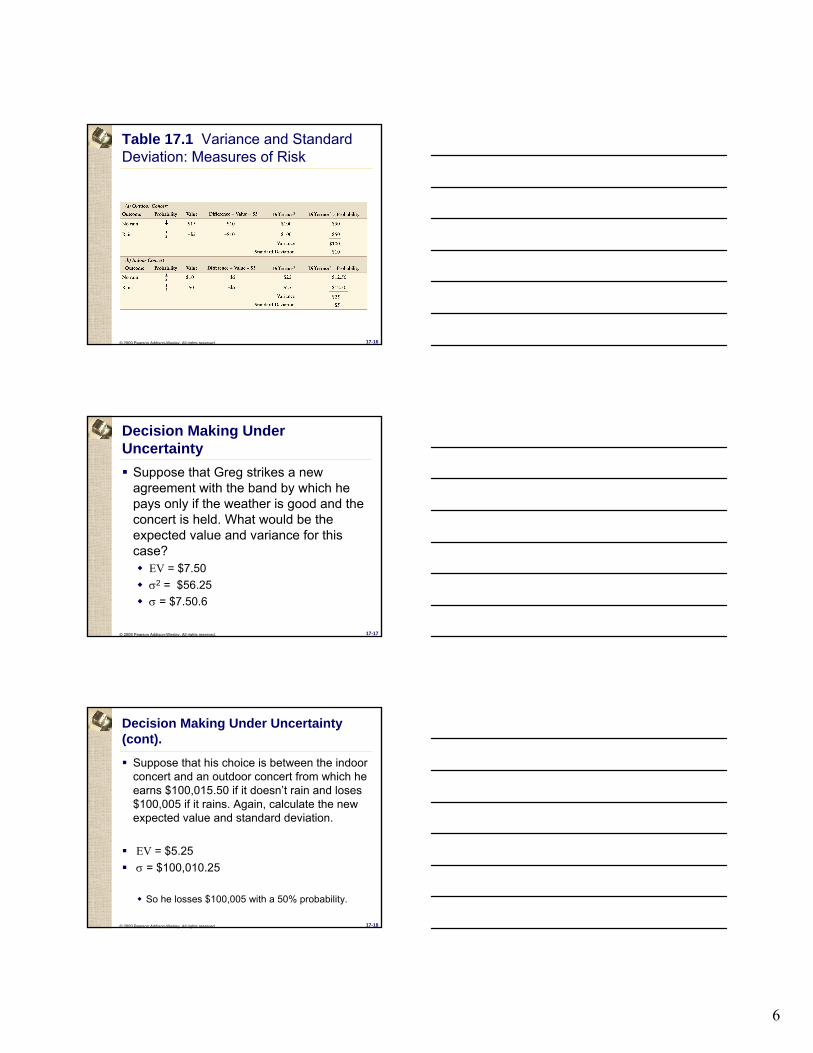
Expected Utility

expected utility (EU) - the probability-weighted average of the utility from each possible outcome.

For example, Gregg’s EU from the outdoor concert is:

( ) ( )

( ) ( )

(norain) Value(no rain) (rain) Value(rain)

1 1$15 $5 ,2 2

= × + ×⎡ ⎤ ⎡ ⎤⎣ ⎦ ⎣ ⎦⎡ ⎤ ⎡ ⎤= × + × −⎢ ⎥ ⎢ ⎥⎣ ⎦ ⎣ ⎦

EU Pr U Pr U

U U


Expected Utility (cont).

fair bet - a wager with an expected value of zero.

Example: you pay a dollar if a flipped coin comes up heads and receive a dollar if it comes up tails. Because you expect to win half the time and lose half the time EV is:

( ) ( )1 1$1 $1 0.2 2⎡ ⎤ ⎡ ⎤= × − + × =⎢ ⎥ ⎢ ⎥⎣ ⎦ ⎣ ⎦



risk averse - unwilling to make a fair betrisk neutral - indifferent about making a fair betrisk preferring - willing to make a fair bet

8


Irma, who is risk averse, makes a choice under uncertainty. She has an initial wealth of $40 and has two options:

nothing and keep the $40.buy a vase.

Her wealth is:$70 if the vase is a Ming and $10 if it is an imitation.

Irma’s subjective probability is 50% that it is a genuine Ming vase.



Figure 17.2 Risk Aversion

Util

ity, U

Wealth, $10 26 40 64 70

a

b

d

e

U(Wealth)U($70) = 140

0.1U($10) + 0.9 U($70) = 133

U($40) = 120

U($10) = 70

0

Risk premium

⎧ ⎪ ⎨ ⎪ ⎩

U($26) = 1050.5U($10) + 0.5 U($70) =

c

f


Risk Aversion

A person whose utility function is concave picks the less risky choice if both

choices have the same expected value.

risk premium - the amount that a risk-averse person would pay to avoid taking a risk

9


Solved Problem 17.2

Suppose that Irma’s subjective probability is 90% that the vase is a Ming. What is her expected wealth if she buys the vase? What is her expected utility? Does she buy the vase?


Risk Neutrality

Someone who is risk neutral has a constant marginal utility of wealth:

Each extra dollar of wealth raises utility by the same amount as the previous dollar.

the utility curve is a straight line in a utility and wealth graph.

a risk-neutral person chooses the option with the highest expected value,

because maximizing expected value maximizes utility.


Risk Preference

An individual with an increasing marginal utility of wealth is risk preferring:

willing to take a fair bet.

10


Avoiding Risk

Just Say NoObtain InformationDiversifyInsure


Correlation and Diversification.

The extent to which diversification reduces risk depends on the degree to which various events are correlated over states of nature.


Correlation and Diversification (cont).

If you know that the first event occurs, you know that the probability that the second event occurs is lower if the events are negatively correlatedand higher if the events are positively correlated.

The outcomes are independent or uncorrelated if knowing whether the first event occurs tells you nothing about the probability that the second event occurs.

11



Diversification can eliminate risk if two events are perfectly negatively correlated.



Suppose that two firms are competing for a government contract and have an equal chance of winning.

Because only one firm can win, the other must lose, so the two events are perfectly negatively correlated.



You can buy a share of stock in either firm for $20.

The stock of the firm that wins the contract will be worth $40, the stock of the loser will be worth $10. If you buy two shares of the same company, your shares are going to be worth either $80 or $20 after the contract is awarded.

12



Their expected value is:$50 = (1/2 x $80) +(1/2 x $20)

And the variance:

However, if you buy one share of each, your two shares will be worth $50 no matter which firm wins, and the variance is zero.

( ) ( )2 21 1$900 $80 $50 $20 $50 .2 2⎡ ⎤ ⎡ ⎤= × − + × −⎢ ⎥ ⎢ ⎥⎣ ⎦ ⎣ ⎦



The more negatively correlated two events are, the more diversification

reduces risk.

Diversification does not reduce risk if two events are perfectly positively

correlated.


Mutual Funds

mutual fund - issued by a company that buys stocks in many other companies.

13


Insure

Because Scott is risk averse, he wants to insure his house, which is worth $80 (thousand).

There is a 25% probability that his house will burn next year. If a fire occurs, the house will be worth only $40.With no insurance, the expected value of his house is:

1 1$40 $80 $70.4 4

⎛ ⎞ ⎛ ⎞× + × =⎜ ⎟ ⎜ ⎟⎝ ⎠ ⎝ ⎠


Insure (cont).

The variance of the value of his house is

( ) ( )2 21 3$40 $70 $80 $70 $300.4 4⎡ ⎤ ⎡ ⎤× − + × − =⎢ ⎥ ⎢ ⎥⎣ ⎦ ⎣ ⎦


Insure (cont).

fair insurance - a bet between an insurer and a policyholder in which the value of the bet to the policyholder is zero.

The insurance company offers to let Scott trade $1 in the good state of nature (no fire) for $3 in the bad state of nature (fire).

This insurance is fair because the expected value of this insurance to Scott is zero:

( )1 3$3 $1 $0.4 4⎡ ⎤ ⎡ ⎤× + × − =⎢ ⎥ ⎢ ⎥⎣ ⎦ ⎣ ⎦

14


Insure (cont).

Because Scott is risk averse, he fully insures by buying enough insurance to eliminate his risk altogether.


Insure (cont).

Scott pays the insurance company $10 in the good state of nature and Receives $30 in the bad state.

In the good state, he has a house worth $80 less the $10 he pays the insurance company, for a net wealth of $70. If the fire occurs, he has a house worth $40 plus a payment from the insurance company of $30, for a net wealth, again, of $70.

Scott’s expected value with fair insurance, $70, is the same as his expected value without insurance. The variance he faces drops from $300 without insurance to $0 with insurance. Scott is better off with insurance because he has the same expected value and faces no risk.


Solved Problem 17.3

The local government assesses a property tax of $4 (thousand) on Scott’s house. If the tax is collected whether or not the house burns, how much fair insurance does Scott buy? If the tax is collected only if the house does not burn, how much fair insurance does Scott buy?

15


Risk-Neutral Investing.

Chris, the owner of the monopoly, is risk neutral.

She maximizes her expected utility by making the investment only if the expected value of the return from the investment is positive.


Figure 17.4 Investment Decision Tree with Risk Aversion


Risk-Averse Investing.

Ken, who is risk averse, faces the same decision as Chris.

Ken invests in the new store if his expected utility from investing is greater than his certain utility from not investing.

16


Figure 17.4 Investment Decision Tree with Risk Aversion (cont’d)


Investing with Uncertainty and Discounting

How does this rule change if the returns are uncertain?

A risk-neutral person chooses to invest if the expected net present value is positive.


Figure 17.5 Investment Decision Tree with Uncertainty and Discounting

17


Investing with Altered Probabilities

Gautam, who is risk neutral, is considering whether to invest in a new store.

After investing, he can increase the probability that demand will be high at the new store by advertising at a cost of $50.If he makes the investment but does not advertise, he has a 40% probability of making $100 and a 60% probability of losing $100.


Figure 17.6 Investment Decision Tree with Advertising


Gambler’s Fallacy.

gambler’s fallacy - arises from the false belief that past events affect current, independent outcomes

18


Certainty Effect.

First, a group of subjects were asked to choose between two options:

Option A. You receive $4,000 with probability 80% and $0 with probability 20%.Option B. You receive $3,000 with certainty.The vast majority, 80%, chose the certain outcome, B.

Then, the subjects were given another set of options:

Option C. You receive $4,000 with probability 20% and $0 with probability 80%.Option D. You receive $3,000 with probability 25% and $0 with probability 75%.

Now, 65% prefer C


Certainty Effect.

Kahneman and Tversky found that over half the respondents violated expected utility theory by choosing B in the first experiment and C in the second one.


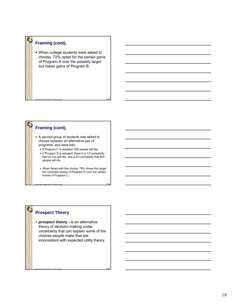
Framing.

The United States expects an unusual disease (e.g., avian flu) to kill 600 people.

The government is considering two alternative programs to combat the disease.The “exact scientific estimates” of the consequences of these programs are:

If Program A is adopted, 200 people will be saved.If Program B is adopted, there is a 1 3 probability that 600 people will be saved and a 2/3 probability that no one will be saved.

19


Framing (cont).

When college students were asked to choose, 72% opted for the certain gains of Program A over the possibly larger but riskier gains of Program B.


Framing (cont).

A second group of students was asked to choose between an alternative pair of programs, and were told:

If Program C is adopted, 400 people will die.If Program D is adopted, there is a 1/3 probability that no one will die, and a 2/3 probability that 600 people will die.

When faced with this choice, 78% chose the larger but uncertain losses of Program D over the certain losses of Program C.


Prospect Theory

prospect theory - is an alternative theory of decision-making under uncertainty that can explain some of the choices people make that are inconsistent with expected utility theory.

20


Additional Chapter Art


Figure 17.3 Risk Neutrality and Risk Preference


Application Gambling

21


Figure 17.7 Prospect Theory Value Function

Chapter Seventeen - wps.aw.comwps.aw.com/wps/media/objects/5495/5627212/ppt/ch17.pdf · Chapter...

Documents

Transcript of Chapter Seventeen - wps.aw.comwps.aw.com/wps/media/objects/5495/5627212/ppt/ch17.pdf · Chapter...