CHAPTER IV - publishing.cdlib.org IV General Distribution of Temperature, Salinity, and Density

CHAPTER IV

General Distribution of Temperature, Salinity, and Density

............... ............... ........... ........................ .........................................

The Heat Budget of the Earth cma Whole

For the earth as a whole, the total amount of heat that is receivedduring one year from the sun at the limit of the atmosphere must exactlybalance the total amount that in the same period is lost by reflectionand by radiation into space. Otherwise, the temperature of the atmos-phere and the oceans would change. The radiation from the hot sun iscalled short-wave radiation, because the wave lengths which reach thelimit of the earth’s atmosphere lie roughly between 0.38 P and 2.5 p,whereas the dark-heat radiation which is emitted by all objects atordinary temperatures is called long-wave radiation, being of wavelengths between 5 P and 20 M. The part of the short-wave radiation thatis re$ected is of no importance to the heat budget of the earth, andtherefore the amount of short-wave radiation that is absorbed by theatmosphere, the oceans, and the land must exactly balance the long-wave radiation into space from the entire system. A small part of theheat that the atmosphere receives is transformed into kinetic energywhich by friction is transformed back again to heat and ultimately lostinto space by radiation. Thus, the transformation of heat to kineticenergy does not lead to any net gain of heat but serves to maintain thecirculations of the atmosphere and the oceans.

As is customary procedure, the amounts of heat will be given ingram calories and not in units of work such as ergs or joules. The con-version factors are: 1 gram calorie = 4.183 X 107ergs = 4.183 joules.

In lower latitudes, heat received by radiation is greater than heatlost by back radiation and reflection, whereas in higher latitudes the gainis less than the loss. Table 24 contains values of heat received andlost by processes of radiation and reflection in different latitudes. Thethird column, containing the differencesbetween the two quantities,showsthat there is an annual net gain of heat in the equatorial regions and a netloss in the polar regions. The mean annual temperatures in differentlatitudes on the earth remain unchanged from one year to another, show-ing that within the atmosphere and the oceans there must be a transportof heat from lower to higher latitudes which exactly equals the difference

98

DISTRIBUTION OF TEMPERATURE, SALINITY, DENSITY 99

between heat received and heat lost by radiation. Multiplying theaverage difference between any two parallels of latitude by the areaof the earth’s surface between these parallelsand summing up, starting attho Equator, gives the total amounts of heat that flow from the Equatortoward the poles in every latitude. Some of these values are given in thefourth column in the table, from which it is seen that they are of the orderof 1016g cal/min, Dividing the numbers by the length of the parallelsgives the amounts shown in the fifth column of the table, which representthe average flow of heat across each centimeter of the parallelsof latitu&These numbers are of the order of 107g cal/cm/min.

The transport of heat from lower to higher latitudes takes place partlyby air currents (winds) and partly by ocean currents. In meteorologicalliterature it is generally assumed that the transport by ocean currents isnegligible (Bjerknes et al, 1932), although the question has not beenthoroughly examined. It can be shown that the assumption is correctwhen dealing with averages for the whole earth, but in some regions thetransport by ocean currents is of considerable importance.

TABLE24HEAT BUDGET OF THE EARTH AS A WHOLE AND HEAT TRANSPORT

FROM LOWER TO HIGHER LATITUDES

Latitude(0)

o . . . . . . . . .lo . . . . . . . . .20. . . . . . . . .30. . . . . . . . .40. . . . . . . . .50. . . . . . . . .60. . . . . . . . .70. ..!..,..80. . . . . . . . .90. . . . . . . . .

Heatreceived

(g cal/cm2/rein)

0.3390.3340.3200.2970.2670.2320.1930.1600.1440.140

Heat lost(g o:l&m’/

0.3000.2990.2940.2830.2720.2580.2450<2310.2200.220

Surplusordeficit

(g e$~)m’/

0.0390.0350.0260.014

-0.005-0.026-0.052-0.071–0.076-0.030

Heat trans-port acroseparallelsof

latitude(10:%;W

0.001.592.943.583.963.342.401.200.320.00

Heat trans-portaorosseverycenti-

meterofparallelsof

latitude(107g cal/cm/min)

0.000.400.781.071,301.321.20 ,0.880.460.00

The amount of heat transported in a north-south direction by a unitvolume of ocean water is equal to c@?)N,where c represents the specificheat, p the density, 8 the temperature of the water, and vii the north-south component of velocity. The total transport through a certainsection of the sea can be found by integration, but for the sake of sim-

100 DISTRIBUTION OF TEMPERATURE, SALINITY, DENSITY

plicity we shall assume that this transport can be written c8pTN, where~ represents the average temperature of the water and pTNrepresentsthe mass of water passing north through the section in unit time. Ifthe section is taken across an ocean, the mass transport to the north,PTN,must equal the mass transport to the south, PTS, but the heattransport may differ because the temperature of the water transported inone direction may be higher or lower than that of the water which istransported in the opposite direction. If these temperatures are desig-nated by #i.? and 8s, the net transport of heat will be c(8 M— r3s)pT,where pT now means the transport to the north and the south. As anexample, we can apply these considerations to the North Atlantic Oceanalong the parallel of 55*N, In the eastern Atlantic about 10 millionm3/sec of warm water flow toward the north, and in the western Atlantican equal volume of cold water is carried south by the Labrador Currentand by the flow of the deep water (p. 684). With 0 M— OS= 5°, c = 1,

=1, and T= 10 X 10sm$/see, we find that the heat transport towardthe north through latitude 55° in the Atlantic Ocean is about 0.3 X1010g cal/min. The total heat transport across the parallel of 55*N isabout 3 X 1016g cal/min; hence in the North Atlantic the fraction carriedby the ocean currents is appreciable,

This example represents an outstanding case of poleward transportof heat by ocean currents. In the Pacific Ocean a transport of com-parable magnitude probably takes place in latitudes 30”N to 40”N,but in the southern oceans the north-south circulation and the cor-responding temperature contrasts between currents flowing toward oraway from the higher latitudes are smaller than those in the northernoceans. A detailed study of the transport of heat by ocean currents hasnot been made, but it seems certain that by far the major transport ofheat is taken care of by the atmosphere.

The Heat Budget of the Oceans

The above consideration applies to the entire system formed by theatmosphere and the oceans, but for the oceans alone we encounter anentirely different picture. On an average, the gain of heat must exactlybalance the loss, but the processes involved are not limited to those ofradiation, as is evident from the list at the bottom of page 101.

These processes will be discussed in detail, but it can already bestated that of the processes of heating only the first one is important,and the heat budget of the oceans as a whole can therefore be written

Q,– Qb– Q~– Qe=O,

where Q. is the heat received,70°S the average amounts (in(1936),

Over all ocean surfaces between 70”N andg cal/cm2/min) are, according to Mosby

101DISTRIBUTION OF TEMPERATURE, SALINITY, DEN!+XTY

Q, = 0.221 Q, = 0.090$ = 0.013

a = 0.118Total 0.221 0.221

If a specific region is considered, it must be taken into account thatheat may be brought into or out of that region by ocean currents orby processes.of mixing, and that during short time intervals a certainamount of heat may be used for changing the temperature of the water.The complete equation for the heat balance of any part of the ocean in agiven time interval is, therefore,

Q.– Qb-Qe– Qa+Qv+Q&=ot

where Qo represents the net amount which by currents or processes ofmixing is brought into or out of the region, and where Q$ represents theamount of heat used locally for changing the temperature of the seaw~ter.

RADIATIONFROMTHE SUN ANDTHE SKY. The short-wave radiationthat reaches the sea surface comes partly directly from the sun andpartly from the sky as refiected or scattered radiation. The amount ofrs,dlation energy which is absorbed per unit volume in the sea dependsupon the amount of energy that reaches the sea surface, the reflectionfrom the sea surface, and the absorption coefficients for total energy.The incoming radiation depends mainly upon the altitude of the sun,the absorption in the atmosphere, and the cloudiness. With a clearsky and a high sun, about 85 per cent of the radiation comes directlyfrom the sun and about 15 per cent from the sky, but with a low sun theproportion from the sky is greater, reachkg about 40 per cent of the totalwith the sun 10 degrees above the horizon.

Processes of Heating of the t%san Procew+es of Cooling of the Ocean

1,

2.

3.

4.

5.

6.

WaterAbsorption of radiation from the 1.

sun and the sky, Q,.Convection of hpat through the 2.

ocean bottom from the interiorof the earth.

Transformation of kinetic energy 3.to heat.

Heating due to chemical proc-esses.

Convection of sensible heat fromthe atmosphere.

Condensation of water vapor.

WaterBack radiation from the sea

surface, Q6.Convection of sensible heat to

the atmosphere, Qfi.

Evaporation, Q..


The incoming energy from the sun is cut down when passing throughthe atmosphere, partly through absorption by water vapor and carbondioxide in the air and partly through scattering against the air moleculesor very fine dust. The total effect of absorption and scattering in theatmosphere depends upon the thickness of the air mass through whichthe sun’s rays pass, as expressed by the equation

Here 1 representsthe energy in g cal/cmZ/min reachkg a surface which isnormal to the sun’s rays; m represents the relative thickness of the airmass and is equal to 1 at a pressure of 760 mm when the sun stands inzenith, equal to 2 when the sun is 30° above the horizon (sin 30° = ~),and so on; S is the solar constant (1.932 g cal/cmz/min); T is the” turbid-ity factor” of the air; and u~ is 0.128 — 0.054 log m.

The sun’s radiation on a horizontalsurface is obtained by multiplica-tion with sin h, where h is the sun’s altitude. To this amount must beadded the diffuse sky radiation in order to obtain the total radiation ona horizontal surface. Instruments are in use for recording the totalradiation and for recording separately the radiation from the sunandfromthe sky.

When the sun is obscured by clouds, the radiation comes from the skyand the clouds and, on an average, can be represented by the formulaQ = Qo(l – 0.071 C), where the cloudiness C is given on the scale O~o 10,and where QOrepresents the total incoming radiation with a clear sky.This formula is applicable, however, only to average conditions. If thesun shines through scattered clouds, the radiation may be greater thanwith a clear sky, owing to the reflection from the clouds, and on a com-pletely overcast dark and rainy day the incoming radiation may be cutdown to less than 10 per cent of that on a clear day. Table 25 containsthe average monthly amounts of incoming radiation, expressed ing cal/cm2/min, which reach a horizontal surface in the indicated localities(computed from Kimball, 1928). The differences between the partsof the oceans in the same latitudes are mainly due to differences incloudiness.

Few direct measurementsof radiation are available from the oceans,and when dealing with the incoming radiation it is necessary to consideraverage values which can be computed from empirical formulae. Mosby(1936) has established such a formula by means of which monthly orannual mean values of the incoming radiation on a horizontal surfacecan be computed if the corresponding average altitude of the sun and theaverage cloudiness are known:

Q = k(l – 0.071C)fi(g cal/cm’/min). ‘

DISTRIBUTION OF TEMPERATURE/ SALININ, DENSITY 103

Ag

z!

%4$3

WM! ==s ,.WW%Niw. . . . . .. ... . . . . b..”

.3’j

3

.“<

..

. . . . . . . .. . . . . . . .. . . . . . . .. . . . . . . .. . . . . . . .. . . . . . . . .. . . . . . . . .. . . . . . . . .. . . . . . . . .. . . .

. .,. . .. . .. . .. . .. ..:

. .. .. .. .. .. .. . .. . . . . .. .. .. . . .. .. .. .

. . .. .. . .tiiiai i+iui rziti

0’s3C@-s

104 DISTRIBUTION OF TEMPERATURE, SALININ, DENSITY

Here i is the average altitude of the sun. The factor k depends upon thetransparency of the atmosphere and appears to vary somewhat withlatitude, being 0.023 at the Equator, 0.024 in lat. 40”, and 0.027 in lat. 70”.Mosby’s formula is not valid at h >60°, but gives correct results if, athigh altitudes of the sun, the true altitude is replaced by a reducedaltitude as follows:

Truealtitude (”).., . . . . . . . . . . . . . . . . . . . . . . . . . . . ...60 65 70 75 80 85 90Reduced altitude (0). . . . . . . . . . . . . . . . . . . . . . . . . ...60 62 64 66 68 69 70

The values computed by meansof this formula agree within a few per centwith those derived by Kimball in an entirely different manner (table 25).

Part of the incoming radiation is lost by reflection from the sea sur-face, the loss depending upon the altitude of the sun. When computingthe loss, the direct radiation from the sun and the scattered radiationfrom the sky must be considered separately. With the sun 90°, 60°,30° and 10° above the horizon, the reflected amounts of the direct solarradiation are, according to Schmidt (1915), 2.0 per cent, 2,1 per cent,6.0 per cent, and 34.8 per cent respectively. For dtiuse radiation fromthe sky and from clouds Schmidt computes a reflection of 17 per cent.Measurements by Powell and Clarke (1936) gave values on clear daysin agreement with the above, but on overcast days when all radiationreaching the sea surface was diffuse, the observed reflection was about8 per cent. If the fractions of the total radiation from the sun andthe sky on a clear day are designated p and q, respectively, andif the corresponding percentages reflected are designated m and n, thepercentage of the total incoming radiation that is reflected on a clearday is r = mp + rig. Thus, on an overcast day, when all incoming

TABLm26PERCENTAGE OF TOTAL INCOMING RADIATION FROM SUN AND SKY

WHICH ON A CLEAR DAY IS REFLECTED FROM A HORIZONTALWATER SURFACE AT DIFFERENT ALTITUDES OF THE SUN

Altitudeof thesun (”) . . . . . . . . . . . . . . . 5 10 20 30 40 50 60 70 80 90Percentagereflected. . . . . . . . . . . . . . . . . .40 25 12 6 4 3 3 3 3 3

radiation is diffuse, r = 8 per cent. Table 26 contains approximatevalues of r at different altitudes of the sun on a clear day.

The values in the table are applicable only if the sea surface is smooth.In the presence of waves the reflection loss at a low sun is somewhatincreased and will be of particular importance in high latitudes. Theamount of radiation which under stated conditions penetrates the seasurface is obtained by~subtractingthe reflection loss~fromthe total incom-ing radiation.

ABSORPTIONOF RADIATIONENERGYIN THE SEA. The radiation thatpenetrates the surface is absorbed in the sea water. The amountsabsorbed within given layers of water can be derived by measuring with


a thermopile the energies which reach different depths or by computingthese energie~ by means of known extinction coefficients. Directmeasurements of energy have been made in Mediterranean waters only(Vercelli, 1937), but extinction coefficients of radiation of different wavelengths have been determined in many areas (p. 85). For computationof the energy that reaches a given depth, it is necessary to know theintensity of the radiation at clifferent wave lengths; that is, the energyspectrum. The reduction in intensity has to be calculated for eachwave length, and the total energy reaching a given depth has to bedetermined from the energy spectrum by means of integration. Thedefinition of the extinction coefficient for total energy corresponds tothe definition of extinction coefficients at given wave lengths (p. 82).

‘3P43~7~9 1.0 1,1 !.2 13 1.4 IS 16 17 15 !9 20 21 22 23 24/IWAVE LENGTH

Fig. 21. Schematicrepresentationof the energy spectrumof tlie radiationfromthe sunand the sky whkh penetratesthe seasurface,and of the energyspeotrain purewater at depths of 0.1, 1, 10, and 100 m, Inset: Percentagesof total energy andof energyin thevisiblepart of the speotrumreachingdit%rentdepths.

The spectrum of the energy that penetrates the sea surface is repre-sented approximately by the upper curve in fig. 21, which also shows theenergy spectra at different depths in pure water, The total energyat any given depth is proportional to the area enclosed between the baselime and the curves showing the energy spectrum. In the inserteddiagram the total energy, expressed as percentage of the energy pene-trating the surface, as well as the corresponding percentages of the energyin the visible part of the spectrum, is plotted against depth. Thefigure shows that pure water is transparent for visible radiation only.

For sea water the percentage of the total energy reaching variousdepths has been computed for the clearest oceanic water, for average


oceanic water, for average coastal water, and for turbid coastal water, us-ing the extinction coefficients shown in fig. 20. The results are presentedin table 27. In the clearest offshore water, 62.3 per cent of the incomingenergy is absorbed in the first meter. The absorption is often increasedin the upper one meter owing to the presence of foam and air bubbles.Thk increased absorption, when dealing with the penetration of light,is referred to as “surface loss.” If this process is disregarded, the valuesclearly demonstrate that the greater amount of energy is absorbed verynear the sea surface and that the amount which penetrates to anyappreciable depth is considerable only when the water is exceptionallyclear. At 10 m, 83.9 per cent has been absorbed in the clearest waterand 99.55 per cent in the turbid coastal water.

Fig. 22. Energy spectraat a depth of 10 m in differenttypes of water. CurvesmarkedO,1, 2, 3, and 4 representenergyspectrain purewater,clearoceanic,averageoceanic, average coastal, and turbid coastal sea water, respectively. Inset: Energyspectra at a depth of 100 m in clear oceanic water and at 10 m in turbid coastalwater.

The absorption of energy is illustrated in fig. 22, which shows theenergy spectra in different types of water at a depth of 10 m. At thisdepth the maximum energy in the clearest water is found in the blue-green portion of the spectrum, whereas in the turbid coastal water themaximum has been displaced toward the, greenish-yellow part. Thisdisplacement is further illustrated by the inserted curve in the upperright-hand corner of the figure, which shows the energy spectra at 100 min the clearest water and at 10 m in the most turbid water.

Extinction coefficients of total energy have. been computed and areentered in table 27. These extinction coefficients are very high in theupper 1 m but decrease rapidly, at greate~depth approaching the mini-mum extinction coefficients characte$stic. of the types of water dealtwith. The smallestvalues given in the table can.be considered valid atgreater depths as well.

DISTRIBUTION OF TEMP~ATURE, SALINITY, DENSITY 107

. .

. .,.. . . . .,.. .,..,,. .. . . .

.. . . .

. .

.. . . .. .., ..


In fig. 23 the curves marked O, 1, 2, 3, and 4 represent the percentageamounts of energy which reach different levels between the surface and10 m, according to the data in table 27. The three curves marked Capri,Trieste, and Venice represent results of measurements in the Mediter-ranean according to Vercelli (1937), and four other curves representobserved values in lakes according to Birge and Juday (1929). Theagreement of the character of the curves indicates that reliable valuesas to the absorption of energy in the sea can be obtained by means of-.computations based on observed extinction coefficients.

tPERCENTAGE OF TOTAL ENCRGY

Is 2 3456 B 10 Is 20 4050 ICC

- 2.

74.

E

r’

i

:

—6

- -e-

Fig. 23. Percentagesof total energy reaching clifferent depths in pure water,clear oceanic, averageoceanic, averagecoastal, and turbid coastal sea water (curvesO, 1, 2, 3, arid 4), c&nputed from ex~inctioncoefficients,and correspondingduectlyto observed valuesin four lakesand at three localitiesin the Mediterranean.

An idea of the heating due to absorption of radiation can be securedby computing the increase of temperature at different depths whichresults from a penetration of 1000 g cal/cm2 through the surface. Theresultsare shown in table 28, which serves to emphasize that the greaterpart of the energy is absorbed near the surface, particularly in turbidwater. If no other processes took place, the temperature between thesurface and 1 m would increase in the clearest water by 6,24°, and inthe most turbid water by 7.72°. Between 20 and 21 m the correspondingvalues would be 0.04° and 0.0003°.

The temperature changes recorded in table 28 show no similarityto those actually occurring in the open oceans, where processes of mixingentirely mask the direct effect of absorption, but in some small, land-


locked bodies of water the temperature changes at subsurface depths maybe governed mainly by absorption of short-wave radiation, Suchprocesses may be observed in the oyster basins on the west coast ofNorway, the temperature characteristics of which were described byHelland-Hansen and studied in detail by Gaarder and Spiirck (1932).These basins are in communication with the open sea through narrowand shallow openings, but during winter storms a complete exchange ofwater often takes place between the basins and the outside. In theensuing spring, after rains, which cause considerable run-off, the surfacelayer in the basins will be replaced by fresh or brackish water spreadingover the sea water in the deeper portion of the basinsand forming a cover

Tmm 28

TEMPERATURE INCREASE IN “C AT DIFFERENT DEPTH INTERVAJJSAND IN DIFFERENT TYPES OF WATER, CORRESPONDING TO AN

ABSORPTION OF 1000 G CAL/CM~

OceanicwaterInterval of depth

(m)Clearest

I

6.240.610

.236

.104

.040

.0096

.0016

Average

6.480.720

.282

.096

.030

.0024

.0411

Coastalwater

Average

7.320.970

.164

.030

.0016

.0534

Turbid

7.720.960

.120

.0140

.0003

.0715

that prevents further exchange between the deeper water and the outsidesea. Owing to the difference in salinity the density of the deeper waterwill be muoh higher than the density of the surface layer. Duringsummerthe incoming radiation will be absorbed both in the fresh water ontop and in the underlying sea water, and the temperature will rise withinboth layers. Withh the top layer the ordinary convection currentsdevelop, and the temperature is controlled mainly by the air temperature,but owing to the greater ,salinity of the lower layer the temperature ofthe deeper water can rise to high values without leading to unstablestratification, and the effect of absorption becomes apparent, because noother processes are of importance.

Fig. 24 shows the vertical distribution of temperature on June 30 andJuly 15 in a basin that was examined by Gaarder and Sp5rck. Thedays in the period between the stated dates were clear and no rain fell.According to Kimball (1928) the diurnal amount of incoming short-waveradiation was about 740 g cal/cm2/day, or about 11,100 g cal/cm2 for


the entire period. If 6 per cent is subtracted for reflection, the amountentering the water would be about 10,400 g cal/cm2. The temperaturecurves show that of thk amount 1630 g cal/cm2, or 15.5 per cent, wasabsorbed below a depth of 1 m, and thus 84.5 per cent was absorbedbetween the surface and 1 m. The latter amount was lost by backradiation, heat conduction to the atmosphere, and evaporation, and atpresent need not be further considered. It is of interest, however, topoint out that the great absorption in the upper meter indicates thatthe turbidity of the water in the basin was greater than that of ordinarycoastal waters (table 27, fig. 23) and approached that of turbid lakes.The heating between 1 and 2 m also indicates water of great turbidity,

because, of the total amount ofIs” [ Z@ *

~. S<@% ‘“ ‘“’ a“ c 1630 g cal/cm2 reaching 1 m, 630---------------------------------:

?

./:g cal/cm2 were absorbed in that

~;x

“?layer, the corresponding extinction

3:

/

coefficient being 0.488 (cf. table 27).JUNE201927 JULY 15,1927 Thk result agrees roughly with

‘ 4’/ ~ Gaarder and Splirck’s statementthat aSecchl dkc nearly disappeared

Fig. 24. Vertical distribution of at a depth of only 2 m: Conditionstemperaturein a Norwegianoyster basinon June 30 and July 15, 1927. in this case were unusually clear

cut, but even in such basins theeffect of absorption is often obscured by processes of heat conduction.

CONDUCZWONOF HEAT THROUGHTHE OCEAN BOTTOM. It has beenestimated that the flow of heat through the bottom of the sea amounts tobetween 50 and 80 g cal/cmz/year (Helland-Hansen, 1930). Thisamount represents less than one ten-thousandth part of the radiationreceived at the surface and can generally be neglected when dealing withthe heat budget of the oceans. In a few basins, where the deep water isnearly stagnant and where no conduction of heat takes place from aboveor from the sides, the amount of heat conducted through the bottom mayconceivably play a part in determining the dktribution of temperature,but so far no such case is known with certainty (p. 739).

TRANSFORMATIONOF KINETIC ENERGY INTO HEAT. The kineticenergy transmitted to the sea by the stress of the wind on the surface andby part of the tidal energy is dissipated by friction and transformed intoheat. The energy transmitted by the wind can be estimated at aboutone ten-thousandth part of the radiation received at the surface and canbe neglected. In shallow coastal waters with strong tidal currents thedksipation of tidal energy is so great, however, that it may become ofsome local importance. Thusj in the Irish Channel, according to Taylor(1919), the dissipation amounts to about 0.002 g cal/cm2/min, or 1050g cal/cm2/year. The average depth can be taken as about 50 m, or5000 cm, and, if the same water remained in the Irish Channel a full year,


the increase in temperature would be about 0,2°C, on an average. Suchan effect, howeverj has not been e$t%blished,and, as it can be expected inshallow coastal waters only, it is of no significance to the general heatbudget of the oceans. A possible case of heating due to dissipation oftidal energy or to conduction of heat through tho ocean bottom has beendiscussed by Sverdrup (1929).

Heating due to chemical processes can be completely dieregarded.The convection of sensible heat and the condensation of water vapor

will be dealt with in the discussion concerning the exchange of heat andwater with the atmosphere,

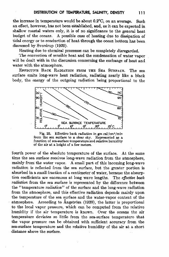
EFFECTIVE BACK RADIATION FROM T~EI SEA SURFACE. The seasurface emits long-wave heat radiation, radiating nearly like a blackbody, the energy of the outgoing radiation being proportional to the

SEA SUWA$E TEMPERATURE

Fig. 25. Effective back radiationin gm callcm%iminfrom the sea surface to a clear sky. Representedas afunction of sea-surfacetemperatureandrelativehumidityof the air at a heightof a few meters.

‘fourth power of the absolute temperature of the surface. At the sametime the sea surface receives long-wave radiation from the atmosphere,mainly from the water vapor. A small part of this incoming long-waveradiation is reflected from the sea surface, but the greater portion isabsorbed in a small fraction of a centimeter of water, because the absorp-tion coefficients are enormous at long wave lengths. The e~ectivebacknzdiation from the sea surface is represented by the clifference betweenthe “temperature radiation” of the surface and the long-wave radiationfrom the atmosphere, and this effective radi@ion depends mainly uponthe temperature of the sea surface and the water-vapor content of theatmosphere. According to Angstrom (1920), the latter is proportionalto the local vapor pressure, which can be computed from the relativehumidity if the air temperature is known. Over the oceans the airtemperature deviates so little from the sea-surface temperature thatthe vapor pressure can be obtained with suilicient accuracy from thesea-surface temperature and the relative humidity of the air at a shortdistance above the surface.

1?2 DISTRIBUTION OF TEMPERATURE, SALINITY, DENSITY

&@trom (1920) has published a table that summarizes results ofobservations of effective radiation against a clear sky from a black bodyof clifferent temperatures and at clifferent vapor pressures. Fig. 25 hasbeen prepared by means of this table, taking into account the smalldifference between the radiation of a black body and that of a watersurface. The figure shows the effective radiation as a function of sea-surface temperature and of relative humidities between 100 per cent and70 per cent, but the values that can be read off from the graph may be10 per cent in error, owing to the scanty information upon which thecurves are based. It brings out the interesting fact, however, that,owing to the increased radiation from the atmosphere at higher tempera-tures (higher vapor pressures), the effective back radiation decreasesslowly with increasing temperature. At a temperature of O“C and arelative humidity of 80 per cent, the effective back radiation is 0.188 gcal/cmz/min, and at a temperature of 25° and the same relative humidityit is 0.167 g cal/cm2/min. At a given temperature the effective radiationdecreases with increasing humidity, owing to the increased back radiationfrom the atmosphere. Thus, at a surface temperature of 15° the effectiveradiation is about 0.180 g cal/cm2/min at a relative humidity of 70 percent, and about 0.163 g cal/cm2/min at a relative humidity of 100 percent.

The values of the effective back radiation at higher. temperatures,as obtained by extrapolation of ~ngstrom’s data (fig. 25) are greaterthan those computed from Brunt’s empirical formula,

Q, = Q’(1 – 0.44 – 0.08 ~i),

where Q’ is the radiation of a black body having the temperature ofthe sea surface and e is the vapor pressure of the air in millibars.However, in this formula the numerical values of the coefficients areuncertain and are applicable only within a range of e between 4 and18 mb.

The diurnal and annual variations of the sea-surface temperaturesand of the relative humidity of the air over the oceans are small, and theeffective back radiation at a clear sky is therefore nearly independentof the time of the day and of the season of the year, in contrast to theincoming short-wave radiation from the sun and the sky, which is sub-jected to very large diurnal and seasonal variations.

In the presence of clouds the effective back radiation is cut downbecause the radiation from the atmosphere is increased. The empiricalrelation can be written

Q = Qo(l – 0.083C),

where QOis the back radiation at a clear sky and where C’ is the cloudinesson the scale 1 to 10. A diurnal or annual variation in the cloudiness will


lead to a corresponding variation in the effective back radiation. Onan average, the diurnal variation of cloudiness over the oceans is verysmall and can be neglected, but the annual variation is in some regionsconsiderable. The above equation is applicable to average conditionsonly, because the reduction of the effective back radiation due to cloudsdepends upon the altitude and the density of the clouds. Thus, if thesky is completely covered by cirrus, alto-stratus, or strato-cumulusclouds, the effective radiation is about 0.75Q0, 0.4Q0, and O.lQo,respectively.

The annual incoming short-wave radiation from the sun and the skyis greater in all latitudes than the outgoing effective back radiation.According to Mosby (1936) the average annual surplus of incomingradiation between latitudes O and 10*N is about 0.170 g cal/cm2/min,and between 60° and 70°N about 0.040 g cal/cm2/min. The surplus ofradiation must be given off to the atmosphere, and the exchange of heatand water vapor with the atmosphere is therefore equally as importantas the processes of radiation in regulating the ocean temperatures andsalinities.

The characteristics of the oceans in respect to radiation are veryfavorable to man. The water surface reflects only a small fraction ofthe incoming radiation, and the greater part of the radiation energy isabsorbed in the water, distributed by processes of mixing over a layer ofconsiderable thickness, and given off to the atmosphere during periodswhen the air is colder than the sea surface. The oceans therefore exercisea thermostatic control on climate. Conditions are completely changed,however, if the temperature of the sea surface decreases to the freezingpoint so that further loss of heat from the sea leads to formation of ice,because, when water passes this critical temperature, its thermostaticcharacteristics are altered in a very unfavorable direction, Sea ice,which soon attains a gray-white appearance owing to enclosed air bubbles,reflects 50 per cent or more of the incoming radiation, and if it is coveredby rime or snow the reflection loss increases to 65 per cent, or even to80 per cent from fresh, dry snow. The snow surface, on the otherhand, radiates nearly like a black body, and consequently the heatbudget related to processes of radiation, instead of rendering a surplusas it does over the open ocean, shows a deficit until the temperatureof the ice surface has been lowered so much that the decreased loss byeffective back radiation balances the small fraction of the incoming ‘radiation that is absorbed. The immediate result of freezing is thereforea general lowering of the surface temperature of the ice and a rapidincrease of the thickness of the ice. The air that comes in contactwith the ice is cooled, and, as this cold air spreads, more ice is formed.Thus, a small lowering of the temperature of the water in high latitudesfollowed by freezing may lead to a rapid drop of the air temperature and


a rapid increase of the ice-covered area. On the other hand, a smallincrease of the temperature of air flowing in over an ice-covered sea maylead to melting of the ice at the outskhts and, once started, the meltingmay progress rapidly. In agreement with this reasoning it has beenfound that the extent of ice-covered areasin the Barents Sea is a sensitiveindicator of small changes in’ the atmospheric circulation and in theamount of warm water carried into the region by currents (p. 662), Ithas also been computed that, if the average air temperature in middleand higher latitudes were raised a few degrees, the Polar Sea would soonbecome an ice-free ocean.

EXCHANGEOFHEATBETWEENTHEATMOSPHEREANDTHESEA. Theamount of heat that in unit time is carried away from the sea surfacethrough a unit area is equal to

—CPA()g%,where CP is the specific heat of the air, A is the eddy conductivity,– d&/dz is the temperature gradient of the air (the lapse rate), whichis positive when the temperature decreases with height, and 7 is theadiabatic lapse rate. Very near the sea surface, 7 can be neglected assmall compared to dO/ciz. The term CPAenters instead of the coeffi-cient of heat conductivity of the air as determined in the laboratorybecause the air is nearly always in turbulent motion (p. 92). Thestate of turbulence varies, however, with the distance from the seasurface, because at the surface itself the eddy motion must be greatlyreduced. As a consequence, under steady conditions, when the sameamount of heat passes upward through every cross section of a verticalcolumn, the temperature changes rapidly with height near the sea sur-face and more slowly at greater distance. The product –cPAdOJdzremains constant, and, as. cPA increases rapidly with height, - d8~/dzmust decrease.

Detailed and accurate temperature measurements in the lowestmeters of air over the ocean have not yet been made, because the hull andmasts of a vessel disturb the normal distribution of temperature to suchan extent that values observed at different levels on board a vessel arenot representativeof the undisturbed conditions. The few measurementsthat have been attempted indicate, however, that the generaldistributionas outlined above is encountered.

The sea surface must be warmer than the air at a small distanceabove the surface if heat is to be conducted from the seato the air. Whensuch conditions prevail, the air is heated from below, the stratification ofthe air becomes unstable, and the turbulence of the air becomes intense(p. 92). If the sea surface is very much warmer than the air, as may be


the case when cold continental sir %~wsout over the sea in winter, theheating from below may be so intense that rapid convection currentsdevelop, leadlng to such violent atmospheric disturbances as thunder-storms. It is not intended hereto enter upon the meteorological aspectsof the heat exchange, but the point which is emphasized is that anappreciable conduction of heat from the sea to the atmosphere takesplace only when the sea surface is warmer than the air. One mightassume that, vice versa, an appreciable amount of heat would be con-ducted to the sea surface when warmer air flows over a cold sea, but thisis not the case, because under such conditions the air is cooled from below,the stratification of the air becomes stable, and the turbulence (andconsequently the eddy conductivity of the air) is greatly reduced.

It has been found (p. 128) that on an average the sea surface isslightly warmer than the overlying air and therefore loses heat by con-duction. So far, no detailed studies have been made, but ~ngstromhas estimated that only about 10 per cent of the total heat surplus isgiven off to the atmosphere by conduction and that 90 per cent is usedfor evaporation. Other estimatesindicate that these figuresare approxi-mately correct (p. 117). Thus, evaporation is of much greater impor-tance to the heat balance of the oceans than is the transfer of sensibleheat. Evaporation will therefore be dealt with in greater detail.

Evaporation from the Sea

THE PROCESSOF EVAPORATION. The vapor tension at a flat surfaceof pure water depends on the temperature of the water. The salinitydecreases the tension slightly, the empirical relation between vaportension and salinity being (p. 66)

ef = t?d(l – 0.000537 s),

where e, is the vapor tension over sea water, e,iis $he vapor tension over.distilled water of the same temperature, and S is the salinity in parts permine. In the open ocean the relation is ‘approximately e. = 0.98ed.Table 29 contains the vapor tension in millibars over water of salinity35.00 ‘/00 and at the stated temperatures.

Air in which the vapor tension ia less than that over water of thesame temperature is undm-saturatedwith moisture, and air in which thevapor tension exactly equals that over a water surface of the sametemperature is saturated with moisture. In absolutely pure air thevapor pressure can be above the saturation value, but generally the aircontains “nuclei” on which the vapor is condensed when the vaportension reaches the value corresponding to that over water of the sametemperature. Under these conditions the vapor tension in the aircmmot be further increased, and in meteorology one therefore uses the’


term” maximum vapor tension” at a given temperature. The maximumvapor tension at which condensation takes place can be reached either byadding water vapor to air of a given temperature or by decreasingthe temperature of air of a given moisture content. In the latter casecondensation begins at the temperature that is called the “dew point. ”

TABLE29MAXIMUM VAPOR TENSION IN MILLIBARS OVER WATER OF

SALINITY 35 0/00

Temperature(“c)

–2 . . . . . . . . . . . . . . . . . . . . . . .-1..., . . . . . . . . . . . . . . . . . . .

0 . . . . . . . . . . . . . . . . . . . . . . .1. . . . . . . . . . . . . . . . . . . . . . .2. . . . . . . . . . . . . . . . . . . . . .

3. . . . . . . . . . . . . . . . . . . . .4!. . . . . . . . . . . . . . . . . . . . . .5. . . . . . . . . . . . . . . . . . . . . . .6. . . . . . . . . . . . . . . . . . . . . . .7. . . . . . . . . . . . . . . . . . . . . . .

8. . . . . . . . . . . . . . . . . . . . . . .9. . . . . . . . . . . . . . . . . . . . . . .

10. . . . . . . . . . . . . . . . . . . . . . .11. . . . . . . . . . . . . . . . . . . . . . .12..., . . . . . . . . . . . . . . . . . . .

13. . . . . . . . . . . . . . . . . . . . . . .14. . . . . . . . . . . . . . . . . . . . . . .15. . . . . . . . . . . . . . . . . . . . . . .16. . . . . . . . . . . . . . . . . . . . . . .17. . . . . . . . . . . . . . . . . . . . . . .

vaporpressure

(rob)

5.195.575.996.446.92

7.437.988.569.179.83

10.5211.2612.0512.8813.76

14.7015.6916.7417.8519.02

Temperature(“c)

Vaporpressure

(rob)

20.2621.5722.9624.4225.96

27.5929.3031.1233.0135.02

37.1339.3341.6844.1346.71

In dkcussing the process of evaporation it is more rational to con-sider not the vapor pressurebut the specific humidity, f—-that is, the massof water vapor per unit mass of air. The amount of water vapor, 3’,which per second is transported upward through a surface of crosssection 1 cmz is, then, – Adf/dz, where A is the eddy conductivity and–dj/dz is the vertical gradient of the specific humidity, which is positivewhen the specific humidity decreases with height. If the vapor pressure,e, is introduced, the equation becomes approximately

DISTRIBUTION OF TEMPERATURE, SALINITY, DENSITY, 117

wherep is the atmospheric pressure. The heat needed for evaporation atthe surface is

_L&A 0.621 deQ,= —

p w

where L~ is the heat of vaporization at the temperature of the surface,O (p. 62).

The ratio between the amounts of heat given off to the atmosphere assensible heat (p. 114) and used for evaporation is

The last expression is obtained by introducing CP= 0.240 and L = 585.Thus, the ratio R depends mainly upon the ratio between the temperatureand humidity gradients in the air at a short distance from the sea surface.These gradients are difficult to measure but can be replaced approxi-mately by the difference in temperature and vapor pressure at the seasurface and the corresponding values in the air at a height of a few meters:

p 7% – t?..R=0“661000 e. – e.

This ratio was derived in a different mannerby Bowen (1926), and is oftenreferred to as the ‘‘ Bowen ratio.”

Values of the ratio R can be computed from climakological chartsof the oceans, but a comprehensive study has not been made. Calcula-tions based on data contained in the Atlas of Climatic Charts of the Oceans,published by the U. S. Weather Bureau (1938), show that the ratiovaries from one part of the ocean to the other. As a rule, the ratio issmall in low latitudes, where it remains nearly constant throughout theyear, but is greater in middle latitudes, where it reaches values up to0.5 in winter and in some areas drops to –0.2 in summer. A negativevalue indicates that heat is conducted from the atmosphere to the sea.On an average, the value for all oceans appears to lie at about 0.1, mean-ing that about 10 per cent of the heat surplus that the oceans receive byradiation processesis given off as sensibleheat, whereasabout 90 per centis used for evaporation (p. 115).

There are certain points regarding the character of the evaporationwhich need to be emphasized. If the water is warmer than the air, thevapor pressure at the sea surface remains greater than that in the air,and evaporation can always take place and will be greatly facilitatedin these circumstances because the turbulence of the air will be fullydeveloped owing to the unstable stratification of the very lowest layers(p. 92). It must therefore be expected that the greatest evaporationoccurs when cold air flows over warm water. If the air is much colder


than the water, the air may become saturated with water vapor, and fogor mist may form over the water surfaces. Such fog is common in thefall over ponds and small lakes during calm, clear nights. When a windblows, the moisture will be carried upward, but streaks and columns offog. are often visible over lakes or rivers and are commonly described as‘fsmoke.” The process can occasionally be observed near the coast,but not over the open ocean, because the necessary great temperaturedifferences are rapidly eliminated as the distance from the coast increases.

When the sea surface is colder than the air, evaporation can takeplace only if the air is not saturated with water vapor. In thk caseturbulence is reduced and evaporation must stop when the vapor content

Fig. 26. .Le@ The difference,air minus sea-surfacetemperature,and the prevailingwind-directionover theGrand Banks of Newfoundland in March, April, andMay. It@t: Percentagefrequency of fog in the samemonths.

of the lowest layer of the atmosphere has reached such a value that thevapor pressure equals that at the sea surface. If warm, moist air passesover a colder sea surface, the direction of transport will be reversed andcondensation will take place on the sea surface in such a way that heatis brought to the surface and not carried away from it. Owing to thefact that this process can take place only when the air is warmer thanthe sea and that then turbulence is greatly reduced, one can expect thatcondensation of water vapor on the sea will not be of great importance,but it should be borne in mind that this process can and does take placewhen conditions are right. In these circumstances, contact with thesea and conduction lower the air temperature to the dew point for aconsiderable distance above the sea surface. Condensation takes placein the air and fog is formed, ‘ ‘advection” fog that is commonly encoun-tered over the sea. The relation between the frequency of fog or mistand the difference between sea-surface and air temperatures are wellillustrated by charts in the Atlas of Clirrzatic Charts of the Oceans (1938).As an example, fig. 26 shows the frequency of fog, the difference betweenair and sea-surface temperature, and the prevailing wind direction overthe Grand Banks of Newfoundland in March, April, and May. It canbe concluded that in spring, when the water is colder than the air, no


evaporation takes place in this region, but in the fall and winter, whenthe water is warmer, evaporation must be great.

In middle and higher latitudes the sea surface in winter is mostly “warmer than the air, and hence one must expect the evaporation thento be at its maximum. This conclusion appears contrary to commonexperience that evaporation from heated water is greater than thatfrom cold water, but the contradiction is only apparent, because greatestevaporation always occurs when a water surface is warmer than the airabove it, which is exactly what happens in winter.

OBSERVATIONSANDCOMPUTATIONSOFEVAPORATION.Presentknowl-edge of the amount of evaporation from the different parts of the oceansis derived partly from observations and partly from computations basedon consideration of the heat balance.

Observations have been made by means of pans on board ship, butsuch observations give values of the evaporation from the sea surfacethat are too high, partly because the wind velocity is higher at the levelof the pan than at the sea surface, and partly because the differencebetween vapor pressure in the air and that of the evaporating surface’isgreater at the pan than at the sea surface. Analyzing the decrease ofthe wind velocity and the increase of the vapor pressure between theaverage level of pans used on shipboard and a level a few centimetersabove the sea surface, Wiist (1930) arrived at the conclusion that themeasured values had to be multiplied by 0.53 in order to represent theevaporation from the sea surface.

In computing the evaporation on the basis of the heat balance, onehas to begin with the equation (p. 101)

Introducing the ratio R = Qb/~~, and converting the evaporation, E,.into centimeters by dividing Q. by the latent heat of vaporization, L,oae obtains

~=Q8 –Qb+Q. +Q~. ,L(I + R)

[n thk form the equation representing the heat balance has found wideapplication for computation of evaporation. The result gives theevaporation in centimeters during the time intervals to which the. valuesQ,, and so on, apply, provided these are expressed in gram calories.

A second method for computing the evaporation from the oceans hmbeen suggested by Sverdrup (1937), who, on the basis of results in fluidmechanics as to the turbulence of the air over a rough surface, establisheda formula for the evaporation, using in part constants that had beendetermined by laboratory experiments and in part constants that wereobtained from the character of the variation of vapor prewure with


increasing height above the sea surface. Similar but more complicatedformulae have been derived by Millar (1937) and by Montgomery (1940).

The exact formulae are not well suited for numerical computation,but at wind velocities between 4 and 12 m/see, the mean annual evapora-tion in centimeters can be found approximately from the simple relation

E = 3.7(?W - ?Jti,

where i& represents the average vapor pressure in millibars at the seasurface as derived from the temperature and salinity of the sea, &represents the average vapor pressurein the air at a height of 6 m abovethe sea surface, and ti is the average wind velocity in meters per secondat the same height.

AVERAGEANNUALEVAPORATIONFROMTHEOCEANS. On the basis ofpan measurementsconducted in different parts of the ocean, Wiist (1936)found that the average evaporation from all oceans amounts to 93 cm/year, and he considers this value correct within 10 to 15 per i?ent. W.Schmidt (1915) computed the evaporation by means of the precedingequation for E, in which the terms Q~and Qecan be omitted in consider-ing the oceans as a whole, Schmidt introduced high values of R, andon the basis of the available data as to incoming radiation and backradiation he found a total evaporation of 76 cm/year. A revision basedon more recent measurements of radiation (Mosby, 1936) and use ofR = 0.1 resulted in a value of 106 cm/year. The latter value representsan upper limit, and may be 10 to 15 per cent too high, whence it appearsthat Wtist’s result is nearly correct.

It is of interest in this connection to give some figures regarding tlierelation between evaporation and precipitation over the oceans, theland areas, and the whole earth (according to Wust, 1936). The totalevaporation from the oceans amounts to 334,000 km8/year, of which297,000 km$ returns to the sea in the form of precipitation, and thedifference, 37,OOOkms, must be supplied by run-off, since the salinityof the oceans remains unchanged. The total amount of precipitationfalling on the land is 99,,000kma,of which amount a little over one third,37,000 km8,is supplied by evaporation from the oceans and 62,000 kms issupplied by evaporation from inland water areas or directly from themoist soil. For the sake of comparison it may be mentioned that thecapacity of Lake Mead, above Boulder Dam, is 45 kms.

EVAPORATIONIN DIFFERENT LATITUDES AND LONGITUDES. Frompan observations at sea, Wust has derived average values of the evapora-tion from the different oceans in different latitudes (table 30, p. 123).By means of the energy equation one can compute similar annual val-ues, assuming that the net transport of heat by ocean currents can beneglected. Such a computation has been carried out for the Atlantic

Distribution OF TEMPERATURE, SALINITY, DENSITY 121

Ocean, making use of Kimball’s data (1928) as to the incoming radiationand the observed temperatures and humidities for determining effeotiveback radiation. In fig. 27 are shown Wust’s values of the annualevaporation between latitudes 50°N and 50°S in the Atlantic Oceanand the corresponding values as derived from the energy equation. Theagreement is very satisfactory. The low evaporation in the equatorialregions that both curves show can be ascribed to the higher relativehumidities and the lower wind velocities of that area, if one considersthe processes of evaporation, or it can be ascribed to the effect of theprevailing cloudiness if one considers the energy relations. The great

t , I

~

.1503CM.~

~

“50$

LAT;UDE4ffN 3@ @ Iff Ig 2P C@ sq

Fig. 27. Annual evaporation from the AtlanticOcean between latitudes 50”N and 50°S. Thin curvebased on observations (Wtist, 1936) and heavy ourve oncomputations,using the energy equation.

evaporation in the areas of subtropical anticyelones appears clearly,but in the Southern Hemisphere the observations give the highest valuesof the evaporation nearer to the Equator than do the computations.The discrepancy may be due to the fact that in the course of a year thesubtropical anticyclone changes its distance from the Equator andthat the observations have not been distributed evenly over the year.The energy equation has also been used by McEwen (1938) for computingvalues of evaporation over the eastern Pacific ocean between latitudes20°N and 50”N. His figures agree with those obtained by Wust forthe same latitudes.

It appears that the average annual values of the evaporation indifferent latitudes are well established, but the evaporation also variesfrom the eaeternto the western parts of the oceans and with the seasons.These variations are of great importance to the circulation of the atmos-phere, because the supply of water vapor that later on condenses andgives off its latent heat representsa large portion of the supply of energy.So far, none of the details are known, but it is possible that approximatevalues of the evaporation from different parts of the ocean and in cliffwentseasons can be found by means of the method proposed by Sverdrup(1937) and used by Jacobs (1942).


ANNUAL VARIATIONOF EVAPORATION. The character of the annualvariation of evaporation can be examined by means of the energy equa-tion (Sverdrup, 1940):

Q. = Qe(l+R) =Qg– Q,+ Qo+Qo.

The quantity QOcan be computed if the annual variation of temperaturedue to processes of heating and cooling is known at all depths where suchannual variations occur. The annual variation of temperature at thesurface has been examined, but only few data are available from subsur-face depths, the most reliable being those which have been compiled byHelland-Hansen (1930) from an area in the eastern North Atlanticwith its center in 47”N and 12”W (p. 132). The radiation income in thatarea can be obtained from Kimball’s data (1928), the back radiation canbe found by means of the diagram in fig. 25, and the transport by cur-

,=----+ ~ }0 / / ‘\ \ /A\/ / ..-. - .- Oi

IMIFEBIMRIMIMAYIWNIJWIAWI sqoc TINwoi El@\ 2 4 q 6 “~-’=’””~ p @.zp3&

.4 BFig, 28. (A) Annual variation in the total amount of heat, ~~,given off to the

atmospherein an area of the North Atlantic (about 47°N, 12”W). (B) Correspond-ing diurnal variationnear the Equator in the Atlantic Ocean. (For explanationofsymbols, see text.)

rents, Q., can be neglected. In fig. 28A are represented the annualvariation of the net surplus of radiation, Q,, the annual variation of theamount of heat used for changing the temperature of the water, Qo,and the difference between these two amounts, Qa, which representsthe total amount of heat given off to the atmosphere. The greater partof the last amount is used for evaporation, and the curve marked Q.represents,therefore, approximately the annual variation of the evapora-tion, which shows a maximum in the fall and early winter, a secondaryminimum in February, followed by a secondary maximum in March,and a low minimum in summeri In June and July no evaporation takesplace. The total evaporation during the year is about 80 cm.

This example illustrates a method of approach that may be applied,but so far the necessary data for a more complete study are lacking.The result that the evaporation is at a minimum in summer and at a


&o


maximum in fall and early winter is in agreement with the conclusionsthat were drawn when discussing the process of evaporation in general.

DIURNALVARIATIONOF EVAPORATION.The diurnal variation ofevaporation can be examined in a similarmanner, but at the present timesuitable data are available only at four Meteor stations near the Equatorin the Atlantic Ocean (Defant, 1932; Kuhlbrodt and Reger, 1938), Infig. 28B the curves marked Q, and Q~correspond to the similar curves infig. 28A, and the difference between these, Q., shows the amount of heatlost during twenty-four hours, which is approximately proportional tothe evaporation. The diurnal variation of evaporation in the Tropicsappears to have considerable similarity to the annual variation in middlelatitudes, and is characterized by a double period with maxima in thelate forenoon and the early part of the night and minima at sunrise andin the early afternoon hours, It is possible that the afternoon minimumappears exaggerated, owing to uncertainties as to the absolute values ofQ, and Q~. The total diurnal evaporation was 0.5 cm, but the sky wasnearly clear on the four days that were examined and the average diurnalvalue is therefore smaller. The double diurnal period of evaporationappears to be characteristic of the Tropics, but in middle latitudes asingle period with maximum values during the night probably dominates.

Salinity and Temperature of the Surface Layer

THE SURFACE SALINITY. In all oceans the surface salinity varieswith latitude in a similar manner. It is at a minimum near the Equator,teaches a maximum in about latitudes 20°iN and 20”S, and again decreasestoward high latitudes.

1 , I t , , { ,6g

-35.s g !50.%g ~CM

z gi

.35.0$ ~o.

w ~

~z

-34.5$ iii-w10 .

g

34,0 LAT$UDE %

+“ N 3P” 20” 10” 10° .2@ 30” 40” s~

A

V..

35.5 .

%. :.

%z

35,0; “ “

u.

~“34.5~ “

a

.34.0 . EVA!+ - PRECIR

-s0 o +50 CM

E

Fig. 29. (A) Averagevalues for all oceans of surfaoesalinityand the difference,evaporationminusprecipitation,plotted againstlatitude. (B) “Correspondingvaluesof surfacesalinity and the difference,evaporationminusprecipitation,plotted againsteach other (accordingto Wiist, 1936),

Table 30 contains average values of the surface salinity, the evapora-tion, the precipitation, and the difference between the last quantitiesfor the three major oceans and for all combined, according to Wust (1936).

DISTRIBUTtON OF TEMPERATURE, SALINITY, DENSITY 125

On the basis of these values, Wtist has shown that for each ocean thedeviation of the surface salinity from a standard value is directly propor-tional to the difference between evaporation, E, and precipitation,P. In fig. 29A are plotted the surface salinities for all oceans and thedifference, E - P, in centimeters per year, as functions of latitude; thecorresponding values of salinity and the difference, .?3— P, are plotted .against each other. If the values of 5°N are omitted, because they disa-gree with all others, the values fall nearly on a straight fine leading to theempirical relationship

S = 34.60 + 0.0175 (1? – P).

Wi.istpoints out that such an empirical relationship is found becausethe surface salinity is mainly determined by three processes: decrease ofsalinity by precipitation, increase of salinity by evaporation, and changeof salinity by processes of mixing, If the surface waters are mixed withwater of a constant salinity, and if this constant salinity is representedbySO,the change of salinity due to mixing must be proportional to SO– S,where S is the surface salinity, The change of salinity due to processesof evaporation and precipitation mud be proportional to the difference(E – P). The local change of the surface salinity must be zero; that is,

dS/tL$= a(SO- s)+ b(.E-P)=o,or

S= So+i%(E -P).

As this simple formula has been established empirically, it must beconcluded that the surface water is generally mixed with water of asalinity which, on an average, is 34.6 O/OO.This value representsapproxi-mately the average value of the salinity at a depth of 400 to 600 m, and itappears therefore that vertical mixing is of great importance to thegeneral distribution of surface salinity. This concept is confirmed bythe fact that the standard value of the salinity differs for the differentoceans. For the North Atlantic and the North Pacific, Wust obtainssimilar relationships, but the constant term, So, has the value’35.30 0/00in the North Atlantic and 33.70 0/00in the North PacificOcean. Thecorresponding average values of the salinity at a depth of 600 m are35.5 0/00and 34.0 0/00,respectively. For the South Atlantic andthe SouthPacific Oceans,Wust finds SO= 34.50 0/00and 34.64 0/00,respectively, andthe average salinity at 600 m in both oceans is about 34.5 O/OO.In theseconsiderations the effect of ocean currents on the distribution of surfacesalinity has been neglected, and the simple relations obtained indicatethat transport by ocean currents is of minor importance as far as averagecondkions are concerned. The dflerence between evaporation andprecipitation, E – P, on the other hand, is of ptimary importance, and,


because this difference is closely related to the circulation of the atmos-phere, one is led to the conclusion that the average values of the sur-face salinity are to a great extent controlled by the character of theatmospheric circulation.

The dktribution of surfqce salinity of the different oceans is shownin chart VI, in which the general features that have been discussedarerecognized, but the details are so closely related to the manner in whichthe water massesare formed and to the types of currentsthat they cannotbe dealt with here.

PERIODICVARIATIONSOFTHE SURFACESALINITY. Over a large area,variations in surface salinity depend mainly upon variations in the

% MONT HJ~MAMJJ ASOND

Fig. 30, Annualvariation of surfacesalinity in the North Atlantic Oceanbetweenlatitudes18*Nand 42°N.

difference between evaporation andprecipitation. From Bohnecke’smonthly charts (1938) of the surfacesalinity of the North AtlanticOcean, mean monthly values havebeen computed for an area extend-ing between latitudes18° and 42°N,omitting the coastal areas in orderto avoid complications due to shifts

of coastal currents. The results of this computation (fig. 30) show thehighest average surface salinity, 36.70 0/,,, in March, and the lowest,36.59 0/00, in ~ovember. The variations from one month to another areirregular, but on the whole the salinity is somewhat higher in spring thanit is in the fall.

Harmonic analysis leads to the result

r -800)S(O/OO)= 36.641 + 0.021 COS ~ t

and thus

-’Os(:’-3500)as=oo212TW ‘ T

Because &3/&! is proportional to E – P, it follows that the excess ofevaporation over precipitation is at a minimum at the end of June and ata maximum at the end of December. ThB annual variation correspondsclosely to the annual variation of evaporation (p. 122), for which reason itappears that in the area under consideration the annual variation of thesurface salinity is mainly controlled by the variation in evaporationduring the year. For a more exact examination, subsurface data areneeded, but nothing is known as to the annual variation of salinity at

subsurface depths.More complicated conditions are encountered in the northwestern

part of the Atlantic Ocean, where, aucording to G. Neumann (1940),


between the Azores and Newfoundland the annual variation of salinityhas the character of a dkturbance that originates to the southwest ofNewfoundland and spreads toward the east and east-southeast. OffNewfoundland, the amplitude is 0.37 ‘/00 and the maximum occurs aboutMarch 1 (phase angle equals – 60 degrees). Toward the east and east-southeast the amplitude decreasesand the maximum is reached later andlater, as if the disturbance progressed like a wave that was subject todamping. On the assumption that this damping is caused by horizontalmixing, Neumann finds that the corresponding coefficient of mixing liesbetween 2 X 10$and 5 X 108mn2/sec.

From the open ocean no data are available as to the diurnal variationof the salinity of the surface waters, but it may be safely assumed thatsuch a variation is small, because neither the precipitation nor theevaporation can be expected to show any considerable diurnal variation.

TABLE31AVERAGE SURFACE TEMPERATURE OF THE OCEANS BETWEEN

PARALLELS OF LATITUDE

Northlatitude

700-60”.,. .60 -50.....50-40 . . . . .40-30 . . . . .30-20 . . . . .20-10 . . . . .lo -o.....

Atla.ntieOcean

5.608.66

13.1620.4024.1625.8126.66

IndianOcean

. . . . .

. . . . .

. . . . .

. . . . .26.142’7.2327.88

PacificOcean

. . . . .5.749.99

18.6223.3826.4227,20

South Atlantic Indianlatitude Ocean Ocean

— —

70”-60”.., , - 1.30 - 1’5060-50 . . . . . 1.76 1.6360-40 . . . . . . 8.68 8.6740 -30...... 16.90 17.0030 -20...... 21.20 22.5320-10 . . . . . . 23.16 25.85lo- o...... 25.18 27.41

PacificOcean

– 1.305.00

11.1616,9821.5325.1126.01

SURFACETEMPERATURE. The general distribution of surface tem-peraturecannot be treated in a man~er similarto that employed by Wiistwhen dealing with the salinity, because the factors controlling the surfacetemperature are far more complicated, The discussionmust be confinedto presentation of empirical data and a few general remarks.

Table 31 contains the average temperaturesof the oceans in differentlatitudes according to Krummel (1907), except in the case of the AtlanticOcean, for which new data have been compiled by Bohnecke (1938).In all oceans the highestvalues of the surface temperatureare found some-what to the north of the Equator, and thk feature is probably related tothe character of the atmospheric circulation in the two hemispheres.The region of the highest temperature, the thermal Equator, shifts withthe season, but in only a few areas is it displaced to the Southern Hemi-sphere at any season. The larger displacements (Schott, 1935, andBohnecke, 1938) are all in regions in which the surface currents change


during the year because of changes in the prevailing winds, and thisfeature also is therefore closely associated with the character of theatmospheric circulation. The surface temperatures in the SouthernHemisphere are generally somewhat lower than those in the Northern,and again the difference can be ascribed.to difference in the character ofthe prevailing winds, and perhaps also to a widespread effect of the cold,glacier-covered Antarctic Continent.

The average distribution of the surface temperature of the oceans inFebruary and August is shown in charts II and 111. Again the distribu-tion is so closely related to the formation of the different water massesand the character of the currents that a discussion of the details mustbe postponed.

DIFFERENCEBETWEENAIR ANDSEA-SURFACETE~PERATUR~S.Itwas pointed out that in all latitudes the ice-free oceans received a surplusof radiation, and that therefore in all latitudes heat is given off from theocean to the atmosphere in the form of sensible heat or latent heat ofwater vapor. The sea-surface temperature must therefore, on anaverage, be higher than the air temperature. Observations at sea haveshown that such is the case, and from careful determinations of air tem-peratures over the oceans it has furthermore been concluded that thedifference, air minus sea-surface temperature, is greater than that derivedfrom routine ships’ observations. In order to obtain an exact value, it isnecessary to measure the air temperature on the windward side of thevessel at a locality where no eddies prevail, but where the air reachesthe thermometer without having passedover any part of the vessel. Formeasurements of the temperature a ventilated thermometer must beused. According to theMeteorobservations (Kuhlbrodt and Reger, 1938)the air temperature over the South Atlantic Ocean between latitudes55°S and 20”N is on an average 0.8 degree lower than that of the surface,whereasin the same region the atlas of oceanographic and meteorologicalobservations published by the Netherlands Meteorological Institutegives an average difference of only 0.1 degree. The reason for this dis-crepancy is that the air temperatures as determined on commercialvessels are on an average about 0.7 degree too high because of the ships’heat. The result as to the average value of the difference, OW– 0., isin good agreement with results obtained on other expeditions whenspecial precautions were taken for obtaining correct air temperatures.Present atlases of air and sea-surface temperatures have been preparedfrom the directly observed values on board commercial vessels withoutapplication of a correction to the air temperatures. This correction is sosmall that it is of minor importance when the atlasesare used for climato-logical studies, but in any studies that require knowledge of the exactdifference between air- and sea-surface temperatures it is necessary to beaware of the systematic error in the air temperature,


The difference of 0.8 degree between air and surface temperatures, asderived from the Meteor observations, is based on measurements of airtemperature at a height of 8 m above sea level. At the very sea surfacethe air temperature must coincide with that of the water, and conse-quently the air temperature decreases within the layers directly above thesea. The most rapid decrease takes place, however, very close to the seasurface, and at distances greater than a few meters the decrease is soslow that it is immaterial whether the temperature is measured at 6, 8,or 10 m above the surface. The height at which the air temperature hasbeen observed on board a ship exercises a minor influence, therefore,upon the accuracy of the result, and discrepancies due to differences inthe height of observations are negligible compared to the errors due toinadequate exposure of the thermometer.

The statement that the air temperature is lower than the water tem-perature is correct only when dealing with average ccmditions. In anylocality the difference, 0. – @a,generally varies during the year in sucha manner that in winter the air temperature is much lower than the sea-surface temperature, whereas in summer the difference is reduced or thesign is reversed. The difference also varies from one region to anotheraccording to the character of the circulation of the atmosphere and of theocean currents. These variations are of great importance to the localheat budget of the sea because the exchange of heat and vapor betweenthe atmosphere and the ocean depends greatly upon the temperaturedifference.

It was shown that the amount of heat given off from the ocean tothe surface is, in general, great in winter and probably negligible insummer. Owing to this annual variation in the heat exchange, one mustexpect that in winter the air over the oceans is much warmer than the airover the continents, ‘but in summer the reverse conditions should beexpected. That such is true is evident from a computation of the averagetemperature of the air between latitudes 20”N and 80”N along themeridian of 120”E, which runs entirely over land, and along the meridianof 20”W, which runs entirely over the ocean (von Harm, 1915, p. 146).In January the average temperature along the “land meridian” of 120”Eis – 15.9 degrees C, but along the “water meridian” of 20”W it is 6.3degrees. In July the corresponding values me 19.4 and 14.6 degrees,respectively. Thus, in January the air temperature between 20”N and80”N over the water meridian is 22.2 degrees higher than that over theland meridian, whereas in July it is 4.8 degrees lower. The mean annualtemperature is 7.0 degrees higher along the water meridian.

ANNUALVARIATIONOF SURFACETEMPERATUREI. The annual varia-tion of surface temperature in any region depends upon a number offactors, foremost among which are the variation during the year of theradiation income, the character of the ocean currents, and of the prevail-


ing winds. The character of the annual variation of the surface tem-perature changes from one locality to another, but a few of the generalfeatures can be pointed out. The heavy curves in fig. 31 show theaverage annual range of the surface temperature in different latitudesin the Atlantic, the Indian, and the Pacific Oceans. The range repre-sents the difference between the average temperatures in February andAugust and is derived for the Atlantic from Bohnecke’s tables (1938),and, for the Indian and the Pacific Oceans, from the charts published

Fig. 31. Average annual ranges of surface temperaturein the different oceansplotted against latitude (heavy curves) and correspondingranges in the radiationincome (thin curves).

by Schott (1935). Thin lines in the same figure show the range of theradiation income as derived from Kimball’s maps (1928). The curvesbring out two characteristic features. In the first place they show thatthe annual range of the surface temperature is much greater in the NorthAtlantic and the North Pacific Oceans than in the southern oceans.In the second place they show that in the southern oceans the tempera-ture range is definitely related to the range in radiation income, whereasin the northern oceans no such definite relation appears to exist. Thegreat ranges in the northern oceans are associated with the characterof the prevailing winds and, particularly, with the fact that cold windsblow from the continents toward the ocean and greatly reduce the wintertemperatures. Near the Equator a semiannual variation is present,corresponding to the semiannual period of radiation income, but inmiddle and higher latitudes the annual period dominates.

DISTRIBUTION OF TEMPERATURE, SALIIWY, DENSITY 131

ANNUALVARIATIONOF‘1’IWIPERATUREINTHESURFACELAYEIW. Atsubsurface depths the variation of temperature depends upon fourfactors: (1) variation of the amount of heat that is directly absorbed atdtierent depths, (2) the effect of heat conduction, (3) variation in thecurrents related to lateral displacement of water masses, and (4) theeffect of vertical motion. The annual variation of temperature atsubsurface depths cannot be dealt with in a general manner, owing tolack of data, but it is again possible to point out some outstandingcharacteristics, using two examples from the Pacific and one from theAtlantic Ocean. The effects of all four of the important factors areillustrated in fig. 32A, which shows the annual variation of temperatureat the surface and at depths of 25, 50, and 100 m at Monterey Bay,

I 1

JAN I FEBIMARI APR IMAY , JUNI JUL, AuG, SCP ,CCT ,NOV , KC JANIFEB, MAR, WR, MAY, WNIJUL)AUG, SEPIWTIW, O~

Fig. 32. (A) Annual variation of temperatureat different depths in MontereyBay, California. (B) Annual variation of temperatureat different depths in theKuroskiooff the South Coast of Japan.

California (Skogsberg, 1936). Skogsberg divides the year into threeperiods: the period of the Davidson Current, lasting from the middle ofNovember to the middle of February; the period of upwelling, betweenthe middle of February and the end of July; and the oceanic period,from the end of July to the middle of November. The CaliforniaCurrent off Monterey Bay during the greater part of the year is directedto the south, but during winter, from the middle of November to themiddle of February, an inshore flow to the north, the Davidson Current,is present (p. 724). The water of this inshore flow is characterized byrelatively high and uniform temperature and appears in the annualvariation of temperature as warm water at subsurface depths. Theupper homogeneous layer is relatively thick, as is evident from thefact that the temperatureis nearly the same&25 m as it is at the surface,and that at 50 m it is only slightly lower. At the end of February theCalifornia,Current again reaches to the coast and, under the influenoeof the prevailing northwesterly winds, an overturn of the upper layers


takes place that is generally described as upwelling (p. 501). Duringthe period of upwelling, vertical motion near the coast brings water ofrelatively low temperature toward the surface. Consequently, the tem-peratures at given depths decrease when the upwelling begins. Thisdecrease is brought out in fig. 32A by the downward trend of the tem-perature at 25, 50, and 100 m, at wh~ch depths the minimum temperatureis reached at the end of May. The much higher temperature at thesurface as compared to that at 25 m shows that a thin surface layer issubject to heating by radiation, and from the variation of temperatureat 10 m, which is shown by a thin line, it is evident that the effect ofheating is limited to the upper 10 m. As the upwelling gradually ceasestoward the end of August, a sharp rise in temperature takes place bothat the surface and at subsurface depths, and the peaks shown by thetemperature curves in September are results of heating and conductionand intrusion of offshore water. Thus, the annual march of temperaturecan be explained from changes in currents, vertical motion associated withupwelling, seasonal heating and cooling, and heat conduction.

The annual variation of temperature in the Kuroshio off the southcoast of Japan (Koenuma, 1939), as shown in fig. 32B, gives an entirelydifferent picture. The annual variation has the same character at alldepths between the surface and 100 m, with a minimum in late winterand a maximum in late summer or early fall, but the range of the varia-tion decreases with depth, and the time of maximum temperature occurslater with increasing depth. From the course of the curves it may beconcluded that the annual variation is due to heating and cooling nearthe surface and is transmitted to greater depths by processes of conduc-tion (p. 136). This appears to be correct, but the heating and cooling isonly partly caused by variations in the net radiation, and it also dependson excessive cooling in winter by cold and dry winds blowing toward thesea (Sverdrup, 1940).

In order to be certain that observed temperature variations arerelated to processesof heating and cooling only, it is necessaryto examinewhether the water in a given locality is of the same character throughoutthe year. For this purpose Helland-Hansen (1930) developed a methodthat is applicable in areas in which it is possible to establish a definiterelation between temperature and salinity (p. 142). He assumed thatany temperature value above or below that determined by the tem-perature-salinity relation can be considered as resulting from heating orcooling of the water, and he used the method within three areas in theeastern North Atlantic. Fig. 33 shows the curves which he determinedfor an area off the Bay of Biscay with its center in approximately 47”Nand 12”W. The character of the curves, the reduction of the range,and the displacement of the times of maxima clearly show that one has todeal with heat conduction. In this case the variation in the heat content


corresponds nearly to the variation in net radiation, whereas in theKuroshlo the additional effect of excessive cooling in winter by windsfrom the continent leads to much greater variations in temperatureandheat content,

These examples serve to illustrate different types of annual variationof temperature that may be encountered in different localitia and alsoto stress the fact that conclusions as to the temperature variationsassociated with processes of local heating are valid only if the data aresuch that the influences of shifting currents and vertical motion can beeliminated.

DIURNALVARIATIONOFSURFACETEUP~RATURE.The range of thediurnal variation of surface temperature of the sea is not more, on an

“c+5

+4

+3

+2 [

I

‘nom, ,fH-\/25m.

/

Fig. 33. Annualvariationof temperatureat dd?ferentdepthsoff the Bay of Biscay in approximately47”N and12”W.

average, than 0.2 to 0.3 degree. Earlier observations gave somewhathigher values, part~cularly in the Tropics, but new, careful measurementsand reexamination of earlier data in which doubtful observations havebeen eliminated have shown that the range of diurnal variation is quitesmall. Meinardus (Kuhlbrodt and Reger, 1938, p. 301–302) sum-marizeshis examination of a large number of data by stating, “in general,the dhumalvariation of water temperature in lower latitudes can be repre-sented by a sine curve with extreme values between 2:30h and 3b andbetween 14:30’ and 15’, and a range of 0.3° to 0.4°. In higher latitudesthe extreme values come later and the range is even smaller.” TheMeteor observations give ranges of only 0.2 to 0.3 degree in the Tropics.The Meteor data and the Challengerdata, which have been dkcussed byWegemann (1920), both show that close to the Equator the diurnalvariation of surface temperature is somewhat unsymmetrical, thetemperature increasing rapidly after sunrise and decreasing slowlyafter sunset, but at greater distances from the Equator the curve becomessomewhat more symmetrical.

134 DISTRIBUTION OF TEMPERATURE, SALININ, DENSITY

The changes through the year of the range of diurnal variation ofsurface temperature have been examined in some coastal areas. Atforty-four stations around the British Isles, Dickson (see Wegemann,1920) found that on an average the diurnal range varied between 0.20degree in December and 0.69 degree in May. At individual stationsboth the mean annual range and the variation of the range from month tomonth were dependent upon the exposure of the locality and the depthof the water at which the measurements were made. This annualvariation in range is closely related to the annual variation in the diurnalamount of net heat received by processes of radiation.

T=mc 32

RANGE OF DIURNAL VARIATION OF SURFACE TEMPERATURE IN THETROPICS

Temperaturerange, “(lWind and cloudiness

Average Maxiinum Minimum

1. Moderateto fresh breezea. Skyoveroast . . . . . . . . . . . . . . . . . . . . . . . . . 0.39 0.6 0.0b. Skyclear . . . . . . . . . . . . . . . . . . . . . . . . . . . . 0.71 1.1 0.3

2. Calmor very light breezea. Sky overcast. . . . . . . . . . . . . . . . . . . . . . . . . 0.93 1.4 0.6b. Skyclear . . . . . . . . . . . . . . . . . . . . . . . . . . . . 1.59 1.9 1.2

The range of the diurnal variation of temperature depends uponthe cloudinessand the wind velocity. From observations in the Tropics,Schott (Krthnmel, 1907) found the mean and extreme values that areshown in table 32. Similar results but higher numerical values werefound by Wegemam from the C&ullengwdata. In both cases thenumerical values may be somewhat in error, but the character of theinfluence of cloudiness and wind is quite evident. With a clear skythe rqnge of the diurnal variation is great, but with great cloudiness it issmall, at calm or light breeze it is great, and at moderate or high windit is small. The effect of cloudiness is explained by the decrease of thediurnal amplitude of the incoming radiation with increasing cloudiness.The effect of the wind is somewhat more complicated, but the mainfeature is that at high wind velocities the wave motion produces athorough mixing in the surface layers and the heat which is absorbed inthe upper meters is distributed over a thick layer, leading to a smallrange of the temperature, whereas in calm weather a correspondingintensive mixing does not take place, the heat is not distributed over athick layer, and consequently the range of the temperature near thesurface is much greater.

DISTRIBUTION OF TEMPERATURE, SALINWY, DENSITY 135

llIURNAL VARIATION OF TEMPERATURE IN TEE UPPER LAYERS.Knowledge as to the diurnal variation of temperature at depths belowthesurfsceis vw-y scanty. It can be assumed that the depth at whichthe dh.wnalvariation is perceptible will depend greatly upon the stratifica-tion of the water. A sharp increase of density at a short distance belowthe free-water surface will limit the conduction of heat (p. 477) to suchan extent that a diurnal variation of temperature will be present abovethe boundary surface only.

On the Meteor expedition, hourly temperature observations weremade at the surface and at a depth of 50 m at a few stations in theTropics where an upper homogeneous layer was present which had athickness of 70 m. I)efant (1932) has shown that in these cases thediurnal oscillation of temperature at subsurface depths is in agreementwith the laws that have been derived on the assumption of a constantheat conductivity (p. 136). At 50 m the amplitude of the diurnal varia-tion was reduced to less than two tenths of the amplitude at the surface,and the maximum occurred about 6.5 hours later.

The diurnal variation of sea temperature in general is so small thatit is of little importance to the physical and biological processes in tbesea, but knowledge of the small variations is essential to the studyof the diurnal exchange of heat between the atmosphere and the sea

~ (p, 124). The data which are available for this purpose, however, arevery inadequate at the present time.

Theory of the PeriodicVariations of Temperature at SubsurfaceDepths

Subsurface temperature variations due to processes of heat conduc-tion can be studied by-means of the equation (p. 159)

ig= ()c? At%?——dt % paz’

(IV, 1)

where p is the density and A is the eddy conductivity which, in general,varies with depth and time. When one writes &9/N, the local change intemperature, in thk form it is supposed that heat conduction takes placein a vertical direction only and that advection can be neglected. Theterms “local change” and “ advection” are explained on p. 157. Anintegral of equation (1) is easily found if A/p is constant, if the averagetemperature is a linear function of depth, and if the temperature vwia-tions at the surface (.s= O) can be represented by means of a series ofharmonic terms:

al = 3 + al cos (d – al) + a~cos (2ut — m) + . “ “ , (IV, 2)

where u = %r/T and T is the period length of the first harmonic term,

Then 8. = i + ?AZ+ ale–”” cos (at – m - rlz)+ a2e~*”cos (2irt– a2 - r2z) + “ “ “ , (IV, 3)

136 DISTRIBUTION OF TEMPERATURE, SALINIW, DENSIN

where

(IV, 4)

Thus, the amplitudes of the harmonic terms decrease exponentially withdepth and the phase increaseslinearly.

Defant (1932) has shown that at the Meteor anchor station no. 288 inlatitude 12”38’NT,longitude 47°36’W, the diurnalvariation of temperaturein the upper homogeneous layer indicated a constant eddy conductivity.The amplitudes of the diurnal term at the surface and at 50 m were 0.093and 0.017 degree, respectively, and the phase difference was 6.5 hours.With P = 1.024, and T = 24 hours, he obtained from both the decreaseof the amplitude and the difference in phase angle A = 320 g/cm/sec.

In cases in which the annual variation of temperature has beenexamined, the decrease of amplitude and change of phase give differentvalues of A, indicating that A is not independent of depth and time, asassumed when performing the integration. Fjeldstad (1933) hasdeveloped a method for computing the eddy conductivity if it changeswith depth, provided that the periodic temperature variations are knownat a number of depths between the surface and a depth, h, at which theyare supposed to vanish. He arrives at the formula

A nu

s

h—.-. .— an3 dz,P aa~nz ._%

az z

(IV, 5)

where an is the amplitude of the nth harmonic term and % is the phaseangle.

Fjeldstad has applied the method to the annual temperature varia-tions off the Bay of Biscay, which have been determined by Helland-Hansen (p. 132). He found, with p = 1.025,

Depth (m) . . . . . . . . . . . . . . . . . . . . . . . . . . . . 0 25 50 100Amplitude,al, °C. . . . . . . . . . . . . . . . . . . . . . 3.78 3.24 1.24 0<23Phaseangle, czl. . . . . . . . . . . . . . . . . . . . . . . . . . . ..225.1° 235.2° 254.7° 289.3°Eddy conductivity, g/cm/sec. . . . . . 16,4 3.2 2.1 3.8

Several features show, however, that the observed temperaturevariations cannot be accounted for by assuming that the eddy conduc-tivityy varies with depth only, and variations with seasons also must beconsidered. Fjeldstad has examined this question and finds that theconductivity reaches a maximum in spring when the stability is at aminimum, but the values remain small throughout the year.

Fjeldstad’s method can also be applied to the annual variation oftemperature in the Kuroshio, which has been discussed by Koenuma(1939) (fig. 32B, p. 131). It is necessary, however, to make the reserva-

DISTRIBUTION OF TEMPERATURE/ SALINITY, DENSITY 137

tion that in the Kuroshlo area the advection term (p. 159) is great(Sverdrup, 1940) and that the use of equation (IV, 5) is therefore correctonly if the advection term is independent of time and depth. Theharmonic constants and the results, with p = 1.025, are

Depth (m). . . . . . . . . . . . . . . . . . . . . . . . . . O 25 50 100 200Amp~tude,ul, °C. . . . . . . . . . . . . . . . . . . . 4.26 3.97 3.49 2.09 0.71Amphtude,aj, °C. . . . . . . . . . . . . . . . . . . . 0.58 0.49 0.44 0.39 0,14Phaseangle, al..............,.. . . . . . 250.2° 253.5° 258.7° 271.8° 289.3°Phaeeangle, az. . . . . . . . . . . . . . . . . . 71.4” 81.0° 100.OO 135.5° 152.6°Eddy conductivity, AI,g/cm/sec... . 78 34 23 22 29Eddy conductivity, A,, g/cm\sec... . 58 43 39 32 26

Both the annual and the semiannual periods have been used forcomputing the eddy conductivity, and the agreement between the valuesof A derived from them must be considered satisfactory, in view of thesmall amplitudes of the semiannual variation. The numerical valuesdecrease with depth, but are much greater than off the Bay of Biscay,as might be expected, because the high velocity of the Kuroshio mustlead to intense turbulence. A possible annual variation of the eddyconductivity has not been examined.

In the Kuroshlo region, where the velocity of the current is great andthe turbulence correspondingly intense, the annual variation of tem-perature becomes perceptible to a depth of about 300 m, but in the Bayof Biscay it is very small at 100 m. It can therefore safely be concludedthat below a depth of 300 m the temperature of the ocean is not subjectto any annual variation.

The eddy conductivity off the Bay of Biscay and in the Kuroshloregion is much smaller than that in the upper homogeneous layer near theEquator, The difference can be ascribed to the facts that in the formerlocalities the density increases with depth and that the eddy conductivityis greatly reduced where thk takes place (p. 477).

Distributionof Density

The distribution of the density of the ocean waters is characterizedby two features. In a vertical direction the stratification is generallystable (p. 416), and in a horizontal direction differences in density canexist only in the presenceof currents. The generaldistribution of densityis therefore closely related to the character of the currents, but for thepresent purposee it is sufficient to emphasize the point that in everyocean region water of a certain density which sinks from the sea surfacetends to sink to and spread at depths where that density is found.

Since the density of sea water depends on its temperatureand salinity,all processes that alter the temperature or the salinity influence thedensity. At the surface the density is decreased by heating, addition

13a DISTRIBUTION OF TEMPERATURE, SALINITY, DENSITY

of precipitation, melt-water from ice, or run-off from land, and isincreased by cooling, evaporation, or formation of ice. If the densityof the surface water is increased beyond that of the underlying strata,vertical convection currents arise that lead to the formation of a layer ofhomogeneous water. Where intensive cooling, evaporation, or freezingtakes place, the vertical convection currents penetrate to greater andgreater depths until the density has attained a uniform value from thesurface to the bottom. When this state has been established, continuedincrease of the density of the surface water leads to an accumulation ofthe densest water near the bottom, and, if the process continues in anarea which is in free communication with other areas, this bottom waterof great density spreads to other regions. Where deep or bottom waterof greater density is already present, the sinking water spreads at anintermediate level.

In the open oceans the temperature of the surface. water in lowerand middle latitudes is so high that the density of the water remainslow even in regions where excess evaporation causes high salinities.In these latitudes convection currents are limited to a relatively thinlayer near the surface and do not lead to the formation of deep or bottomwater. Such formation takes place mainly in high latitudes where,however, the excess of precipitation in most regions prevents the develop-ment of convection currents that reach great depths. This excess ofprecipitation is so great that deep and bottom water is formed only intwo cases: (1) if water of high salinity which has been carried into highlatitudes by currents is cooled, and (2) if relatively high-salinity waterfreezes.

The first conditions are encountered in the North Atlantic Oceanwhere water of the Gulf Stream system, the salinity of which has beenraised in lower latitudes by excessive evaporation, is carried into highlatitudes. In the Irminger Sea, between Iceland and Greenland, andin the Labrador Sea this water is partly mixed with cold water of lowsalinity which flows out from the Polar Sea (p. 682). This mixed waterhas a relatively high salinity, and, when cooled in winter, convectioncurrents that may reach from the surface to the bottom develop beforeany formation of ice begins. In this manner deep and bottom water isformed which has a high salinity and a temperature which lies severaldegrees above the freezing point of the water (table 82, p. 683). Asimilar process takes place in the Norwegian Sea, but there deep andbottom water is formed at a temperature that deviates only slightlyfrom the freezing temperatures (p. 657).

In the Arctic the second process is of minor importance. Therethe salinity of the surface layers is very low in the regions where freezingoccurs, mainly because of the enormous masses of fresh water that arecarried into the sea by the Siberian rivers. Close to the Antarctic

DISTRIEUTtON OF TEMPERATURE, SALINITY, DENSITY 139

Continent formation of bottom water by freezing is of the greatestimportance. At some distance from the Antarctic Continent the greatexcess of precipitation maintains a low surface salinityj and in theseareas winter freezing is not great enough to increase the salinity sufli-eiently to form bottom water, but on some parts of the continental shelfsurrounding Antarctic a rapid freezing in winter leads to the formation ofa homogeneous water that attains a higher density than the water off theshelf, and therefore flows down the continental slope to the greatestdepths. When sinking, the water is mixed with circumpolar water ofsomewhat higher temperature and salinity, and hence the resultingbot-tom water has a temperature slightly above freezing point (p. 611).An active production of bottom water takes place to the south of theAtlantic Ocean, but not within the Antarctic part of the Pacific Ocean.

In some isolated adjacent seas the evaporation may be so intensethat a moderate cooling leads to the formation of bottom water. This isthe case in the Mediterranean Sea and the Red Sea, and to some extentin the inner part of the Gulf of California, in which the bottom waterhas a high temperature and salinity and is formed by winter cooling ofwater whose salhsity has been increased greatly by evaporation. Wheresuch seas are in communication with the open oceans, deep water flowsout over the sill, mixes with the water masses of the ocean, and spreadsout at an intermediate depth corresponding to its density (pp. 670 and693).

In general, the water of the g~eai!egtdensity i%formed in high latitudes,and because this water sinks and fills all ocean basins, the deep and bottomwater of all oceans is cold. Only in a few isolated basins in middlelatitudes is relatively warm deep and bottom water encountered. Whenspreading out from the regions of formation the bottom water receivessmall amounts of heat from the interior of the earth, but this heat iscarried away by eddy conduction and currents, and its effect on thetemperature distribution is imperceptible. ~

Sinking of surface water is not limited to regions in which waterof particularly high densit y is formed, but occurs also wherever convergingcurrents (convergence) are present, the sinking water spreading at inter-mediate depths according to its density. In general, the density of theupper layers increases from the Tropics toward the Poles, and water thatsinks at a convergence in a high latitude therefore spreads at a greaterdepth than water that sinks at a convergence in middle latitudes.

The most conspicuous convergence is the Antarctic Convergence,which can be traced all around the Antarctic Continent (fig. 158, p. 606).The water that sinks at this convergence has a low salinity, but it alsohas a low temperature and consequently a relatively h~gh density. Thkwater, the Antarctic Intermediate Water, spreads directly over the deepwater and is present in all southern oceans at depths between 1200 and


800 m. The corresponding Arctic Convergence is poorly developed in theNorth Atlantic Ocean, where an Atlantic Arctic Intermediate Water ispractically Iadting, but is found in the North Pacific, where PacificArctic Intermediate Water is typically present.

In middle and lower latitudes two more convergence are found,the Subtropical and the Tropical Convergence. These are not so welldefined as the Antarctic Convergence, but must be considered more asregions in which converging currents are present. The SubtropicalConvergence is located in latitudes in which the density of the upperlayers increases rapidly toward the Poles. The sinking water thereforehas a higher density the farther it is removed from the Equator and willspread out at the greater depths.

In the Tropics the density of the surface water is so low that, regard-less of how intense a convergence is, water from the surface cannot sinkto any appreciable depth but spreads out at a short distance below thesurface. A sharp boundary surface develops between this light toplayer and the denser water at some greater depth.

In order to account for the general features of the density distributionin the sea, emphasis has been placed on descending motion of surfacewater, but regions evidently must exist in which ascending motion pre-vails, because the amount of water that rises toward the surface mustexactly equal the amount that sinks, Ascending motion occurs inregions of diverging currents (divergences), which may be present any-where in the sea but which are particularly conspicuous along the westerncoasts of the continents, where prevailing winds carry the surface watersaway from the coasts. There, the upwelling of subsurface water takesplace, which will be described when dealing with specific areas. Theupwelling brings water of greater density and lower temperature towardthe surface and exercises therefore a widespread influence upon conditionsoff coasts where the process takes place, but the water rises from depthsof less than a few hundred meters. Ascendhg motion takes place on alarge scale around the Antarctic Continent, particularly to the south ofthe Atlantic Ocean, where rising deep water replaces water that con-tributes to the formation of the Antarctic bottom water and also replaceswater that sinks at the Antarctic Convergence.

It is evident from these considerations that in middle and low lati-tudes the vertical distribution of density to some extent reflects thehorizontal distribution at or near the surface between the Equator andthe Poles. It is also evident that, in general, the deeper water in anyvertical column is composed of water from different source regions andwas once present in the surface somewhere in a higher latitude. Suchgeneralizations are subject, however, to modifications withh differentocean areas, owing to the character of the currents, and these modMca-tions will be discussed when dealing with the different oceans.


SubsurfaceDistribution of Temperature and Salinity

The general distribution of temperature is closely related to that ofthe density. In high latitudes the temperature is low from the surfaceto the bottom. The bottom and deep waters that spread out from highlatitudes retain their low temperature, but in middle and lower latitudesa warm top layer is present the thickness of which depends partly on theprocesses of heating and cooling at the surface and partly on the char-acter of the ocean currents. This upper layer of warm water is separatedfrom the deep water by a transition layer within which the temperaturedecreases rapidly with depth. From analogy with the atmosphere,Defant (1928) has applied the terms troposphere and stratosphere to twodifferent parts of the ocean. Troposphere is applied to the upper layer ofrelatively high temperature that is found in middle and lower latitudesand within which strong currents are present, and stratosphere to the

nearly uniform masses of cold deep and bottom water. This distinctionis often a useful one, particularly when dealing with conditions in lowerlatitudes, but it must be borne in mind that the terms are based on animperfect analogy with atmospheric conditions and that only some ofthe characteristics of the atmospheric stratosphere find their counterpartsin the sea.

So far we have mainly considered an ideal ocean extending to highnortherly and high southerly latitudes. Actually, conditions may becomplicated by communication with large basins that contribute to theformation of deep water, such as the Mediterranean Sea, but these caseswill be dealt with specifically when we consider the different regions.Conditions will be modified in other directions in the Indian and PacificOceans, which are in direct communication with only one of the polarregions, and these modifications will also be taken up later. Here itmust be emphasized that the general distribution of temperature isclosely related to the distribution of density, which again is controlledby external factors influencing the surface density and the type of deep-sea circulation.

The general distribution of salinity is more complicated than that oftemperature. Within the oceanic stratosphere the salinity is veryuniform, but within the troposphere it varies greatly, being mainlyrelated to the excess of evaporation over precipitation. The distributionof surface salinity, which was discussed on pp. 124 and 125 is, in general,characteristic of the distribution within the troposphere, as is evidentfrom the vertical section in figs. 210 and 212, which will be dealt withindetail later on.

The Water Masses of the Oceans

THE T-S DIAGRAM. Water masses can be classified on the basisof their temperature-salinity characteristics, but density cannot be used


for classification, because two water masses of different temperatures andsalinities may have the same density. For the study of water massesit isconvenient to make use of the temperature-salinity diagram, which wasintroduced by Helland-Hansen (1916). Helland-Hansen points outthat when in a given area the temperatures and corresponding salinitiesof the sul?surface water are plotted against each other, the points generallyfall on a well-defined curve, the T-S curve, showing the temperature-salinity relationship of the subsurface water of that region. Surfacedata have to be omitted, because annual variations and local modificationslead to discrepancies.

The corresponding temperature and salinity values in a water columnare found to arrange themselves according to depth. The depths ofthe observed values can be entered along the T-IScurve, which then will

SAL. 3S 35S 360 36.5“A

“o ~ w&.‘4X———I

-200

$

-400:“0-

:-600

-800

I//

/1000 O—O Atl. 1638

●—Q Atl 1640

1

Fig, 34. Lejt: Temperatureand salinity at Atlantis stations 1638 and 1640 inthe Gulf Streamoff OnslowBay plotted againstdepth. Right: The samedataplottedin a 2’-8 diagramin whichu~curveshave been entered.

also give information as to variation of temperattme and salinity withdepth.

Since the density of the water at atmospheric pressure, which isexpressed by means of u~ (p. 56 ), depends only on temperature andsalinity, curves of equal values of u~can be plotted in the T-A’diagram.If a sufficiently large scale is used, the exact a, value corresponding to anycombination of temperature and salinity can be read off and, if a smallscale is used, as is commonly the case, approximate values can be obtained.The slope of the observed T-S curve relative to the at curves givesimmediately an idea of the stability of the stratification (p. 417).

A T-S diagram is shown on the right in fig. 34. On the left in thesame figure the observed temperatures and salinities at the A t?antisstations 1638 and 1640 in the Gulf Stream off Onslow Bay are plotted

DtSTRIBLJTION OF TEMPERATURE, SALINITY, DENSITY 143

against depth, and on the right the same values me entered in a T-Sdiagram. The depths of a few of the observations are indicated. Inthis case, the temperature-salinity values between 277 and 461 m atstation 1638 agree with those between 590 and 790 m at station 1640,indicating that at the two stations water of similar characteristics waspresent, but at difYerentdepths,

The T-S’ diagram has become one of the most valuable tools inphysical oceanography. By means of this diagram characteristic ,features of the temperature-salinity distribution are conveniently repre-sented and anomalies in the distribution are easily recognized. Thediagram is also widely used for detecting possible errors in the deter-mination of temperature or salinity (p. 358).

W.ATERMASSESANDTHEIR FORMATION.Following Helland-Han-sen’s original suggestion, a watermam is defined by a T-A’ curve, but inexceptional cases it may be defined by a single point in a T-S diagram;that is, by means of a single temperature and a single salinity value.These exceptional cases are encountered in basins where homogeneouswater is present over a wide range of depth. A watertype, on the otherhand, is defined by means of single temperature and salinity values,but a given water type is generally present along a surface in the seaand has no thickness. Only in the exceptional cases that were referredto are the terms” water type” and” water mass” interchangeable, but inoceanographic literature the terms have been used loosely and withoutthe distinction that has been introduced here.

In many areas the T-S curves are straight lines or can be consideredas composed of jseveral pieces of straight lines. Elementary considera-tions show that a linear relation between temperature and salinitymust result if the water types that can be defined by the end points ofthe straight line mix in different proportions. Similarly, a curved T-Srelation may result from the mixing of three different types of water.Fig. 35 illustrates in two simple cases how progressive mixing altersthe temperature-salinity relation. These considerations are of a for-malistic nature, but have in many instances led to the concept thatcertain water types exist and that the T-i$ relations that are observedrepresent the end results of mixing between the types. This conceptpresupposes that the water types (often referred to as water masses)are continually renewed, because, if that were not the case, processesof mixing would ultimately lead to the formation of homogeneous water.It is possible, however, to account for the character of the T-S curvesin the ocean by considering other processes,

In the first place it should be observed that a water mass of uniformtemperature and salinity is rarely formed in the open ocean. In highlatitudes, where convection currents in winter may reach to the bottom,most of the deep and bottom water will not be uniform, because in some


years the density of the surface water will be greater than in other yearsand the convection current will reach to different depths, dependingupon how much the density of the surface water has been increased.As a consequence, even in these areas the density increases toward thebottom. The bottom water is not homogeneous, and shows thereforea definite temperature-salinityrelationship. In the second place, sinkingat convergence in middle latitudes may lead, as pointed out by Iselin(1939), to the formahion of a vater mass with a ?’-S curve that reflectsthe horizontal distribution of temperature and salinity at the surface.The upper part of fig. 36 illustrates this point. The figure represents aschematic cross section in which are entered isotherms and isohalines

1 : g. I I ,m. ,ra..w.. a. - 102 am. -Zo- . ●W

Iv .803,K “F.

12 ~Q.gq --12 14 1$ 19 20 35.s 360 2 .4

I-A 6 80 :.6,-&34Q 2 4 6/12 w

2 6 1 344 . ..+... -=- *!”

r 2 4#$w2- :0

2 4

~1 44cb- ! 44 .4. .I120-MOO-*

Fig. 35, Diagrammatic representationof results of vertical mixing of watertypes. To the left the resultsof mixing are shown by temperaturesand salinitiesas functions of depth, and to the right are shown in three T-S diagramsthe initialwater types (1) and the T-S relationsproduced by progressivemixing (2 and 3).

that are all parallel and cut the surface. The u, curves have not beenplotted, but are parallel to the isolines. The indicated system willremain stationary if sinkbg of surface water takes place between thelines u and b and if the sinking water remains on the same u, surface.It will also remain stationary if mixing takes place along or across aisurfaces. These processes will lead to the formation of a water mass thatbetween the curves a and b always shows the same temperature-salinityrelation—namely, the relation that is found along the sea surface.Iselin showed that the horizontal T-8 curve along the middle part of theNorth Atlantic Ocean is very similar to the vertical T-S’ curve that ischaracteristic between temperatures of 20° and 8° over large areas ofthe North Atlantic Ocean, and he suggested that processes of sinkingand lateral mixing are mainly responsible for the formation of thatwater. Extensive use of this concept will be made in the chapter dealingwith the water masses and currents of the oceans.

DISTRIBUTION OF TEMPERATUl?& SALINITY, DENSITY 14s

However, a similar T-S relationship can be established by differentprocesses, as illustrated in the lower part of fig, 36. It is here assumedthat two water types, a and b, are formed at the surface and sink alongtheir characteristic cr~surfaces. It is furthermore assumed that at sub-surface depths mixing takes place between these two water types, whereasnear the surface external processes inffuence the distribution of tempera-ture and salinity so that there the different curves cross each other, Inthese circumstances one obtai~ a 2’-S relation at subsurface depths that

‘--ION OF CONVERGENCE

2C0. ‘)

/’”.-—b :

-1

cow cowf

.~: —.

—.

I@. 36. Upper:Schematic representationof the formation of a water massby sinkingalongat-surfaces(whichcoincidewith the paralleltemperatureand salinitysurf~es) in a region of convergence. The diagram to the right demonstratesthatthe vertical 2’-S relationof the water massagreeswith the horizontal T-8 relationatthe surface in the region of convergence. Lower: Schematic representationof theformation of a watermassby sinkingof watertypes at two convergence and by sub-sequent mixing. The diagram to the right illustratesthat in this case the verticalT-S relation of the water mass need not agree with the horizontal T-LSrelation atthe surfacebetweenthe convergence.

is similar to the one found in the previous example, but along the seasurface an entirely different T-S relation may exist. The processes ofmixing, in this case, must take place acrossn surfacesin order to establishthe T-S relation, but at subsurface depths mixing along atsurfaces is notexcluded. At present it is impossible to decide what processesare of thegreater importance.

The point to bear in mind is that the waters of the oceans all attainedtheir original characteristics when the water was in contact with theatmosphere or subject to heating by absorption of radiation in the surfacelayers, and that in course of time these characteristics may becomegreatly changed by mixing. Thk mixing can either be lateral—that


is, take place along at surfaces, or it can be vertical—that is, crossing a~surfaces.

An example of lateral mixing between water masses is found off thecoast @f California (Sverdrup and Fleming, 1941), ,where the water whichflows north close to the coast has a T-S relation that differs greatlyfrom that of the water flowing south at some distance from the coast

(fig. 199, p. 713). Between these two water masses are found watersof an intermediate character which could not possibly have been formedby vertical mixing and which must have been formed by lateral mixing,probably along u~ surfaces. An example of modification of a watermass by vertical mixing is found in the South Atlantic, where theAntarctic intermediate water flows north. This water, near its origin,is characterized by a low salinity minimum, but the greater the distancefrom the Antarctic Convergence the less pronounced is this minimum(fig. 210, p. 748). The change probably cannot be accounted for bylateral mixing, but Defant (1936) has shown that it can be fully explainedas a result of vertical mixing.

Wust (1935) has introduced a different method for the study of thespreading out and mixing of water types, the “ Kernschicht-methode, ”which can be translated” the core method. ” By the “core” of a layer ofwater is understood that part of the layer within which temperature orsalinity, or both, reach extreme values. Thus, in the Atlantic Ocean, thewater that flows out from the Mediterranean has a very high salinity andcan be traced over large portions of the Atlantic Ocean by means of asecondary salinity maximum which decreases in intensity with increasingdistance from the Strait of Gibraltar. The layer of salinity maximum isconsidered as the core of the layer in which the Mediterranean waterspreads, and the decrease of the salinity within the core is explained asthe result of processes of mixing. In this case a certain water type, theMediterranean water, enters the Atlantic Ocean and loses its char-acteristic values, owing to the mixing, but can be traced over long dis-tances. The spreading of the water can also be described by means of aT-S curve, one end point of which represents the temperature and salinityat the source region and the other end point of which represents thetemperature and salinity in the’region where the last trace of this particu-lar water disappears, Having defined such a T-S curve, one can directlyread off from the curve the percentage amount of the original water typethat is found in any locality. The core method has proved very success-ful in the Atlantic Ocean and is particularly applicable in cases in whicha well-defined water type spreads out from a source region.

Basins

Oceanographically a basin is defined as a depression that is filledwith sea water and that is partially separated by land or submarine

01S7RIBUTIONOF TWP~TVRE, SALINITY, DENSITY 147

barriers from the open ocean, with which horizontal communication isrestricted to depths less than the greatest depths in the basin. Themaximum depth of an entrance from the open ocean to a baein is calledthe threshold depth, or the edl depth, of that entrance. By “entrance”is understood a depression in a barrier which limits the basin, and it isimmaterial whether or not any part of the barrier rises above sea level.The water in the basin is in more or lessrestricted horizontal communica-tion with the adjacent sea at all levels above that of the lowest sill depth,but below the sill depth renewal of the water in the basin can take placeby vertical motion only. It is therefore characteristic of all basins thatbelow the sill depth the water is nearly uniform and approximately of thesame character as the water at the sill depth. Other characteristics ofthe water below sill depth, which will be called the basin water, dependgreatly upon the type of exchange of water with the open ocean.

BASINSWITHOUTFLOWACROSSTHESILL. In nearly closed basinsin the semiarid regions of lower latitudes, evaporation greatly exceedsprecipitation and run-off, and the salinity of the surface water is increasedabove that of the adjacent open ocean. The evaporation is at a maxi-mum in winter when the surface temperature is simultaneously loweredunder the influence of cold continental winds. In winter the surfacedensity is therefore increased so much that vertical convection currentsare developed which, in some years when extreme conditions exist, mayreach to the greatest depth and bring about renewal of the bottom water.The basin water which is formed in this manner, owing to its very highsalinity, will be of greater density than the water at the same depthoutside the sill, and must therefore flow out over the sill, following thebottom slope. At some higher level the oceanic water must flow intothe basin, partly to compensate for the outflow and partly to compensatefor the’ excess of evaporation over precipitation and run-off. TheMediterranean Sea, the Red Sea, and the inner part of the Gulf of Cali-fornia represent examples of such basins.

In basins of this character the basin water is always characterizedby high salhity and generally by high oxygen content, The amountsof inflow and outflow depend upon the difference between evaporationand precipitation and run-off, and the volumes of in- and outflowingwater are many times greater than the excess of evaporation. Understationary conditions the total amount of water which in a given time,?’i, flows into a region must equal the sum of the outflow, T~, and thedifference, I), between evaporation over precipitation. and run-off inthe same time: Ti = Z’. + D. Simultaneously, the amounts of saltcarried by the in- and outflowing currents must be equal. In the firstapproximation (p. 426), 11’if?~= !f’ti& where Si is the average salinityof the inflowing water and S. is the average salinity of the outflowingwater. From these relations one obtains


s.Ti=D~ Ta=D~

s. – i!+’ s. – t%(IV, 6)

In basins of this character the inflowing water, which comes from theadjacent open sea, has a relatively high salinity, and therefore thedifference, S. – ‘&, is small. Consequently, the volumes of in- andoutflowing water must be great compared to the excess of evaporationover precipitation.

The above considerations are valid only if the entrance is sufficientlywide or deep to permit both inflow and outflow. The Gulf of Kara-Bugaz, on the Caspian Sea, representsan example of a basin which is insuch restricted communication with a largerbody of water that outflow is

ion of basin water and outflow across thFig. 37. (A) Basin with local formasill. (B) Basin with surfaceoutflow of water of low density and occasionalrenewalof the‘b%in water by inflow of densewater acrossthe sill. “

practically impossible. This gulf is separated from the Caspian Sea by a60-mile-long bar and has a shallow entrance which is only a few hundredmeters wide. The outflow of the saline deep water is so greatly impededthat, owing to excess evaporation, the salinity of that water in 1902 was164 0/00as compared with 12.7 0/00for the Caspian Sea as a whole.

Conditions are encountered which vary from this extreme case tocases in which the excess evaporation for the entire year is zero, but inwhich seasonalchangesmay be large enough to permit occasional develop-ment of vertical convection currents reaching to the bottom. Theessentialfeatures to be emphasized is that in basins of thk type renewalof the basin water takes place by vertical convection currents whichdevelop in the basin itself and may reach from surface to bottom. There-fore, the water at and below the sill depth has a higher density than thewater at sill depth outside the basin, and is not stagnant.

BASINSWITHINFLOWACROSSTEIESILL. In the nearly closed basinsin higher latitudes, precipitation and run-off exceed evaporation, Insuch basins a surface layer of low salinity and correspondingly low densityis developed. Because of the excess of precipitation and run-off theremust be a surface outflow of relatively fresh water, and in order tomaintain the salt balance there must be an inflow of more salinewater.


The exchange of water with the outside sea is mnallbecause the differ-ence, & -1$, is great. If the difference is so great that the ratio ~tifl;is small compared to unity, the rdations that are represented by equation(IV, 6) are reduced to

(IV, 7)

where D now means the excess of precipitation and run-off over evapora-tion. In these circumstances the inflow is only a small fraction of thisexcess, and the outflow practically equals the excess.

In basins of this type, stagnant water is often found because renewalof the basin water takes place only if the inflowing water is of greaterdensity than the basin water. Outside the sill the density of the watergenerally increases much more rapidly with depth than it does insidethe sill. Renewal of the basin water takes place if the outside watermasses are raised so much that the water which flows in across the sillis of such high density that it sinks toward the bottom of the basin.Fig. 37 shows schematically the character of the exchange with the outsideand the renewal of the basin water in the two types of basins.

The rapidity of the renewal of the deep w%terin the basin dependsupon the steepnessof the vertical density gradient at the sill depth. Ifthis gradient is steep, an occasional large disturbance fills the basinbelow sill depth with water of great density, and subsequent disturbancesmust be as great or greater in order to bring about renewal of the basinwater. In extreme casesrenewaltakes place only by major catastrophes.In the intervals between such catastrophes the basin water may becomestagnant, because in the upper layers of stable stratification verticalmixing is insignificant. Some mixing takes place, however, which,between major disturbances, reduces the density of the basin water somuch that complete renewal can take place when a new catastropheoccurs.

On the other hand, if the density gradient at the sill depth is small,the outside deep water is brought over the sill by any minor disturbance,and stagnation is prevented by intermittent intrusion of outside deepwater, and also by vertical mixing, which is more effective owing to thesmall density gradient.

The water which sinks at sill depth is heated adiabatically, and thebasin water is therefore of nearly constant potential temperature. Theeffective sill depth—that is, the depth at which the potential temperaturein the outside water equals that in the basin-is lower on an averagethan the actual depth of the sill (table 87, p. 738), and the smaller thedensity gradient in the outside water, the greater is the differencebetweenthe effective and the actual sill depth. Great density gradients, ifpresent, are always found near the surface, and a basin with inflow at


sill depth is therefore likely to have stagnant water if the sill is shallow.The Black Sea, the Baltic, and numerous Norwegian fjords are examplesof baeins of this type (Fleming and Revelle, 1939, Strom, 1936).

The sill depth has bearing also on the direction of flow across the sill,and thk direction does not therefore depend exclusively on an excessor a deficit of evaporation, which was used to facilitate the discussion.At small sill depths an excess or deficit of evaporation determines thecharacter of the exchange, but at great sill depths inflow across the silldevelops in most instances, Oceanic water flows freely in and out of thebasin at some distance above the sill depth, but at the sill depth theaverage flow is directed, as a rule, into the basin, because the density ofthe basin water remains lower than that of the outside water, owing tomore effective vertical mixing in a restricted region. The main in- andoutflow takes place, however, at lesser depths, the water often flowingin through one entrance and out through another. The basins of theAmerican Mediterranean Sea serve as examples (p. 639).

In large basins in high latitudes, such as the Norwegian Sea andBaffin Bay, ‘deep water is formed locally, owing to freezing or excessivecooling of high-salinity water, although precipitation exceeds evaporation.In such basins, which might be listed as a third type, stagnating water isnot found.

Bibliography

~ngstrom, Anders. 1920. Applications of heat radiation measurements tothe problems of the evaporation from lakes and the heat convection at theirsurfaces. Geografiska Annaler, H. 3, 16 pp. Stockholm. 1920.

B@e, E. A., and C. Juday. 1929. Transmission of solar radiation by the watersof inland lakes. Wisconsin Acad. Sci., Arts, and Letters, Trans., v. 24,p. 509-80, 1929.

Bjerknes, V., J. Bjerknes, H. Solberg, T. Bergeron. 1932. PhysikalischeHydrodynamic. Berlin, Julius Springer, 797 pp., 1932.

B6hnecke, G. 1938, Temperature,Salzgehalt und Dichte an der Oberflachedes Atlantischen Ozeans. Deutsche Atlantische Exped. ill’eteor1925-1927,Wks. Erg., Bd. 5, 2 Lief., 62 pp., 1938.

Bowen, L S. 1926. The ratio of heat losses by conduction and by evaporationfrom any water surface. Phys. Rev., v. 27, p. 779-787, 1926.

Defant, Albert. 1928. Die systematische Erforschung des Weltmeeres.Gese$lsch. f. Erdkunde, $?ieitschrift,Jubllaums Sonderband, p. 459-505,Berlin, 1928.

1932. Die Gezeiten und inneren Gezeitenwellen des Atlan-tischen Ozeans. Deutsche Atlantische Exped. Meteor1925-1927, Wiss. Erg.,Bd. 7, 1 Teil, p. 1-318, 1932.

1936. Ausbreitungs- und Vermischungsvorgange im Antark-tischen Bodenstrom und im Subantarktischen %wischenwasser. DeutschesAtlantische Exped. .Meteor1925-1927, Wiss. Erg., Bd. 6, 2 Teil, Lief. 2, p.55-96, 1936.

Fjeldstad, J. 1933. Wfirmeleitungim Meere. Geofysiske Publikasjoner, v. 10,no. 7, 20 pp., 1933. Oslo.

DISTRIBUTION OF Temperature, SALINITY, DENSITY 151

Fleming,R. H., and Roger Revelle. 1939. Physicalprocessesin the ooean.P. 48-141 in: Recent Marine Sediments,A symposium. Tulsa. Amer.Assn.Petrol.Geol. 1939.

Gaarder, T., and R. Sparck. 1932. Hydrographkwh-blochemischeUnter-suchungenin norwegischenAustern-Pollen. Bergens MuseumsAarbok1932,Naturvidenskapeligrekke,Nr. 1, p. 5-144, 1932.

Helland-Hansen,B. 1916. Nogen hydrografiskemetoder. Skand. Natur-forskermote,Kristiania(Oslo). 1916.

1930. Physicaloceanographyand meteorology. MichaelSamNorth Atlantic Deep-Sea Exped., 1910, Rept. Sci. Results, v. 1, art. 2,217 pp., 1930.

Iselin, G. O’D. 1939. The influence of vertical and lateral turbulence on thecharacteristics of the waters at mid-depthe. Nat. Research Council, Amer.Geophys. Un., Trans., p. 414-17, 1939.

Jacobs, W. C. 1942. On the energy exohange between sea and atmosphere.Jour. Marine Research, v. 5, 37-66, 1942.

Kimball, Herbert H. 1928. Amount of solar radiation’that reaches the surfaceof the earth on the land and on the sea, and methods by which it is measured.Monthly Wea, Rev., v. 56, p. 393-99, 1928.

Koenuma, K. 1939. On the hydrography of southwestern part of the NorthPacific and the Kuroshio. Imper. Marine Observ., Memoirs, v. 7, p, 41-114,1939. Kobe.

Krummel, Otto. 1907. Handbuch der Ozeanograpbie. Bd. 1. Stuttgart.J. Engelhorn, 526 pp., 1907.

Kuhlbrodt, Erich, and Joseph Reger. 1938. Die meteorologischen Beo-bachtungen. Methoden, Beobachtungsmaterial und Ergebnisse. DeutscheAtlantische Exped. Meteor 1925-1927, Wiss. Erg., Bd. 14, p. 215-345, 1938.

McEwen, George F, 1938. Some energy relations between the sea surface andthe atmosphere. Jour. Marine Research, v. 1, p. 217-38, 1938.

Mlllar, F. Graham. 1937. Evaporation from free water surfaces. CanadianMeteorol. Memoirs, v. 1, p. 41-65, 1937. Ottawa.

Montgomery, R. B. 1940. Observations of vertical humidity distribution abovethe ocean surface and their relation to evaporation. Papers in Physical Oce-anogr. and Meteorol., v. 7, no. 4,30 pp., 1940. Cambridge and Woods Hole.

Mosby, H&kon. 1936. Verdunstung und Strahlung auf dem Meere. Ann. d.Hydrogr. u. Mar. Meteor., Bd. 64, p. 281-86, 1936.

Netherlands Meteorological Institute. Atlas of oceanographic and meteoro-logical observations.

Neumann, Gerhard. 1940. Die ozeanographischen Verhaltnissean der Meeres-oberflache im Golfstromsektor nordlich und nordwestlich der Azoren. Ann.d. Hydrogr. u. Mar. Meteor., Beiheft zum Juniheft, 1. Llef., 87 pp., 1940.

Powell, Wilson M., and G. L. Clarke. 1936, The reflection and absorption ofdaylight at the surface of the ocean. Optical Sot. Amer., Jour., v. 26,p. 111-120, 1936.

Schmidt, WUhelm. 1915. Strahlungund Verdunstung an freien Wasserfliichen;ein Beitrag zum Wiirmehaushalt des Weltmeers und zum Wasserhaushaltder Erde. Ann. d. Hydrogr. u. Mar. Meteor., Bd. 43, p. 111-24, 1915.

Schott, G. 1935. Geographic des Indischen und Stillen Ozeans. Hamburg,C. Boysen, 413 pp., 1935.

Skogsberg, Tage. 1936. Hydrography of Monterey Bay, California. Thermalconditions, 1929--1933. Amer. Phil. Sot., Trans., N.S., v. 29, p. 1-152, 1936.

Strom, K, M. 1936. Land locked waters. Hydrography and bottom depositsin badly ventilated Norwegian fjords with remarks upon sedimentation


under anaerobk conditions. Norske Vidensk. Akad. I. Mat. Naturv.Klasse, No. 7, 85 pp., 1936.

Sverdrup, H. U. 1929. The waters on the North-Siberian Shelf. NorwegianNorth Polar Exped. with the Maud 1918-1925, Sci. Results, v. 4, no. 2,131 + 75 pp., 1929.

1937. On the evaporation from the oceans, Jour. MarineResearch, v. 1, p. 3-14, 1937.

1940. On the annual and diurnal variation of the evaporationfrom the oceans. Jour. Marine Research, v. 3, p. 93-104, 1940.

Sverdrup, H. U., and R, H, Fleming. 1941. The waters off the coast of southernCalifornia, March to July, 1937. Scripps Inst. Oceanogr., Univ. Calif.,Buti., V. 4, p. 261-378, 1941,

Taylor, G. I. 1919, Tidal friction in the Irish Sea. Roy, Sot., Philos. Trans.,Series A, v. 220, p. 1 ff., 1919. London.

U. S. Weather Bureau. 1938. Atlas of climatic charts of the oceans. W. B.no. 1247, 130 pp., 1938. Washington, D. C.

Vercelli, Francesco. 1937. La propagazione delle radiazioni solar nelle acquemarine. La Laguna di Venezia, v. 1, parte II, tomo V, 102 pp., 1937.Venice.

von Harm, Julius. 1915. Lehrbuch der Meteorologic. 3rd ed,, Leipzig.Tauchnitz. 847 pp., 1915.

Wegemann, G. 1920. Der tagliche Gang der Temperatureder Meere und seinemonatliche Ver%derlichkeit. Wiss. Meeresuntersuch., N.F., Bd. 19, Abt.Klel, Abh. 2. Kiel. 1920.

Wust, Georg. 1935. Die Stratosphere. Deutsche Atlantisehe Exped.Meteor 1925-1927, Wiss. Erg., Bd. 6, 1 Teil, 2. Lief, 288 pp., 1935.

1936. Oberflachensalzgehalt, Verdunstung und Niederschlagauf dem Weltmeere. Festschrift Norbert Krebs (Liinderkundliche Forsch-ung), p. 347-59. Stuttgart. 1936.

CHAPTER IV - publishing.cdlib.org IV General Distribution of Temperature, Salinity, and Density

Documents

Transcript of CHAPTER IV - publishing.cdlib.org IV General Distribution of Temperature, Salinity, and Density