Chapter 1chettinadtech.ac.in/storage/12-07-24/12-07-24-14-01-55-aarthisam.pdf · Assembler...
201
Chapter 1 Introduction This Chapter gives you… • System Software & Machine Architecture • The Simplified Instructional Computer SIC and SIC/XE • Traditional (CISC) Machines - Complex Instruction Set Computers • RISC Machines - Reduced Instruction Set Computers 1.0 Introduction The subject introduces the design and implementation of system software. Software is set of instructions or programs written to carry out certain task on digital computers. It is classified into system software and application software. System software consists of a variety of programs that support the operation of a computer. Application software focuses on an application or problem to be solved. System software consists of a variety of programs that support the operation of a computer. Examples for system software are Operating system, compiler, assembler, macro processor, loader or linker, debugger, text editor, database management systems (some of them) and, software engineering tools. These software’s make it possible for the user to focus on an application or other problem to be solved, without needing to know the details of how the machine works internally. 1.1 System Software and Machine Architecture One characteristic in which most system software differs from application software is machine dependency. System software – support operation and use of computer. Application software - solution to a problem. Assembler translates mnemonic instructions into machine code. The instruction formats, addressing modes etc., are of direct concern in assembler design. Similarly, Compilers must generate machine language code, taking into account such hardware characteristics as the number and type of registers and the machine instructions available. Operating systems are directly concerned with the management of nearly all of the resources of a computing system. There are aspects of system software that do not directly depend upon the type of computing system, general design and logic of an assembler, general design and logic of a compiler and, code optimization techniques, which are independent of target machines. 1
-
Upload
truongdiep -
Category
Documents
-
view
222 -
download
0
Transcript of Chapter 1chettinadtech.ac.in/storage/12-07-24/12-07-24-14-01-55-aarthisam.pdf · Assembler...

Chapter 1Introduction
This Chapter gives you…
• System Software & Machine Architecture• The Simplified Instructional Computer SIC and SIC/XE• Traditional (CISC) Machines - Complex Instruction Set Computers• RISC Machines - Reduced Instruction Set Computers
1.0 Introduction
The subject introduces the design and implementation of system software. Software is set of instructions or programs written to carry out certain task on digital computers. It is classified into system software and application software. System software consists of a variety of programs that support the operation of a computer. Application software focuses on an application or problem to be solved. System software consists of a variety of programs that support the operation of a computer. Examples for system software are Operating system, compiler, assembler, macro processor, loader or linker, debugger, text editor, database management systems (some of them) and, software engineering tools. These software’s make it possible for the user to focus on an application or other problem to be solved, without needing to know the details of how the machine works internally.
1.1 System Software and Machine Architecture
One characteristic in which most system software differs from application software is machine dependency.
System software – support operation and use of computer. Application software - solution to a problem. Assembler translates mnemonic instructions into machine code. The instruction formats, addressing modes etc., are of direct concern in assembler design. Similarly, Compilers must generate machine language code, taking into account such hardware characteristics as the number and type of registers and the machine instructions available. Operating systems are directly concerned with the management of nearly all of the resources of a computing system.
There are aspects of system software that do not directly depend upon the type of computing system, general design and logic of an assembler, general design and logic of a compiler and, code optimization techniques, which are independent of target machines.
1
Likewise, the process of linking together independently assembled subprograms does not usually depend on the computer being used.
1.2 The Simplified Instructional Computer (SIC)
Simplified Instructional Computer (SIC) is a hypothetical computer that includes the hardware features most often found on real machines. There are two versions of SIC, they are, standard model (SIC), and, extension version (SIC/XE) (extra equipment or extra expensive).
1.2.1 SIC Machine Architecture
We discuss here the SIC machine architecture with respect to its Memory and Registers, Data Formats, Instruction Formats, Addressing Modes, Instruction Set, Input and Output
Memory
There are 215 bytes in the computer memory, that is 32,768 bytes , It uses Little Endian format to store the numbers, 3 consecutive bytes form a word , each location in memory contains 8-bit bytes.
Registers
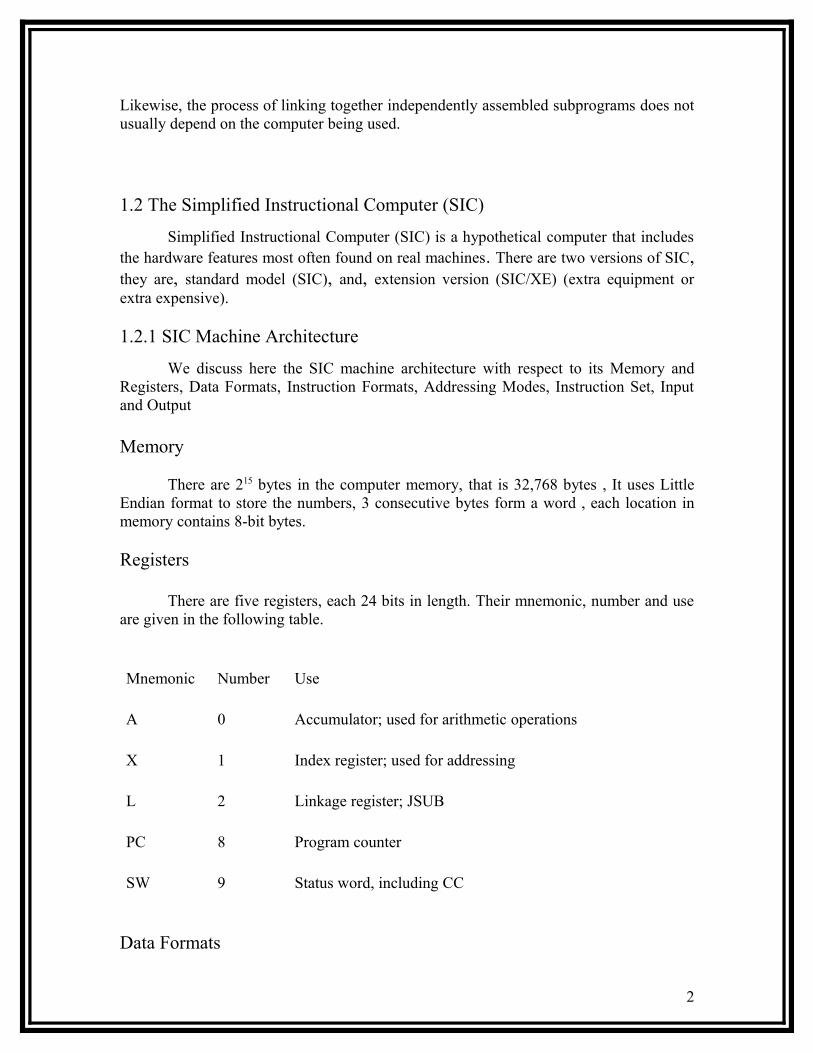
There are five registers, each 24 bits in length. Their mnemonic, number and use are given in the following table.
Mnemonic Number Use
A 0 Accumulator; used for arithmetic operations
X 1 Index register; used for addressing
L 2 Linkage register; JSUB
PC 8 Program counter
SW 9 Status word, including CC
Data Formats
2
Integers are stored as 24-bit binary numbers , 2’s complement representation is used for negative values, characters are stored using their 8-bit ASCII codes, No floating-point hardware on the standard version of SIC.Instruction Formats
Opcode(8) x Address (15)
All machine instructions on the standard version of SIC have the 24-bit format as shown above
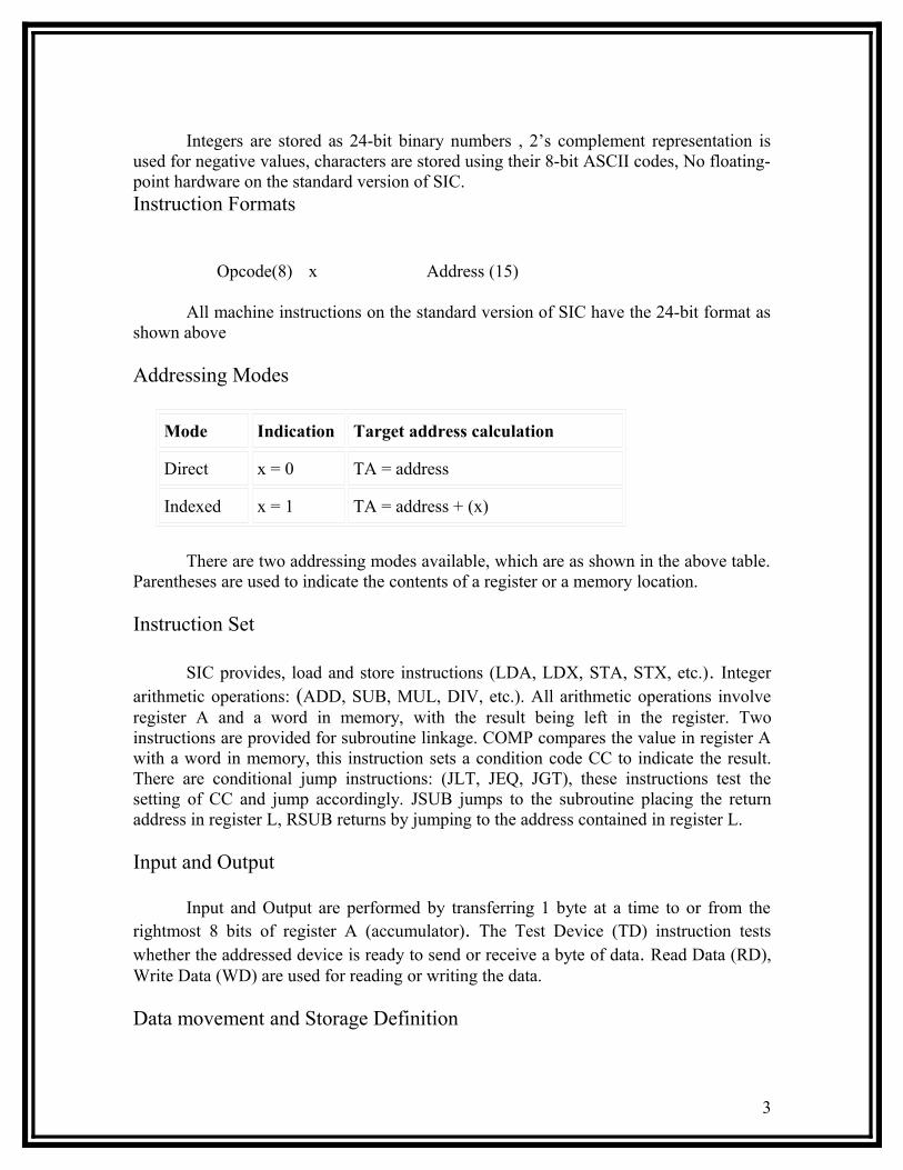
Addressing Modes
Mode Indication Target address calculation
Direct x = 0 TA = address
Indexed x = 1 TA = address + (x)
There are two addressing modes available, which are as shown in the above table. Parentheses are used to indicate the contents of a register or a memory location.
Instruction Set
SIC provides, load and store instructions (LDA, LDX, STA, STX, etc.). Integer arithmetic operations: (ADD, SUB, MUL, DIV, etc.). All arithmetic operations involve register A and a word in memory, with the result being left in the register. Two instructions are provided for subroutine linkage. COMP compares the value in register A with a word in memory, this instruction sets a condition code CC to indicate the result. There are conditional jump instructions: (JLT, JEQ, JGT), these instructions test the setting of CC and jump accordingly. JSUB jumps to the subroutine placing the return address in register L, RSUB returns by jumping to the address contained in register L.
Input and Output
Input and Output are performed by transferring 1 byte at a time to or from the rightmost 8 bits of register A (accumulator). The Test Device (TD) instruction tests whether the addressed device is ready to send or receive a byte of data. Read Data (RD), Write Data (WD) are used for reading or writing the data.
Data movement and Storage Definition
3

LDA, STA, LDL, STL, LDX, STX ( A- Accumulator, L – Linkage Register, X – Index Register), all uses 3-byte word. LDCH, STCH associated with characters uses 1-byte. There are no memory-memory move instructions.
Storage definitions are
• WORD - ONE-WORD CONSTANT• RESW - ONE-WORD VARIABLE• BYTE - ONE-BYTE CONSTANT• RESB - ONE-BYTE VARIABLE
Example Programs (SIC)
Example 1(Simple data and character movement operation)
LDA FIVE STA ALPHA LDCH CHARZ
STCH C1 .ALPHA RESW 1FIVE WORD 5CHARZ BYTE C’Z’C1 RESB 1
Example 2( Arithmetic operations)
LDA ALPHA ADD INCR SUB ONE STA BEETA …….. …….. …….. ……..ONE WORD 1ALPHA RESW 1BEETA RESW 1INCR RESW 1
Example 3(Looping and Indexing operation)
LDX ZERO : X = 0 MOVECH LDCH STR1, X : LOAD A FROM STR1
4

STCH STR2, X : STORE A TO STR2 TIX ELEVEN : ADD 1 TO X, TEST JLT MOVECH . . .STR1 BYTE C ‘HELLO WORLD’STR2 RESB 11ZERO WORD 0ELEVEN WORD 11
Example 4( Input and Output operation)
INLOOP TD INDEV : TEST INPUT DEVICE JEQ INLOOP : LOOP UNTIL DEVICE IS READY RD INDEV : READ ONE BYTE INTO A STCH DATA : STORE A TO DATA . .OUTLP TD OUTDEV : TEST OUTPUT DEVICE JEQ OUTLP : LOOP UNTIL DEVICE IS READY LDCH DATA : LOAD DATA INTO A WD OUTDEV : WRITE A TO OUTPUT DEVICE . .INDEV BYTE X ‘F5’ : INPUT DEVICE NUMBEROUTDEV BYTE X ‘08’ : OUTPUT DEVICE NUMBERDATA RESB 1 : ONE-BYTE VARIABLE
Example 5 (To transfer two hundred bytes of data from input device to memory)
LDX ZEROCLOOP TD INDEV JEQ CLOOP RD INDEV STCH RECORD, X TIX B200 JLT CLOOP . .INDEV BYTE X ‘F5’RECORD RESB 200ZERO WORD 0
5

B200 WORD 200
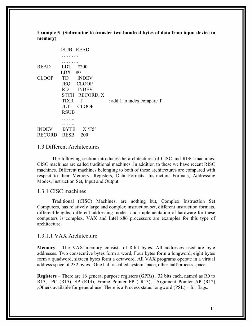
Example 6 (Subroutine to transfer two hundred bytes of data from input device to memory)
JSUB READ …………. ………….READ LDX ZEROCLOOP TD INDEV JEQ CLOOP RD INDEV STCH RECORD, X TIX B200 : add 1 to index compare 200 (B200) JLT CLOOP RSUB …….. ……..INDEV BYTE X ‘F5’RECORD RESB 200ZERO WORD 0B200 WORD 200
1.2.2 SIC/XE Machine Architecture
Memory
Maximum memory available on a SIC/XE system is 1 Megabyte (220 bytes)
Registers
Additional B, S, T, and F registers are provided by SIC/XE, in addition to the registers of SIC
Mnemonic Number Special use
B 3 Base registerS 4 General working registerT 5 General working registerF 6 Floating-point accumulator (48 bits)
Floating-point data type
6

There is a 48-bit floating-point data type, F*2(e-1024)
1 11 36
s exponent fraction
Instruction Formats
The new set of instruction formats for SIC/XE machine architecture are as follows. Format 1 (1 byte): contains only operation code (straight from table). Format 2 (2 bytes): first eight bits for operation code, next four for register 1 and following four for register 2. The numbers for the registers go according to the numbers indicated at the registers section (ie, register T is replaced by hex 5, F is replaced by hex 6). Format 3 (3 bytes): First 6 bits contain operation code, next 6 bits contain flags, last 12 bits contain displacement for the address of the operand. Operation code uses only 6 bits, thus the second hex digit will be affected by the values of the first two flags (n and i). The flags, in order, are: n, i, x, b, p, and e. Its functionality is explained in the next section. The last flag e indicates the instruction format (0 for 3 and 1 for 4). Format 4 (4 bytes): same as format 3 with an extra 2 hex digits (8 bits) for addresses that require more than 12 bits to be represented. Format 1 (1 byte)
8
op
Format 2 (2 bytes)
8 4 4
op r1 r2
Formats 1 and 2 are instructions do not reference memory at all
Format 3 (3 bytes)
6 1 1 1 1 1 1 12
op n i x b p e disp
7
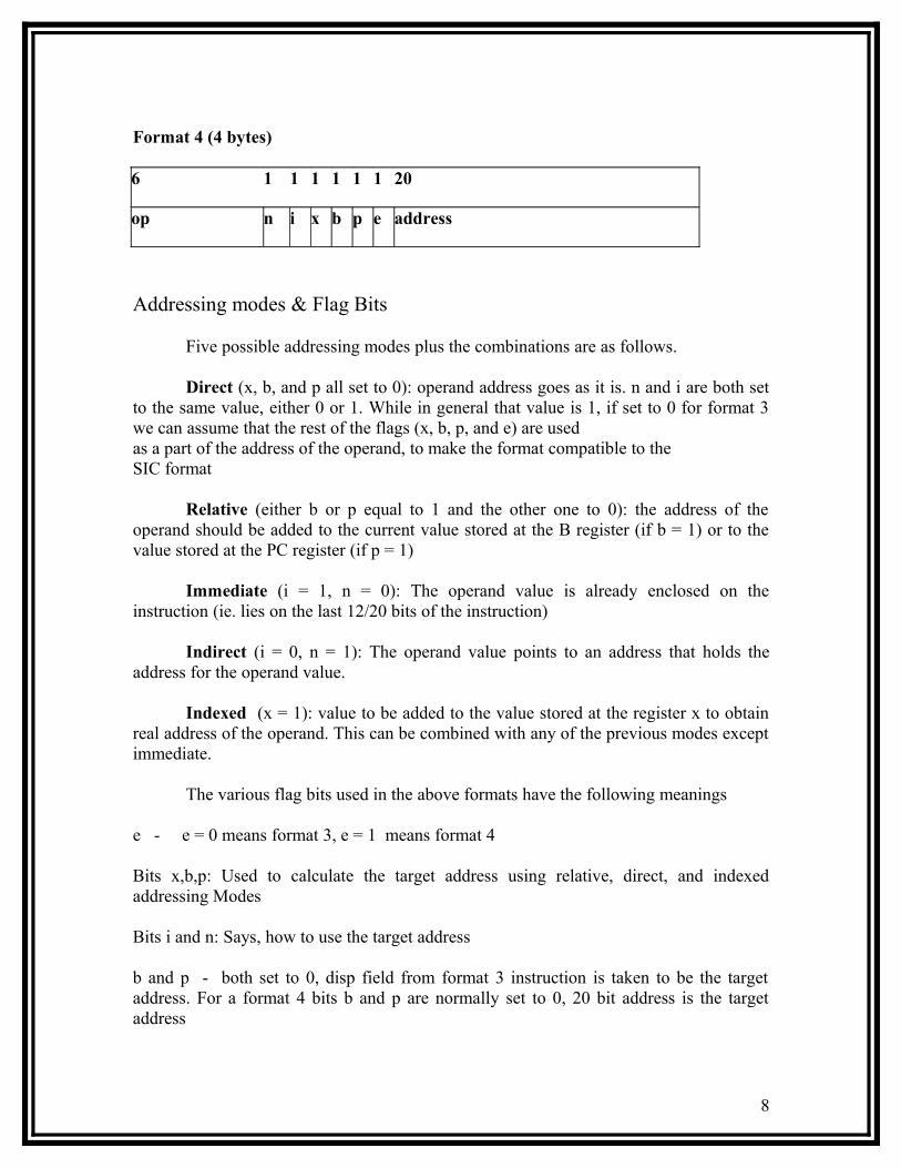
Format 4 (4 bytes)
6 1 1 1 1 1 1 20
op n i x b p e address
Addressing modes & Flag Bits
Five possible addressing modes plus the combinations are as follows.
Direct (x, b, and p all set to 0): operand address goes as it is. n and i are both set to the same value, either 0 or 1. While in general that value is 1, if set to 0 for format 3 we can assume that the rest of the flags (x, b, p, and e) are usedas a part of the address of the operand, to make the format compatible to theSIC format
Relative (either b or p equal to 1 and the other one to 0): the address of the operand should be added to the current value stored at the B register (if b = 1) or to the value stored at the PC register (if p = 1)
Immediate (i = 1, n = 0): The operand value is already enclosed on the instruction (ie. lies on the last 12/20 bits of the instruction)
Indirect (i = 0, n = 1): The operand value points to an address that holds the address for the operand value.
Indexed (x = 1): value to be added to the value stored at the register x to obtain real address of the operand. This can be combined with any of the previous modes except immediate.
The various flag bits used in the above formats have the following meanings
e - e = 0 means format 3, e = 1 means format 4
Bits x,b,p: Used to calculate the target address using relative, direct, and indexed addressing Modes
Bits i and n: Says, how to use the target address
b and p - both set to 0, disp field from format 3 instruction is taken to be the target address. For a format 4 bits b and p are normally set to 0, 20 bit address is the target address
8
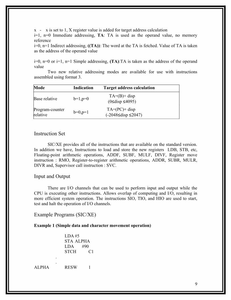
x - x is set to 1, X register value is added for target address calculationi=1, n=0 Immediate addressing, TA: TA is used as the operand value, no memory referencei=0, n=1 Indirect addressing, ((TA)): The word at the TA is fetched. Value of TA is taken as the address of the operand value
i=0, n=0 or i=1, n=1 Simple addressing, (TA):TA is taken as the address of the operand value
Two new relative addressing modes are available for use with instructions assembled using format 3.
Mode Indication Target address calculation
Base relative b=1,p=0 TA=(B)+ disp (0≤disp ≤4095)
Program-counter relative b=0,p=1 TA=(PC)+ disp
(-2048≤disp ≤2047)
Instruction Set
SIC/XE provides all of the instructions that are available on the standard version. In addition we have, Instructions to load and store the new registers LDB, STB, etc, Floating-point arithmetic operations, ADDF, SUBF, MULF, DIVF, Register move instruction : RMO, Register-to-register arithmetic operations, ADDR, SUBR, MULR, DIVR and, Supervisor call instruction : SVC.
Input and Output
There are I/O channels that can be used to perform input and output while the CPU is executing other instructions. Allows overlap of computing and I/O, resulting in more efficient system operation. The instructions SIO, TIO, and HIO are used to start, test and halt the operation of I/O channels.
Example Programs (SIC/XE)
Example 1 (Simple data and character movement operation)
LDA #5 STA ALPHA LDA #90
STCH C1 . .ALPHA RESW 1
9

C1 RESB 1Example 2(Arithmetic operations)
LDS INCR LDA ALPHA ADD S,A SUB #1 STA BEETA …………. …………..ALPHA RESW 1BEETA RESW 1INCR RESW 1
Example 3(Looping and Indexing operation)
LDT #11 LDX #0 : X = 0 MOVECH LDCH STR1, X : LOAD A FROM STR1 STCH STR2, X : STORE A TO STR2 TIXR T : ADD 1 TO X, TEST (T) JLT MOVECH ………. ………. ……… STR1 BYTE C ‘HELLO WORLD’ STR2 RESB 11
Example 4 (To transfer two hundred bytes of data from input device to memory)
LDT #200 LDX #0CLOOP TD INDEV JEQ CLOOP RD INDEV STCH RECORD, X TIXR T JLT CLOOP . .INDEV BYTE X ‘F5’RECORD RESB 200
10
Example 5 (Subroutine to transfer two hundred bytes of data from input device to memory)
JSUB READ ………. ……….READ LDT #200 LDX #0CLOOP TD INDEV JEQ CLOOP RD INDEV STCH RECORD, X TIXR T : add 1 to index compare T JLT CLOOP RSUB …….. ……..INDEV BYTE X ‘F5’RECORD RESB 200
1.3 Different Architectures
The following section introduces the architectures of CISC and RISC machines. CISC machines are called traditional machines. In addition to these we have recent RISC machines. Different machines belonging to both of these architectures are compared with respect to their Memory, Registers, Data Formats, Instruction Formats, Addressing Modes, Instruction Set, Input and Output
1.3.1 CISC machines
Traditional (CISC) Machines, are nothing but, Complex Instruction Set Computers, has relatively large and complex instruction set, different instruction formats, different lengths, different addressing modes, and implementation of hardware for these computers is complex. VAX and Intel x86 processors are examples for this type of architecture.
1.3.1.1 VAX Architecture
Memory - The VAX memory consists of 8-bit bytes. All addresses used are byte addresses. Two consecutive bytes form a word, Four bytes form a longword, eight bytes form a quadword, sixteen bytes form a octaword. All VAX programs operate in a virtual address space of 232 bytes , One half is called system space, other half process space.
Registers – There are 16 general purpose registers (GPRs) , 32 bits each, named as R0 to R15, PC (R15), SP (R14), Frame Pointer FP ( R13), Argument Pointer AP (R12) ,Others available for general use. There is a Process status longword (PSL) – for flags.
11
Data Formats - Integers are stored as binary numbers in byte, word, longword, quadword, octaword. 2’s complement notation is used for storing negative numbers. Characters are stored as 8-bit ASCII codes. Four different floating-point data formats are also available.
Instruction Formats - VAX architecture uses variable-length instruction formats – op code 1 or 2 bytes, maximum of 6 operand specifiers depending on type of instruction. Tabak – Advanced Microprocessors (2nd edition) McGraw-Hill, 1995, gives more information.
Addressing Modes - VAX provides a large number of addressing modes. They are Register mode, register deferred mode, autoincrement, autodecrement, base relative, program-counter relative, indexed, indirect, and immediate.
Instruction Set – Instructions are symmetric with respect to data type - Uses prefix – type of operation, suffix – type of operands, a modifier – number of operands. For example, ADDW2 - add, word length, 2 operands, MULL3 - multiply, longwords, 3 operands CVTCL - conversion from word to longword. VAX also provides instructions to load and store multiple registers.
Input and Output - Uses I/O device controllers. Device control registers are mapped to separate I/O space. Software routines and memory management routines are used for input/output operations.
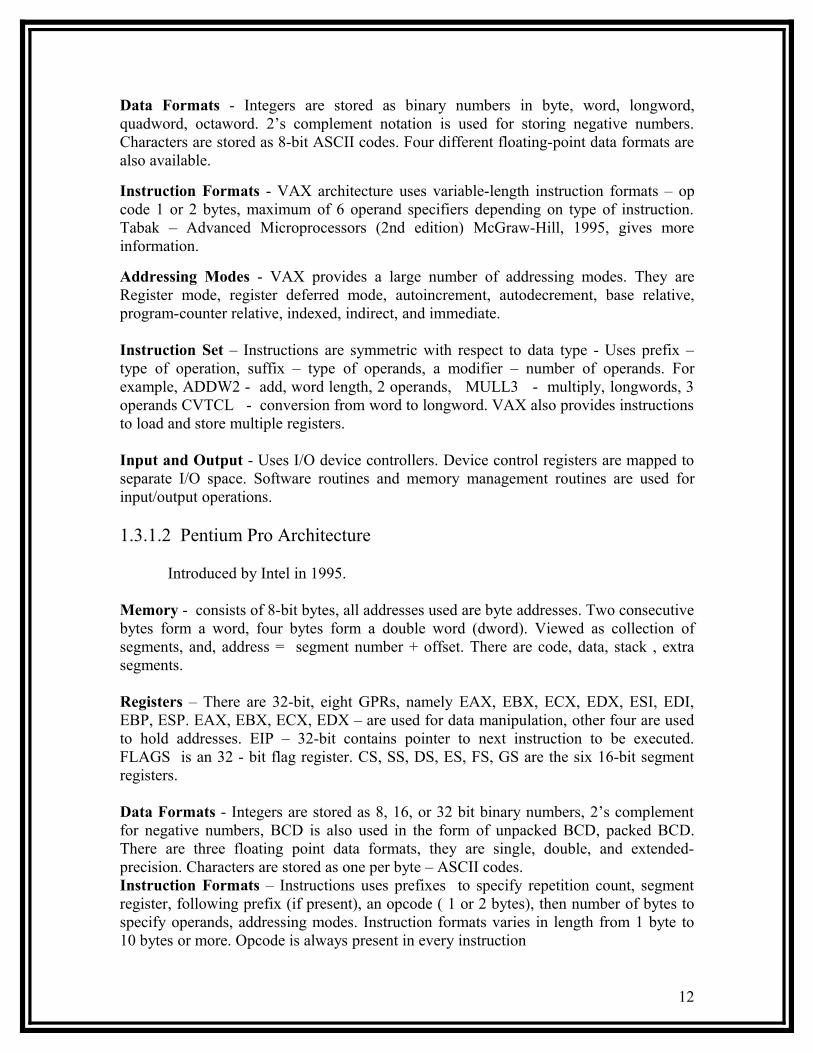
1.3.1.2 Pentium Pro Architecture
Introduced by Intel in 1995.
Memory - consists of 8-bit bytes, all addresses used are byte addresses. Two consecutive bytes form a word, four bytes form a double word (dword). Viewed as collection of segments, and, address = segment number + offset. There are code, data, stack , extra segments.
Registers – There are 32-bit, eight GPRs, namely EAX, EBX, ECX, EDX, ESI, EDI, EBP, ESP. EAX, EBX, ECX, EDX – are used for data manipulation, other four are used to hold addresses. EIP – 32-bit contains pointer to next instruction to be executed. FLAGS is an 32 - bit flag register. CS, SS, DS, ES, FS, GS are the six 16-bit segment registers.
Data Formats - Integers are stored as 8, 16, or 32 bit binary numbers, 2’s complement for negative numbers, BCD is also used in the form of unpacked BCD, packed BCD. There are three floating point data formats, they are single, double, and extended-precision. Characters are stored as one per byte – ASCII codes.Instruction Formats – Instructions uses prefixes to specify repetition count, segment register, following prefix (if present), an opcode ( 1 or 2 bytes), then number of bytes to specify operands, addressing modes. Instruction formats varies in length from 1 byte to 10 bytes or more. Opcode is always present in every instruction
12
Addressing Modes - A large number of addressing modes are available. They are immediate mode, register mode, direct mode, and relative mode. Use of base register, index register with displacement is also possible.
Instruction Set – This architecture has a large and complex instruction set, approximately 400 different machine instructions. Each instruction may have one, two or three operands. For example Register-to-register, register-to-memory, memory-to-memory, string manipulation, etc…are the some the instructions.
Input and Output - Input is from an I/O port into register EAX. Output is from EAX to an I/O port
1.3.2 RISC Machines
RISC means Reduced Instruction Set Computers. These machines are intended to simplify the design of processors. They have Greater reliability, faster execution and less expensive processors. And also they have standard and fixed instruction length. Number of machine instructions, instruction formats, and addressing modes relatively small. UltraSPARC Architecture and Cray T3E Architecture are examples of RISC machines.
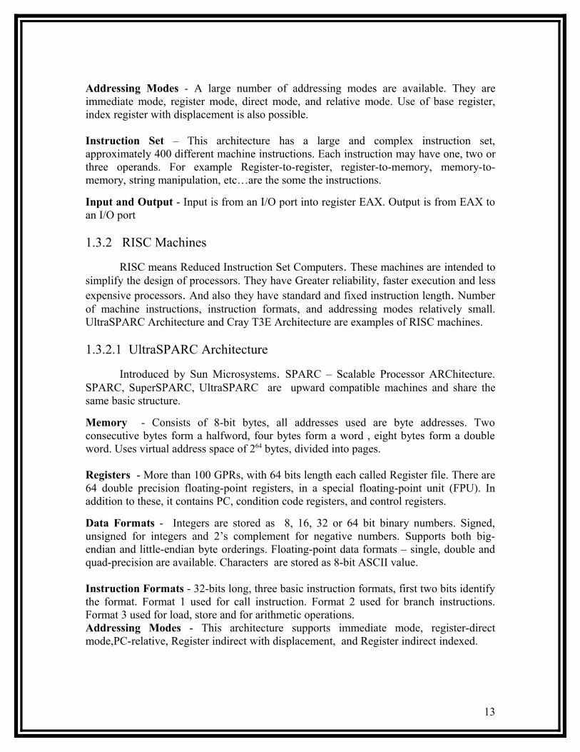
1.3.2.1 UltraSPARC Architecture
Introduced by Sun Microsystems. SPARC – Scalable Processor ARChitecture. SPARC, SuperSPARC, UltraSPARC are upward compatible machines and share the same basic structure.
Memory - Consists of 8-bit bytes, all addresses used are byte addresses. Two consecutive bytes form a halfword, four bytes form a word , eight bytes form a double word. Uses virtual address space of 264 bytes, divided into pages.
Registers - More than 100 GPRs, with 64 bits length each called Register file. There are 64 double precision floating-point registers, in a special floating-point unit (FPU). In addition to these, it contains PC, condition code registers, and control registers.
Data Formats - Integers are stored as 8, 16, 32 or 64 bit binary numbers. Signed, unsigned for integers and 2’s complement for negative numbers. Supports both big-endian and little-endian byte orderings. Floating-point data formats – single, double and quad-precision are available. Characters are stored as 8-bit ASCII value.
Instruction Formats - 32-bits long, three basic instruction formats, first two bits identify the format. Format 1 used for call instruction. Format 2 used for branch instructions. Format 3 used for load, store and for arithmetic operations.Addressing Modes - This architecture supports immediate mode, register-direct mode,PC-relative, Register indirect with displacement, and Register indirect indexed.
13

Instruction Set – It has fewer than 100 machine instructions. The only instructions that access memory are loads and stores. All other instructions are register-to-register operations. Instruction execution is pipelined – this results in faster execution, and hence speed increases.
Input and Output - Communication through I/O devices is accomplished through memory. A range of memory locations is logically replaced by device registers. When a load or store instruction refers to this device register area of memory, the corresponding device is activated. There are no special I/O instructions.
1.3.2.2 Cray T3E Architecture
Announced by Cray Research Inc., at the end of 1995 and is a massively parallel processing (MPP) system, contains a large number of processing elements (PEs), arranged in a three-dimensional network. Each PE consists of a DEC Alpha EV5 RISC processor, and local memory.
Memory - Each PE in T3E has its own local memory with a capacity of from 64 megabytes to 2 gigabytes, consists of 8-bit bytes, all addresses used are byte addresses. Two consecutive bytes form a word, four bytes form a longword, eight bytes form a quadword.
Registers – There are 32 general purpose registers(GPRs), with 64 bits length each called R0 through R31, contains value zero always. In addition to these, it has 32 floating-point registers, 64 bits long, and 64-bit PC, status , and control registers.
Data Formats - Integers are stored as long and quadword binary numbers. 2’s complement notation for negative numbers. Supports only little-endian byte orderings. Two different floating-point data formats – VAX and IEEE standard. Characters stored as 8-bit ASCII value.
Instruction Formats - 32-bits long, five basic instruction formats. First six bits always identify the opcode.
Addressing Modes - This architecture supports, immediate mode, register-direct mode, PC-relative, and Register indirect with displacement.
Instruction Set - Has approximately 130 machine instructions. There are no byte or word load and store instructions. Smith and Weiss – “PowerPC 601 and Alpha 21064: A Tale of TWO RISCs “ – Gives more information.
Input and Output - Communication through I/O devices is accomplished through multiple ports and I/O channels. Channels are integrated into the network that interconnects the processing elements. All channels are accessible and controllable from all PEs.
____________
14

Chapter 2Assembler Design
Assembler is system software which is used to convert an assembly language program to its equivalent object code. The input to the assembler is a source code written in assembly language (using mnemonics) and the output is the object code. The design of an assembler depends upon the machine architecture as the language used is mnemonic language.
1. Basic Assembler Functions:
The basic assembler functions are:• Translating mnemonic language code to its equivalent object code.• Assigning machine addresses to symbolic labels.
• The design of assembler can be to perform the following:– Scanning (tokenizing)– Parsing (validating the instructions)– Creating the symbol table – Resolving the forward references– Converting into the machine language
• The design of assembler in other words:– Convert mnemonic operation codes to their machine language equivalents– Convert symbolic operands to their equivalent machine addresses– Decide the proper instruction format Convert the data constants to internal machine representations– Write the object program and the assembly listing
So for the design of the assembler we need to concentrate on the machine architecture of the SIC/XE machine. We need to identify the algorithms and the various data structures to be used. According to the above required steps for assembling the assembler also has to handle assembler directives, these do not generate the object code but directs the assembler to perform certain operation. These directives are:
• SIC Assembler Directive:– START: Specify name & starting address.– END: End of the program, specify the first execution instruction.
15
– BYTE, WORD, RESB, RESW– End of record: a null char(00)End of file: a zero length record
The assembler design can be done:• Single pass assembler• Multi-pass assembler
Single-pass Assembler:
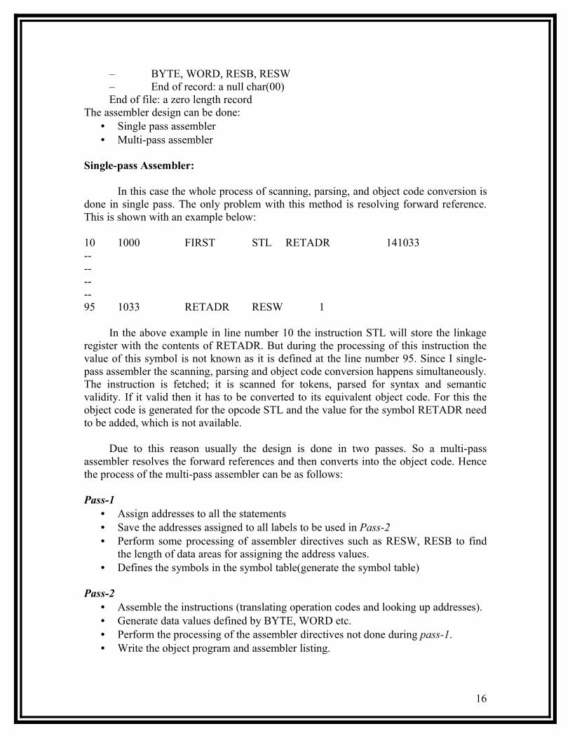
In this case the whole process of scanning, parsing, and object code conversion is done in single pass. The only problem with this method is resolving forward reference. This is shown with an example below:
10 1000 FIRST STL RETADR 141033--------95 1033 RETADR RESW 1
In the above example in line number 10 the instruction STL will store the linkage register with the contents of RETADR. But during the processing of this instruction the value of this symbol is not known as it is defined at the line number 95. Since I single-pass assembler the scanning, parsing and object code conversion happens simultaneously. The instruction is fetched; it is scanned for tokens, parsed for syntax and semantic validity. If it valid then it has to be converted to its equivalent object code. For this the object code is generated for the opcode STL and the value for the symbol RETADR need to be added, which is not available.
Due to this reason usually the design is done in two passes. So a multi-pass assembler resolves the forward references and then converts into the object code. Hence the process of the multi-pass assembler can be as follows:
Pass-1• Assign addresses to all the statements• Save the addresses assigned to all labels to be used in Pass-2• Perform some processing of assembler directives such as RESW, RESB to find
the length of data areas for assigning the address values.• Defines the symbols in the symbol table(generate the symbol table)
Pass-2• Assemble the instructions (translating operation codes and looking up addresses).• Generate data values defined by BYTE, WORD etc.• Perform the processing of the assembler directives not done during pass-1.• Write the object program and assembler listing.
16

Assembler Design:
The most important things which need to be concentrated is the generation of Symbol table and resolving forward references.
• Symbol Table:– This is created during pass 1– All the labels of the instructions are symbols– Table has entry for symbol name, address value.
• Forward reference:– Symbols that are defined in the later part of the program are called
forward referencing.– There will not be any address value for such symbols in the symbol table
in pass 1.
Example Program:
The example program considered here has a main module, two subroutines • Purpose of example program
- Reads records from input device (code F1) - Copies them to output device (code 05) - At the end of the file, writes EOF on the output device, then RSUB to the operating system
• Data transfer (RD, WD) -A buffer is used to store record -Buffering is necessary for different I/O rates -The end of each record is marked with a null character (00)16 -The end of the file is indicated by a zero-length record
• Subroutines (JSUB, RSUB) -RDREC, WRREC -Save link register first before nested jump
17

18

The first column shows the line number for that instruction, second column shows the addresses allocated to each instruction. The third column indicates the labels given to the statement, and is followed by the instruction consisting of opcode and operand. The last column gives the equivalent object code.
The object code later will be loaded into memory for execution. The simple object program we use contains three types of records:
• Header record- Col. 1 H- Col. 2~7 Program name- Col. 8~13 Starting address of object program (hex)- Col. 14~19 Length of object program in bytes (hex)
• Text record- Col. 1 T- Col. 2~7 Starting address for object code in this record (hex)- Col. 8~9 Length of object code in this record in bytes (hex)- Col. 10~69 Object code, represented in hex (2 col. per byte)
• End record- Col.1 E- Col.2~7 Address of first executable instruction in object program (hex)
“^” is only for separation only
Object code for the example program:
Session –II1. Simple SIC Assembler
19

The program below is shown with the object code generated. The column named LOC gives the machine addresses of each part of the assembled program (assuming the program is starting at location 1000). The translation of the source program to the object program requires us to accomplish the following functions:
1. Convert the mnemonic operation codes to their machine language equivalent.2. Convert symbolic operands to their equivalent machine addresses.3. Build the machine instructions in the proper format.4. Convert the data constants specified in the source program into their internal
machine representations in the proper format.5. Write the object program and assembly listing.
All these steps except the second can be performed by sequential processing of the source program, one line at a time. Consider the instruction 10 1000 LDA ALPHA 00-----
This instruction contains the forward reference, i.e. the symbol ALPHA is used is not yet defined. If the program is processed ( scanning and parsing and object code conversion) is done line-by-line, we will be unable to resolve the address of this symbol. Due to this problem most of the assemblers are designed to process the program in two passes.
In addition to the translation to object program, the assembler has to take care of handling assembler directive. These directives do not have object conversion but gives direction to the assembler to perform some function. Examples of directives are the statements like BYTE and WORD, which directs the assembler to reserve memory locations without generating data values. The other directives are START which indicates the beginning of the program and END indicating the end of the program.
The assembled program will be loaded into memory for execution. The simple object program contains three types of records: Header record, Text record and end record. The header record contains the starting address and length. Text record contains the translated instructions and data of the program, together with an indication of the addresses where these are to be loaded. The end record marks the end of the object program and specifies the address where the execution is to begin.
The format of each record is as given below.
Header record:Col 1 HCol. 2-7 Program nameCol 8-13 Starting address of object program (hexadecimal)Col 14-19 Length of object program in bytes (hexadecimal)
Text record:Col. 1 T
20

Col 2-7. Starting address for object code in this record (hexadecimal)Col 8-9 Length off object code in this record in bytes (hexadecimal)Col 10-69 Object code, represented in hexadecimal (2 columns per byte of object code)
End record:Col. 1 ECol 2-7 Address of first executable instruction in object program (hexadecimal)
The assembler can be designed either as a single pass assembler or as a two pass assembler. The general description of both passes is as given below:
• Pass 1 (define symbols)– Assign addresses to all statements in the program– Save the addresses assigned to all labels for use in Pass 2– Perform assembler directives, including those for address assignment,
such as BYTE and RESW• Pass 2 (assemble instructions and generate object program)
– Assemble instructions (generate opcode and look up addresses)– Generate data values defined by BYTE, WORD– Perform processing of assembler directives not done during Pass 1– Write the object program and the assembly listing
2. Algorithms and Data structure
The simple assembler uses two major internal data structures: the operation Code Table (OPTAB) and the Symbol Table (SYMTAB).
OPTAB: It is used to lookup mnemonic operation codes and translates them to their machine language equivalents. In more complex assemblers the table also contains information about instruction format and length. In pass 1 the OPTAB is used to look up and validate the operation code in the source program. In pass 2, it is used to translate the operation codes to machine language. In simple SIC machine this process can be performed in either in pass 1 or in pass 2. But for machine like SIC/XE that has instructions of different lengths, we must search OPTAB in the first pass to find the instruction length for incrementing LOCCTR. In pass 2 we take the information from OPTAB to tell us which instruction format to use in assembling the instruction, and any peculiarities of the object code instruction.
OPTAB is usually organized as a hash table, with mnemonic operation code as the key. The hash table organization is particularly appropriate, since it provides fast retrieval with a minimum of searching. Most of the cases the OPTAB is a static table- that is, entries are not normally added to or deleted from it. In such cases it is possible to
21

design a special hashing function or other data structure to give optimum performance for the particular set of keys being stored.
SYMTAB: This table includes the name and value for each label in the source program, together with flags to indicate the error conditions (e.g., if a symbol is defined in two different places).
During Pass 1: labels are entered into the symbol table along with their assigned address value as they are encountered. All the symbols address value should get resolved at the pass 1.
During Pass 2: Symbols used as operands are looked up the symbol table to obtain the address value to be inserted in the assembled instructions.
SYMTAB is usually organized as a hash table for efficiency of insertion and retrieval. Since entries are rarely deleted, efficiency of deletion is the important criteria for optimization.
Both pass 1 and pass 2 require reading the source program. Apart from this an intermediate file is created by pass 1 that contains each source statement together with its assigned address, error indicators, etc. This file is one of the inputs to the pass 2. A copy of the source program is also an input to the pass 2, which is used to retain the operations that may be performed during pass 1 (such as scanning the operation field for symbols and addressing flags), so that these need not be performed during pass 2. Similarly, pointers into OPTAB and SYMTAB is retained for each operation code and symbol used. This avoids need to repeat many of the table-searching operations.
LOCCTR: Apart from the SYMTAB and OPTAB, this is another important variable which helps in the assignment of the addresses. LOCCTR is initialized to the beginning address mentioned in the START statement of the program. After each statement is processed, the length of the assembled instruction is added to the LOCCTR to make it point to the next instruction. Whenever a label is encountered in an instruction the LOCCTR value gives the address to be associated with that label.
The Algorithm for Pass 1:
Begin read first input line if OPCODE = ‘START’ then begin save #[Operand] as starting addr initialize LOCCTR to starting address write line to intermediate file read next line end( if START) else initialize LOCCTR to 0
22
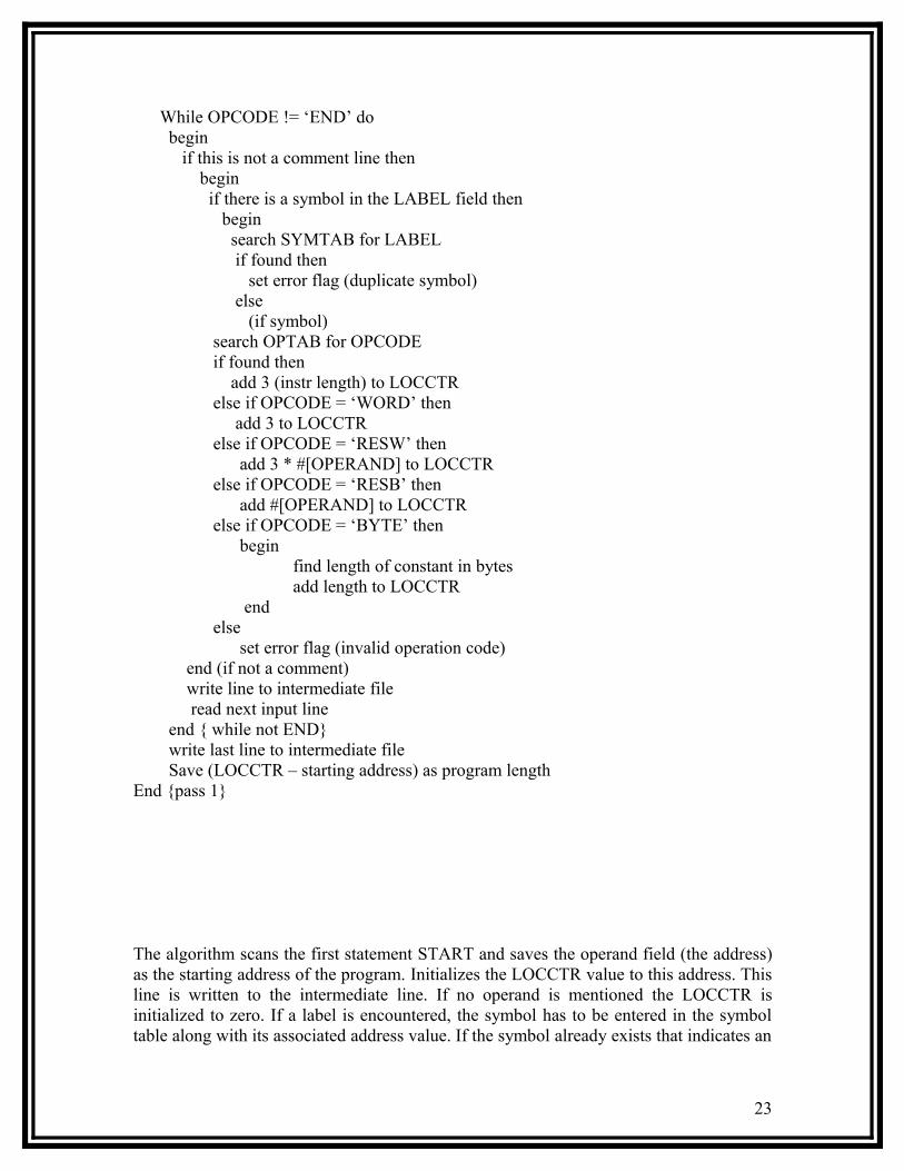
While OPCODE != ‘END’ do begin if this is not a comment line then begin if there is a symbol in the LABEL field then begin search SYMTAB for LABEL if found then set error flag (duplicate symbol) else (if symbol) search OPTAB for OPCODE if found then add 3 (instr length) to LOCCTR else if OPCODE = ‘WORD’ then add 3 to LOCCTR
else if OPCODE = ‘RESW’ then add 3 * #[OPERAND] to LOCCTR else if OPCODE = ‘RESB’ then add #[OPERAND] to LOCCTR else if OPCODE = ‘BYTE’ then begin find length of constant in bytes add length to LOCCTR end else set error flag (invalid operation code) end (if not a comment) write line to intermediate file read next input line end { while not END} write last line to intermediate file Save (LOCCTR – starting address) as program length
End {pass 1}
The algorithm scans the first statement START and saves the operand field (the address) as the starting address of the program. Initializes the LOCCTR value to this address. This line is written to the intermediate line. If no operand is mentioned the LOCCTR is initialized to zero. If a label is encountered, the symbol has to be entered in the symbol table along with its associated address value. If the symbol already exists that indicates an
23

entry of the same symbol already exists. So an error flag is set indicating a duplication of the symbol. It next checks for the mnemonic code, it searches for this code in the OPTAB. If found then the length of the instruction is added to the LOCCTR to make it point to the next instruction. If the opcode is the directive WORD it adds a value 3 to the LOCCTR. If it is RESW, it needs to add the number of data word to the LOCCTR. If it is BYTE it adds a value one to the LOCCTR, if RESB it adds number of bytes. If it is END directive then it is the end of the program it finds the length of the program by evaluating current LOCCTR – the starting address mentioned in the operand field of the END directive. Each processed line is written to the intermediate file.
The Algorithm for Pass 2:
Begin read 1st input line if OPCODE = ‘START’ then begin write listing line read next input line end write Header record to object program initialize 1st Text recordwhile OPCODE != ‘END’ do begin if this is not comment line then begin search OPTAB for OPCODE if found then begin if there is a symbol in OPERAND field then begin search SYMTAB for OPERAND field then if found then
begin store symbol value as operand address else begin store 0 as operand address set error flag (undefined symbol) end end (if symbol) else store 0 as operand address assemble the object code instruction else if OPCODE = ‘BYTE’ or ‘WORD” then convert constant to object code if object code doesn’t fit into current Text record then begin
24
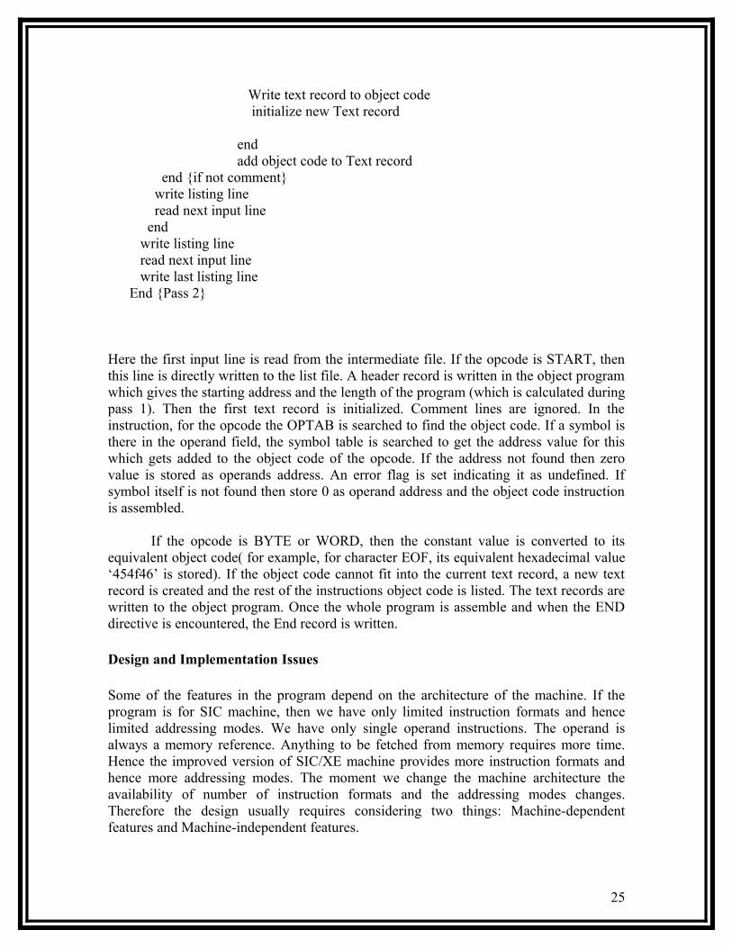
Write text record to object code initialize new Text record end add object code to Text record end {if not comment} write listing line read next input line end write listing line read next input line write last listing lineEnd {Pass 2}
Here the first input line is read from the intermediate file. If the opcode is START, then this line is directly written to the list file. A header record is written in the object program which gives the starting address and the length of the program (which is calculated during pass 1). Then the first text record is initialized. Comment lines are ignored. In the instruction, for the opcode the OPTAB is searched to find the object code. If a symbol is there in the operand field, the symbol table is searched to get the address value for this which gets added to the object code of the opcode. If the address not found then zero value is stored as operands address. An error flag is set indicating it as undefined. If symbol itself is not found then store 0 as operand address and the object code instruction is assembled.
If the opcode is BYTE or WORD, then the constant value is converted to its equivalent object code( for example, for character EOF, its equivalent hexadecimal value ‘454f46’ is stored). If the object code cannot fit into the current text record, a new text record is created and the rest of the instructions object code is listed. The text records are written to the object program. Once the whole program is assemble and when the END directive is encountered, the End record is written.
Design and Implementation Issues
Some of the features in the program depend on the architecture of the machine. If the program is for SIC machine, then we have only limited instruction formats and hence limited addressing modes. We have only single operand instructions. The operand is always a memory reference. Anything to be fetched from memory requires more time. Hence the improved version of SIC/XE machine provides more instruction formats and hence more addressing modes. The moment we change the machine architecture the availability of number of instruction formats and the addressing modes changes. Therefore the design usually requires considering two things: Machine-dependent features and Machine-independent features.
25

3. Machine-Dependent Features:
• Instruction formats and addressing modes• Program relocation
3.1 Instruction formats and Addressing Modes
The instruction formats depend on the memory organization and the size of the memory. In SIC machine the memory is byte addressable. Word size is 3 bytes. So the size of the memory is 212 bytes. Accordingly it supports only one instruction format. It has only two registers: register A and Index register. Therefore the addressing modes supported by this architecture are direct, indirect, and indexed. Whereas the memory of a SIC/XE machine is 220 bytes (1 MB). This supports four different types of instruction types, they are:
1 byte instruction 2 byte instruction 3 byte instruction 4 byte instruction
• Instructions can be:– Instructions involving register to register– Instructions with one operand in memory, the other in Accumulator
(Single operand instruction)– Extended instruction format
• Addressing Modes are:– Index Addressing(SIC): Opcode m, x– Indirect Addressing: Opcode @m– PC-relative: Opcode m– Base relative: Opcode m– Immediate addressing: Opcode #c
Translations for the Instruction involving Register-Register addressing mode:
During pass 1 the registers can be entered as part of the symbol table itself. The value for these registers is their equivalent numeric codes. During pass 2, these values are assembled along with the mnemonics object code. If required a separate table can be created with the register names and their equivalent numeric values.
Translation involving Register-Memory instructions:
In SIC/XE machine there are four instruction formats and five addressing modes. For formats and addressing modes refer chapter 1.
Among the instruction formats, format -3 and format-4 instructions are Register-Memory type of instruction. One of the operand is always in a register and the other
26

operand is in the memory. The addressing mode tells us the way in which the operand from the memory is to be fetched.
There are two ways: Program-counter relative and Base-relative. This addressing mode can be represented by either using format-3 type or format-4 type of instruction format. In format-3, the instruction has the opcode followed by a 12-bit displacement value in the address field. Where as in format-4 the instruction contains the mnemonic code followed by a 20-bit displacement value in the address field.
2. Program-Counter Relative: In this usually format-3 instruction format is used. The instruction contains the opcode followed by a 12-bit displacement value. The range of displacement values are from 0 -2048. This displacement (should be small enough to fit in a 12-bit field) value is added to the current contents of the program counter to get the target address of the operand required by the instruction. This is relative way of calculating the address of the operand relative to the program counter. Hence the displacement of the operand is relative to the current program counter value. The following example shows how the address is calculated:
3. Base-Relative Addressing Mode: in this mode the base register is used to mention the displacement value. Therefore the target address is
TA = (base) + displacement value
This addressing mode is used when the range of displacement value is not sufficient. Hence the operand is not relative to the instruction as in PC-relative addressing mode. Whenever this mode is used it is indicated by using a directive BASE. The moment the assembler encounters this directive the next instruction uses base-relative addressing mode to calculate the target address of the operand.
27
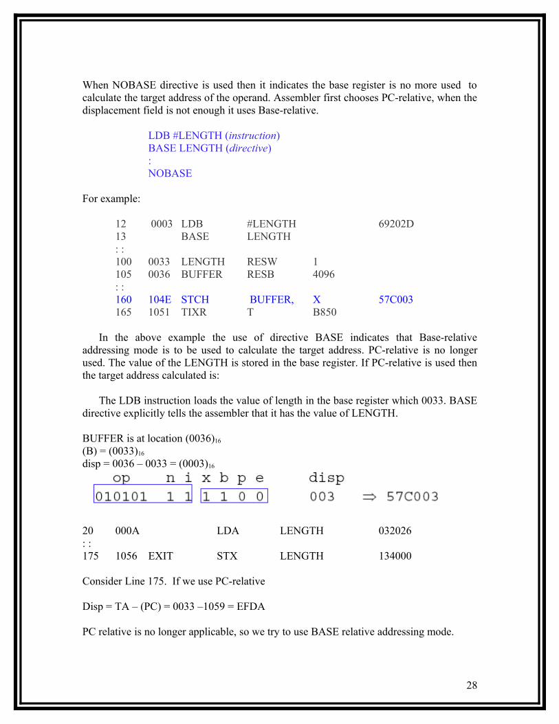
When NOBASE directive is used then it indicates the base register is no more used to calculate the target address of the operand. Assembler first chooses PC-relative, when the displacement field is not enough it uses Base-relative.
LDB #LENGTH (instruction)BASE LENGTH (directive):NOBASE
For example:
12 0003 LDB #LENGTH 69202D13 BASE LENGTH: :100 0033 LENGTH RESW 1105 0036 BUFFER RESB 4096: :160 104E STCH BUFFER, X 57C003165 1051 TIXR T B850
In the above example the use of directive BASE indicates that Base-relative addressing mode is to be used to calculate the target address. PC-relative is no longer used. The value of the LENGTH is stored in the base register. If PC-relative is used then the target address calculated is:
The LDB instruction loads the value of length in the base register which 0033. BASE directive explicitly tells the assembler that it has the value of LENGTH.
BUFFER is at location (0036)16
(B) = (0033)16
disp = 0036 – 0033 = (0003)16
20 000A LDA LENGTH 032026: :175 1056 EXIT STX LENGTH 134000
Consider Line 175. If we use PC-relative
Disp = TA – (PC) = 0033 –1059 = EFDA
PC relative is no longer applicable, so we try to use BASE relative addressing mode.
28

4. Immediate Addressing Mode
In this mode no memory reference is involved. If immediate mode is used the target address is the operand itself.
If the symbol is referred in the instruction as the immediate operand then it is immediate with PC-relative mode as shown in the example below:
5. Indirect and PC-relative mode:
In this type of instruction the symbol used in the instruction is the address of the location which contains the address of the operand. The address of this is found using PC-relative addressing mode. For example:
29

The instruction jumps the control to the address location RETADR which in turn has the address of the operand. If address of RETADR is 0030, the target address is then 0003 as calculated above.
3.2 Program Relocation
Sometimes it is required to load and run several programs at the same time. The system must be able to load these programs wherever there is place in the memory. Therefore the exact starting is not known until the load time.
Absolute Program
In this the address is mentioned during assembling itself. This is called Absolute Assembly. Consider the instruction:
55 101B LDA THREE 00102D
This statement says that the register A is loaded with the value stored at location 102D. Suppose it is decided to load and execute the program at location 2000 instead of location 1000. Then at address 102D the required value which needs to be loaded in the register A is no more available. The address also gets changed relative to the displacement of the program. Hence we need to make some changes in the address portion of the instruction so that we can load and execute the program at location 2000. Apart from the instruction which will undergo a change in their operand address value as the program load address changes. There exist some parts in the program which will remain same regardless of where the program is being loaded.
Since assembler will not know actual location where the program will get loaded, it cannot make the necessary changes in the addresses used in the program. However, the assembler identifies for the loader those parts of the program which need modification. An object program that has the information necessary to perform this kind of modification is called the relocatable program.
30

The above diagram shows the concept of relocation. Initially the program is loaded at location 0000. The instruction JSUB is loaded at location 0006. The address field of this instruction contains 01036, which is the address of the instruction labeled RDREC. The second figure shows that if the program is to be loaded at new location 5000. The address of the instruction JSUB gets modified to new location 6036. Likewise the third figure shows that if the program is relocated at location 7420, the JSUB instruction would need to be changed to 4B108456 that correspond to the new address of RDREC.
The only part of the program that require modification at load time are those that specify direct addresses. The rest of the instructions need not be modified. The instructions which doesn’t require modification are the ones that is not a memory address (immediate addressing) and PC-relative, Base-relative instructions. From the object program, it is not possible to distinguish the address and constant The assembler must keep some information to tell the loader. The object program that contains the modification record is called a relocatable program.
For an address label, its address is assigned relative to the start of the program (START 0). The assembler produces a Modification record to store the starting location and the length of the address field to be modified. The command for the loader must also be a part of the object program. The Modification has the following format:
Modification recordCol. 1 MCol. 2-7 Starting location of the address field to be modified, relative to the beginning of the program (Hex)Col. 8-9 Length of the address field to be modified, in half-bytes (Hex)
One modification record is created for each address to be modified The length is stored in half-bytes (4 bits) The starting location is the location of the byte containing the
31

leftmost bits of the address field to be modified. If the field contains an odd number of half-bytes, the starting location begins in the middle of the first byte.
In the above object code the red boxes indicate the addresses that need modifications. The object code lines at the end are the descriptions of the modification records for those instructions which need change if relocation occurs. M00000705 is the modification suggested for the statement at location 0007 and requires modification 5-half bytes. Similarly the remaining instructions indicate.
Assembler Design Session 4 & 5
3.2 Machine-Independent features:These are the features which do not depend on the architecture of the machine. These
are: Literals Expressions Program blocks Control sections
3.2.1 Literals:A literal is defined with a prefix = followed by a specification of the literal value.
Example:
45 001A ENDFIL LDA =C’EOF’ 032010--93 LTORG
002D * =C’EOF’ 454F46
The example above shows a 3-byte operand whose value is a character string EOF. The object code for the instruction is also mentioned. It shows the relative
32

displacement value of the location where this value is stored. In the example the value is at location (002D) and hence the displacement value is (010). As another example the given statement below shows a 1-byte literal with the hexadecimal value ‘05’.
215 1062 WLOOP TD =X’05’ E32011
It is important to understand the difference between a constant defined as a literal and a constant defined as an immediate operand. In case of literals the assembler generates the specified value as a constant at some other memory location In immediate mode the operand value is assembled as part of the instruction itself. Example
55 0020 LDA #03 010003
All the literal operands used in a program are gathered together into one or more literal pools. This is usually placed at the end of the program. The assembly listing of a program containing literals usually includes a listing of this literal pool, which shows the assigned addresses and the generated data values. In some cases it is placed at some other location in the object program. An assembler directive LTORG is used. Whenever the LTORG is encountered, it creates a literal pool that contains all the literal operands used since the beginning of the program. The literal pool definition is done after LTORG is encountered. It is better to place the literals close to the instructions.
A literal table is created for the literals which are used in the program. The literal table contains the literal name, operand value and length. The literal table is usually created as a hash table on the literal name.
Implementation of Literals:
During Pass-1:The literal encountered is searched in the literal table. If the literal already exists,
no action is taken; if it is not present, the literal is added to the LITTAB and for the address value it waits till it encounters LTORG for literal definition. When Pass 1 encounters a LTORG statement or the end of the program, the assembler makes a scan of the literal table. At this time each literal currently in the table is assigned an address. As addresses are assigned, the location counter is updated to reflect the number of bytes occupied by each literal.
During Pass-2:
The assembler searches the LITTAB for each literal encountered in the instruction and replaces it with its equivalent value as if these values are generated by BYTE or WORD. If a literal represents an address in the program, the assembler must generate a modification relocation for, if it all it gets affected due to relocation. The following figure shows the difference between the SYMTAB and LITTAB
33

3.2.2 Symbol-Defining Statements:
EQU Statement:Most assemblers provide an assembler directive that allows the programmer to
define symbols and specify their values. The directive used for this EQU (Equate). The general form of the statement is
Symbol EQU value
This statement defines the given symbol (i.e., entering in the SYMTAB) and assigning to it the value specified. The value can be a constant or an expression involving constants and any other symbol which is already defined. One common usage is to define symbolic names that can be used to improve readability in place of numeric values. For example
+LDT #4096
This loads the register T with immediate value 4096, this does not clearly what exactly this value indicates. If a statement is included as:
MAXLEN EQU 4096 and then+LDT #MAXLEN
Then it clearly indicates that the value of MAXLEN is some maximum length value. When the assembler encounters EQU statement, it enters the symbol MAXLEN along with its value in the symbol table. During LDT the assembler searches the SYMTAB for its entry and its equivalent value as the operand in the instruction. The object code generated is the same for both the options discussed, but is easier to understand. If the maximum length is changed from 4096 to 1024, it is difficult to change if it is mentioned as an immediate value wherever required in the instructions. We have to scan the whole program and make changes wherever 4096 is used. If we mention this value in the instruction through the symbol defined by EQU, we may not have to search the whole program but change only the value of MAXLENGTH in the EQU statement (only once).
34

Another common usage of EQU statement is for defining values for the general-purpose registers. The assembler can use the mnemonics for register usage like a-register A , X – index register and so on. But there are some instructions which requires numbers in place of names in the instructions. For example in the instruction RMO 0,1 instead of RMO A,X. The programmer can assign the numerical values to these registers using EQU directive.
A EQU 0X EQU 1 and so on
These statements will cause the symbols A, X, L… to be entered into the symbol table with their respective values. An instruction RMO A, X would then be allowed. As another usage if in a machine that has many general purpose registers named as R1, R2,…, some may be used as base register, some may be used as accumulator. Their usage may change from one program to another. In this case we can define these requirement using EQU statements.
BASE EQU R1INDEX EQU R2COUNT EQU R3
One restriction with the usage of EQU is whatever symbol occurs in the right hand side of the EQU should be predefined. For example, the following statement is not valid:
BETA EQU ALPHAALPHA RESW 1
As the symbol ALPHA is assigned to BETA before it is defined. The value of ALPHA is not known.
ORG Statement:
This directive can be used to indirectly assign values to the symbols. The directive is usually called ORG (for origin). Its general format is:
ORG valueWhere value is a constant or an expression involving constants and previously defined symbols. When this statement is encountered during assembly of a program, the assembler resets its location counter (LOCCTR) to the specified value. Since the values of symbols used as labels are taken from LOCCTR, the ORG statement will affect the values of all labels defined until the next ORG is encountered. ORG is used to control assignment storage in the object program. Sometimes altering the values may result in incorrect assembly.
ORG can be useful in label definition. Suppose we need to define a symbol table with the following structure:SYMBOL 6 BytesVALUE 3 Bytes
35

FLAG 2 Bytes
The table looks like the one given below.
The symbol field contains a 6-byte user-defined symbol; VALUE is a one-word representation of the value assigned to the symbol; FLAG is a 2-byte field specifies symbol type and other information. The space for the ttable can be reserved by the statement:
STAB RESB 1100
If we want to refer to the entries of the table using indexed addressing, place the offset value of the desired entry from the beginning of the table in the index register. To refer to the fields SYMBOL, VALUE, and FLAGS individually, we need to assign the values first as shown below:
SYMBOL EQU STABVALUE EQU STAB+6FLAGS EQU STAB+9
To retrieve the VALUE field from the table indicated by register X, we can write a statement:
LDA VALUE, X
The same thing can also be done using ORG statement in the following way:
STAB RESB 1100ORG STAB
SYMBOL RESB 6VALUE RESW 1FLAG RESB 2
ORG STAB+1100
36

The first statement allocates 1100 bytes of memory assigned to label STAB. In the second statement the ORG statement initializes the location counter to the value of STAB. Now the LOCCTR points to STAB. The next three lines assign appropriate memory storage to each of SYMBOL, VALUE and FLAG symbols. The last ORG statement reinitializes the LOCCTR to a new value after skipping the required number of memory for the table STAB (i.e., STAB+1100).
While using ORG, the symbol occurring in the statement should be predefined as is required in EQU statement. For example for the sequence of statements below:
ORG ALPHABYTE1 RESB 1BYTE2 RESB 1BYTE3 RESB 1
ORGALPHA RESB 1
The sequence could not be processed as the symbol used to assign the new location counter value is not defined. In first pass, as the assembler would not know what value to assign to ALPHA, the other symbol in the next lines also could not be defined in the symbol table. This is a kind of problem of the forward reference.
3.2.3 Expressions:
Assemblers also allow use of expressions in place of operands in the instruction. Each such expression must be evaluated to generate a single operand value or address. Assemblers generally arithmetic expressions formed according to the normal rules using arithmetic operators +, - *, /. Division is usually defined to produce an integer result. Individual terms may be constants, user-defined symbols, or special terms. The only special term used is * ( the current value of location counter) which indicates the value of the next unassigned memory location. Thus the statement
BUFFEND EQU *
Assigns a value to BUFFEND, which is the address of the next byte following the buffer area. Some values in the object program are relative to the beginning of the program and some are absolute (independent of the program location, like constants). Hence, expressions are classified as either absolute expression or relative expressions depending on the type of value they produce.
Absolute Expressions: The expression that uses only absolute terms is absolute expression. Absolute expression may contain relative term provided the relative terms occur in pairs with opposite signs for each pair. Example:
MAXLEN EQU BUFEND-BUFFER
37

In the above instruction the difference in the expression gives a value that does not depend on the location of the program and hence gives an absolute immaterial o the relocation of the program. The expression can have only absolute terms. Example:
MAXLEN EQU 1000
Relative Expressions: All the relative terms except one can be paired as described in “absolute”. The remaining unpaired relative term must have a positive sign. Example:
STAB EQU OPTAB + (BUFEND – BUFFER)
Handling the type of expressions: to find the type of expression, we must keep track the type of symbols used. This can be achieved by defining the type in the symbol table against each of the symbol as shown in the table below:
3.2.4 Program Blocks:
Program blocks allow the generated machine instructions and data to appear in the object program in a different order by Separating blocks for storing code, data, stack, and larger data block.Assembler Directive USE:
USE [blockname]At the beginning, statements are assumed to be part of the unnamed (default) block. If no USE statements are included, the entire program belongs to this single block. Each program block may actually contain several separate segments of the source program. Assemblers rearrange these segments to gather together the pieces of each block and assign address. Separate the program into blocks in a particular order. Large buffer area is moved to the end of the object program. Program readability is better if data areas are placed in the source program close to the statements that reference them.
In the example below three blocks are used :Default: executable instructions CDATA: all data areas that are less in lengthCBLKS: all data areas that consists of larger blocks of memory
38

Example Code
39
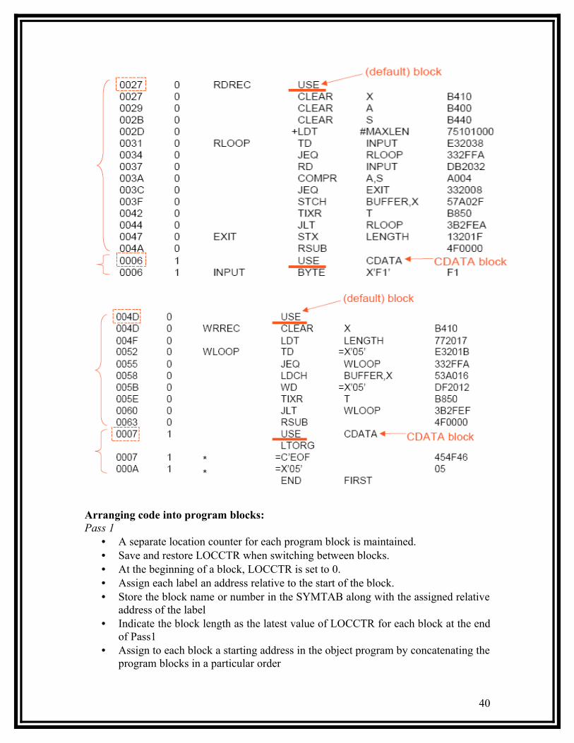
Arranging code into program blocks: Pass 1
• A separate location counter for each program block is maintained. • Save and restore LOCCTR when switching between blocks. • At the beginning of a block, LOCCTR is set to 0.• Assign each label an address relative to the start of the block.• Store the block name or number in the SYMTAB along with the assigned relative
address of the label• Indicate the block length as the latest value of LOCCTR for each block at the end
of Pass1• Assign to each block a starting address in the object program by concatenating the
program blocks in a particular order
40

Pass 2• Calculate the address for each symbol relative to the start of the object program
by adding The location of the symbol relative to the start of its block The starting address of this block
3.2.5 Control Sections:
A control section is a part of the program that maintains its identity after assembly; each control section can be loaded and relocated independently of the others. Different control sections are most often used for subroutines or other logical subdivisions. The programmer can assemble, load, and manipulate each of these control sections separately.
Because of this, there should be some means for linking control sections together. For example, instructions in one control section may refer to the data or instructions of other control sections. Since control sections are independently loaded and relocated, the assembler is unable to process these references in the usual way. Such references between different control sections are called external references.
The assembler generates the information about each of the external references that will allow the loader to perform the required linking. When a program is written using multiple control sections, the beginning of each of the control section is indicated by an assembler directive
– assembler directive: CSECTThe syntax
secname CSECT– separate location counter for each control section
Control sections differ from program blocks in that they are handled separately by the assembler. Symbols that are defined in one control section may not be used directly another control section; they must be identified as external reference for the loader to handle. The external references are indicated by two assembler directives:
EXTDEF (external Definition): It is the statement in a control section, names symbols that are defined in this
section but may be used by other control sections. Control section names do not need to be named in the EXTREF as they are automatically considered as external symbols.
EXTREF (external Reference):It names symbols that are used in this section but are defined in some other
control section.
41
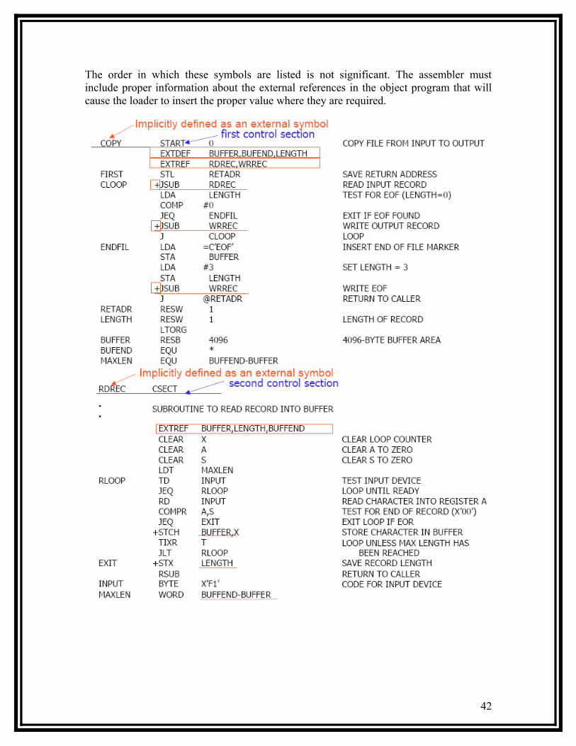
The order in which these symbols are listed is not significant. The assembler must include proper information about the external references in the object program that will cause the loader to insert the proper value where they are required.
42
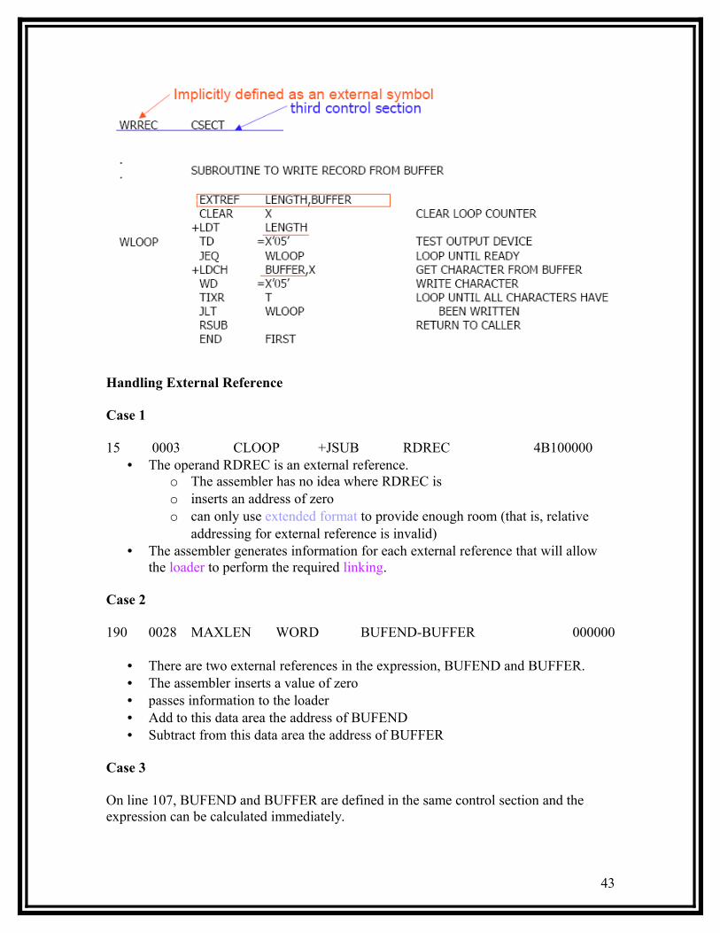
Handling External Reference
Case 1
15 0003 CLOOP +JSUB RDREC 4B100000• The operand RDREC is an external reference.
o The assembler has no idea where RDREC iso inserts an address of zeroo can only use extended format to provide enough room (that is, relative
addressing for external reference is invalid)• The assembler generates information for each external reference that will allow
the loader to perform the required linking.
Case 2
190 0028 MAXLEN WORD BUFEND-BUFFER 000000
• There are two external references in the expression, BUFEND and BUFFER.• The assembler inserts a value of zero• passes information to the loader• Add to this data area the address of BUFEND• Subtract from this data area the address of BUFFER
Case 3
On line 107, BUFEND and BUFFER are defined in the same control section and the expression can be calculated immediately.
43

107 1000 MAXLEN EQU BUFEND-BUFFER
Object Code for the example program:
44

The assembler must also include information in the object program that will cause the loader to insert the proper value where they are required. The assembler maintains two new record in the object code and a changed version of modification record.
Define record (EXTDEF)• Col. 1 D• Col. 2-7 Name of external symbol defined in this control section• Col. 8-13 Relative address within this control section (hexadecimal)• Col.14-73 Repeat information in Col. 2-13 for other external symbols
Refer record (EXTREF)• Col. 1 R• Col. 2-7 Name of external symbol referred to in this control section• Col. 8-73 Name of other external reference symbols
Modification record• Col. 1 M• Col. 2-7 Starting address of the field to be modified (hexadecimal)• Col. 8-9 Length of the field to be modified, in half-bytes (hexadecimal)• Col.11-16 External symbol whose value is to be added to or subtracted from
the indicated fieldA define record gives information about the external symbols that are defined in this control section, i.e., symbols named by EXTDEF.
A refer record lists the symbols that are used as external references by the control section, i.e., symbols named by EXTREF.
The new items in the modification record specify the modification to be performed: adding or subtracting the value of some external symbol. The symbol used for modification my be defined either in this control section or in another section.
45

The object program is shown below. There is a separate object program for each of the control sections. In the Define Record and refer record the symbols named in EXTDEF and EXTREF are included.
In the case of Define, the record also indicates the relative address of each external symbol within the control section.
For EXTREF symbols, no address information is available. These symbols are simply named in the Refer record.
46

Handling Expressions in Multiple Control Sections:
The existence of multiple control sections that can be relocated independently of one another makes the handling of expressions complicated. It is required that in an expression that all the relative terms be paired (for absolute expression), or that all except one be paired (for relative expressions).
When it comes in a program having multiple control sections then we have an extended restriction that:
• Both terms in each pair of an expression must be within the same control sectiono If two terms represent relative locations within the same control section ,
their difference is an absolute value (regardless of where the control section is located.
• Legal: BUFEND-BUFFER (both are in the same control section)
o If the terms are located in different control sections, their difference has a value that is unpredictable.
• Illegal: RDREC-COPY (both are of different control section) it is the difference in the load addresses of the two control sections. This value depends on the way run-time storage is allocated; it is unlikely to be of any use.
• How to enforce this restrictiono When an expression involves external references, the assembler cannot
determine whether or not the expression is legal.o The assembler evaluates all of the terms it can, combines these to form an
initial expression value, and generates Modification records.o The loader checks the expression for errors and finishes the evaluation.
3.5 ASSEMBLER DESIGN
Here we are discussing o The structure and logic of one-pass assembler. These assemblers are used when it is necessary or desirable to avoid a second pass over the source program.o Notion of a multi-pass assembler, an extension of two-pass assembler that allows an assembler to handle forward references during symbol definition.
47

3.5.1 One-Pass Assembler
The main problem in designing the assembler using single pass was to resolve forward references. We can avoid to some extent the forward references by:
• Eliminating forward reference to data items, by defining all the storage reservation statements at the beginning of the program rather at the end. • Unfortunately, forward reference to labels on the instructions cannot be avoided. (forward jumping)• To provide some provision for handling forward references by prohibiting forward references to data items.
There are two types of one-pass assemblers:• One that produces object code directly in memory for immediate execution
(Load-and-go assemblers).• The other type produces the usual kind of object code for later execution.
Load-and-Go Assembler
• Load-and-go assembler generates their object code in memory for immediate execution.
• No object program is written out, no loader is needed.• It is useful in a system with frequent program development and testing
o The efficiency of the assembly process is an important consideration.• Programs are re-assembled nearly every time they are run; efficiency of the
assembly process is an important consideration.
48

Forward Reference in One-Pass Assemblers: In load-and-Go assemblers when a forward reference is encountered :
• Omits the operand address if the symbol has not yet been defined• Enters this undefined symbol into SYMTAB and indicates that it is undefined• Adds the address of this operand address to a list of forward references associated
with the SYMTAB entry• When the definition for the symbol is encountered, scans the reference list and
inserts the address.• At the end of the program, reports the error if there are still SYMTAB entries
indicated undefined symbols.• For Load-and-Go assembler
o Search SYMTAB for the symbol named in the END statement and jumps to this location to begin execution if there is no error
After Scanning line 40 of the program:40 2021 J` CLOOP 302012
49

The status is that upto this point the symbol RREC is referred once at location 2013, ENDFIL at 201F and WRREC at location 201C. None of these symbols are defined. The figure shows that how the pending definitions along with their addresses are included in the symbol table.
The status after scanning line 160, which has encountered the definition of RDREC and ENDFIL is as given below:
50

If One-Pass needs to generate object code:
• If the operand contains an undefined symbol, use 0 as the address and write the Text record to the object program.
• Forward references are entered into lists as in the load-and-go assembler.• When the definition of a symbol is encountered, the assembler generates another
Text record with the correct operand address of each entry in the reference list.• When loaded, the incorrect address 0 will be updated by the latter Text record
containing the symbol definition.
Object Code Generated by One-Pass Assembler:
51

Multi_Pass Assembler:
• For a two pass assembler, forward references in symbol definition are not allowed:
ALPHA EQU BETABETA EQU DELTADELTA RESW 1
o Symbol definition must be completed in pass 1.• Prohibiting forward references in symbol definition is not a serious inconvenience.
o Forward references tend to create difficulty for a person reading the program.
Implementation Issues for Modified Two-Pass Assembler:
Implementation Isuues when forward referencing is encountered in Symbol Defining statements :
• For a forward reference in symbol definition, we store in the SYMTAB:o The symbol name
o The defining expressiono The number of undefined symbols in the defining expression
• The undefined symbol (marked with a flag *) associated with a list of symbols depend on this undefined symbol.• When a symbol is defined, we can recursively evaluate the symbol expressions depending on the newly defined symbol.
Multi-Pass Assembler Example Program
52
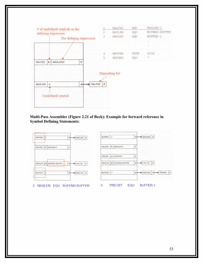
Multi-Pass Assembler (Figure 2.21 of Beck): Example for forward reference in Symbol Defining Statements:
53

54

Chapter 3
Loaders and Linkers
This Chapter gives you…
• Basic Loader Functions• Machine-Dependent Loader Features• Machine-Independent Loader Features• Loader Design Options• Implementation Examples
3.0 Introduction
The Source Program written in assembly language or high level language will be converted to object program, which is in the machine language form for execution. This conversion either from assembler or from compiler, contains translated instructions and data values from the source program, or specifies addresses in primary memory where these items are to be loaded for execution.
This contains the following three processes, and they are,
Loading - which allocates memory location and brings the object program into memory for execution - (Loader)
Linking- which combines two or more separate object programs and supplies the information needed to allow references between them - (Linker)
Relocation - which modifies the object program so that it can be loaded at an address different from the location originally specified - (Linking Loader)
3.1 Basic Loader Functions
A loader is a system program that performs the loading function. It brings object program into memory and starts its execution. The role of loader is as shown in the figure 3.1. In figure 3.1 translator may be assembler/complier, which generates the object program and later loaded to the memory by the loader for execution. In figure 3.2 the translator is specifically an assembler, which generates the object loaded, which becomes input to the loader. The figure 3.3 shows the role of both loader and linker.
55

Figure 3.1 : The Role of Loader
Figure 3.2: The Role of Loader with Assembler
TranslatorObject
Program Loader Object program ready for execution
Memory
AssemblerObject
Program Loader Object program ready for execution
Memory
56
SourceProgram
SourceProgram
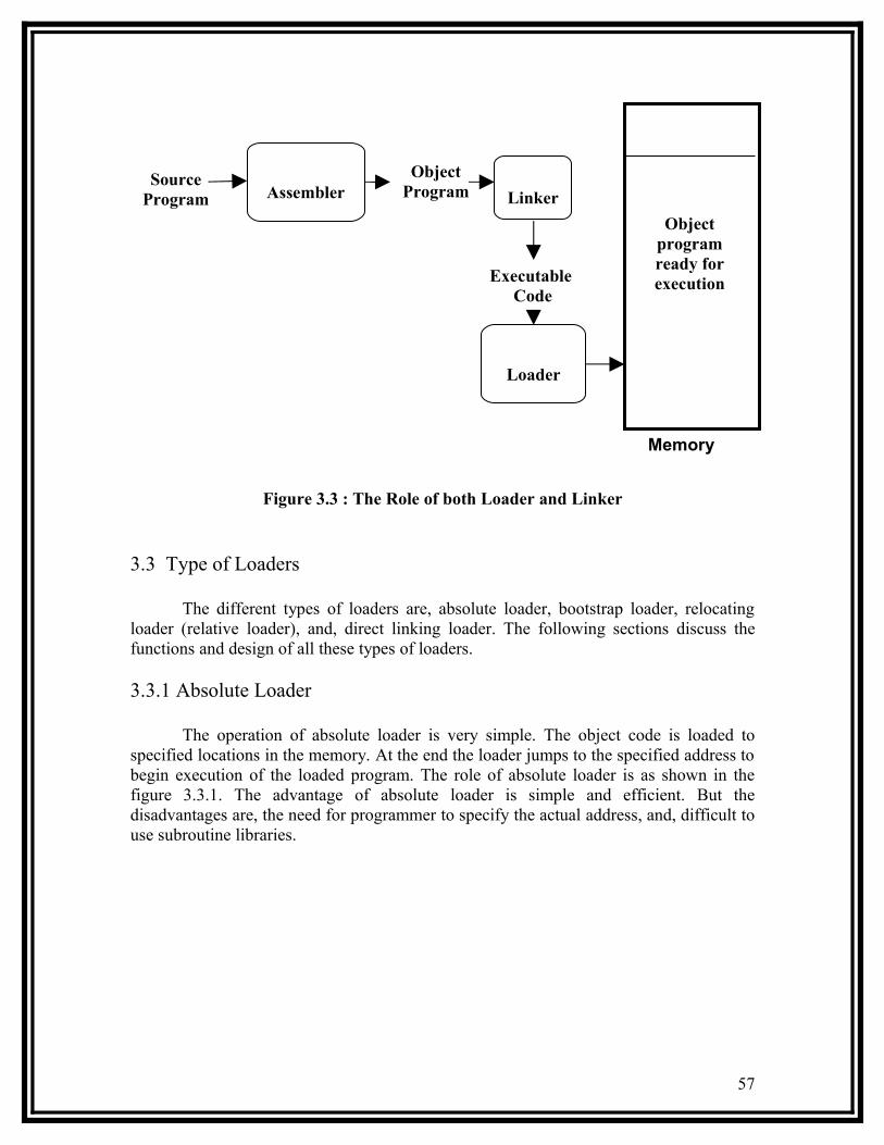
Figure 3.3 : The Role of both Loader and Linker
3.3 Type of Loaders
The different types of loaders are, absolute loader, bootstrap loader, relocating loader (relative loader), and, direct linking loader. The following sections discuss the functions and design of all these types of loaders.
3.3.1 Absolute Loader
The operation of absolute loader is very simple. The object code is loaded to specified locations in the memory. At the end the loader jumps to the specified address to begin execution of the loaded program. The role of absolute loader is as shown in the figure 3.3.1. The advantage of absolute loader is simple and efficient. But the disadvantages are, the need for programmer to specify the actual address, and, difficult to use subroutine libraries.
AssemblerObject
Program LinkerObject
program ready for execution
Memory
Executable Code
Loader
57
SourceProgram
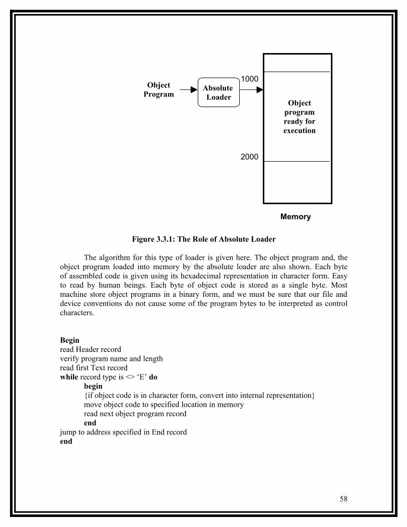
Figure 3.3.1: The Role of Absolute Loader
The algorithm for this type of loader is given here. The object program and, the object program loaded into memory by the absolute loader are also shown. Each byte of assembled code is given using its hexadecimal representation in character form. Easy to read by human beings. Each byte of object code is stored as a single byte. Most machine store object programs in a binary form, and we must be sure that our file and device conventions do not cause some of the program bytes to be interpreted as control characters.
Beginread Header recordverify program name and lengthread first Text recordwhile record type is <> ‘E’ do
begin{if object code is in character form, convert into internal representation}move object code to specified location in memoryread next object program recordend
jump to address specified in End recordend
ObjectProgram
Absolute Loader
Object program ready for execution
Memory
1000
2000
58

59
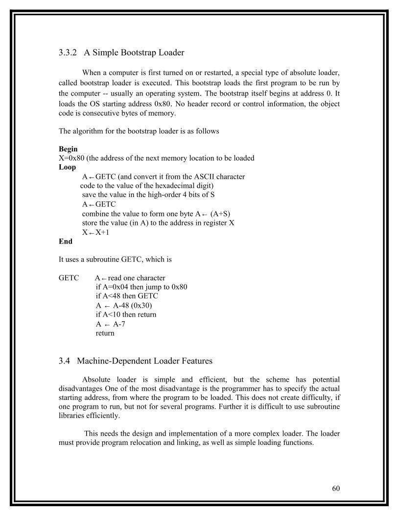
3.3.2 A Simple Bootstrap Loader
When a computer is first turned on or restarted, a special type of absolute loader, called bootstrap loader is executed. This bootstrap loads the first program to be run by the computer -- usually an operating system. The bootstrap itself begins at address 0. It loads the OS starting address 0x80. No header record or control information, the object code is consecutive bytes of memory.
The algorithm for the bootstrap loader is as follows
BeginX=0x80 (the address of the next memory location to be loaded Loop
A←GETC (and convert it from the ASCII character code to the value of the hexadecimal digit)
save the value in the high-order 4 bits of SA←GETC
combine the value to form one byte A← (A+S)store the value (in A) to the address in register XX←X+1
End
It uses a subroutine GETC, which is
GETC A←read one character if A=0x04 then jump to 0x80 if A<48 then GETC A ← A-48 (0x30) if A<10 then return A ← A-7 return
3.4 Machine-Dependent Loader Features
Absolute loader is simple and efficient, but the scheme has potential disadvantages One of the most disadvantage is the programmer has to specify the actual starting address, from where the program to be loaded. This does not create difficulty, if one program to run, but not for several programs. Further it is difficult to use subroutine libraries efficiently.
This needs the design and implementation of a more complex loader. The loader must provide program relocation and linking, as well as simple loading functions.
60
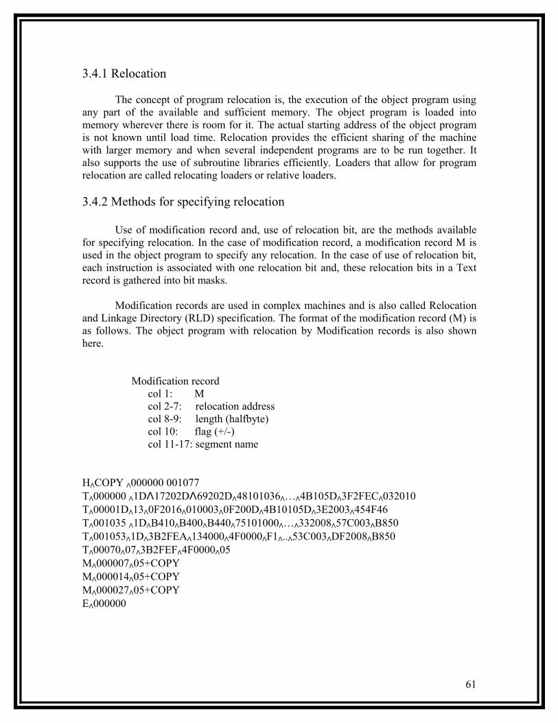
3.4.1 Relocation
The concept of program relocation is, the execution of the object program using any part of the available and sufficient memory. The object program is loaded into memory wherever there is room for it. The actual starting address of the object program is not known until load time. Relocation provides the efficient sharing of the machine with larger memory and when several independent programs are to be run together. It also supports the use of subroutine libraries efficiently. Loaders that allow for program relocation are called relocating loaders or relative loaders.
3.4.2 Methods for specifying relocation
Use of modification record and, use of relocation bit, are the methods available for specifying relocation. In the case of modification record, a modification record M is used in the object program to specify any relocation. In the case of use of relocation bit, each instruction is associated with one relocation bit and, these relocation bits in a Text record is gathered into bit masks.
Modification records are used in complex machines and is also called Relocation and Linkage Directory (RLD) specification. The format of the modification record (M) is as follows. The object program with relocation by Modification records is also shown here.
Modification recordcol 1: Mcol 2-7: relocation address col 8-9: length (halfbyte)col 10: flag (+/-)col 11-17: segment name
HΛCOPY Λ000000 001077TΛ000000 Λ1DΛ17202DΛ69202DΛ48101036Λ…Λ4B105DΛ3F2FECΛ032010TΛ00001DΛ13Λ0F2016Λ010003Λ0F200DΛ4B10105DΛ3E2003Λ454F46TΛ001035 Λ1DΛB410ΛB400ΛB440Λ75101000Λ…Λ332008Λ57C003ΛB850TΛ001053Λ1DΛ3B2FEAΛ134000Λ4F0000ΛF1Λ..Λ53C003ΛDF2008ΛB850TΛ00070Λ07Λ3B2FEFΛ4F0000Λ05MΛ000007Λ05+COPYMΛ000014Λ05+COPYMΛ000027Λ05+COPYEΛ000000
61

The relocation bit method is used for simple machines. Relocation bit is 0: no modification is necessary, and is 1: modification is needed. This is specified in the columns 10-12 of text record (T), the format of text record, along with relocation bits is as follows.
Text recordcol 1: Tcol 2-7: starting address col 8-9: length (byte)col 10-12: relocation bitscol 13-72: object code
Twelve-bit mask is used in each Text record (col:10-12 – relocation bits), since each text record contains less than 12 words, unused words are set to 0, and, any value that is to be modified during relocation must coincide with one of these 3-byte segments. For absolute loader, there are no relocation bits column 10-69 contains object code. The object program with relocation by bit mask is as shown below. Observe FFC - means all ten words are to be modified and, E00 - means first three records are to be modified.
HΛCOPY Λ000000 00107ATΛ000000Λ1EΛFFCΛ140033Λ481039Λ000036Λ280030Λ300015Λ…Λ3C0003 Λ …TΛ00001EΛ15ΛE00Λ0C0036Λ481061Λ080033Λ4C0000Λ…Λ000003Λ000000TΛ001039Λ1EΛFFCΛ040030Λ000030Λ…Λ30103FΛD8105DΛ280030Λ...TΛ001057Λ0AΛ 800Λ100036Λ4C0000ΛF1Λ001000TΛ001061Λ19ΛFE0Λ040030ΛE01079Λ…Λ508039ΛDC1079Λ2C0036Λ...EΛ000000
3.5 Program Linking
The Goal of program linking is to resolve the problems with external references (EXTREF) and external definitions (EXTDEF) from different control sections.
EXTDEF (external definition) - The EXTDEF statement in a control section names symbols, called external symbols, that are defined in this (present) control section and may be used by other sections.
ex: EXTDEF BUFFER, BUFFEND, LENGTH EXTDEF LISTA, ENDA
EXTREF (external reference) - The EXTREF statement names symbols used in this (present) control section and are defined elsewhere.
ex: EXTREF RDREC, WRREC EXTREF LISTB, ENDB, LISTC, ENDC
62
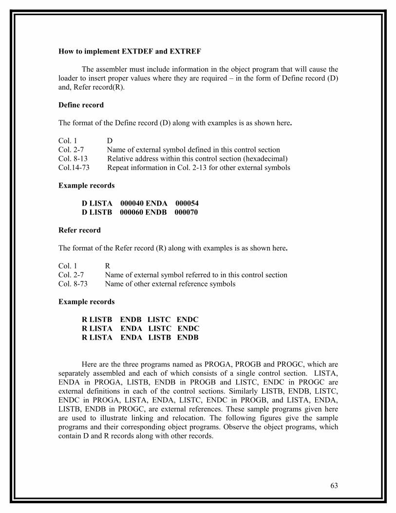
How to implement EXTDEF and EXTREF
The assembler must include information in the object program that will cause the loader to insert proper values where they are required – in the form of Define record (D) and, Refer record(R).
Define record
The format of the Define record (D) along with examples is as shown here.
Col. 1 DCol. 2-7 Name of external symbol defined in this control sectionCol. 8-13 Relative address within this control section (hexadecimal)Col.14-73 Repeat information in Col. 2-13 for other external symbols
Example records
D LISTA 000040 ENDA 000054 D LISTB 000060 ENDB 000070
Refer record
The format of the Refer record (R) along with examples is as shown here.
Col. 1 RCol. 2-7 Name of external symbol referred to in this control sectionCol. 8-73 Name of other external reference symbols
Example records
R LISTB ENDB LISTC ENDC R LISTA ENDA LISTC ENDC R LISTA ENDA LISTB ENDB
Here are the three programs named as PROGA, PROGB and PROGC, which are separately assembled and each of which consists of a single control section. LISTA, ENDA in PROGA, LISTB, ENDB in PROGB and LISTC, ENDC in PROGC are external definitions in each of the control sections. Similarly LISTB, ENDB, LISTC, ENDC in PROGA, LISTA, ENDA, LISTC, ENDC in PROGB, and LISTA, ENDA, LISTB, ENDB in PROGC, are external references. These sample programs given here are used to illustrate linking and relocation. The following figures give the sample programs and their corresponding object programs. Observe the object programs, which contain D and R records along with other records.
63

0000 PROGA START 0EXTDEF LISTA, ENDAEXTREF LISTB, ENDB, LISTC, ENDC………..……….
0020 REF1 LDA LISTA 03201D0023 REF2 +LDT LISTB+4 771000040027 REF3 LDX #ENDA-LISTA 050014
.
.0040 LISTA EQU *
0054 ENDA EQU *0054 REF4 WORD ENDA-LISTA+LISTC 0000140057 REF5 WORD ENDC-LISTC-10 FFFFF6005A REF6 WORD ENDC-LISTC+LISTA-1 00003F005D REF7 WORD ENDA-LISTA-(ENDB-LISTB) 0000140060 REF8 WORD LISTB-LISTA FFFFC0
END REF1
0000 PROGB START 0EXTDEF LISTB, ENDBEXTREF LISTA, ENDA, LISTC, ENDC………..……….
0036 REF1 +LDA LISTA 03100000003A REF2 LDT LISTB+4 772027003D REF3 +LDX #ENDA-LISTA 05100000
.
.0060 LISTB EQU *
0070 ENDB EQU *0070 REF4 WORD ENDA-LISTA+LISTC 0000000073 REF5 WORD ENDC-LISTC-10 FFFFF60076 REF6 WORD ENDC-LISTC+LISTA-1 FFFFFF0079 REF7 WORD ENDA-LISTA-(ENDB-LISTB) FFFFF0007C REF8 WORD LISTB-LISTA 000060
END
64

0000 PROGC START 0EXTDEF LISTC, ENDCEXTREF LISTA, ENDA, LISTB, ENDB………..………..
0018 REF1 +LDA LISTA 03100000001C REF2 +LDT LISTB+4 771000040020 REF3 +LDX #ENDA-LISTA 05100000
.
.0030 LISTC EQU *
0042 ENDC EQU *0042 REF4 WORD ENDA-LISTA+LISTC 0000300045 REF5 WORD ENDC-LISTC-10 0000080045 REF6 WORD ENDC-LISTC+LISTA-1 000011004B REF7 WORD ENDA-LISTA-(ENDB-LISTB) 000000004E REF8 WORD LISTB-LISTA 000000
END
H PROGA 000000 000063D LISTA 000040 ENDA 000054R LISTB ENDB LISTC ENDC..T 000020 0A 03201D 77100004 050014..T 000054 0F 000014 FFFF6 00003F 000014 FFFFC0M000024 05+LISTBM000054 06+LISTCM000057 06+ENDCM000057 06 -LISTCM00005A06+ENDCM00005A06 -LISTCM00005A06+PROGAM00005D06-ENDBM00005D06+LISTBM00006006+LISTBM00006006-PROGAE000020
65

H PROGB 000000 00007FD LISTB 000060 ENDB 000070R LISTA ENDA LISTC ENDC.T 000036 0B 03100000 772027 05100000.T 000007 0F 000000 FFFFF6 FFFFFF FFFFF0 000060M000037 05+LISTAM00003E 06+ENDAM00003E 06 -LISTAM000070 06 +ENDAM000070 06 -LISTAM000070 06 +LISTCM000073 06 +ENDCM000073 06 -LISTCM000073 06 +ENDCM000076 06 -LISTCM000076 06+LISTAM000079 06+ENDAM000079 06 -LISTAM00007C 06+PROGBM00007C 06-LISTAE
H PROGC 000000 000051D LISTC 000030 ENDC 000042R LISTA ENDA LISTB ENDB.T 000018 0C 03100000 77100004 05100000.T 000042 0F 000030 000008 000011 000000 000000 M000019 05+LISTAM00001D 06+LISTBM000021 06+ENDAM000021 06 -LISTAM000042 06+ENDAM000042 06 -LISTAM000042 06+PROGCM000048 06+LISTAM00004B 06+ENDAM00004B 006-LISTAM00004B 06-ENDBM00004B 06+LISTB M00004E 06+LISTBM00004E 06-LISTAE
66

The following figure shows these three programs as they might appear in memory after loading and linking. PROGA has been loaded starting at address 4000, with PROGB and PROGC immediately following.
67

For example, the value for REF4 in PROGA is located at address 4054 (the beginning address of PROGA plus 0054, the relative address of REF4 within PROGA). The following figure shows the details of how this value is computed.
The initial value from the Text record T0000540F000014FFFFF600003F000014FFFFC0 is 000014. To this is added the address assigned to LISTC, which is 4112 (the beginning address of PROGC plus 30). The result is 004126.
That is REF4 in PROGA is ENDA-LISTA+LISTC=4054-4040+4112=4126.
Similarly the load address for symbols LISTA: PROGA+0040=4040, LISTB: PROGB+0060=40C3 and LISTC: PROGC+0030=4112
Keeping these details work through the details of other references and values of these references are the same in each of the three programs.
68

3.6 Algorithm and Data structures for a Linking Loader
The algorithm for a linking loader is considerably more complicated than the absolute loader program, which is already given. The concept given in the program linking section is used for developing the algorithm for linking loader. The modification records are used for relocation so that the linking and relocation functions are performed using the same mechanism.
Linking Loader uses two-passes logic. ESTAB (external symbol table) is the main data structure for a linking loader.
Pass 1: Assign addresses to all external symbols Pass 2: Perform the actual loading, relocation, and linking
ESTAB - ESTAB for the example (refer three programs PROGA PROGB and PROGC) given is as shown below. The ESTAB has four entries in it; they are name of the control section, the symbol appearing in the control section, its address and length of the control section.
3.6.1 Program Logic for Pass 1
Pass 1 assign addresses to all external symbols. The variables & Data structures used during pass 1 are, PROGADDR (program load address) from OS, CSADDR (control section address), CSLTH (control section length) and ESTAB. The pass 1 processes the Define Record. The algorithm for Pass 1 of Linking Loader is given below.
69
Control section Symbol Address Length
PROGA 4000 63
LISTA 4040
ENDA 4054
PROGB 4063 7F
LISTB 40C3
ENDB 40D3
PROGC 40E2 51
LISTC 4112ENDC 4124

3.6.2 Program Logic for Pass 2
Pass 2 of linking loader perform the actual loading, relocation, and linking. It uses modification record and lookup the symbol in ESTAB to obtain its addres. Finally it uses end record of a main program to obtain transfer address, which is a starting address needed for the execution of the program. The pass 2 process Text record and Modification record of the object programs. The algorithm for Pass 2 of Linking Loader is given below.
70

3.6.3 Improve Efficiency, How?
The question here is can we improve the efficiency of the linking loader. Also observe that, even though we have defined Refer record (R), we haven’t made use of it. The efficiency can be improved by the use of local searching instead of multiple searches of ESTAB for the same symbol. For implementing this we assign a reference number to each external symbol in the Refer record. Then this reference number is used in Modification records instead of external symbols. 01 is assigned to control section name, and other numbers for external reference symbols.
The object programs for PROGA, PROGB and PROGC are shown below, with above modification to Refer record ( Observe R records).
71

72

Symbol and Addresses in PROGA, PROGB and PROGC are as shown below. These are the entries of ESTAB. The main advantage of reference number mechanism is that it avoids multiple searches of ESTAB for the same symbol during the loading of a control section
73
Ref No. Symbol Address
1 PROGA 4000
2 LISTB 40C3
3 ENDB 40D3
4 LISTC 4112
5 ENDC 4124
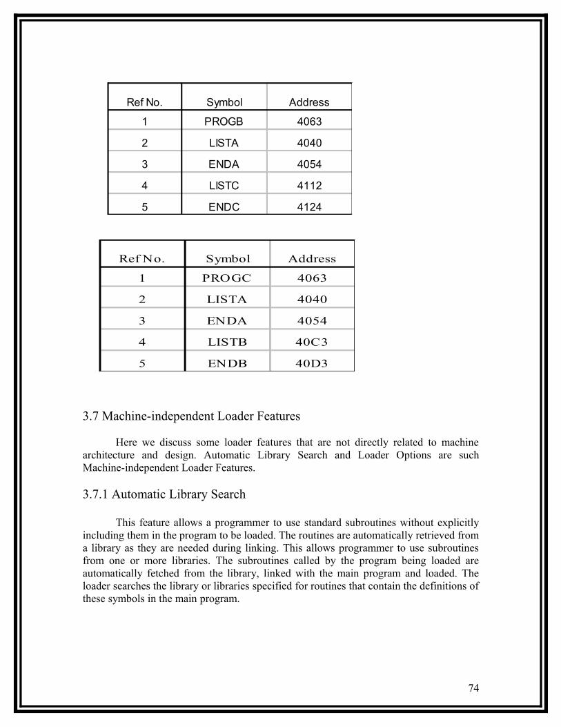
3.7 Machine-independent Loader Features
Here we discuss some loader features that are not directly related to machine architecture and design. Automatic Library Search and Loader Options are such Machine-independent Loader Features.
3.7.1 Automatic Library Search
This feature allows a programmer to use standard subroutines without explicitly including them in the program to be loaded. The routines are automatically retrieved from a library as they are needed during linking. This allows programmer to use subroutines from one or more libraries. The subroutines called by the program being loaded are automatically fetched from the library, linked with the main program and loaded. The loader searches the library or libraries specified for routines that contain the definitions of these symbols in the main program.
74
Ref No. Symbol Address
1 PROGB 4063
2 LISTA 4040
3 ENDA 4054
4 LISTC 4112
5 ENDC 4124
Ref No. Symbol Address
1 PROGC 4063
2 LISTA 4040
3 ENDA 4054
4 LISTB 40C3
5 ENDB 40D3
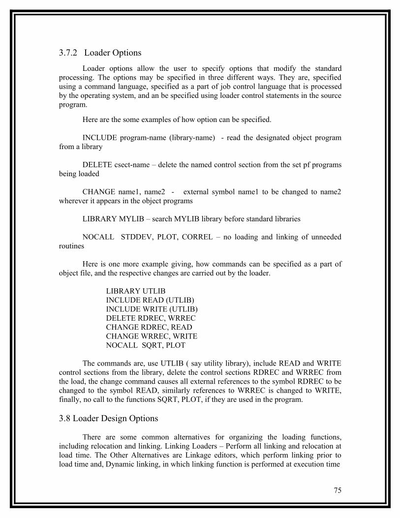
3.7.2 Loader Options
Loader options allow the user to specify options that modify the standard processing. The options may be specified in three different ways. They are, specified using a command language, specified as a part of job control language that is processed by the operating system, and an be specified using loader control statements in the source program.
Here are the some examples of how option can be specified.
INCLUDE program-name (library-name) - read the designated object program from a library
DELETE csect-name – delete the named control section from the set pf programs being loaded
CHANGE name1, name2 - external symbol name1 to be changed to name2 wherever it appears in the object programs
LIBRARY MYLIB – search MYLIB library before standard libraries
NOCALL STDDEV, PLOT, CORREL – no loading and linking of unneeded routines
Here is one more example giving, how commands can be specified as a part of object file, and the respective changes are carried out by the loader.
LIBRARY UTLIBINCLUDE READ (UTLIB)INCLUDE WRITE (UTLIB)DELETE RDREC, WRRECCHANGE RDREC, READCHANGE WRREC, WRITENOCALL SQRT, PLOT
The commands are, use UTLIB ( say utility library), include READ and WRITE control sections from the library, delete the control sections RDREC and WRREC from the load, the change command causes all external references to the symbol RDREC to be changed to the symbol READ, similarly references to WRREC is changed to WRITE, finally, no call to the functions SQRT, PLOT, if they are used in the program.
3.8 Loader Design Options
There are some common alternatives for organizing the loading functions, including relocation and linking. Linking Loaders – Perform all linking and relocation at load time. The Other Alternatives are Linkage editors, which perform linking prior to load time and, Dynamic linking, in which linking function is performed at execution time
75

3.8.1 Linking Loaders
The above diagram shows the processing of an object program using Linking Loader. The source program is first assembled or compiled, producing an object program. A linking loader performs all linking and loading operations, and loads the program into memory for execution.
3.8.2 Linkage Editors
The figure below shows the processing of an object program using Linkage editor. A linkage editor produces a linked version of the program – often called a load module or an executable image – which is written to a file or library for later execution. The linked program produced is generally in a form that is suitable for processing by a relocating loader.
Some useful functions of Linkage editor are, an absolute object program can be created, if starting address is already known. New versions of the library can be included without changing the source program. Linkage editors can also be used to build packages of subroutines or other control sections that are generally used together. Linkage editors often allow the user to specify that external references are not to be resolved by automatic library search – linking will be done later by linking loader – linkage editor + linking loader – savings in space
Library
Object Program(s)
Linking loader
Memory
76

3.8.3 Dynamic Linking
The scheme that postpones the linking functions until execution. A subroutine is loaded and linked to the rest of the program when it is first called – usually called dynamic linking, dynamic loading or load on call. The advantages of dynamic linking are, it allow several executing programs to share one copy of a subroutine or library. In an object oriented system, dynamic linking makes it possible for one object to be shared by several programs. Dynamic linking provides the ability to load the routines only when (and if) they are needed. The actual loading and linking can be accomplished using operating system service request.
Library
Object Program(s)
Linkage Editor
Linked program
Memory
Relocating loader
77

3.8.4 Bootstrap Loaders
If the question, how is the loader itself loaded into the memory ? is asked, then the answer is, when computer is started – with no program in memory, a program present in ROM ( absolute address) can be made executed – may be OS itself or A Bootstrap loader, which in turn loads OS and prepares it for execution. The first record ( or records) is generally referred to as a bootstrap loader – makes the OS to be loaded. Such a loader is added to the beginning of all object programs that are to be loaded into an empty and idle system.
3.9 Implementation Examples
This section contains brief description of loaders and linkers for actual computers. They are, MS-DOS Linker - Pentium architecture, SunOS Linkers - SPARC architecture, and, Cray MPP Linkers – T3E architecture.
3.9.1 MS-DOS Linker
This explains some of the features of Microsoft MS-DOS linker, which is a linker for Pentium and other x86 systems. Most MS-DOS compilers and assemblers (MASM) produce object modules, and they are stored in .OBJ files. MS-DOS LINK is a linkage editor that combines one or more object modules to produce a complete executable program - .EXE file; this file is later executed for results.
The following table illustrates the typical MS-DOS object module
Record Types Description
THEADR Translator HeaderTYPDEF,PUBDEF, EXTDEF External symbols and referencesLNAMES, SEGDEF, GRPDEF Segment definition and groupingLEDATA, LIDATA Translated instructions and dataFIXUPP Relocation and linking informationMODEND End of object module
THEADR specifies the name of the object module. MODEND specifies the end of the module. PUBDEF contains list of the external symbols (called public names). EXTDEF contains list of external symbols referred in this module, but defined elsewhere. TYPDEF the data types are defined here. SEGDEF describes segments in the object module ( includes name, length, and alignment). GRPDEF includes how segments are combined into groups. LNAMES contains all segment and class names. LEDATA contains translated instructions and data. LIDATA has above in repeating pattern. Finally, FIXUPP is used to resolve external references.
78
3.9.2 SunOS Linkers
SunOS Linkers are developed for SPARC systems. SunOS provides two different linkers – link-editor and run-time linker.
Link-editor is invoked in the process of assembling or compiling a program – produces a single output module – one of the following types
A relocatable object module – suitable for further link-editing
A static executable – with all symbolic references bound and ready to run
A dynamic executable – in which some symbolic references may need to be bound at run time
A shared object – which provides services that can be, bound at run time to one ore more dynamic executables
An object module contains one or more sections – representing instructions and data area from the source program, relocation and linking information, external symbol table.
Run-time linker uses dynamic linking approach. Run-time linker binds dynamic executables and shared objects at execution time. Performs relocation and linking operations to prepare the program for execution.
3.9.3 Cray MPP Linker
Cray MPP (massively parallel processing) Linker is developed for Cray T3E systems. A T3E system contains large number of parallel processing elements (PEs) – Each PE has local memory and has access to remote memory (memory of other PEs). The processing is divided among PEs - contains shared data and private data. The loaded program gets copy of the executable code, its private data and its portion of the shared data. The MPP linker organizes blocks containing executable code, private data and shared data. The linker then writes an executable file that contains the relocated and linked blocks. The executable file also specifies the number of PEs required and other control information. The linker can create an executable file that is targeted for a fixed number of PEs, or one that allows the partition size to be chosen at run time. Latter type is called plastic executable.
___________________
79

Chapter 4
Macro Processor
A Macro represents a commonly used group of statements in the source programming language.
• A macro instruction (macro) is a notational convenience for the programmero It allows the programmer to write shorthand version of a program (module
programming)• The macro processor replaces each macro instruction with the corresponding
group of source language statements (expanding)o Normally, it performs no analysis of the text it handles.o It does not concern the meaning of the involved statements during macro
expansion.• The design of a macro processor generally is machine independent!• Two new assembler directives are used in macro definition
o MACRO: identify the beginning of a macro definitiono MEND: identify the end of a macro definition
• Prototype for the macroo Each parameter begins with ‘&’
name MACRO parameters:body:
MENDo Body: the statements that will be generated as the expansion of the macro.
4.1 Basic Macro Processor Functions:
• Macro Definition and Expansion• Macro Processor Algorithms and Data structures
4.1.1 Macro Definition and Expansion:
The figure shows the MACRO expansion. The left block shows the MACRO definition and the right block shows the expanded macro replacing the MACRO call with its block of executable instruction.
M1 is a macro with two parameters D1 and D2. The MACRO stores the contents of register A in D1 and the contents of register B in D2. Later M1 is invoked with the parameters DATA1 and DATA2, Second time with DATA4 and DATA3. Every call of MACRO is expended with the executable statements.
80
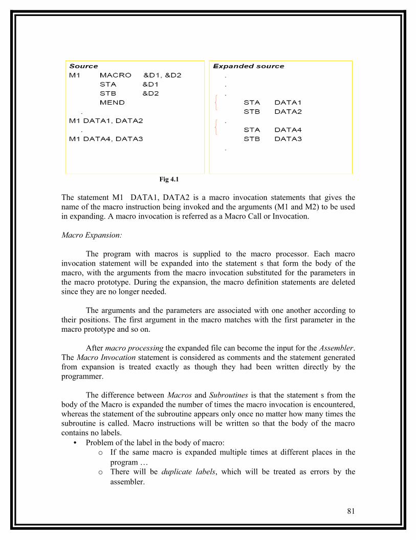
Fig 4.1
The statement M1 DATA1, DATA2 is a macro invocation statements that gives the name of the macro instruction being invoked and the arguments (M1 and M2) to be used in expanding. A macro invocation is referred as a Macro Call or Invocation.
Macro Expansion:
The program with macros is supplied to the macro processor. Each macro invocation statement will be expanded into the statement s that form the body of the macro, with the arguments from the macro invocation substituted for the parameters in the macro prototype. During the expansion, the macro definition statements are deleted since they are no longer needed.
The arguments and the parameters are associated with one another according to their positions. The first argument in the macro matches with the first parameter in the macro prototype and so on.
After macro processing the expanded file can become the input for the Assembler. The Macro Invocation statement is considered as comments and the statement generated from expansion is treated exactly as though they had been written directly by the programmer.
The difference between Macros and Subroutines is that the statement s from the body of the Macro is expanded the number of times the macro invocation is encountered, whereas the statement of the subroutine appears only once no matter how many times the subroutine is called. Macro instructions will be written so that the body of the macro contains no labels.
• Problem of the label in the body of macro:o If the same macro is expanded multiple times at different places in the
program …o There will be duplicate labels, which will be treated as errors by the
assembler.
81

• Solutions:o Do not use labels in the body of macro.o Explicitly use PC-relative addressing instead.
• Ex, in RDBUFF and WRBUFF macros,o JEQ *+11o JLT *-14
• It is inconvenient and error-prone.
The following program shows the concept of Macro Invocation and Macro Expansion.
82

Fig 4.2
4.1.2 Macro Processor Algorithm and Data Structure:
Design can be done as two-pass or a one-pass macro. In case of two-pass assembler.
Two-pass macro processor• You may design a two-pass macro processor
o Pass 1: Process all macro definitions
o Pass 2: Expand all macro invocation statements
• However, one-pass may be enougho Because all macros would have to be defined during the first pass before
any macro invocations were expanded. The definition of a macro must appear before any statements that
invoke that macro.• Moreover, the body of one macro can contain definitions of the other macro• Consider the example of a Macro defining another Macro.• In the example below, the body of the first Macro (MACROS) contains statement
that define RDBUFF, WRBUFF and other macro instructions for SIC machine.• The body of the second Macro (MACROX) defines the se same macros for
SIC/XE machine. • A proper invocation would make the same program to perform macro invocation
to run on either SIC or SIC/XEmachine.
83

MACROS for SIC machine
Fig 4.3(a)
MACROX for SIC/XE Machine
Fig 4.3(b)
• A program that is to be run on SIC system could invoke MACROS whereas a program to be run on SIC/XE can invoke MACROX.
• However, defining MACROS or MACROX does not define RDBUFF and WRBUFF.
• These definitions are processed only when an invocation of MACROS or MACROX is expanded.
84

One-Pass Macro Processor:• A one-pass macro processor that alternate between macro definition and macro
expansion in a recursive way is able to handle recursive macro definition.• Restriction
o The definition of a macro must appear in the source program before any statements that invoke that macro.
o This restriction does not create any real inconvenience.
The design considered is for one-pass assembler. The data structures required are:• DEFTAB (Definition Table)
Stores the macro definition including macro prototype and macro bodyComment lines are omitted.
o References to the macro instruction parameters are converted to a positional notation for efficiency in substituting arguments.
• NAMTAB (Name Table)Stores macro namesServes as an index to DEFTAB
Pointers to the beginning and the end of the macro definition (DEFTAB)
• ARGTAB (Argument Table)
Stores the arguments according to their positions in the argument list.
o As the macro is expanded the arguments from the Argument table are substituted for the corresponding parameters in the macro body. o The figure below shows the different data structures described and their relationship.
85

Fig 4.4
The above figure shows the portion of the contents of the table during the processing of the program in page no. 3. In fig 4.4(a) definition of RDBUFF is stored in DEFTAB, with an entry in NAMTAB having the pointers to the beginning and the end of the definition. The arguments referred by the instructions are denoted by the their positional notations. For example,
TD =X’?1’The above instruction is to test the availability of the device whose number is given by the parameter &INDEV. In the instruction this is replaced by its positional value? 1. Figure 4.4(b) shows the ARTAB as it would appear during expansion of the RDBUFF statement as given below:
CLOOP RDBUFF F1, BUFFER, LENGTHFor the invocation of the macro RDBUFF, the first parameter is F1 (input device code), second is BUFFER (indicating the address where the characters read are stored), and the third is LENGTH (which indicates total length of the record to be read). When the ?n notation is encountered in a line fro DEFTAB, a simple indexing operation supplies the proper argument from ARGTAB.
The algorithm of the Macro processor is given below. This has the procedure DEFINE to make the entry of macro name in the NAMTAB, Macro Prototype in DEFTAB. EXPAND is called to set up the argument values in ARGTAB and expand a Macro Invocation statement. Procedure GETLINE is called to get the next line to be processed either from the DEFTAB or from the file itself.
When a macro definition is encountered it is entered in the DEFTAB. The normal approach is to continue entering till MEND is encountered. If there is a program having a Macro defined within another Macro. While defining in the DEFTAB the very first MEND is taken as the end of the Macro definition. This does not complete the definition as there is another outer Macro which completes the difintion of Macro as a whole. Therefore the DEFINE procedure keeps a counter variable LEVEL. Every time a Macro directive is encountered this counter is incremented by 1. The moment the innermost Macro ends indicated by the directive MEND it starts decreasing the value of the counter variable by one. The last MEND should make the counter value set to zero. So when LEVEL becomes zero, the MEND corresponds to the original MACRO directive.
Most macro processors allow thr definitions of the commonly used instructions to appear in a standard system library, rather than in the source program. This makes the use of macros convenient; definitions are retrieved from the library as they are needed during macro processing.
86

Fig 4.5
87

Algorithms
88

Fig 4.6
4.1.3 Comparison of Macro Processor Design
• One-pass algorithmo Every macro must be defined before it is calledo One-pass processor can alternate between macro definition and macro
expansiono Nested macro definitions are allowed but nested calls are not allowed.
• Two-pass algorithmo Pass1: Recognize macro definitionso Pass2: Recognize macro callso Nested macro definitions are not allowed
89

4.1 Machine-independent Macro-Processor Features.
The design of macro processor doesn’t depend on the architecture of the machine. We will be studying some extended feature for this macro processor. These features are:
• Concatenation of Macro Parameters• Generation of unique labels• Conditional Macro Expansion• Keyword Macro Parameters
4.2.1 Concatenation of unique labels:
Most macro processor allows parameters to be concatenated with other character strings. Suppose that a program contains a series of variables named by the symbols XA1, XA2, XA3,…, another series of variables named XB1, XB2, XB3,…, etc. If similar processing is to be performed on each series of labels, the programmer might put this as a macro instruction. The parameter to such a macro instruction could specify the series of variables to be operated on (A, B, etc.). The macro processor would use this parameter to construct the symbols required in the macro expansion (XA1, Xb1, etc.).
Suppose that the parameter to such a macro instruction is named &ID. The body of the macro definition might contain a statement like
LDA X&ID1
Fig 4.7
& is the starting character of the macro instruction; but the end of the parameter is not marked. So in the case of &ID1, the macro processor could deduce the meaning that was intended. If the macro definition contains contain &ID and &ID1 as parameters, the situation would be unavoidably ambiguous.
Most of the macro processors deal with this problem by providing a special concatenation operator. In the SIC macro language, this operator is the character →. Thus the statement LDA X&ID1 can be written as
LDA X&ID→
90

Fig 4.8 The above figure shows a macro definition that uses the concatenation operator as
previously described. The statement SUM A and SUM BETA shows the invocation statements and the corresponding macro expansion.
4.2.2 Generation of Unique Labels
As discussed it is not possible to use labels for the instructions in the macro definition, since every expansion of macro would include the label repeatedly which is not allowed by the assembler. This in turn forces us to use relative addressing in the jump instructions. Instead we can use the technique of generating unique labels for every macro invocation and expansion. During macro expansion each $ will be replaced with $XX, where xx is a two-character alphanumeric counter of the number of macro instructions expansion.
For example, XX = AA, AB, AC…
This allows 1296 macro expansions in a single program.
91
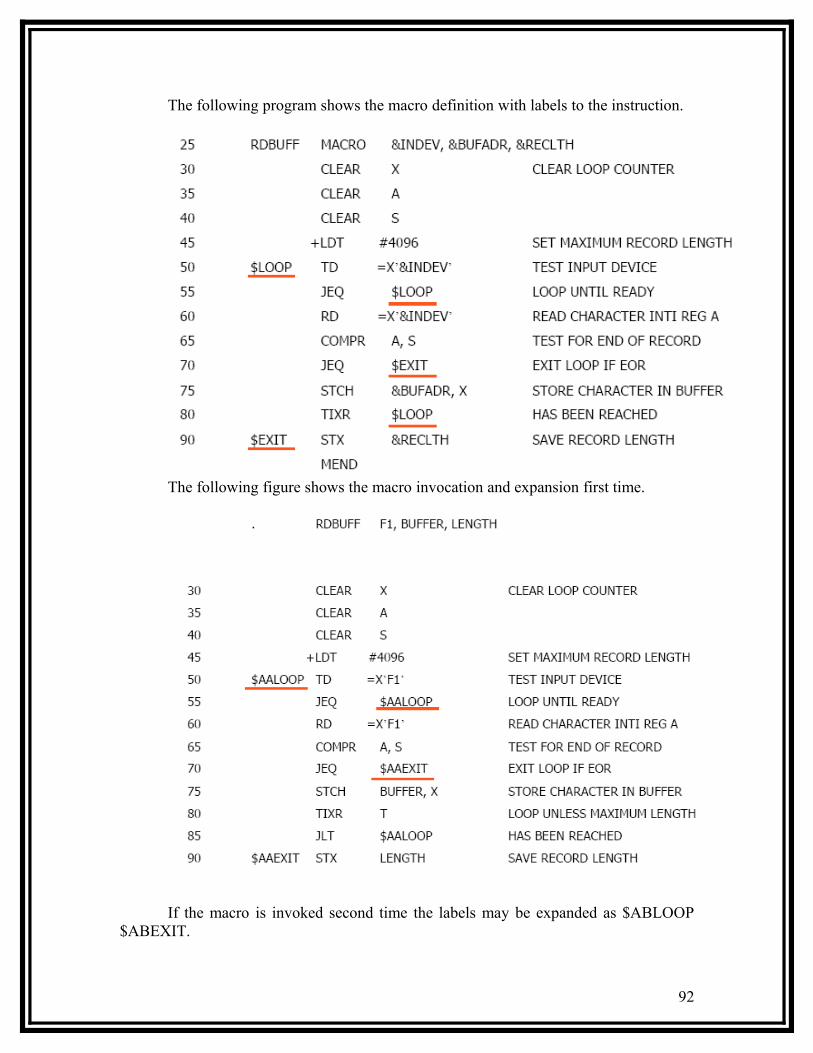
The following program shows the macro definition with labels to the instruction.
The following figure shows the macro invocation and expansion first time.
If the macro is invoked second time the labels may be expanded as $ABLOOP $ABEXIT.
92
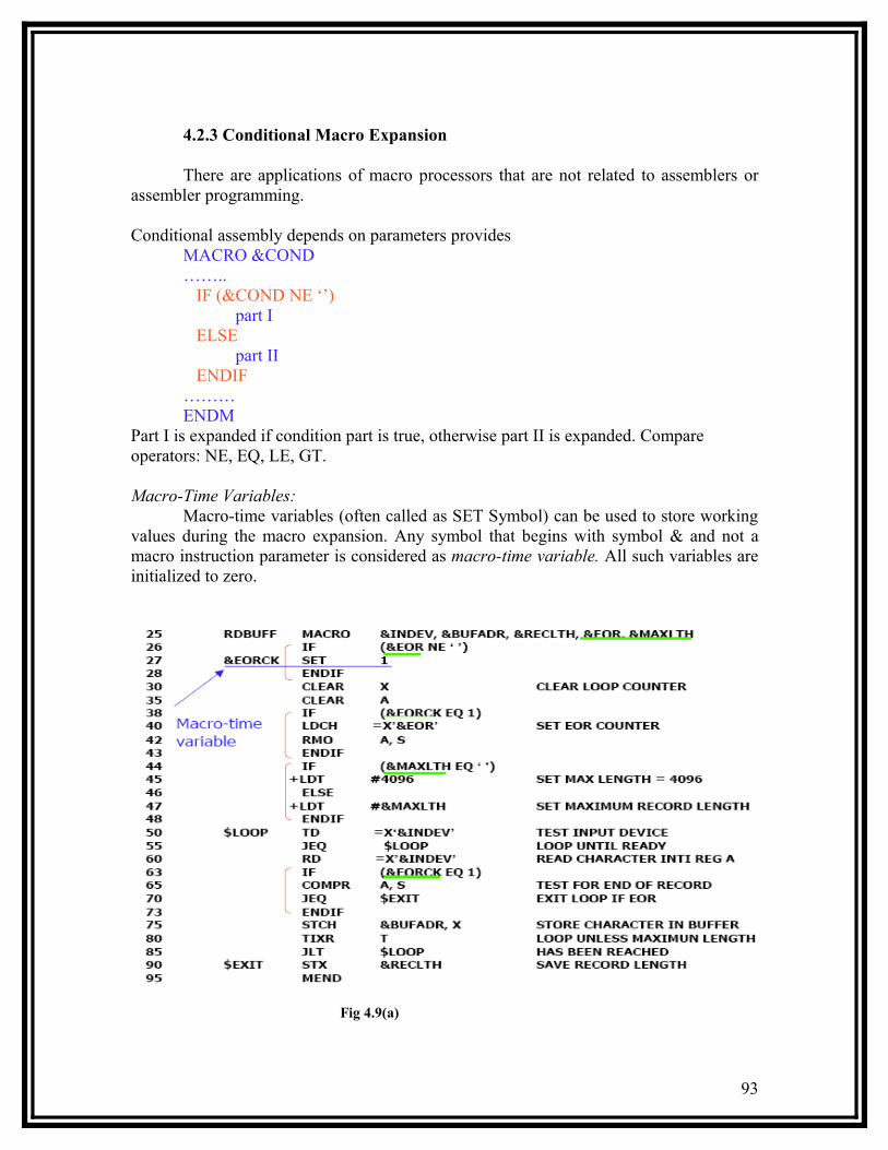
4.2.3 Conditional Macro Expansion
There are applications of macro processors that are not related to assemblers or assembler programming.
Conditional assembly depends on parameters providesMACRO &COND…….. IF (&COND NE ‘’)
part I ELSE
part II ENDIF………ENDM
Part I is expanded if condition part is true, otherwise part II is expanded. Compare operators: NE, EQ, LE, GT.
Macro-Time Variables:Macro-time variables (often called as SET Symbol) can be used to store working
values during the macro expansion. Any symbol that begins with symbol & and not a macro instruction parameter is considered as macro-time variable. All such variables are initialized to zero.
Fig 4.9(a)
93

Figure 4.5(a) gives the definition of the macro RDBUFF with the parameters &INDEV, &BUFADR, &RECLTH, &EOR, &MAXLTH. According to the above program if &EOR has any value, then &EORCK is set to 1 by using the directive SET, otherwise it retains its default value 0.
Fig 4.9(b) Use of Macro-Time Variable with EOF being NOT NULL
Fig 4.9(c) Use of Macro-Time conditional statement with EOF being NULL
94
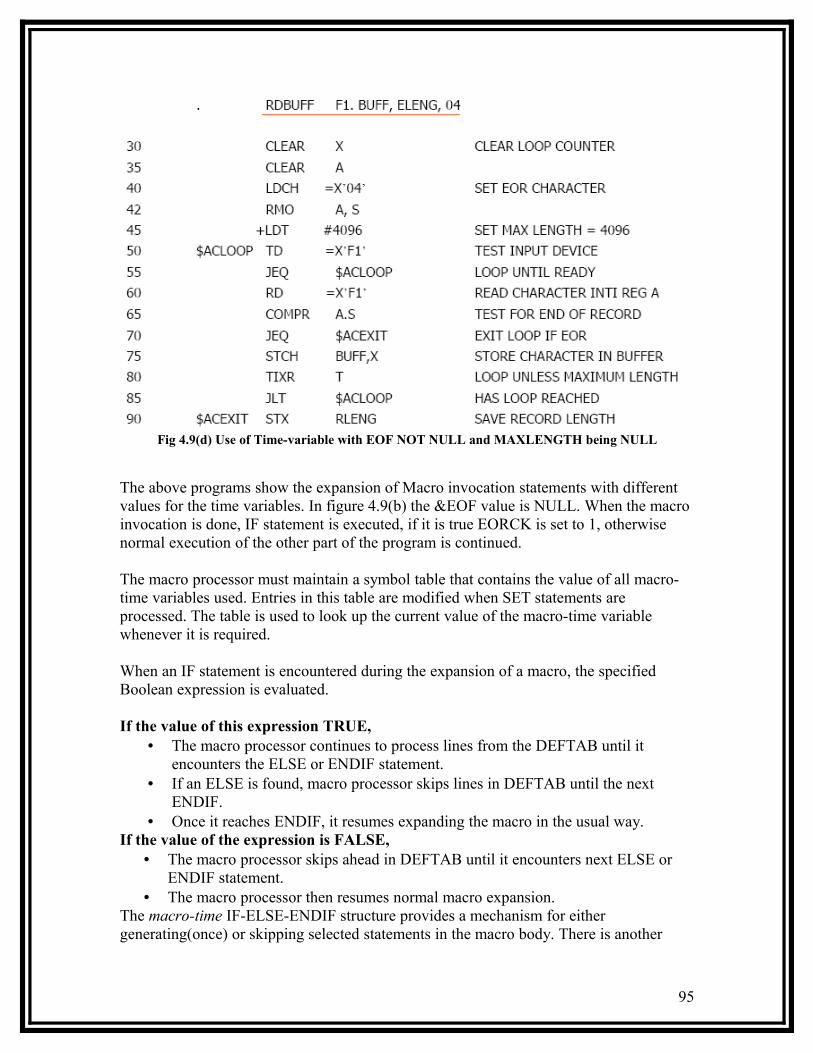
Fig 4.9(d) Use of Time-variable with EOF NOT NULL and MAXLENGTH being NULL
The above programs show the expansion of Macro invocation statements with different values for the time variables. In figure 4.9(b) the &EOF value is NULL. When the macro invocation is done, IF statement is executed, if it is true EORCK is set to 1, otherwise normal execution of the other part of the program is continued.
The macro processor must maintain a symbol table that contains the value of all macro-time variables used. Entries in this table are modified when SET statements are processed. The table is used to look up the current value of the macro-time variable whenever it is required.
When an IF statement is encountered during the expansion of a macro, the specified Boolean expression is evaluated.
If the value of this expression TRUE,• The macro processor continues to process lines from the DEFTAB until it
encounters the ELSE or ENDIF statement.• If an ELSE is found, macro processor skips lines in DEFTAB until the next
ENDIF.• Once it reaches ENDIF, it resumes expanding the macro in the usual way.
If the value of the expression is FALSE,• The macro processor skips ahead in DEFTAB until it encounters next ELSE or
ENDIF statement.• The macro processor then resumes normal macro expansion.
The macro-time IF-ELSE-ENDIF structure provides a mechanism for either generating(once) or skipping selected statements in the macro body. There is another
95

construct WHILE statement which specifies that the following line until the next ENDW statement, are to be generated repeatedly as long as a particular condition is true. The testing of this condition, and the looping are done during the macro is under expansion. The example shown below shows the usage of Macro-Time Looping statement.
WHILE-ENDW structure• When an WHILE statement is encountered during the expansion of a macro, the
specified Boolean expression is evaluated.• TRUE
o The macro processor continues to process lines from DEFTAB until it encounters the next ENDW statement.
o When ENDW is encountered, the macro processor returns to the preceding WHILE, re-evaluates the Boolean expression, and takes action based on the new value.
• FALSEo The macro processor skips ahead in DEFTAB until it finds the next
ENDW statement and then resumes normal macro expansion.
96

4.2.4 Keyword Macro Parameters
All the macro instruction definitions used positional parameters. Parameters and arguments are matched according to their positions in the macro prototype and the macro invocation statement. The programmer needs to be careful while specifying the arguments. If an argument is to be omitted the macro invocation statement must contain a null argument mentioned with two commas.
Positional parameters are suitable for the macro invocation. But if the macro invocation has large number of parameters, and if only few of the values need to be used in a typical invocation, a different type of parameter specification is required (for example, in many cases most of the parameters may have default values, and the invocation may mention only the changes from the default values).
Ex: XXX MACRO &P1, &P2, …., &P20, ….XXX A1, A2,,,,,,,,,,…,,A20,…..
Null arguments
Keyword parameters• Each argument value is written with a keyword that names the corresponding
parameter.• Arguments may appear in any order.• Null arguments no longer need to be used.• Ex: XXX P1=A1, P2=A2, P20=A20.• It is easier to read and much less error-prone than the positional method.
97
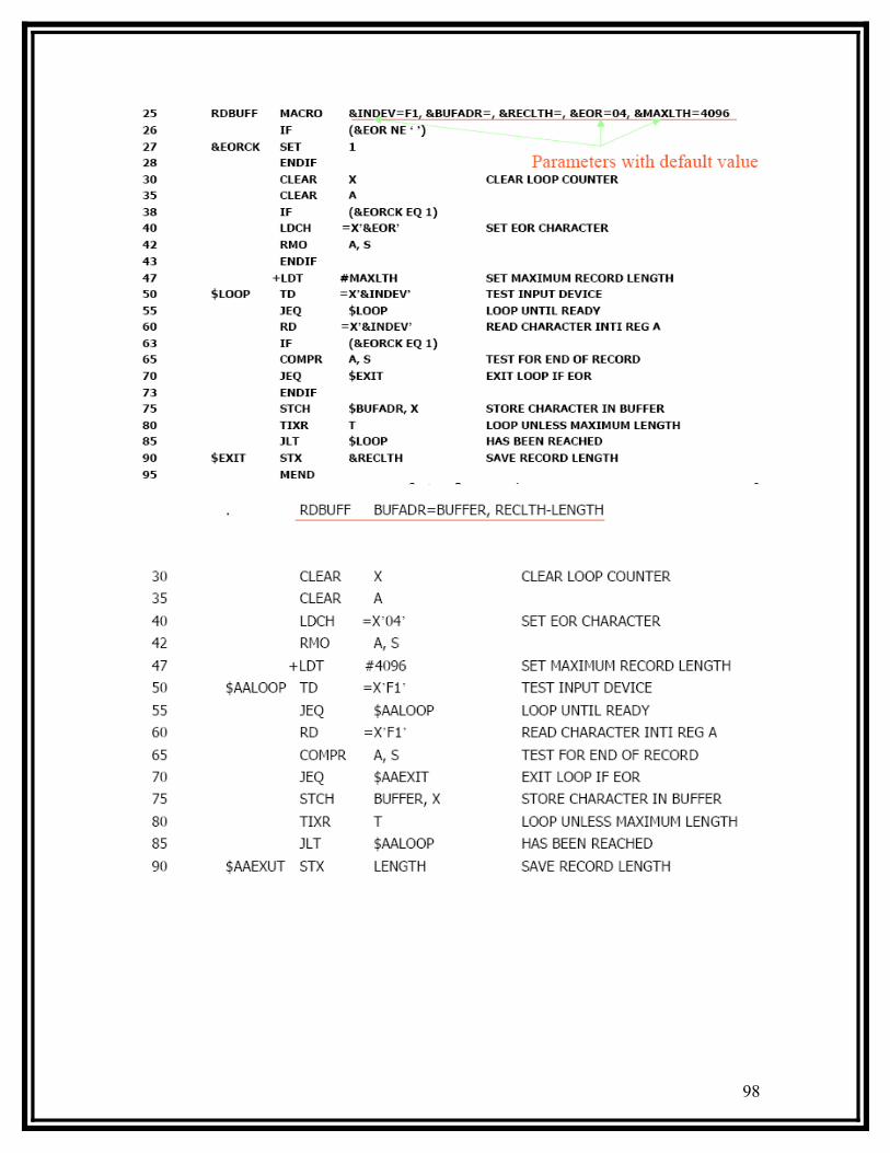
98

Fig 4.10 Example showing the usage of Keyword Parameter
4.3 Macro Processor Design Options
4.3.1 Recursive Macro Expansion
We have seen an example of the definition of one macro instruction by another. But we have not dealt with the invocation of one macro by another. The following example shows the invocation of one macro by another macro.
99

Problem of Recursive Expansion
• Previous macro processor design cannot handle such kind of recursive macro invocation and expansion
o The procedure EXPAND would be called recursively, thus the invocation arguments in the ARGTAB will be overwritten. (P.201)
o The Boolean variable EXPANDING would be set to FALSE when the “inner” macro expansion is finished, i.e., the macro process would forget that it had been in the middle of expanding an “outer” macro.
• Solutionso Write the macro processor in a programming language that allows
recursive calls, thus local variables will be retained.o If you are writing in a language without recursion support, use a stack to
take care of pushing and popping local variables and return addresses.
100

The procedure EXPAND would be called when the macro was recognized. The arguments from the macro invocation would be entered into ARGTAB as follows:
Parameter Value1 BUFFER2 LENGTH3 F14 (unused)- -
The Boolean variable EXPANDING would be set to TRUE, and expansion of the macro invocation statement would begin. The processing would proceed normally until statement invoking RDCHAR is processed. This time, ARGTAB would look like
Parameter Value1 F12 (Unused)-- --
At the expansion, when the end of RDCHAR is recognized, EXPANDING would be set to FALSE. Thus the macro processor would ‘forget’ that it had been in the middle of expanding a macro when it encountered the RDCHAR statement. In addition, the arguments from the original macro invocation (RDBUFF) would be lost because the value in ARGTAB was overwritten with the arguments from the invocation of RDCHAR.
4.3.2 General-Purpose Macro Processors
• Macro processors that do not dependent on any particular programming language, but can be used with a variety of different languages
• Proso Programmers do not need to learn many macro languages.o Although its development costs are somewhat greater than those for a
language specific macro processor, this expense does not need to be repeated for each language, thus save substantial overall cost.
• Conso Large number of details must be dealt with in a real programming
language Situations in which normal macro parameter substitution should
not occur, e.g., comments. Facilities for grouping together terms, expressions, or statements Tokens, e.g., identifiers, constants, operators, keywords Syntax had better be consistent with the source programming
language
101

4.3.3 Macro Processing within Language Translators
The macro processors we discussed are called “Preprocessors”.
o Process macro definitionso Expand macro invocationso Produce an expanded version of the source program, which is then used as input to an assembler or compiler
• You may also combine the macro processing functions with the language translator:
Line-by-line macro processorIntegrated macro processor
4.3.4 Line-by-Line Macro Processor
Used as a sort of input routine for the assembler or compilerRead source programProcess macro definitions and expand macro invocationsPass output lines to the assembler or compiler
Benefitso Avoid making an extra pass over the source program.o Data structures required by the macro processor and the language translator can be combined (e.g., OPTAB and NAMTAB)o Utility subroutines can be used by both macro processor and the language translator.
Scanning input linesSearching tablesData format conversionIt is easier to give diagnostic messages related to the source statements
4.3.5 Integrated Macro Processor
• An integrated macro processor can potentially make use of any information about the source program that is extracted by the language translator.
o Ex (blanks are not significant in FORTRAN) DO 100 I = 1,20
• a DO statement DO 100 I = 1
• An assignment statement• DO100I: variable (blanks are not significant in FORTRAN)
102

• An integrated macro processor can support macro instructions that depend upon the context in which they occur.
103

CHAPTER-5 COMPILERS
BASIC COMPILER FUNCTIONS
A compiler accepts a program written in a high level language as input and produces its machine language equivalent as output. For the purpose of compiler construction, a high level programming language is described in terms of a grammar. This grammar specifies the formal description of the syntax or legal statements in thelanguage.
Example: Assignment statement in Pascal is defined as:
< variable > : = < Expression >
The compiler has to match statement written by the programmer to the structure defined by the grammars and generates appropriate object code for each statement. The compilation process is so complex that it is not reasonable to implement it in one single step. It is partitioned into a series of sub-process called phases. A phase is a logically cohesive operation that takes as input one representation of the source program and produces an output of another representation. The basic phases are - Lexical Analysis, Syntax Analysis, and Code Generation.
Lexical Analysis: It is the first phase. It is also called scanner. It separates characters of the source language into groups that logically belong together. These groups are called tokens. The usual tokens are:
Keyword: such as DO or IF, Identifiers: such as x or num,
Operator symbols: such as <, =, or, +, and Punctuation symbols: such as parentheses or commas.
The output of the lexical analysis is a stream of tokens, which is passed to thenext phase; the syntax analyzer or parser.
Syntax Analyzer: It groups tokens together into syntactic structure. For example, the three tokens representing A + B might be grouped into a syntactic structure called as expression. Expressions might further be combined to form statements. Often the syntactic structures can be regarded as a tree whose leaves are the tokens. The interior nodes of the tree represent strings of token that logically belong together. Fig. 1 shows the syntax tree for READ statement in PASCAL (read)
(id - list)
READ ( id ) {value}
Fig. 1 Syntax Tree
Code Generator: It produces the object code by deciding on the memory locations for data, selecting code to access each datum and selecting the registers in which each computation is
104

to be done. Designing a code generator that produces truly efficient object program is one of the most difficult parts of compiler design.
In the following sections we discuss the basic elements of a simple compilation process, illustrating this application to the example program in fig. 2.
PROGRAM STATSVAR
SUM, SUMSQ, I, VALUE, MEAN, VARIANCE : INTEGERBEGIN
SUM : = 0 ;SUMSQ : = 0 ;FOR I : = 1 to 100 Do
BEGINREAD (VALUE) ;SUM : = SUM + VALUE ;SUMSQ : = SUMSQ + VALUE * VALUE
END;MEAN : = SUM DIV 100;VARIANCE : = SUMSQ DIV 100 - MEAN * MEAN ;WRITE (MEAN, VARIANCE)
ENDFig. 2 Pascal Program
GRAMMARSA grammar for a programming language is a formal description of the syntax of programs
and individual statements written in the language. The grammar does not describe the semantics or memory of the various statements. To differentiate between syntax and semantics consider the following example:
VAR X, Y : REAL VAR I, J, K : INTEGER I : INTEGER X : = I + Y ; I : = J + K ;
Fig .3 These two programs statement have identical syntax. Each is an assignment statement; the value to be assigned is given by an expression that consists of two variable names separated by the operator '+'.
The semantics of the two statements are quite different. The first statement specifies that the variables in the expressions are to be added using integer arithmetic operations. The second statement specifies a floating-point addition, with the integer operand 2 being connected to floating point before adding. The difference between the statements would be recognized during code generation.
Grammar can be written using a number of different notations. Backus-Naur Form (BNF) is one of the methods available. It is simple and widely used. It provides capabilities that are different for most purposes.
A BNF grammar consists of a set of rules, each of which defines the syntax of some construct in the programming language.
A grammar has four components. They are:
105

1. A set of tokens, known as terminal symbols non-enclosed in bracket. Example:
READ, WRITE
2. A set of terminals. The character strings enclosed between the angle brackets (<, >) are called terminal symbols. These are the names of the constructs defined in the grammar.
3. A set of productions where each production consists of a non-terminal called the left side of the production, as "is defined to be" (:: = ), and a sequence of
token and/or non-terminal, called the right side of the product.
Example: < reads > : : = READ <id - list >.
4. A designation of one of the non-terminals as the start symbol.
This rule offers two possibilities separated by the symbol, for the syntax of an < id - list > may consist simply of a token id (the notation id denotes an identifier that is recognized by the scanner). The second syntax.
Example: ALPHAALPHA, BETA
ALPHA is an < id - list > that consist of another < id - list > ALPHA, followedby a comma, followed by an id BETA.
Tree: It is also called parse tree or syntax tree. It is convenient to display the analysis of a source statement in terms of a grammar as a tree.
Example: READ (VALUE)GRAMMAR: (read) : : = READ ( < id -list>)
Example: Assignment statement:
SUM : = 0 ;SUM : = + VALUE ;SUM : = - VALUE ;
Grammar: < assign > : : = id : = < exp > < exp > : : = < term > | < exp > - < term > < term > : : = < factor > | < term > * < factor > | < term > DIV < factor > < factor > : : = id | int | ( < exp > )
Assign consists of an id followed by the token : = , followed by an expression <exp > Fig. 4(a). Show the syntax tree.
Expressions are sequence of <terms> connected by the operations + and - Fig. 4(b). Show the syntax tree.
Term is a sequence of < factor > S connected by * and DIV Fig. 4(c).
A factor may consists of an identifies id or an int (which is also recognized by the scan) or an < exp > enclosed in parenthesis. Fig. 4(d).
< assign > < exp >
id : = <exp > < term > + < exp > {variance }
106

Fig. 4 (a) Fig. 4 (b)
< term > factor | |
< factor > Dir < term > id
X < factor > int
IdFig.4 (c)
(< exp > ) Fig. 4 (d)
Fig. 4 Parse Trees
For the statement Variance : = SUMSQ Div 100 - MEAN * MEAN ;The list of simplified Pascal grammar is shown in fig.5.
1. < prog > : : = PROGRAM < program > VAR <dec - list > BEGIN < stmt > - list > END.
2. < prog - name >: : = id3. < dec - list > : : = < dec > | < dec - list > ; < dec >4. < dec > : : = < id - list > : < type >5. < type > : : = integer6. < id - list > : : = id | < id - list > , id7. <stmt - list > : : = < stmt > <stmt - list > ; < stmt >8. < stmt > : : = < assign > | <read > | < write > | < for > 9. < assign > : : = id : = < exp >10. < exp > : : = < term > | < exp > + < term > | < exp > - < term >11. < term > : : = < factor > | < term > <factor> | <term> DIV <factor>12. < factor > : : = id ; int | (< exp >)
13. < READ > : : = READ ( < id - list >)14. < write > : : = WRITE ( < id - list >)15. < for > : : = FOR < idex - exp > Do < body >16. < index - exp> : : = id : = < exp > To ( exp > 17. < body > : : = < start > | BEGIN < start - list > END
Fig. 5 Simplified Pascal Grammar
( < prog >) |
PROGRAM < prog - name > VAR dec - list BEGIN <Stmt - list > END
Id < dec > {STATS} < stmt - list > ; < stmt >
< id - list > : < type > ↓
INTEGER < write >
107

(id - list) , id
{VARIANCE} < stmt - list > ; <stmt > WRITE ( <id - list > )
(id - list ) ; id < stmt - list > ; <stmt > < assign > (id - list ) . id (MEAN) {VARIANCE}
id (id - list ) , id id : = <MEAN>
<VALUE > < stmt - list > ; <stmt > {VARIANCE} < exp > < assign >
(id - list ) , id {I} <stmt > ; < start >
id : = <exp> <term> <id -list > , id {mean} <exp>
{SMSQ} < stmt > < assign > | | <term> <term> <term> * <factor>
id | | {SUM} < assign > id : = <exp> | | <factor> id {SUMSQ} | | <term> Div <factor> | [MEAN]
| | | term | >term> Div <factor > id id : < exp > | factor {MEAN}
| factor | int < term > | id {100} <factor> int
| int {SUM} | {100} < factor > { 0} id |
{SUMSQ} int {0}
|< for >
FOR <index - exp > Do < body >
Id : = <exp> To <exp> BEGIN <stm - list> END {I} | |
< term > <term> | |
<factor> <factor> <stmt - list > ; < stmt > | | | int int {I} {100} <symt - list> ; <stmt> <assign >
| | < stmy > <assign > | id : = <emp> < read > (SUMSQ
id : = <exp> {SUM}
READ ( < id - list > ) < exp > + < term >< exp > + < term >
id | | |{VALUE? <term > < factor > < term > <term> * <factor> | | | | |
< factor >. id <factor > <factor > id | { value} | | {value} id id id{SUM} {SUMSQ} {value}
Fig. 6 Parse tree for the Program 1
Parse tree for Pascal program in fig.1 is shown in fig. 6
108
NextPage

1 (a) Draw parse trees, according to the grammar in fig. 5 for the following <id-list> S:
(a) ALPHA < id - list > | id
{ ALPHA }
(b) ALPHA, BETA, GAMMA < id - list >
id< id - list > , {GAMMA}
id
< id - list > , {BETA}
id [ ALPHA ]
2 (a) Draw Parse tree, according to the grammar in fig. 5 for the following < exp > S :
(a) ALPHA + BETA < exp > |< term >
< term > |< factor > + < factor > | | id id
{ALPHA} {BETA}
(b) ALPHA - BETA + GAMMA< exp
< exp > - term
< term > < term > * factor | |
< factor > < factor > id | {GAMMA}
id id {ALPHA} {BETA}
(c) ALPHA DIV (BETA + GAMMA) = DELTA
109
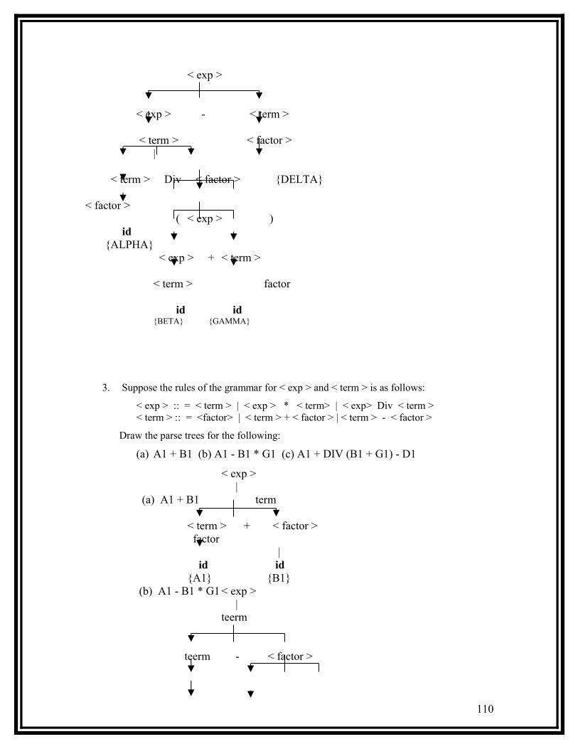
< exp >
< exp > - < term >
< term > < factor >|
< term > Div < factor > {DELTA}
< factor > ( < exp > )
id {ALPHA}
< exp > + < term >
< term > factor
id id{BETA} {GAMMA}
3. Suppose the rules of the grammar for < exp > and < term > is as follows:
< exp > :: = < term > | < exp > * < term> | < exp> Div < term >< term > :: = <factor> | < term > + < factor > | < term > - < factor >
Draw the parse trees for the following:
(a) A1 + B1 (b) A1 - B1 * G1 (c) A1 + DIV (B1 + G1) - D1
< exp > |
(a) A1 + B1 term
< term > + < factor > factor
| id id{A1} {B1}
(b) A1 - B1 * G1 < exp > |teerm
teerm - < factor >
110
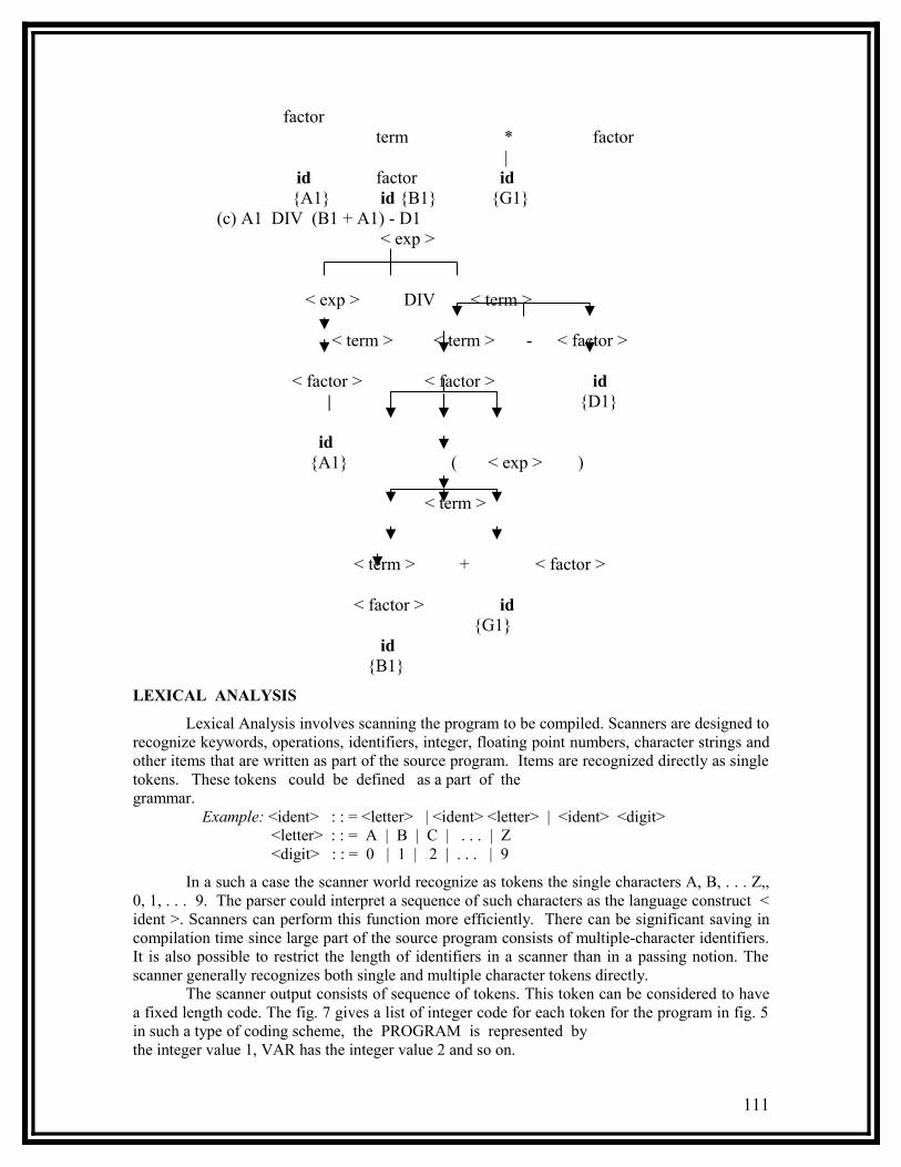
factor term * factor
| id factor id {A1} id {B1} {G1}
(c) A1 DIV (B1 + A1) - D1 < exp >
< exp > DIV < term >
< term > < term > - < factor >
< factor > < factor > id | {D1}
id {A1} ( < exp > )
< term >
< term > + < factor >
< factor > id {G1}
id {B1}
LEXICAL ANALYSIS
Lexical Analysis involves scanning the program to be compiled. Scanners are designed to recognize keywords, operations, identifiers, integer, floating point numbers, character strings and other items that are written as part of the source program. Items are recognized directly as single tokens. These tokens could be defined as a part of the grammar.
Example: <ident> : : = <letter> | <ident> <letter> | <ident> <digit> <letter> : : = A | B | C | . . . | Z <digit> : : = 0 | 1 | 2 | . . . | 9
In a such a case the scanner world recognize as tokens the single characters A, B, . . . Z,, 0, 1, . . . 9. The parser could interpret a sequence of such characters as the language construct < ident >. Scanners can perform this function more efficiently. There can be significant saving in compilation time since large part of the source program consists of multiple-character identifiers. It is also possible to restrict the length of identifiers in a scanner than in a passing notion. The scanner generally recognizes both single and multiple character tokens directly.
The scanner output consists of sequence of tokens. This token can be considered to have a fixed length code. The fig. 7 gives a list of integer code for each token for the program in fig. 5 in such a type of coding scheme, the PROGRAM is represented by the integer value 1, VAR has the integer value 2 and so on.
111

Token Program VAR BEGIN END END INTEGER FORCode 1 2 3 4 5 6 7
Token READ WRITE To Do ; : ,Token : = + - K DIV ( )
Token : = + - K DIV ( )Code 15 16 17 18 17 20 21
Token Id IntCode 22 23
Fig. 7 Token Coding Scheme
For a keyword or an operator the token loading scheme gives sufficient information. In the case of an identifier, it is also necessary to supply particular identifier name that was scanned. It is true for the integer, floating point values, character-string constant etc. A token specifier can be associated with the type of code for such tokens. This specifier gives the identifier name, integer value, etc., that was found by the scanner.
Some scanners enter the identifiers directly into a symbol table. The token specifier for the identifiers may be a pointer to the symbol table entry for that identifier.
The functions of a scanner are:
The entire program is not scanned at one time. Scanner is a operator as a procedure that is called by the processor when it needs
another token. Scanner is responsible for reading the lines of the source program and possible for
printing the source listing. The scanner, except for printing as the output listing, ignores comments. Scanner must look into the language characteristics.
Example: FOTRAN : Columns 1 - 5 Statement number : Column 6 Continuation of line
: Column 7 . 22 Program statement PASCAL : Blanks function as delimiters for tokens
: Statement can be continued freely : End of statement is indicated by ; (semi column)
Scanners should look into the rules for the formation of tokens.
Example: 'READ': Should not be considered as keyword as it is within quotes. i.e., all string within quotes should not be considered as token.
Blanks are significant within the quoted string. Blanks has important factor to play in different language
Example 1: FORTRAN Statement:
Do 10 I = 1, 100 ; Do is a key word, I is identifier, 10 is the statement number Statement: Do 10 I = 1 ;It is an identifier Do 10 I = 1
Note: Blanks are ignored in FORTRAN statement and hence it is a assignment statement. In this case the scanner must look ahead to see if there is a comma (,) before it can decide in the proper identification of the characters
112

Do.
Example 2: In FORTRAN keywords may also be used as an identifier. Words such as IF, THEN, and ELSE might represent either keywords or variable names.
IF (THEN .EQ ELSE) THENIF = THEN
ELSETHEN = IF
ENDIF
Modeling Scanners as Finite Automata
Finite automatic provides an easy way to visualize the operation of a scanner. Mathematically, a finite automation consists of a finite set of states and a set of transition from one state to another. Finite automatic is graphically represented. It is shown in fig, State is represented by circle. Arrow indicates the transition from one state to another. Each arrow is labeled with a character or set of characters that can be specified for transition to occur. The starting state has an arrow entering it that is not connected to anything else.
State Final State Transition Fig. 8
Example: Finite automata to recognize tokens is gives in fig. 9. The corresponding algorithm is given in fig. 10
0 - 9 A - Z
B A - Z
Fig. 9
Get first Input-characterIf Input-character in [ 'A' . . ' Z' ] then begin
while Input - character in [ 'A' . . 'Z', ' 0'. . ' 9' ] do begin
get next input - character End {while}
end {if first is [ 'A' .. ' Z' ] }else return (token-error)
Fig. 10
SYNTACTIC ANALYSIS
113
1
1
221
3

During syntactic analysis, the source programs are recognized as language constructs described by the grammar being used. Parse tree uses the above process for translation of statements, Parsing techniques are divided into two general classes:
-- Bottom up and -- Top down. Top down methods begin with the rule of the grammar that specifies the goal of the
analysis ( i.e., the root of the tree), and attempt to construct the tree so that the terminal nodes match the statement being analyzed.
Bottom up methods begin with the terminal nodes of the tree and attempt to combine these into successively high - level nodes until the root is reached.
OPERATOR PRECEDENCE PARSING
The bottom up parsing technique considered is called the operator precedence method. This method is loaded on examining pairs of consecutive operators in the source program and making decisions about which operation should be performed first.
Example: A + B * C - D (1)
The usual procedure of operation multiplication and division has higher precedence over addition and subtraction.
Now considering equation (1) the two operators (+ and *), we find that + has lower precedence than *. This is written as +⋖ * [+ has lower precedence *]
Similarly ( * and - ), we find that * ⋗ - [* has greater precedence -].The operation precedence method uses such observations to guide the parsing
process.
A + B * C - D (2) ⋖ ⋗
VA
R
BEG
INEN
DEN
D
INTE
GER
FO
R
REA
SW
RIT
E
TOD
O::
,: =+-
*D
IV)(
IdIn
t
PROGRAMVARBEGINEND
≐ ≐ ≐ ≐ ⋗ ⋗
⋖ ⋖ ⋖ ⋖ ⋖ ⋖ ⋗
<⋖⋖⋖
INTEGERFORREADWRITE
⋗ ⋗ ≐
≐ ≐
⋖
TODO ; :
⋖ ⋗ ⋗ ⋗ ⋗ ⋗ ⋗
⋖ ⋖ ⋖ ⋖ ⋖ ⋖ ⋖
⋗ ⋗ ⋗ ⋖ ⋗
⋖ ⋖
⋖
⋖ ⋖ ⋖ ⋖ ⋖ ⋖⋖⋖
114

,: = + -
⋗ ⋗ ⋗ ⋗ ⋗ ⋗ ⋗ ⋗
≐ ⋗ ⋗ ⋗ ⋗ ⋗ ⋗ ⋗ ⋗ ⋗ ⋗
⋖ ⋖ ⋗ ⋗ ⋗ ⋗ ⋗ ⋗
⋖ ⋖ ⋖⋖ ⋖ ⋖ ⋗⋖ ⋖ ⋖ ⋗⋗ ⋗ ⋗ ⋖
≐⋖ ⋖⋖ ⋖⋖ ⋖
*
DIV
)
(
⋗ ⋗ ⋗ ⋗ ⋗ ⋗
⋗ ⋗ ⋗⋗ ⋗ ⋗⋗ ⋗ ⋗⋗ ⋗ ⋗
⋗ ⋗ ⋗ ⋗⋖ ⋗ ⋗
⋗ ⋗ ⋖ ⋗⋗ ⋗ ⋖ ⋗⋖ ⋖ ⋖ ≐ ⋗ ⋗ ⋗
⋖ ⋖⋖ ⋖⋖ ⋖
id Int
⋗ ⋗ ⋗ ⋗ ⋗
⋗ ⋗ ⋗ ⋗⋗ ⋗ ⋗
⋗ ≐ ⋗ ⋗ ⋗ ⋗
⋗ ⋗ ⋗⋗ ⋗ ⋗
Fig 11 Precedence Matrix for the Grammar for fig 5
Equation (2) implies that the sub expression B * C is to be computed before either of the other operations in the expression is performed. In times of the parse tree this means that the * operation appears at a lower level than does either + or -. Thus a bottom up parses should recognize B * C by interpreting it in terms of the grammar, before considering the surrounding terms. The first step in constructing an operator-precedence parser is to determine the precedence relations between the operators of the grammar. Operator is taken to mean any terminal symbol (i.e., any token). We also haveprecedence relations involving tokens such as BEGIN, READ, id and ( . For the grammar in fig. 5, the precedence relations is given in the fig. 11.
Example: PROGRAM ≐ VAR ; These two tokens have equal precedence
Begin ⋖ FOR ; BEGIN has lower precedence over FOR. There are some values which do not follows precedence relations for comparisons.
Example: ; ⋗ END and END ⋗ ;
i.e., when ; is followed by END, the ' ; ' has higher precedence and when END is followed by ; the END has higher precedence.
In all the statements where precedence relation does not exist in the table, two tokens cannot appear together in any legal statement. If such combination occurs during parsing it should be recognized as error.
Let us consider some operator precedence for the grammar in fig. 5.
Example: Pascal Statement: BEGIN READ (VALUE);
These Pascal statements scanned from left to right, one token at a time. For each pair of operators, the precedence relation between them is determined. Fig. 12(a) shows the parser that has identified the portion of the statement delimited by the precedence relations ⋖ and ⋗ to be interpreted in terms of the grammar.
(a) . . . BEGIN READ ( id ) ⋖ ≐⋖ ⋗
(b) . . . BEGIN READ ( < N1 > ) ; ⋖ ≐ ≐ ⋗(c) . . . BEGIN < N2 > ;
(d) ... < N2 >
115

READ ( <N1 > )
id (VALUE)
Fig. 12
According to the grammar id may be considered as < factor > . (rule 12), <program > (rule 9) or a < id-list > (rule 6). In operator precedence phase, it is not necessary to indicate which non-terminal symbol is being recognized. It is interpreted as non-terminal < N1 >. Hence the new version is shown in fig. 12(b).
An operator-precedence parser generally uses a stack to save token that have been scanned but not yet parsed, so it can reexamine them in this way. Precedence relations hold only between terminal symbols, so < N1 > is not involved in this process and a relationship is determined between (and).
READ (<N1>) corresponds to rule 13 of the grammar. This rule is the only one that could be applied in recognizing this portion of the program. The sequence is simply interpreted as a sequence of some interpretation < N2 >. Fig. 12(c) shows this interpretation. The parser tree is given in fig. 12(d).
Note: (1) The parse tree in fig. 1 and fig. 12 (d) are same except for the name of the non-terminal symbols involved.
(2) The name of the non-terminals is arbitrarily chosen.
Example: VARIANCE ; = SUMSQ DIV 100 - MEAN * MEAN
(i) . . id 1 : = id 2 Div . . . <N1> ⋖ ≐ ⋖ ⋗
<id 2>(ii) . . . id 1 : = <N1> Div int -
⋖ ≐ ⋖ ⋖ ⋗ {SUMSQ}
(iii) . . . id 1 : = <N1> Div <N2> - <N1> <N2> ⋖ ≐ ⋖ ⋗
<id 2> int {SUMSQ} {100}
(iv) . . . . id 1 : = <N3> - id 3 * <N3> ⋖ ≐ ⋖ ⋖ ⋗
<N1> DIV <N2> id2 int{SUMSQ} {100}
v) . . . . id 1 : = <N3> - <N4> * id 4 ; <N4>⋖ ≐ ⋖ ⋖ ⋖ ⋗
id 3 {MEAN}
(vi) . . . id 1 : = <N3> - <N4> * <N5> <N5>
116

⋖ ≐ ⋖ ⋖ ⋗ id 4
{MEAN} (vii) . . . id 1 : = <N3> - <N6> <N6>
⋖ ≐ ⋖ ⋗ <N4> * <N5>
id 3 id 4 {MEAN} {MEAN}
(viii) . . . id : = <N7> <N7>⋖ ≐ ⋗
<N3> - <N6>
(ix) . . . <N8> <N8>
<N7>
<N3> <N6>
id 1 : = <N1> <N2> <N4> <N5> {VARIANCE} DIV *
id 2 int - id 3 id 4 {SUMSQ} {100} {MEAN} {MEAN}
SHIFT REDUCE PARSING The operation procedure parsing was developed to shift reduce parsing. This method
makes use of a stack to store tokens that have not yet been recognized in terms of the grammar. The actions of the parser are controlled by entries in a table, which is somewhat similar to the precedence matrix. The two main actions of shift reducingparsing are
Shift: Push the current token into the stack.
Reduce: Recognize symbols on top of the stack according to a rule of a grammar
Example: BEGIN READ ( id ) . . .
Steps Token Stream Stack 1. . . . BEGIN READ ( id ) . . .
117
Shift
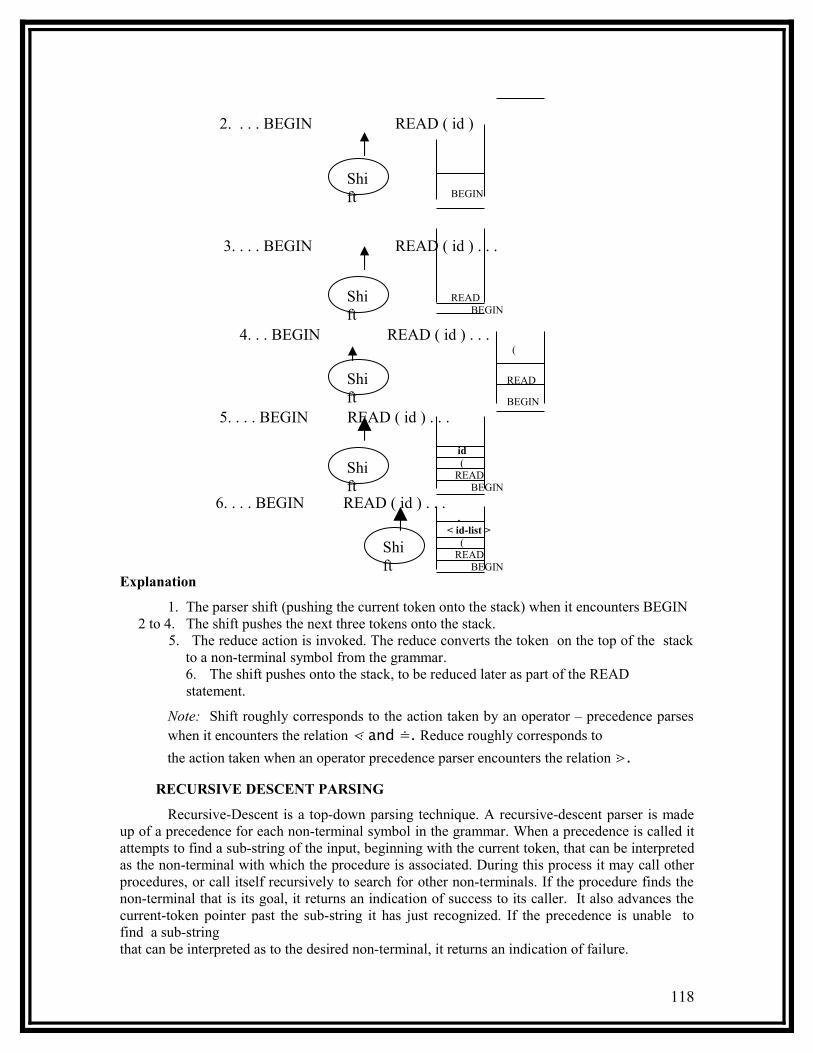
2. . . . BEGIN READ ( id )
BEGIN
3. . . . BEGIN READ ( id ) . . .
READ
BEGIN
4. . . BEGIN READ ( id ) . . . (
READ BEGIN
5. . . . BEGIN READ ( id ) . . .
id (
READ BEGIN
6. . . . BEGIN READ ( id ) . . . .
< id-list > (
READ BEGIN
Explanation
1. The parser shift (pushing the current token onto the stack) when it encounters BEGIN 2 to 4. The shift pushes the next three tokens onto the stack.
5. The reduce action is invoked. The reduce converts the token on the top of the stack to a non-terminal symbol from the grammar.6. The shift pushes onto the stack, to be reduced later as part of the READ
statement.
Note: Shift roughly corresponds to the action taken by an operator – precedence parses when it encounters the relation ⋖ and ≐. Reduce roughly corresponds to
the action taken when an operator precedence parser encounters the relation ⋗.
RECURSIVE DESCENT PARSING
Recursive-Descent is a top-down parsing technique. A recursive-descent parser is made up of a precedence for each non-terminal symbol in the grammar. When a precedence is called it attempts to find a sub-string of the input, beginning with the current token, that can be interpreted as the non-terminal with which the procedure is associated. During this process it may call other procedures, or call itself recursively to search for other non-terminals. If the procedure finds the non-terminal that is its goal, it returns an indication of success to its caller. It also advances the current-token pointer past the sub-string it has just recognized. If the precedence is unable to find a sub-stringthat can be interpreted as to the desired non-terminal, it returns an indication of failure.
118
Shift
Shift
Shift
Shift
Shift

Example: < read > : : = READ ( < id - list > )
The procedure for < read > in a recursive descent parser first examiner the next two input, looking for READ and (. If these are found, the procedures for < read > then call the procedure for < id - list >. If that procedure succeeds, the < read > procedure examines the next input token, looking for). If all these tests are successful, the < read > procedure returns an indication of success. Otherwise the procedure returns a failure.There are problems to write a complete set of procedures for the grammar of fig. 15. Example: The procedure for < id - list >, corresponding to rule 6 would be unable to decide between its alternatives since id and < id-list > can begin with id. <id-list > : : = id | < id-list >, id
If the procedure somehow decided to try the second alternative <id-list>, it would immediately call itself recursively to find an <id-list>. This causes unending chain. Top-down parsers cannot be directly used with a grammar that contains this kind of immediate left recursion.
Similarly the problem occurs for rules 3, 7, 10 and 11. Hence the fig. 13 shows the rules 3, 6, 7, 10 and 11 modification.
3 < dec - list > : : = < dec > { ; <dec > }6 < id - list > : : = id {; id }7 < stmt - list > : : = < stmt > { ; < stmt > }10 < exp > : : = < term > { + < term . | -- < term > }11 < term > : : = < factor > { + < factor > | Div < factor >.}
Fig. 13
Fig. 14 illustrates a recursive-descent parse of the READ statement: READ (VALUE); The modified grammar is considered in the procedure for the non-terminal <read > and < id-list >. It is assumed that TOKEN contains the type of the next input token.
PROCEDURE READ BEGIN
ROUND : = FALSEIf TOKEN + 8 { read } THEN BEGIN
advance to next tokenIF TOKEN + 20 { ( } THEN BEGIN
advance to next tokenIF IDLIST returns success THEN IF token = 21 { ) } THEN BEGIN
FOUND : = TRUE advance to next tokenEND { if ) }
END { if READ } IF FOUND = TRUE THEN return successelse failure
end (READ)Fig. 14
119

Procedure IDLISTbegin
FOUND = FALSEif TOKEN = 22 {id} then begin
FOUND : = TRUE advance to Next tokenwhile (TOKEN = 14 {,}) and (FOUND = TRUE) do begin
advance to next token if TOKEN = 22 {id} then
advance to next tokenelse
FOUND = FALSE End {while}End {if id}
if FOUND : = TRUE thenreturn success
elsereturn failure
end {IDLIST}
Fig. 15The fig. 15 IDLIST procedure shows an error message if ( , ) is not followed by a id. It
indicates the failure in the return statement. If the sequence of tokens such as " id, id " could be a legal construct according to the grammar, this recursive-descent technique would not work properly.
Fig. 16 shows a graphic representation of the recursive parsing process for thestatement being analyzed.
(i) In this part, the READ procedure has been invoked and has examined the tokens READ and ' ( " from the input stream (indicated by the dashed lines).
(ii) In this part, the READ has called IDLIST (indicated by the solid line), which has examined the token id.
(iii) In this part, the IDLIST has returned to READ indicating success; READ has then examined the input token.
Note that the sequence of procedure calls and token examinations has completely defined the structures of the READ statement. The parser tree was constructed beginning at the root, hence the term top-down parsing.
(i) (II) (iii)
READ READ READ ( ( ( id id
{ Value } { ValueFig. 16
Fig. 17 illustrates a recursive discard parse of the assignment statement.
Variance: = SUNSQ DIVISION - MEAN * MEAN
The fig. 17 shows the procedures for the non-terminal symbols that are
120
READ
READ
READ
IDLIST
IDLIST

involved in parsing this statement.
Procedure ASSIGNbegin
FOUND = FALSEif TOKEN = 22 {id} then begin
advance to Next token if TOKEN = 15 {: =} then begin advance to next token if EXP returns success then FOUND : = TRUE end {if : =}
if FOUND : = TRUE then return success
elsereturn failure
end {ASSIGN}Procedure EXP
begin FOUND = FALSE
If TERM returns success then begin
FOUND: = TRUEwhile ((TOKEN = 16 {+ } ) or (TOKEN = 17 { - } ) )
and (FOUND = TRUE) dobegin advance to next token if TERM returns success then
FOUND = FALSE end {while}
end {if TERM} if FOUND : = TRUE then
return success else
return failureend {EXP}
Procedure TERMbegin FOUND : = FALSE
If FACTOR returns success then begin
FOUND : = TRUEwhile ((TOKEN = 18 { * }) or (TOKEN = 19 {DIV })
and (FOUND = TRUE) dobegin advance to next token if TERM returns failure then
FOUND : = FALSE end {while}
121

end {if FACTOR} if FOUND : = TRUE then
return success else
return failure end {TERM}
Procedure FACTORbegin FOUND : = FALSE
if (TOKEN = 22 { id } ) or (TOKEN = 23 {int } ) then begin
FOUND : = TRUEadvance to next token
end { if id or int }else if TOKEN = 20 { ( } then begin
advance to next tokenif EXP returns success then if TOKEN = 21 { ) } then
begin(FOUND = TRUE) advance to next token
end { if ) }end {if ( }
if FOUND : = TRUE thenreturn success
elsereturn failure
end {FACTOR}
Fig. 17 Recursive-Descent Parse of an Assignment Statement
A step-by-step representation of the procedure calls and token examination is shown in fig. 1
(i) (ii) (iii)
id 1 : = id 1 : = id 1 : = { VARIANCE } { VARIANCE } {VARIANCE}
(iv) (v) (vi)
id 1 : = id 1 : = id 1 : =
122
ASSIGN ASSIGN
EXP
ASSIGN ASSIGN
EXP EXPEXP
ASSIGN
TERM
EXP

{VARIANCE} {VARIANCE} {VARIANCE}
-
DIV DIV
id 2 id 2 int id 2 int {SUMSQ} {SUMSQ} {100} {SUMSQ} {100}
(vii)
id 1 : = {VARIANCE}
-
DIV
id 2 int id 3 {SUMSQ} {100} {MEANS}
(viii)
id 1 : = (VARIANCE}
-
*
DIV DIV id 2 int id 3 id 4 {SUMSQ} {100} {MEANS} {MEANS}
Fig. 18 Step by step Representation for Variance : = SUMSQ Div 100 - MEAN * Mean
GENERATION OF OBJECT CODE
After the analysis of system, the object code is to be generated. The code generation technique used in a set of routine, one for each rule or alternative rule in the grammar. The routines that are related to the meaning of he compounding construct in the language is called the semantic routines.
When the parser recognizes a portion of the source program according to some rule of the grammar, the corresponding semantic routines are executed. These semantic routines generate object code directly and hence they are referred as code generation routines. The code generation routines that is discussed are designed for the use with the grammar in fig. .5. This grammar is used for code generations to emphasize the point that code generation techniques need not be associated with any particular parsing method.
123
TERM
ASSIGN
TERMTERMTERM
FACTOR FACTOR FACTOR FACTOR FACTOR
ASSIGN
FACTOR FACTOR
TERM
FACTOR
TERM
EXP
FACTOR FACTOR FACTOR FACTOR
TERM TERM
EXP

The parsing technique discussed in 1.3 does not follow the constructs specified by this grammar. The operator precedence method ignores certain non-terminal and the recursive-descent method must use slightly modified grammar.
The code generation is for the SIC/XE machine. The technique use two data structure:(1) A List (2) A Stack
List Count: A variable List count is used to keep a count of the number of items currently in the list. The token specifiers are denoted by ST (token)
Example: id ST (id) ; name of the identifierint ST (int) ; value of the integer, # 100
The code generation routines create segments of object code for the compiled program. A symbolic representation is given to these codes using SIC assemblerlanguage.
LC (Location Counter): It is a counter which is updated to reflect the next variable address in the compiled program (exactly as it is in an assembler).
Application Process to READ Statement:
(read)+ JSUB XREAD
WORD 1 < id - list > WORD VALUE
READ ( ) {VALUE}
Fig. 19(a) Parse Tree for Read
Using the rule of the grammar the parser recognizes at each step the left most sub-string of the input that can be interpreted. In an operator precedence parse, the recognition occurs when a sub-string of the input is reduced to some non-terminal <N i>.
In a recursive-descent parse, the recognition occurs when a procedure returns to its caller, indicating success. Thus the parser first recognizes the id VALUE as an < id - list >, and then recognizes the complete statement as a < read >.
The symbolic representation of the object code to be generated for the READ statement is as shown in fig. 19(b). This code consists of a call to a statement XREAD, which world be a part of a standard library associated with the compiler. The subroutine any program that wants to perform a READ operation can call XREAD. XREAD is linked together with the generated object program by a linking loader or a linkage editor. The technique is commonly used for the compilation of statements that perform voluntarily complex functions. The use of a subroutine avoids the repetitive generation of large amounts of in-line code, which makes the object program smaller.
The parameter list for XREAD is defined immediately after the JSUB that calls it. The first word is the number of variable that will be assigned values by the READ. The following word gives the addresses of three variables.
Fig. 19(c) shows the routines that might be used to accomplish the code generation.
1. < id - list > : : = idadd ST (id) to listadd 1 to List_count
2. < id - list > : : = < id - list >, idadd ST (id) to list
124

add 1 to LC List_Current3. < read > : : = READ (< id - list >)
generate [ + JSUB XREAD ] record external reference to XREAD
generate [WORD List - count]for each item on list of do begin
remove ST (ITEM) from listgenerate [WORD ST (ITEM)]
end List _count : = 0
Fig. 19 (c) Routine for READ Code Generation
The first two statements (1) and (2) correspond to alternative structure for < id - list >, that is < id - list > : : = id | < id - list >, id.
In each case the token specifies ST (id) for a new identifier being called to the < id - list > is inserted into the list used by the code-generation routine, and list-count is updated to reflect the insertion. After the entire < id-list > has been parsed, the list contains the token specifiers for all the identifiers that are part of the < id- list >. When the < read > statement is recognized, the token specifiers are removed from the list and used to generate the object code for the READ. Code-generation Process for the Assignment Statement
Example: VARIANCE: = SUMSQ DIV 100 - MEAN * MEAN
The parser tree for this statement is shown in fig. 20. Most of the work of parsing involves the analysis of the < exp > on the right had side of the " : = " statement.:
< assign >
< exp >
< exp > < exp > (term)
< term >
< term > < term > < factor >
< factor >< factor > < factor >
id : = id DIV int _ id * id {VARIANCE} { SUMSQ } {100} {MEAN} {MEAN}
Fig. 20
The parser first recognizes the id SUMSQ as a < factor > and < term > ; then it recognizes the int 100 as a < factor >; then it recognizes SUNSQ DIV 100 as a < term >, and so
125

forth. The order in which the parts of the statements are recognized is the same as the order in which the calculations are to be performed. A code-generation routine is called for each portion of the statement is recognized.
Example; For a rule < term >1: : = < term > 2 * < factor > a code is to be
generated.
The subscripts are used to distinguish between the two occurrences of < term > .The code-generation routines perform all arithmetic operations using register A. Hence
the multiple < term >2 * < factor > after multiplication is available in register A. Before multiplication one of the operand < term >2 must be located in A-register. The results after multiplication will be left in register A. So we need to keep track of the result left in register A by each segment of code that is generated. This is accomplished by extending the token-specifier idea to non-terminal nodes of the parse tree.
The node specifier ST (< term1>) would be set to rA, indicating that the result of the completion is in register A. the variable REGA is used to indicate the highest level node of the parse tree when value is left in register A by the code generated so far. Clearly there can be only one such node at any point in the code-generation process. If the value corresponding to a node is not in register A, the specifier for the node is similar to a token specifier: either a pointer to a symbol table entry for the variable that contains the value or an integer constant.
Fig. 21 shows the code-generation routine considering the A-register of the machine.
1. < assign > : : = id := < exp >GETA (< exp >) generate [ STA ST (id)]REGA : = null
2. <exp> :: =< term >ST < exp > : = ST (< term >)if ST < exp > = rA then REGA : = < exp >
3. < exp >1 : : = < exp >2 + < term >if SR (< exp >2) = rA then generate [ADD ST (< term >)]else if ST (< term >) = rA then generate [ADD ST (< exp >2)]else begin GETA (< EXP >2) generate [ADD ST(< term >)]endST (< exp >1) : = rAREGA : = < exp >1
4. < exp >1 : : = < exp >2 - < term >if ST (< exp >2) = rA then generate [SUB ST (< term >)]else begin GETA (< EXP >2) generate [ SUB ST (< term >)] end
126

SR (< exp >1) : = rAREGA : = < exp >1
5. < term > : : = < factor >ST (< term >) : = ST (< factor >)if ST (<term >) = rA then REGA : = < term >
6. < term >1 : : = < term >2 * < factor >if ST (< term >2) = rA then
generate [ MUL ST (< factor >)]else if S (< factor >) = rA then generate [ MUL ST (< term >2)]else begin GETA (< term >2) generate [ MUL SrT(< factor >)]endST (< term >1) : = rAREGA : = < term >1
7. < term > : : = < term >2 DIV < factor >if SR (< term >2) = rA then
generate [DIV ST(< factor >)]else begin GETA (< term >2) generate [ DIV ST (< factor >)]endSR (< term >1) : = rAREGA : = < term >1
< factor > : : = idST (< factor >) : = ST (id)
9. < factor > : : = intST (< factor >) : = ST (int)
10. < factor > : : = < exp >ST (< factor >) : = ST (< exp >) if ST (< factor >) = rA then REGA : = < factor >
Fig. 21 Code Generation Routines
If the node specifies for either operand is rA, the corresponding value is already in register A, the routine simply generates a MUL instruction. The node specifier for the other operand gives the operand address for this MUL. Otherwise, the procedure GETA is called. The GETA procedure is shown in fig. 22.
Procedure - GETA (NODE) begin
if REGA = null then generate [LDA ST (NODE) ]else if ST (NODE) π rA then begin
creates a new looking variable Tempi
127

generate [STA Tempi]record forward reference to Tempi
ST (REGA) : = Tempi
Generate [LDA ST (NODE)]end (if ≠ rA)ST(NODE) : = rAREGA : = NODE
end {GETA } Fig. 22
The procedure GETA generates a LDA instruction to load the values associated to <term> 2 into register A. Before loading the value into A-register, it confirms whether A is null. If it is not null it generates STA instruction to save the contents of register-A into Temp-variable. There can be number of Temp variable like Temp1, Temp2 . . . etc. The temporary variables used during a completion will be assigned storage location at the end of the object program. The node specifies for the node associated with the value previously in register A, indicated by REGA is reset to indicate the temporary variable used.
After the necessary instructions are generated, the code-generation routine sets ST (< term >1) and REGA to indicate that the value corresponding to < terms >1 is now in register A. This completes the code-generation action for the * operation.
The code-generation routine for ' + ' operation is the same as the ' * ' operation. The routine ' DIV ' and ' - ' are similar except that for these operations it is necessary for the first operand to be in register A. The code generation for < assign > consists of bringing the value to be assigned into register A (using GETA) and then generating a STA instruction.
The remaining rules in fig. 21 do not require the generation of any instruction since no computation and data movement is involved.
The object code generated for the assignment statement is shown in fig. 22.
LDA SUMSQDIV * 100STA TMP1
LDA MEANMUL MEANSTA TMP2
LDA TMP1
SUB TMP2
STA VARIABLE
Fig. 22
For the grammar < prog > the code-generation routine is shown in fig. 23. When <prog> is recognized, storage locations are assigned to any temporary (Temp) variables that have been used. Any references to these variables are then fixed in the object code using the same process performed for forward references by a one-pass assembler. The compiler also generates any modification records required to describe external references to library subroutine.
< prog > : : = PROGRAM < prog-name > VAR < dec list >BEGIN < stmp -- list > END.
generate [LDL RETADR]generate [RSUB]
for each Temp variable used do
128
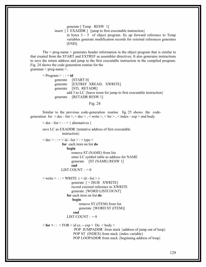
generate [ Temp RESW 1]insert [ J EXADDR ] {jump to first executable instruction}
in bytes 3 - 5 of object program. fix up forward reference to Temp variables generate modification records for external references generates [END].
The < prog-name > generates header information in the object program that is similar to that created from the START and EXTREF as assembler directives. It also generates instructions to save the return address and jump to the first executable instruction in the compiled program. Fig. 24 shows the code generation routine for the grammar < prog-name >.
< Program > : : = idgenerate [START 0]generate [EXTREF XREAD, XWRITE]generate [STL RETADR]
add 3 to LC {leave room for jump to first executable instruction}generate [RETADR RESW 1]
Fig. 24
Similar to the previous code-generation routine fig. 25 shows the code-generation for < dec - list >, < dec > , < write >, < for > , < index - exp > and body.
< dec - list > : : = { alternatives }
save LC as EXADDR {tentative address of first executable instruction}
< dec > : : = > id - list > : < type > for each item on list do
begin remove ST (NAME) from list enter LC symbol table as address for NAME generate [ST (NAME) RESW 1] end
LIST COUNT : = 0
< write > : : = WRITE ( < id - list > ) generate [ + JSUB XWRITE] record external reference to XWRITE generate [WORD LISTCOUNT]for each item on list do begin
remove ST (ITEM) from list generate [WORD ST (ITEM)]
endLIST COUNT : = 0
< for > : : = FOR < id ex -- exp > Do < body > POP JUMPADDR from stack {address of jump out of loop}
POP ST (INDEX) from stack {index variable} POP LOOPADDR from stack {beginning address of loop}
129

generate [LDA ST (INDEX)] generate [ADD #1] generate [ J LOOPADDR] insert [ JGT LC ] at location JUMPADDR
< index - exp > : : = id : = < exp > | TO < exp >2
GETA (< exp >;)Push LC onto stack {beginning addressing loop}Push ST (id) onto stack {index variable}Generate [STA ST (id)]Generate [ COMP ST (< exp > 2)]Push LC onto stack {address of jump out of loop}and 3 to LC [ leave room for jump instruction]REGA : = null
Fig. 25
There are no code-generation for the statements
< type > : : = INTEGER< stmt - list > : : = {either alternative}< stmt > : : = {any alternative}< body > : : = {either alternative}
For the Pascal program in fig. 1 the complete code-generation process is shown infig. 26.
1 STATS START 0 {Program Header} EXTREF XREAD, XREAD, XWRITE STL TETADR {Save return address} J {EXADDR} 2 RETADDR RESW 1 3 SUM RESW 1 SUMSQ RESW 1 I RESW 1 VALUE RESW 1 MEAN RESW 1 VARIANCE RESW 1 5 {EXADDR} LDA # 0 {SUM = 0} STA SUM 6 LDA # 0 {SUMSQ : = 0}
STA SUMSQ 7 LDA # 1 {FOR I : = 1 TO 100} {L1} STA I
COMP # 100JGT {L2}
9 + JSUB X READ {READ (VALUE) } WORD 1
WORD VALUE 10 LDA SUM {SUM : = SUM +
VALUE}
130

ADD VALUESTA SUM
11 LDA VALUE {SUMSQ : = SUMSQ * VALUE * VALUE}
MUL VALUEADD SUMSQSTA SUMSQLDA I {END OF FOR LOOP}ADD # 1J {L1}
13 {L2} LDA SUM {MEAN : = SUM DIVISION}
DIV # 100STA MEAN
14 LDA SUM {VARIABLE : = SUMSQ DIVDIV # 100 100 - MEAN * MEAN}STA TEMP1LDA MEANMUL MEANSTA TEMP2LDA TEMP1SUB TEMP2STA VARIANCE
15 +JSUB XWRITE {WRITE (MEAN, VARIANCE) }WORD 2WORD MEAN WORD VARIABLELDL RETADRRSUB
TEMP 1` RESW 1 {WORKING VARIABLE USED} TEMP 2 RESW 1
END
Fig. 25 Object Code Generated for Pascal Program
8.1 MACHINE DEPENDENT COMPILER FEATURES
At an elementary level, all the code generation is machine dependent. This is because, we must know the instruction set of a computer to generate code for it. There are many more complex issues involved. They are:
Allocation of register Rearrangement of machine instruction to improve efficiency of execution
Considering an intermediate form of the program being compiled normally does such types of code optimization. In this intermediate form, the syntax and semantics of the source statements have been completely analyzed, but the actual translation into machine code has not yet been performed. It is easier to analyze and manipulate this intermediate code than to perform the operations on either the source program or the machine code. The intermediate form made in a compiler, is not strictly dependent on the
131

machine for which the compiler is designed.
8.1.1 INTERMEDIATE FORM OF THE PROGRAM
The intermediate form that is discussed here represents the executable instruction of the program with a sequence of quadruples. Each quadruples of the form
Operation, OP1, OP2, result.Where
Operation - is some function to be performed by the object codeOP 1 & OP2 - are the operands for the operation and Result - designation when the resulting value is to be placed.
Example 1: SUM : = SUM + VALUE could be represented as + , SUM, Value, i, i1
: = i1 , , SUM
The entry i1, designates an intermediate result (SUM + VALUE); the second quadruple assigns the value of this intermediate result to SUM. Assignment is treated as a separate operation ( : =).
Example 2 : VARIANCE : = SUMSQ, DIV 100 -- MEAN * MEAN DIV, SUMSQ, #100, i1
*, MEAN, MEAN, i2
- , i1, i2, i3
: : = i3 , VARIABLE Note: Quadruples appears in the order in which the corresponding object code
instructions are to be executed. This greatly simplifies the task of analyzing the code for purposes of optimization. It is also easy to translate
into machine instructions.
For the source program in Pascal shown in fig. 1. The corresponding quadruples are shown in fig. 27. The READ and WRITE statements are represented with a CALL operation, followed by PARM quadruples that specify the parameters of the READ or WRITE. The JGT operation in quadruples 4 in fig. 27 compares the values of its two operands and jumps to quadruple 15 if the first operand is greater than the second. The J operation in quadruples 14 jumps unconditionally to quadruple 4.
Line Operation OP 1 OP 2 Result Pascal Statement
1. : = # 0 SUM SUM : = 0 2. : = # 0 SUMSQ SUMSQ : = 0 3. : = # 1 I FOR I : = 1 to 100 4. JGT I #100 (15) 5. CALL XREAD READ (VALUE) 6. PARAM VALUE 7. + SUM VALUE i1 SUM : = SUM + VALUE ; = i1 SUM 9. * VALUE VALUE i2 SUMSQ : = SUMSQ + VALUE 10. + SUMSQ i2 i3 * VALUE 11. : = i3 SUMSQ 12. + I #1 i4 End of FOR loop 13. : = i4 I
132
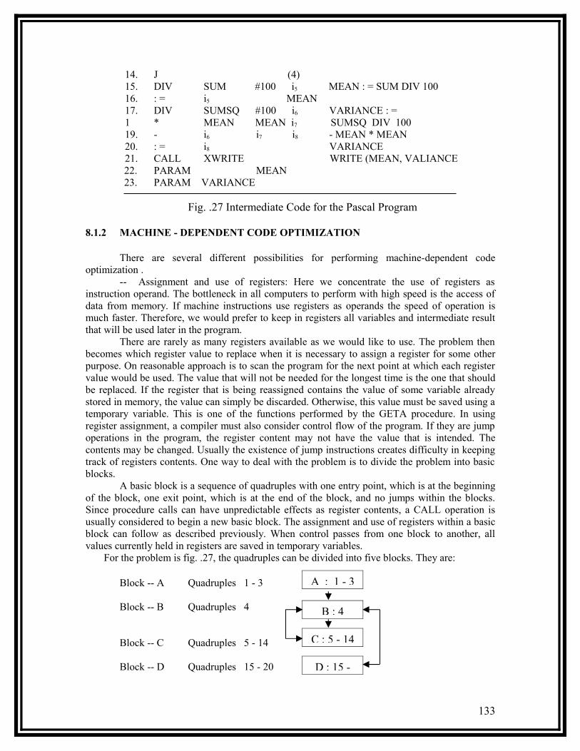
14. J (4) 15. DIV SUM #100 i5 MEAN : = SUM DIV 100 16. : = i5 MEAN 17. DIV SUMSQ #100 i6 VARIANCE : = 1 * MEAN MEAN i7 SUMSQ DIV 100 19. - i6 i7 i8 - MEAN * MEAN 20. : = i8 VARIANCE 21. CALL XWRITE WRITE (MEAN, VALIANCE22. PARAM MEAN23. PARAM VARIANCE
Fig. .27 Intermediate Code for the Pascal Program
8.1.2 MACHINE - DEPENDENT CODE OPTIMIZATION
There are several different possibilities for performing machine-dependent code optimization .
-- Assignment and use of registers: Here we concentrate the use of registers as instruction operand. The bottleneck in all computers to perform with high speed is the access of data from memory. If machine instructions use registers as operands the speed of operation is much faster. Therefore, we would prefer to keep in registers all variables and intermediate result that will be used later in the program.
There are rarely as many registers available as we would like to use. The problem then becomes which register value to replace when it is necessary to assign a register for some other purpose. On reasonable approach is to scan the program for the next point at which each register value would be used. The value that will not be needed for the longest time is the one that should be replaced. If the register that is being reassigned contains the value of some variable already stored in memory, the value can simply be discarded. Otherwise, this value must be saved using a temporary variable. This is one of the functions performed by the GETA procedure. In using register assignment, a compiler must also consider control flow of the program. If they are jump operations in the program, the register content may not have the value that is intended. The contents may be changed. Usually the existence of jump instructions creates difficulty in keeping track of registers contents. One way to deal with the problem is to divide the problem into basic blocks.
A basic block is a sequence of quadruples with one entry point, which is at the beginning of the block, one exit point, which is at the end of the block, and no jumps within the blocks. Since procedure calls can have unpredictable effects as register contents, a CALL operation is usually considered to begin a new basic block. The assignment and use of registers within a basic block can follow as described previously. When control passes from one block to another, all values currently held in registers are saved in temporary variables. For the problem is fig. .27, the quadruples can be divided into five blocks. They are:
Block -- A Quadruples 1 - 3
Block -- B Quadruples 4
Block -- C Quadruples 5 - 14
Block -- D Quadruples 15 - 20
133
A : 1 - 3
B : 4
C : 5 - 14
D : 15 -
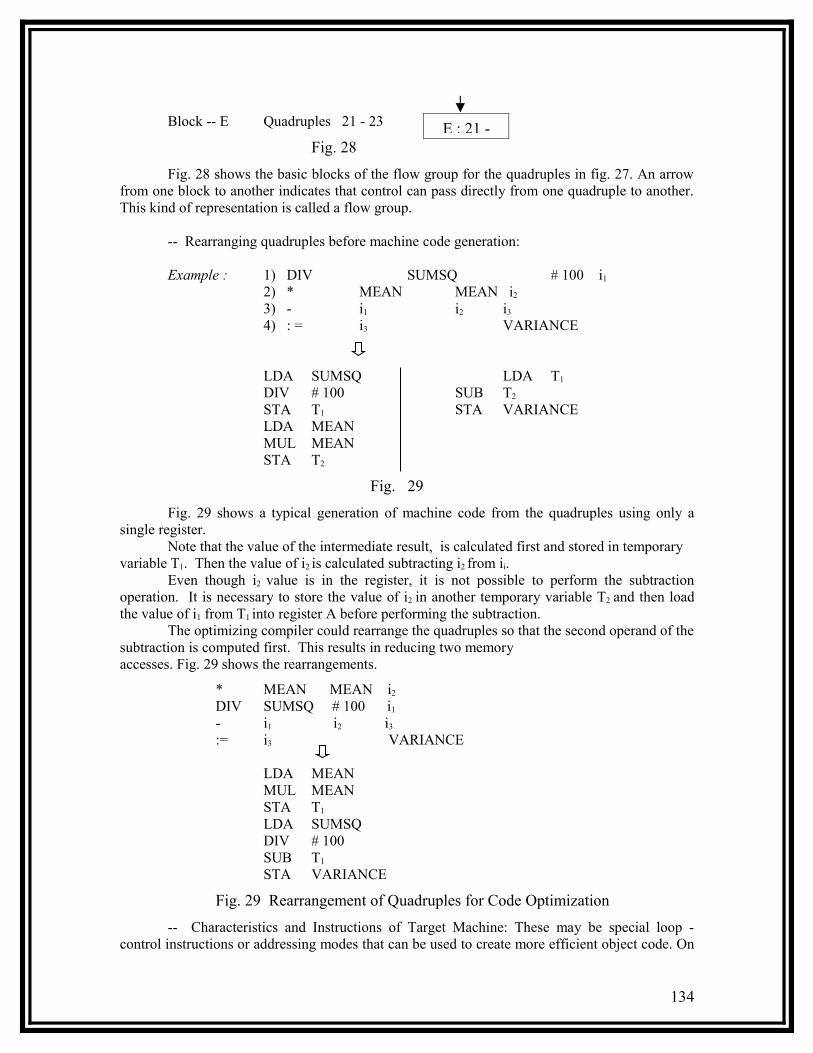
Block -- E Quadruples 21 - 23
Fig. 28
Fig. 28 shows the basic blocks of the flow group for the quadruples in fig. 27. An arrow from one block to another indicates that control can pass directly from one quadruple to another. This kind of representation is called a flow group.
-- Rearranging quadruples before machine code generation:
Example : 1) DIV SUMSQ # 100 i1
2) * MEAN MEAN i2
3) - i1 i2 i3
4) : = i3 VARIANCE
LDA SUMSQ LDA T1
DIV # 100 SUB T2
STA T1 STA VARIANCELDA MEANMUL MEANSTA T2
Fig. 29
Fig. 29 shows a typical generation of machine code from the quadruples using only a single register.
Note that the value of the intermediate result, is calculated first and stored in temporary variable T1. Then the value of i2 is calculated subtracting i2 from ii.
Even though i2 value is in the register, it is not possible to perform the subtraction operation. It is necessary to store the value of i2 in another temporary variable T2 and then load the value of i1 from T1 into register A before performing the subtraction.
The optimizing compiler could rearrange the quadruples so that the second operand of the subtraction is computed first. This results in reducing two memoryaccesses. Fig. 29 shows the rearrangements.
* MEAN MEAN i2
DIV SUMSQ # 100 i1
- i1 i2 i3
:= i3 VARIANCE
LDA MEANMUL MEANSTA T1
LDA SUMSQDIV # 100SUB T1
STA VARIANCE
Fig. 29 Rearrangement of Quadruples for Code Optimization
-- Characteristics and Instructions of Target Machine: These may be special loop - control instructions or addressing modes that can be used to create more efficient object code. On
134
E : 21 -

some computers there are high-level machine instructions that can perform complicated functions such as calling procedure and manipulating data structures in a single operation.
Some computers have multiple functional blocks. The source code must be rearranged to use all the blocks or most of the blocks concurrently. This is possible if the result of one block does not depend on the result of the other. There are some systems where the data flow can be arranged between blocks without storing the intermediate data in any register. An optimizing compiler for such a machine could rearrange object code instructions to take advantage of these properties.
Machine Independent Compiler Features
Machine independent compilers describe the method for handling structured variables such as arrays. Problems involved in compiling a block-structured languageindicate some possible solution.
3.1 STRUCTURED VARIABLES
Structured variables discussed here are arrays, records, strings and sets. The primarily consideration is the allocation of storage for such variable and then thegeneration of code to reference then.
Arrays: In Pascal array declaration -
(i) Single dimension array: A: ARRAY [ 1 . . 10] OF INTEGER
If each integer variable occupies one word of memory, then we require 10 words of memory to store this array. In general an array declaration is ARRAY [ l .. u ] OF INTEGER
Memory word allocated = ( u - l + 1) words.
(ii) Two dimension array : B : ARRAY [ 0 .. 3, 1 . . 3 ] OF INTEGER
In this type of declaration total word memory required is 0 to 3 = 4 ; 1 - 3 = 3 ; 4 x 3 = 12 word memory locations. In general: ARRAY [ l1 .. u1, l2 . . u2.] OF INTEGER Requires ( u1 - l1 + 1) * ( u2 - l2 + 1) Memory words
The data is stored in memory in two different ways. They are row-major and column major. All array elements that have the same value of the first subscript are stored in contiguous locations. This is called row-major order. It is shown in fig. 30(a). Another way of looking at this is to scan the words of the array in sequence and observe the subscript values. In row-major order, the right most subscript varies most rapidly.
0,1 0,2 0,3 0,4 0,5 0,1 1,2 1,3 1,4 1,5 2,1 2,2 2,3 2,4 2,5 . . .
Row 0 Row 1 Row 2
Fig. 30 (a)
Fig. 30(b) shows the column major way of storing the data in memory. All elements that have the same value of the second subscript are stored together; this is called column major order. In other words, the column major order, the left most subscript varies most rapidly.
To refer to an element, we must calculate the address of the referenced element relative to the base address of the array. Compiler would generate code to place the relative address in an index register. Index addressing mode is made easier to access the desired array element.
(1) One Dimensional Array: On a SIC machine to access A [6], the address is calculated by starting address of data + size of each data * number of preceding data.
135
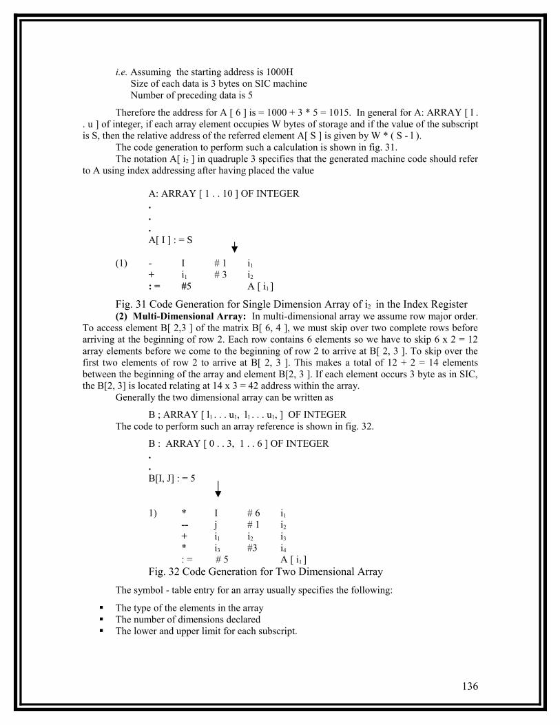
i.e. Assuming the starting address is 1000H Size of each data is 3 bytes on SIC machine Number of preceding data is 5
Therefore the address for A [ 6 ] is = 1000 + 3 * 5 = 1015. In general for A: ARRAY [ l . . u ] of integer, if each array element occupies W bytes of storage and if the value of the subscript is S, then the relative address of the referred element A[ S ] is given by W * ( S - l ).
The code generation to perform such a calculation is shown in fig. 31.The notation A[ i2 ] in quadruple 3 specifies that the generated machine code should refer
to A using index addressing after having placed the value
A: ARRAY [ 1 . . 10 ] OF INTEGER...A[ I ] : = S
(1) - I # 1 i1
+ i1 # 3 i2
: = #5 A [ i1 ]
Fig. 31 Code Generation for Single Dimension Array of i2 in the Index Register(2) Multi-Dimensional Array: In multi-dimensional array we assume row major order.
To access element B[ 2,3 ] of the matrix B[ 6, 4 ], we must skip over two complete rows before arriving at the beginning of row 2. Each row contains 6 elements so we have to skip 6 x 2 = 12 array elements before we come to the beginning of row 2 to arrive at B[ 2, 3 ]. To skip over the first two elements of row 2 to arrive at B[ 2, 3 ]. This makes a total of 12 + 2 = 14 elements between the beginning of the array and element B[2, 3 ]. If each element occurs 3 byte as in SIC, the B[2, 3] is located relating at 14 x 3 = 42 address within the array.
Generally the two dimensional array can be written as
B ; ARRAY [ l1 . . . u1, l1 . . . u1, ] OF INTEGERThe code to perform such an array reference is shown in fig. 32.
B : ARRAY [ 0 . . 3, 1 . . 6 ] OF INTEGER..B[I, J] : = 5
1) * I # 6 i1
-- j # 1 i2
+ i1 i2 i3
* i3 #3 i4
: = # 5 A [ i1 ]Fig. 32 Code Generation for Two Dimensional Array
The symbol - table entry for an array usually specifies the following:
The type of the elements in the array The number of dimensions declared The lower and upper limit for each subscript.
136

This information is sufficient for the compiler to generate the code required for array reference. Some of the languages line FORTRAN 90, the values of ROWS and COLUMNS are not known at completion time. The compiler cannot directly generate code. Then, the compiler create a descriptor called dope vector for the array. The descriptor includes space for storing the lower and upper bounds for each array subscript. When storage is allocated for the array, the values of these bounds are computed and stored in the descriptor. The generated code for one array reference uses the values from the descriptor to calculate relative addresses as required. The descriptor may also include the number of dimension for the array, the type of the array elements and a pointer to the beginning of the array. This information can be useful if the allocated array is passed as a parameter to another procedure.
In the compilation of other structured variables like recode, string and sets the same type of storage allocations are required. The compiler must store information concerning the structure of the variable and use the information to generate code to access components of the structure and it must construct a description for situation in which the required conformation is not known at compilation time.
8.3.1 MACHINE - INDEPENDENT CODE OPTIMIZATION
One important source of code optimization is the elimination of common sub-expressions. These are sub-expressions that appear at more than one port in the program and that compute the same value. Let us consider the example in fig. 33.
x, y : ARRAY [ 0 . . 10, 1 . . 10 ] OF INTEGER...FOR I : = 1 TO 10 DO X [ I, 2 * J - 1 ] : = [ I, 2 * J }
Fig. 33(a)
The sub-expression 2 * J is calculated twice. An optimizing compiler should generate code so that the multiplication is performed only once and the result is used in both places. Common sub-expressions are usually detected through the analysis of an intermediate form of the program. This intermediate form is shown in fig. 33(b).
Line Operation OP 1 OP 2 Result Pascal Statement
1. : = #1 I [Loop initialization] 2. JGT I #10 (20) 3. - I #1 i1 [Subscript calculation for x] 4. * i1 #10 i2
5. * #2 J i3 6. -- i3 #1 i4 7. -- i4 #1 i5
+ i2 i5 i6
9. * i6 #3 i7
10. -- I #1 i8 [Subscript Calculation for y] 11. * i8 #10 i9 12. * #2 J i10
13. -- i10 3 1 i11
137

14. + i9 i11 i12
15. * i12 # 3 i13
16. : = y [ i13 } x [ i17 ] [Assignment Operation] 17. + #1 I i17 [End of Loop]
1 : = i14 I
19. J (2)
20. [Next Statement]
Fig. 33(b)
Examining fig. 33(b), the sequence of quadruples, we observe that quadruples 5 and 12 are the same except for the name of the intermediate result produced. The operand J is not changed in value between quadruples 5 and 12. It is not possible to reach quadruple 12 without passing through quadruple 5 first because the quadruples are part of the same basic block. Therefore, quadruples 5 and 12 compute the same value. This means we can delete quadruple 12 and replace any reference to its result ( i10 ), with the reference to i3, the result of quadruple 5. this information eliminates the duplicate calculation of 2 * J which we identified previously as a common expression in the source statement.
After the substitution of i3 for i10 , quadruples 6 and 13 are the same except for the name of the result. Hence the quadruple 13 can be removed and substitute i4 for i11 wherever it is used. Similarly quadruple 10 and 11 can be removed because they are equivalent to quadruples 3 and 4.
Line Operation OP 1 OP 2 Result Pascal Statement
1. : = #1 I [Loop initialization] 2. JGT I #10 (16) 3. - I #1 i1 [Subscript calculation for x] 4. * i1 #10 i2
5. * # 2 J i3 6. - i3 #1 i4 7. - i4 # 1 i5
+ i2 i5 i6
9. * i6 # 3 i7
10. + i2 i4 i12 [Subscript Calculation for y]
11. * i12 # 3 i13 12. : = y [ i13 ] x [i7 ] [assignment Operation]
13. + #1 I i14 [End of Loop]
14. : = i14 I 15. J (2) 16. [Next Statement]
Fig. 34
Names i1 have been left unchanged, except for the substitutions first described, to make the compromise with fig. 33(b) easier. This optimized code has only 15 quadruples and hence the time taken is reduced.
Another method of code optimization is the removal of loop invariants. There are sub-expressions within the loop whose values do not change from one iteration of the loop to the next. Thus the values can be calculated once, before the loop is entered, rather than being recalculated for each iteration. In the example shows in fig. 33(a), the loop-invariant computation is the term 2
138

* J [quadruple 5 fig. 34]. The result of this computation depends only on the operand J, which does not change the value during the execution of the loop. Thus we can move quadruple 5 in fig. 34 to a point immediately before the loop is entered. A similar arrangement can be applied to quadruples 6 and 7. Fig. 35 shows the sequence of quadruples that result from these modification.
The total number of quadruples remains the same as fig. 34, however, the number of quadruples within the body of the loop has been reduced from 14 to 11. Our modification have reduced the total number of quadruples for one execution of the FOR from 181 [Fig. 23 (b) ], to 114 [Fig 25], which saves a substantial amount of time.
Line Operation OP 1 OP 2 Result Pascal Statement
1. * #2 J i3 {Commutation of invariants} 2. - i3 #1 i4 3. - i4 #1 i5 4. : = #1 I {Loop Initialization} 5. JGT I #10 (16) 6. - I #1 i1
7. * i1 #10 i2 {Subscript calculation for x} + i2 i5 i6
9. * i6 #3 i7
10. + i2 i4 i12 {Subscript Calculation for y} 11. * i12 #3 i13 12. : = y [ i13 ] x [i7 ] {assignment Operation} 13. + #1 I i14 {End of Loop} 14. : = i14 I 15. J (5) 16. {Next Statement}
Fig. 35
-- The optimization can be obtained by rewriting the source program.
Example; The statement in fig. 36(a) could be written as shown in fig. 36 (b).
FOR I : = 1 To 10 Do x [ I, 2 * J - 1 ] : = y [ I, 2 * J ]
Fig. 36(a)
T1 : = 2 * J ;T2 : = T1 -- 1 ;FOR : = 1 To 10 Do
x [ I, T2 ] : = y[ I, T1]
Fig. 36(b)
This would achieve only a part of the benefits realized by the optimization process described. Some time the statement in fig. 36(a) is preferable because it is clearer than the modified version involving T1 and T2. An optimizing compiler should allow the programmer to write source code that is clearer and easy to read and it shouldcompile such a program into machine code that is efficient to execute.
-- Code optimization of another source is the substitution of a more efficient operation for a less efficient one.
139
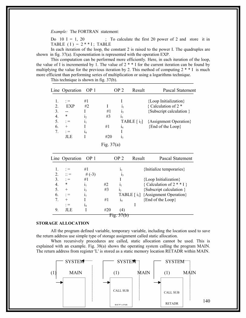
Example: The FORTRAN statement:
Do 10 I = 1, 20 ; To calculate the first 20 power of 2 and store it in TABLE ( I ) = 2 * * I ; TABLEIn each iteration of the loop, the constant 2 is raised to the power I. The quadruples are
shown in fig. 37(a). Exponentiation is represented with the operation EXP.This computation can be performed more efficiently. Here, in each iteration of the loop,
the value of I is incremented by 1. The value of 2 * * I for the current iteration can be found by multiplying the value for the previous iteration by 2. This method of computing 2 * * I is much more efficient than performing series of multiplication or using a logarithms technique.
This technique is shown in fig. 37(b).
Line Operation OP 1 OP 2 Result Pascal Statement
1. : = #1 I {Loop Initialization} 2. EXP #2 I i1 { Calculation of 2 * 3. -- I #1 i5 {Subscript calculation } 4. * i2 #3 i3 5. : = i1 TABLE [ i2] {Assignment Operation} 6. + I #1 i4 {End of the Loop}
7. : = i4 I JLE I #20 i3
Fig. 37(a)
Line Operation OP 1 OP 2 Result Pascal Statement
1. : = #1 i1 {Initialize temporaries} 2. :: = # (-3) i3 3. : = #1 I {Loop Initialization} 4. * i1 #2 i1 { Calculation of 2 * * I } 5. + i3 #3 i3 {Subscript calculation } 6. : = i1 TABLE [ i3] {Assignment Operation} 7. + I #1 i4 {End of the Loop} : = i4 I 9. JLE I #20 (4)
Fig. 37(b)
STORAGE ALLOCATION
All the program defined variable, temporary variable, including the location used to save the return address use simple type of storage assignment called static allocation.
When recursively procedures are called, static allocation cannot be used. This is explained with an example. Fig. 38(a) shows the operating system calling the program MAIN. The return address from register 'L' is stored as a static memory location RETADR within MAIN.
SYSTEM SYSTEM SYSTEM
(1) MAIN (1) MAIN (1) MAIN
140
CALL SUB
RETADR
CALL SUB
RETADR
RETADR
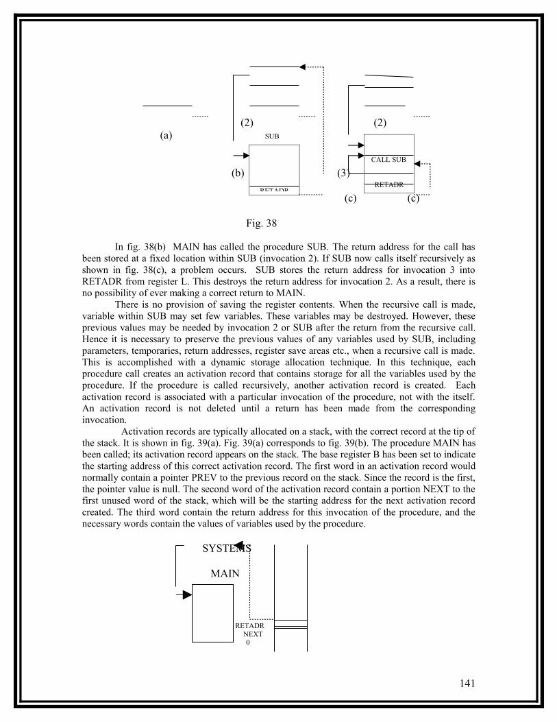
(2) (2)(a) SUB
(b) (3)
(c) (c)
Fig. 38
In fig. 38(b) MAIN has called the procedure SUB. The return address for the call has been stored at a fixed location within SUB (invocation 2). If SUB now calls itself recursively as shown in fig. 38(c), a problem occurs. SUB stores the return address for invocation 3 into RETADR from register L. This destroys the return address for invocation 2. As a result, there is no possibility of ever making a correct return to MAIN.
There is no provision of saving the register contents. When the recursive call is made, variable within SUB may set few variables. These variables may be destroyed. However, these previous values may be needed by invocation 2 or SUB after the return from the recursive call. Hence it is necessary to preserve the previous values of any variables used by SUB, including parameters, temporaries, return addresses, register save areas etc., when a recursive call is made. This is accomplished with a dynamic storage allocation technique. In this technique, each procedure call creates an activation record that contains storage for all the variables used by the procedure. If the procedure is called recursively, another activation record is created. Each activation record is associated with a particular invocation of the procedure, not with the itself. An activation record is not deleted until a return has been made from the corresponding invocation. Activation records are typically allocated on a stack, with the correct record at the tip of the stack. It is shown in fig. 39(a). Fig. 39(a) corresponds to fig. 39(b). The procedure MAIN has been called; its activation record appears on the stack. The base register B has been set to indicate the starting address of this correct activation record. The first word in an activation record would normally contain a pointer PREV to the previous record on the stack. Since the record is the first, the pointer value is null. The second word of the activation record contain a portion NEXT to the first unused word of the stack, which will be the starting address for the next activation record created. The third word contain the return address for this invocation of the procedure, and the necessary words contain the values of variables used by the procedure.
SYSTEMS
MAIN
RETADR NEXT
0
141
RETADR
CALL SUB
RETADR

Stack
Fig. 39 (a)
SYSTEM (1) MAIN
B
SUBStack
Fig. 39(b)
In fig. 39 (b), MAIN has called the procedure SUB. A new activation record has been created on the top of the stack, with register B set to indicate this new current record. The pointers PREV and NEXT in the time records have been set as shown.
SYSTEM
(1) MAIN
B
Fig. 39 (c) StackIn fig. 39(c), SUB has called itself recursively another activation record has been created
for this current invocation for SUB. Note that the return address and variable values for the two invocations of SUB are kept separate by this process.
When a procedure returns to its caller, the current activation record (which corresponds to the most recent invocation) is deleted. The pointer PREV in the deleted record is used to reestablish the previous activation record as the current one, and execution continues.
SYSTEM (1) MAIN
142
CALL SUB
VariablesFor SUB
RETADR NEXT PREV
VariableFor MAINRETADR
NE XT0
stacl
CALL SUB
VariablesFor SUB
RETADR NEXT
PREVVariable
For MAIN
RETADR
NEXT
PREVVariable
For MAINRETADR
NEXT0
CALL SUB
VariablesFor SUB
RETADR NEXT PREV
VariableFor MAINRETADR
NEXT0
CALL SUB

B
SUB
Fig. 39(d) Stack
Fig. 39(d) shows the stack as it would appear after SUB returns from the recursive call. Register B has been reset to point to the instruction record for the previous invocation of SUB. The return address and all the variable values in this activation record are exactly the same as they were before the recursive call.
This technique is called automatic allocation of storage. When the technique is used the compiler must generate code for the reference to variables using some sort of relative addressing. In our example the compiler assigns to each variable an address that is relative to the beginning of the activation record, instead of an actual location within the object program. The address of the current activation record is, by convention contained in register B, so a reference to a variable is translated as an instruction that uses base relative addressing. The displacement in this instruction is the relative address of the variable within the activation record.
The compiler must also generate additional code to manage the activation records themselves. At the beginning of each procedure there must be code to create a new activation record, linking it to the previous one and setting the appropriate pointers as shown in fig. 39. This code is often called a prologue for the procedure. At the end of the procedure, there must be code to delete the current activation record, resulting pointers as needed. This code is called an epilogue.
Example: IN FOTRAN 90 :ALLOCATE (MATRIX (ROWS, COLUMNS) ) allocation storage for the dynamic array MATRIX with the specified dimensions.
DE-ALLOCATE MATRIX releases the storage assigned to MATRIX by a previous ALLOCATE.
IN PASCAL: NEW (P)allocates storage for a variable and sets the pointer P to indicate the variable just created.DISPOSE (P)releases the storage that was previously assigned to the variable pointed to by P.
In C : MALLCO (SIZE) ; allocate a block of specified size ...
FREE (P) ; frees the storage indicated by pointer P.
A variable that is dynamically allocated in this way does not occupy a fixed location in an activation record, so it cannot be referenced directly using base relative addressing. Such a variable is usually accessed using indirect addressing through a pointer variable P. Since P does occupy a fixed location in the activation record, it can be addressed in the usual way.
The mechanism to allocate a storage memory to a variable can be done in any of the following ways:
A NEW or MALLOC statement would be translated into a request by the operating system for an area of storage of the required size.
143

The required allocation is handled through a run-time support procedure associated with the compiler. With this method, a large block of free storage called a heap is obtained from the operating system at the beginning of the program. Allocations of the storage from the heap are managed by the run-time procedure. In some systems, the program need not free memory for storage. A run-time garbage collection procedure scans the pointer in the program and reclaims areas from the heap that are no longer used.
8.3.3 BLOCK - STRUCTURED LANGUAGE
A block is a unit that can be divided in a language. It is a portion of a program that has the ability to declare its own identifiers. This definition of a block is also meet the units such as procedures and functions.
Let us consider a Pascal program with number of procedure blocks as shown in fig. 40.Each procedure corresponds to a block. Note that blocks are rested within other blocks.
Example: Procedures B and D are rested within procedure A and procedure C is rested within procedure B. Each block may contain a declaration of variables. A block may also refer to variables that are defined in any block that contains it, provided the same names are not redefined in the inner block. Variables cannot be used outside the block in which they are declared.
In compiling a program written in a blocks structured language, it is convenient to number the blocks as shown in fig. 40. As the beginning of each new block is recognized, it is assigned the next block number in sequence. The compiler can then construct a table that describes the block structure. It is illustrated in fig. 41. The block- level entry gives the nesting depth for each block. The outer most block number that is one greater than that of the surrounding block.
PROCEDURE A ; VAR X, Y, Z : INTEGER ;
:PROCEDURE B ;
VAR W, X, Y : REAL ; :PROCEDURE C ;
VAR W, V : INTEGER ; 1 : 3 2
END { C }; :
END { B }; :
PROCEDURE D ; VAR X, Z : CHAR ;
. 2 .
END { D};END { A};
Fig. 40 Nested Blocks in a Program
Block Surrounding
144

Name Number Level BlockABCD
1234
1232
--121
Fig. 41
Since a name can be declared more than once in a program (by different blocks), each symbol-table entry for an identifier must contain the number of the declaring block. A declaration of an identifier is legal if there has been no previous declaration of that identifier by the current block, so there can be several symbolic table entries for the same name. The entries that represent declaration of the same name by different blocks can be linked together in the symbol table with a chain of pointers.
When a reference to an identifier appears in the source program, the compiler must first check the symbol table for a definition of that identifier by the current block. If not such definition is found, the compiler looks for a definition by the block that surrounds the current one, then by the block that surrounds that and so on. If the outermost block is reached without finding a definition of the identifier, then the reference is an error.
The search process just described can easily be implemented within a symbol table that uses hashed addressing. The hashing function is used to locate one definition of the identifier. The chain of definitions for that identifier is then searched for the appropriate entry.
Most block-structured languages make use of automatic storage allocation. The variables that are defined by a block are stored in an activation record that is created each time the block is entered. If a statement refers to a variable that is declared within the current block, this variable is present in the current activation record, so it can be accessed in the usual way. It is possible to refer to a variable that is declared in some surrounding block. In that case, the most recent activation record for that block must be located to access the variable.
Stack(a) (b)
Fig. 42 Use of Display for Procedure
A data structure called display is used to access a variable in surrounding blocks. The display contains pointers to the most recent activation records for the current block and for all blocks that surround the current one in the source program. When a block refers to a variable that is declared in some surrounding block, the generated object code uses the display to find the activation record that contains this variable.
Example:
145
ActivationRecord for
C
ActivationRecord for
B
ActivationRecord for
C
ActivationRecord for
C
Activatio
C
B
AC
B
A

When a procedure calls itself recursively thus an activation record is created on the stack as a result of the call. Assume procedure C calls itself recursively. It is shown in fig. 42(b) the record for C is created on the stack as a result of the call. Any reference to a variable declared by C should use this most recent activation record ; the display pointer for C is changed accordingly. Variables that correspond to the previous invocation of C are not accessible for the movement, so there is no display pointer to this activation record.
Stack Display Fig 42(c)
Now if procedure 'C' call procedure D the resulting stack and display are as illustrated in fig. 42(c) . An activation record for D has been created in the usual way and added to the stack. Note, that the display now contains only two pointers: one each to the activation records for D and A. This is because procedure D cannot refer to variable in B or C, except through parameters that are passed to it, even though it is called from C.According to the rules for the scope of names in as block-structured language, procedure D can refer only to variable that are declared by D or by some block that contains D in the source program.
8.4 COMPILER DESIGN OPTIONS
The compiler design is briefly discussed in this section. The compiler is dividedinto single pass and multi pass compilers.
4.1. COMPILER PASSES
One pass compiler for a subset of the Pascal language was discussed in section 1. In this design the parsing process drove the compiler. The lexical scanner was called when the parser needed another input token and a code-generation routine was invoked as the parser recognized each language construct. The code optimization techniques discussed cannot be applied in total to one-pass compiler without intermediate code-generation. One pass compiler is efficient to generate the object code.
One pass compiler cannot be used for translation for all languages. FORTRAN and PASCAL language programs have declaration of variable at the beginning of the program. Any variable that is not declared is assigned characteristic by default.
One pass compiler may fix the formal reference jump instruction without problem as in one pass assembler. But it is difficult to fix if the declaration of an identifier appears after it has been used in the program as in some programming languages.
146
ActivationRecord for
C ActivationRecord for
B
ActivationRecord for AActivation D
A

Example: X : = Y * Z
If all the variables x, y and z are of type INTEGER, the object code for this statement might consist of a simple integer multiplication followed by storage of the result. If the variable are a mixture of REAL and INTEGER types, one or more conversion operations will need to be included in the object code, and floating point arithmetic instructions may be used. Obviously the compiler cannot decide what machine instructions to generate for this statement unless instruction about the operands is available. The statement may even be illegal for certain combinations of operand types. Thus a language that allows forward reference to data items cannot be compiled in one pass.
Some programming language requires more than two passes. Example : ALGOL-98 requires at least 3 passes.
There are a number of factors that should be considered in deciding between one pass and multi pass compiler designs.
(1) One Pass Compiles: Speed of compilation is considered important. Computer running students jobs tend to spend a large amount of time performing compilations. The resulting object code is usually executed only once or twice for each compilation, these test runs are not normally very short. In such an environment, improvement in the speed of compilation can lead to significant benefit in system performance and job turn around time.
(2) Multi-Pass Compiles: If programs are executed many times for each compilation or if they process large amount of data, then speed of executive becomes more important than speed of compilation. In a case, we might prefer a multi-pass compiler design that could incorporate sophisticated code-optimization technique.
Multi-pass compilers are also used when the amount of memory, or other systems resources, is severely limited. The requirements of each pass can be kept smaller if the work by compilation is divided into several passes.
Other factors may also influence the design of the compiler. If a compiler is divided into several passes, each pass becomes simpler and therefore, easier to understand, read and test. Different passes can be assigned to different programmers and can be written and tested in parallel, which shortens the overall time require for compiler construction.
INTERPRETERS
An interpreter processes a source program written in a high-level language. The main difference between compiler and interpreter is that interpreters execute a version of the source program directly, instead of translating it into machine code.
An interpreter performs lexical and syntactic analysis functions just like compiler and then translates the source program into an internal form. The internal form may also be a sequence of quadruples.
After translating the source program into an internal form, the interpreter executes the operations specified by the program. During this phase, an interpreter can be viewed as a set of subtractions. The internal form of the program drives the execution of this subtraction.
The major differences b/w interpreter and compiler are:
Interpreters Compilers
147

In some languages the type of a variable can change during the execution of a program. Dynamic scoping is used, in which the variable that are referred to by a function or a subroutines are determined by the sequence of calls made during execution, not by the nesting of blocks in the source program. It is difficult to compile such language efficiently and allow for dynamic changes in the types of variables and the scope of names. These features can be more easily handled by an interpreter that provides delayed binding of symbolic variable names to data types and locations.
4.3 P-CODE COMPILERS
P-Code compilers also called byte of code compilers are very similar in concept to interpreters. A P-code compiler, intermediate form is the machine language for a hypothetical computers, often called pscudo-machine or P-machine. The process of using such a P-code is shown in fig, 43.
The main advantage of this approach is portability of software. It is not necessary for the compiler to generate different code for different computers, because the P-code object program can be executed on any machine that has a P-code interpreter. Even the compiler itself can be transported if it is written in the language that it compiles. To accomplish this, the source version of the compiler is compiled into P-code; this P-code can then be interpreted on another compiler. In this way P-code compiler can be used without modification as a wide variety of system if a P-code interpreter is written for each different machine.
1) The process of translating a source program into some internal form is simpler and faster
The process of translating a source program into some internal form is slower than interpreter.
2) Execution of the translated program is much slower.
Executing machine code is much faster.
3) Debugging facilities can be easily provided.
Provision of bugging facilities are difficult and complicated.
4) During execution the interpreter produce symbolic dumps of data values, trace of program execution related to the source statement.
The compiler does not produce symbolic dumps of date value. Debugging tools are required for trace the program.
5) Program testing can be done effectively using interpreter as the operation on different data can be traced.
It is difficult to test as the compiler execution file gives the final result.
6) Easy to handle dynamic scoping
Difficult to handle dynamic scooping
148

Source Program
Object Program P - Code
Fig. 43
The design of a P-machine and the associated P-code is often related to the requirements of the language being compiled. For example, the P-code for a Pascal compiler might include single P-instructions that perform:
Array subscript calculation Handle the details of procedure entry and exit and Perform elementary operation on sets
This simplifies the code generation process, leading to a smaller and more efficient compiler.
The P-code object program is often much smaller than a corresponding machine code program. This is particularly useful on machines with severely limited memory size.
The interpretive execution of P-code program may be much slower than the execution of the equivalent machine code. Many P-code compilers are designed for a single user running on a dedicated micro-computer systems. In that case, the speed of execution may be relatively insignificant because the limiting factor is system performance may be the response time and " think time " of the user.
If execution speed is important, some P-code compilers support the use of machine-language subtraction. By rewriting a small number of commonly used routines in machine language, rather than P-code, it is often possible to improve the performance. Of course, this approach sacrifices some of the portability associated with the use of P-code compilers.
8.4.2 COMPILER-COMPILERS
Compiler-Compiler is software tool that can be used to help in the task of compiler construction. Such tools are also called Compiler Generators or Translator - writing system.
The process of using a typical compiler-compiler is shown in fig. 44. The compiler writer provides a description of the language to be translated. This description may consists of a set of lexical rules for defining tokens and a grammar for the source language. Some compiler-compilers use this information to generate a scanner and a parses directly. Others create tables for use by standard table-driven scanning and parsing routines that are supplies by the compiler - compiler.
Lexical Ruler
149
Compiler P-CodeCompiler
P - CodeInterprete
rExecute
Compiler-Compiler
Scanner
Parser
CodeGenerator
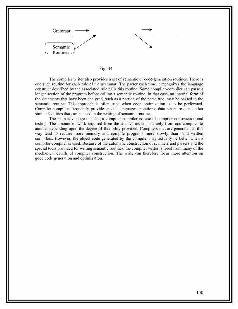
Grammar
Semantic Routines
Fig. 44
The compiler writer also provides a set of semantic or code-generation routines. There is one such routine for each rule of the grammar. The parser each time it recognizes the language construct described by the associated rule calls this routine. Some compiler-compiler can parse a longer section of the program before calling a semantic routine. In that case, an internal form of the statements that have been analyzed, such as a portion of the parse tree, may be passed to the semantic routine. This approach is often used when code optimization is to be performed. Compiler-compilers frequently provide special languages, notations, data structures, and other similar facilities that can be used in the writing of semantic routines.
The main advantage of using a compiler-compiler is case of compiler construction and testing. The amount of work required from the user varies considerably from one compiler to another depending upon the degree of flexibility provided. Compilers that are generated in this way tend to require more memory and compile programs more slowly than hand written compilers. However, the object code generated by the compiler may actually be better when a compiler-compiler is used. Because of the automatic construction of scanners and parsers and the special tools provided for writing semantic routines, the compiler writer is freed from many of the mechanical details of compiler construction. The write can therefore focus more attention on good code generation and optimization.
150
LEX
INTRODUCTION
Lex source is a table of regular expressions and corresponding program fragments. The table is translated to a program that reads an input stream, copying it to an output stream and partitioning the input into strings that match the given expressions. As each such string is recognized the corresponding program fragment is executed. The recognition of the expressions is performed by a deterministic finite automaton generated by Lex. The program fragments written by the user are executed in the order in which the corresponding regular expressions occur in the input stream.The lexical analysis programs written with Lex accept ambiguous specifications and choose the longest match possible at each input point. If necessary, substantial look ahead is performed on the input, but the input stream will be backed up to the end of the current partition, so that the user has general freedom to manipulate it.Lex is a program generator designed for lexical processing of character input streams. It accepts a high-level, problem oriented specification for character string matching, and produces a program in a general purpose language which recognizes regular expressions. The regular expressions are specified by the user in the source specifications given to Lex. The Lex written code recognizes these expressions in an input stream and partitions the input stream into strings matching the expressions. At the boundaries between strings program sections provided by the user are executed. The Lex source file associates the regular expressions and the program fragments. As each expression appears in the input to the program written by Lex, the corresponding fragment is executed.Lex is not a complete language, but rather a generator representing a new language feature which can be added to different programming languages, called ``host languages.'' Just as general purpose languages can produce code to run on different computer hardware, Lex can write code in different host languages. The host language is used for the output code generated by Lex and also for the program fragments added by the user. Compatible run-time libraries for the different host languages are also provided. This makes Lex adaptable to different environments and different users. Each application may be directed to the combination of hardware and host language appropriate to the task, the user's background, and the properties of local implementations. Several tools have been built for constructing lexical analyzers from special purpose notations based on regular expression. Lex is widely used tool to specify lexical analyzers for a variety of languages. We refer to the tool as the Lex compiler and to its input specification as the Lex language.Lex is generally used in the manner depicted in fig. 9.1. First a specification of a lexical analyzer is prepared by creating a program Lex-l in the Lex language. Lex-l is run through the Lex compiler to produce a C program Lex.YY.C. The program Lex.YY.C consists of a tabular representation of a transition diagram constructed from the regular expressions of lex.l, together with a standard routine that uses the table to recognize LEXEMER. The lexical analyses phase reads the characters in the source program and groups them into a stream of tokens in which each token represents a logically cohesive sequence of characters, such as an identifier, a keyword (if, while, etc.) a punctuation character or a multi-character operator like : = . The character sequence forming a token is called the lexeme for the token. The actions associated with regular
151

expressions in lex - a are pieces of C code and are carried over directly to lex. YY.C. Finally, lex .YY.C is run through the C compiler to produce an object program a.out.
Lex Source ProgramLex - 1 Lex.YY.C
Lex.YY.C a. out
Fig. 9.1 Creating a Lexical Analyzer with Lex
Lex Source
The general format of Lex source is:
{definitions} %% {rules} %% {user subroutines}
where the definitions and the user subroutines are often omitted. The second %% is optional, but the first is required to mark the beginning of the rules. The absolute minimum Lex program is thus %%(no definitions, no rules) which translates into a program which copies the input to the output unchanged. In the outline of Lex programs shown above, the rules represent the user's control decisions; they are a table, in which the left column contains regular expressions and the right column contains actions, program fragments to be executed when the expressions are recognized. Thus an individual rule might appear integer printf ("found keyword INT"); to look for the string integer in the input stream and print the message “found keyword INT'' whenever it appears. In this example the host procedural language is C and the C library function printf is used to print the string. The end of the expression is indicated by the first blank or tab character. If the action is merely a single C expression, it can just be given on the right side of the line; if it is compound, or takes more than a line, it should be enclosed in braces. As a slightly more useful example, suppose it is desired to change a number of words from British to American spelling. Lex rules such as colour printf("color"); mechanise printf("mechanize"); petrol printf("gas");
would be a start. These rules are not quite enough, since the word petroleum would become gas; a way of dealing with this will be described later.
Lex Regular Expressions
A regular expression specifies a set of strings to be matched. It contains text characters (which match the corresponding characters in the strings being compared) and operator characters (which specify repetitions, choices, and other features). The letters of the alphabet and the digits are always text characters; thus the regular expression integer matches the string integer wherever it appears and the expression A123Ba looks for the string A123Ba.
152
LexCompiler
C Compiler

For a trivial example, consider a program to delete from the input all blanks or tabs at the ends of lines %% [ \t]+$ ;
is all that is required. The program contains a %% delimiter to mark the beginning of the rules, and one rule. This rule contains a regular expression which matches one or more instances of the characters blank or tab (written \t for visibility, in accordance with the C language convention) just prior to the end of a line. The brackets indicate the character class made of blank and tab; the + indicates “one or more ...''; and the $ indicates “end of line''. No action is specified, so the program generated by Lex (yylex) will ignore these characters. Everything else will be copied. To change any remaining string of blanks or tabs to a single blank, add another rule: %% [ \t]+$ ; [ \t]+ printf(" ");
The finite automation generated for this source will scan for rules at once, observing at the termination of the string of blanks or tabs whether or not there is a newline character, and executing the desired rule action. The first rule matches all strings of blanks or tabs at the end of lines, and the second rule all remaining strings of blanks or tabs. In the program written by Lex, the user's fragments (representing the actions to be performed as each regular expression is found) are gathered as cases of a switch. The automaton interpreter directs the control flow. Opportunity is provided for the user to insert either declarations or additional statements in the routine containing the actions, or to add subroutines outside this action routine.Operators: The operator characters are:
" \ [ ] ^ - ? . * + | ( ) $ / { } % < >”and if they are to be used as text characters, an escape should be used. The quotation mark operator (") indicates that whatever is contained between a pair of quotes is to be taken as text characters. Thus xyz"++"
matches the string xyz++ when it appears. Note that a part of a string may be quoted. It is harmless but unnecessary to quote an ordinary text character; the expression "xyz++"
is the same as the one above. Thus by quoting every non-alphanumeric character being used as a text character, the user can avoid remembering the list.
An operator character may also be turned into a text character by preceding it with \ as in xyz\+\+
which is another, less readable, equivalent of the above expressions. Another use of the quoting mechanism is to get a blank into an expression; normally, as explained above, blanks or tabs end a rule. Any blank character not contained within [] must be quoted. Several normal C escapes with \ are recognized: \n is new line, \t is tab, and \b is backspace. To enter \ itself, use \\. Since new line is illegal in an expression, \n must be used; it is not required to escape tab and backspace. Every character but blank, tab, new line and the list above is always a text character.
153

Character Classes
Classes of characters can be specified using the operator pair []. The construction [abc]
matches a single character, which may be a, b, or c. Within square brackets, most operator
meanings are ignored. Only three characters are special: these
are \ - and ^. The - character indicates ranges. For example,
[a-z0-9<>_]
indicates the character class containing all the lower case letters, the digits, the angle brackets, and underline. Ranges may be given in either order. Using - between any pair of characters which are not both upper case letters, both lower case letters, or both digits is implementation dependent and will get a warning message. (E.g., [0-z] in ASCII is many more characters than it is in EBCDIC). If it is desired to include the character - in a character class, it should be first or last; thus
[-+0-9]
matches all the digits and the two signs. In character classes, the ^ operator must appear as the first character after the left bracket; it indicates that the resulting string is to be complemented with respect to thecomputer character set. Thus
[^abc]
matches all characters except a, b, or c, including all special or control characters; or [^a-zA-Z]
is any character which is not a letter. The \ character provides the usual escapes within character class brackets.
Arbitrary Character
To match almost any character, the operator character is the class of all characters except new
line. Escaping into octal is possible although non-portable:
[\40-\176]
matches all printable characters in the ASCII character set, from octal 40 (blank) to octal 176 (tilde).Optional expressions: The operator ? Indicates an optional element of an expression. Thus
ab?c
matches either ac or abc.
Repeated Expressions
Repetitions of classes are indicated by the operators * and +.
a*
is any number of consecutive a characters, including no character; while a+
is one or more instances of a. For example,
[a-z]+
154
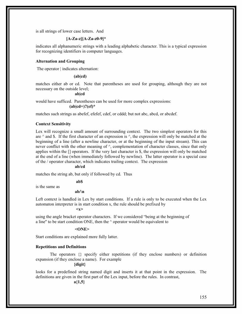
is all strings of lower case letters. And
[A-Za-z][A-Za-z0-9]*
indicates all alphanumeric strings with a leading alphabetic character. This is a typical expression for recognizing identifiers in computer languages.
Alternation and Grouping
The operator | indicates alternation:
(ab|cd)
matches either ab or cd. Note that parentheses are used for grouping, although they are not necessary on the outside level; ab|cd
would have sufficed. Parentheses can be used for more complex expressions: (ab|cd+)?(ef)*
matches such strings as abefef, efefef, cdef, or cddd; but not abc, abcd, or abcdef.
Context Sensitivity
Lex will recognize a small amount of surrounding context. The two simplest operators for this are ^ and $. If the first character of an expression is ^, the expression will only be matched at the beginning of a line (after a newline character, or at the beginning of the input stream). This can never conflict with the other meaning of ^, complementation of character classes, since that only applies within the [] operators. If the very last character is $, the expression will only be matched at the end of a line (when immediately followed by newline). The latter operator is a special case of the / operator character, which indicates trailing context. The expression ab/cd
matches the string ab, but only if followed by cd. Thus
ab$is the same as ab/\n
Left context is handled in Lex by start conditions. If a rule is only to be executed when the Lex automaton interpreter is in start condition x, the rule should be prefixed by <x>
using the angle bracket operator characters. If we considered “being at the beginning of a line'' to be start condition ONE, then the ^ operator would be equivalent to
<ONE>
Start conditions are explained more fully latter.
Repetitions and Definitions
The operators {} specify either repetitions (if they enclose numbers) or definition expansion (if they enclose a name). For example {digit}
looks for a predefined string named digit and inserts it at that point in the expression. The definitions are given in the first part of the Lex input, before the rules. In contrast, a{1,5}
155

looks for 1 to 5 occurrences of a.Finally, initial % is special, being the separator for Lex source segments.
The user will often want to know the actual text that matched some expression like [a-z]+. Lex leaves this text in an external character array named yytext. Thus, to printthe name found, a rule like
[a-z]+ printf("%s", yytext);
will print the string in yytext. The C function printf accepts a format argument and data to be printed; in this case, the format is “print string'' (% indicating data conversion, and %s indicating string type), and the data are the characters in yytext. So this just places the matched string on the output. This action is so common that it may be written as ECHO: [a-z]+ ECHO;
is the same as the above. Since the default action is just to print the characters found, one might ask why give a rule, like this one, which merely specifies the default action? Such rules are often required to avoid matching some other rule which is not desired. For example, if there is a rule which matches read it will normally match the instances of read contained in bread or readjust; to avoid this, a rule of the form [a-z]+ is needed. This is explained further below. Sometimes it is more convenient to know the end of what has been found; hence Lex also provides a count yyleng of the number of characters matched. To count both the number of words and the number of characters in words in the input, the user might write [a-zA-Z]+ {words++; chars += yyleng;}
which accumulates in chars the number of characters in the words recognized. The last character in the string matched can be accessed by yytext[yyleng-1]
Occasionally, a Lex action may decide that a rule has not recognized the correct span of characters. Two routines are provided to aid with this situation. First, yymore () can be called to indicate that the next input expression recognized is to be tacked on to the end of this input. Normally, the next input string would overwrite the current entry in yytext. Second, yyless (n) may be called to indicate that not all the characters matched by the currently successful expression are wanted right now. The argument n indicates the number of characters in yytext to be retained. Further characters previously matched are returned to the input. This provides the same sort of look ahead offered by the / operator, but in a different form. Example: Consider a language which defines a string as a set of characters between quotation (") marks, and provides that to include a "in a string it must be preceded by a \. The regular expression which matches that is somewhat confusing, so that it might be preferable to write \"[^"]* { if (yytext[yyleng-1] == '\\') yymore(); else ... normal user processing }
which will, when faced with a string such as "abc\" “def" first match the five characters "abc\”; then the call to yymore() will cause the next part of the string, "def, to be tacked on the end. Note that the final quote terminating the string should be picked up in the code labeled ``normal processing''.The function yyless () might be used to reprocess text in various circumstances. Consider the C problem of distinguishing the ambiguity of “=-a''. Suppose it is desired to treat this as “=- a'' but print a message. A rule might be
156

=-[a-zA-Z] { printf("Op (=-) ambiguous\n"); yyless(yyleng-1); ... action for =- ... }
which prints a message, returns the letter after the operator to the input stream, and treats the operator as ``=-''. Alternatively it might be desired to treat this as ``= -a''. To do this, just return the minus sign as well as the letter to the input: =-[a-zA-Z] { printf("Op (=-) ambiguous\n"); yyless(yyleng-2); ... action for = ... }
will perform the other interpretation. Note that the expressions for the two cases might more easily be written =-/[A-Za-z]
in the first case and =/-[A-Za-z]
in the second; no backup would be required in the rule action. It is not necessary to recognize the whole identifier to observe the ambiguity. The possibility of “=-3'', however, makes =-/[^ \t\n]
a still better rule. In addition to these routines, Lex also permits access to the I/O routines it uses.They are:
1) input() which returns the next input character;2) output(c) which writes the character c on the output; and3) unput(c) pushes the character c back onto the input stream to be read later by input().
By default these routines are provided as macro definitions, but the user can override them and supply private versions. These routines define the relationship between external files and internal characters, and must all be retained or modified consistently. They may be redefined, to cause input or output to be transmitted to or from strange places, including other programs or internal memory; but the character set used must be consistent in all routines; a value of zero returned by input must mean end of file; and the relationship between unput and input must be retained or the Lex lookahead will not work. Lex does not look ahead at all if it does not have to, but every rule ending in + * ? or $ or containing / implies lookahead. Lookahead is also necessary to match an expression that is a prefix of another expression. See below for a discussion of the character set used by Lex. The standard Lex library imposes a 100 character limit on backup. Another Lex library routine that the user will sometimes want to redefine is yywrap() which is called whenever Lex reaches an end-of-file. If yywrap returns a 1, Lex continues with the normal wrapup on end of input. Sometimes, however, it is convenient to arrange for more input to arrive from a new source. In this case, the user should provide a yywrap which arranges for new input and returns 0. This instructs Lex to continue processing. The default yywrap always returns 1.This routine is also a convenient place to print tables, summaries, etc. at the end of a program. Note that it is not possible to write a normal rule which recognizes end-of-file; the only access to this condition is through yywrap. In fact, unless a private version of input() is supplied a file containing nulls cannot be handled, since a value of 0 returned by input is taken to be end-of-file.
157

Ambiguous Source Rules Lex can handle ambiguous specifications. When more than one expression can match the
current input, Lex chooses as follows:
1) The longest match is preferred.2) Among rules which matched the same number of characters, the rule given first is
preferred. Thus, suppose the rules integer keyword action ...; [a-z]+ identifier action ...;
to be given in that order. If the input is integers, it is taken as an identifier, because [a-z]+ matches 8 characters while integer matches only 7. If the input is integer, both rules match 7 characters, and the keyword rule is selected because it was given first. Anything shorter (e.g. int) will not match the expression integer and so the identifier interpretation is used. The principle of preferring the longest match makes rules containing expressions like .* dangerous. For example, ' *'
might seem a good way of recognizing a string in single quotes. But it is an invitation for the program to read far ahead, looking for a distant single quote. Presented with the input 'first' quoted string here, 'second' here the above expression will match 'first' quoted string here, 'second' which is probably not what was wanted. A better rule is of the form '[^'\n]*'
which, on the above input, will stop after 'first'. The consequences of errors like this are mitigated by the fact that the . operator will not match newline. Thus expressions like .* stop on the current line. Don't try to defeat this with expressions like (.|\n)+ or equivalents; the Lex generated program will try to read the entire input file, causing internal buffer overflows.Note that Lex is normally partitioning the input stream, not searching for all possible matches of each expression. This means that each character is accounted for once and only once. For example, suppose it is desired to count occurrences of both she and he in an input text. Some Lex rules to do this might be she s++; he h++; \n | . ;
where the last two rules ignore everything besides he and she. Remember that . does not include newline. Since she includes he, Lex will normally not recognize the instances of he included in she, since once it has passed a she those characters are gone. Sometimes the user would like to override this choice. The action REJECT means ``go do the next alternative.'' It causes whatever rule was second choice after the current rule to be executed. The position of the input pointer is adjusted accordingly.Suppose the user really wants to count the included instances of he:
she {s++; REJECT;} he {h++; REJECT;} \n | . ;
these rules are one way of changing the previous example to do just that. After counting each expression, it is rejected; whenever appropriate, the other expression will then be counted. In this example, of course, the user could note that she includes he but not vice versa, and omit the
158
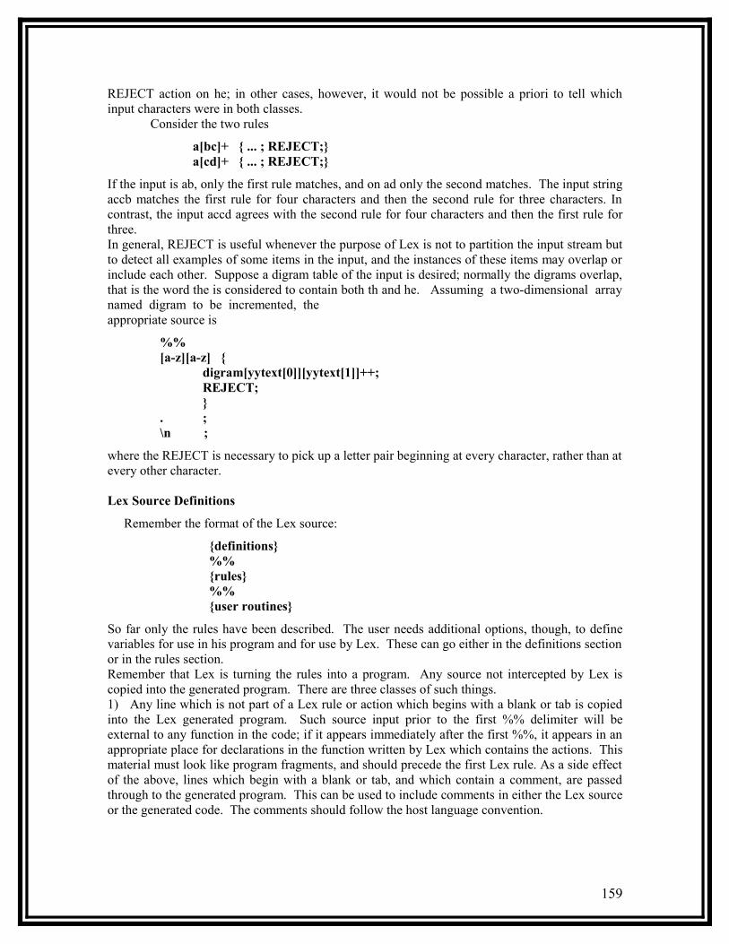
REJECT action on he; in other cases, however, it would not be possible a priori to tell which input characters were in both classes. Consider the two rules
a[bc]+ { ... ; REJECT;} a[cd]+ { ... ; REJECT;}
If the input is ab, only the first rule matches, and on ad only the second matches. The input string accb matches the first rule for four characters and then the second rule for three characters. In contrast, the input accd agrees with the second rule for four characters and then the first rule for three. In general, REJECT is useful whenever the purpose of Lex is not to partition the input stream but to detect all examples of some items in the input, and the instances of these items may overlap or include each other. Suppose a digram table of the input is desired; normally the digrams overlap, that is the word the is considered to contain both th and he. Assuming a two-dimensional array named digram to be incremented, theappropriate source is
%% [a-z][a-z] { digram[yytext[0]][yytext[1]]++; REJECT; } . ; \n ;
where the REJECT is necessary to pick up a letter pair beginning at every character, rather than at every other character.
Lex Source Definitions
Remember the format of the Lex source:
{definitions} %% {rules} %% {user routines}
So far only the rules have been described. The user needs additional options, though, to define variables for use in his program and for use by Lex. These can go either in the definitions section or in the rules section. Remember that Lex is turning the rules into a program. Any source not intercepted by Lex is copied into the generated program. There are three classes of such things. 1) Any line which is not part of a Lex rule or action which begins with a blank or tab is copied into the Lex generated program. Such source input prior to the first %% delimiter will be external to any function in the code; if it appears immediately after the first %%, it appears in an appropriate place for declarations in the function written by Lex which contains the actions. This material must look like program fragments, and should precede the first Lex rule. As a side effect of the above, lines which begin with a blank or tab, and which contain a comment, are passed through to the generated program. This can be used to include comments in either the Lex source or the generated code. The comments should follow the host language convention.
159
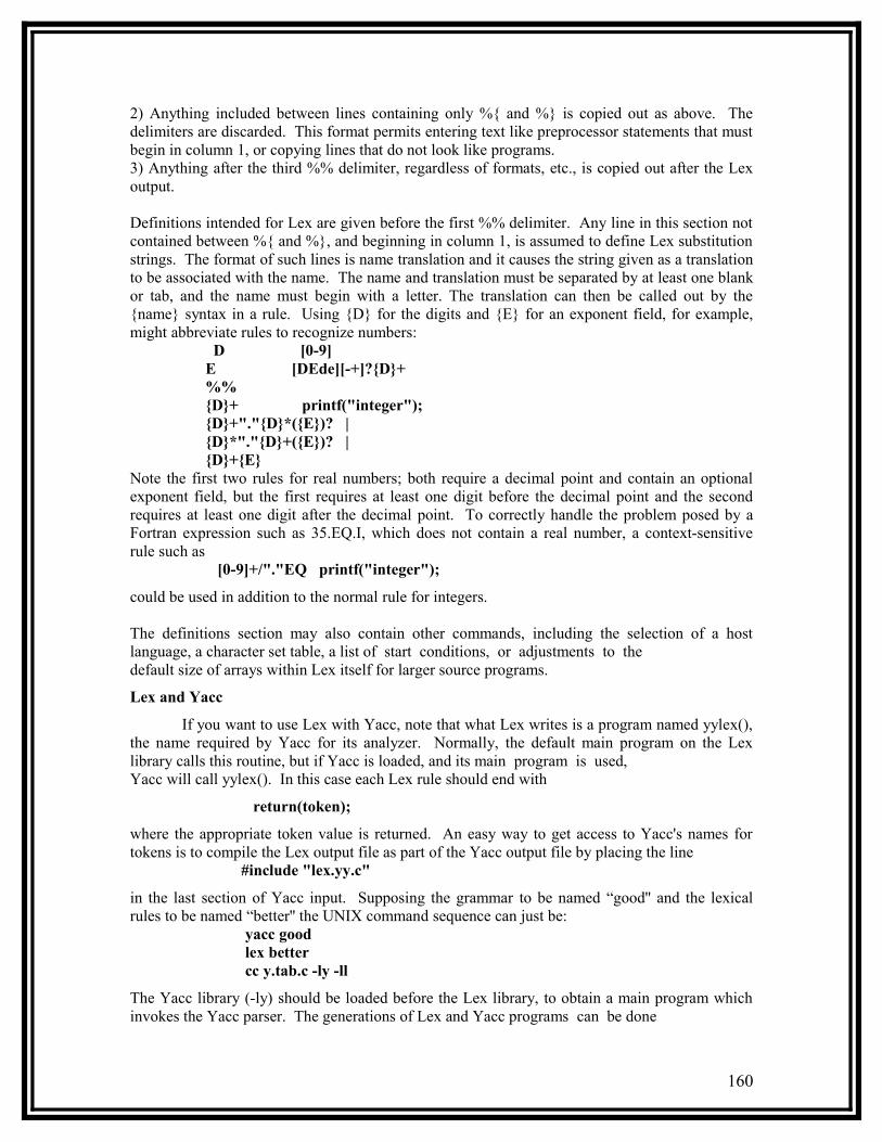
2) Anything included between lines containing only %{ and %} is copied out as above. The delimiters are discarded. This format permits entering text like preprocessor statements that must begin in column 1, or copying lines that do not look like programs.3) Anything after the third %% delimiter, regardless of formats, etc., is copied out after the Lex output.
Definitions intended for Lex are given before the first %% delimiter. Any line in this section not contained between %{ and %}, and beginning in column 1, is assumed to define Lex substitution strings. The format of such lines is name translation and it causes the string given as a translation to be associated with the name. The name and translation must be separated by at least one blank or tab, and the name must begin with a letter. The translation can then be called out by the {name} syntax in a rule. Using {D} for the digits and {E} for an exponent field, for example, might abbreviate rules to recognize numbers: D [0-9] E [DEde][-+]?{D}+ %% {D}+ printf("integer"); {D}+"."{D}*({E})? | {D}*"."{D}+({E})? | {D}+{E}Note the first two rules for real numbers; both require a decimal point and contain an optional exponent field, but the first requires at least one digit before the decimal point and the second requires at least one digit after the decimal point. To correctly handle the problem posed by a Fortran expression such as 35.EQ.I, which does not contain a real number, a context-sensitive rule such as [0-9]+/"."EQ printf("integer");
could be used in addition to the normal rule for integers.
The definitions section may also contain other commands, including the selection of a host language, a character set table, a list of start conditions, or adjustments to thedefault size of arrays within Lex itself for larger source programs.
Lex and Yacc
If you want to use Lex with Yacc, note that what Lex writes is a program named yylex(), the name required by Yacc for its analyzer. Normally, the default main program on the Lex library calls this routine, but if Yacc is loaded, and its main program is used,Yacc will call yylex(). In this case each Lex rule should end with
return(token);
where the appropriate token value is returned. An easy way to get access to Yacc's names for tokens is to compile the Lex output file as part of the Yacc output file by placing the line #include "lex.yy.c"
in the last section of Yacc input. Supposing the grammar to be named “good'' and the lexical rules to be named “better'' the UNIX command sequence can just be: yacc good lex better cc y.tab.c -ly -ll
The Yacc library (-ly) should be loaded before the Lex library, to obtain a main program which invokes the Yacc parser. The generations of Lex and Yacc programs can be done
160

in either order.
9.5 Examples
1. Write a Lex source program to copy an input file while adding 3 to every positive number divisible by 7. %% int k; [0-9]+ { k = atoi(yytext); if (k%7 == 0) printf("%d", k+3); else printf("%d",k); }to do just that. The rule [0-9]+ recognizes strings of digits; atoi converts the digits to binary and stores the result in k. The operator % (remainder) is used to check whether k is divisible by 7; if it is, it is incremented by 3 as it is written out. It may be objected that this program will alter such input items as 49.63 or X7. Furthermore, it increments the absolute value of all negative numbers divisible by 7. To avoid this, just add a few more rules after the active one, as here: %% int k; -?[0-9]+ { k = atoi(yytext); printf("%d", k%7 == 0 ? k+3 : k); } -?[0-9.]+ ECHO; [A-Za-z][A-Za-z0-9]+ ECHO;
Numerical strings containing a “.'' or preceded by a letter will be picked up by one of the last two rules, and not changed. The if-else has been replaced by a C conditional expression to save space; the form a?b:c means “if a then b else c''. 2. Write a Lex program that histograms the lengths of words, where a word is defined as a string of letters. int lengs[100]; %% [a-z]+ lengs[yyleng]++; . | \n ; %% yywrap() { int i; printf("Length No. words\n"); for(i=0; i<100; i++) if (lengs[i] > 0) printf("%5d%10d\n",i,lengs[i]); return(1); }
This program accumulates the histogram, while producing no output. At the end of the input it prints the table. The final statement return(1); indicates that Lex is to perform wrapup. If
161
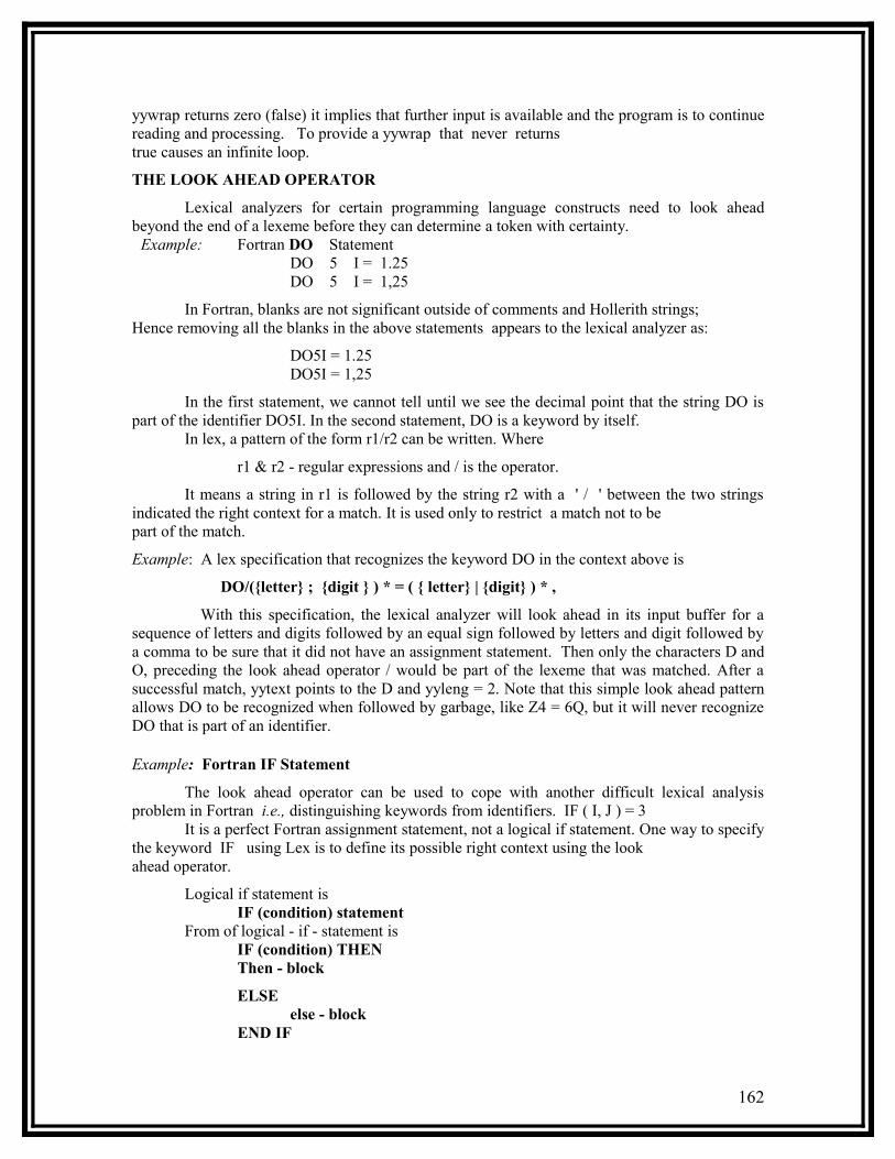
yywrap returns zero (false) it implies that further input is available and the program is to continue reading and processing. To provide a yywrap that never returnstrue causes an infinite loop.
THE LOOK AHEAD OPERATOR
Lexical analyzers for certain programming language constructs need to look ahead beyond the end of a lexeme before they can determine a token with certainty. Example: Fortran DO Statement
DO 5 I = 1.25DO 5 I = 1,25
In Fortran, blanks are not significant outside of comments and Hollerith strings; Hence removing all the blanks in the above statements appears to the lexical analyzer as:
DO5I = 1.25 DO5I = 1,25
In the first statement, we cannot tell until we see the decimal point that the string DO is part of the identifier DO5I. In the second statement, DO is a keyword by itself.
In lex, a pattern of the form r1/r2 can be written. Where
r1 & r2 - regular expressions and / is the operator.
It means a string in r1 is followed by the string r2 with a ' / ' between the two strings indicated the right context for a match. It is used only to restrict a match not to be part of the match.
Example: A lex specification that recognizes the keyword DO in the context above is
DO/({letter} ; {digit } ) * = ( { letter} | {digit} ) * ,
With this specification, the lexical analyzer will look ahead in its input buffer for a sequence of letters and digits followed by an equal sign followed by letters and digit followed by a comma to be sure that it did not have an assignment statement. Then only the characters D and O, preceding the look ahead operator / would be part of the lexeme that was matched. After a successful match, yytext points to the D and yyleng = 2. Note that this simple look ahead pattern allows DO to be recognized when followed by garbage, like Z4 = 6Q, but it will never recognize DO that is part of an identifier.
Example: Fortran IF Statement
The look ahead operator can be used to cope with another difficult lexical analysis problem in Fortran i.e., distinguishing keywords from identifiers. IF ( I, J ) = 3
It is a perfect Fortran assignment statement, not a logical if statement. One way to specify the keyword IF using Lex is to define its possible right context using the look ahead operator.
Logical if statement is IF (condition) statement
From of logical - if - statement isIF (condition) THENThen - block
ELSEelse - block
END IF
162

We note that every unlabeled Fortran statement begins with a letter and that every right parentheses used for subscripting or operand grouping must be followed by an operator symbol such as =, + or comma, another right parentheses or the end of the statement. A letter cannot follow such a right parentheses. In this situation, to confirm that IF is a keyword rather than an array name we scan forward looking for a right parentheses followed by a letter before seeing a new time character. This pattern for the keyword IF can be written as
IF / \ ( . * \ ) {letter}
The . (dot) stands for "any character but new line" and the back slashes in front of the parentheses till Lex to treat them literally, not as meta symbols for grouping in regular expressions.
The IF statements in Fortran can be solved by seeing IF ( . to determine whether IF has been declared an array. We scan for the full pattern indicated above if it has been so declared. Such texts makes the automatic implementation of a lexical analyzer from a Lex specification harder, and they may even cost time in the long run, since frequent checks must be made by the program simulating a transition diagram to determine whether any such tests must be made.
Programs: The lex programs are written in a file with a dot extension. Example first.l. The program is executed in the following manner:
% lex < filename.l >% cc lex.yy.c –o <execfilename> -ll
The lex translates the lex specification into a C source file called lex.yy.c which we compile with the lex library –ll. We then execute the resulting program to check that it works as we expect.
The exeution is as following:1. If –o <execfilename> is not given run the program by using ./a.out2. If –o<execfilename> is given run the program by using execfilename.3. Enter the data after execution.4. Use ^d to terminate the program and give result.
There are two programs written for the above requirement. The one is to give the text online after execution. When carriage return is pressed the yylex is executed and the printf statement is carried on displaying on the screen the total number of vowels and consonants.
This program is used to read the given text from a file. The file is opened in the read mode and the yylex function calls the base program to count the number of vowels and consonants. After it cover across the EOF, the C-program is executed to print the number of vowels and consonants. 1. Write a lex program to find the number of vowels and consonants.%{/* to find vowels and consonents*/ int vowels = 0; int consonents = 0;%}%%[ \t\n]+[aeiouAEIOU] vowels++;[bcdfghjklmnpqrstvwxyzBCDFGHJKLMNPQRSTVWXYZ] consonents++;. %%main(){
163

yylex(); printf(" The number of vowels = %d\n", vowels); printf(" number of consonents = %d \n", consonents);return(0);}
The same program can be executed by giving alternative grammar. It is as follows: Here a file is opened which is given as a argument and reads to text and counts the number of vowels and consonants.
%{ unsigned int vowelcount=0; unsigned int consocount=0;%}vowel [aeiouAEIOU]consonant [bcdfghjklmnpqrstvwxyzBCDFGHJKLMNPQRSTVWXYZ]eol \n%%{vowel} { vowelcount++;}{consonant} { consocount++; } %% main(int argc,char *argv[]){ if(argc > 1) { FILE *fp; fp=fopen(argv[1],"r"); if(!fp) { fprintf(stderr,"could not open %s\n",argv[1]); exit(1); } yyin=fp; } yylex(); printf(" vowelcount=%u consonantcount=%u\n ",vowelcount,consocount);return(0);}
2. Write a Lex program to count the number of words, characters, blanks and lines in a given text.
%{unsigned int charcount=0;
int wordcount=0; int linecount=0; int blankcount =0;%}word[^ \t\n]+eol \n%%[ ] blankcount++;{word} { wordcount++; charcount+=yyleng;}
164
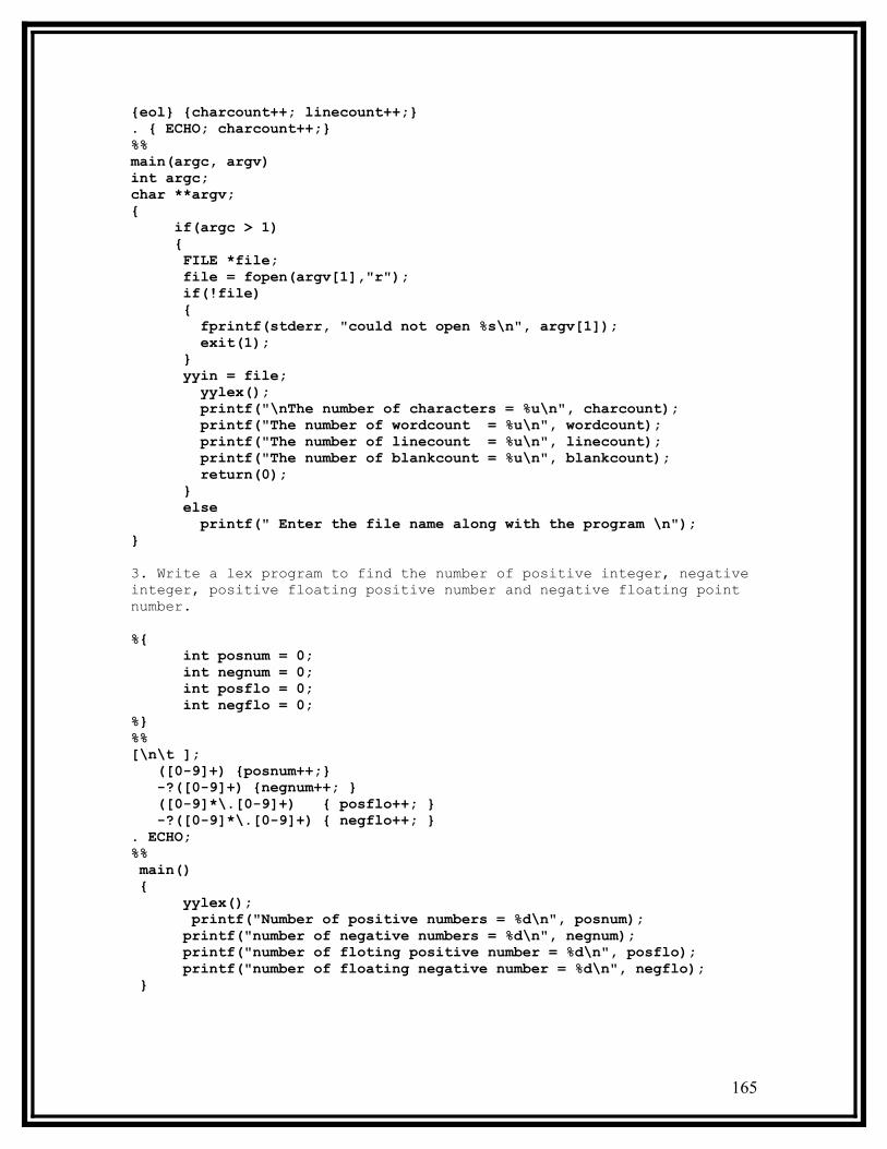
{eol} {charcount++; linecount++;}. { ECHO; charcount++;}%%main(argc, argv)int argc;char **argv;{ if(argc > 1) {
FILE *file;file = fopen(argv[1],"r");if(!file){ fprintf(stderr, "could not open %s\n", argv[1]); exit(1);}yyin = file;
yylex(); printf("\nThe number of characters = %u\n", charcount); printf("The number of wordcount = %u\n", wordcount); printf("The number of linecount = %u\n", linecount); printf("The number of blankcount = %u\n", blankcount); return(0); } else printf(" Enter the file name along with the program \n");}3. Write a lex program to find the number of positive integer, negative integer, positive floating positive number and negative floating point number.
%{int posnum = 0;int negnum = 0;
int posflo = 0; int negflo = 0;%}%%[\n\t ]; ([0-9]+) {posnum++;} -?([0-9]+) {negnum++; } ([0-9]*\.[0-9]+) { posflo++; } -?([0-9]*\.[0-9]+) { negflo++; } . ECHO; %% main() {
yylex(); printf("Number of positive numbers = %d\n", posnum); printf("number of negative numbers = %d\n", negnum);
printf("number of floting positive number = %d\n", posflo);printf("number of floating negative number = %d\n", negflo);
}
165

4. Write a lex program to find the given c program has right number of brackets. Count the number of comments. Check for while loop.
%{ /* find main, comments, {, (, ), } */ int comments=0; int opbr=0; int clbr=0; int opfl=0; int clfl=0; int j=0; int k=0;%}%%"main()" j=1;"/*"[ \t].*[ \t]"*/" comments++;"while("[0-9a-zA-Z]*")"[ \t]*\n"{"[ \t]*.*"}" k=1;^[ \t]*"{"[ \t]*\n^[ \t]*"}" k=1;"(" opbr++;")" clbr++;"{" opfl++; "}" clfl++;[^ \t\n]+. ECHO;%%main(argc, argv)int argc;char *argv[];{ if (argc > 1) { FILE *file; file = fopen(argv[1], "r"); if (!file) {
printf("error opeing a file \n"); exit(1); } yyin = file; } yylex(); if(opbr != clbr) printf("open brackets is not equal to close brackets\n"); if(opfl != clfl)
printf("open flower brackets is not equal to close flower brackets\n");
printf(" the number of comments = %d\n",comments); if (!j) printf("there is no main function \n"); if (k) printf("there is loop\n"); else printf("there is no valid for loop\n"); return(0);}
166

5. Write a lex program to replace scanf with READ and printf with WRITE statement also find the number of scanf and printf.
%{int pc=0,sc=0;%}%%printf fprintf(yyout,"WRITE");pc++;scanf fprintf(yyout,"READ");sc++;. ECHO;%%main(int argc,char* argv[]){ if(argc!=3) { printf("\nUsage: %s <src> <dest>\n",argv[0]); return; } yyin=fopen(argv[1],"r"); yyout=fopen(argv[2],"w"); yylex(); printf("\nno. of printfs:%d\nno. of scanfs:%d\n",pc,sc);}6. Write a lex program to find whether the given expression is valid.
%{ #include <stdio.h> int valid=0,ctr=0,oc = 0;%}NUM [0-9]+OP [+*/-]%%{NUM}({OP}{NUM})+ { valid = 1; for(ctr = 0;yytext[ctr];ctr++)
{ switch(yytext[ctr]) { case '+':
case '-': case '*': case '/': oc++;
} }
}{NUM}\n {printf("\nOnly a number.");}\n { if(valid) printf("valid \n operatorcount = %d",oc); else printf("Invalid"); valid = oc = 0;ctr=0; } %%main(){ yylex();}
167

/* Another solution for the same problem */%{int oprc=0,digc=0,top=-1,flag=0;char stack[20];%}digit [0-9]+opr [+*/-]%%[ \n\t]+['('] {stack[++top]='(';}[')'] {flag=1; if(stack[top]=='('&&(top!=-1))
top--; else
{printf("\n Invalid expression\n"); exit(0);}
}{digit} {digc++;}{opr}/['('] { oprc++; printf("%s",yytext);}{opr}/{digit} {oprc++; printf("%s",yytext);}. {printf("Invalid "); exit(0);}%%main(){yylex();if((digc==oprc+1||digc==oprc) && top==-1){ printf("VALID");printf("\n oprc=%d\n digc=%d\n",oprc,digc);}elseprintf("INVALID");}
7.Write a lex program to find the given sentence is simple or compound.%{int flag=0;%}%%(" "[aA][nN][dD]" ")|(" "[oO][rR]" ")|(" "[bB][uU][tT]" ") flag=1;. ;%%main(){yylex();if (flag==1)
printf("COMPOUND SENTENCE \n");else
printf("SIMPLE SENTENCE \n");}8. Write a lex program to find the number of valid identifiers.
%{
168

int count=0;%}%%(" int ")|(" float ")|(" double ")|(" char ") {int ch; ch = input();for(;;) { if (ch==',') {count++;} else
if(ch==';') {break;} ch = input();
} count++;}%%main(int argc,char *argv[]){yyin=fopen(argv[1],"r");yylex();printf("the no of identifiers used is %d\n",count);}
Exercises
1. How is Lexical analyzer created with Lex?2. How does Lex behave in concert with aparser?3. Why should the lex select the longest prefix match pattern?4. Why should lexical analyzer need to llo ahead to determine a token?5. Explain how the lexical analyzer will recognize IF statement in FOTRAN?
169
YACC
Introduction
Yacc provides a general tool for describing the input to a computer program. The Yacc user specifies the structures of his input, together with code to be invoked as each such structure is recognized. Yacc turns such a specification into a subroutine that handles the input process; frequently, it is convenient and appropriate to have most of the flow of control in the user's application handled by this subroutine.
The input subroutine produced by Yacc calls a user-supplied routine to return the next basic input item. Thus, the user can specify his input in terms of individual input characters or in terms of higher level constructs such as names and numbers. The user supplied routine may also handle idiomatic features such as comment and continuation conventions, which typically defy easy grammatical specification. Yacc is written in portable C.
Yacc provides a general tool for imposing structure on the input to a computer program. User prepares a specification of the input process; this includes rules describing the input structure, code to be invoked when these rules are recognized, and a low-level routine to do the basic input. Yacc then generates a function to control the input process. This function, called a parser, calls the user-supplied low-level input routine (the lexical analyzer) to pick up the basic items (called tokens) from the input stream. These tokens are organized according to the input structure rules, called grammar rules; when one of these rules has been recognized, then user code supplied for this rule, an action, is invoked; actions have the ability to return values and make use of the values of other actions. Yacc is written in a portable dialect of C and the actions, and output subroutine, are in C as well. Moreover, many of the syntactic conventions of Yacc follow C. The heart of the input specification is a collection of grammar rules. Each rule describes an allowable structure and gives it a name. For example, one grammar rule might be date : month_name day ',' year
Here, date, month_name, day, and year represent structures of interest in the input process; presumably, month_name, day, and year are defined elsewhere. The comma ``,'' is enclosed in single quotes; this implies that the comma is to appear literally in the input. The colon and semicolon merely serve as punctuation in the rule, and have no significance in controlling the input. Thus, with proper definitions, the input
July 4, 1776
might be matched by the above rule.
An important part of the input process is carried out by the lexical analyzer. This user routine reads the input stream, recognizing the lower level structures, and communicates these tokens to the parser. For historical reasons, a structure recognized by the lexical analyzer is called a terminal symbol, while the structure recognized by the parser is called a nonterminal symbol. To avoid confusion, terminal symbols will usually be referred to as tokens.
170
There is considerable leeway (flexibility) in deciding whether to recognize structures using the lexical analyzer or grammar rules. For example, the rules month_name : 'J' 'a' 'n' ; month_name : 'F' 'e' 'b' ; . . . month_name : 'D' 'e' 'c' ;
might be used in the above example. The lexical analyzer would only need to recognize individual letters, and month_name would be a nonterminal symbol. Such low-level rules tend to waste time and space, and may complicate the specification beyond Yacc's ability to deal with it. Usually, the lexical analyzer would recognize the month names, and return an indication that a month_name was seen; in this case, month_name would be a token.
Literal characters such as ``,'' must also be passed through the lexical analyzer, and are also considered tokens. Specification files are very flexible. It is relatively easy to add to the above example the rule date: month '/' day '/' year; allowing 7 / 4 / 1776 as a synonym for July 4, 1776. In most cases, this new rule could be ``slipped in'' to a working system with minimal effort, and little danger of disrupting existing input. The input being read may not conform to the specifications. These input errors are detected as early as is theoretically possible with a left-to-right scan; thus, not only is the chance of reading and computing with bad input data substantially reduced, but the bad data can usually be quickly found. Error handling, provided as part of the input specifications, permits the reentry of bad data, or the continuation of the input process after skipping over the bad data. In some cases, Yacc fails to produce a parser when given a set of specifications. For example, the specifications may be self contradictory, or they may require a more powerful recognition mechanism than that available to Yacc. The former cases represent design errors; the latter cases can often be corrected by making the lexical analyzer more powerful, or by rewriting some of the grammar rules. While Yacc cannot handle all possible specifications, its power compares favorably with similar systems; moreover, the constructions which are difficult for Yacc to handle are also frequently difficult for human beings to handle. Some users have reported that the discipline of formulating valid Yacc specifications for their input revealed errors of conception or design early in the program development.
1. Basic Specifications
Every specification file consists of three sections: the declarations, (grammar) rules, and programs. The sections are separated by double percent ``%%'' marks. (The percent ``%'' is generally used in Yacc specifications as an escape character.)
In other words, a full specification file looks like declarations %% rules %% programs
171
The declaration section may be empty. Moreover, if the programs section is omitted, the second %% mark may be omitted also; thus, the smallest legal Yacc specification is %% rules
Blanks, tabs, and newlines are ignored except that they may not appear in names or multi-character reserved symbols. Comments may appear wherever a name is legal; they are enclosed in /* . . . */, as in C and PL/I.
The rules section is made up of one or more grammar rules.A grammar rule has the form: A : BODY ;A represents a nonterminal name, and BODY represents a sequence of zero or more names and literals. The colon and the semicolon are Yacc punctuation.
Names may be of arbitrary length, and may be made up of letters, dot ``.'', underscore ``_'', and non-initial digits. Upper and lower case letters are distinct. The names used in the body of a grammar rule may represent tokens or nonterminal symbols. A literal consists of a character enclosed in single quotes ``'''. As in C, the backslash ``\'' is an escape character within literals, and all the C escapes are recognized. Thus '\n' newline '\r' return '\'' single quote ``''' '\\' backslash ``\'' '\t' tab '\b' backspace '\f' form feed '\xxx' ``xxx'' in octalFor a number of technical reasons, the NUL character ('\0' or 0) should never be used in grammar rules.
If there are several grammar rules with the same left hand side, the vertical bar ``|'' can be used to avoid rewriting the left hand side. In addition, the semicolon at the end of a rule can be dropped before a vertical bar. Thus the grammar rules A : B C D ; A : E F ; A : G ;can be given to Yacc as A : B C D | E F | G ;
It is not necessary that all grammar rules with the same left side appear together in the grammar rules section, although it makes the input much more readable, and easier to change. If a nonterminal symbol matches the empty string, this can be indicated in the obvious way: empty : ;
Names representing tokens must be declared; this is most simply done by writing %token name1, name2 . . .
172

in the declarations section. Every name not defined in the declarations section is assumed to represent a non-terminal symbol. Every non-terminal symbol must appear on the left side of at least one rule. Of all the nonterminal symbols, one, called the start symbol, has particular importance. The parser is designed to recognize the start symbol; thus, this symbol represents the largest, most general structure described by the grammar rules. By default, the start symbol is taken to be the left hand side of the first grammar rule in the rules section. It is possible, and in fact desirable, to declare the start symbol explicitly in the declarations section using the % start keyword:
%start symbol
The end of the input to the parser is signaled by a special token, called the endmarker. If the tokens up to, but not including, the endmarker form a structure which matches the start symbol, the parser function returns to its caller after the end-marker is seen; it accepts the input. If the endmarker is seen in any other context, it is an error.
It is the job of the user-supplied lexical analyzer to return the endmarker when appropriate; see section 3, below. Usually the endmarker represents some reasonably obvious I/O status, such as ``end-of-file'' or ``end-of-record''.
2: Actions: With each grammar rule, the user may associate actions to be Yacc: Yet Another Compiler-Compiler performed each time the rule is recognized in the input process. These actions may return values, and may obtain the values returned by previous actions. Moreover, the lexical analyzer can return values for tokens, if desired.An action is an arbitrary C statement, and as such can do input and output, call subprograms, and alter external vectors and variables. An action is specified by one or more statements, enclosed in curly braces ``{'' and ``}''. For example,
A : '(' B ')' { hello( 1, "abc" ); }and XXX : YYY ZZZ { printf("a message\n"); flag = 25; }
are grammar rules with actions.
To facilitate easy communication between the actions and the parser, the action statements are altered slightly. The symbol ``dollar sign'' ``$'' is used as a signal to Yacc in this context.
To return a value, the action normally sets the pseudo-variable ``$$'' to some value. For example, an action that does nothing but return the value 1 is
{ $$ = 1; }
To obtain the values returned by previous actions and the lexical analyzer, the action may use the pseudo-variables $1, $2, . . ., which refer to the values returned by the components of the right side of a rule, reading from left to right. Thus, if the rule is
173

A : B C D ;
for example, then $2 has the value returned by C, and $3 the value returned by D. As a more concrete example, consider the rule
expr : '(' expr ')' ;The value returned by this rule is usually the value of the expr in parentheses. This can
be indicated by expr : '(' expr ')' { $$ = $2 ; }
By default, the value of a rule is the value of the first element in it ($1). Thus, grammar rules of the form A : B ;
frequently need not have an explicit action. In the examples above, all the actions came at the end of their rules. Sometimes, it is desirable to get control before a rule is fully parsed. Yacc permits an action to be written in the middle of a rule as well as at the end. This rule is assumed to return a value, accessible through the usual mechanism by the actions to the right of it. In turn, it may access the values returned by the symbols to its left. Thus, in the rule A : B { $$ = 1; } C { x = $2; y = $3; } ;the effect is to set x to 1, and y to the value returned by C. Actions that do not terminate a rule are actually handled by Yacc by manufacturing a new nonterminal symbol name, and a new rule matching this name to the empty string. The interior action is the action triggered off by recognizing this added rule. Yacc actually treats the above example as if it had been written:
$ACT : /* empty */ { $$ = 1; } ;
A : B $ACT C { x = $2; y = $3; } ;
In many applications, output is not done directly by the actions; rather, a data structure, such as a parse tree, is constructed in memory, and transformations are applied to it before output is generated. Parse trees are particularly easy to construct, given routines to build and maintain the tree structure desired. For example, suppose there is a C function node, written so that the call node( L, n1, n2 )
creates a node with label L, and descendants n1 and n2, and returns the index of the newly created node. Then parse tree can be built by supplying actions such as: expr : expr '+' expr { $$ = node( '+', $1, $3 ); }
in the specification.
The user may define other variables to be used by the actions. Declarations and definitions can appear in the declarations section, enclosed in the marks ``%{'' and ``%}''. These
174

declarations and definitions have global scope, so they are known to the action statements and the lexical analyzer. For example,
%{ int variable = 0; %}
could be placed in the declarations section, making variable accessible to all of the actions. The Yacc parser uses only names beginning in ``yy''; the user should avoid such names.In these examples, all the values are integers: a discussion of values of other types will be found in Section 10.
3: Lexical Analysis
The user must supply a lexical analyzer to read the input stream and communicate tokens (with values, if desired) to the parser. The lexical analyzer is an integer-valued function called yylex. The user must supply a lexical analyzer to read the input stream and communicate tokens (with values, if desired) to the parser. The lexical analyzer is an integer-valued function called yylex. The parser and the lexical analyzer must agree on these token numbers in order for communication between them to take place. The numbers may be chosen by Yacc, or chosen by the user. In either case, the ``# define'' mechanism of C is used to allow the lexical analyzer to return these numbers symbolically. For example, suppose that the token name DIGIT has been defined in the declarations section of the Yacc specification file. The relevant portion of the lexical analyzer might look like:
yylex(){ extern int yylval; int c; . . . c = getchar(); . . . switch( c ) { . . . case '0': case '1': . . . case '9': yylval = c-'0'; return( DIGIT ); . . . } . . .
The intent is to return a token number of DIGIT, and a value equal to the numerical value of the digit. Provided that the lexical analyzer code is placed in the programs section of the specification file, the identifier DIGIT will be defined as the token number associated with the token DIGIT.
This mechanism leads to clear, easily modified lexical analyzers; the only pitfall is the need to avoid using any token names in the grammar that are reserved or significant in C or the parser; for example, the use of token names ‘if’ or ‘while’ will almost certainly cause severe difficulties when the lexical analyzer is compiled. The token name error is reserved for error handling, and should not be used naively.
175

As mentioned above, the token numbers may be chosen by Yacc or by the user. In the default situation, the numbers are chosen by Yacc. The default token number for a literal character is the numerical value of the character in the local character set. Other names are assigned token numbers starting at 257.
To assign a token number to a token (including literals), the first appearance of the token name or literal in the declarations section can be immediately followed by a nonnegative integer. This integer is taken to be the token number of the name or literal. Names and literals not defined by this mechanism retain their default definition. It is important that all token numbers be distinct.
For historical reasons, the end marker must have token number 0 or negative. This token number cannot be redefined by the user; thus, all lexical analyzers should be prepared to return 0 or negative as a token number upon reaching the end of their input. A very useful tool for constructing lexical analyzers is the Lex program developed by Mike Lesk.[8] These lexical analyzers are designed to work in close harmony with Yacc parsers. The specifications for these lexical analyzers use regular expressions instead of grammar rules. Lex can be easily used to produce quite complicated lexical analyzers, but there remain some languages (such as FORTRAN) which do not fit any theoretical framework, and whose lexical analyzers must be crafted by hand.
4: How the Parser Works
Yacc turns the specification file into a C program, which parses the input according to the specification given. The algorithm used to go from the specification to the parser is complex, and will not be discussed here (see the references for more information). The parser itself, however, is relatively simple, and understanding how it works, while not strictly necessary, will nevertheless make treatment of error recovery and ambiguities much more comprehensible.
The parser produced by Yacc consists of a finite state machine with a stack. The parser is also capable of reading and remembering the next input token (called the lookahead token). The current state is always the one on the top of the stack. The states of the finite state machine are given small integer labels; initially, the machine is in state 0, the stack contains only state 0, and no lookahead token has been read.
The machine has only four actions available to it, called shift, reduce, accept, and error. A move of the parser is done as follows:
1. Based on its current state, the parser decides whether it needs a lookahead token to decide what action should be done; if it needs one, and does not have one, it calls yylex to obtain the next token. 2. Using the current state, and the lookahead token if needed, the parser decides on its next action, and carries it out. This may result in states being pushed onto the stack, or popped off the stack, and in the lookahead token being processed or left alone. The shift action is the most common action the parser takes. Whenever a shift action is taken, there is always a lookahead token. For example, in state 56 there may be an action:
IF shift 34
176
which says, in state 56, if the lookahead token is IF, the current state (56) is pushed down on the stack, and state 34 becomes the current state (on the top of the stack). The look ahead token is cleared. The reduce action keeps the stack from growing without bounds. Reduce actions are appropriate when the parser has seen the right hand side of a grammar rule, and is prepared to announce that it has seen an instance of the rule, replacing the right hand side by the left hand side. It may be necessary to consult the lookahead token to decide whether to reduce, but usually it is not; in fact, the default action (represented by a ``.'') is often a reduce action. Reduce actions are associated with individual grammar rules. Grammar rules are also given small integer numbers, leading to some confusion. The action
. reduce 18
refers to grammar rule 18, while the action IF shift 34refers to state 34. Suppose the rule being reduced is A : x y z ;
The reduce action depends on the left hand symbol (A in this case), and the number of symbols on the right hand side (three in this case). To reduce, first pop off the top three states from the stack (In general, the number of states popped equals the number of symbols on the right side of the rule). In effect, these states were the ones put on the stack while recognizing x, y, and z, and no longer serve any useful purpose. After popping these states, a state is uncovered which was the state the parser was in before beginning to process the rule. Using this uncovered state, and the symbol on the left side of the rule, perform what is in effect a shift of A. A new state is obtained, pushed onto the stack, and parsing continues. There are significant differences between the processing of the left hand symbol and an ordinary shift of a token, however, so this action is called a goto action. In particular, the lookahead token iscleared by a shift, and is not affected by a goto. In any case, the uncovered state contains an entry such as: A goto 20
causing state 20 to be pushed onto the stack, and become the current state. n effect, the reduce action ``turns back the clock'' in the parse, popping the states off the stack to go back to the state where the right hand side of the rule was first seen. The parser then behaves as if it had seen the left side at that time. If the right hand side of the rule is empty, no states are popped off of the stack: the uncovered state is in fact the current state. The reduce action is also important in the treatment of user-supplied actions and values. When a rule is reduced, the code supplied with the rule is executed before the stack is adjusted. In addition to the stack holding the states, another stack, running in parallel with it, holds the values returned from the lexical analyzer and the actions. When a shift takes place, the external variable yylval is copied onto the value stack. After the return from the user code, the reduction is carried out. When the goto action is done, the external variable yyval is copied onto the value stack. The pseudo-variables $1, $2, etc., refer to the value stack. The other two parser actions are conceptually much simpler. The accept action indicates that the entire input has been seen and that it matches the specification. This action appears only when the lookahead token is the endmarker, and indicates that the parser has successfully done its job. The error action, on the other hand, represents a place where the parser can no longer continue parsing according to the specification. The input tokens it has seen, together with the lookahead token, cannot be followed by anything that would result in a legal input. The parser reports an error, and attempts to recover the situation and resume parsing: the error recovery (as opposed to the detection of error).
177

Example1: Consider the specification
%token DING DONG DELL %% rhyme : sound place ; sound : DING DONG ; place : DELL ;
When Yacc is invoked with the -v option, a file called y.output is produced, with a human-readable description of the parser. The y.output file corresponding to the above grammar (with some statistics stripped off the end) is:
state 0 $accept : _rhyme $end DING shift 3 . error rhyme goto 1 sound goto 2
state 1 $accept : rhyme_$end $end accept . error state 2 rhyme : sound_place DELL shift 5 . error place goto 4 state 3 sound : DING_DONG DONG shift 6 . error state 4 rhyme : sound place_ (1) . reduce 1 state 5 place : DELL_ (3) . reduce 3 state 6 sound : DING DONG_ (2) . reduce 2
Notice that, in addition to the actions for each state, there is a description of the parsing rules being processed in each state. The _ character is used to indicate what has been seen, and what is yet to come, in each rule. Suppose the input is DING DONG DELL. It is instructive to follow the steps of the parser while processing this input.
178
nitially, the current state is state 0. The parser needs to refer to the input in order to decide between the actions available in state 0, so the first token, DING, is read, becoming the lookahead token. The action in state 0 on DING is is ``shift 3'', so state 3 is pushed onto the stack, and the lookahead token is cleared. State 3 becomes the current state. The next token, DONG, is read, becoming the lookahead token. The action in state 3 on the token DONG is ``shift 6'', so state 6 is pushed onto the stack, and the lookahead is cleared. The stack now contains 0, 3, and 6. In state 6, without even consulting the lookahead, the parser reduces by rule 2. sound : DING DONG
This rule has two symbols on the right hand side, so two states, 6 and 3, are popped off of the stack, uncovering state 0. Consulting the description of state 0, looking for a goto on sound, sound goto 2
is obtained; thus state 2 is pushed onto the stack, becoming the current state. In state 2, the next token, DELL, must be read. The action is ``shift 5'', so state 5 is pushed onto the stack, which now has 0, 2, and 5 on it, and the lookahead token is cleared. In state 5, the only action is to reduce by rule 3. This has one symbol on the right hand side, so one state, 5, is popped off, and state 2 is uncovered. The goto in state 2 on place, the left side of rule 3, is state 4. Now, the stack contains 0, 2, and 4. In state 4, the only action is to reduce by rule 1. There are two symbols on the right, so the top two states are popped off, uncovering state 0 again. In state 0, there is a goto on rhyme causing the parser to enter state 1. In state 1, the input is read; the endmarker is obtained, indicated by ``$end'' in the y.output file. The action in state 1 when the endmarker is seen is to accept, successfully ending the parse. The reader is urged to consider how the parser works when confronted with such incorrect strings as DING DONG DONG, DING DONG, DING DONG DELL DELL, etc. A few minutes spend with this and other simple examples will probably be repaid when problems arise in more complicated contexts.
5: Ambiguity and Conflicts A set of grammar rules is ambiguous if there is some input string that can be structured in two or more different ways. For example, the grammar rule
expr : expr '-' expr
is a natural way of expressing the fact that one way of forming an arithmetic expression is to put two other expressions together with a minus sign between them. Unfortunately, this grammar rule does not completely specify the way that all complex inputs should be structured. For example, if the input is expr - expr - expr
the rule allows this input to be structured as either ( expr - expr ) - expr
or as
expr - ( expr - expr )
(The first is called left association, the second right association). Yacc detects such ambiguities when it is attempting to build the parser. It is instructive to consider the problem that confronts the parser when it is given an input such as
179

expr - expr - expr
When the parser has read the second expr, the input that it has seen:
expr - expr
matches the right side of the grammar rule above. The parser could reduce the input by applying this rule; after applying the rule; the input is reduced to expr (the left side of the rule). The parser would then read the final part of the input:
- expr
and again reduce. The effect of this is to take the left associative interpretation. Alternatively, when the parser has seen expr - expr
it could defer the immediate application of the rule, and continue reading the input until it had seen expr - expr - expr
It could then apply the rule to the rightmost three symbols, reducing them to expr and leaving expr - expr
Now the rule can be reduced once more; the effect is to take the right associative interpretation. Thus, having read
expr - expr
the parser can do two legal things, a shift or a reduction, and has no way of deciding between them. This is called a shift / reduce conflict. It may also happen that the parser has a choice of two legal reductions; this is called a reduce / reduce conflict. Note that there are never any ``Shift/shift'' conflicts. When there are shift/reduce or reduce/reduce conflicts, Yacc still produces a parser. It does this by selecting one of the valid steps wherever it has a choice. A rule describing which choice to make in a given situation is called a disambiguating rule.
Yacc invokes two disambiguating rules by default:
1. In a shift/reduce conflict, the default is to do the shift.
2. In a reduce/reduce conflict, the default is to reduce by the earlier grammar rule (in the input sequence). Rule 1 implies that reductions are deferred whenever there is a choice, in favor of shifts. Rule 2 gives the user rather crude control over the behavior of the parser in this situation, but reduce/reduce conflicts should be avoided whenever possible. Conflicts may arise because of mistakes in input or logic, or because the grammar rules, while consistent, require a more complex parser than Yacc can construct. The use of actions within rules can also cause conflicts, if the action must be done before the parser can be sure which rule is being recognized. In these cases, the application of disambiguating rules is inappropriate, and leads to an incorrect parser. For this reason, Yacc always reports the number of shift/reduce and reduce/reduce conflicts resolved by Rule 1 and Rule 2.
180
In general, whenever it is possible to apply disambiguating rules to produce a correct parser, it is also possible to rewrite the grammar rules so that the same inputs are read but there are no conflicts. For this reason, most previous parser generators have considered conflicts to be fatal errors. Our experience has suggested that this rewriting is somewhat unnatural, and produces slower parsers; thus, Yacc will produce parsers even in the presence of conflicts. As an example of the power of disambiguating rules, consider a fragment from a programming language involving an ``if-then-else'' construction:
stat : IF '(' cond ')' stat | IF '(' cond ')' stat ELSE stat ;
In these rules, IF and ELSE are tokens, cond is a nonterminal symbol describing conditional (logical) expressions, and stat is a nonterminal symbol describing statements. The first rule will be called the simple-if rule, and the second the if-else rule. These two rules form an ambiguous construction, since input of the form
IF ( C1 ) IF ( C2 ) S1 ELSE S2
can be structured according to these rules in two ways:
IF ( C1 ) { IF ( C2 ) S1 } ELSE S2
or
IF ( C1 ) { IF ( C2 ) S1 ELSE S2 }
The second interpretation is the one given in most programming languages having this construct. Each ELSE is associated with the last preceding ``un-ELSE'd'' IF. In this example, consider the situation where the parser has seen
IF ( C1 ) IF ( C2 ) S1
and is looking at the ELSE. It can immediately reduce by the simple-if rule to get
IF ( C1 ) statand then read the remaining input, ELSE S2and reduce IF ( C1 ) stat ELSE S2by the if-else rule. This leads to the first of the above groupings of the input. On the other hand, the ELSE may be shifted, S2 read, and then the right hand portion of IF ( C1 ) IF ( C2 ) S1 ELSE S2can be reduced by the if-else rule to get
IF ( C1 ) stat
181

which can be reduced by the simple-if rule. This leads to the second of the above groupings of the input, which is usually desired. Once again the parser can do two valid things - there is a shift/reduce conflict. The application of disambiguating rule 1 tells the parser to shift in this case, which leads to the desired grouping. This shift/reduce conflict arises only when there is a particular current input symbol, ELSE, and particular inputs already seen, such as IF ( C1 ) IF ( C2 ) S1In general, there may be many conflicts, and each one will be associated with an input symbol and a set of previously read inputs. The previously read inputs are characterized by the state of the parser. The conflict messages of Yacc are best understood by examining the verbose (-v) option output file. For example, the output corresponding to the above conflict state might be: 23: shift/reduce conflict (shift 45, reduce 18) on ELSE state 23 stat : IF ( cond ) stat_ (18) stat : IF ( cond ) stat_ELSE stat ELSE shift 45 . reduce 18The first line describes the conflict, giving the state and the input symbol. The ordinary state description follows, giving the grammar rules active in the state, and the parser actions. Recall that the underline marks the portion of the grammar rules which has been seen. Thus in the example, in state 23 the parser has seen input corresponding to IF ( cond ) statand the two grammar rules shown are active at this time. The parser can do two possible things. If the input symbol is ELSE, it is possible to shift into state 45. State 45 will have, as part of its description, the line stat : IF ( cond ) stat ELSE_statsince the ELSE will have been shifted in this state. Back in state 23, the alternative action, described by ``.'', is to be done if the input symbol is not mentioned explicitly in the above actions; thus, in this case, if the input symbol is not ELSE, the parser reduces by grammar rule 18:
stat : IF '(' cond ')' statOnce again, notice that the numbers following ``shift'' commands refer to other states, while the numbers following ``reduce'' commands refer to grammar rule numbers. In the y.output file, the rule numbers are printed after those rules which can be reduced. In most one states, there will be at most reduce action possible in the state, and this will be the default command. The user who encounters unexpected shift/reduce conflicts will probably want to look at the verbose output to decide whether the default actions are appropriate. In really tough cases, the user might need to know more about the behavior and construction of the parser than can be covered here. In this case, one of the theoretical references[2, 3, 4] might be consulted; the services of a local guru might also be appropriate.6: Precedence There is one common situation where the rules given above for resolving conflicts are not sufficient; this is in the parsing of arithmetic expressions. Most of the commonly used constructions for arithmetic expressions can be naturally described by the notion of precedence levels for operators, together with information about left or right associatively. It turns out that ambiguous grammars with appropriate disambiguating rules can be used to create parsers that are faster and easier to write than parsers constructed from unambiguous grammars. The basic notion is to write grammar rules of the form expr : expr OP expr
182

and expr : UNARY exprfor all binary and unary operators desired. This creates a very ambiguous grammar, with many parsing conflicts. As disambiguating rules, the user specifies the precedence, or binding strength, of all the operators, and the associativity of the binary operators. This information is sufficient to allow Yaccto resolve the parsing conflicts in accordance with these rules, and construct a parser that realizes the desired precedences and associativities. The precedences and associativities are attached to tokens in the declarations section. This is done by a series of lines beginning with a Yacc keyword: %left, %right, or %nonassoc, followed by a list of tokens. All of the tokens on the same line are assumed to have the same precedence level and associativity; the lines are listed in order of increasing precedence or binding strength. Thus, %left '+' '-' %left '*' '/'describes the precedence and associativity of the four arithmetic operators. Plus and minus are left associative, and have lower precedence than star and slash, which are also left associative. The keyword %right is used to describe right associative operators, and the keyword %nonassoc is used to describe operators, like the operator .LT. in Fortran, that may not associate with themselves; thus, A .LT. B .LT. Cis illegal in Fortran, and such an operator would be described with the keyword %nonassoc in Yacc. As an example of the behavior of these declarations, the description %right '=' %left '+' '-' %left '*' '/' %% expr : expr '=' expr | expr '+' expr | expr '-' expr | expr '*' expr | expr '/' expr | NAME ;might be used to structure the input a = b = c*d - e - f*gas follows: a = ( b = ( ((c*d)-e) - (f*g) ) )When this mechanism is used, unary operators must, in general, be given a precedence. Sometimes a unary operator and a binary operator have the same symbolic representation, but different precedences. An example is unary and binary '-'; unary minus may be given the same strength as multiplication, or even higher, while binary minus has a lower strength than multiplication. The keyword, %prec, changes the precedence level associated with a particular grammar rule. %prec appears immediately after the body of the grammar rule, before the action or closing semicolon, and is followed by a token name or literal. It causes the precedence of the grammar rule to become that of the following token name or literal. For example, to make unary minus have the same precedence as multiplication the rules might resemble: %left '+' '-' %left '*' '/' %% expr : expr '+' expr | expr '-' expr
183
| expr '*' expr | expr '/' expr | '-' expr %prec '*' | NAME ; A token declared by %left, %right, and %nonassoc need not be, but may be, declared by %token as well. The precedence and associatively are used by Yacc to resolve parsing conflicts; they give rise to disambiguating rules. Formally, the rules work as follows:
1. The precedences and associativities are recorded for those tokens and literals that have them.
2. A precedence and associativity is associated with each grammar rule; it is the precedence and associativity of the last token or literal in the body of the rule. If the %prec construction is used, it overrides this default. Some grammar rules may have no precedence and associativity associated with them.
3. When there is a reduce/reduce conflict, or there is a shift/reduce conflict and either the input symbol or the grammar rule has no precedence and associativity, then the two disambiguating rules given at the beginning of the section are used, and the conflicts are reported.
4. If there is a shift/reduce conflict, and both the grammar rule and the input character have precedence and associativity associated with them, then the conflict is resolved in favor of the action (shift or reduce) associated with the higher precedence. If the precedences are the same, then the associativity is used; left associative implies reduce, right associative implies shift, and nonassociating implies error.
Conflicts resolved by precedence are not counted in the number of shift/reduce and reduce/reduce conflicts reported by Yacc. This means that mistakes in the specification of precedences may disguise errors in the input grammar; it is a good idea to be sparing with precedences, and use them in an essentially ``cookbook'' fashion, until some experience has been gained. The y.output file is very useful in deciding whether the parser is actually doing what was intended.
7: Error Handling
Error handling is an extremely difficult area, and many of the problems are semantic ones. When an error is found, for example, it may be necessary to reclaim parse tree storage, delete or alter symbol table entries, and, typically, set switches to avoid generating any further output. It is seldom acceptable to stop all processing when an error is found; it is more useful to continue scanning the input to find further syntax errors. This leads to the problem of getting the parser ``restarted'' after an error. A general class of algorithms to do this involves discarding a number of tokens from the input string, and attempting to adjust the parser so that input can continue. To allow the user some control over this process, Yacc provides a simple, but reasonably general, feature. The token name ``error'' is reserved for error handling. This name can be used in grammar rules; in effect, it suggests places where errors are expected, and recovery might take place. The parser pops its stack until it enters a state where the token ``error'' is legal. It then behaves as if the token ``error'' were the current lookahead token, and performs the action encountered. The lookahead token is then reset to the token that caused the error. If no special error rules have been specified, the processing halts when an error is detected.
184
In order to prevent a cascade of error messages, the parser after detecting an error, remains in error state until three tokens have been successfully read and shifted. If an error is detected when the parser is already in error state, no message is given, and the input token is quietly deleted. As an example, a rule of the form stat : errorwould, in effect, mean that on a syntax error the parser would attempt to skip over the statement in which the error was seen. More precisely, the parser will scan ahead, looking for three tokens that might legally follow a statement, and start processing at the first of these; if the beginnings of statements are not sufficiently distinctive, it may make a false start in the middle of a statement, and end up reporting a second error where there is in fact no error. Actions may be used with these special error rules. These actions might attempt to reinitialize tables, reclaim symbol table space, etc. Error rules such as the above are very general, but difficult to control. Somewhat easier are rules such as stat : error ';'Here, when there is an error, the parser attempts to skip over the statement, but will do so by skipping to the next ';'. All tokens after the error and before the next ';' cannot be shifted, and are discarded. When the ';' is seen, this rule will be reduced, and any ``cleanup'' action associated with it performed. Another form of error rule arises in interactive applications, where it may be desirable to permit a line to be reentered after an error. A possible error rule might be input : error '\n' { printf( "Reenter last line: " ); } input { $$ = $4; }There is one potential difficulty with this approach; the parser must correctly process three input tokens before it admits that it has correctly resynchronized after the error. If the reentered line contains an error in the first two tokens, the parser deletes the offending tokens, and gives no message; this is clearly unacceptable. For this reason, there is a mechanism that can be used to force the parser to believe that an error has been fully recovered from. The statement yyerrok ;in an action resets the parser to its normal mode. The last example is better written input : error '\n' { yyerrok; printf( "Reenter last line: " ); } input { $$ = $4; } ; As mentioned above, the token seen immediately after the ``error'' symbol is the input token at which the error was discovered. Sometimes, this is inappropriate; for example, an error recovery action might take upon itself the job of finding the correct place to resume input. In this case, the previous lookahead token must be cleared. The statement yyclearin ;
in an action will have this effect. For example, suppose the action after error were to call some sophisticated resynchronization routine, supplied by the user, that attempted to advance the input to the beginning of the next valid statement. After this routine was called, the next token returned by yylex would presumably be the first token in a legal statement; the old, illegal token must be discarded, and the error state reset. This could be done by a rule like stat : error { resynch(); yyerrok ;
185
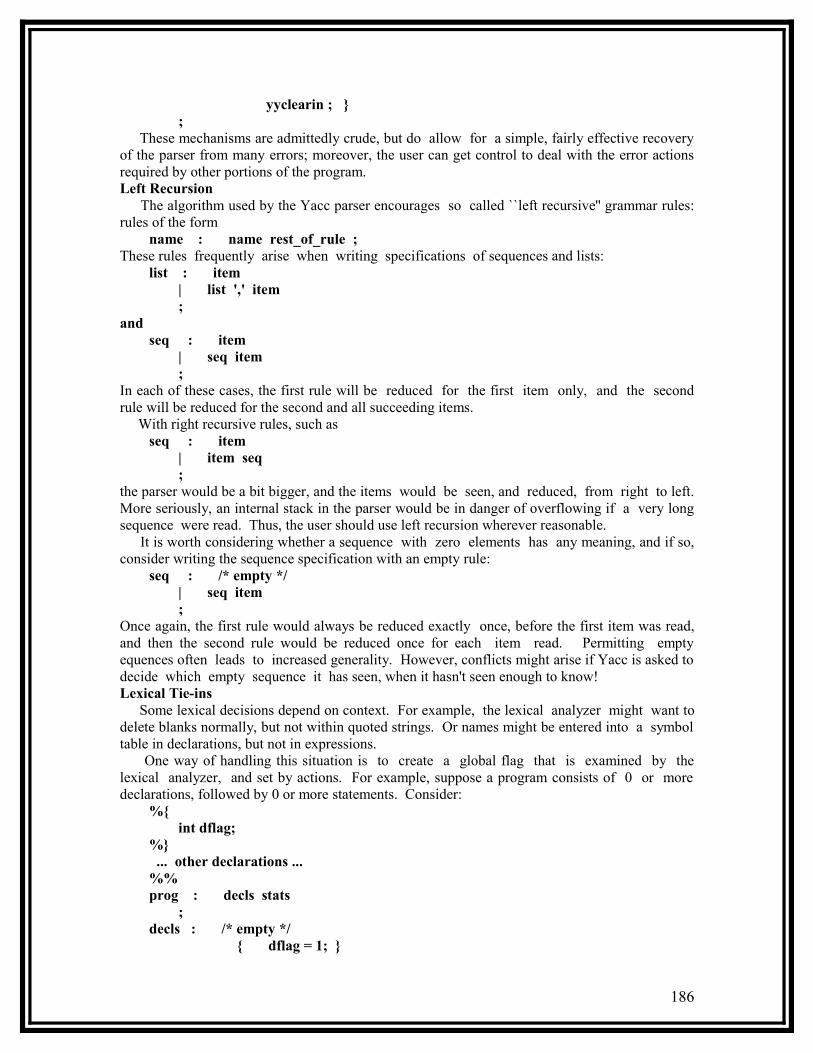
yyclearin ; } ; These mechanisms are admittedly crude, but do allow for a simple, fairly effective recovery of the parser from many errors; moreover, the user can get control to deal with the error actions required by other portions of the program.Left Recursion The algorithm used by the Yacc parser encourages so called ``left recursive'' grammar rules: rules of the form name : name rest_of_rule ;These rules frequently arise when writing specifications of sequences and lists: list : item | list ',' item ;and seq : item | seq item ;In each of these cases, the first rule will be reduced for the first item only, and the second rule will be reduced for the second and all succeeding items. With right recursive rules, such as seq : item | item seq ;the parser would be a bit bigger, and the items would be seen, and reduced, from right to left. More seriously, an internal stack in the parser would be in danger of overflowing if a very long sequence were read. Thus, the user should use left recursion wherever reasonable. It is worth considering whether a sequence with zero elements has any meaning, and if so, consider writing the sequence specification with an empty rule: seq : /* empty */ | seq item ;Once again, the first rule would always be reduced exactly once, before the first item was read, and then the second rule would be reduced once for each item read. Permitting empty equences often leads to increased generality. However, conflicts might arise if Yacc is asked to decide which empty sequence it has seen, when it hasn't seen enough to know!Lexical Tie-ins Some lexical decisions depend on context. For example, the lexical analyzer might want to delete blanks normally, but not within quoted strings. Or names might be entered into a symbol table in declarations, but not in expressions. One way of handling this situation is to create a global flag that is examined by the lexical analyzer, and set by actions. For example, suppose a program consists of 0 or more declarations, followed by 0 or more statements. Consider: %{ int dflag; %} ... other declarations ... %% prog : decls stats ; decls : /* empty */ { dflag = 1; }
186

| decls declaration ; stats : /* empty */ { dflag = 0; } | stats statement ; ... other rules ...The flag dflag is now 0 when reading statements, and 1 when reading declarations, except for the first token in the first statement. This token must be seen by the parser before it can tell that the declaration section has ended and the statements have begun. In many cases, this single token exception does not affect the lexical scan. This kind of ``backdoor'' approach can be elaborated to a noxious degree. Nevertheless, it represents a way of doing some things that are difficult, if not impossible, to do otherwise.Reserved Words Some programming languages permit the user to use words like ``if'', which are normally reserved, as label or variable names,provided that such use does not conflict with the legal use of these names in the programming language. This is extremely hard to do in the framework of Yacc; it is difficult to pass information to the lexical analyzer telling it ``this instance of `if' is a keyword, and that instance is a variable''. The user can make a stab at it, using the mechanism described in the last subsection, but it is difficult. A number of ways of making this easier are under advisement. Until then, it is better that the keywords be reserved; that is, be forbidden for use as variable names. There are powerful stylistic reasons for preferring this, anyway.
Example This example gives the complete Yacc specification for a small desk calculator; the desk calculator has 26 registers, labeled ``a'' through ``z'', and accepts arithmetic expressions made up of the operators +, -, *, /, % (mod operator), & (bitwise and), | (bitwise or), and assignment. If an expression at the top level is an assignment, the value is not printed; otherwise it is. As in C, an integer that begins with 0 (zero) is assumed to be octal; otherwise, it is assumed to be decimal. As an example of a Yacc specification, the desk calculator does a reasonable job of showing how precedence and ambiguities are used, and demonstrating simple error recovery. The major oversimplifications are that the lexical analysis phase is much simpler than for most applications, and the output is produced immediately, line by line. Note the way that decimal and octal integers are read in by the grammar rules; This job is probably better done by the lexical analyzer.
%{# include <stdio.h># include <ctype.h>int regs[26];int base;%}%start list%token DIGIT LETTER%left '|'%left '&'%left '+' '-'%left '*' '/' '%'%left UMINUS /* supplies precedence for unary minus */%% /* beginning of rules section */
187

list : /* empty */ | list stat '\n' | list error '\n' { yyerrok; } ;
stat : expr { printf( "%d\n", $1 ); } | LETTER '=' expr { regs[$1] = $3; } ;expr : '(' expr ')' { $$ = $2; } | expr '+' expr { $$ = $1 + $3; } | expr '-' expr { $$ = $1 - $3; } | expr '*' expr { $$ = $1 * $3; } | expr '/' expr { $$ = $1 / $3; } | expr '%' expr { $$ = $1 % $3; } | expr '&' expr { $$ = $1 & $3; } | expr '|' expr { $$ = $1 | $3; } | '-' expr %prec UMINUS { $$ = - $2; } | LETTER { $$ = regs[$1]; } | number ;
number : DIGIT { $$ = $1; base = ($1==0) ? 8 : 10; } | number DIGIT { $$ = base * $1 + $2; } ;
%% /* start of programs */
yylex() { /* lexical analysis routine */ /* returns LETTER for a lower case letter, yylval = 0 through 25 */ /* return DIGIT for a digit, yylval = 0 through 9 */ /* all other characters are returned immediately */
int c;
while( (c=getchar()) == ' ' ) {/* skip blanks */ }
188
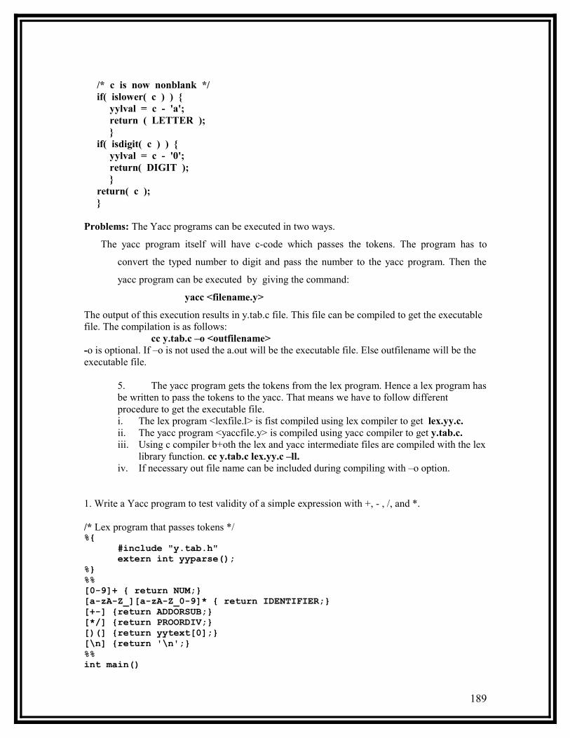
/* c is now nonblank */ if( islower( c ) ) { yylval = c - 'a'; return ( LETTER ); } if( isdigit( c ) ) { yylval = c - '0'; return( DIGIT ); } return( c ); }
Problems: The Yacc programs can be executed in two ways.
The yacc program itself will have c-code which passes the tokens. The program has to
convert the typed number to digit and pass the number to the yacc program. Then the
yacc program can be executed by giving the command:
yacc <filename.y>
The output of this execution results in y.tab.c file. This file can be compiled to get the executable file. The compilation is as follows:
cc y.tab.c –o <outfilename>-o is optional. If –o is not used the a.out will be the executable file. Else outfilename will be the executable file.
5. The yacc program gets the tokens from the lex program. Hence a lex program has be written to pass the tokens to the yacc. That means we have to follow different procedure to get the executable file.i. The lex program <lexfile.l> is fist compiled using lex compiler to get lex.yy.c.ii. The yacc program <yaccfile.y> is compiled using yacc compiler to get y.tab.c.iii. Using c compiler b+oth the lex and yacc intermediate files are compiled with the lex
library function. cc y.tab.c lex.yy.c –ll.iv. If necessary out file name can be included during compiling with –o option.
1. Write a Yacc program to test validity of a simple expression with +, - , /, and *.
/* Lex program that passes tokens */%{
#include "y.tab.h"extern int yyparse();
%}%%[0-9]+ { return NUM;}[a-zA-Z_][a-zA-Z_0-9]* { return IDENTIFIER;}[+-] {return ADDORSUB;}[*/] {return PROORDIV;}[)(] {return yytext[0];}[\n] {return '\n';}%% int main()
189
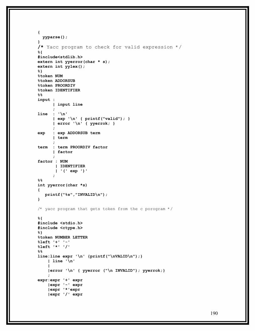
{ yyparse();}/* Yacc program to check for valid expression */%{#include<stdlib.h>extern int yyerror(char * s);extern int yylex();%}%token NUM%token ADDORSUB%token PROORDIV%token IDENTIFIER%%input : | input line
;line : '\n' | exp '\n' { printf("valid"); } | error '\n' { yyerrok; }
;exp : exp ADDORSUB term | term
;term : term PROORDIV factor | factor
;factor : NUM | IDENTIFIER | '(' exp ')'
;%%int yyerror(char *s){ printf("%s","INVALID\n");} /* yacc program that gets token from the c porogram */
%{#include <stdio.h>#include <ctype.h>%}%token NUMBER LETTER%left '+' '-'%left '*' '/'%%line:line expr '\n' {printf("\nVALID\n");} | line '\n' | |error '\n' { yyerror ("\n INVALID"); yyerrok;} ;expr:expr '+' expr |expr '-' expr |expr '*'expr |expr '/' expr
190

| NUMBER | LETTER ;%%main(){yyparse();}yylex(){char c;while((c=getchar())==' ');if(isdigit(c)) return NUMBER;if(isalpha(c)) return LETTER;return c;}yyerror(char *s){printf("%s",s);}
2. Write a Yacc program to recognize validity of a nested ‘IF’ control statement and display levels of nesting in the nested if.
/* Lex program to pass tokens */%{
#include “y.tab.h”%}digit [0-9]num {digit} + (“.” {digit}+)?binopr [+-/*%^=> <&|”= =”| “!=” | “>=” | “<=”unopr [~!]char [a-zA-Z_]id {char}({digit} | {char})*space [ \t]%% {space} ; {num} return num; { binopr } return binopr; { unopr } return unopr; { id} return id “if” return if . return yytext[0];%%NUMBER {DIGIT}+/* Yacc program to check for the valid expression */%{#include<stdio.h>int cnt;%}%token binopr
191

%token unop%token num%token id%token if%%foo: if_stat { printf(“valid: count = %d\n”, cnt); cnt = 0;
exit(0); }| error { printf(“Invalid \n”); }
if_stat: token_if ‘(‘ cond ‘)’ comp_stat {cnt++;}cond: expr
;expr: sim_exp
| ‘(‘ expr ‘)’| expr binop factor| unop factor;
factor: sim_exp| ‘(‘ expr ‘)’;
sim_exp: num| id;
sim_stat: expr ‘;’| if;
stat_list: sim_stat| stat_list sim_stat;
comp_stat: sim_stat| ‘{‘ stat_list ‘}’;
%%main(){
yyparse();}yyerror(char *s){
printf(“%s\n”, s);exit(0);
}
3. Write a Yacc program to recognize a valid arithmetic expression that uses +, - , / , *.
%{#include<stdio.h>#include <type.h>
%}
192

% token num% left '+' '-'% left '*' '/'%%st : st expn '\n' {printf ("valid \n"); }
| | st '\n'| error '\n' { yyerror ("Invalid \n"); };
%%void main()
{yyparse (); return 0 ;
}yylex(){
char c;while (c = getch () ) == ' ')
if (is digit (c))return num;return c;
}yyerror (char *s){
printf("%s", s);}
4. Write a yacc program to recognize an valid variable which starts with letter followed by a digit. The letter should be in lowercase only.
/* Lex program to send tokens to the yacc program */
%{#include "y.tab.h"
%}%%[0-9] return digit;[a-z] return letter;[\n] return yytext[0];. return 0;%%
/* Yacc program to validate the given variable */
%{#include<type.h>
193

%}% token digit letter;%%ident : expn '\n' { printf ("valid\n"); exit (0); }
;expn : letter
| expn letter| expn digit| error { yyerror ("invalid \n"); exit (0); };
%%main(){
yyparse();}yyerror (char *s){
printf("%s", s);}
/* Yacc program which has c program to pass tokens */
%{#include <stdio.h>#include <ctype.h>%}%token LETTER DIGIT%%st:st LETTER DIGIT '\n' {printf("\nVALID");} | st '\n' | | error '\n' {yyerror("\nINVALID");yyerrok;} ;%% main(){yyparse();}yylex(){char c;while((c=getchar())==' ');if(islower(c)) return LETTER;if(isdigit(c)) return DIGIT;return c;}yyerror(char *s) { printf("%s",s); }
194
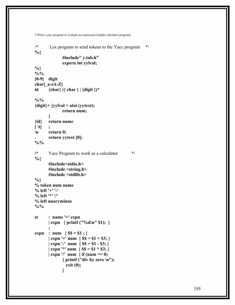
5.Write a yacc program to evaluate an expression (simple calculator program).
/* Lex program to send tokens to the Yacc program */%{
#include" y.tab.h"expern int yylval;
%}%%[0-9] digitchar[_a-zA-Z] id {char} ({ char } | {digit })*
%%{digit}+ {yylval = atoi (yytext);
return num;}
{id} return name[ \t] ;\n return 0;. return yytext [0];%%
/* Yacc Program to work as a calculator */%{
#include<stdio.h>#include <string.h>#include <stdlib.h>
%}% token num name% left '+' '-'% left '*' '/'% left unaryminus%%
st : name '=' expn| expn { printf ("%d\n" $1); };
expn : num { $$ = $1 ; }| expn '+' num { $$ = $1 + $3; }| expn '-' num { $$ = $1 - $3; }| expn '*' num { $$ = $1 * $3; }| expn '/' num { if (num == 0)
{ printf ("div by zero \n"); exit (0);}
195
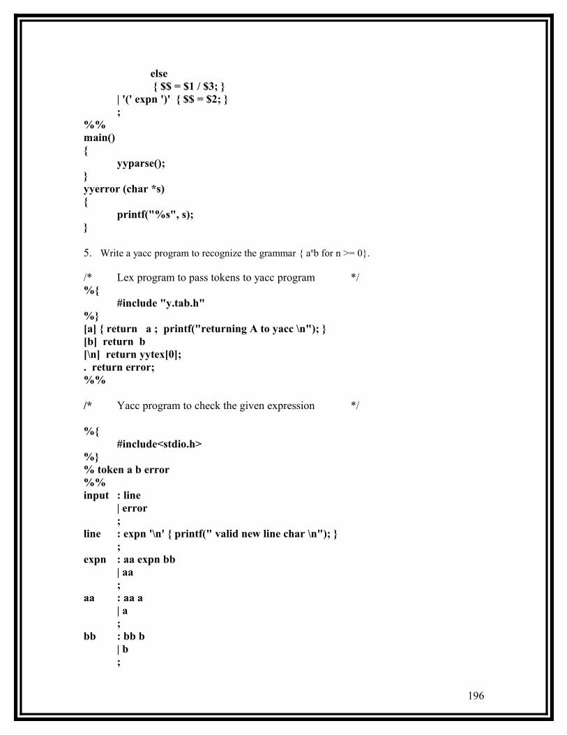
else { $$ = $1 / $3; }
| '(' expn ')' { $$ = $2; };
%% main(){
yyparse();}yyerror (char *s){
printf("%s", s);}
5. Write a yacc program to recognize the grammar { anb for n >= 0}.
/* Lex program to pass tokens to yacc program */%{
#include "y.tab.h"%}[a] { return a ; printf("returning A to yacc \n"); }[b] return b[\n] return yytex[0];. return error;%%
/* Yacc program to check the given expression */
%{#include<stdio.h>
%}% token a b error%%input : line
| error;
line : expn '\n' { printf(" valid new line char \n"); };
expn : aa expn bb| aa;
aa : aa a| a;
bb : bb b| b;
196

error : error { yyerror ( " " ) ; }
%% main(){
yyparse();}yyerror (char *s){
printf("%s", s);}
/* Yacc to evaluate the expression and has c program for tokens */
%{/* 6b.y {A^NB N >=0} */#include <stdio.h>%}%token A B%%st:st reca endb '\n' {printf("String belongs to grammar\n");} | st endb '\n' {printf("String belongs to grammar\n");} | st '\n' | error '\n' {yyerror ("\nDoes not belong to grammar\n");yyerrok;} | ;reca: reca enda | enda;enda:A;endb:B;%%main(){yyparse();}yylex(){char c;while((c=getchar())==' ');if(c=='a') return A;if(c=='b') return B;return c;}yyerror(char *s) {fprintf(stdout,"%s",s);}
7. Write a program to recognize the grammar { anbn | n >= 0 }
197
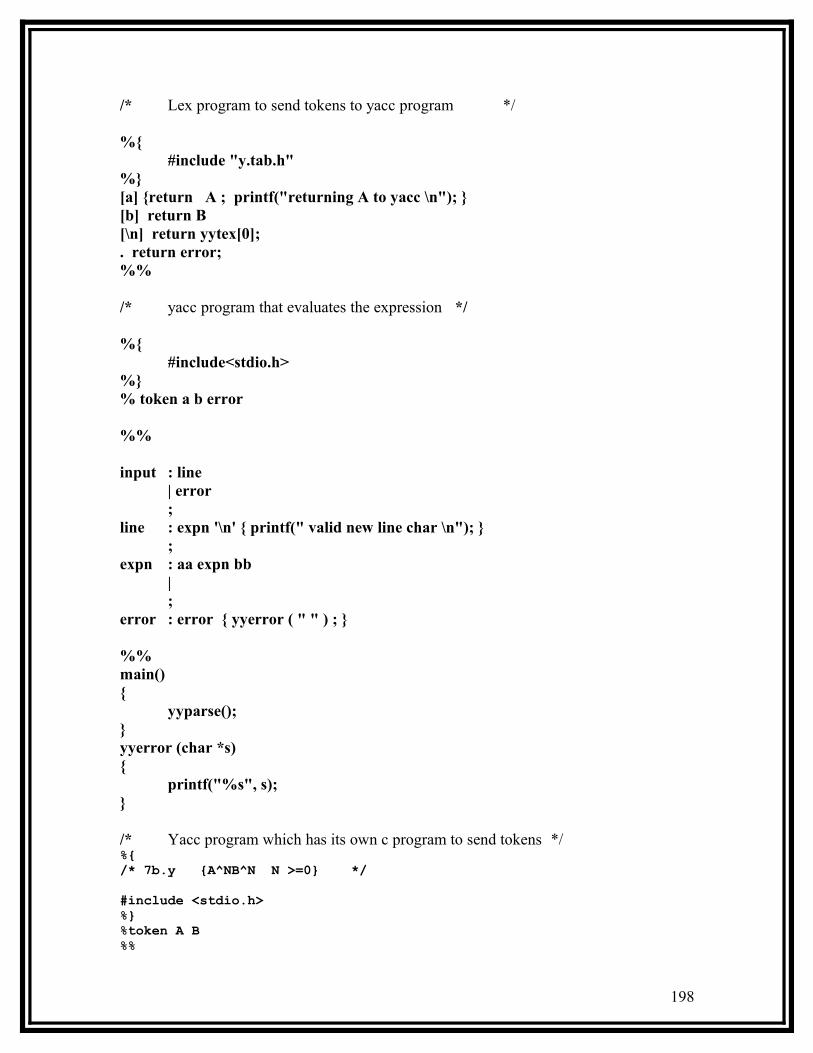
/* Lex program to send tokens to yacc program */
%{#include "y.tab.h"
%}[a] {return A ; printf("returning A to yacc \n"); }[b] return B[\n] return yytex[0];. return error;%%
/* yacc program that evaluates the expression */
%{#include<stdio.h>
%}% token a b error
%%
input : line| error;
line : expn '\n' { printf(" valid new line char \n"); };
expn : aa expn bb| ;
error : error { yyerror ( " " ) ; }
%% main(){
yyparse();}yyerror (char *s){
printf("%s", s);}
/* Yacc program which has its own c program to send tokens */%{/* 7b.y {A^NB^N N >=0} */#include <stdio.h>%}%token A B%%
198
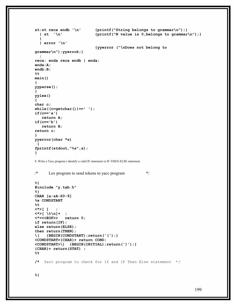
st:st reca endb '\n' {printf("String belongs to grammar\n");} | st '\n' {printf("N value is 0,belongs to grammar\n");} | | error '\n' {yyerror ("\nDoes not belong to grammar\n");yyerrok;} ;reca: enda reca endb | enda;enda:A;endb:B;%%main(){yyparse();}yylex(){char c;while((c=getchar())==' ');if(c=='a') return A;if(c=='b') return B;return c;}yyerror(char *s) {fprintf(stdout,"%s",s);}8. Write a Yacc program t identify a valid IF statement or IF-THEN-ELSE statement.
/* Lex program to send tokens to yacc program */
%{#include "y.tab.h"%}CHAR [a-zA-Z0-9]%x CONDSTART%%<*>[ ] ;<*>[ \t\n]+ ;<*><<EOF>> return 0;if return(IF);else return(ELSE);then return(THEN);\( {BEGIN(CONDSTART);return('(');}<CONDSTART>{CHAR}+ return COND;<CONDSTART>\) {BEGIN(INITIAL);return(')');}{CHAR}+ return(STAT) ;%%/* Yacc program to check for If and IF Then Else statement */
%{
199

#include<stdio.h>%}%token IF COND THEN STAT ELSE%%Stat:IF '(' COND ')' THEN STAT {printf("\n VALId Statement");} | IF '(' COND ')' THEN STAT ELSE STAT {printf("\n VALID Statement");} | ;%%main(){ printf("\n enter statement "); yyparse();}yyerror (char *s){ printf("%s",s);} /* Yacc program that has c program to send tokens */
%{#include <stdio.h>#include <ctype.h>
%}%token if simple% noassoc reduce% noassoc else%%start : start st ‘\n’
|;
st : simple| if_st;
if_st : if st %prec reduce { printf (“simple\n”); }| if st else st {printf (“if_else \n”); };
%%int yylex(){ int c;
c = getchar();switch ( c ){
case ‘i’ : return if;case ‘s’ : return simple;case ‘e’ : return else;default : return c;
}}main ()
200

{ yy parse(); }yyerror (char *s){
printf("%s", s);}
201