Chapter 6 EPOLLS Database of Lateral Spreads · EPOLLS Database of Lateral Spreads 6.1....

Chapter 6

EPOLLS Database of Lateral Spreads

6.1. Introduction.

As pointed out by Glaser (1993; 1994), assembling a database of field case studies is alaborious, yet critical, task in the development of an empirical model for lateral spreading. TheEPOLLS model was derived from the database described in this chapter and tabulated inAppendix A. Data were compiled on 78 lateral spreads from 16 earthquakes in western NorthAmerica and eastern Asia, mostly in California, Alaska, and Japan. These case studies aredescribed, in general terms, in the next section. Many of these lateral spreads are also in thedatabase compiled by Bartlett and Youd (1992b), although case studies from eight additionalearthquakes were included in the EPOLLS database. The site investigation reports and otherreference materials used in assembling the EPOLLS database are listed in Appendix B.

Only lateral spreads conforming to the definition adopted in Sections 3.1 and 5.1 werecompiled in the EPOLLS database. "Lateral spreads" more correctly associated with the slumpingof embankments or the outward rotation of retaining walls were not compiled in the EPOLLSdatabase. For example, port facilities constructed by loose filling behind quay walls are oftenheavily damaged by increased active earth pressures that result from liquefaction in the backfill.The resulting lateral movements in the zone immediately behind these walls do not constitute alateral spread suitable for the EPOLLS database. Moreover, sites subjected to lateral spreadingover a fairly large area, but with massive earth-retaining structures (concrete caissons, cellularcofferdams, rock-fill dikes) along the toe are not included in the EPOLLS database. On the otherhand, several sites in the EPOLLS database have relatively flexible sheet pile walls along the toeof the slide. In these cases, the flexible wall was judged to have a negligible effect on thedeformation of the comparably large sliding mass of the lateral spread. Statistical analyses duringdevelopment of the EPOLLS model confirmed this hypothesis by showing that the deformationof these sites were not substantially different than similar sites without a wall.

To be included in the EPOLLS database, a post-earthquake site investigation mustspecifically link lateral spreading to soil liquefaction in a subsurface deposit. Evidence forliquefaction includes surface manifestations such as sand boils or the analysis of in situpenetration tests that confirm liquefaction as the cause of the ground failure.

79

80Alan F. Rauch Chapter 6. EPOLLS Database of Lateral Spreads

Having selected the EPOLLS case studies, appropriate parameters were then chosen forcompilation in the database. These variables are grouped into four categories: (1) Seismological parameters include the earthquake magnitude and source distance, as well

as the intensity of shaking at the case study site. (2) Geometrical parameters indicate the area and shape of the surface of the lateral spread. (3) Topographical parameters include the surface slope and free face height. (4) Geotechnical parameters encompass all variables derived from soil borings such as the

thickness of liquefied soil, penetration resistance, and grain size characteristics.The parameters in each of these categories are discussed in Sections 6.3 through 6.7.

The variables chosen for the EPOLLS database reflect the physical mechanics ofliquefaction and lateral spreading discussed in Chapter 3. However, only parameters that can bedefined with reasonable accuracy and ease for a lateral spread in the field were chosen for theEPOLLS database. For example, it is recognized that the shear resistance of the liquefied soildeposit plays a role in controlling the magnitude of deformations in a lateral spread. However,the residual shear strength of a liquefied natural soil is difficult to determine from laboratory testsand is almost never known with confidence in the study of lateral spreads. Hence, in the EPOLLSdatabase, the shear strength of the liquefied soil is represented only indirectly with the in situpenetration resistance. No parameters from laboratory strength tests were compiled in theEPOLLS database.

The amount of information available varies considerably among the different EPOLLScase studies. At a minimum, measured displacements of the ground surface must be available fora lateral spread to be included in the database. Many of the EPOLLS case studies are thoroughlydocumented, while little quantitative data are available for other case studies. Since the geologicsource of nearly all large earthquakes in this century have been established, the seismologicalparameters are available for every EPOLLS case study. Information on the surface topographyis available for most of the case studies, while soil borings are available for only about threequarters of the EPOLLS database. However, many of the EPOLLS parameters could not bedefined for all case studies. These "missing values", which require special consideration duringmodel development, appear as blanks in the database tabulation in Appendix A.

6.2. Overview of Case Studies.

1906 San Francisco, California, EarthquakeFour case studies of lateral spreading resulting from this earthquake are included in the

EPOLLS database. Two of these case studies (Slide Nos. 1 and 2) are within the city of SanFrancisco, in formerly low-lying areas filled with loose soils during early development of the city.Slide No. 3 damaged a bridge across the Salinas River near Monterey Bay, while Slide No. 4damaged a bridge near the southern end of San Francisco Bay. Displacements at these sites were


determined mostly from contemporary reports of earthquake damage. Slide No. 2 is shown inFigure 6.1.

1923 Kanto, Japan, EarthquakeThis infamous earthquake caused tremendous destruction and loss of life in the Tokyo

area. Lateral spreading occurred along the Furu-Tone River in the city of Kasukabe, north ofTokyo. Displacements for one EPOLLS case study were measured by the lateral offset of a citystreet.

1948 Fukui, Japan, EarthquakeFour EPOLLS case studies were compiled from investigations of liquefaction damage in

this earthquake. These lateral spreads occurred on both sides of the Yoshino River, a tributaryof the Kuzuryu River, near the west coast of the island of Honshu. Surface displacements weremeasured from aerial photographs of the area, taken before and after the earthquake. Two casestudies (Slide Nos. 8 and 9) are depicted in Figure 6.2.

1964 Prince William Sound, Alaska, EarthquakeThis extremely large-magnitude earthquake caused extensive damage across southern

Alaska. Fifteen lateral spread case studies were compiled for the EPOLLS database. In each case,displacements were determined from the offset of bridge piers along the Alaska Railroad, theSeward-Anchorage Highway, and the Glenn Highway. In some of these cases, displacements wereestimated many years later by measuring how far the rail bearing plates were moved duringrepairs after the earthquake. Good maps showing cracks in the ground surface, useful indelineating the area and direction of sliding, are available for many of these sites. An exampleof these maps is shown in Figure 6.3. Here, three lateral spreads (Slide Nos. 10 through 12)damaged railroad and highway bridges crossing the Resurrection River.

1964 Niigata, Japan, EarthquakeExtensive liquefaction-induced ground failures occurred throughout the west-coast city of

Niigata. Fourteen lateral spreads were identified for the EPOLLS database: eleven of these slideswere in Niigata along the banks of the Shinano River, one was on the west bank of the AganoRiver, and two cases were along the much smaller Tsusen River. Slide Nos. 31 and 32, locatedjust east of the Shinano River, are shown in Figure 6.4 and Slide Nos. 37 and 38, along theTsusen River, are shown in Figure 6.5. In all fourteen case studies, displacements of the groundsurface were measured from aerial photographs taken before and after the earthquake. The lateralspreads in Niigata, which are some of the best-documented case studies in the EPOLLS database,involved very large surface displacements.

1971 San Fernando, California, EarthquakeTwo lateral spreads were identified in San Fernando, California, which is at the north end

of the Los Angeles metropolitan area. Slide No. 40 involved the lateral deformation of a fill


underlying the Joseph Jensen Water Filtration Plant. Deformations in this area were determinedfrom both aerial photographs and optical surveys, with adjustments for tectonic movements inthe area. Slide No. 41, shown in Figure 6.6, extends from the San Fernando Valley Juvenile Hallfacility to the Upper Van Norman Reservoir. Here, displacements were measured from aerialphotographs, optical surveys, and the offsets of streets.

1976 Guatemala EarthquakeEPOLLS Slide No. 42 occurred in the Villalobos River Delta on the shore of Lake

Amatitlan in Guatemala. Maximum displacements were estimated from the cumulative offsetsmeasured across fissures in the ground surface.

1979 Imperial Valley, California, EarthquakeOccurring south of the Salton Sea in the Imperial Valley of southern California, two

lateral spreads were included in the EPOLLS database. Slide No. 43 is a well-documented lateralspread of fairly small area in which displacements were determined mostly from the offset of asmall irrigation canal. Very small displacements, indicative of the reported surface cracking inthe area, were assumed for Slide No. 44. 1983 Nihonkai-Chubu, Japan, Earthquake

Five well-documented case studies were obtained with surface displacements determinedfrom the analysis of aerial photographs. These lateral spreads all occurred in the west coast cityof Noshiro, Japan. Slide Nos. 45 through 48 are shown in Figure 6.7. The surface deformationin Slide No. 49, with 187 measured displacement vectors, is the most extensively documentedin the EPOLLS database.

1983 Borah Peak, Idaho, EarthquakeTwo lateral spreads underlain by gravelly soils were studied following this earthquake in

south-central Idaho. Because of the high gravel content in the liquefiable soils at both sites,Standard Penetration Tests (SPTs) are unreliable. Hence, the geotechnical EPOLLS parametersfor these sites were derived from Becker Penetration Test logs that were converted to equivalentSPT blowcounts (see Section 7.2). Since the high gravel content in the underlying soil might havea significant impact on lateral spreading, these two case studies were investigated as possibleoutliers during development of the EPOLLS model. However, statistical analysis indicated thatthe deformation of these two sites was not outside the trend of the other case studies in thedatabase.

1987 Superstition Hills, California, EarthquakeOnly one case study was recorded from this earthquake. The lateral spread developed at

the Wildlife Liquefaction Array located along the Alamo River, southeast of the Salton Sea insouthern California. This site has been instrumented by the U.S. Geological Survey to record theonset of soil liquefaction during an earthquake.


1989 Loma Prieta, California, EarthquakeFrom ground failures caused by this earthquake, five case studies were compiled. This

earthquake caused extensive damage in the San Francisco metropolitan area. In two areas in thecity of San Francisco, where lateral spreading occurred in the 1906 earthquake, evidence of soilliquefaction was observed again in 1989. However, no consistent pattern of horizontal movementwas observed in 1989. Thus, these two sites were included in the EPOLLS database with a zeroaverage horizontal displacement. Another EPOLLS case study (Slide No. 55) was a lateral spreadthat developed at Moss Landing Spit on the eastern shore of Monterey Bay. Two other EPOLLScase studies, Slide Nos. 56 and 57, are lateral spreads that developed in the agricultural fieldsalong the Pajaro River just east of Watsonville, California.

1990 Luzon, Philippines, EarthquakeFour lateral spreads, occurring along the Pantal River in the city of Dagupan, Philippines,

were included in the database. Dagupan is located north of Manila on the west coast of the islandof Luzon. Displacements at these four sites were estimated from damage to structures in the area.

1991 Telire-Limon, Costa Rica, EarthquakeDamages to one highway bridge and four railroad bridges were used to estimate

displacements for five case studies from this earthquake. Only minimal information is availablefrom these sites.

1993 Hokkaido Nansei-oki, Japan, EarthquakeIn the floodplain of the Shiribeshi-toshibetsu River, near the southwest coast of the island

of Hokkaido, nine lateral spreads were documented. Displacements, surface cracks, and sand boilswere mapped from aerial photographs of the area. Slide Nos. 115 through 117 are shown inFigure 6.8.

1994 Northridge, California, EarthquakeThis earthquake caused damages over roughly the same area as the 1971 San Fernando

earthquake. At the San Fernando Valley Juvenile Hall site (Slide No. 118), much smallerdisplacements were reported in 1994 than for the same site in 1971. The other case studiesobtained from this earthquake were not extensively documented.

1995 Hyogoken-Nanbu, Japan, EarthquakeThis earthquake caused massive liquefaction damage in the port city of Kobe, Japan,

located on the western side of Osaka Bay. However, no case studies of lateral spreading havebeen reported that would be suitable for inclusion in the EPOLLS database. Most of theliquefaction damage in Kobe occurred along the waterfront and on man-made islands in the city.These areas were typically constructed by filling behind large, sand-filled, concrete caissonstructures. While extensive lateral deformation of the ground in Kobe resulted from soilliquefaction, none of these failures appear to have occurred in the absence of a massive earth-


retaining structure. Therefore, no case studies from this earthquake are in the EPOLLS database.

6.3. Horizontal and Vertical Displacements.

The average, standard deviation, and maximum measured horizontal and verticaldisplacements are compiled in the EPOLLS database. These six values for the surfacedeformation in a lateral spread are identified with: • Avg_Horz is the average horizontal displacement, • StD_Horz is the standard deviation of the horizontal displacements, • Max_Horz is the maximum observed horizontal displacement, • Avg_Vert is the average vertical displacement, • StD_Vert is the standard deviation of the vertical displacements, • Max_Vert is the maximum observed vertical displacement.Settlements are recorded as positive vertical displacements, while uplift or heaving is taken asa negative vertical displacement.

The above values were computed using all of the measured displacement magnitudesavailable in the published site investigation reports. The numbers of horizontal and verticaldisplacement vectors measured on each lateral spread are listed in the EPOLLS database.However, in about one-third of the case studies, few displacement magnitudes were measured.In these cases, the average or maximum displacement was approximated from whateverinformation was available. For example, in a post-earthquake damage report, the average ormaximum movement might have been approximated by an observer at the site. In some cases,the compression of a bridge was used to estimate the average deformation, with one half of themovement attributed to lateral spreads on each side of the stream.

When horizontal and vertical displacements were directly measured in the investigationsof the EPOLLS case studies, movements were determined in one of four ways: (1) Offsets in streets, curbs, sidewalks, fences, lined drainage channels, etc. that cross a lateral

spread, as well as the compression or extension of bridges and pipelines. (2) Cumulative offsets across fissures in the ground surface, measured along traverse lines. (3) Optical surveys used to locate reference points, with displacements determined by

comparing positions before and after an earthquake. (4) Analysis of aerial photographs, taken before and after an earthquake, showing the

movement of selected reference points.For the optical surveys and aerial photographic analysis, reference points included utility poles,fence posts, manhole covers, corners of drainage channels, corners on small buildings, and othersimilar points.

Reference points for measuring displacements are assumed to have moved with the


surrounding ground without imparting a significant restraint to the local deformation. While thismay not be true in the strictest sense, the reported measurements are believed to give areasonable indication of the free-field, horizontal, surface deformations. However, because ofpossible loss of bearing capacity, some reference points may have settled more than thesurrounding ground surface. Other reference structures may have been subjected to tilting, or evenupward floating, which would also affect the measured vertical displacement. In general, thereported vertical displacements are considered to be less reliable than the horizontal displacementsas measures of the free-field deformation on a lateral spread.

Regardless of the method used to determine surface displacements, some error isassociated with these measurements. However, it is reasonable to assume that these errors arerandom. Moreover, while the displacement at any given point may not be measured with greataccuracy, the average displacement computed from measurements at multiple locations shouldbe closer to the true average displacement of a lateral spread. Consequently, the average andstandard deviation of the surface displacements are known with greater confidence than thedisplacement at any single location. As more displacement vectors are measured, the average andstandard deviation are known with greater accuracy because these values are less sensitive torandom errors in the individual measurements. On the other hand, the maximum measureddisplacement is a single value known with much less confidence. In addition to possiblemeasurement error, the largest observed displacement might be significantly less than the truemaximum deformation, which might have occurred in an area where displacements were notdetermined.

In the EPOLLS case studies, displacements at specific locations are measured with thegreatest precision when lateral offsets in streets, etc. are measured. The magnitude of thesedisplacements are probably accurate to within a few centimeters. On the other hand, the precisionof the individual displacement magnitudes determined from aerial photographs is considerablyless. For example, the horizontal displacements measured in Niigata and Noshiro, Japan, arebelieved to be accurate to within only ± 72 cm and ± 13 cm, respectively. However, the analysisof aerial photographs usually yields many more measured displacement vectors across the surfacearea of the lateral spread. For this reason, the values of average, maximum, and standarddeviation of the displacements are often known with greater confidence when determined fromaerial photographs. Overall, it is difficult to quantitatively express the accuracy associated withthe displacements compiled in the EPOLLS database.

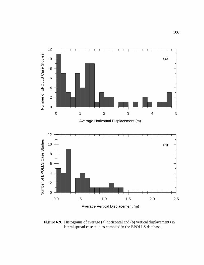
Histograms of the average displacements compiled in the EPOLLS database are shownin Figure 6.9. These plots give a picture of the dispersion of horizontal and vertical displacementmagnitudes in the database. As can be seen in Figure 6.9a, the average horizontal displacementis less than 1.6 m in most of the EPOLLS case studies. On the other hand, nine lateral spreadshad average horizontal displacements exceeding 3.0 m; all of these case studies occurred in 1964in Niigata, Japan. While the Niigata case studies involved very large displacements, most of the


EPOLLS case studies experienced small to moderate horizontal displacements. In addition, theaverage settlement in most of the EPOLLS case studies is less than 0.7 m, as indicated by thehistogram in Figure 6.9b. Hence, these histograms suggest that smaller and less damaging lateralspreads are probably not severely under-represented in the assembled database.

6.4. Seismological Parameters.

The EPOLLS seismological parameters represent the size and distance to the seismicsource, as well as the intensity of shaking at the site of the lateral spread. The seismologicalparameters are defined here and listed in Table A.2 of Appendix A.

Parameter: EQ_Mw = moment magnitude of the earthquake.Because it gives a more reliable measure of earthquake size, the moment magnitude scale

is preferred by many seismologists (Bolt 1993). As defined by Kanamori (1978), the momentmagnitude (Mw) is computed with:

The seismic moment (Mo, in dyne-cm = 10-7 N-m) is a measure of the work done by the fault

(6.1)

rupture. As explained in Chapter 7, the moment magnitude is used in the evaluation ofliquefaction resistance.

Parameter: EQ_Ms = surface-wave magnitude of the earthquake.The surface-wave magnitude (Ms) is an empirical measure commonly used to describe the

size of shallow, strong earthquakes. This magnitude scale is based on the largest measuredamplitude of the surface wave with a period of about 20 seconds (Bolt 1993).

Parameter: Focal_Depth = focal depth of the earthquake (kilometers).The focal depth is the depth of the earthquake hypocenter below the surface of the earth,

as illustrated in Figure 6.10.

Parameter: Epict_Dist = epicentral distance to the earthquake (kilometers).The epicentral distance is measured along the earth's surface from the lateral spread to the

epicenter of the earthquake (surface projection of the hypocenter), as illustrated in Figure 6.10.

Parameter: Hypoc_Dist = hypocentral distance to the earthquake (kilometers).The hypocentral distance is the shortest distance from the lateral spread to the earthquake

hypocenter (location where the fault rupture commences) as shown in Figure 6.10. For sitessubject to soil liquefaction, the epicentral distance is small enough to neglect the earth's


curvature. The hypocentral distance can then be computed from the focal depth and epicentraldistance with:

(6.2)

Parameter: Fault_Dist = shortest horizontal distance to the fault rupture (kilometers).The fault distance, also illustrated in Figure 6.10, is the shortest horizontal distance

(measured along the earth's surface) from the lateral spread to the surface projection of the faultrupture, or zone of seismic energy release, causing the earthquake. If the site falls within thesurface projection of the fault rupture, then the fault distance is zero. If the fault plane rupturesthe surface of the earth, then the fault distance is measured to the nearest surface rupture.

Parameter: Accel_max = peak horizontal acceleration at the ground surface (g's).This is the maximum horizontal acceleration that would occur at the surface of a site in

the absence of excess pore pressures or liquefaction generated by the earthquake. Ideally,Accel_max would be taken from ground motions recorded at a location next to a lateral spread;however, such recordings are rarely available in the immediate vicinity of an EPOLLS case study.For some sites in the EPOLLS database, the peak acceleration was estimated from peak valuesrecorded at stations in the area, with adjustments for distance to the earthquake source. For manyEPOLLS sites, the peak acceleration was estimated by earlier investigators and included in theirpublished site reports. The available data and published estimates of peak acceleration were alsosupplemented with predictions from empirical attenuation relationships. All of this informationwas considered in choosing an appropriate value of Accel_max for the EPOLLS case study sites.

Numerous empirical equations have been developed by seismologists over the years, withfrequent updates as additional data are collected from recent earthquakes. Estimates from severalof these equations were considered in assembling the EPOLLS database, but the values ofAccel_max compiled generally reflect estimates from two selected empirical attenuation equations.Both equations represent the geometric mean of the orthogonal horizontal acceleration recordsat a site. For earthquakes in western North America, an equation given by Boore et al. (1993)was primarily used. This equation was developed for "Class C" sites (sites with soils in the upper30 m having shear wave velocities between 180 and 360 m/s), typical of sites subject toliquefaction and lateral spreading. Using the variables defined above, the equation by Boore etal. (1993) can be written as:

However, Equation 6.3 is specifically valid only for earthquakes in western North America. An

(6.3)

attenuation equation for Japan, developed by Fukushima and Tanaka (1990), was primarily used


to estimate peak accelerations from earthquakes in the western Pacific. Again using thepreviously-defined EPOLLS variables, the equation given by Fukushima and Tanaka (1990) canbe written as:

where R is defined as the shortest distance to the fault rupture. However, for most of the Japanese

(6.4)

data used by Fukushima and Tanaka, the fault rupture was difficult to define and the hypocentraldistance was used for R. Hence, in compiling Accel_max for the EPOLLS case studies in easternAsia, Equation 6.4 was used with R = Hypoc_Dist.

Parameter: Duration = duration of strong earthquake motions (seconds).Here, a "bracketed duration" (Kramer 1996) is used to indicate the length of time the site

is subjected to strong ground motions during the earthquake. The duration is measured as the timebetween the first and last occurrence of a surface acceleration exceeding 0.05 g. When available,strong motion records from stations near the site of an EPOLLS case study were used to estimatethe duration of shaking. When no suitable records were available, an empirical correlationproposed by Krinitzsky et al. (1988) for sites with soft soils was used: • for plate margin earthquakes with Focal_Depth ≤ 19 km,

• for subduction zone earthquakes with Focal_Depth ≥ 20 km,

(6.5)

(6.6)

6.5. Geometrical Parameters.

In this section, the EPOLLS parameters that describe the geometry and dimensions of alateral spread are defined. A list of the database variables in this category is also given in TableA.3.

Parameter: Banded_Area? = TRUE for lateral spreads of the banded-area type, FALSE if thesurface area of the lateral spread is bounded on all sides.

This classification refers to the shape of the slide mass in plan. For lateral spreads withBanded_Area? = FALSE, a bounding line can be drawn that completely encloses the slide mass.Examples include Slide No. 9 in Figure 6.2, Slide Nos. 11 and 12 in Figure 6.3, and all of theslides in Figures 6.7 and 6.8. On the other hand, lateral spreads often occur in bands running


parallel to a stream or free face. In these "banded-area" cases (Banded_Area? = TRUE),horizontal displacements tend to be perpendicular to the stream and form surface fissures that areroughly parallel to the stream. While it is fairly easy to define the head and toe in lateral spreadsof this type, the flanks of the slide are generally undefined. Examples of banded-area lateralspreads include Slide Nos. 8 and 10 in Figures 6.2 and 6.3.

Parameter: Slide_Area = surface area of the slide mass (square meters).The slide area is the horizontal surface area of the lateral spread measured in plan view.

The slide area is undefined for banded-area type lateral spreads. When both sides of a stream aresubjected to extensive liquefaction and lateral spreading, the slide areas meet in the center of thestream as for the EPOLLS case studies shown in Figure 6.3.

Parameter: Slide_Length = length of slide area from head to toe (meters).The slide length, as indicated in Figure 5.1, is the horizontal distance from the head of

a lateral spread to the toe, measured in the prevailing direction of movement. When extensive soilliquefaction causes a lateral spread in the floodplain of a stream, the slide length is assumed toextend to the center of the stream.

Parameter: Divergence = divergence factor.The divergence factor represents the change in width of the slide mass as one moves from

the head toward the toe. A positive divergence factor indicates that the slide mass gets widertoward the toe, while a negative divergence factor indicates a narrowing of the slide area.Definition of the divergence factor is detailed in Figure 6.11. The divergence parameter wasdefined based on the hypothesis that displacements might be restrained by constriction of theflanks toward the toe, or deformations might increase if the flanks get progressively further apart.

6.6. Topographical Parameters.

This category of EPOLLS parameters includes variables representing the topography ofa lateral spread, such as surface slope. These variables are listed in Table A.4 of Appendix A.

Parameter: Direct_Slide = direction of sliding (degrees).The direction of sliding is measured as the angle in the horizontal plane between the

prevailing direction of movement and the maximum slope. The line of maximum slope is drawnperpendicular to a free face or the principle topographical contour lines. In most lateral spreads,Direct_Slide is zero. In some case studies, Direct_Slide is greater than zero becausedisplacements, such as the compression of a bridge, were measured in a direction that was notcoincident with the maximum slope direction.


Parameter: Free_Face? = TRUE if free face along toe, FALSE if no free face.A free face is any relatively abrupt, essentially vertical change in the topography along

the toe of the slide. A free face in a lateral spread is most commonly a stream bank but can alsobe a road cut, drainage channel, etc.

Parameter: Bulkhead? = TRUE if flexible wall along free face, FALSE if no wall or free face.Along a waterfront, it is not uncommon for a free face to be stabilized with an earth-

retaining wall. If this wall is massive, such as the large caisson structures used in building theport facilities in Kobe, Japan, an associated liquefaction failure does not conform to the definitionof a lateral spread and is not included in the EPOLLS database. However, if the wall is "flexible"(such as a steel sheet pile wall) and judged to not provide significant restraint to a large lateralspread behind the wall, the site can be used as an EPOLLS case study. The Bulkhead? categoryparameter is used to identify the EPOLLS cases studies where some type of flexible wall formsthe free face but is judged to provide minimal support to a relatively large lateral spread behindthe wall.

Parameter: Face_Height = height of free face, measured vertically from toe to crest (meters).The face height is measured vertically from the toe to the crest of the free face, as shown

in Figure 6.12. When the free face is a stream bank, the face height is measured from thesubmerged toe at the bottom of the stream. The height of a narrow levee at the top of a streambank is not included in the face height. If there is no free face, Face_Height equals zero.

Parameter: Top_%Slope = average slope across the surface of the lateral spread (percent).The surface slope is measured as the change in elevation over the horizontal distance from

the head to the toe of the lateral spread, as indicated in Figure 6.12. When a free face is present,the top slope is measured from the head of the slide to the crest of the free face. Narrow leveesat the tops of stream banks are ignored. Negative values of Top_%Slope indicate that the surfaceis inclined away from the direction of movement. A small negative surface slope is often foundin the flood plain of a stream with a lateral spread moving toward the free face of the streambank.

Parameter: Eff_%Slope = effective surface slope of the lateral spread (percent).The effective slope is defined as the change in elevation over horizontal distance from the

head of the slide to the toe of a free face, if present. This can be written in equation form as:

The effective surface slope combines the effects of face height and top surface slope into a single

(6.7)

variable. In an idealized sense, the effective slope represents the static stress driving the lateralspread.


Parameter: Bot_%Slope = average slope along the bottom of the liquefied deposit (percent).The bottom slope is measured as the change in elevation over the horizontal distance

along the bottom of the liquefied soil deposit underlying a lateral spread, as illustrated in Figure6.12. Like the top slope, a negative bottom slope indicates a slope in a direction opposite to theprevailing direction of movement. While this variable is classified as a topographical parameterin EPOLLS, evaluation of the subsurface soil conditions is required to define Bot_%Slope.

6.7. Geotechnical Parameters.

The geotechnical parameters in the EPOLLS database represent the soil conditionsunderlying a lateral spread. Based on an analysis of available geotechnical soil borings, theEPOLLS geotechnical parameters indicate the: • thickness of liquefied soil, • average shear resistance of the liquefied soil, • minimum shear resistance in the liquefied soil, • gradation of the liquefied soil, and • strength and permeability of unliquefied soil above and below the liquefied soil.Thirty-eight geotechnical parameters, discussed in this section and listed in Table A.5, weredefined for the EPOLLS database. To compile these parameters for 59 EPOLLS case studies, 248soil borings were analyzed. A computer program was written to process this data and computethe EPOLLS geotechnical parameters. Called "EPOLIQAN", for EPOLLS LIQuefaction ANalysis,this computer code is documented in Appendix C.

The EPOLLS geotechnical parameters are computed from the logs of soil borings withStandard Penetration Tests (SPTs). First, the measured SPT blowcounts (blows per foot) areconverted to a normalized, corrected value labeled as (N1)60. Based on the (N1)60 value, theliquefaction resistance of the soil is calculated along with the cyclic stress induced by theearthquake at the same depth. The factor of safety against liquefaction (FSliq) is then computedfor every SPT depth in the boring. A FSliq ≤ 1.0 is interpreted to mean the soil liquefied at thatdepth during the earthquake. The vertical profile of FSliq thus indicates the liquefied soil thicknessat each boring location. The empirical procedure used to analyze the soil boring data andcompute the factor of safety profile is discussed fully in Chapter 7. The geotechnical parametersdiscussed here are all based on values of (N1)60, factor of safety against liquefaction, and theliquefied thickness in the soil borings at the EPOLLS case study sites.

When Standard Penetration Tests are performed in a soil boring, the tests are typicallyconducted at depth intervals of one to two meters. The (N1)60 value and factor of safety againstliquefaction can be computed only at these discrete testing depths in the boring log. In addition,because the grain size distribution is usually determined from laboratory analysis of the SPTsamples, the soil gradation is often available only for these testing depths. Consequently, all of


the EPOLLS geotechnical parameters are computed directly or indirectly from data at the SPTlocations. For some parameters, an average value is calculated from data at all SPT locations inthe liquefied thickness. For example, the parameter FS_Min is the single minimum factor ofsafety determined at the depth of an SPT. On the other hand, the parameter FS_Liq is the averagefactor of safety in the liquefied thickness; that is, the factor of safety determined from each SPTin the liquefied thickness is averaged to give FS_Liq. Similarly, the parameter Fine_Liq is anaverage of the fines content measured at all depths in the liquefied thickness.

The depth to the top and bottom, as well as the thickness, of liquefied soil are alsocomputed from the SPT values in the soil boring logs. However, the boundaries between liquefiedand unliquefied soil usually fall between SPT depths. Thus, to estimate the liquefied thicknessin a boring log, a continuous, interpolated profile is needed. The procedure used to compute theinterpolated profile (to 0.1 m depth increments) in the EPOLIQAN program is discussed inSection 7.5. In some cases, however, the computed, interpolated profile is not a goodrepresentation of the field conditions. For example, the EPOLIQAN code may indicate anunliquefied sand seam in the middle of a much thicker liquefied deposit. While this is possible,it is usually reasonable to assume such a seam will liquefy due to pore pressure migration. Hence,to allow for interpretations based on engineering judgment, the liquefied thickness can bespecified by the user of the EPOLIQAN code (see Appendix C).

A summary of these considerations in the calculation of the EPOLLS geotechnicalparameters is presented in Table 6.1. In the middle two columns, calculation of the parametersusing only data from the SPT depths or the interpolated continuous soil profile is indicated. Someof the EPOLLS parameters are values from the SPT depths averaged over the liquefied thickness,which is either predicted from the interpolated profile or specified. In the EPOLIQAN code, theseparameters are actually computed twice: once using the predicted liquefied thickness, and asecond time using the specified liquefied thickness. The EPOLLS parameters that depend on theliquefied thickness are indicated by the entry in the last column of Table 6.1.

In addition, while a soil boring measures the soil conditions at one specific location, thegeotechnical parameters in the EPOLLS database must represent the subsurface conditions acrossthe entire area of a lateral spread. To represent the soil conditions across a lateral spread, datafrom all of the available soil borings are used to define the appropriate EPOLLS parameters.Hence, in the EPOLLS database, two values of each geotechnical parameter are listed: an Avg-parameter representing the average value across the site, and a Rng- parameter representing therange (maximum minus minimum values) across the site. For example, the parameter Avg-Z_GrWater represents the average depth to ground water, while Rng-Z_GrWater is the differencebetween the maximum and minimum depth to ground water across the site. Whether data isavailable from one or multiple soil borings, the Avg- and Rng- values are estimated from allavailable information. In particular, the Avg- and Rng- values of the liquefied thickness are bestestimated from the general engineering knowledge of the subsurface geology at the site. In


compiling the EPOLLS database, all available subsurface information was used, including datafrom in situ penetration tests other than SPT's. While the definition of Avg- and Rng- parametersis fairly subjective, this approach allows the engineer to use all available data to describe thesubsurface soil conditions.

Nineteen EPOLLS geotechnical parameters are defined in the list that follows. For each,an Avg- and Rng- value is compiled in the database for a maximum of 38 entries describing thesoil conditions beneath a lateral spread.

Parameter: Z_GrWater = depth to ground water (meters).This is the depth to the static ground water table, measured vertically from the surface.

Parameter: Z_TopLiq = depth to top of liquefied soil (meters).This depth is measured from the surface to the top of the shallowest liquefied soil

sublayer. Z_TopLiq is equal to the thickness of the unliquefied soil above the liquefied zone. Formany lateral spreads, the top of the liquefied soil coincides with the ground water table.

Parameter: Z_BotLiq = depth to bottom of liquefied soil (meters).This depth is measured to the bottom of the deepest liquefied soil sublayer. In

EPOLIQAN, the predicted value of Z_BotLiq does not exceed the maximum depth in a soilboring. When liquefaction is predicted at the very bottom of a soil boring, data from deeperpenetration tests are needed to establish the correct value of Z_BotLiq.

Parameter: Thick_Liq = thickness of liquefied soil (meters).The vertical thickness of liquefied soil can be defined in one of two general ways, as

depicted in Figure 6.13. The liquefied thickness (Thick_Liq) can be defined as the gross liquefiedthickness (equal to Z_BotLiq minus Z_TopLiq) or as the summation of the liquefied sublayerthicknesses. When only one soil layer liquefies, both definitions yield the same value ofThick_Liq. However, when more than one liquefied layer is expected, these two definitions cangive significantly different values. The choice between the two definitions for Thick_Liq issubjective and left to the judgment of the engineer. This choice should be made so that Thick_Liqbest represents the thickness of soil experiencing significant loss of shear strength in a lateralspread. The following guidelines are suggested: • If a major soil unit liquefies, with the possibility of thin, unliquefied seams, use the gross

liquefied thickness for Thick_Liq. • If liquefaction occurs in thin sublayers of the soil profile, use the summation of the

liquefied thicknesses for Thick_Liq. This distinction is further illustrated in Figure 6.13. For most of the EPOLLS cases studies,liquefaction occurred throughout most of a major soil unit and the gross liquefied thickness wasused.


Parameter: Index_Liq = index of liquefied thickness in the upper 20 meters.This parameter represents the net shear resistance of the soil profile, with more weight

given to the soil strength at shallower depths. The Index_Liq is based on a weighted indexproposed by Hamada et al. (1986) and computed over the upper 20 m of the soil profile.However, the index given by Hamada and his colleagues is not consistently defined for a soilboring that does not extend to a depth of 20 m. With this in mind, the weighted index proposedby Hamada et al. (1986) was normalized for the maximum depth of the soil boring to give theEPOLLS parameter Index_Liq:

Here, z is the depth in meters, zbot is the maximum depth (not exceeding 20 m) where FSliq is

(6.8)

determined, and ∆z is the depth increment to which FSliq is interpolated (∆z = 0.1 m in theEPOLIQAN code). At depths where liquefaction is predicted (FSliq≤1.0), the strength function isF = 1.0 - FSliq. At depths where FSliq>1.0 or in soils otherwise not subject to liquefaction, thestrength function is F = 0.0. The weight function (W), which varies linearly from 10.0 at theground surface to 0.0 at a depth of 20 m, is the same as defined by Hamada et al. (1986): W =10.0 - 0.5z. Theoretically, the index of liquefied thickness (Index_Liq) varies from 0.0 to 1.0. Ifno liquefaction occurs (FSliq>1, F=0) throughout the soil profile down to 20 m, then Index_Liqis 0.0. Values of Index_Liq close to 1.0 indicate severe liquefaction.

Parameter: FS_Liq = average factor of safety in the liquefied soil thickness.The factor of safety against liquefaction (FSliq), as defined in Section 7.5, is the cyclic

resistance ratio of the soil divided by the cyclic stress ratio induced by the earthquake. Theparameter FS_Liq is the average value of FSliq determined from all of the Standard PenetrationTests in the liquefied thickness. The FSliq values at each SPT location are not altered when theliquefied thickness is specified in the EPOLIQAN code, although this does affect which FSliq

values are averaged to get FS_Liq.

Parameter: N160_Liq = average (N1)60 measured in the liquefied thickness (blows per foot).The (N1)60 value is the SPT blowcount corrected for a standard 60% energy level and

normalized with respect to the overburden stress. The corrections used to compute (N1)60 aredetailed in Chapter 7.

Parameter: FS_Min = minimum factor of safety measured in potentially liquefiable soil.This is the lowest factor of safety against liquefaction determined from a Standard

Penetration Test. Low values measured in soils not subject to liquefaction, such as unsaturated


or clayey soils, are excluded. This value represents the lowest shear resistance measured in aliquefiable soil in a soil boring.

Parameter: N160_MnFS = measured (N1)60 corresponding to FS_Min (blows per foot).The corrected SPT blowcount indicating the minimum factor of safety against liquefaction,

this parameter is another measure of the minimum shear resistance.

Parameter: Z_MnFS = depth corresponding to FS_Min (meters).This is the depth of the SPT blowcount indicating the minimum factor of safety. If two

or more values of FS_Min are equal in one boring, use the depth to the shallowest value.

Parameter: N160_Min = lowest (N1)60 measured in a potentially liquefiable soil (blows per foot).

The lowest corrected SPT blowcount (N1)60 is used as an alternative indication of theweakest sublayer in the soil column. Low values in soils not subjected to liquefaction areexcluded.

Parameter: Z_MnN160 = depth corresponding to N160_Min (meters).This is the depth to the SPT yielding the lowest measured (N1)60 value. If two or more

values of N160_Min are equal in one boring, use the depth to the shallowest value.

Parameter: D50_Liq = average of mean grain size in the liquefied soil thickness (millimeters).The mean grain size (D50) is the sieve opening size through which half of the soil grains

will pass. This parameter gives as indication of the coarseness of the soil grains in the liquefiedsoil deposit.

Parameter: Cu_Liq = average coefficient of uniformity in the liquefied soil thickness.The coefficient of uniformity (Cu) is defined as the D60 size (60% of the soil grains are

smaller than D60) divided by the D10 size (10% of the grains are smaller). This parameterindicates the range in grain sizes present in the liquefied soil deposit.

Parameter: Clay_Liq = average clay content in the liquefied soil thickness (percent).Here, clay content is defined as the percent by weight finer than 0.005 mm.

Parameter: Fine_Liq = average fines content in the liquefied soil thickness (percent).The fines content is defined as the percent by weight finer than 0.075 mm (passes a No.

200 sieve). In addition to possibly indicating the strength and stiffness of the liquefiable soil, thisparameter is an indicator of how quickly excess pore pressures can drain through the liquefieddeposit.


Parameter: N160_Cap = average (N1)60 measured above Z_TopLiq (blows per foot).This parameter represents the average strength of the intact, surficial soil (the "cap" layer)

above the liquefied deposit.

Parameter: Fine_Cap = average fines content in deposit above the liquefied soil (percent).To compute this parameter, the fines content (percent finer by weight than 0.075 mm)

measured at depths less than Z_TopLiq are averaged. However, only the fines content in the samestratum as Z_TopLiq and one stratum above are included in this average. This parameterrepresents the permeability of soils above the liquefied soil and indicates how quickly excess porepressures can drain upward.

Parameter: Fine_Base = average fines content in deposit below the liquefied soil (percent).Here, the fines content (percent finer by weight than 0.075 mm) measured at depths

greater than Z_BotLiq are averaged. However, values measured in soil strata deeper than onestratum below the liquefied soil deposit are not used in this average. This parameter representsthe permeability of soils below the liquefied soil and indicates how quickly excess pore pressurescan drain downward.


Table 6.1. Calculation of the EPOLLS geotechnical parameters based on SPT blowcounts andthe liquefied thickness in one soil boring.

EPOLLSParameter

Values computed using: Value depends onliquefied thickness

(predicted orspecified)

Data at SPT Depths Interpolated Soil Profile

Z_TopLiq Yes

Z_BotLiq Yes

Thick_Liq Yes

Index_Liq No

FS_Liq Yes

N160_Liq Yes

FS_Min No

N160_MnFS No

Z_MnFS No

N160_Min No

Z_MnN160 No

D50_Liq Yes

Cu_Liq Yes

Clay_Liq Yes

Fine_Liq Yes

N160_Cap Yes

Fine_Cap Yes

Fine_Base Yes

Figure 6.1. EPOLLS case study in San Francisco, California, caused by the 1906 earthquake (base map from O'Rourke et al. 1992a).

EPOLLS Slide # 2

98

Figure 6.2. EPOLLS case studies caused by the 1948 Fukui, Japan, Earthquake (base map from Hamada et al. 1992).

EPOLLS Slide # 9

EPOLLS Slide # 8

99

Figure 6.3. EPOLLS case studies along the Alaska Railroad caused by the 1964 Prince William Sound Earthquake (base map from McCulloch and Bonilla 1970).

EPOLLSSlide # 12

EPOLLSSlide # 11

EPOLLSSlide # 10

100

Figure 6.4. EPOLLS case studies in Niigata, Japan, caused by the 1964 earthquake (base map from Hamada 1992a).

EPOLLS Slide # 32

EPOLLSSlide # 31

101

Figure 6.5. EPOLLS case studies east of Niigata, Japan, caused by the 1964 earthquake (base map from Hamada 1992a).

EPOLLS Slide # 37 EPOLLS Slide # 38

102

Figure 6.6. EPOLLS case study in San Fernando, California, caused by the 1971 earthquake (base map from O'Rourke et al. 1992b).

EPOLLS Slide # 41

103

Figure 6.7. EPOLLS case studies in Noshiro, Japan, caused by the 1983 Nihonkai-Chubu Earthquake (base map from Hamada 1992b).

EPOLLSSlide # 48

EPOLLSSlide # 47

EPOLLSSlide # 46

EPOLLSSlide # 45

104

Figure 6.8. EPOLLS case studies along the Shiribeshi-toshibetsu River caused by the 1993 Hokkaido Nansei-oki Earthquake (base map from Isoyama 1994).

EPOLLSSlide # 115

EPOLLSSlide # 117

EPOLLSSlide # 116

105

Average Horizontal Displacement (m)

0 1 2 3 4 5

Num

ber

of E

PO

LLS

Cas

e S

tudi

es

0

2

4

6

8

10

12

Average Vertical Displacement (m)

0.0 .5 1.0 1.5 2.0 2.5

Num

ber

of E

PO

LLS

Cas

e S

tudi

es

0

2

4

6

8

10

12

(a)

(b)

Figure 6.9. Histograms of average (a) horizontal and (b) vertical displacements inlateral spread case studies compiled in the EPOLLS database.

106

Site

Hypocenter

EpicenterFault Distance

Epicentral Distance

Fault Rupture

Surface Projectionof Fault Rupture

Figure 6.10. Definitions of distance to earthquake source used in the EPOLLS database.

Hypoc

entra

l Dist

ance

Foc

al D

epth

Surface of Earth

107

Figure 6.11. Definition of the Divergence parameter in the EPOLLS database.

Steps in determining the Divergence parameter:

(1) Draw reference line A-A in the middle of the slide mass in the prevailing direction of movement. Measure the length of this line (L).(2) Find the midpoint of the reference line A-A, half-way between the head and toe of the slide.(3) Measuring perpendicularly from the midpoint of the reference line A-A, locate the points marked . If the flank of the lateral spread is less than L/2 from the reference line, place on the boundary of the slide mass.(4) Draw two lines, B-B and C-C, through on each flank. These lines should parallel the flanks of the slide and/or follow the dominate displacement direction in this area.(5) At the ends of the reference line A-A, measure the perpendicular distance between B-B and C-C at the head (Wtop) and toe (Wbot).

(6) Compute the divergence factor:

Divergence = Wbot - Wtop

L

Wbot

Wtop

A

A

B

B

C

C

Divergence = + 0.47

Wbot

Wtop

A

A

B

B

C

C

Divergence = - 0.30

L

L

108

(+) Top_%Slope

(-) Top_%Slope

Face_Height

Face_Height

Levee

(+) Bot_%Slope

LiquefiedDeposit

Figure 6.12. Definition of EPOLLS parameters from the topography of a lateral spread.

(+) Bot_%Slope

109

Figure 6.13. Definition of liquefied thickness for EPOLLS when more than one sublayer liquefies.

Thick_Liq = Z_BotLiq - Z_TopLiq

Liquefied Soil

Unliquefied SoilSoil Boring

Liquefied soil deposit with unliquefied seams:Use the gross liquefied thickness

Thick_Liq = Σ thickness of liquefied sublayers

Liquefied soil in relatively thin sublayers:Use the summation of liquefied thicknesses

110

Chapter 6 EPOLLS Database of Lateral Spreads · EPOLLS Database of Lateral Spreads 6.1....

Documents

Transcript of Chapter 6 EPOLLS Database of Lateral Spreads · EPOLLS Database of Lateral Spreads 6.1....