Chapter 3 Sensitivity Analysis

Companion slides of Applied Mathematical Programming

by Bradley, Hax, and Magnanti (Addison-Wesley, 1977)

prepared by José Fernando Oliveira

Maria Antónia Carravilla

NA EXAMPLE FOR ANALYSIS

The custom-molder problem • Suppose that a custom molder has one injection-molding

machine and three different dies to fit the machine. • Due to differences in number of cavities and cycle times,

with the first die he can produce 100 cases of six-ounce juice glasses in six hours, while with the second die he can produce 100 cases of ten-ounce fancy cocktail glasses in five hours and with the third die he can produce 100 cases of champagne glasses in eight hours. He prefers to operate only on a schedule of 60 hours of production per week.

• He stores the week’s production in his own stockroom where he has an effective capacity of 15,000 cubic feet. A case of six-ounce juice glasses requires 10 cubic feet of storage space, while a case of ten-ounce cocktail glasses requires 20 cubic feet due to special packaging and a case of champagne glasses requires 10 cubic feet.

The custom-molder problem

• The contribution of the six-ounce juice glasses is $5.00 per case; however, the only customer available will not accept more than 800 cases per week. The contribution of the ten-ounce cocktail glasses is $4.50 per case and there is no limit on the amount that can be sold, which is also true for the champagne glasses, that have a contribution of $6.00 per case.

• How many cases of each type of glass should be produced each week in order to maximize the total contribution?

The custom-molder model

The initial simplex tableau

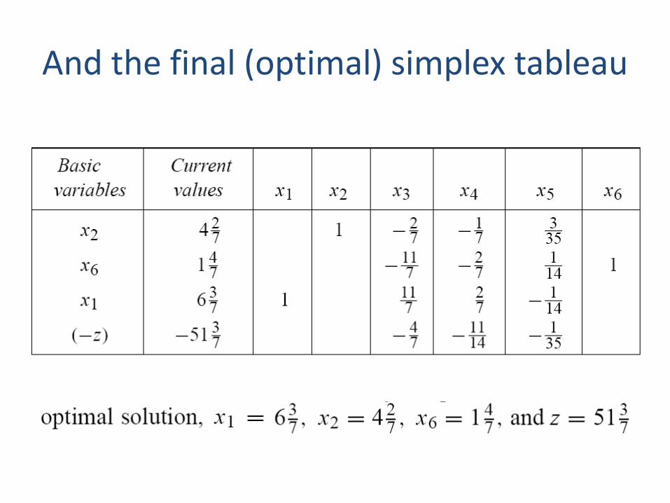
And the final (optimal) simplex tableau

Aims

• We wish to analyze the effect on the optimal solution of changing various elements of the problem data without re-solving the linear program or having to remember any of the intermediate tableaus generated in solving the problem by the simplex method.

• The type of results that can be derived in this way are conservative, in the sense that they provide sensitivity analysis for changes in the problem data small enough so that the same decision variables remain basic, but not for larger changes in the data.

SHADOW PRICES, REDUCED COSTS AND NEW ACTIVITIES

Shadow prices

• Definition. The shadow price associated with a particular constraint is the change in the optimal value of the objective function per unit increase in the righthand-side value for that constraint, all other problem data remaining unchanged.

• Suppose that the production capacity in the first constraint of our model is increased from 60 to 61 hours:

• Solving a new problem with 1 unit more on the right-hand side is algebraically equivalent to allow the slack variable x4 to take on the negative value of -1 in the original problem.

• How does the objective function changes when x4 is replaced by x4 − 1 (i.e., from its optimal value x4 = 0 to x4 = −1)?

• In the optimal solution x3 = x4 = x5 = 0 because they are nonbasic variables.

• If now x4 = −1, the profit increases by 11/14 hundred dollars the shadow price

• The shadow price for a particular constraint is merely the negative of the coefficient of the appropriate slack (or artificial) variable in the objective function of the final tableau.

• Shadow prices are associated with the constraints of the problem and not the variables.

• For our example, the shadow prices are 11/14 hundred dollars per hour of production capacity, 1/35 hundred dollars per hundred cubic feet of storage capacity, and zero for the limit on six-ounce juice-glass demand.

Reduced costs

• Definition. The reduced cost associated with the nonnegativity constraint for each variable is the shadow price of that constraint (i.e., the corresponding change in the objective function per unit increase in the lower bound of the variable).

• The reduced costs can also be obtained directly from the objective equation in the final tableau:

• Increasing the righthand side of x3 ≥ 0 by one unit to x3 ≥ 1 forces champagne glasses to be used in the final solution. Therefore, the optimal profit decreases by −4/7.

• Increasing the righthand sides of x1 ≥ 0 and x2 ≥ 0 by a small amount does not affect the optimal solution, so their reduced costs are zero.

• In every case, the shadow price for the nonnegativity constraint on a variable (reduced cost of the variable) is the objective coefficient for this variable in the final canonical form. For basic variables, these reduced costs are zero.

Pricing out an activity

• The operation of determining the reduced cost of an activity from the shadow price and the objective function is generally referred to as pricing out an activity.

• In this view, the shadow prices are thought of as the opportunity costs associated with diverting resources away from the optimal production mix.

Example with variable x3

• Since the new activity of producing champagne glasses requires 8 hours of production capacity per hundred cases, whose opportunity cost is 11/14 hundred dollars per hour, and 10 hundred cubic feet of storage capacity per hundred cases, whose opportunity cost is 1/35 hundred dollars per hundred cubic feet, the resulting total opportunity cost of producing one hundred cases of champagne glasses is:

• Now the contribution per hundred cases is only 6 hundred dollars so that producing any champagne glasses is not as attractive as producing the current levels of six-ounce juice glasses and ten-ounce cocktail glasses.

• Therefore, if resources were diverted from the current optimal production mix to produce champagne glasses, the optimal value of the objective function would be reduced by 4/7 hundred dollars per hundred cases of champagne glasses produced. This is exactly the reduced cost associated with variable x3.

Generalization

Objective function in the optimal solution

Shadow prices

Relationship between shadow prices, reduced costs and the problem data

• Recall that, at each iteration of the simplex method, the objective function is transformed by subtracting from it a multiple of the row in which the pivot was performed.

• Consequently, the final form of the objective function could be obtained by subtracting multiples of the original constraints from the original objective function.

Relationship between shadow prices, reduced costs and the problem data

• Consider first the final objective coefficients associated with the original basic variables xn+1, xn+2, . . . , xn+m and let π1, π2, . . . , πn be the multiples of each row that are subtracted from the original objective function to obtain its final optimal form.

• Since xn+i appears only in the ith constraint and has a +1 coefficient, we should have:

which, combined with means that The shadow prices yi are the multiples πi

The multiples can be used to obtain every objective coefficient in the final form.

• Since for the m basic variables of the optimal solution, we

have: • This is a system of m equations in m unknowns that

uniquely determines the values of the shadow prices yi .

VARIATIONS IN THE OBJECTIVE COEFFICIENTS

Variations in the objective coefficients

• How much the objective-function coefficients can vary without changing the values of the decision variables in the optimal solution?

• We will make the changes one at a time, holding all other coefficients and righthand-side values constant.

Variation of objective coefficient of x3, a nonbasic variable in our example

• Suppose that we increase the objective function coefficient of x3 in the original problem formulation by ∆c3:

• In applying the simplex method, multiples of the rows were subtracted from the objective function to yield the final system of equations.

• Therefore, the objective function in the final tableau will remain unchanged except for the addition of ∆c3 x3.

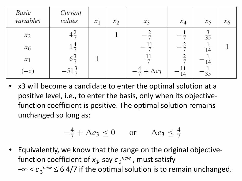
• x3 will become a candidate to enter the optimal solution at a positive level, i.e., to enter the basis, only when its objective-function coefficient is positive. The optimal solution remains unchanged so long as:

• Equivalently, we know that the range on the original objective-function coefficient of x3, say c 3

new , must satisfy −∞ < c 3

new ≤ 6 4/7 if the optimal solution is to remain unchanged.

Variation of objective coefficient of x1, a basic variable in our example

• Suppose now that we increase the objective function coefficient of x1 in the original problem formulation by ∆c1:

• As x1 is basic, this tableau is not canonical and therefore a pivot operation has to be made.

• In order to have the current solution remain unchanged:

• Taking the most limiting inequalities, the bounds on ∆c1 are:

• If we let c 1new = c1 + ∆c1 be the objective-

function coefficient of x1 in the initial tableau, then:

Which variables will enter and leave the basis when the new cost coefficient reaches either

of the extreme values of the range?

• When c 1new = 5 2/5:

– the objective coefficient of x5 in the final tableau becomes 0; thus x5 enters the basis for any further increase of c 1

new – by the usual ratio test of the simplex method

variable x6 leaves the basis:

• When c 1new = 4 7/11:

– the objective coefficient of x3 in the final tableau becomes 0; thus x3 enters the basis for any further decrease of c 1

new – by the usual ratio test of the simplex method

variable x1 leaves the basis.

VARIATIONS IN THE RIGHTHAND-SIDE VALUES

Overview

• When changing a righthand-side, the values of the decision variables are clearly modified!

• But any change in the righthand-side values that keep the current basis, and therefore the canonical form, unchanged has no effect upon the objective-function coefficients.

• Consequently, the righthand-side ranges are such that the shadow prices and the reduced costs remain unchanged for variations of a single value within the stated range.

Varying the righthand-side value for the demand limit on six-ounce juice glasses

• If we add an amount ∆b3 to the righthand side of this constraint, the constraint changes to:

• x1 is nonbasic (equal to zero) and x6 was basic in the initial tableau and is basic in the optimal tableau, therefore x6 is merely increased or decreased by ∆b3. In order to keep the solution feasible:

• This implies that: or, equivalently, that:

Varying the righthand-side value for the storage-capacity constraint

• If we add an amount ∆b2 to the righthand side of this constraint, the constraint changes to:

• This is equivalent to decreasing the value of the slack variable x5 of the corresponding constraint by ∆b2; that is, substituting x5 − ∆b2 for x5 in the original problem formulation.

• In this case, x5, which is zero in the final solution, is changed to x5 = − ∆b2.

• Making these substitutions in the final tableau provides the following relationships:

• In order for the current basis to remain optimal, it need only remain feasible, since the reduced costs will be unchanged by any such variation in the righthand-side value:

which implies:

⇔

All these computations can be carried out directly in terms of the final tableau…

• When changing the ith righthand-side by ∆bi , we simply substitute −∆bi for the slack variable in the corresponding constraint and update the current values of the basic variables accordingly:

Example for ∆b2

Variable transitions

• When changing demand on six-ounce juice glasses, we found that the basis remains optimal if b 3

new ≥ 6 3/7 and that for b 3new < 6 3/7 , the

basic variable x6 becomes negative. • In the later case x6 has to leave the basis, since

otherwise it would become negative. • What variable would then enter the basis to take

its place? In order to have the new basis be an optimal solution, the entering variable must be chosen so that the reduced costs are not allowed to become positive.

• Regardless of which variable enters the basis, the entering variable will be isolated in row 2 of the final tableau to replace x6 , which leaves the basis.

• To isolate the entering variable, we must perform a pivot operation, and a multiple, say t, of row 2 in the final tableau will be subtracted from the objective-function row.

• Assuming that b 3new were set equal to 6 3/7 in

the initial tableau the final tableau would be:

• In order that the new solution be an optimal solution, the coefficients of the variables in the objective function of the final tableau must be nonpositive:

⇓

• Since the coefficient of x3 is most constraining on t, x3 will enter the basis. Note that the range on the righthandside value and the variable transitions that would occur if that range were exceeded by a small amount are easily computed.

• However, the pivot operation actually introducing x3 into the basis and eliminating x6 need not be performed.

ALTERNATIVE OPTIMAL SOLUTIONS AND SHADOW PRICES

Alternative optimal solutions

• As in the case of the objective function and righthand-side ranges, the final tableau of the linear program tells us something conservative about the possibility of alternative optimal solutions…

• If all reduced costs of the nonbasic variables are strictly negative (positive) in a maximization (minimization) problem, then there is no alternative optimal solution, because introducing any variable into the basis at a positive level would reduce (increase) the value of the objective function.

• If one or more of the reduced costs are zero, there may exist alternative optimal solutions.

Example

• x3 could be introduced into the basis without changing the value of the objective function.

• By the minimum ratio x1 leaves the basis. • The alternative optimal solution is then found by

completing the pivot that introduces x3 and eliminates x1.

Alternative shadow prices

• Independent of the question of whether or not alternative optimal solutions exist in the sense that different values of the decision variables yield the same optimal value of the objective function, there may exist alternative optimal shadow prices.

• If all righthand-side values in the final tableau are positive, then there do not exist alternative optimal shadow prices.

• If one or more of these values are zero, then there may exist alternative optimal shadow prices.

Example

• Since the righthand-side value in row 2 is zero, it is possible to drop x6 (basic variable in row 2) from the basis as long as there is a variable to introduce into the basis.

• The variable to be introduced into the basis can be determined from the entering variable condition: