CHAPTER-3 DETRENDED FLUCTUATION ANALYSIS OF FINANCIAL TIME...
22
41 CHAPTER-3 DETRENDED FLUCTUATION ANALYSIS OF FINANCIAL TIME SERIES
Transcript of CHAPTER-3 DETRENDED FLUCTUATION ANALYSIS OF FINANCIAL TIME...

41
CHAPTER-3
DETRENDED FLUCTUATION ANALYSIS OF
FINANCIAL TIME SERIES

42
3.1 Introduction
Detrended Fluctuation Analysis (DFA) has been established as an
important tool for the detection of long range autocorrelations in time-series
with non-stationarities, which often affects experimental data. DFA is a
method for determining the scaling behavior of data in the presence of possible
trends without knowing their origin & shape. It has been applied to diverse
field of DNA , heart rate dynamics , human gait , long-time weather records ,
cloud structure , economical time-series etc.
Consider a time-series τi , where i = 1,2,3,……..N and N is the length of
the series. To implement DFA method the steps below are followed:
The series is first integrted to obtain the cumulative time series
y(k) = τ- τ ) where k = 1,2,3,4,…….N (3.1)
Here τ indicates the mean interevent time &
k
i
i
1
Breaking up y(k) into T non-overlapping time intervals , It of equal size
r, where t = 0,1,2,………….T-1 & T corresponds to the integer part of N/r.
The local trend function
Yr(k) = at + btk for k ε It (3.2)
Where the coefficients at & bt represents the least-square linear fit of
y(k) in interval It.
The rescaled function
k
i 1
(

43
Where s = data standard deviation
The Hurst exponent H is then obtained from the scaling behavior of F(r)
F(r) = CrH
(3.5)
Where C = constant, independent of time lag r
H = Hurst scaling exponent
Here Hurst exponent H represents the slope of the straight line graph of
log F(r) to log r . Typically F(r) increases with r.
In double logarithmic plot of log F(r) v/s log r graph although the slope
of straight line gives the Hurst exponent H. In practical problem H depends on
the choice of the interval within which the linear fit is performed.
To overcome this problem, F(r) may be written such that
FH (r) = CH rH
(3.6)
Where, CH =
2
1
1
2
2
1
12
2
HHH
(3.7)
The above equation gives a one parameter estimator for the Hurst
exponent H, so that we can adjust H simply to obtain the best arrangement
between the theoretical curve predicted by FH(r) & the empirical data for
F(r).The scaling exponent, correlation exponent α quantify the correlation
properties of the signal. It can have different values
α <1/2 Anti correlated
44
α ≈ 1/2 UN correlated
α > 1/2 Correlated
α ≈1 1/f noise
α >1 Non stationary random walk
α ≈ 3/2 Brownian motion
Many physical systems do not obey conventional scaling laws. Broad
probability distributions are characteristics for such observables, for instance
the growing probability in DLA (Diffusion limited aggregation) the
distribution of voltage loss in random resister network or the probability
dentition random walks on fractals [1, 2, 3,].
In all cases the moment of the distribution can‟t be characterized by a
single exponent. So the scaling behavior in non-trivial for different values of q
= 1, 2, 3… This phenomenon was described for the first time by B.B.
Mandelbrot in 1970. Today it is known as multi fractality. The original
meaning of multi fractal leads to the question about the processes that create
multi fractal structure. The multiplicative cascaded of random processes create
multi fractal structure, while additive processes generally produce simple
fractals (mono fractals). Multi fractals are used to describe & distinguish
varieties of complicated figure, system & processes in nature.
Many algorithms have been developed to measure the multi fractal
dimerism. The method to calculate multi fractal spectra was proposed by T. C.
Halsey in 1986. In this method multi fractal spectra for quantities of states of a
system with a random fractal character can be calculated.

45
The nature of price fluctuation in stock markets has been of interest to
the traders as well as a variety of professionals for a long time. A large
numbers of methods have been applied to characterize the time evaluation of
stock price and stock market indices. The correlation properties of stock prices
can be described using DFA.
3.2 Result of Analysis
The DFA analysis was performed for the data sets and the results
obtained are as follows: The Index values and volumes with its DFA profiles
are plotted at different time. Figure 3.1 shows the NSE Index daily closing
values from 12.08.2002 to 25.08.2010. Figure3.2 shows DFA profile for the
same NSE Index daily closing values from 12.08.2002 to 25.08.2010. Figure
3.3 is the DFA profile for NSE Index monthly closing values from 12.08.2002
to 25.08.2010. Figure 3.4 shows the DFA profile for NSE Index quarterly
closing values from 12.08.2002 to 25.08.2010.Figure 3.5 is the Graph for
trading volume of Japanese stock market Index NIKKEI(volume) from 21st
Jul.2009 to30th
Dec.2012 .Figure 3.6 shows the DFA profile for NIKKEI
volume. Fig 3.7.shows the Graph of NIKKEI Adjusted closing value Y(n). Fig
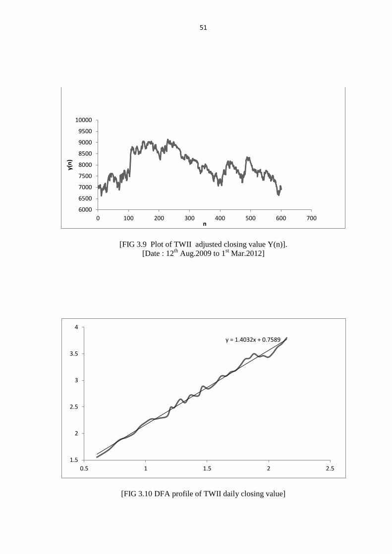
3.8 shows the DFA profile for NIKKEI Adjusted closing value Y(n). Fig 3.9
shows Graph for Taiwan stock market index TWII (Adjusted closing value
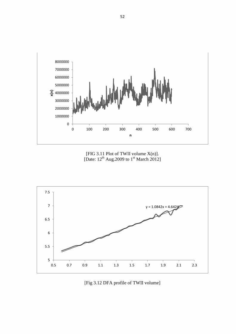
Y(n). Figure 3.10 is a plot of DFA profile for TWII closing value. Fig 3.11
shows the Graph of TWII (volume) X(n) from 12th
Aug.2009 to 1st Mar.2012.
Figure 3.12 is the plot of DFA profile for TWII volume. Figure 3.13 shows the
Graph of STI Adjusted closing value no. of data point (n) and data point
Y(n)] from 1st Sep.2009 to 1
st Mar.2012. Figure 3.14 is the plot of DFA profile
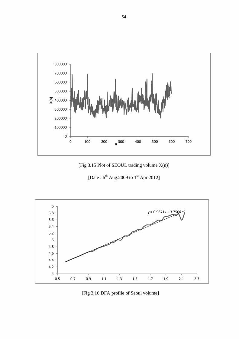
for STI closing value Figure 3.15 shows the Graph of SEOUL stock market
index volume X(n) from 6th
Aug.2009 to 1st Apr.2012. Figure 3.16 is the plot
of DFA profile for Seoul volume. Figure 3.17 shows the Graph of trading
volume of German stock market index DAX from 9th Apr.2009 to 1
st

46
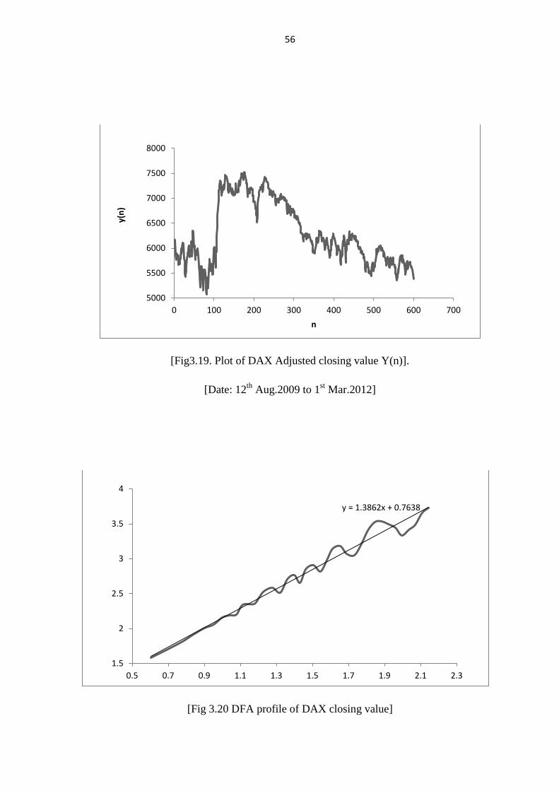
Apr.2012. Figure 3.18 is the DFA profile for DAX volume. Fig3.19 shows the
Graph of DAX (Adjusted closing value) Y(n) from 1st Mar.2012 to 12
th
Aug.2009.Figure 3.20 is the DFA profile for DAX closing value. Figure 3.21
shows the Graph of DOW-JONES Industrial Average (Adjusted closing value)
from 1st Mar.2012 to 27
th Aug.2009. Fig 3.22 is the plot of DFA profile for
DOW-JONES Industrial average adjusted closing value.
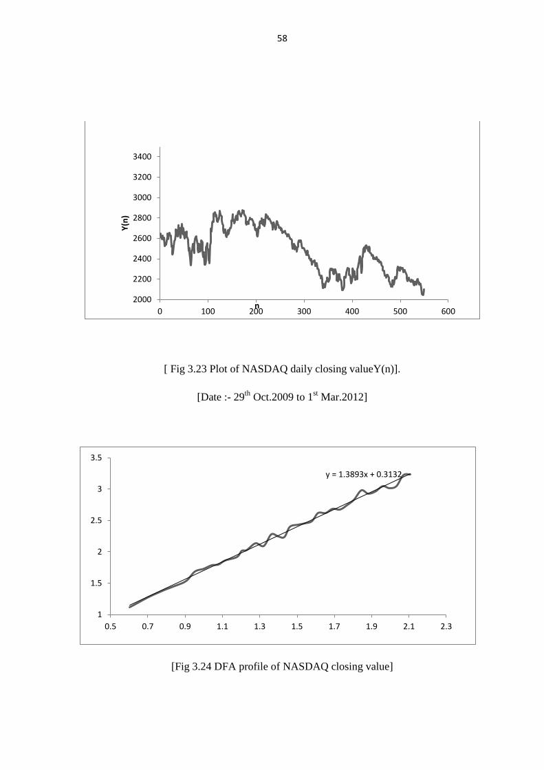
Figure 3.23 shows the Graph of NASDAQ Adjusted closing value Y(n)
from 1st Mar.2012 to 29
th Oct.2009. Figure 3.24 is the plot of DFA profile for
NASDAQ Adjusted closing value. Fig 3.25 shows the Graph of NASDAQ
trading volume X(n) from 1st Mar.2012 to 29
th Oct.2009. Figure 3.26 is the
plot of DFA profile for NASDAQ volume.

47
[FIG 3.1 NSE index daily closing values from 12.08.2002 to 12.08.2011]
[FIG 3.2 DFA profile for NSE index daily closing values from 12.08.2002 to 12.08.2011]
0 0.5
1 1.5
2 2.5
3 3.5
4 4.5
5
0 0.5 1 1.5 2 2.5 3 Ln N
Ln F(N)
0
1000
2000
3000
4000
5000
6000
7000
0 500 1000 1500 2000
48
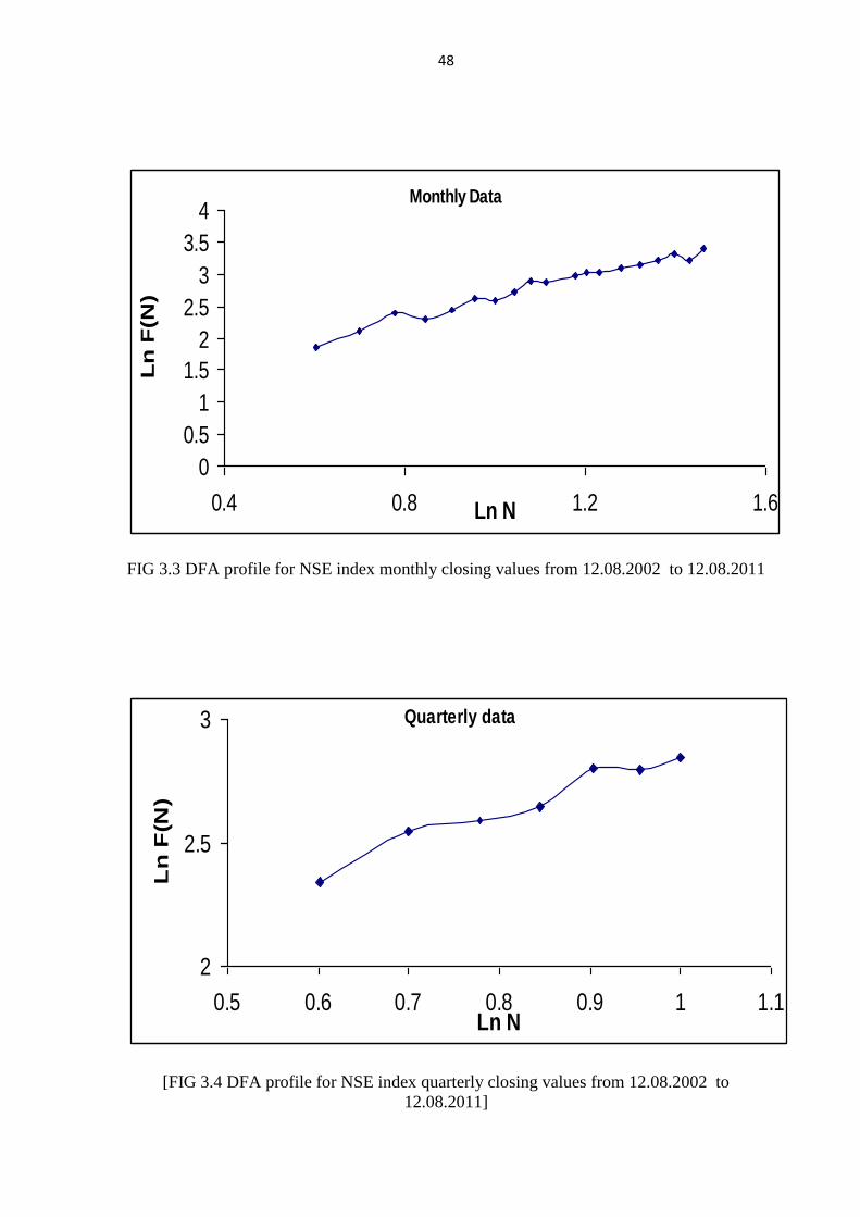
FIG 3.3 DFA profile for NSE index monthly closing values from 12.08.2002 to 12.08.2011
[FIG 3.4 DFA profile for NSE index quarterly closing values from 12.08.2002 to
12.08.2011]
Monthly Data
0
0.5
1
1.5
2
2.5
3
3.5
4
0.4 0.8 1.2 1.6Ln N
Ln
F(N
)
Quarterly data
2
2.5
3
0.5 0.6 0.7 0.8 0.9 1 1.1Ln N
Ln
F(N
)
49
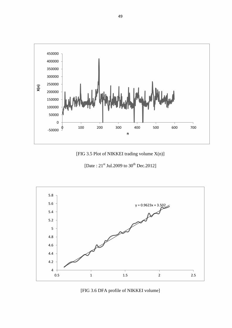
[FIG 3.5 Plot of NIKKEI trading volume X(n)]
[Date : 21st Jul.2009 to 30
th Dec.2012]
[FIG 3.6 DFA profile of NIKKEI volume]
-50000
0
50000
100000
150000
200000
250000
300000
350000
400000
450000
0 100 200 300 400 500 600 700
X(n
)
n
y = 0.9623x + 3.502
4
4.2
4.4
4.6
4.8
5
5.2
5.4
5.6
5.8
0.5 1 1.5 2 2.5

50
[FIG 3.7 Plot of NIKKEI Adjusted closing value Y(n)]
[Date : 21st Jul.2009 to 30
th Dec.2012]
[FIG 3.8 DFA profile of NIKKEI closing value]
8000
10000
0 100 200 300 400 500 600 700
Y(n
)
n
y = 1.3855x + 0.9248
2
2.5
3
3.5
4
4.5
0.5 1 1.5 2 2.5
51
[FIG 3.9 Plot of TWII adjusted closing value Y(n)].
[Date : 12th
Aug.2009 to 1st Mar.2012]
[FIG 3.10 DFA profile of TWII daily closing value]
6000
6500
7000
7500
8000
8500
9000
9500
10000
0 100 200 300 400 500 600 700
y(n
)
n
y = 1.4032x + 0.7589
1.5
2
2.5
3
3.5
4
0.5 1 1.5 2 2.5
52
[FIG 3.11 Plot of TWII volume X(n)].
[Date: 12th
Aug.2009 to 1st March 2012]
[Fig 3.12 DFA profile of TWII volume]
0
1000000
2000000
3000000
4000000
5000000
6000000
7000000
8000000
0 100 200 300 400 500 600 700
x(n
)
n
y = 1.0842x + 4.6424
5
5.5
6
6.5
7
7.5
0.5 0.7 0.9 1.1 1.3 1.5 1.7 1.9 2.1 2.3

53
[Fig 3.13 Plot of STI adjusted closing value Y(n)]
[Date: 1st Sep.2009 to 1
st Mar.2012]
[Fig 3.14. DFA profile of STI closing value]
2500
3000
0 100 200 300 400 500 600 700
Y(n
)
n
y = 1.3999x + 0.25
1
1.5
2
2.5
3
3.5
0.5 0.7 0.9 1.1 1.3 1.5 1.7 1.9 2.1 2.3
54
[Fig 3.15 Plot of SEOUL trading volume X(n)]
[Date : 6th
Aug.2009 to 1st Apr.2012]
[Fig 3.16 DFA profile of Seoul volume]
0
100000
200000
300000
400000
500000
600000
700000
800000
0 100 200 300 400 500 600 700
X(n
)
n
y = 0.9871x + 3.7506
4
4.2
4.4
4.6
4.8
5
5.2
5.4
5.6
5.8
6
0.5 0.7 0.9 1.1 1.3 1.5 1.7 1.9 2.1 2.3

55
[Fig 3.17 Plot of DAX trading volume X(n)]
[Date : 9th
Apr.2009 to 1st Apr.2012]
[Fig 3.18 DFA profile for DAX volume]
0
20000000
40000000
60000000
80000000
100000000
120000000
140000000
0 100 200 300 400 500 600 700
x(n
)
n
Volume x(n)
y = 0.8311x + 6.232
6.6
6.8
7
7.2
7.4
7.6
7.8
8
8.2
0.5 0.7 0.9 1.1 1.3 1.5 1.7 1.9 2.1 2.3
56
[Fig3.19. Plot of DAX Adjusted closing value Y(n)].
[Date: 12th
Aug.2009 to 1st Mar.2012]
[Fig 3.20 DFA profile of DAX closing value]
5000
5500
6000
6500
7000
7500
8000
0 100 200 300 400 500 600 700
y(n
)
n
y = 1.3862x + 0.7638
1.5
2
2.5
3
3.5
4
0.5 0.7 0.9 1.1 1.3 1.5 1.7 1.9 2.1 2.3

57
[ Fig 3.21 Plot of DJIA adjusted closing value Y(n)].
[Date: 27th
Aug.2009 to 1st March 2012]
[Fig 3.22 DFA profile of DJIA closing value]
9000
9500
10000
10500
11000
11500
12000
12500
13000
13500
14000
0 100 200 300 400 500 600 700 800
y(n
)
n
y = 1.4205x + 0.8294
1.5
2
2.5
3
3.5
4
4.5
0.5 1 1.5 2 2.5
58
[ Fig 3.23 Plot of NASDAQ daily closing valueY(n)].
[Date :- 29th
Oct.2009 to 1st Mar.2012]
[Fig 3.24 DFA profile of NASDAQ closing value]
2000
2200
2400
2600
2800
3000
3200
3400
0 100 200 300 400 500 600
Y(n
)
n
y = 1.3893x + 0.3132
1
1.5
2
2.5
3
3.5
0.5 0.7 0.9 1.1 1.3 1.5 1.7 1.9 2.1 2.3

59
[ FIG 3.25 plot of NASDAQ trading volume X(n)]
[Date: 29th
Oct. to 1st Mar.2012]
[FIG 3.26 DFA profile of NASDAQ trading volume]
0
500000000
1E+09
1.5E+09
2E+09
2.5E+09
3E+09
3.5E+09
4E+09
4.5E+09
5E+09
0 100 200 300 400 500 600
X(n
)
n
y = 0.9265x + 7.5732
8
8.2
8.4
8.6
8.8
9
9.2
9.4
9.6
9.8
0.5 0.7 0.9 1.1 1.3 1.5 1.7 1.9 2.1 2.3

60
3.3 Discussion:
The scaling properties of different time series were calculated using
detrended fluctuation analysis. The daily closing value of indices were
considered the till 26th sep. 2010. Dataset of NIFTY contains 2015 data
points where as DAX data contains 4991 and DJIA data contains 5262 data
points. The week-ends and holidays are not considered. The data were
collected from the website of yahoo finance [9].
By using DFA analysis, the fractal dimension of NSE index for daily,
monthly, and quarterly closing values are calculated. The variation of DFA
function values of NIFTY index with n shows that data follows simple scaling
behavior. Almost same result is obtained for daily closing values of DAX and
DJIA indices .Since the value of slope is found to be near to 1.5, for all types
of data sets with small variance, the market behavior shows nearly classical
Brownian random walk. But it is important to note that we have used closing
values of Indices only. It will be interesting to look for mono/multifractal
features in short term (single day data, but intra-day behavior).
This study offers the advantage of a means to investigate long range
correlations within a financial signal due to the intrinsic properties of the
system producing the signal, rather than external stimuli unrelated to the
properties of the system. In addition, the calculation is based on the entire data
set and is 'scale free', offering greater potential to distinguish signals based on
scale specific measures. Theoretically, the scaling exponent varies from 0.5
(random numbers) to 1.5 (random walk). A scaling exponent greater than 1.0
indicates a loss in long range scaling behavior r and an alteration in the
underlying system. The technique was initially applied to detect long range
correlations in DNA sequences but has been increasingly applied to financial

61
time signals. [5,10,11]. DFA is not very much affected due to nonstationariety
of data. Although DFA represents a novel technological development in the
science of variation analysis and has proven its significance, whether it offers
information distinct from traditional spectral analysis is debated [11]. It is
inappropriate to simply 'run' the DFA algorithm blindly on data sets. Finally,
although appealing in order to simplify comparison, the calculation of two
scaling exponents (one for small and one for large n) represents a somewhat
arbitrary manipulation of the results of the analysis. The assumption that the
same scaling pattern is present throughout the signal remains flawed, and
therefore techniques without this assumption are being developed and are
referred to as multifractal analysis.
62
3.4 References
[1]. Giovani L. Vasconcelos, Brazilian Jr. of Phys., vol. 34, 3B, 1039(2004)
[2]. E.F.Fama, J. finance 45, 1089 (1990)
[3]. B.B. Mandelbrot, ,/. Husincsa 36, 349 (1963)
[4]. E.E.Peters, Fractal Market Analysts, (Wiley, New York, 1994)
[5].. N.Vandewalle and M .Ausloos, Physica A 240, 454 (1997)
[6]. Ashok Razdan, ,Pramana, Vol. 58, No. 3 , pp. 537–544(March 2002)
[7] Hurst, H.E., Black, R.P. and Simaika, Y.M. Long-Term Storage: An
Experimental Study. Constable, London.xiv,145 p (1965).
[8 ] Peng C-K, Buldyrev SV, Havlin S, Simons M, Stanley HE, Goldberger
AL. Phys Rev E;49:1685-1689. (1994); Peng C-K, Havlin S, Stanley
HE, Goldberger AL. Chaos 5:82-87(1995).
[9]. http://in.finance.yahoo.com/
[10]. Balgopal Sharma, Study of the Multifractal behavior of NIFTY using
Detrended Fluctuation Analysis, ECONOPHYS-KOLKATA V:
International Workshop on Econophysics of order driven markets, 9-13
(March 2010). http://www.saha.ac.in/cmp/epkol 05.2010/abstracts.html.
[11]. Ravi Sharma, B.G. Sharma, D.P. Bisen and Malti Sharma, STUDY OF
SCALING BEHAVIOR OF NIFTY USING DETRENDED
FLUCTUATION ANALYSIS, Econophysics Colloquium 2010 , in
Taipei, Taiwan(November 4-6, 2010).