Chapter 3 PROBABILITY. Chapter 3 3.1 – EXPLORING PROBABILITY.
Upload
garry-gautamaCategory
view
213download
0
28
Chapter 3
Molecular dynamics study on reaction and motion
of misfit dislocation on Ni/Ni3Al interface
3.1 Introduction
Although the QC can treat the microstructure in the submicron-scale, however, it
is limited in the “two dimensional” modeling due to the computational cost. As same as
the usual FEM, the computation drastically increases if we treat directly three
dimensional models. In the two dimensional modeling, the dislocation is represented as
“point defect” and the core interaction is only “annihilation”. On the other hand, the
dislocations show complex behavior in the three dimensional space. Thus we shift our
focus on the detail of misfit dislocations at γ/γ’ interface, from the strain field of the real
microstructure. Although a misfit dislocation definitely exists as lattice strain at the
interface, it doesn’t mean that the γ or γ’ phase has an extra or a missing of an atomic
plane. If we assume the interface as a slip plane, the motion of misfit dislocation can be
evaluated according to the dislocation theory; however, the dislocation theory based on
the standard continuum approach fails to consider the change of the atomic structure at
the interface, such as the interaction between misfit core and approaching dislocation
gliding in monoatomic lattice. Several reports [45,70,71] have proposed semi-coherent
misfit dislocation model in a periodic simulation cell. The structure of dislocation core,
the shape and deformation under external loading, and the interaction with prismatic
dislocation loop emitted from a spherical punch have been reported [70,71]. It is
difficult, however, to clarify the detail of the interaction between misfit dislocation with
gliding one in the γ phase, since many dislocations with complicated characters
(Burgers vector) produced in a small simulation cell. In this chapter, we use the same
simulation cell but inject simple edge or screw dislocations into the γ phase, and
Chapter 3. Molecular dynamics study on reaction and motion of misfit dislocation 29
bumped them into the misfit dislocation at the semi-coherent interface. The detail of the
crossing mechanism between dislocation cores will be discussed. Then we simulate
shear loading in the [100] and [110] direction by applying an atomic displacement at the
top and bottom surface of the same cell. The behavior of the network at the interface
will be analyzed.
3.2 Basic theory for MD simulation
3.2.1 MD outline
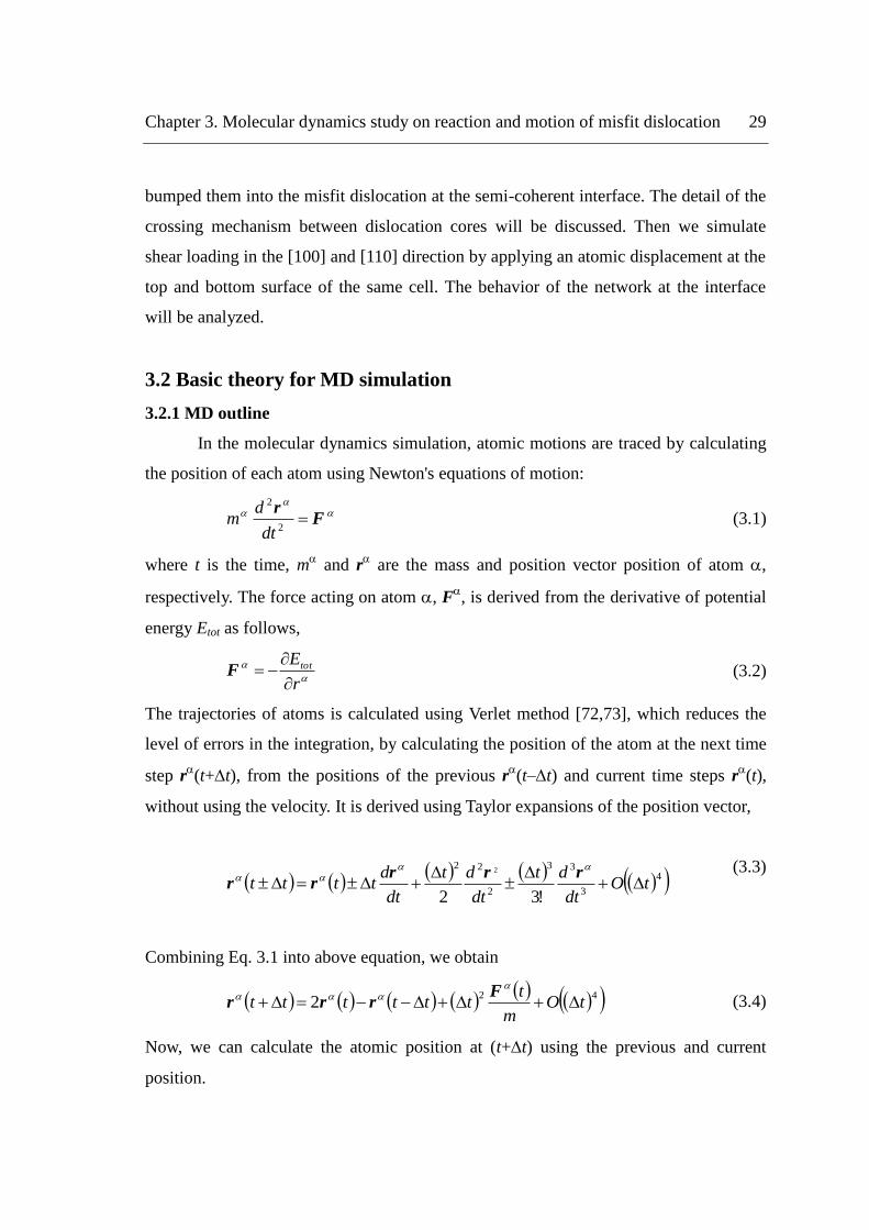
In the molecular dynamics simulation, atomic motions are traced by calculating
the position of each atom using Newton's equations of motion:
F
r
2
2
dt
dm (3.1)
where t is the time, m and r
are the mass and position vector position of atom ,
respectively. The force acting on atom , F, is derived from the derivative of potential
energy Etot as follows,
r
Etot
F (3.2)
The trajectories of atoms is calculated using Verlet method [72,73], which reduces the
level of errors in the integration, by calculating the position of the atom at the next time
step r(t+t), from the positions of the previous r
(t–t) and current time steps r
(t),
without using the velocity. It is derived using Taylor expansions of the position vector,
4
3
33
2
22
!32
2
tOdt
dt
dt
dt
dt
dtttt
rrr
rr (3.3)
Combining Eq. 3.1 into above equation, we obtain
422 tO
m
ttttttt
F
rrr (3.4)
Now, we can calculate the atomic position at (t+t) using the previous and current
position.

Chapter 3. Molecular dynamics study on reaction and motion of misfit dislocation 30
3.2.2 Interatomic potential
Same as the previous QC simulation, the embedded atom method (EAM) is used
in the MD simulation. The total energy, Etot, is evaluated by
ttttot Fr
2
1E (3.5)
with
rt (3.6)
where r is the scalar distance between atom and , is the pair wise interaction
between atoms, F is the “embedding function” of , the “density” at atom , that
is given by the superposition of another pair wise interaction, r , from neighboring
atoms. t and t indicate the types of atoms and respectively.
In fitting an alloy potential, linear transformation is applied so that
gFF (3.7)
rg2rr (3.8)
and scaling transformation is also applied to the density as
rsr (3.9)
sFF (3.10)
with g and s are the linear and scaling transformation parameter, and the prime indicates
the transformed function.
In fitting the pure element, the density of a hydrogenic 4s orbital is taken as the
density function
r29r6 e2err
(3.11)
where is an adjustable parameter. Morse type potential is taken as the pair wise
interaction with
1Rrexp1Dr2
MMM (3.12)

Chapter 3. Molecular dynamics study on reaction and motion of misfit dislocation 31
where DM, RM, and M define the depth, position of the minimum, and the curvature at
the minimum of the energy curve, respectively. After linear and scaling transformations
have been applied, we have
r29r6 e2esrr
(3.13)
rg21Rrexp1Dr2
MMM (3.14)
To ensure that the interatomic potential and its first derivatives are continues,
both r and r are smoothly cut of at r = rcut by using the following function
cut
m
cut
cutcutsmooth
rrdr
dh
r
r1
m
rrhrhrh
(3.15)
Here, h(r) = r or r with m = 20. F is derived from the Rose’s relation
between crystal lattice expansion and sublimation energy of the universal energy
function [67]. This is then fitted into the cubic spline function, in the range of
0 0.1 with the spline knots at intervals of 010. .
Table 3.1: Potential parameters for (r) [65].
-1Å s
Ni
Al
3.6408
3.3232
1.0
0.6172
Table 3.2: Potential parameter for (r) [65].
D (eV) (Å-1
) R (Å) g (eV Å3)
Ni-Ni
Al-Al
Ni-Al
1.5335
3.7760
3.0322
1.7728
1.4859
1.6277
2.2053
2.1176
2.0896
6.5145
-0.2205
0

Chapter 3. Molecular dynamics study on reaction and motion of misfit dislocation 32
3.2.3 Velocity scaling
In the present study, temperature of the system is controlled by velocity scaling
method. The temperature T is directly related to the kinetic energy, K, expressed by
TNkmK B
N
2
3
2
1
1
vv (3.16)
where m and v
are the mass and the velocity of atom , respectively. N is the total
number of atoms in the system, and kB is Boltzmann constant. To calculate the
temperature, above equation can be described as
BNk
mT
3
vv
(3.17)
Considering a constant temperature, TC, and T as instantaneous temperature of the
system after velocity update. Eq. (3.17) indicates that if we scale the particle velocity, v,
by a constant TTC , thus the system will be at temperature TC. Then using the Verlet
method we scale the integration of Eq. (3.4) as follows:
2t
m
tttt
T
Tttt C
F
rrrr (3.18)
3.3 Simulation procedure
3.3.1 Misfit dislocation on a semi-coherent interface
As shown in Fig. 3.1(a), a cell is built by stacking Ni3Al phase contains
49x49x35 of L12 lattice on a 50x50x35 lattice cell of Ni phase. The total number of
atoms is 686,140 atoms. At the initial arrangement, the lattice parameter of γ and γ’
phase are set to 0.3498 nm and 0.3570 nm, respectively (so that 50aγ = 49aγ’), to avoid
misfit concentration at the interface. The periodic boundary is set only in the x and y

Chapter 3. Molecular dynamics study on reaction and motion of misfit dislocation 33
directions, while free surface in the z direction. By controlling the length of the cell in
the x and y direction, the normal stress is cancelled during initial relaxation of 15000 fs.
Although superalloys are used in high temperature, the temperature is set to 10 K in the
present simulation to avoid the complication of the effect of temperature and strain.
After the initial relaxation, misfit dislocation is formed at the interface, as shown in
Fig.3.1(b). In the figure, only the atoms in the γ’ phase and the “defect”, or the atoms
neither fcc nor hcp judged by Common neighbor analysis (CNA) [68], are drawn. The
network contains two kinds of edge dislocations which are aligned in the [110] and
]101[ direction. The Burgers vector of each dislocation is b⊥ = a/2 ]101[ and b// =
a/2 ]011[ , respectively. Here a is the average lattice spacing.
50 fcc
50 fcc lattices (Ni)(17.6 nm)
49 L1 lattices(Ni Al) (17.6 nm)
2
3
49 L1 2
35
lat
tice
s(1
2.6
nm
)3
5 l
atti
ces
(12
.3 n
m)
‘
[010] [100]
[001]
tt//
b
b//
(a) Cell dimensions (b) Line and Burgers vectors
of misfit dislocation
Fig. 3.1: Dimension of simulation cell and network dislocation nucleated after initial
relaxation.
Chapter 3. Molecular dynamics study on reaction and motion of misfit dislocation 34
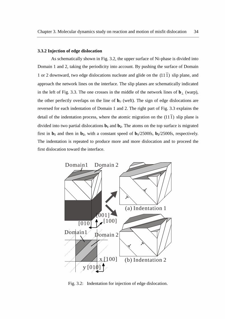
3.3.2 Injection of edge dislocation
As schematically shown in Fig. 3.2, the upper surface of Ni-phase is divided into
Domain 1 and 2, taking the periodicity into account. By pushing the surface of Domain
1 or 2 downward, two edge dislocations nucleate and glide on the )111( slip plane, and
approach the network lines on the interface. The slip planes are schematically indicated
in the left of Fig. 3.3. The one crosses in the middle of the network lines of b⊥ (warp),
the other perfectly overlaps on the line of b// (weft). The sign of edge dislocations are
reversed for each indentation of Domain 1 and 2. The right part of Fig. 3.3 explains the
detail of the indentation process, where the atomic migration on the )111( slip plane is
divided into two partial dislocations b1 and b2. The atoms on the top surface is migrated
first in b1 and then in b2, with a constant speed of b1/2500fs, b2/2500fs, respectively.
The indentation is repeated to produce more and more dislocation and to proceed the
first dislocation toward the interface.
Domain1 Domain 2
(a) Indentation 1
(b) Indentation 2
Domain1Domain 2
y [010]
[001]
x [100]
[010] [100]
Fig. 3.2: Indentation for injection of edge dislocation.

Chapter 3. Molecular dynamics study on reaction and motion of misfit dislocation 35
3.3.3 Injection of screw dislocation
Even if we apply relative shear by shifting Domain 1 against Domain 2, we
cannot generate screw dislocation at the border of Domain 1 and 2 but edge dislocation
in the other slip plane. Thus we apply the local shear at the border lines between the
domains. According to the black and white gradation in Fig. 3.4(a), the magnitude of
atoms displacement is controlled. At the surface of Domain 2, the displacement of two
partial dislocations, b3 and b4, are given during 5000 fs. On the other hand, the atoms in
the dark part of Domain 1 are migrated in b5 = a/6[112] for 2500 fs and returned in b6 =
a/6 ]211[ for 2500 fs. This control is decayed in the white side and no displacement
control is given at the border of white and black in Fig. 3.4(a). Due to the relative
displacement at the border of Domain 1 and 2, this process leads the resulting migration
of b7 and b8 in the white side.
Dislocation Network
b//
b//b
b
Atoms on the upper slip plane
Atoms on the lower slip plane
b= a
2[101]
b =1
a
6[112]
[101]
b =2
a
6[211]
Fig. 3.3: Slip plane and displacement control for injection of edge dislocations.

Chapter 3. Molecular dynamics study on reaction and motion of misfit dislocation 36
3.3.4 Shear simulation in [100] and [110] direction
As schematically shown in Fig. 3.5(a), the atom motion in the top surface of Ni
phase and the bottom surface of Ni3Al phase of the simulation cell is controlled as
chucks in the shear simulation. The width is 0.350 nm and 0.357 nm for Chuck 1 and 2,
respectively. The relative displacement in the [100] and ]001[ are applied on each
chuck. For the [110] shear, the atom coordinate is transformed to orient the x and y axes
to [110] and ]101[ , respectively, under the periodic boundary condition. The
displacement dux is defined as,
Domain 1 Domain 2A A
[010] [001]
[100]
Domain 1 Domain 2
[010]
[100]
Plane A-A
(a) Domain of upper surface.
b =4
a
6211[ ] b =8
a
621 1[ ]
b =3
a
621[ ]1 b =7
a
6211[ ]
b4 b3b5,b =6 a
6[112]
(b) Atom migration control at the surface. (c) Resulting migration.
Fig. 3.4: Displacement control for injection of screw dislocations.

Chapter 3. Molecular dynamics study on reaction and motion of misfit dislocation 37
tantan2
1 dzzdux (3.18)
where dux and are displacement and engineering strain, respectively, as explained in
Fig. 3.5(b) in the case of [100] simulation. The dux in both simulations is changed every
step in order to set the strain rate d to constant value of 1.0×10⁻⁶
[1/fs] = 1.0×10⁹
[1/s].
3.4 Results and discussion
3.4.1 Indentation simulation 1
Snapshots of dislocation motion under the indentation of Domain 1 are shown in
Fig. 3.6. Here only the defect (dislocation core) and hcp atoms in the leading and
trailing partials are shown by CNA; and the camera angle is rotated from the previous
figures. As shown in Fig. 3.6(a) of t = 9000 fs, the dark shaded atoms of stacking fault
can be seen between the core of leading and trailing partials (light shaded ones). In this
report, the dislocations on the slip plane overlapping the network line are referred as
zz
Chuck 2
Chuck 1
[010]
[001]
[100]
dux
d
[001]
[100]
zz
(a) Controlled domain (b) Shear displacement in [100]
Fig. 3.5: Shear simulation procedure.

Chapter 3. Molecular dynamics study on reaction and motion of misfit dislocation 38
Dislocation A, while the others crossing normal to the network lines as Dislocation B. If
the line vector is defined from reader’s direction, the Burgers vector of Dislocation A
and B are bA = -(b1+b2), and bB = -bA, respectively.
First, we discuss the overlapping collision between Dislocation A and network
line. In Fig. 3.6(d), Dislocation A reaches to the network line at t = 12000 fs. Here we
can see that another dislocation overlaps to the network in the left of the figure. This
dislocation is not an image of the right Dislocation A by periodic boundary condition,
but a different part of the same dislocation. In the next figure, Fig. 3.6(e), the stacking
fault are found on the conjugate slip plane )111( , and its leading partial goes up to the
upper right direction in Fig. 3.6(f).
Figure 3.7 shows the detail of the change of slip plane during 11700–12900 fs.
The first leading partial stops at the position of the network line (Fig. 3.7(a)). The width
of the extended dislocation narrows, and the core begins to nucleate on the conjugate
)111( slip plane from the position of the network line (Fig. 3.7(b)), then expands into
]211[ and opposite ]211[ direction (Fig. 3.7(c)). Finally it becomes an extended
dislocation on the (111) plane (Fig. 3.7(d) and (e)) and moves away from the interface
as shown in Figs. 3.6(f)-(i). Eventually Dislocation A bounces at the interface. Here, the
Burgers vector of the reflecting Dislocation A’, bA’, is the sum of the Burgers vector of
Dislocation A, bA, and that of misfit dislocation, b//. The reaction of Burgers vector is
shown in Fig. 3.6(f) by arrows. During t = 14000-15000 fs, the trailing partial of the
second Dislocation B2 unites with the leading partial of Dislocation A’. Then the trailing
partial on the interface breaks off from the position of original network line and finally
misfit dislocation disappears from the interface (Figs. 3.6(h) and (i)).
Now we discuss the perpendicular collision between Dislocation B and network
line in Fig. 3.6. The leading partial of Dislocation B is pulled into the network at t =
10000 fs and bows its shape. Its width and curve become smaller as it receives repulsive
force from the following Dislocation B2 (Fig. 3.6 (c) and (d)). Figure 3.6(j) shows a top
view of the dislocation at t = 15000 fs. Misfit dislocation slightly shifts as pointed by
arrows in the middle of the figure. To observe the detail of the crossing process, the
dislocation structure at t =14000 fs is magnified in Fig. 3.8. Figures 3.8(b) and (c) show

Chapter 3. Molecular dynamics study on reaction and motion of misfit dislocation 39
the crossing process with tilted angles from the network line of Fig. 3.8(d). We can see a
delta-roof-like expansion of misfit dislocation in Fig. 3.8(c), since two leading partials
nucleate from the misfit dislocation on the )111( and )111( slip planes. These slip
planes are not parallel to that of Dislocation B, so that the dislocations show
complicated morphology on the different slip planes. Figure 3.9 shows the schematic of
Dislocation B Dislocation A
Trailingpartial
Leadingpartial
bA
bB
bA’ bA
(a) t = 9000 fs (b) t = 10000 fs (c) t = 11000 fs (d) t = 12000 fs (e) t = 13000 fs
(f) t = 14000 fs (g) t = 15000 fs (h) t = 16000 fs (i) t = 17000 fs (j) t = 15000 fs, top view
b//
B2 A2
Fig. 3.6: Snapshots of dislocations in indentation of Domain 1.
3D view
Side view
(a) 11700 fs (b) 12000 fs (c) 12300 fs (d) 12600 fs (e) 12900 fs
[112]
[112]
Fig. 3.7 Slip plane change of Dislocation A.

Chapter 3. Molecular dynamics study on reaction and motion of misfit dislocation 40
the slip planes and the Burgers vector of the partial dislocations. The atomic migration
by Dislocation B are divided into the leading and trailing partials of b1 and b2 as shown
in upper left in Fig. 3.9(a). The leading partials take place on the delta-roof slip planes
in Fig. 3.9(a) and the Burgers vectors are a/6 ]211[ in the left side and a/6 ]211[ in the
right, respectively. Both of them doesn’t coincide with b1; however, in the left side of
the roof, the Burgers vector of “perfect dislocation” coincide with bB = a/2 ]101[ , by
the trailing partial of a/6 ]112[ on the roof. The Burgers vector of the leading partial of
Dislocation B, b1, is a/6 ]211[ while the trailing on the left roof is a/6 ]112[ . Although
the vectors do not perfectly match each other, all of the values are negative and the
directions are close. It’s also same for the relation between the trailing of Dislocation B,
b2 = a/6 ]112[ , and the nucleated leading of a/6 ]211[ on )111( plane. Therefore, as
shown in the left side of network line in Fig. 3.9(b), the former and latter combinations
make continuous line, respectively, and can penetrate into Ni3Al phase by shifting the
intersection point on the cross sectional lines between )111( and )111( planes. On the
other hand, the leading partial on the right roof is formed by bowing out from the
network line and intersections between the slip plane of Dislocation B and the right
roof; however, the Burgers vector never match with that of Dislocation B, even if the
trailing partial nucleated on the right roof of )111( slip plane. Therefore they can’t
develop any more.
[001]
[110][110]
[001]
[110]
[110]
[001]
[110][110]
Misfit dislocation
Misfit dislocation
Misfit dislocation
Dislocation B
(c)
(d)
(b)
(b) Rotated view 1(a) View point (c) Rotated view 2 (d) [110] view
Fig. 3.8: Magnified view of dislocations in Fig. 3.6(f).

Chapter 3. Molecular dynamics study on reaction and motion of misfit dislocation 41
3.4.2 Indentation simulation 2
Figure 3.10 shows the snapshots of dislocations under the indentation of
Domain 2. Similar with the previous section, Dislocation A is the one that collides in
parallel with the network line, while Dislocation B crosses perpendicularly. First, we
discuss the behavior of Dislocation A. The leading partial of Dislocation A reaches
misfit dislocation at t = 12000 fs, as shown in the left and right in Fig. 3.10(b). Here, we
can see the stripe pattern of the dislocation core and stacking fault (SF) in the left in
Fig. 3.10(b). Thus, contrary to the previous Indentation 1, the leading edge easily passes
the interface and penetrates into the γ’ phase. On the other hand, the right part of
Dislocation A is slightly late to reach the network, and don’t show the stripe pattern but
wavy form in Figs. 3.10(c) and (d). Carefully observed, the delta-roof-like leading
partials emerges in the intersection between the left stripe and the warp (b⊥ ) as
indicated by arrows in Figs. 3.10(c) and (d). The wavy shape of the right part of
Dislocation A is due to such complicated dislocation relationship. Then, according to the
force from approaching Dislocation A2, the intersection of the delta-roof and the SF in
the stripe pattern dissolve and the front end of dislocation proceeds into the γ’ phase
bB
b =B
a
2[101]
b =1
a
6[112] (111)
b =2
a
6[211]
a
6[112]
a
6[211]
(111)
[010]
[001]
[100]
(111)
b =
a
2[110]
bBbB
b =B
a
2[101]
b =
a
2[110]
b =1
a
6[112]
b =2
a
6[211]
a6
[112]
a
6[211]
a
6[112]
b =1
a6
[112]
b2
b
(a) Slip planes (b) Burgers vector
Fig. 3.9: Schematic of slip planes and Burgers vectors in Fig. 3.8(c).

Chapter 3. Molecular dynamics study on reaction and motion of misfit dislocation 42
(indicated by the circle in Figs. 3.10.(g)-(j)). Figure 3.11 shows the magnification of the
change during t = 15000–18000 fs. Figure 3.11(a) illustrates the camera position and
angle. In the upper-right in Fig. 3.11(b), we can see the following Dislocation A2 “cut
off” by periodic simulation cell. The stripe pattern still remains in Fig. 3.11(b) at t =
15000 fs, then the front end proceeds into the ’ phase as if a hole nucleated and
expanded from the center line of the stripe (Figs. 3.11(c)–(e)). Here, we can see that the
delta-roof enlarges and the cross point shift on the intersection line of the slip planes, as
same as the mechanism previously explained in Fig. 3.9(b). On the other hand,
separated dislocation is left on the interface as can be seen in the middle of Fig. 3.11(e),
and glides on the interface. Figure 3.12 shows the top view of the dislocation
morphology near the interface by eliminating dislocations more than 1.25 nm far from
the interface. As indicated in Fig. 3.12(a), two cells are displayed to show the
connection of dislocation lines under the periodic boundary condition. The intersection
previously explained in Fig. 3.11 locates in the center of the cell (Arrow 1 in Fig.
3.12(b)). We can see the dislocation glides on the interface and change the network
morphology (Arrow 1 in Figs. 3.12.(b)–(e)). Same change can be observed in the other
intersection as indicated by Arrow 2 in Fig. 3.12(c).
bAbB
(a) = 11000 fst (b) = 12000 fst (c) = 13000 fs t (d) = 14000 fst (e) = 15000 fst
(f) = 16000 fst (g) = 17000 fst (h) = 18000 fst (i) = 19000 fst (j) = 20000 fst
B2 A2
A
B
Fig. 3.10: Snapshots of dislocations under indentation of Domain 2.

Chapter 3. Molecular dynamics study on reaction and motion of misfit dislocation 43
Now, let’s go back to Fig. 3.10 and discuss the behavior of Dislocation B.
Contrary to the indentation of Domain 1, Dislocation B is pinned at the warp of the
network lines and hardly proceed into the γ’ phase until the following Dislocation B2
comes very close. Figure 3.13 shows Dislocation B in the [110] direction (along the
warp) under Indentation 1 and 2. In the previous Indentation 1, the intersection part
shrunks while it remains extended in Indentation 2. Moreover, there is no nucleation of
leading partial from the warp, or the delta-roof-like nucleation, in Fig. 3.13.(b).
Summarizing the collision of edge dislocations in Indentation 1 and 2, the delta-
roof-like dislocations nucleate from misfit network and penetrates into γ’ phase, by
Dislocation B in Indentation 1, and by Dislocation A in Indentation 2. In the both cases,
there is an extra atomic plane above the slip plane, considered as same sign with the
misfit dislocation which has also an extra atomic plane in the γ side as schematically
shown in Fig. 3.14(a). On the other hand, the reflection of Dislocation A in
Indentation 1 and the pinning of Dislocation B in Indentation 2 have opposite sign
against network line. Thus the Burgers vector reaction occurs through out the line in the
former case, while point locks occur in the latter one.
(a) View point
1
(b) = 15000 fst (c) = 16000 fst (d) = 17000 fst (e) = 18000 fst
2
A2
Fig. 3.11: Dissociation from the junction between misfit dislocation node and
approaching edge dislocation.
A A
A
B
B
Periodicboundary 1
2
2
1 1 1
(c) t = 18000 fs(b) t = 17000 fs(a) t = 16000 fs (d) t = 19000 fs (e) t = 20000 fs
Fig. 3.12: Morphology change of dislocations on the interface (Indentation 2).

Chapter 3. Molecular dynamics study on reaction and motion of misfit dislocation 44
(a) Indentation 1 (b) Indentation 2
Fig. 3.13: Magnified view of edge dislocations crossing over the warp of misfit
dislocations.
A B
On the line Cross the line
(a) Same sign
A B
On the line Cross the line
(b) Opposite sign
Fig. 3.14: Schematic explanation for interaction between misfit dislocation and edge
dislocation.

Chapter 3. Molecular dynamics study on reaction and motion of misfit dislocation 45
3.4.3 Injection of screw dislocation
Figure 3.15 shows the dislocation motion in the simulation cell. Similar with the
previous notation, Dislocation A collides with network line in parallel while
Dislocation B does in vertical. First, we discuss the behavior of Dislocation A. In Fig.
3.15(c), Dislocation A reaches the network line. At the same time a leading partial
generates on the conjugate slip plane and bounces like a reflection at the mirror. Figure
3.16 shows the comparison between the change of slip plane in Indentation 1 and the
reflection of this screw dislocation, by showing the collision from the viewpoint parallel
to the interface and approaching dislocation lines. The previous edge dislocation
changes the slip plane by incorporating with misfit dislocation and expanding the
leading and trailing partials on the conjugate slip plane around the original position of
misfit dislocation. On the other hand, the leading partial directly changes the slip plane
and reflects at the interface, in the case of screw dislocation in Fig. 3.16(b). In Figs.
3.15(f) and (g), the reflected leading partial bump with the leading of second
Dislocation B2, as indicated with the circle in Fig. 3.15(g). The Burgers vector of
(f) = 15000 fst (g) = 16000 fst (h) = 17000 fst (i) = 18000 fst (j) = 19000 fst
(a) = 10000 fst (b) = 11000 fst (c) = 12000 fst (d) = 13000 fst (e) = 14000 fst
(k) = 20000 fst (l) = 21000 fst (m) = 22000 fst (n) = 23000 fst (o) = 24000 fst
bA
bBB2
B A
Fig. 3.15: Snapshots of dislocation in shear simulation for screw dislocation.
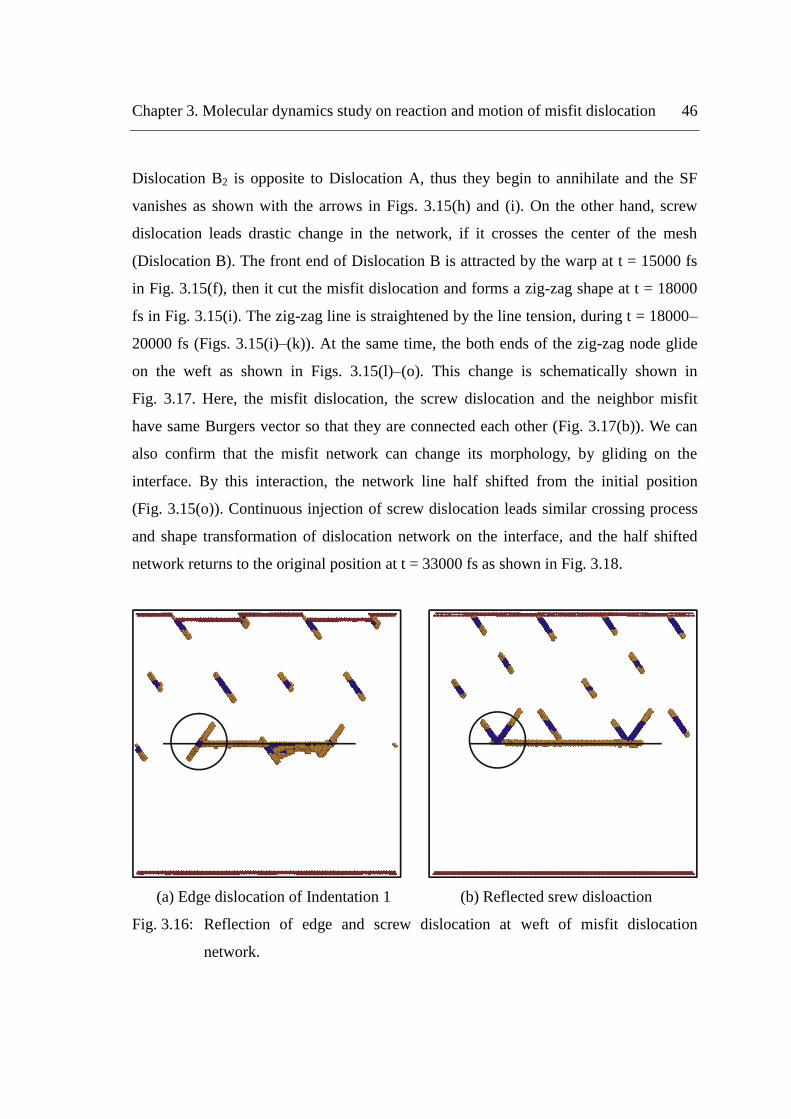
Chapter 3. Molecular dynamics study on reaction and motion of misfit dislocation 46
Dislocation B2 is opposite to Dislocation A, thus they begin to annihilate and the SF
vanishes as shown with the arrows in Figs. 3.15(h) and (i). On the other hand, screw
dislocation leads drastic change in the network, if it crosses the center of the mesh
(Dislocation B). The front end of Dislocation B is attracted by the warp at t = 15000 fs
in Fig. 3.15(f), then it cut the misfit dislocation and forms a zig-zag shape at t = 18000
fs in Fig. 3.15(i). The zig-zag line is straightened by the line tension, during t = 18000–
20000 fs (Figs. 3.15(i)–(k)). At the same time, the both ends of the zig-zag node glide
on the weft as shown in Figs. 3.15(l)–(o). This change is schematically shown in
Fig. 3.17. Here, the misfit dislocation, the screw dislocation and the neighbor misfit
have same Burgers vector so that they are connected each other (Fig. 3.17(b)). We can
also confirm that the misfit network can change its morphology, by gliding on the
interface. By this interaction, the network line half shifted from the initial position
(Fig. 3.15(o)). Continuous injection of screw dislocation leads similar crossing process
and shape transformation of dislocation network on the interface, and the half shifted
network returns to the original position at t = 33000 fs as shown in Fig. 3.18.
(a) Edge dislocation of Indentation 1 (b) Reflected srew disloaction
Fig. 3.16: Reflection of edge and screw dislocation at weft of misfit dislocation
network.

Chapter 3. Molecular dynamics study on reaction and motion of misfit dislocation 47
b
b
b1
2
3
(a) (b)
(c) (d)
Fig. 3.17: Schematic of morphology change in misfit dislocation (shear simulation for
screw dislocation).
Fig. 3.18: Misfit dislocation network at t = 33000 fs (shear simulation for screw
dislocation).

Chapter 3. Molecular dynamics study on reaction and motion of misfit dislocation 48
3.4.4 [100] Shear on the interface
Figure 3.19 shows the relationship between the applied shear strain and the
stress on the simulation cell, while Fig. 3.20 does the corresponding motion of misfit
dislocation. The network does not glide until t = 15000 fs of Fig. 3.20(b), then slowly
shift toward the [100] direction about a half of the cell at t = 30000 fs of Fig. 3.20(c).
After the stress maximum of zx = 3.08 GPa at zx = 0.036, the network begins to flow in
the shear direction, dragging point defects behind the mesh knots (Figs. 3.20(d)–(h)). As
shown in Fig. 3.21, the shear strain absorbed by the slip of the interface, and any
dislocation does not nucleate in γ nor γ’ phase, so that the shape of the and ’ phases
do not change.
Sh
ear
stre
ss
, G
Pa
zx,
Strain, zx
2
1
0
4
0.02 0.04 0.06 0.08
33.08 GPa
Fig. 3.19: Shear stress (zx) against strain under the [100] shear of the interface.

Chapter 3. Molecular dynamics study on reaction and motion of misfit dislocation 49
3.4.5 [110] Shear on the interface
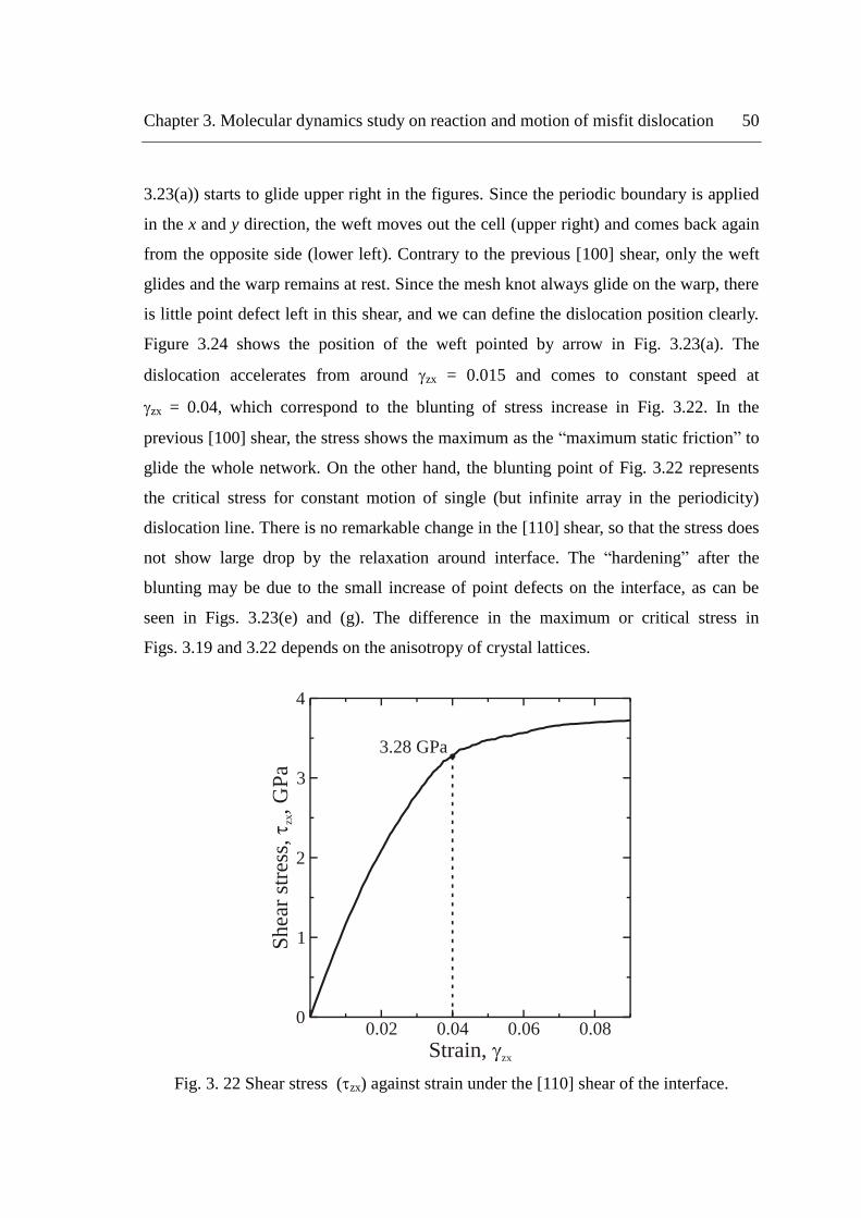
Figure 3.22 shows the stress-strain curve and Fig. 3.23 does the motion of the
network under the [110] shear loading. Compare to Fig. 3.19, the stress-strain curve
does not show definite stress peak, rather shows elastic-plastic behavior with strain
hardening. As same as the previous [100] shear, the network hardly moves until
t = 15000 fs, as can be seen in Figs. 3.23(a) and (b). Then the weft (black arrow in Fig.
(a) = 0 fs, t zx = 0 (b) = 15000 fs, = 0.015t zx (c) = 30000 fs, = 0.03t zx
(e) = 40000 fs, = 0.04t zx (f) = 45000 fs, = 0.045t zx (g) = 50000 fs, = 0.05t zx (h) = 90000 fs, = 0.09t zx
(d) = 36000 fs, = 0.036t zx
[001]
[110]
[110]
Fig. 3.20: Motion of misfit dislocation under the [100] shear on the interface.
[001]
[100][010]
[001]
[100][010]
(a) Side view (b) Rotated view
Fig. 3.21: Analytical cell at t = 90000 fs, zx = 0.09.
Chapter 3. Molecular dynamics study on reaction and motion of misfit dislocation 50
3.23(a)) starts to glide upper right in the figures. Since the periodic boundary is applied
in the x and y direction, the weft moves out the cell (upper right) and comes back again
from the opposite side (lower left). Contrary to the previous [100] shear, only the weft
glides and the warp remains at rest. Since the mesh knot always glide on the warp, there
is little point defect left in this shear, and we can define the dislocation position clearly.
Figure 3.24 shows the position of the weft pointed by arrow in Fig. 3.23(a). The
dislocation accelerates from around zx = 0.015 and comes to constant speed at
zx = 0.04, which correspond to the blunting of stress increase in Fig. 3.22. In the
previous [100] shear, the stress shows the maximum as the “maximum static friction” to
glide the whole network. On the other hand, the blunting point of Fig. 3.22 represents
the critical stress for constant motion of single (but infinite array in the periodicity)
dislocation line. There is no remarkable change in the [110] shear, so that the stress does
not show large drop by the relaxation around interface. The “hardening” after the
blunting may be due to the small increase of point defects on the interface, as can be
seen in Figs. 3.23(e) and (g). The difference in the maximum or critical stress in
Figs. 3.19 and 3.22 depends on the anisotropy of crystal lattices.
Sh
ear
stre
ss
, G
Pa
zx,
Strain, zx
2
1
0
4
0.02 0.04 0.06 0.08
3
3.28 GPa
Fig. 3. 22 Shear stress (zx) against strain under the [110] shear of the interface.

Chapter 3. Molecular dynamics study on reaction and motion of misfit dislocation 51
( = 0 fs, = 0ta) ( ) = 15000 fs, = 0.015tb ( = 25000 fs, = 0.025tc)
( = 42500 fs, = 0.0425te) ( = 50000 fs, = 0.05tf) ( = 55000 fs, = 0.055tg) ( = 90000 fs, = 0.09th)
( = 35000 fs, = 0.035td)
[001]
[110]
[110]
Fig. 3.23: Motion of misfit dislocation under the [110] shear of the interface.
80
60
40
20
0
Po
siti
on
, ,
nm
d
Strain, zx0.02 0.04 0.06 0.08
16.1 nm
Fig. 3.24: Position of the dislocation in Fig. 3.22(a) against strain.

Chapter 3. Molecular dynamics study on reaction and motion of misfit dislocation 52
3.5 Conclusion
Many molecular dynamics simulations are implemented to clarify the reaction
and motion of misfit dislocations on a semi-coherent Ni/Ni3Al interface. First we have
observed carefully the reaction with edge or screw dislocation gliding from Ni-phase.
Overlap on the network line and point collision by crosscutting are considered as well
as the sign of Burgers vectors. It is revealed that the reaction can be basically explained
by the Burgers vectors equation, e.g. the misfit network and screw dislocation forms a
zig-zag line by crosscutting since the Burgers vector is equal in the misfit (edge) and
screw dislocations. On the other hand, we have also found new mechanisms in the
collision of edge and misfit dislocations with the same sign; delta-roof-like stacking
faults nucleation from the misfit core and gliding mechanism of the edge dislocation
straddling on the intersecting slip planes of the (111) and ( 111 ). Then we have also
applied the [100] and [110] shear on the interface. Under the [100] shear, the network
glides wholly but leaves many defects after the drag of mesh knot. On the other hand,
only the weft of the network glides without leaving defects, under the [110] shear. The
critical stress for the constant slip of the interface is slightly different for the [100] and
[110] shear, due to the anisotropy of the lattices.