Chapter 14 Arbitrary Lagrangian–Eulerian Methods€¦ · dynamics, solid mechanics, and coupled...
25
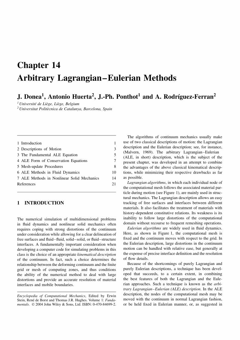
Chapter 14 Arbitrary Lagrangian–Eulerian Methods J. Donea 1 , Antonio Huerta 2 , J.-Ph. Ponthot 1 and A. Rodr´ ıguez-Ferran 2 1 Universit´ e de Li` ege, Li` ege, Belgium 2 Universitat Polit` ecnica de Catalunya, Barcelona, Spain 1 Introduction 1 2 Descriptions of Motion 3 3 The Fundamental ALE Equation 5 4 ALE Form of Conservation Equations 7 5 Mesh-update Procedures 8 6 ALE Methods in Fluid Dynamics 10 7 ALE Methods in Nonlinear Solid Mechanics 14 References 21 1 INTRODUCTION The numerical simulation of multidimensional problems in fluid dynamics and nonlinear solid mechanics often requires coping with strong distortions of the continuum under consideration while allowing for a clear delineation of free surfaces and fluid – fluid, solid – solid, or fluid – structure interfaces. A fundamentally important consideration when developing a computer code for simulating problems in this class is the choice of an appropriate kinematical description of the continuum. In fact, such a choice determines the relationship between the deforming continuum and the finite grid or mesh of computing zones, and thus conditions the ability of the numerical method to deal with large distortions and provide an accurate resolution of material interfaces and mobile boundaries. Encyclopedia of Computational Mechanics, Edited by Erwin Stein, Ren´ e de Borst and Thomas J.R. Hughes. Volume 1: Funda- mentals. 2004 John Wiley & Sons, Ltd. ISBN: 0-470-84699-2. The algorithms of continuum mechanics usually make use of two classical descriptions of motion: the Lagrangian description and the Eulerian description; see, for instance, (Malvern, 1969). The arbitrary Lagrangian–Eulerian (ALE, in short) description, which is the subject of the present chapter, was developed in an attempt to combine the advantages of the above classical kinematical descrip- tions, while minimizing their respective drawbacks as far as possible. Lagrangian algorithms, in which each individual node of the computational mesh follows the associated material par- ticle during motion (see Figure 1), are mainly used in struc- tural mechanics. The Lagrangian description allows an easy tracking of free surfaces and interfaces between different materials. It also facilitates the treatment of materials with history-dependent constitutive relations. Its weakness is its inability to follow large distortions of the computational domain without recourse to frequent remeshing operations. Eulerian algorithms are widely used in fluid dynamics. Here, as shown in Figure 1, the computational mesh is fixed and the continuum moves with respect to the grid. In the Eulerian description, large distortions in the continuum motion can be handled with relative ease, but generally at the expense of precise interface definition and the resolution of flow details. Because of the shortcomings of purely Lagrangian and purely Eulerian descriptions, a technique has been devel- oped that succeeds, to a certain extent, in combining the best features of both the Lagrangian and the Eule- rian approaches. Such a technique is known as the arbi- trary Lagrangian–Eulerian (ALE) description. In the ALE description, the nodes of the computational mesh may be moved with the continuum in normal Lagrangian fashion, or be held fixed in Eulerian manner, or, as suggested in
Transcript of Chapter 14 Arbitrary Lagrangian–Eulerian Methods€¦ · dynamics, solid mechanics, and coupled...
Chapter 14Arbitrary Lagrangian–Eulerian Methods
J. Donea1, Antonio Huerta2, J.-Ph. Ponthot1 and A. Rodrıguez-Ferran2
1 Universite de Liege, Liege, Belgium2 Universitat Politecnica de Catalunya, Barcelona, Spain
1 Introduction 1
2 Descriptions of Motion 3
3 The Fundamental ALE Equation 5
4 ALE Form of Conservation Equations 7
5 Mesh-update Procedures 8
6 ALE Methods in Fluid Dynamics 10
7 ALE Methods in Nonlinear Solid Mechanics 14
References 21
1 INTRODUCTION
The numerical simulation of multidimensional problemsin fluid dynamics and nonlinear solid mechanics oftenrequires coping with strong distortions of the continuumunder consideration while allowing for a clear delineation offree surfaces and fluid–fluid, solid–solid, or fluid–structureinterfaces. A fundamentally important consideration whendeveloping a computer code for simulating problems in thisclass is the choice of an appropriate kinematical descriptionof the continuum. In fact, such a choice determines therelationship between the deforming continuum and the finitegrid or mesh of computing zones, and thus conditionsthe ability of the numerical method to deal with largedistortions and provide an accurate resolution of materialinterfaces and mobile boundaries.
Encyclopedia of Computational Mechanics, Edited by ErwinStein, Rene de Borst and Thomas J.R. Hughes. Volume 1: Funda-mentals. 2004 John Wiley & Sons, Ltd. ISBN: 0-470-84699-2.
The algorithms of continuum mechanics usually makeuse of two classical descriptions of motion: the Lagrangiandescription and the Eulerian description; see, for instance,(Malvern, 1969). The arbitrary Lagrangian–Eulerian(ALE, in short) description, which is the subject of thepresent chapter, was developed in an attempt to combinethe advantages of the above classical kinematical descrip-tions, while minimizing their respective drawbacks as faras possible.
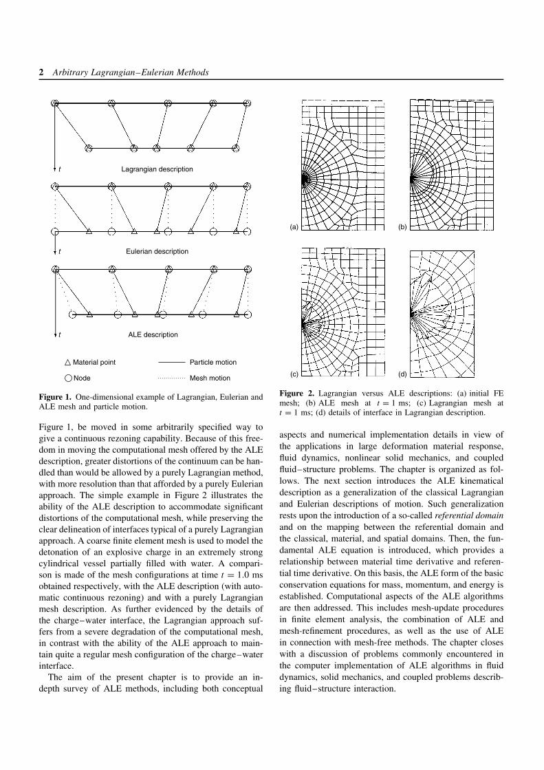
Lagrangian algorithms, in which each individual node ofthe computational mesh follows the associated material par-ticle during motion (see Figure 1), are mainly used in struc-tural mechanics. The Lagrangian description allows an easytracking of free surfaces and interfaces between differentmaterials. It also facilitates the treatment of materials withhistory-dependent constitutive relations. Its weakness is itsinability to follow large distortions of the computationaldomain without recourse to frequent remeshing operations.
Eulerian algorithms are widely used in fluid dynamics.Here, as shown in Figure 1, the computational mesh isfixed and the continuum moves with respect to the grid. Inthe Eulerian description, large distortions in the continuummotion can be handled with relative ease, but generally atthe expense of precise interface definition and the resolutionof flow details.
Because of the shortcomings of purely Lagrangian andpurely Eulerian descriptions, a technique has been devel-oped that succeeds, to a certain extent, in combiningthe best features of both the Lagrangian and the Eule-rian approaches. Such a technique is known as the arbi-trary Lagrangian–Eulerian (ALE) description. In the ALEdescription, the nodes of the computational mesh may bemoved with the continuum in normal Lagrangian fashion,or be held fixed in Eulerian manner, or, as suggested in
2 Arbitrary Lagrangian–Eulerian Methods
t Lagrangian description
t Eulerian description
t ALE description
Material point
Node
Particle motion
Mesh motion
Figure 1. One-dimensional example of Lagrangian, Eulerian andALE mesh and particle motion.
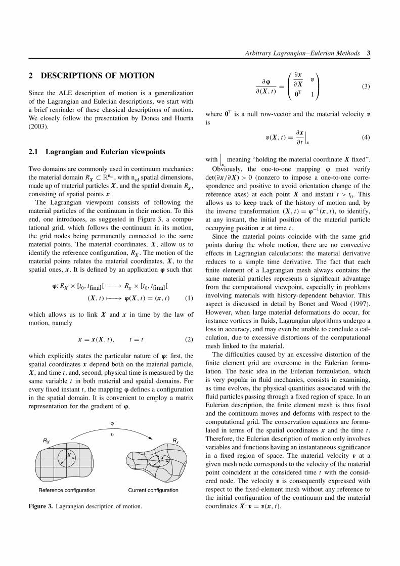
Figure 1, be moved in some arbitrarily specified way togive a continuous rezoning capability. Because of this free-dom in moving the computational mesh offered by the ALEdescription, greater distortions of the continuum can be han-dled than would be allowed by a purely Lagrangian method,with more resolution than that afforded by a purely Eulerianapproach. The simple example in Figure 2 illustrates theability of the ALE description to accommodate significantdistortions of the computational mesh, while preserving theclear delineation of interfaces typical of a purely Lagrangianapproach. A coarse finite element mesh is used to model thedetonation of an explosive charge in an extremely strongcylindrical vessel partially filled with water. A compari-son is made of the mesh configurations at time t = 1.0 msobtained respectively, with the ALE description (with auto-matic continuous rezoning) and with a purely Lagrangianmesh description. As further evidenced by the details ofthe charge–water interface, the Lagrangian approach suf-fers from a severe degradation of the computational mesh,in contrast with the ability of the ALE approach to main-tain quite a regular mesh configuration of the charge–waterinterface.
The aim of the present chapter is to provide an in-depth survey of ALE methods, including both conceptual
(a) (b)
(d)(c)
Figure 2. Lagrangian versus ALE descriptions: (a) initial FEmesh; (b) ALE mesh at t = 1 ms; (c) Lagrangian mesh att = 1 ms; (d) details of interface in Lagrangian description.
aspects and numerical implementation details in view ofthe applications in large deformation material response,fluid dynamics, nonlinear solid mechanics, and coupledfluid–structure problems. The chapter is organized as fol-lows. The next section introduces the ALE kinematicaldescription as a generalization of the classical Lagrangianand Eulerian descriptions of motion. Such generalizationrests upon the introduction of a so-called referential domainand on the mapping between the referential domain andthe classical, material, and spatial domains. Then, the fun-damental ALE equation is introduced, which provides arelationship between material time derivative and referen-tial time derivative. On this basis, the ALE form of the basicconservation equations for mass, momentum, and energy isestablished. Computational aspects of the ALE algorithmsare then addressed. This includes mesh-update proceduresin finite element analysis, the combination of ALE andmesh-refinement procedures, as well as the use of ALEin connection with mesh-free methods. The chapter closeswith a discussion of problems commonly encountered inthe computer implementation of ALE algorithms in fluiddynamics, solid mechanics, and coupled problems describ-ing fluid–structure interaction.
Arbitrary Lagrangian–Eulerian Methods 3
2 DESCRIPTIONS OF MOTION
Since the ALE description of motion is a generalizationof the Lagrangian and Eulerian descriptions, we start witha brief reminder of these classical descriptions of motion.We closely follow the presentation by Donea and Huerta(2003).
2.1 Lagrangian and Eulerian viewpoints
Two domains are commonly used in continuum mechanics:the material domain RX ⊂ R
nsd , with nsd spatial dimensions,made up of material particles X, and the spatial domain Rx ,consisting of spatial points x.
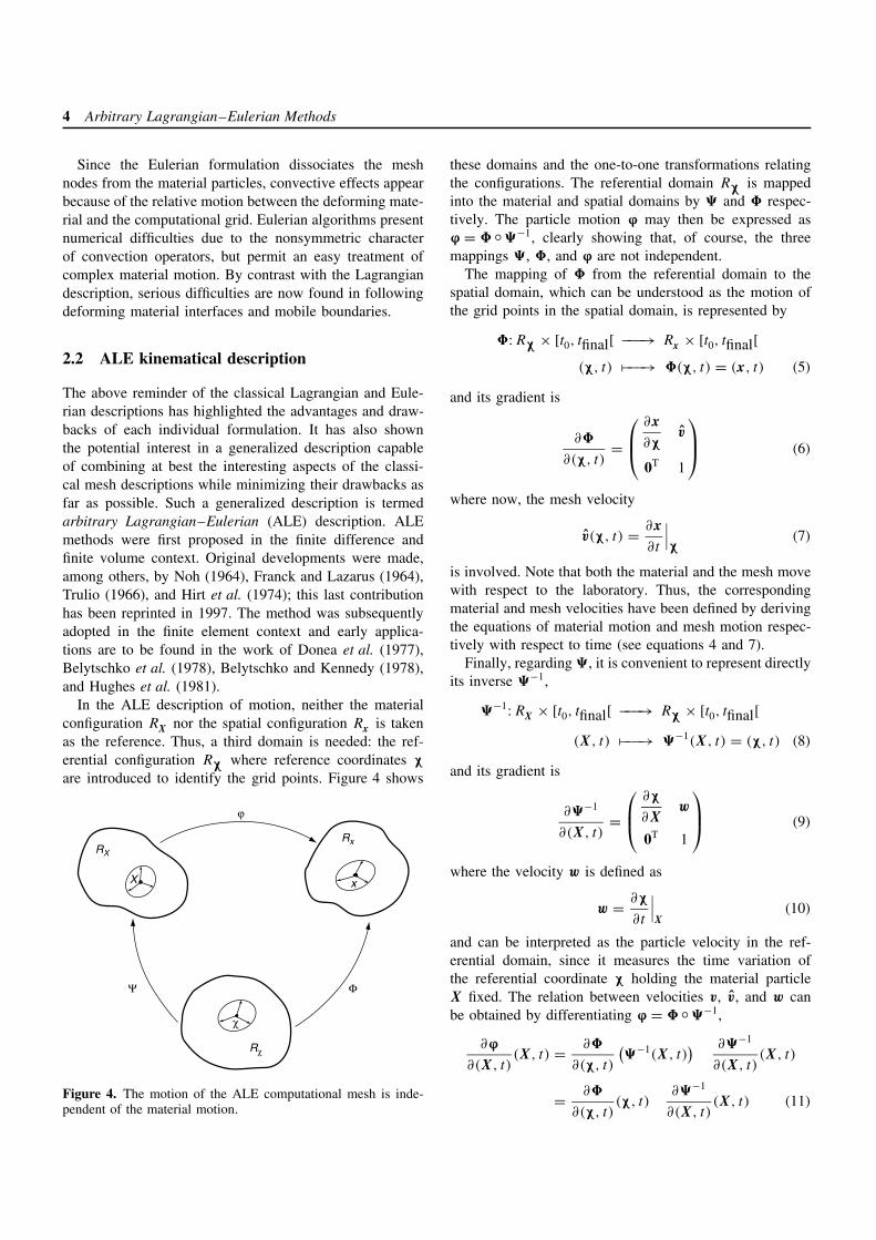
The Lagrangian viewpoint consists of following thematerial particles of the continuum in their motion. To thisend, one introduces, as suggested in Figure 3, a compu-tational grid, which follows the continuum in its motion,the grid nodes being permanently connected to the samematerial points. The material coordinates, X, allow us toidentify the reference configuration, RX . The motion of thematerial points relates the material coordinates, X, to thespatial ones, x. It is defined by an application ϕ such that
ϕ: RX × [t0, tfinal[ −−−→ Rx × [t0, tfinal[
(X, t) �−−−→ ϕ(X, t) = (x, t) (1)
which allows us to link X and x in time by the law ofmotion, namely
x = x(X, t), t = t (2)
which explicitly states the particular nature of ϕ: first, thespatial coordinates x depend both on the material particle,X, and time t , and, second, physical time is measured by thesame variable t in both material and spatial domains. Forevery fixed instant t , the mapping ϕ defines a configurationin the spatial domain. It is convenient to employ a matrixrepresentation for the gradient of ϕ,
ϕ
υRX Rx
Reference configuration Current configuration
xX
Figure 3. Lagrangian description of motion.
∂ϕ
∂(X, t)=
∂x
∂Xv
0T 1
(3)
where 0T is a null row-vector and the material velocity v
is
v(X, t) = ∂x
∂t
∣∣∣x
(4)
with∣∣∣x
meaning “holding the material coordinate X fixed”.
Obviously, the one-to-one mapping ϕ must verifydet(∂x/∂X) > 0 (nonzero to impose a one-to-one corre-spondence and positive to avoid orientation change of thereference axes) at each point X and instant t > t0. Thisallows us to keep track of the history of motion and, bythe inverse transformation (X, t) = ϕ−1(x, t), to identify,at any instant, the initial position of the material particleoccupying position x at time t .
Since the material points coincide with the same gridpoints during the whole motion, there are no convectiveeffects in Lagrangian calculations: the material derivativereduces to a simple time derivative. The fact that eachfinite element of a Lagrangian mesh always contains thesame material particles represents a significant advantagefrom the computational viewpoint, especially in problemsinvolving materials with history-dependent behavior. Thisaspect is discussed in detail by Bonet and Wood (1997).However, when large material deformations do occur, forinstance vortices in fluids, Lagrangian algorithms undergo aloss in accuracy, and may even be unable to conclude a cal-culation, due to excessive distortions of the computationalmesh linked to the material.
The difficulties caused by an excessive distortion of thefinite element grid are overcome in the Eulerian formu-lation. The basic idea in the Eulerian formulation, whichis very popular in fluid mechanics, consists in examining,as time evolves, the physical quantities associated with thefluid particles passing through a fixed region of space. In anEulerian description, the finite element mesh is thus fixedand the continuum moves and deforms with respect to thecomputational grid. The conservation equations are formu-lated in terms of the spatial coordinates x and the time t .Therefore, the Eulerian description of motion only involvesvariables and functions having an instantaneous significancein a fixed region of space. The material velocity v at agiven mesh node corresponds to the velocity of the materialpoint coincident at the considered time t with the consid-ered node. The velocity v is consequently expressed withrespect to the fixed-element mesh without any reference tothe initial configuration of the continuum and the materialcoordinates X: v = v(x, t).
4 Arbitrary Lagrangian–Eulerian Methods
Since the Eulerian formulation dissociates the meshnodes from the material particles, convective effects appearbecause of the relative motion between the deforming mate-rial and the computational grid. Eulerian algorithms presentnumerical difficulties due to the nonsymmetric characterof convection operators, but permit an easy treatment ofcomplex material motion. By contrast with the Lagrangiandescription, serious difficulties are now found in followingdeforming material interfaces and mobile boundaries.
2.2 ALE kinematical description
The above reminder of the classical Lagrangian and Eule-rian descriptions has highlighted the advantages and draw-backs of each individual formulation. It has also shownthe potential interest in a generalized description capableof combining at best the interesting aspects of the classi-cal mesh descriptions while minimizing their drawbacks asfar as possible. Such a generalized description is termedarbitrary Lagrangian–Eulerian (ALE) description. ALEmethods were first proposed in the finite difference andfinite volume context. Original developments were made,among others, by Noh (1964), Franck and Lazarus (1964),Trulio (1966), and Hirt et al. (1974); this last contributionhas been reprinted in 1997. The method was subsequentlyadopted in the finite element context and early applica-tions are to be found in the work of Donea et al. (1977),Belytschko et al. (1978), Belytschko and Kennedy (1978),and Hughes et al. (1981).
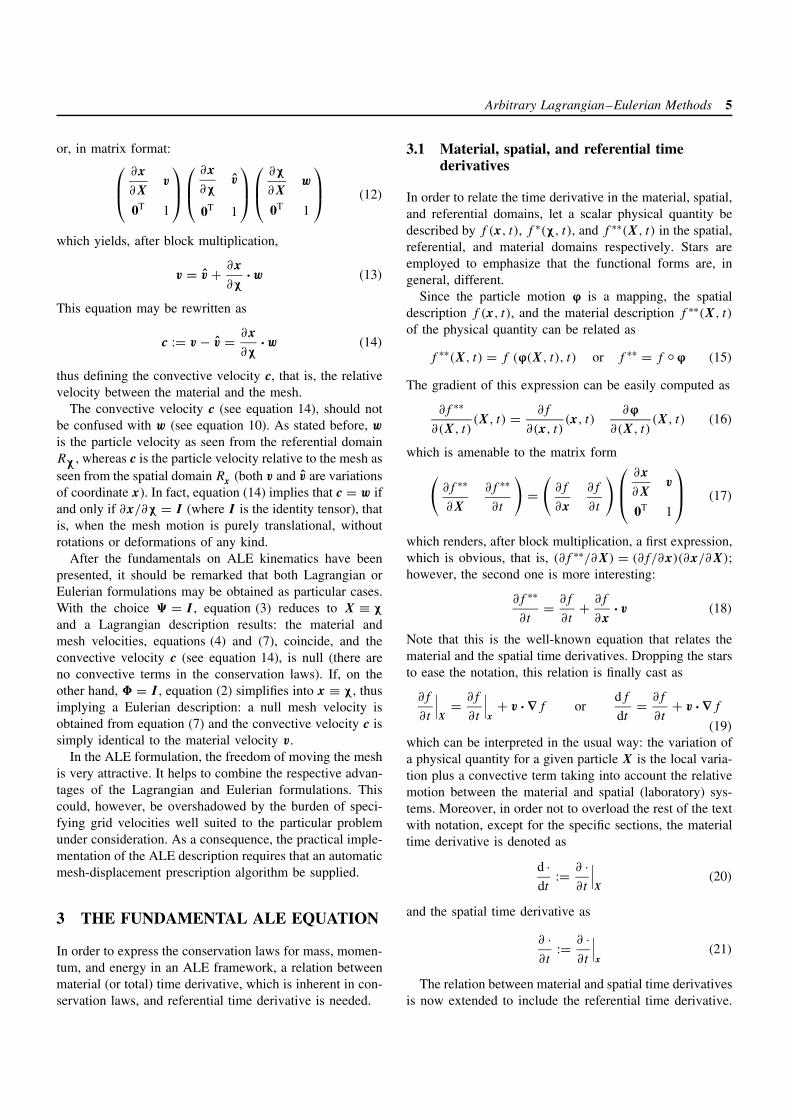
In the ALE description of motion, neither the materialconfiguration RX nor the spatial configuration Rx is takenas the reference. Thus, a third domain is needed: the ref-erential configuration Rχ where reference coordinates χ
are introduced to identify the grid points. Figure 4 shows
Ψ Φ
χ
xX
RX
Rx
Rχ
ϕ
Figure 4. The motion of the ALE computational mesh is inde-pendent of the material motion.
these domains and the one-to-one transformations relatingthe configurations. The referential domain Rχ is mappedinto the material and spatial domains by � and � respec-tively. The particle motion ϕ may then be expressed asϕ = � ◦�−1, clearly showing that, of course, the threemappings �, �, and ϕ are not independent.
The mapping of � from the referential domain to thespatial domain, which can be understood as the motion ofthe grid points in the spatial domain, is represented by
�: Rχ × [t0, tfinal[ −−−→ Rx × [t0, tfinal[
(χ, t) �−−−→ �(χ, t) = (x, t) (5)
and its gradient is
∂�
∂(χ, t)=
∂x
∂χv
0T 1
(6)
where now, the mesh velocity
v(χ, t) = ∂x
∂t
∣∣∣χ
(7)
is involved. Note that both the material and the mesh movewith respect to the laboratory. Thus, the correspondingmaterial and mesh velocities have been defined by derivingthe equations of material motion and mesh motion respec-tively with respect to time (see equations 4 and 7).
Finally, regarding �, it is convenient to represent directlyits inverse �−1,
�−1: RX × [t0, tfinal[ −−−→ Rχ × [t0, tfinal[
(X, t) �−−−→ �−1(X, t) = (χ, t) (8)
and its gradient is
∂�−1
∂(X, t)=
∂χ
∂Xw
0T 1
(9)
where the velocity w is defined as
w = ∂χ
∂t
∣∣∣X
(10)
and can be interpreted as the particle velocity in the ref-erential domain, since it measures the time variation ofthe referential coordinate χ holding the material particleX fixed. The relation between velocities v, v, and w canbe obtained by differentiating ϕ = � ◦ �−1,
∂ϕ
∂(X, t)(X, t) = ∂�
∂(χ, t)
(�−1(X, t)
) ∂�−1
∂(X, t)(X, t)
= ∂�
∂(χ, t)(χ, t)
∂�−1
∂(X, t)(X, t) (11)
Arbitrary Lagrangian–Eulerian Methods 5
or, in matrix format:∂x
∂Xv
0T 1
∂x
∂χv
0T 1
∂χ
∂Xw
0T 1
(12)
which yields, after block multiplication,
v = v + ∂x
∂χ·w (13)
This equation may be rewritten as
c := v − v = ∂x
∂χ·w (14)
thus defining the convective velocity c, that is, the relativevelocity between the material and the mesh.
The convective velocity c (see equation 14), should notbe confused with w (see equation 10). As stated before, w
is the particle velocity as seen from the referential domainRχ, whereas c is the particle velocity relative to the mesh asseen from the spatial domain Rx (both v and v are variationsof coordinate x). In fact, equation (14) implies that c = w ifand only if ∂x/∂χ = I (where I is the identity tensor), thatis, when the mesh motion is purely translational, withoutrotations or deformations of any kind.
After the fundamentals on ALE kinematics have beenpresented, it should be remarked that both Lagrangian orEulerian formulations may be obtained as particular cases.With the choice � = I , equation (3) reduces to X ≡ χ
and a Lagrangian description results: the material andmesh velocities, equations (4) and (7), coincide, and theconvective velocity c (see equation 14), is null (there areno convective terms in the conservation laws). If, on theother hand, � = I , equation (2) simplifies into x ≡ χ, thusimplying a Eulerian description: a null mesh velocity isobtained from equation (7) and the convective velocity c issimply identical to the material velocity v.
In the ALE formulation, the freedom of moving the meshis very attractive. It helps to combine the respective advan-tages of the Lagrangian and Eulerian formulations. Thiscould, however, be overshadowed by the burden of speci-fying grid velocities well suited to the particular problemunder consideration. As a consequence, the practical imple-mentation of the ALE description requires that an automaticmesh-displacement prescription algorithm be supplied.
3 THE FUNDAMENTAL ALE EQUATION
In order to express the conservation laws for mass, momen-tum, and energy in an ALE framework, a relation betweenmaterial (or total) time derivative, which is inherent in con-servation laws, and referential time derivative is needed.
3.1 Material, spatial, and referential timederivatives
In order to relate the time derivative in the material, spatial,and referential domains, let a scalar physical quantity bedescribed by f (x, t), f ∗(χ, t), and f ∗∗(X, t) in the spatial,referential, and material domains respectively. Stars areemployed to emphasize that the functional forms are, ingeneral, different.
Since the particle motion ϕ is a mapping, the spatialdescription f (x, t), and the material description f ∗∗(X, t)
of the physical quantity can be related as
f ∗∗(X, t) = f (ϕ(X, t), t) or f ∗∗ = f ◦ ϕ (15)
The gradient of this expression can be easily computed as
∂f ∗∗
∂(X, t)(X, t) = ∂f
∂(x, t)(x, t)
∂ϕ
∂(X, t)(X, t) (16)
which is amenable to the matrix form(∂f ∗∗
∂X
∂f ∗∗
∂t
)=
(∂f
∂x
∂f
∂t
) ∂x
∂Xv
0T 1
(17)
which renders, after block multiplication, a first expression,which is obvious, that is, (∂f ∗∗/∂X) = (∂f/∂x)(∂x/∂X);however, the second one is more interesting:
∂f ∗∗
∂t= ∂f
∂t+ ∂f
∂x· v (18)
Note that this is the well-known equation that relates thematerial and the spatial time derivatives. Dropping the starsto ease the notation, this relation is finally cast as
∂f
∂t
∣∣∣X
= ∂f
∂t
∣∣∣x
+ v · ∇f ordf
dt= ∂f
∂t+ v · ∇f
(19)
which can be interpreted in the usual way: the variation ofa physical quantity for a given particle X is the local varia-tion plus a convective term taking into account the relativemotion between the material and spatial (laboratory) sys-tems. Moreover, in order not to overload the rest of the textwith notation, except for the specific sections, the materialtime derivative is denoted as
d ·dt
:= ∂ ·∂t
∣∣∣X
(20)
and the spatial time derivative as
∂ ·∂t
:= ∂ ·∂t
∣∣∣x
(21)
The relation between material and spatial time derivativesis now extended to include the referential time derivative.
6 Arbitrary Lagrangian–Eulerian Methods
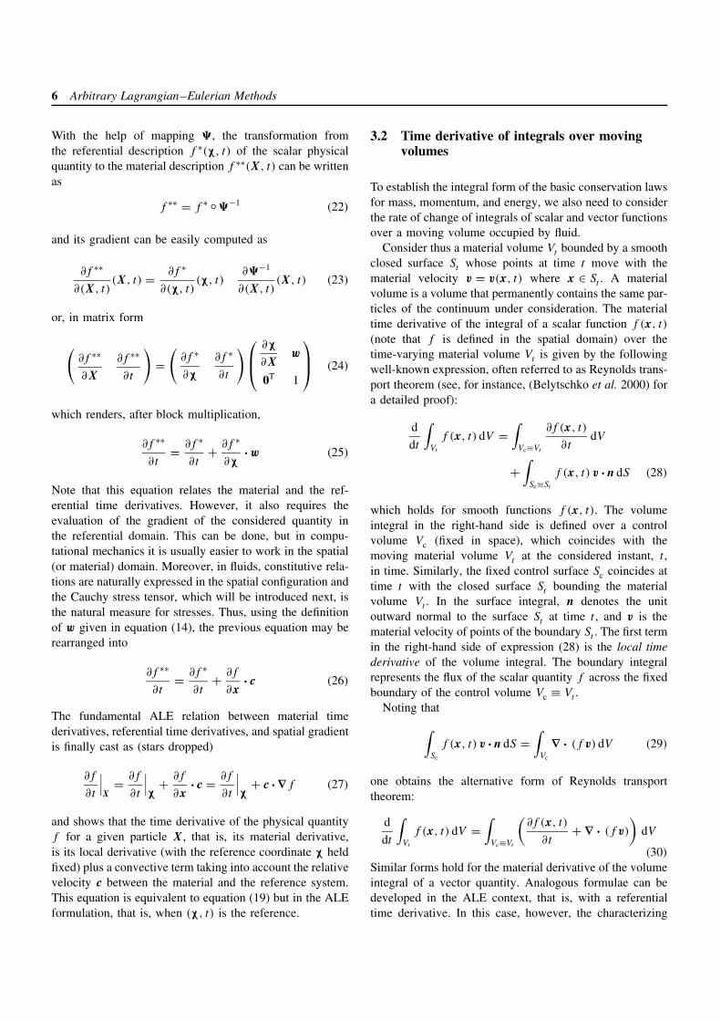
With the help of mapping �, the transformation fromthe referential description f ∗(χ, t) of the scalar physicalquantity to the material description f ∗∗(X, t) can be writtenas
f ∗∗ = f ∗ ◦�−1 (22)
and its gradient can be easily computed as
∂f ∗∗
∂(X, t)(X, t) = ∂f ∗
∂(χ, t)(χ, t)
∂�−1
∂(X, t)(X, t) (23)
or, in matrix form
(∂f ∗∗
∂X
∂f ∗∗
∂t
)=
(∂f ∗
∂χ
∂f ∗
∂t
) ∂χ
∂Xw
0T 1
(24)
which renders, after block multiplication,
∂f ∗∗
∂t= ∂f ∗
∂t+ ∂f ∗
∂χ· w (25)
Note that this equation relates the material and the ref-erential time derivatives. However, it also requires theevaluation of the gradient of the considered quantity inthe referential domain. This can be done, but in compu-tational mechanics it is usually easier to work in the spatial(or material) domain. Moreover, in fluids, constitutive rela-tions are naturally expressed in the spatial configuration andthe Cauchy stress tensor, which will be introduced next, isthe natural measure for stresses. Thus, using the definitionof w given in equation (14), the previous equation may berearranged into
∂f ∗∗
∂t= ∂f ∗
∂t+ ∂f
∂x· c (26)
The fundamental ALE relation between material timederivatives, referential time derivatives, and spatial gradientis finally cast as (stars dropped)
∂f
∂t
∣∣∣X
= ∂f
∂t
∣∣∣χ
+ ∂f
∂x· c = ∂f
∂t
∣∣∣χ
+ c ·∇f (27)
and shows that the time derivative of the physical quantityf for a given particle X, that is, its material derivative,is its local derivative (with the reference coordinate χ heldfixed) plus a convective term taking into account the relativevelocity c between the material and the reference system.This equation is equivalent to equation (19) but in the ALEformulation, that is, when (χ, t) is the reference.
3.2 Time derivative of integrals over movingvolumes
To establish the integral form of the basic conservation lawsfor mass, momentum, and energy, we also need to considerthe rate of change of integrals of scalar and vector functionsover a moving volume occupied by fluid.
Consider thus a material volume Vt bounded by a smoothclosed surface St whose points at time t move with thematerial velocity v = v(x, t) where x ∈ St . A materialvolume is a volume that permanently contains the same par-ticles of the continuum under consideration. The materialtime derivative of the integral of a scalar function f (x, t)
(note that f is defined in the spatial domain) over thetime-varying material volume Vt is given by the followingwell-known expression, often referred to as Reynolds trans-port theorem (see, for instance, (Belytschko et al. 2000) fora detailed proof):
d
dt
∫Vt
f (x, t) dV =∫
Vc≡Vt
∂f (x, t)
∂tdV
+∫
Sc≡St
f (x, t) v ·n dS (28)
which holds for smooth functions f (x, t). The volumeintegral in the right-hand side is defined over a controlvolume Vc (fixed in space), which coincides with themoving material volume Vt at the considered instant, t ,in time. Similarly, the fixed control surface Sc coincides attime t with the closed surface St bounding the materialvolume Vt . In the surface integral, n denotes the unitoutward normal to the surface St at time t , and v is thematerial velocity of points of the boundary St . The first termin the right-hand side of expression (28) is the local timederivative of the volume integral. The boundary integralrepresents the flux of the scalar quantity f across the fixedboundary of the control volume Vc ≡ Vt .
Noting that∫Sc
f (x, t) v · n dS =∫
Vc
∇ · (f v) dV (29)
one obtains the alternative form of Reynolds transporttheorem:
d
dt
∫Vt
f (x, t) dV =∫
Vc≡Vt
(∂f (x, t)
∂t+ ∇ · (f v)
)dV
(30)
Similar forms hold for the material derivative of the volumeintegral of a vector quantity. Analogous formulae can bedeveloped in the ALE context, that is, with a referentialtime derivative. In this case, however, the characterizing
Arbitrary Lagrangian–Eulerian Methods 7
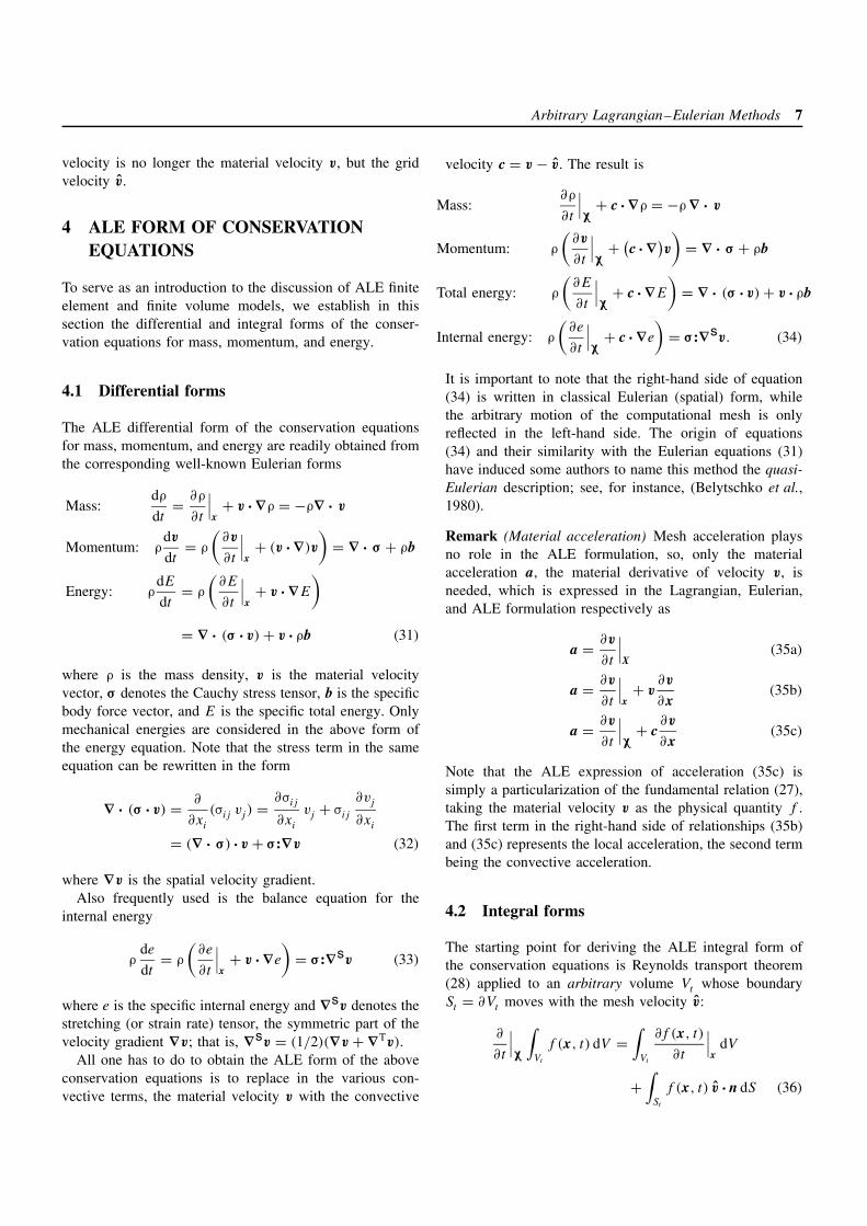
velocity is no longer the material velocity v, but the gridvelocity v.
4 ALE FORM OF CONSERVATIONEQUATIONS
To serve as an introduction to the discussion of ALE finiteelement and finite volume models, we establish in thissection the differential and integral forms of the conser-vation equations for mass, momentum, and energy.
4.1 Differential forms
The ALE differential form of the conservation equationsfor mass, momentum, and energy are readily obtained fromthe corresponding well-known Eulerian forms
Mass:dρ
dt= ∂ρ
∂t
∣∣∣x
+ v · ∇ρ = −ρ∇ · v
Momentum: ρdv
dt= ρ
(∂v
∂t
∣∣∣x
+ (v ·∇)v
)= ∇ · σ + ρb
Energy: ρdE
dt= ρ
(∂E
∂t
∣∣∣x
+ v · ∇E
)= ∇ · (σ · v) + v · ρb (31)
where ρ is the mass density, v is the material velocityvector, σ denotes the Cauchy stress tensor, b is the specificbody force vector, and E is the specific total energy. Onlymechanical energies are considered in the above form ofthe energy equation. Note that the stress term in the sameequation can be rewritten in the form
∇ · (σ · v) = ∂
∂xi
(σij vj ) = ∂σij
∂xi
vj + σij
∂vj
∂xi
= (∇ · σ) · v + σ:∇v (32)
where ∇v is the spatial velocity gradient.Also frequently used is the balance equation for the
internal energy
ρde
dt= ρ
(∂e
∂t
∣∣∣x
+ v · ∇e
)= σ:∇sv (33)
where e is the specific internal energy and ∇sv denotes thestretching (or strain rate) tensor, the symmetric part of thevelocity gradient ∇v; that is, ∇sv = (1/2)(∇v + ∇Tv).
All one has to do to obtain the ALE form of the aboveconservation equations is to replace in the various con-vective terms, the material velocity v with the convective
velocity c = v − v. The result is
Mass:∂ρ
∂t
∣∣∣χ
+ c ·∇ρ = −ρ∇ · v
Momentum: ρ
(∂v
∂t
∣∣∣χ
+ (c · ∇)
v
)= ∇ · σ + ρb
Total energy: ρ
(∂E
∂t
∣∣∣χ
+ c · ∇E
)= ∇ · (σ · v) + v · ρb
Internal energy: ρ
(∂e
∂t
∣∣∣χ
+ c · ∇e
)= σ:∇sv. (34)
It is important to note that the right-hand side of equation(34) is written in classical Eulerian (spatial) form, whilethe arbitrary motion of the computational mesh is onlyreflected in the left-hand side. The origin of equations(34) and their similarity with the Eulerian equations (31)have induced some authors to name this method the quasi-Eulerian description; see, for instance, (Belytschko et al.,1980).
Remark (Material acceleration) Mesh acceleration playsno role in the ALE formulation, so, only the materialacceleration a, the material derivative of velocity v, isneeded, which is expressed in the Lagrangian, Eulerian,and ALE formulation respectively as
a = ∂v
∂t
∣∣∣X
(35a)
a = ∂v
∂t
∣∣∣x
+ v∂v
∂x(35b)
a = ∂v
∂t
∣∣∣χ
+ c∂v
∂x(35c)
Note that the ALE expression of acceleration (35c) issimply a particularization of the fundamental relation (27),taking the material velocity v as the physical quantity f .The first term in the right-hand side of relationships (35b)and (35c) represents the local acceleration, the second termbeing the convective acceleration.
4.2 Integral forms
The starting point for deriving the ALE integral form ofthe conservation equations is Reynolds transport theorem(28) applied to an arbitrary volume Vt whose boundarySt = ∂Vt moves with the mesh velocity v:
∂
∂t
∣∣∣χ
∫Vt
f (x, t) dV =∫
Vt
∂f (x, t)
∂t
∣∣∣x
dV
+∫
St
f (x, t) v ·n dS (36)
8 Arbitrary Lagrangian–Eulerian Methods
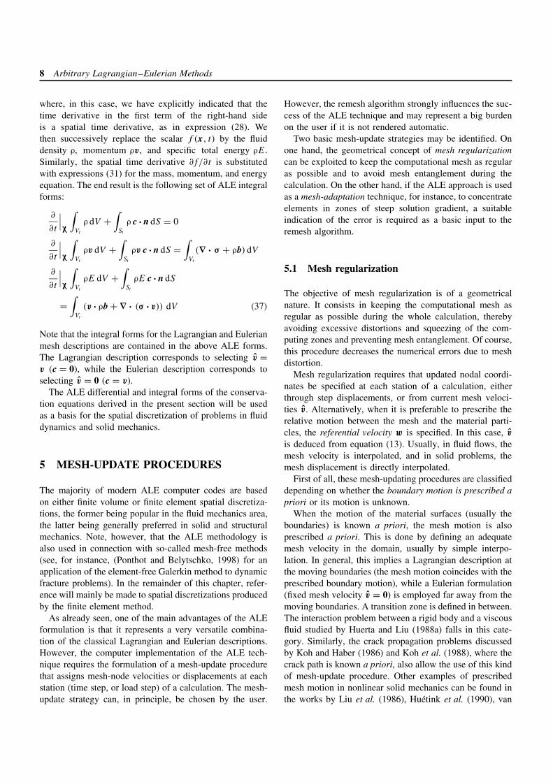
where, in this case, we have explicitly indicated that thetime derivative in the first term of the right-hand sideis a spatial time derivative, as in expression (28). Wethen successively replace the scalar f (x, t) by the fluiddensity ρ, momentum ρv, and specific total energy ρE.Similarly, the spatial time derivative ∂f/∂t is substitutedwith expressions (31) for the mass, momentum, and energyequation. The end result is the following set of ALE integralforms:
∂
∂t
∣∣∣χ
∫Vt
ρ dV +∫
St
ρ c · n dS = 0
∂
∂t
∣∣∣χ
∫Vt
ρv dV +∫
St
ρv c · n dS =∫
Vt
(∇ · σ + ρb) dV
∂
∂t
∣∣∣χ
∫Vt
ρE dV +∫
St
ρE c · n dS
=∫
Vt
(v · ρb + ∇ · (σ · v)) dV (37)
Note that the integral forms for the Lagrangian and Eulerianmesh descriptions are contained in the above ALE forms.The Lagrangian description corresponds to selecting v =v (c = 0), while the Eulerian description corresponds toselecting v = 0 (c = v).
The ALE differential and integral forms of the conserva-tion equations derived in the present section will be usedas a basis for the spatial discretization of problems in fluiddynamics and solid mechanics.
5 MESH-UPDATE PROCEDURES
The majority of modern ALE computer codes are basedon either finite volume or finite element spatial discretiza-tions, the former being popular in the fluid mechanics area,the latter being generally preferred in solid and structuralmechanics. Note, however, that the ALE methodology isalso used in connection with so-called mesh-free methods(see, for instance, (Ponthot and Belytschko, 1998) for anapplication of the element-free Galerkin method to dynamicfracture problems). In the remainder of this chapter, refer-ence will mainly be made to spatial discretizations producedby the finite element method.
As already seen, one of the main advantages of the ALEformulation is that it represents a very versatile combina-tion of the classical Lagrangian and Eulerian descriptions.However, the computer implementation of the ALE tech-nique requires the formulation of a mesh-update procedurethat assigns mesh-node velocities or displacements at eachstation (time step, or load step) of a calculation. The mesh-update strategy can, in principle, be chosen by the user.
However, the remesh algorithm strongly influences the suc-cess of the ALE technique and may represent a big burdenon the user if it is not rendered automatic.
Two basic mesh-update strategies may be identified. Onone hand, the geometrical concept of mesh regularizationcan be exploited to keep the computational mesh as regularas possible and to avoid mesh entanglement during thecalculation. On the other hand, if the ALE approach is usedas a mesh-adaptation technique, for instance, to concentrateelements in zones of steep solution gradient, a suitableindication of the error is required as a basic input to theremesh algorithm.
5.1 Mesh regularization
The objective of mesh regularization is of a geometricalnature. It consists in keeping the computational mesh asregular as possible during the whole calculation, therebyavoiding excessive distortions and squeezing of the com-puting zones and preventing mesh entanglement. Of course,this procedure decreases the numerical errors due to meshdistortion.
Mesh regularization requires that updated nodal coordi-nates be specified at each station of a calculation, eitherthrough step displacements, or from current mesh veloci-ties v. Alternatively, when it is preferable to prescribe therelative motion between the mesh and the material parti-cles, the referential velocity w is specified. In this case, v
is deduced from equation (13). Usually, in fluid flows, themesh velocity is interpolated, and in solid problems, themesh displacement is directly interpolated.
First of all, these mesh-updating procedures are classifieddepending on whether the boundary motion is prescribed apriori or its motion is unknown.
When the motion of the material surfaces (usually theboundaries) is known a priori, the mesh motion is alsoprescribed a priori. This is done by defining an adequatemesh velocity in the domain, usually by simple interpo-lation. In general, this implies a Lagrangian description atthe moving boundaries (the mesh motion coincides with theprescribed boundary motion), while a Eulerian formulation(fixed mesh velocity v = 0) is employed far away from themoving boundaries. A transition zone is defined in between.The interaction problem between a rigid body and a viscousfluid studied by Huerta and Liu (1988a) falls in this cate-gory. Similarly, the crack propagation problems discussedby Koh and Haber (1986) and Koh et al. (1988), where thecrack path is known a priori, also allow the use of this kindof mesh-update procedure. Other examples of prescribedmesh motion in nonlinear solid mechanics can be found inthe works by Liu et al. (1986), Huetink et al. (1990), van
Arbitrary Lagrangian–Eulerian Methods 9
Haaren et al. (2000), and Rodrıguez-Ferran et al. (2002),among others.
In all other cases, at least a part of the boundary is a mate-rial surface whose position must be tracked at each timestep. Thus, a Lagrangian description is prescribed along thissurface (or at least along its normal). In the first applicationsto fluid dynamics (usually free surface flows), ALE degreesof freedom were simply divided into purely Lagrangian(v = v) or purely Eulerian (v = 0). Of course, the distor-tion was thus concentrated in a layer of elements. This is,for instance, the case for numerical simulations reportedby Noh (1964), Franck and Lazarus (1964), Hirt et al.(1974), and Pracht (1975). Nodes located on moving bound-aries were Lagrangian, while internal nodes were Eulerian.This approach was used later for fluid–structure interactionproblems by Liu and Chang (1984) and in solid mechan-ics by Haber (1984) and Haber and Hariandja (1985). Thisprocedure was generalized by Hughes et al. (1981) usingthe so-called Lagrange–Euler matrix method. The referen-tial velocity, w, is defined relative to the particle velocity,v, and the mesh velocity is determined from equation (13).Huerta and Liu (1988b) improved this method avoiding theneed to solve any equation for the mesh velocity inside thedomain and ensuring an accurate tracking of the materialsurfaces by solving w · n = 0, where n is the unit outwardnormal, only along the material surfaces. Once the bound-aries are known, mesh displacements or velocities insidethe computational domain can in fact be prescribed throughpotential-type equations or interpolations as is discussednext.
In fluid–structure interaction problems, solid nodes areusually treated as Lagrangian, while fluid nodes are treatedas described above (fixed or updated according to somesimple interpolation scheme). Interface nodes between thesolid and the fluid must generally be treated as describedin Section 6.1.2. Occasionally they can be treated asLagrangian (see, for instance, (Belytschko and Kennedy,1978; Belytschko et al., 1980, 1982; Belytschko and Liu,1985); Argyris et al., 1985; Huerta and Liu, 1988b).
Once the boundary motion is known, several interpola-tion techniques are available to determine the mesh rezon-ing in the interior of the domain.
5.1.1 Transfinite mapping method
This method was originally designed for creating a mesh ona geometric region with specified boundaries; see e.g. (Gor-don and Hall, 1973; Haber and Abel, 1982; and Eriksson,1985). The general transfinite method describes an approx-imate surface or volume at a nondenumerable number ofpoints. It is this property that gives rise to the term trans-finite mapping. In the 2-D case, the transfinite mapping
can be made to exactly model all domain boundaries, and,thus, no geometric error is introduced by the mapping. Itinduces a very low-cost procedure, since new nodal coordi-nates can be obtained explicitly once the boundaries of thecomputational domain have been discretized. The main dis-advantage of this methodology is that it imposes restrictionson the mesh topology, as two opposite curves have to bediscretized with the same number of elements. It has beenwidely used by the ALE community to update nodal coor-dinates; see e.g. (Ponthot and Hogge, 1991; Yamada andKikuchi, 1993; Gadala and Wang, 1998, 1999; and Gadalaet al., 2002).
5.1.2 Laplacian smoothing and variational methods
As in mesh generation or smoothing techniques, the rezon-ing of the mesh nodes consists in solving a Laplace (orPoisson) equation for each component of the node veloc-ity or position, so that on a logically regular region themesh forms lines of equal potential. This method is alsosometimes called elliptic mesh generation and was origi-nally proposed by Winslow (1963). This technique has animportant drawback: in a nonconvex domain, nodes mayrun outside it. Techniques to preclude this pitfall eitherincrease the computational cost enormously or introducenew terms in the formulation, which are particular to eachgeometry. Examples based on this type of mesh-updatealgorithms are presented, among others, by Benson (Ben-son, 1989; Benson, 1992a; Benson, 1992b), (Liu et al.,1988, 1991), Ghosh and Kikuchi (1991), Chenot and Bel-let (1995), and Lohner and Yang (1996). An equivalentapproach based on a mechanical interpretation: (non)linearelasticity problem is used by Schreurs et al. (1986), LeTallec and Martin (1996), Belytschko et al. (2000), andArmero and Love (2003), while Cescutti et al. (1988) min-imize a functional quantifying the mesh distortion.
5.1.3 Mesh-smoothing and simple interpolations
In fact, in ALE, it is possible to use any mesh-smoothingalgorithm designed to improve the shape of the elementsonce the topology is fixed. Simple iterative averaging proce-dures can be implemented where possible; see, for instance,(Donea et al., 1982; Batina, 1991; Trepanier et al., 1993;Ghosh and Raju, 1996; and Aymone et al., 2001). A morerobust algorithm (especially in the neighborhood of bound-aries with large curvature) was proposed by Giuliani (1982)on the basis of geometric considerations. The goal of thismethod is to minimize both the squeeze and distortion ofeach element in the mesh. Donea (1983) and Huerta andCasadei (1994) show examples using this algorithm; Sar-rate and Huerta (2001) and Hermansson and Hansbo (2003)
10 Arbitrary Lagrangian–Eulerian Methods
(a) (b) (c)
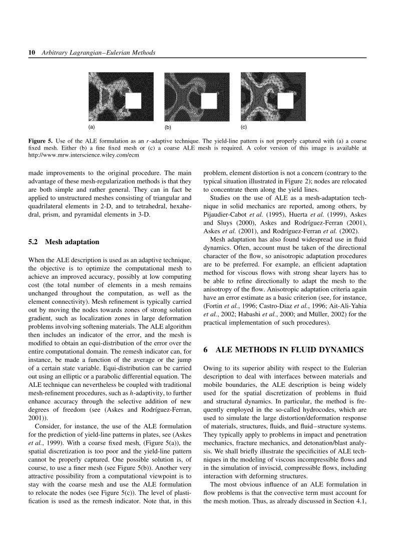
Figure 5. Use of the ALE formulation as an r-adaptive technique. The yield-line pattern is not properly captured with (a) a coarsefixed mesh. Either (b) a fine fixed mesh or (c) a coarse ALE mesh is required. A color version of this image is available athttp://www.mrw.interscience.wiley.com/ecm
made improvements to the original procedure. The mainadvantage of these mesh-regularization methods is that theyare both simple and rather general. They can in fact beapplied to unstructured meshes consisting of triangular andquadrilateral elements in 2-D, and to tetrahedral, hexahe-dral, prism, and pyramidal elements in 3-D.
5.2 Mesh adaptation
When the ALE description is used as an adaptive technique,the objective is to optimize the computational mesh toachieve an improved accuracy, possibly at low computingcost (the total number of elements in a mesh remainsunchanged throughout the computation, as well as theelement connectivity). Mesh refinement is typically carriedout by moving the nodes towards zones of strong solutiongradient, such as localization zones in large deformationproblems involving softening materials. The ALE algorithmthen includes an indicator of the error, and the mesh ismodified to obtain an equi-distribution of the error over theentire computational domain. The remesh indicator can, forinstance, be made a function of the average or the jumpof a certain state variable. Equi-distribution can be carriedout using an elliptic or a parabolic differential equation. TheALE technique can nevertheless be coupled with traditionalmesh-refinement procedures, such as h-adaptivity, to furtherenhance accuracy through the selective addition of newdegrees of freedom (see (Askes and Rodrıguez-Ferran,2001)).
Consider, for instance, the use of the ALE formulationfor the prediction of yield-line patterns in plates, see (Askeset al., 1999). With a coarse fixed mesh, (Figure 5(a)), thespatial discretization is too poor and the yield-line patterncannot be properly captured. One possible solution is, ofcourse, to use a finer mesh (see Figure 5(b)). Another veryattractive possibility from a computational viewpoint is tostay with the coarse mesh and use the ALE formulationto relocate the nodes (see Figure 5(c)). The level of plasti-fication is used as the remesh indicator. Note that, in this
problem, element distortion is not a concern (contrary to thetypical situation illustrated in Figure 2); nodes are relocatedto concentrate them along the yield lines.
Studies on the use of ALE as a mesh-adaptation tech-nique in solid mechanics are reported, among others, byPijaudier-Cabot et al. (1995), Huerta et al. (1999), Askesand Sluys (2000), Askes and Rodrıguez-Ferran (2001),Askes et al. (2001), and Rodrıguez-Ferran et al. (2002).
Mesh adaptation has also found widespread use in fluiddynamics. Often, account must be taken of the directionalcharacter of the flow, so anisotropic adaptation proceduresare to be preferred. For example, an efficient adaptationmethod for viscous flows with strong shear layers has tobe able to refine directionally to adapt the mesh to theanisotropy of the flow. Anisotropic adaptation criteria againhave an error estimate as a basic criterion (see, for instance,(Fortin et al., 1996; Castro-Diaz et al., 1996; Ait-Ali-Yahiaet al., 2002; Habashi et al., 2000; and Muller, 2002) for thepractical implementation of such procedures).
6 ALE METHODS IN FLUID DYNAMICS
Owing to its superior ability with respect to the Euleriandescription to deal with interfaces between materials andmobile boundaries, the ALE description is being widelyused for the spatial discretization of problems in fluidand structural dynamics. In particular, the method is fre-quently employed in the so-called hydrocodes, which areused to simulate the large distortion/deformation responseof materials, structures, fluids, and fluid–structure systems.They typically apply to problems in impact and penetrationmechanics, fracture mechanics, and detonation/blast analy-sis. We shall briefly illustrate the specificities of ALE tech-niques in the modeling of viscous incompressible flows andin the simulation of inviscid, compressible flows, includinginteraction with deforming structures.
The most obvious influence of an ALE formulation inflow problems is that the convective term must account forthe mesh motion. Thus, as already discussed in Section 4.1,
Arbitrary Lagrangian–Eulerian Methods 11
the convective velocity c replaces the material velocity v,which appears in the convective term of Eulerian formula-tions (see equations 31 and 34). Note that the mesh motionmay increase or decrease the convection effects. Obvi-ously, in pure convection (for instance, if a fractional-stepalgorithm is employed) or when convection is dominant,stabilization techniques must be implemented. The inter-ested reader is urged to consult Chapter 2 of Volume 3for a thorough exposition of stabilization techniques avail-able to remedy the lack of stability of the standard Galerkinformulation in convection-dominated situations, or the text-book by Donea and Huerta (2003).
It is important to note that in standard fluid dynamics, thestress tensor only depends on the pressure and (for viscousflows) on the velocity field at the point and instant underconsideration. This is not the case in solid mechanics, asdiscussed below in Section 7. Thus, stress update is not amajor concern in ALE fluid dynamics.
6.1 Boundary conditions
The rest of the discussion of the specificities of the ALE for-mulation in fluid dynamics concerns boundary conditions.In fact, boundary conditions are related to the problem, notto the description employed. Thus, the same boundary con-ditions employed in Eulerian or Lagrangian descriptionsare implemented in the ALE formulation, that is, along theboundary of the domain, kinematical and dynamical condi-tions must be defined. Usually, this is formalized as{
v = vD on �Dn ·σ = t on �N
where vD and t are the prescribed boundary velocities andtractions respectively; n is the outward unit normal to �N,and �D and �N are the two distinct subsets (Dirichlet andNeumann respectively), which define the piecewise smoothboundary of the computational domain. As usual, stressconditions on the boundaries represent the ‘natural bound-ary conditions’, and thus, they are automatically includedin the weak form of the momentum conservation equation(see 34).
If part of the boundary is composed of a material surfacewhose position is unknown, then a mixture of both condi-tions is required. The ALE formulation allows an accuratetreatment of material surfaces. The conditions required ona material surface are: (a) no particles can cross it, and(b) stresses must be continuous across the surface (if a netforce is applied to a surface of zero mass, the accelerationis infinite). Two types of material surfaces are discussedhere: free surfaces and fluid–structure interfaces, which
may or may not be frictionless (whether or not the fluidis inviscid).
6.1.1 Free surfaces
The unknown position of free surfaces can be computedusing two different approaches. First, for the simple caseof a single-valued function z = z(x, y, t), a hyperbolicequation must be solved,
∂z
∂t+ (v · ∇)z = 0
This is the kinematic equation of the surface and has beenused, for instance, by Ramaswamy and Kawahara (1987),Huerta and Liu, 1988b, 1990; Souli and Zolesio (2001).Second, a more general approach can be obtained by sim-ply imposing the obvious condition that no particle cancross the free surface (because it is a material surface).This can be imposed in a straightforward manner by usinga Lagrangian description (i.e. w = 0 or v = v) along thissurface. However, this condition may be relaxed by impos-ing only the necessary condition: w equal to zero alongthe normal to the boundary (i.e. n ·w = 0, where n is theoutward unit normal to the fluid domain, or n · v = n · v).The mesh position, normal to the free surface, is deter-mined from the normal component of the particle velocityand remeshing can be performed along the tangent; see, forinstance (Huerta and Liu, 1989) or (Braess and Wriggers,2000). In any case, these two alternatives correspond to thekinematical condition; the dynamic condition expresses thestress-free situation, n · σ = 0, and since it is a homoge-neous natural boundary condition, as mentioned earlier, itis directly taken into account by the weak formulation.
6.1.2 Fluid–structure interaction
Along solid-wall boundaries, the particle velocity is cou-pled to the rigid or flexible structure. The enforcement ofthe kinematic requirement that no particles can cross theinterface is similar to the free-surface case. Thus, conditionsn · w = 0 or n · v = n · v are also used. However, due to thecoupling between fluid and structure, extra conditions areneeded to ensure that the fluid and structural domains willnot detach or overlap during the motion. These couplingconditions depend on the fluid.
For an inviscid fluid (no shear effects), only normalcomponents are coupled because an inviscid fluid is freeto slip along the structural interface; that is,{
n · u = n · uS continuity of normal displacementsn · v = n · vS continuity of normal velocities
12 Arbitrary Lagrangian–Eulerian Methods
where the displacement/velocity of the fluid (u/v) alongthe normal to the interface must be equal to the dis-placement/velocity of the structure (uS/vS) along the samedirection. Both equations are equivalent and one or the otheris used, depending on the formulation employed (displace-ments or velocities).
For a viscous fluid, the coupling between fluid andstructure requires that velocities (or displacements) coincidealong the interface; that is,{
u = uS continuity of displacementsv = vS continuity of velocities
In practice, two nodes are placed at each point of theinterface: one fluid node and one structural node. Since thefluid is treated in the ALE formulation, the movement of thefluid mesh may be chosen completely independent of themovement of the fluid itself. In particular, we may constrainthe fluid nodes to remain contiguous to the structural nodes,so that all nodes on the sliding interface remain permanentlyaligned. This is achieved by prescribing the grid velocityv of the fluid nodes at the interface to be equal to thematerial velocity vS of the adjacent structural nodes. Thepermanent alignment of nodes at ALE interfaces greatlyfacilitates the flow of information between the fluid andstructural domains and permits fluid–structure coupling tobe effected in the simplest and the most elegant manner;that is, the imposition of the previous kinematic conditionsis simple because of the node alignment.
The dynamic condition is automatically verified alongfixed rigid boundaries, but it presents the classical difficul-ties in fluid–structure interaction problems when compat-ibility at nodal level in velocities and stresses is required(both for flexible or rigid structures whose motion is cou-pled to the fluid flow). This condition requires that thestresses in the fluid be equal to the stresses in the structure.When the behavior of the fluid is governed by the linearStokes law (σ = −p I + 2ν∇sv) or for inviscid fluids thiscondition is
−p n + 2ν(n ·∇s)v = n ·σS or − p n = n · σS
respectively, where σS is the stress tensor acting on thestructure. In the finite element representation, the continu-ous interface is replaced with a discrete approximation andinstead of a distributed interaction pressure, considerationis given to its resultant at each interface node.
There is a large amount of literature on ALE fluid–struc-ture interaction, both for flexible structures and for rigidsolids; see, among others, (Liu and Chang, 1985; Liu andGvildys, 1986; Nomura and Hughes, 1992; Le Tallec andMouro, 2001; Casadei et al., 2001; Sarrate et al., 2001; andZhang and Hisada, 2001).
Remark (Fluid–rigid-body interaction) In some circum-stances, especially when the structure is embedded in afluid and its deformations are small compared with thedisplacements and rotations of its center of gravity, it isjustified to idealize the structure as a rigid body restingon a system consisting of springs and dashpots. Typi-cal situations in which such an idealization is legitimateinclude the simulation of wind-induced vibrations in high-rise buildings or large bridge girders, the cyclic response ofoffshore structures exposed to sea currents, as well as thebehavior of structures in aeronautical and naval engineer-ing where structural loading and response are dominated byfluid-induced vibrations. An illustrative example of ALEfluid–rigid-body interaction is shown is Section 6.2.
Remark (Normal to a discrete interface) In practice, espe-cially in complex 3-D configurations, one major difficultyis to determine the normal vector at each node of thefluid–structure interface. Various algorithms have beendeveloped to deal with this issue; Casadei and Halleux(1995) and Casadei and Sala (1999) present detailed solu-tions. In 2-D, the tangent to the interface at a given node isusually defined as parallel to the line connecting the nodesat the ends of the interface segments meeting at that node.
Remark (Free surface and structure interaction) Theabove discussion of the coupling problem only applies tothose portions of the structure that are always submergedduring the calculation. As a matter of fact, there may existportions of the structure, which only come into contact withthe fluid some time after the calculation begins. This is,for instance, the case for structural parts above a fluid-freesurface. For such portions of the structural domain, somesort of sliding treatment is necessary, as for Lagrangianmethods.
6.1.3 Geometric conservation laws
In a series of papers, see (Lesoinne and Farhat, 1996;Koobus and Farhat, 1999; Guillard and Farhat, 2000; andFarhat et al., 2001), Farhat and coworkers have discussedthe notion of geometric conservation laws for unsteady flowcomputations on moving and deforming finite element orfinite volume grids.
The basic requirement is that any ALE computationalmethod should be able to predict exactly the trivial solutionof a uniform flow. The ALE equation of mass balance (37)1is usually taken as the starting point to derive the geometricconservation law. Assuming uniform fields of density ρ andmaterial velocity v, it reduces to the continuous geometricconservation law
∂
∂t
∣∣∣χ
∫Vt
dV =∫
St
v · n dS (38)
Arbitrary Lagrangian–Eulerian Methods 13
As remarked by Smith (1999), equation (38) can also bederived from the other two ALE integral conservation laws(37) with appropriate restrictions on the flow fields.
Integrating equation (38) in time from tn to tn+1 rendersthe discrete geometric conservation law (DGCL)
|�n+1e | − |�n
e | =∫ tn+1
tn
(∫St
v · n dS
)dt (39)
which states that the change in volume (or area, in 2-D)of each element from tn to tn+1 must be equal to thevolume (or area) swept by the element boundary duringthe time interval. Assuming that the volumes �e in theleft-hand side of equation (39) can be computed exactly,this amounts to requiring the exact computation of the fluxin the right-hand side also. This poses some restrictions onthe update procedure for the grid position and velocity. Forinstance, Lesoinne and Farhat (1996) show that, for first-order time-integration schemes, the mesh velocity shouldbe computed as v
n+1/2 = (xn+1 − xn)/�t . They also pointout that, although this intuitive formula was used by manytime-integrators prior to DGCLs, it is violated in someinstances, especially in fluid–structure interaction problemswhere mesh motion is coupled with structural deformation.
The practical significance of DGCLs is a debated issue inthe literature. As admitted by Guillard and Farhat (2000),‘there are recurrent assertions in the literature stating that,in practice, enforcing the DGCL when computing on mov-ing meshes is unnecessary’. Later, Farhat et al. (2001)and other authors have studied the properties of DGCL-enforcing ALE schemes from a theoretical viewpoint. Thelink between DGCLs and the stability (and accuracy)of ALE schemes is still a controversial topic of currentresearch.
6.2 Applications in ALE fluid dynamics
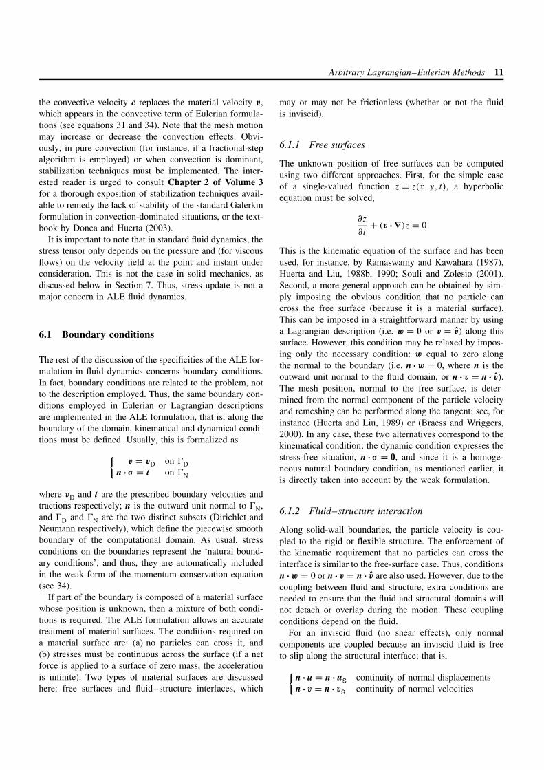
The first example consists in the computation of cross-flowand rotational oscillations of a rectangular profile. The flowis modeled by the incompressible Navier–Stokes equationsand the rectangle is regarded as rigid. The ALE formulationfor fluid–rigid-body interaction proposed by Sarrate et al.(2001) is used.
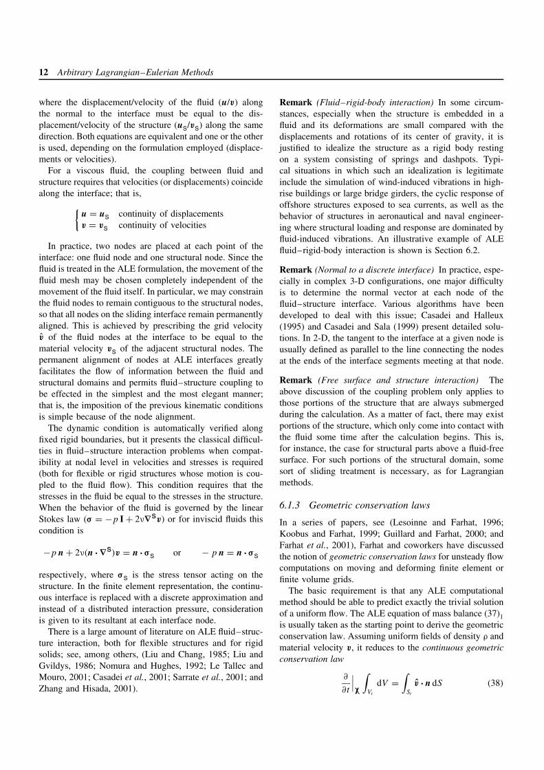
Figure 6 depicts the pressure field at two differentinstants. The flow goes from left to right. Note the cross-flow translation and the rotation of the rectangle. The ALEkinematical description avoids excessive mesh distortion(see Figure 7). For this problem, a computationally efficientrezoning strategy is obtained by dividing the mesh into threezones: (1) the mesh inside the inner circle is prescribed to
(a)
(b)
Figure 6. Flow around a rectangle. Pressure fields at two dif-ferent instants. A color version of this image is available athttp://www.mrw.interscience.wiley.com/ecm
(a)
(b)
Figure 7. Details of finite element mesh around the rectangle.The ring allows a smooth transition between the rigidly movingmesh around the rectangle and the Eulerian mesh far from it.
14 Arbitrary Lagrangian–Eulerian Methods
move rigidly attached to the rectangle (no mesh distortionand simple treatment of interface conditions); (2) the meshoutside the outer circle is Eulerian (no mesh distortion andno need to select mesh velocity); (3) a smooth transition isprescribed in the ring between the circles (mesh distortionunder control).
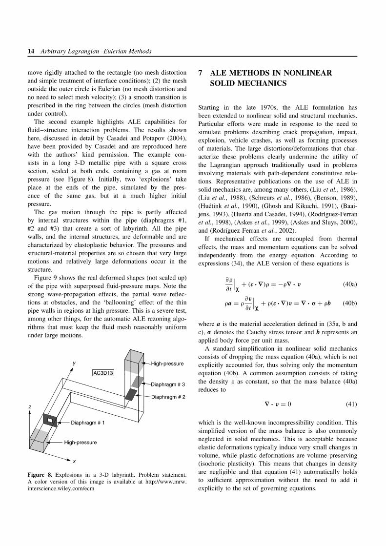
The second example highlights ALE capabilities forfluid–structure interaction problems. The results shownhere, discussed in detail by Casadei and Potapov (2004),have been provided by Casadei and are reproduced herewith the authors’ kind permission. The example con-sists in a long 3-D metallic pipe with a square crosssection, sealed at both ends, containing a gas at roompressure (see Figure 8). Initially, two ‘explosions’ takeplace at the ends of the pipe, simulated by the pres-ence of the same gas, but at a much higher initialpressure.
The gas motion through the pipe is partly affectedby internal structures within the pipe (diaphragms #1,#2 and #3) that create a sort of labyrinth. All the pipewalls, and the internal structures, are deformable and arecharacterized by elastoplastic behavior. The pressures andstructural-material properties are so chosen that very largemotions and relatively large deformations occur in thestructure.
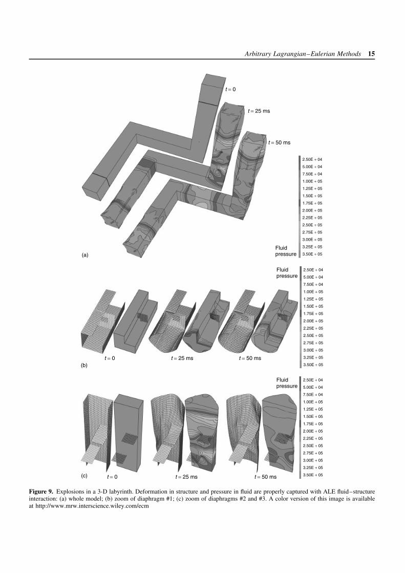
Figure 9 shows the real deformed shapes (not scaled up)of the pipe with superposed fluid-pressure maps. Note thestrong wave-propagation effects, the partial wave reflec-tions at obstacles, and the ‘ballooning’ effect of the thinpipe walls in regions at high pressure. This is a severe test,among other things, for the automatic ALE rezoning algo-rithms that must keep the fluid mesh reasonably uniformunder large motions.
x
y
z
Diaphragm # 1
Diaphragm # 2
Diaphragm # 3
High-pressure
High-pressure
AC3D13
Figure 8. Explosions in a 3-D labyrinth. Problem statement.A color version of this image is available at http://www.mrw.interscience.wiley.com/ecm
7 ALE METHODS IN NONLINEARSOLID MECHANICS
Starting in the late 1970s, the ALE formulation hasbeen extended to nonlinear solid and structural mechanics.Particular efforts were made in response to the need tosimulate problems describing crack propagation, impact,explosion, vehicle crashes, as well as forming processesof materials. The large distortions/deformations that char-acterize these problems clearly undermine the utility ofthe Lagrangian approach traditionally used in problemsinvolving materials with path-dependent constitutive rela-tions. Representative publications on the use of ALE insolid mechanics are, among many others, (Liu et al., 1986),(Liu et al., 1988), (Schreurs et al., 1986), (Benson, 1989),(Huetink et al., 1990), (Ghosh and Kikuchi, 1991), (Baai-jens, 1993), (Huerta and Casadei, 1994), (Rodrıguez-Ferranet al., 1998), (Askes et al., 1999), (Askes and Sluys, 2000),and (Rodrıguez-Ferran et al., 2002).
If mechanical effects are uncoupled from thermaleffects, the mass and momentum equations can be solvedindependently from the energy equation. According toexpressions (34), the ALE version of these equations is
∂ρ
∂t
∣∣∣χ
+ (c · ∇)ρ = −ρ∇ · v (40a)
ρa = ρ∂v
∂t
∣∣∣χ
+ ρ(c ·∇)v = ∇ · σ + ρb (40b)
where a is the material acceleration defined in (35a, b andc), σ denotes the Cauchy stress tensor and b represents anapplied body force per unit mass.
A standard simplification in nonlinear solid mechanicsconsists of dropping the mass equation (40a), which is notexplicitly accounted for, thus solving only the momentumequation (40b). A common assumption consists of takingthe density ρ as constant, so that the mass balance (40a)reduces to
∇ · v = 0 (41)
which is the well-known incompressibility condition. Thissimplified version of the mass balance is also commonlyneglected in solid mechanics. This is acceptable becauseelastic deformations typically induce very small changes involume, while plastic deformations are volume preserving(isochoric plasticity). This means that changes in densityare negligible and that equation (41) automatically holdsto sufficient approximation without the need to add itexplicitly to the set of governing equations.
Arbitrary Lagrangian–Eulerian Methods 15
t = 0
t = 25 ms
t = 50 ms
2.50E + 04
5.00E + 04
7.50E + 04
1.00E + 05
1.25E + 05
1.50E + 05
1.75E + 05
2.00E + 05
2.25E + 05
2.50E + 05
2.75E + 05
3.00E + 05
3.25E + 05
3.50E + 05Fluidpressure(a)
t = 0 t = 25 ms t = 50 ms
2.50E + 04
5.00E + 04
7.50E + 04
1.00E + 05
1.25E + 05
1.50E + 05
1.75E + 05
2.00E + 05
2.25E + 05
2.50E + 05
2.75E + 05
3.00E + 05
3.25E + 05
3.50E + 05
Fluidpressure
(b)
t = 0 t = 25 ms t = 50 ms
2.50E + 04
5.00E + 04
7.50E + 04
1.00E + 05
1.25E + 05
1.50E + 05
1.75E + 05
2.00E + 05
2.25E + 05
2.50E + 05
2.75E + 05
3.00E + 05
3.25E + 05
3.50E + 05
Fluidpressure
(c)
Figure 9. Explosions in a 3-D labyrinth. Deformation in structure and pressure in fluid are properly captured with ALE fluid–structureinteraction: (a) whole model; (b) zoom of diaphragm #1; (c) zoom of diaphragms #2 and #3. A color version of this image is availableat http://www.mrw.interscience.wiley.com/ecm
16 Arbitrary Lagrangian–Eulerian Methods
7.1 ALE treatment of steady, quasistatic anddynamic processes
In discussing the ALE form (40b) of the momentumequation, we shall distinguish between steady, quasistatic,and dynamic processes. In fact, the expression for the inertiaforces ρa critically depends on the particular type of processunder consideration.
A process is called steady if the material velocity v inevery spatial point x is constant in time. In the Euleriandescription (35b), this results in zero local acceleration∂v/∂t |x and only the convective acceleration is present inthe momentum balance, which reads
ρa = ρ(v ·∇)v = ∇ · σ + ρb (42)
In the ALE context, it is also possible to assume that aprocess is steady with respect to a grid point χ and neglectthe local acceleration ∂v/∂t |χ in the expression (35c); seefor instance, (Ghosh and Kikuchi, 1991). The momentumbalance then becomes
ρa = ρ(c · ∇)v = ∇ · σ + ρb (43)
However, the physical meaning of a null ALE localacceleration (that is, of an “ALE-steady” process) is notcompletely clear, due to the arbitrary nature of the meshvelocity and, hence, of the convective velocity c.
A process is termed quasistatic if the inertia forces ρa arenegligible with respect to the other forces in the momentumbalance. In this case, the momentum balance reduces to thestatic equilibrium equation
∇ · σ + ρb = 0 (44)
in which time and material velocity play no role. Since theinertia forces have been neglected, the different descriptionsof acceleration in equations (35a, b and c) do not appearin equation (44), which is therefore valid in both Eulerianand ALE formulations. The important conclusion is thatthere are no convective terms in the ALE momentum balancefor quasistatic processes. A process may be modeled asquasistatic if stress variations and/or body forces are muchlarger than inertia forces. This is a common situationin solid mechanics, encompassing, for instance, variousmetal-forming processes. As discussed in the next section,convective terms are nevertheless present in the ALE (andEulerian) constitutive equation for quasistatic processes.They reflect the fact that grid points are occupied bydifferent particles at different times.
Finally, in transient dynamic processes, all terms must beretained in expression (35c) for the material acceleration,
and the momentum balance equation is given by expression(40b).
7.2 ALE constitutive equations
Compared to the use of the ALE description in fluid dynam-ics, the main additional difficulty in nonlinear solid mechan-ics is the design of an appropriate stress-update procedureto deal with history-dependent constitutive equations. Asalready mentioned, constitutive equations of ALE nonlin-ear solid mechanics contain convective terms that accountfor the relative motion between mesh and material. This isthe case for both hypoelastoplastic and hyperelastoplasticmodels.
7.2.1 Constitutive equations for ALEhypoelastoplasticity
Hypoelastoplastic models are based on an additive decom-position of the stretching tensor ∇sv (symmetric part ofthe velocity gradient) into elastic and plastic parts; see, forinstance, (Belytschko et al., 2000) or (Bonet and Wood,1997). They were used in the first ALE formulations forsolid mechanics and are still the standard choice. In thesemodels, material behavior is described by a rate-form con-stitutive equation
σ� = f (σ, ∇sv) (45)
relating an objective rate of Cauchy stress σ� to stress andstretching. The material rate of stress
σ = ∂σ
∂t
∣∣∣X
= ∂σ
∂t
∣∣∣χ
+ (c ·∇)σ (46)
cannot be employed in relation (45) to measure the stressrate because it is not an objective tensor, so large rigid-body rotations are not properly treated. An objective rateof stress is obtained by adding to σ some terms that ensurethe objectivity of σ�; see, for instance, (Malvern, 1969) or(Belytschko et al., 2000). Two popular objective rates arethe Truesdell rate and the Jaumann rate
σ� = σ − ∇wv · σ − σ · (∇wv)T (47)
where ∇wv = 12 (∇v − ∇Tv) is the spin tensor.
Substitution of equation (47) (or similar expressions forother objective stress rates) into equation (45) yields
σ = q(σ, ∇sv, . . .) (48)
where q contains both f and the terms in σ�, which ensureits objectivity.
Arbitrary Lagrangian–Eulerian Methods 17
In the ALE context, referential time derivatives, notmaterial time derivatives, are employed to represent evolu-tion in time. Combining expression (46) of the material rateof stress and the constitutive relation (48) yields a rate-formconstitutive equation for ALE nonlinear solid mechanics
σ = ∂σ
∂t
∣∣∣χ
+ (c ·∇)σ = q (49)
where, again, a convective term reflects the motion ofmaterial particles relative to the mesh. Note that this relativemotion is inherent in ALE kinematics, so the convectiveterm is present in all the situations described in Section 7.1,including quasistatic processes.
Because of this convective effect, the stress update cannotbe performed as simply as in the Lagrangian formulation,in which the element Gauss points correspond to the samematerial particles during the whole calculation. In fact, theaccurate treatment of the convective terms in ALE rate-typeconstitutive equations is a key issue in the accuracy of theformulation, as discussed in Section 7.3.
7.2.2 Constitutive equations for ALEhyperelastoplasticity
Hyperelastoplastic models are based on a multiplicativedecomposition of the deformation gradient into elastic andplastic parts, F = FeFp; see, for instance, (Belytschko et al.,2000) or (Bonet and Wood, 1997). They have only veryrecently been combined with the ALE description (see(Rodrıguez-Ferran et al., 2002) and (Armero and Love,2003)).
The evolution of stresses is not described by means of arate-form equation, but in closed form as
τ = 2dW
dbe be (50)
where be = Fe · (Fe)T is the elastic left Cauchy–Greentensor, W is the free energy function, and τ = det(F)σ isthe Kirchhoff stress tensor.
Plastic flow is described by means of the flow rule
be − ∇v · be − be · (∇v)T = −2γm(τ) · be (51)
The left-hand side of equation (51) is the Lie derivative ofbe with respect to the material velocity v. In the right-handside, m is the flow direction and γ is the plastic multiplier.
Using the fundamental ALE relation (27) between mate-rial and referential time derivatives, the flow rule (51) canbe recast as
∂be
∂t
∣∣∣χ
+ (c · ∇)be = ∇v · be + be · (∇v)T − 2γm(τ) · be
(52)
Note that, like in equation (49), a convective term in thisconstitutive equation reflects the relative motion betweenmesh and material.
7.3 Stress-update procedures
In the context of hypoelastoplasticity, various strategieshave been proposed for coping with the convective termsin equation (49). Following Benson (1992b), they can beclassified into split and unsplit methods.
If an unsplit method is employed, the complete rateequation (49) is integrated forward in time, includingboth the convective term and the material term q. Thisapproach is followed, among others, by Liu et al. (1986),who employed an explicit time-stepping algorithm and byGhosh and Kikuchi (1991), who used an implicit unsplitformulation.
On the other hand, split, or fractional-step methods treatthe material and convective terms in (49) in two distinctphases: a material (or Lagrangian) phase is followed bya convection (or transport) phase. In exchange for a cer-tain loss in accuracy due to splitting, split methods aresimpler and especially suitable in upgrading a Lagrangiancode to the ALE description. An implicit split formu-lation is employed by Huetink et al. (1990) to modelmetal-forming processes. An example of explicit split for-mulation may be found in (Huerta and Casadei, 1994),where ALE finite elements are used to model fast-transientphenomena.
The situation is completely analogous for hyperelasto-plasticity, and similar comments apply to the split or unsplittreatment of material and convective effects. In fact, ifa split approach is chosen, see (Rodrıguez-Ferran et al.,2002), the only differences with respect to the hypoe-lastoplastic models are (1) the constitutive model for theLagrangian phase (hypo/hyper) and (2) the quantities to betransported in the convection phase.
7.3.1 Lagrangian phase
In the Lagrangian phase, convective effects are neglected.The constitutive equations recover their usual expressions(48) and (51) for hypo- and hyper-models respectively.The ALE kinematical description has (momentarily) dis-appeared from the formulation, so all the concepts, ideas,and algorithms of large strain solid mechanics with aLagrangian description apply (see (Bonet and Wood, 1997);(Belytschko et al., 2000) and Chapter 7 of Volume 2).
The issue of objectivity is one of the main differencesbetween hypo- and hypermodels. When devising time-integration algorithms to update stresses from σn to σn+1

18 Arbitrary Lagrangian–Eulerian Methods
in hypoelastoplastic models, a typical requirement is incre-mental objectivity (that is, the appropriate treatment ofrigid-body rotations over the time interval [tn, tn+1]). Inhyperelastoplastic models, on the contrary, objectivity isnot an issue at all, because there is no rate equation for thestress tensor.
7.3.2 Convection phase
The convective effects neglected before have to be accoun-ted for now. Since material effects have already been treatedin the Lagrangian phase, the ALE constitutive equationsread simply
∂σ
∂t
∣∣∣χ
+ (c · ∇)σ = 0; ∂be
∂t
∣∣∣χ
+ (c · ∇)be = 0;∂α
∂t
∣∣∣χ
+ (c · ∇)α = 0 (53)
Equations (53)1 and (53)2 correspond to hypo- andhyperelastoplastic models respectively (cf. with equa-tions 49 and 52). In equation (53)3, valid for both hypo-and hyper-models, α is the set of all the material-dependentvariables, i.e. variables associated with the material particleX: internal variables for hardening or softening plasticity,the volume change in nonisochoric plasticity, and so on,see (Rodrıguez-Ferran et al., 2002).
The three equations in (53) can be written more com-pactly as
∂�∂t
∣∣∣χ
+ (c · ∇)� = 0 (54)
where � represents the appropriate variable in each case.Note that equation (54) is simply a first-order linear hyper-bolic PDE, which governs the transport of field � by thevelocity field c. However, two important aspects should beconsidered in the design of numerical algorithms for thesolution of this equation:
1. � is a tensor (for σ and be) or vector-like (for α) field,so equation (54) should be solved for each component� of �:
∂�∂t
∣∣∣χ
+ c · ∇� = 0 (55)
Since the number of scalar equations (55) may be rel-atively large (for instance: eight for a 3-D computationwith a plastic model with two internal variables), theneed for efficient convection algorithms is a key issuein ALE nonlinear solid mechanics.
2. � is a Gauss-point-based (i.e. not a nodal-based)quantity, so it is discontinuous across finite elementedges. For this reason, its gradient ∇� cannot be
reliably computed at the element level. In fact, handling∇� is the main numerical challenge in ALE stressupdate.
Two different strategies may be used to tackle thedifficulties associated with ∇�. One possible approach isto approximate � by a continuous field �, and replace∇� by ∇� in equation (55). The smoothed field � canbe obtained, for instance, by least-squares approximation,see (Huetink et al., 1990).
Another possibility is to retain the discontinuous field �and devise appropriate algorithms that account for this fact.To achieve this aim, a fruitful observation is noting that,for a piecewise constant field �, equation (55) is the well-known Riemann problem. Through this connection, theALE community has exploited the expertise on approximateRiemann solvers of the CFD community, see (Le Veque,1990).
Although � is, in general, not constant for each element(expect for one-point quadratures), it can be approximatedby a piecewise constant field in a simple manner. Figure 10depicts a four-noded quadrilateral with a 2 × 2 quadraturesubdivided into four subelements. If the value of � foreach Gauss point is taken as representative for the wholesubelement, then a field constant within each subelementresults.
In this context, equation (55) can be solved explicitlyby looping all the subelements in the mesh by means ofa Godunov-like technique based on Godunov’s method forconservation laws, see (Rodrıguez-Ferran et al., 1998):
�n+1 = �L − �t
V
N�∑�=1
f�(�c� − �L)
[1 − sign(f�)
](56)
Node
Gauss point
Figure 10. Finite element subdivided into subelements for theGodunov-like stress update.
Arbitrary Lagrangian–Eulerian Methods 19
According to equation (56), the Lagrangian (i.e. after theLagrangian phase) value �L is updated into the final value�n+1 by taking into account the flux of � across thesubelement edges. In the second term on the right-hand side,�t is the time step, V is the volume (or area, in 2-D) of thesubelement, N� is the number of edges per subelement, �c
�
is the value of � in the contiguous subelement across edge�, and f� is the flux of convective velocity across edge �,f� = ∫
�(c · n) d�. Note that a full-donor (i.e. full upwind)
approach is obtained by means of sign(f�).
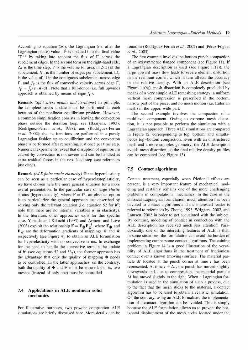
Remark (Split stress update and iterations) In principle,the complete stress update must be performed at eachiteration of the nonlinear equilibrium problem. However,a common simplification consists in leaving the convectionphase outside the iteration loop, see (Baaijens, 1993);(Rodrıguez-Ferran et al., 1998); and (Rodrıguez-Ferranet al., 2002); that is, iterations are performed in a purelyLagrangian fashion up to equilibrium and the convectionphase is performed after remeshing, just once per time step.Numerical experiments reveal that disruption of equilibriumcaused by convection is not severe and can be handled asextra residual forces in the next load step (see referencesjust cited).
Remark (ALE finite strain elasticity) Since hyperelasticitycan be seen as a particular case of hyperelastoplasticity,we have chosen here the more general situation for a moreuseful presentation. In the particular case of large elasticstrains (hyperelasticity), where F = Fe, an obvious optionis to particularize the general approach just described bysolving only the relevant equation (i.e. equation 52 for be;note that there are no internal variables α in elasticity).In the literature, other approaches exist for this specificcase. Yamada and Kikuchi (1993) and Armero and Love(2003) exploit the relationship F = F�F−1
�, where F� and
F� are the deformation gradients of mappings � and �
respectively (see Figure 4), to obtain an ALE formulationfor hyperelasticity with no convective terms. In exchangefor the need to handle the convective term in the updateof be (see equations 52 and 532), the former approach hasthe advantage that only the quality of mapping � needsto be controlled. In the latter approaches, on the contrary,both the quality of � and � must be ensured; that is, twomeshes (instead of only one) must be controlled.
7.4 Applications in ALE nonlinear solidmechanics
For illustrative purposes, two powder compaction ALEsimulations are briefly discussed here. More details can be
found in (Rodrıguez-Ferran et al., 2002) and (Perez-Foguetet al., 2003).
The first example involves the bottom punch compactionof an axisymmetric flanged component (see Figure 11). Ifa Lagrangian description is used (see Figure 11(a)), thelarge upward mass flow leads to severe element distortionin the reentrant corner, which in turn affects the accuracyin the relative density. With an ALE description (seeFigure 11(b)), mesh distortion is completely precluded bymeans of a very simple ALE remeshing strategy: a uniformvertical mesh compression is prescribed in the bottom,narrow part of the piece, and no mesh motion (i.e. Eulerianmesh) in the upper, wide part.
The second example involves the compaction of amultilevel component. Owing to extreme mesh distor-tion, it is not possible to perform the simulation with aLagrangian approach. Three ALE simulations are comparedin Figure 12, corresponding to top, bottom, and simulta-neous top–bottom compaction. Even with an unstructuredmesh and a more complex geometry, the ALE descriptionavoids mesh distortion, so the final relative density profilescan be computed (see Figure 13).
7.5 Contact algorithms
Contact treatment, especially when frictional effects arepresent, is a very important feature of mechanical mod-eling and certainly remains one of the more challengingproblems in computational mechanics. In the case of theclassical Lagrangian formulation, much attention has beendevoted to contact algorithms and the interested reader isreferred to references by Zhong, 1993, Wriggers, 2002, andLaursen, 2002 in order to get acquainted with the subject.By contrast, modeling of contact in connection with theALE description has received much less attention. Para-doxically, one of the interesting features of ALE is that,in some situations, the formulation can avoid the burden ofimplementing cumbersome contact algorithms. The coiningproblem in Figure 14 is a good illustration of the versa-tility of ALE algorithms in the treatment of frictionlesscontact over a known (moving) surface. The material par-ticle M located at the punch corner at time t has beenrepresented. At time t + �t , the punch has moved slightlydownwards and, due to compression, the material particleM has moved slightly to the right. When a Lagrangian for-mulation is used in the simulation of such a process, dueto the fact that the mesh sticks to the material, a contactalgorithm has to be used to obtain a realistic simulation.On the contrary, using an ALE formalism, the implementa-tion of a contact algorithm can be avoided. This is simplybecause the ALE formulation allows us to prevent the hor-izontal displacement of the mesh nodes located under the
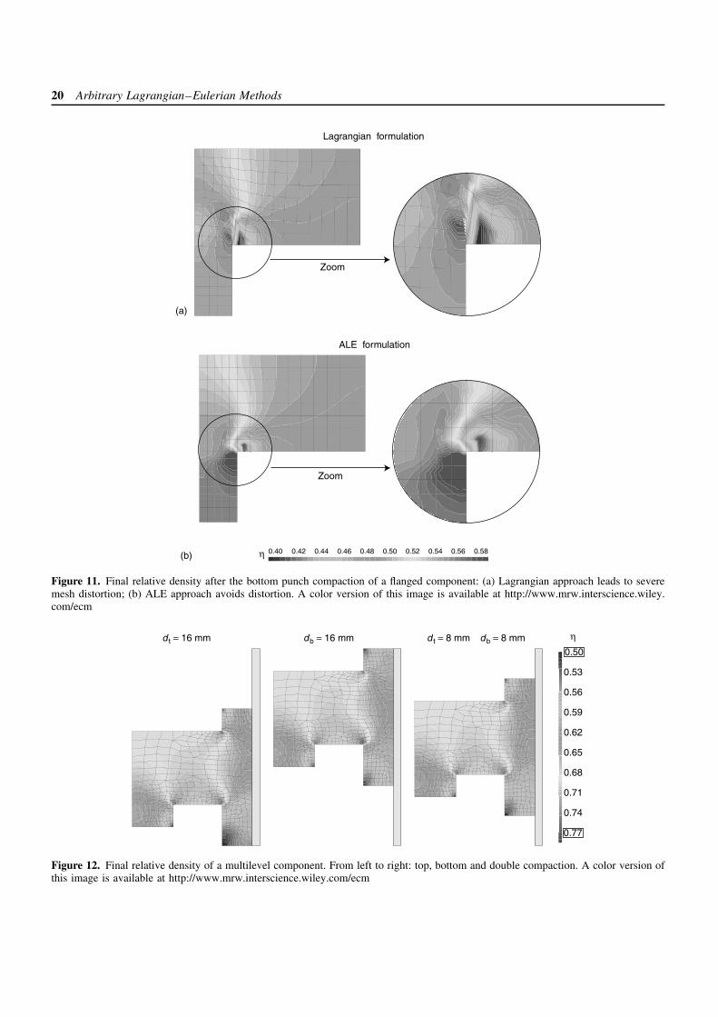
20 Arbitrary Lagrangian–Eulerian Methods
0.40 0.42 0.44 0.46 0.48 0.50 0.52 0.54 0.56 0.58η
ALE formulation
Zoom
(b)
Lagrangian formulation
Zoom
(a)
Figure 11. Final relative density after the bottom punch compaction of a flanged component: (a) Lagrangian approach leads to severemesh distortion; (b) ALE approach avoids distortion. A color version of this image is available at http://www.mrw.interscience.wiley.com/ecm
dt = 8 mm db = 8 mmdt = 16 mm db = 16 mm
0.56
0.59
0.62
0.65
0.68
0.71
0.74
0.53
η
0.77
0.50
Figure 12. Final relative density of a multilevel component. From left to right: top, bottom and double compaction. A color version ofthis image is available at http://www.mrw.interscience.wiley.com/ecm
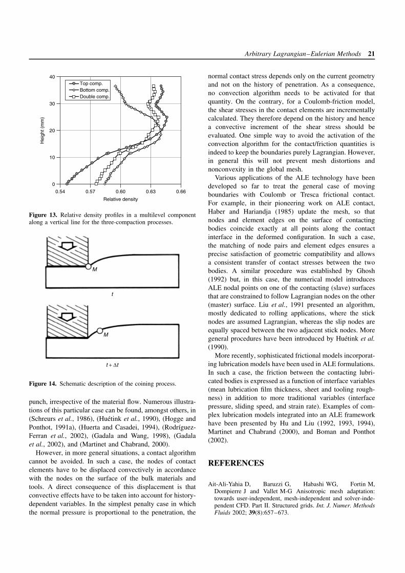
Arbitrary Lagrangian–Eulerian Methods 21
0
10
20
30
40
0.54 0.57 0.60 0.63 0.66
Relative density
Hei
ght (
mm
)
Top comp.Bottom comp.Double comp.
Figure 13. Relative density profiles in a multilevel componentalong a vertical line for the three-compaction processes.
M
t
M
t + ∆t
Figure 14. Schematic description of the coining process.
punch, irrespective of the material flow. Numerous illustra-tions of this particular case can be found, amongst others, in(Schreurs et al., 1986), (Huetink et al., 1990), (Hogge andPonthot, 1991a), (Huerta and Casadei, 1994), (Rodrıguez-Ferran et al., 2002), (Gadala and Wang, 1998), (Gadalaet al., 2002), and (Martinet and Chabrand, 2000).
However, in more general situations, a contact algorithmcannot be avoided. In such a case, the nodes of contactelements have to be displaced convectively in accordancewith the nodes on the surface of the bulk materials andtools. A direct consequence of this displacement is thatconvective effects have to be taken into account for history-dependent variables. In the simplest penalty case in whichthe normal pressure is proportional to the penetration, the
normal contact stress depends only on the current geometryand not on the history of penetration. As a consequence,no convection algorithm needs to be activated for thatquantity. On the contrary, for a Coulomb-friction model,the shear stresses in the contact elements are incrementallycalculated. They therefore depend on the history and hencea convective increment of the shear stress should beevaluated. One simple way to avoid the activation of theconvection algorithm for the contact/friction quantities isindeed to keep the boundaries purely Lagrangian. However,in general this will not prevent mesh distortions andnonconvexity in the global mesh.
Various applications of the ALE technology have beendeveloped so far to treat the general case of movingboundaries with Coulomb or Tresca frictional contact.For example, in their pioneering work on ALE contact,Haber and Hariandja (1985) update the mesh, so thatnodes and element edges on the surface of contactingbodies coincide exactly at all points along the contactinterface in the deformed configuration. In such a case,the matching of node pairs and element edges ensures aprecise satisfaction of geometric compatibility and allowsa consistent transfer of contact stresses between the twobodies. A similar procedure was established by Ghosh(1992) but, in this case, the numerical model introducesALE nodal points on one of the contacting (slave) surfacesthat are constrained to follow Lagrangian nodes on the other(master) surface. Liu et al., 1991 presented an algorithm,mostly dedicated to rolling applications, where the sticknodes are assumed Lagrangian, whereas the slip nodes areequally spaced between the two adjacent stick nodes. Moregeneral procedures have been introduced by Huetink et al.(1990).
More recently, sophisticated frictional models incorporat-ing lubrication models have been used in ALE formulations.In such a case, the friction between the contacting lubri-cated bodies is expressed as a function of interface variables(mean lubrication film thickness, sheet and tooling rough-ness) in addition to more traditional variables (interfacepressure, sliding speed, and strain rate). Examples of com-plex lubrication models integrated into an ALE frameworkhave been presented by Hu and Liu (1992, 1993, 1994),Martinet and Chabrand (2000), and Boman and Ponthot(2002).
REFERENCES
Ait-Ali-Yahia D, Baruzzi G, Habashi WG, Fortin M,Dompierre J and Vallet M-G Anisotropic mesh adaptation:towards user-independent, mesh-independent and solver-inde-pendent CFD. Part II. Structured grids. Int. J. Numer. MethodsFluids 2002; 39(8):657–673.
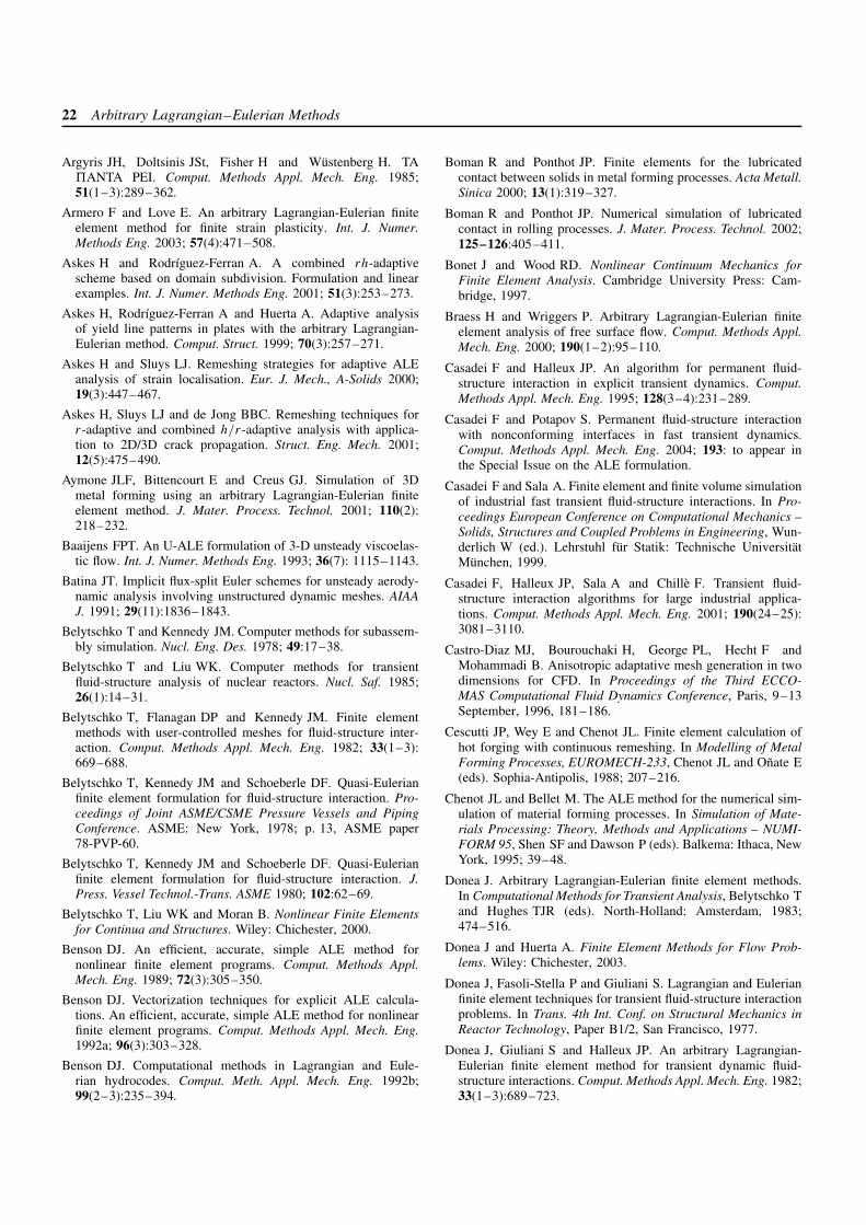
22 Arbitrary Lagrangian–Eulerian Methods
Argyris JH, Doltsinis JSt, Fisher H and Wustenberg H. TA�ANTA PEI. Comput. Methods Appl. Mech. Eng. 1985;51(1–3):289–362.
Armero F and Love E. An arbitrary Lagrangian-Eulerian finiteelement method for finite strain plasticity. Int. J. Numer.Methods Eng. 2003; 57(4):471–508.
Askes H and Rodrıguez-Ferran A. A combined rh-adaptivescheme based on domain subdivision. Formulation and linearexamples. Int. J. Numer. Methods Eng. 2001; 51(3):253–273.
Askes H, Rodrıguez-Ferran A and Huerta A. Adaptive analysisof yield line patterns in plates with the arbitrary Lagrangian-Eulerian method. Comput. Struct. 1999; 70(3):257–271.
Askes H and Sluys LJ. Remeshing strategies for adaptive ALEanalysis of strain localisation. Eur. J. Mech., A-Solids 2000;19(3):447–467.
Askes H, Sluys LJ and de Jong BBC. Remeshing techniques forr-adaptive and combined h/r-adaptive analysis with applica-tion to 2D/3D crack propagation. Struct. Eng. Mech. 2001;12(5):475–490.
Aymone JLF, Bittencourt E and Creus GJ. Simulation of 3Dmetal forming using an arbitrary Lagrangian-Eulerian finiteelement method. J. Mater. Process. Technol. 2001; 110(2):218–232.
Baaijens FPT. An U-ALE formulation of 3-D unsteady viscoelas-tic flow. Int. J. Numer. Methods Eng. 1993; 36(7): 1115–1143.
Batina JT. Implicit flux-split Euler schemes for unsteady aerody-namic analysis involving unstructured dynamic meshes. AIAAJ. 1991; 29(11):1836–1843.
Belytschko T and Kennedy JM. Computer methods for subassem-bly simulation. Nucl. Eng. Des. 1978; 49:17–38.
Belytschko T and Liu WK. Computer methods for transientfluid-structure analysis of nuclear reactors. Nucl. Saf. 1985;26(1):14–31.
Belytschko T, Flanagan DP and Kennedy JM. Finite elementmethods with user-controlled meshes for fluid-structure inter-action. Comput. Methods Appl. Mech. Eng. 1982; 33(1–3):669–688.
Belytschko T, Kennedy JM and Schoeberle DF. Quasi-Eulerianfinite element formulation for fluid-structure interaction. Pro-ceedings of Joint ASME/CSME Pressure Vessels and PipingConference. ASME: New York, 1978; p. 13, ASME paper78-PVP-60.
Belytschko T, Kennedy JM and Schoeberle DF. Quasi-Eulerianfinite element formulation for fluid-structure interaction. J.Press. Vessel Technol.-Trans. ASME 1980; 102:62–69.
Belytschko T, Liu WK and Moran B. Nonlinear Finite Elementsfor Continua and Structures. Wiley: Chichester, 2000.
Benson DJ. An efficient, accurate, simple ALE method fornonlinear finite element programs. Comput. Methods Appl.Mech. Eng. 1989; 72(3):305–350.
Benson DJ. Vectorization techniques for explicit ALE calcula-tions. An efficient, accurate, simple ALE method for nonlinearfinite element programs. Comput. Methods Appl. Mech. Eng.1992a; 96(3):303–328.
Benson DJ. Computational methods in Lagrangian and Eule-rian hydrocodes. Comput. Meth. Appl. Mech. Eng. 1992b;99(2–3):235–394.
Boman R and Ponthot JP. Finite elements for the lubricatedcontact between solids in metal forming processes. Acta Metall.Sinica 2000; 13(1):319–327.
Boman R and Ponthot JP. Numerical simulation of lubricatedcontact in rolling processes. J. Mater. Process. Technol. 2002;125–126:405–411.
Bonet J and Wood RD. Nonlinear Continuum Mechanics forFinite Element Analysis. Cambridge University Press: Cam-bridge, 1997.
Braess H and Wriggers P. Arbitrary Lagrangian-Eulerian finiteelement analysis of free surface flow. Comput. Methods Appl.Mech. Eng. 2000; 190(1–2):95–110.
Casadei F and Halleux JP. An algorithm for permanent fluid-structure interaction in explicit transient dynamics. Comput.Methods Appl. Mech. Eng. 1995; 128(3–4):231–289.
Casadei F and Potapov S. Permanent fluid-structure interactionwith nonconforming interfaces in fast transient dynamics.Comput. Methods Appl. Mech. Eng. 2004; 193: to appear inthe Special Issue on the ALE formulation.
Casadei F and Sala A. Finite element and finite volume simulationof industrial fast transient fluid-structure interactions. In Pro-ceedings European Conference on Computational Mechanics –Solids, Structures and Coupled Problems in Engineering, Wun-derlich W (ed.). Lehrstuhl fur Statik: Technische UniversitatMunchen, 1999.
Casadei F, Halleux JP, Sala A and Chille F. Transient fluid-structure interaction algorithms for large industrial applica-tions. Comput. Methods Appl. Mech. Eng. 2001; 190(24–25):3081–3110.
Castro-Diaz MJ, Bourouchaki H, George PL, Hecht F andMohammadi B. Anisotropic adaptative mesh generation in twodimensions for CFD. In Proceedings of the Third ECCO-MAS Computational Fluid Dynamics Conference, Paris, 9–13September, 1996, 181–186.
Cescutti JP, Wey E and Chenot JL. Finite element calculation ofhot forging with continuous remeshing. In Modelling of MetalForming Processes, EUROMECH-233, Chenot JL and Onate E(eds). Sophia-Antipolis, 1988; 207–216.
Chenot JL and Bellet M. The ALE method for the numerical sim-ulation of material forming processes. In Simulation of Mate-rials Processing: Theory, Methods and Applications – NUMI-FORM 95, Shen SF and Dawson P (eds). Balkema: Ithaca, NewYork, 1995; 39–48.
Donea J. Arbitrary Lagrangian-Eulerian finite element methods.In Computational Methods for Transient Analysis, Belytschko Tand Hughes TJR (eds). North-Holland: Amsterdam, 1983;474–516.
Donea J and Huerta A. Finite Element Methods for Flow Prob-lems. Wiley: Chichester, 2003.
Donea J, Fasoli-Stella P and Giuliani S. Lagrangian and Eulerianfinite element techniques for transient fluid-structure interactionproblems. In Trans. 4th Int. Conf. on Structural Mechanics inReactor Technology, Paper B1/2, San Francisco, 1977.
Donea J, Giuliani S and Halleux JP. An arbitrary Lagrangian-Eulerian finite element method for transient dynamic fluid-structure interactions. Comput. Methods Appl. Mech. Eng. 1982;33(1–3):689–723.
Arbitrary Lagrangian–Eulerian Methods 23
Eriksson LE. Practical three-dimensional mesh generation usingtransfinite interpolation. SIAM J. Sci. Statist. Comput. 1985;6(3):712–741.
Farhat C, Geuzaine Ph and Grandmont C. The discrete geometricconservation law and the nonlinear stability of ALE schemesfor the solution of flow problems on moving grids. J. Comput.Phys. 2001; 174(2):669–694.
Fortin M, Vallet M-G, Dompierre J, Bourgault Y and HabashiWG. Anisotropic mesh adaptation: theory, validation and appli-cations. In Proceedings of the Third ECCOMAS ComputationalFluid Dynamics Conference, Paris, 9–13 September, 1996,174–180.
Franck RM and Lazarus RB. Mixed Eulerian-Lagrangian method.In Methods in Computational Physics, Vol. 3: Fundamentalmethods in Hydrodynamics, Alder B, Fernbach S and Roten-berg M (eds). Academic Press: New York, 1964; 47–67.
Gadala MS and Wang J. ALE formulation and its applicationin solid mechanics. Comput. Methods Appl. Mech. Eng. 1998;167(1–2):33–55.
Gadala MS and Wang J. Simulation of metal forming processeswith finite element methods. Int. J. Numer. Methods Eng. 1999;44(10):1397–1428.
Gadala MS, Movahhedy MR and Wang J. On the mesh motionfor ALE modeling of metal forming processes. Finite Elem.Anal. Des. 2002; 38(5):435–459.
Ghosh S. Arbitrary Lagrangian-Eulerian finite element analysis oflarge deformation in contacting bodies. Int. J. Numer. MethodsEng. 1992; 33(9):1891–1925.
Ghosh S and Kikuchi N. An arbitrary Lagrangian-Eulerian finiteelement method for large deformation analysis of elastic-viscoplastic solids. Comput. Methods Appl. Mech. Eng. 1991;86(2):127–188.
Ghosh S and Raju S. R-S adapted arbitrary Lagrangian Eule-rian finite element method for metal-forming problems withstrain localization. Int. J. Numer. Methods Eng. 1996; 39(19):3247–3272.
Giuliani S. An algorithm for continuous rezoning of the hydro-dynamic grid in arbitrary Lagrangian-Eulerian computer codes.Nucl. Eng. Des. 1982; 72:205–212.
Gordon WJ and Hall CH. Construction of curvilinear co-ordinatesystems and applications to mesh generation. Int. J. Numer.Methods Eng. 1973; 7(4):461–477.
Guillard H and Farhat C. On the significance of the geo-metric conservation law for flow computations on mov-ing meshes. Comput. Methods Appl. Mech. Eng. 2000;190(11–12):1467–1482.
Habashi WG, Fortin M, Vallet M-G, Dompierre J, Bourgault Yand Ait-Ali-Yahia D. Anisotropic mesh adaptation: towardsuser-independent, mesh-independent and solver-independentCFD solutions. Part I: Theory. Int. J. Numer. Methods Fluids2000; 32(6):725–744.
Haber RB. A mixed Eulerian-Lagrangian displacement modelfor large-deformation analysis in solid mechanics. Comput.Methods Appl. Mech. Eng. 1984; 43(3):277–292.
Haber R and Abel JF. Discrete transfinite mappings for thedescription and meshing of three-dimensional surfaces using
interactive computer graphics. Int. J. Numer. Methods Eng.1982; 18(1):41–66.
Haber RB and Hariandja BH. Computational strategies for nonlin-ear and fracture mechanics problems. An Eulerian-Lagrangianfinite element approach to large deformation frictional contact.Comput. Struct. 1985; 20(1–3):193–201.
Hermansson J and Hansbo P. A variable diffusion methodfor mesh smoothing. Commun. Numer. Methods Eng. 2003;19(11):897–908.
Hirt CW, Amsden AA and Cook JL. An arbitrary Lagrangian-Eulerian computing method for all flow speeds. J. Comput.Phys. 1974; 14:227–253. Reprinted in J. Comput. Phys. 1997;135(2):203–216.
Hogge M and Ponthot JP. Metal forming analysis via Eulerian-Lagrangian FEM with adaptive mesh. Latin Am. Res. 1991;21:217–224.
Hu YK and Liu WK. ALE finite element formulation forring rolling analysis. Int. J. Numer. Methods Eng. 1992;33(6):1217–1236.
Hu YK and Liu WK. An ALE hydrodynamic lubrication finiteelement method with application to strip rolling. Int. J. Numer.Methods Eng. 1993; 36(5):855–880.
Hu YK and Liu WK. Finite element hydrodynamic frictionmodel for metal forming. Int. J. Numer. Methods Eng. 1994;37(23):4015–4037.
Huerta A and Casadei F. New ALE applications in non-linear fast-transient solid dynamics. Eng. Comput. 1994;11(4):317–345.
Huerta A and Liu WK. Viscous flow structure interaction. J.Press. Vessel Technol.-Trans. ASME 1988a; 110(1):15–21.
Huerta A and Liu WK. Viscous flow with large free-surfacemotion. Comput. Methods Appl. Mech. Eng. 1988b; 69(3):277–324.
Huerta A and Liu WK. ALE formulation for large boundarymotion. In Trans. 10th Int. Conf. Structural Mechanics inReactor Technology, Vol. B, Anaheim, 1989; 335–346.
Huerta A and Liu WK. Large amplitude sloshing with sub-merged blocks. J. Press. Vessel Technol.-Trans. ASME 1990;112:104–108.
Huerta A, Rodrıguez-Ferran A, Dıez P and Sarrate J. Adaptivefinite element strategies based on error assessment. Int. J.Numer. Methods Eng. 1999; 46(10):1803–1818.
Huetink J, Vreede PT and van der Lugt J. Progress in mixedEulerian-Lagrangian finite element simulation of forming pro-cesses. Int. J. Numer. Methods Eng. 1990; 30(8):1441–1457.
Hughes TJR, Liu WK and Zimmermann TK. Lagrangian-Eulerian finite element formulation for incompressibleviscous flows. Comput. Methods Appl. Mech. Eng. 1981;29(3):329–349; Presented at the U.S.-Japan conference onInterdisciplinary Finite Element Analysis, Cornell University,August 7–11, 1978.
Koh HM and Haber RB. Elastodynamic formulation of theEulerian-Lagrangian kinematic description. J. Appl. Mech.-Trans. ASME 1986; 53(4):839–845.
Koh HM, Lee HS and Haber RB. Dynamic crack propagationanalysis using Eulerian-Lagrangian kinematic descriptions.Comput. Mech. 1988; 3:141–155.
24 Arbitrary Lagrangian–Eulerian Methods
Koobus B and Farhat C. Second-order accurate and geometri-cally conservative implicit schemes for flow computations onunstructured dynamic meshes. Comput. Methods Appl. Mech.Eng. 1999; 170(1–2):103–129.
Laursen TA. Computational Contact and Impact Mechanics.Springer: Berlin, 2002.
Lesoinne M and Farhat C. Geometric conservation laws for flowproblems with moving boundaries and deformable meshes, andtheir impact on aeroelastic computations. Comput. MethodsAppl. Mech. Eng. 1996; 134(1–2):71–90.
Le Tallec P and Martin C. A nonlinear elasticity model for stuc-tured mesh adaptation. In Proceedings of the Third ECCO-MAS Computational Fluid Dynamics Conference, Paris, 1996;174–180.
Le Tallec P and Mouro J. Fluid-structure interaction with largestructural displacements. Comput. Methods Appl. Mech. Eng.2001; 190(24–25):3039–3067.
Le Veque RJ. Numerical Methods for Conservation Laws. Lec-tures in Mathematics, ETH Zurich. Birkhauser Verlag: Basel,1990.
Liu WK and Chang HG. Efficient computational procedures forlong-time duration fluid-structure interaction problems. J. Press.Vessel Technol.-Trans. ASME 1984; 106:317–322.
Liu WK and Chang HG. A method of computation for fluidstructure interaction. Comput. Struct. 1985; 20(1–3):311–320.
Liu WK and Gvildys J. Fluid-structure interaction of tanks withan eccentric core barrel. Comput. Methods Appl. Mech. Eng.1986; 58(1):51–77.
Liu WK, Belytschko T and Chang H. An arbitrary Lagrangian-Eulerian finite element method for path-dependent materials.Comput. Methods Appl. Mech. Eng. 1986; 58(2):227–245.
Liu WK, Chang H, Chen JS and Belytschko T. Arbitrary Lag-rangian-Eulerian Petrov-Galerkin finite elements for non-linear continua. Comput. Methods Appl. Mech. Eng. 1988;68(3):259–310.
Liu WK, Chen JS, Belytschko T and Zhang YF. Adaptive ALEfinite elements with particular reference to external work rate onfrictional interface. Comput. Methods Appl. Mech. Eng. 1991;93(2):189–216.
Lohner R and Yang C. Improved ALE mesh velocities for movingbodies. Commun. Numer. Methods Eng. 1996; 12(10):599–608.
Malvern LW. Introduction to the Mechanics of a ContinuousMedium. Prentice-Hall: Englewood Cliffs, 1969.
Martinet F and Chabrand P. Application of ALE finite elementmethod to a lubricated friction model in sheet metal forming.Int. J. Solids Struct. 2000; 37(29):4005–4031.
Muller J-D. Anisotropic adaptation and multigrid for hybrid grids.Int. J. Numer. Methods Fluids 2002; 40(3–4):445–455.
Noh WF. CEL:A time-dependent two-space dimensional cou-pled Eulerian-Lagrangian code. In Methods in ComputationalPhysics, Alder B, Fernbach S and Rotenberg M (eds), vol. 3.Academic Press: New York, 1964; 117–179.
Nomura T and Hughes TJR. An arbitrary Lagrangian-Eulerianfinite element method for interaction of fluid and a rigid body.Comput. Methods Appl. Mech. Eng. 1992; 95(1):115–138.
Perez-Foguet A, Rodrıguez-Ferran A and Huerta A. Efficient andaccurate approach for powder compaction problems. Comput.Mech. 2003; 30(3):220–234.
Pijaudier-Cabot G, Bode L and Huerta A. Arbitrary Lagrangian-Eulerian finite element analysis of strain localization in tran-sient problems. Int. J. Numer. Methods Eng. 1995; 38(24):4171–4191.
Ponthot JP and Belytschko T. Arbitrary Lagrangian-Eulerian for-mulation for element-free Galerkin method. Comput. MethodsAppl. Mech. Eng. 1998; 152(1–2):19–46.
Ponthot JP and Hogge M. The use of the Eulerian-LagrangianFEM in metal forming applications including contact andadaptive mesh. In Advances in Finite Deformation Prob-lems in Material Processing, Chandra N and Reddy JN (eds).ASME Winter Annual Meeting, ASME: AMD-125, ASME(American Society of Mechanical Engineers): Atlanta, 1991;44–64.
Pracht WE. Calculating three-dimensional fluid flows at all flowspeeds with an Eulerian-Lagrangian computing mesh. J. Com-put. Phys. 1975; 17:132–159.
Ramaswamy B and Kawahara M. Arbitrary Lagrangian-Eulerianfinite element method for unsteady, convective, incompressibleviscous free surface fluid flow. Int. J. Numer. Methods Fluids1987; 7(10):1053–1075.
Rodrıguez-Ferran A, Casadei F and Huerta A. ALE stress updatefor transient and quasistatic processes. Int. J. Numer. MethodsEng. 1998; 43(2):241–262.
Rodrıguez-Ferran A, Perez-Foguet A and Huerta A. ArbitraryLagrangian-Eulerian (ALE) formulation for hyperelastoplastic-ity. Int. J. Numer. Methods Eng. 2002; 53(8):1831–1851.
Sarrate J and Huerta A. An improved algorithm to smooth gradedquadrilateral meshes preserving the prescribed element size.Commun. Numer. Methods Eng. 2001; 17(2):89–99.
Sarrate J, Huerta A and Donea J. Arbitrary Lagrangian-Eulerianformulation for fluid rigid-body interaction. Comput. MethodsAppl. Mech. Eng. 2001; 190(24–25):3171–3188.
Schreurs PJG, Veldpaus FE and Brekelmans WAM. Simulationof forming processes using the Arbitrary Eulerian-Lagrangianformulation. Comput. Methods Appl. Mech. Eng. 1986;58(1):19–36.
Souli M and Zolesio JP. Arbitrary Lagrangian-Eulerian and free-surface methods in fluid mechanics. Comput. Methods Appl.Mech. Eng. 2001; 191(3–5):451–466.
Smith RW. AUSM(ALE): a geometrically conservative ArbitraryLagrangian-Eulerian flux splitting scheme. J. Comput. Phys.1999; 150(1):268–286.
Trepanier JY, Reggio M, Paraschivoiu M and Camarero R.Unsteady Euler solutions for arbitrarily moving bodies andboundaries. AIAA J. 1993; 31(10):1869–1876.
Trulio JG. Theory and Structure of the AFTON Codes. ReportAFWL-TR-66-19, Air Force Weapons Laboratory: Kirtland AirForce Base, 1966.
van Haaren MJ, Stoker HC, van den Boogaard AH and Huetink J.The ALE method with triangular elements: Direct convectionof integration point values. Int. J. Numer. Methods Eng. 2000;49(5):697–720.
Arbitrary Lagrangian–Eulerian Methods 25
Winslow AM. Equipotential Zoning of Two-dimensional Meshes.Report UCRL-7312, University of California, Lawrence Liver-more Laboratory: Livermore, California, 1963.
Wriggers P. Computational Contact Mechanics. Wiley: Chich-ester, 2002.
Yamada T and Kikuchi F. An arbitrary Lagrangian-Eulerian finiteelement method for incompressible hyperelasticity. Comput.Methods Appl. Mech. Eng. 1993; 102(2):149–177.
Zhang Q and Hisada T. Analysis of fluid-structure interactionproblems with structural buckling and large domain changesby ALE finite element method. Comput. Methods Appl. Mech.Eng. 2001; 190(48):6341–6357.
Zhong ZH. Finite Element Procedures for Contact-Impact Prob-lems. Oxford University Press: Oxford, 1993.