Chapter 13 Rotational Dynamics

He sighed with the difficulty of talking mechanics to an unmechanical person. "There's a torque," he said. "It ain't balanced ---" Any mechanic would have understood his drift at once. If a three-bladed propeller loses a blade, there are two blades left on one-third of its circumference, and nothing on the other two-thirds. All the resistance to its rotation under water is consequently concentrated upon one small section of the shaft, and a smooth revolution would be rendered impossible ...1

C.S. Forester The African Queen

Introduction The physical objects that we encounter in the world consist of collections of atoms that are bound together to form systems of particles. When forces are applied, the shape of the body may be stretched or compressed like a spring, or sheared like jello. In some systems the constituent particles are very loosely bound to each other as in fluids and gasses, and the distances between the constituent particles will vary. We shall begin our study of extended objects by restricting ourselves to an ideal category of objects, rigid bodies, which do not stretch, compress, or shear. A body is called a rigid body if the distance between any two points in the body does not change in time. Rigid bodies, unlike point masses, can have forces applied at different points in the body. For most objects, treating as a rigid body is an idealization, but a very good one. In addition to forces applied at points, forces may be distributed over the entire body. Distributed forces are difficult to analyze; however, for example, we regularly experience the effect of the gravitational force on bodies. Based on our experience observing the effect of the gravitational force on rigid bodies, we note that the gravitational force can be concentrated at a point in the rigid body called the center of gravity, which for small bodies (so that g may be taken as constant within the body) is identical to the center of mass of the body (we shall prove this fact in Appendix 13.A). Let’s consider a rigid rod thrown in the air (Figure 13.1) so that the rod is spinning as its center of mass moves with velocity cmv . Rigid bodies, unlike point-like objects, can have forces applied at different points in the body. We have explored the physics of translational motion; now, we wish to investigate the properties of rotation exhibited in the rod’s motion, beginning with the notion that every particle is rotating about the center of mass with the same angular (rotational) velocity.

1 The authors of these notes suspect either a math error on Mr. Forester’s part or an oversight by his editors.

8/25/2008 1

Figure 13.1 The center of mass of a thrown rigid rod follows a parabolic trajectory while the rod rotates about the center of mass.

We can use Newton’s Second Law to predict how the center of mass will move. Since the only external force on the rod is the gravitational force (neglecting the action of air resistance), the center of mass of the body will move in a parabolic trajectory. How was the rod induced to rotate? In order to spin the rod, we applied a torque with our fingers and wrist to one end of the rod as the rod was released. The applied torque is proportional to the angular acceleration. The constant of proportionality is called the moment of inertia. When external forces and torques are present, the motion of a rigid body can be extremely complicated while it is translating and rotating in space. We shall begin our study of rotating objects by considering the simplest example of rigid body motion, rotation about a fixed axis. 13.1 Fixed Axis Rotation: Rotational Kinematics Fixed Axis Rotation When we studied static equilibrium, we demonstrated the need for two conditions: The total force acting on an object is zero, as is the total torque acting on the object. If the total torque is non-zero, then the object will start to rotate. A simple example of rotation about a fixed axis is the motion of a compact disc in a CD player, which is driven by a motor inside the player. In a simplified model of this motion, the motor produces angular acceleration, causing the disc to spin. As the disc is set in motion, resistive forces oppose the motion until the disc no longer has any angular acceleration, and the disc now spins at a constant angular velocity. Throughout this process, the CD rotates about an axis passing through the center of the disc, and is perpendicular to the plane of the disc (see Figure 13.2). This type of motion is called fixed-axis rotation.

8/25/2008 2

Figure 13.2 Rotation of a compact disc about a fixed axis. When we ride a bicycle forward, the wheels rotate about an axis passing through the center of each wheel and perpendicular to the plane of the wheel (Figure 13.3). As long as the bicycle does not turn, this axis keeps pointing in the same direction. This motion is more complicated than our spinning CD because the wheel is both moving (translating) with some center of mass velocity, cmv , and rotating.

Figure 13.3 Fixed axis rotation and center of mass translation for a bicycle wheel. When we turn the bicycle’s handlebars, we change the bike’s trajectory and the axis of rotation of each wheel changes direction. Other examples of non-fixed axis rotation are the motion of a spinning top, or a gyroscope, or even the change in the direction of the earth’s rotation axis. This type of motion is much harder to analyze, so we will restrict ourselves in this chapter to considering fixed axis rotation, with or without translation. Angular Velocity and Angular Acceleration When we considered the rotational motion of a point-like object in Chapter 6, we introduced an angle coordinate θ , and then defined the angular velocity (Equation 6.2.7) as

8/25/2008 3

ddtθω ≡ , (13.1.1)

and angular acceleration (Equation 6.3.4) as

2

2

ddtθα ≡ . (13.1.2)

For a rigid body undergoing fixed-axis rotation, we can divide the body up into small volume elements with mass imΔ . Each of these volume elements is moving in a circle of radius about the axis of rotation (Figure 13.4). ,ir⊥

Figure 13.4 Coordinate system for fixed-axis rotation. We will adopt the notation implied in Figure 13.4, and denote the vector from the axis to the point where the mass element is located as ,i⊥r , with , ,i ir⊥ ⊥= r . Because the body is rigid, all the volume elements will have the same angular velocity ω and hence the same angular acceleration α . If the bodies did not have the same angular velocity, the volume elements would “catch up to” or “pass” each other, precluded by the rigid-body assumption. Sign Convention: Angular Velocity and Angular Acceleration

Suppose we choose θ to be increasing in the counterclockwise direction as shown in Figure 13.5.

8/25/2008 4

Figure 13.5 Sign conventions for rotational motion.

If the rigid body rotates in the counterclockwise direction, then the angular velocity is positive, 0d dtω θ≡ > . If the rigid body rotates in the clockwise direction, then the angular velocity is negative, 0d dtω θ≡ < .

• If the rigid body increases its rate of rotation in the counterclockwise (positive) direction then the angular acceleration is positive, 2 2 / 0d dt d dtα θ ω≡ = > .

• If the rigid body decreases its rate of rotation in the counterclockwise (positive)

direction then the angular acceleration is negative, 2 2 / 0d dt d dtα θ ω≡ = < .

• If the rigid body increases its rate of rotation in the clockwise (negative) direction then the angular acceleration is negative, 2 2 / 0d dt d dtα θ ω≡ = < .

• If the rigid body decreases its rate of rotation in the clockwise (negative) direction

then the angular acceleration is positive, 2 2 / 0d dt d dtα θ ω≡ = > . To phrase this more generally, if α and ω have the same sign, the body is speeding up; if opposite signs, the body is slowing down. This general result is independent of the choice of positive direction of rotation. Note that in Figure 13.2, the CD has a negative angular velocity as viewed from above; CDs do not operate the same way record player turntables do. Tangential Velocity and Tangential Acceleration Since the small volume element of mass is moving in a circle of radius imΔ , ,i ir⊥ ⊥= r with angular velocity ω , the element has a tangential velocity component tan, ,i iv r ω⊥= . (13.1.3)

8/25/2008 5

If the magnitude of the tangential velocity is changing, the volume element undergoes a tangential acceleration given by tan, ,i ia r α⊥= . (13.1.4) Recall from Chapter 6.3 Equation (6.3.14) that the volume element is always accelerating inward with magnitude

2tan, 2

rad, ,,

ii

i

va

r ir ω⊥⊥

= = . (13.1.5)

13.1.1 Example: Turntable, Part I A turntable is a uniform disc of mass 1.2 and a radius . The turntable is spinning initially at a constant rate of

kg 11.3 10 cm×1

0 33 cycles minf −= ⋅ (3 ). The motor is turned off and the turntable slows to a stop in 8.0 . Assume that the angular acceleration is constant.

3 rpms

a) What is the initial angular velocity of the turntable?

b) What is the angular acceleration of the turntable?

Answer: Initially, the disc is spinning with a frequency

10

cycles 1min33 0.55 cycles s 0.55 Hzmin 60 s

f −⎛ ⎞⎛ ⎞= = ⋅⎜ ⎟⎜ ⎟⎝ ⎠⎝ ⎠

= , (13.1.6)

so the initial angular velocity is

10 0

radian cycles2 2 0.55 3.5 rad scycle s

fω π π −⎛ ⎞⎛ ⎞= = = ⋅⎜ ⎟⎜ ⎟⎝ ⎠⎝ ⎠

. (13.1.7)

The final angular velocity is zero, so the angular acceleration is

1

0 1

0

3.5 rad s 4.3 10 rad s8.0 s

f

ft t tω ωωα

−2− −−Δ − ⋅

= = = = − × ⋅Δ −

. (13.1.8)

The angular acceleration is negative, and the disc is slowing down.

8/25/2008 6

13.2 Torque In order to understand the rotation of a rigid body we must introduce a new quantity, the torque. Let a force with magnitude PF PF = F act at a point . Let be the vector

from the point to a point , with magnitude

P ,S Pr

S P ,S Pr = r . The angle between the vectors

and ,S Pr PF is θ with [0 ]θ π≤ ≤ (Figure 13.6).

Figure 13.6 Torque about a point due to a force acting at a point S P The torque about a point S due to force PF acting at , is defined by P ,S S P P= ×r Fτ . (13.2.1) (See section 2.5 for a review of the definition of the cross product of two vectors). The magnitude of the torque about a point due to force S PF acting at , is given by P sinS r Fτ θ= . (13.2.2) The SI units for torque are [ . The direction of the torque is perpendicular to the plane formed by the vectors and

N m]⋅

,S Pr PF (for [0 ]θ π< < ), and by definition points in the direction of the unit normal vector to the plane as shown in Figure 13.7. ˆ RHRn

Figure 13.7 Vector direction for the torque

8/25/2008 7

Recall that the magnitude of a cross product is the area of the parallelogram (the height times the base) defined by the two vectors. Figure 13.8 shows the two different ways of defining height and base for a parallelogram defined by the vectors ,S Pr and PF .

Figure 13.8 Area of the torque parallelogram. Let sinr r θ⊥ = and let sinF F θ⊥ = be the component of the force PF that is perpendicular to the line passing from the point to . (Recall the angle S P θ has a range of values 0 θ π≤ ≤ so both and .) Then the area of parallelogram defined

by and

0r⊥ ≥ 0F⊥ ≥

,S Pr PF is given by Area sinS r F r F r Fτ θ⊥ ⊥= = = = . (13.2.3) We can interpret the quantity as follows. We begin by drawing the line of action of the

force

r⊥

PF . This is a straight line passing through , parallel to the direction of the force

. Draw a perpendicular to this line of action that passes through the point S (Figure 13.9). The length of this perpendicular,

P

PFsinr r θ⊥ = , is called the moment arm about the

point S of the force PF .

8/25/2008 8

Figure 13.9 The moment arm about the point associated with a force acting at the point is the perpendicular distance from to the line of action of the force passing

through the point

SP S

P

You should keep in mind three important properties of torque:

1. The torque is zero if the vectors ,S Pr and PF are parallel ( 0)θ = or anti-parallel ( )θ π= .

2. Torque is a vector whose direction and magnitude depend on the choice of a point

about which the torque is calculated. S 3. The direction of torque is perpendicular to the plane formed by the two vectors,

and PF ,S Pr = r (the vector from the point to a point ). S P

Alternative Approach to Assigning a Sign Convention for Torque In the case where all of the forces iF and position vectors ,i Pr are coplanar (or zero), we can, instead of referring to the direction of torque, assign a purely algebraic positive or negative sign to torque according to the following convention. We note that the arc in Figure 13.10a circles in counterclockwise direction. (Figures 13.10a and 13.10b use the simplifying assumption, for the purpose of the figure only, that the two vectors in question, PF and are perpendicular. The point S about which torques are calculated is not shown.) We can associate with this counterclockwise orientation a unit normal vector according to the right-hand rule: curl your right hand fingers in the counterclockwise direction and your right thumb will then point in the direction. The arc in Figure 13.10b circles in the clockwise direction, and we associate this orientation with the unit normal .

,S Pr

1n̂ˆ RHRn

ˆ LHRn

8/25/2008 9

It’s important to note that the terms “clockwise” and “counterclockwise” might be different for different observers. For instance, if the plane containing PF and is horizontal, an observer above the plane and an observer below the plane would assign disagree on the two terms. For a vertical plane, the directions that two observers on opposite sides of the plane would be mirror images of each other, and so again the observers would disagree.

,S Pr

Figure 13.10a Positive torque Figure 13.10b Negative torque

1. Suppose we choose counterclockwise as positive. Then we assign a positive sign to the torque when the torque is in the same direction as the unit normal , (Figure 13.10a).

ˆ RHRn

2. Suppose we choose clockwise as positive. Then we assign a negative sign for the

torque in Figure 13.10b since the torque is directed opposite to the unit normal . ˆ LHRn

With rare exceptions, these notes will take the counterclockwise direction to be positive. 13.3 Torque, Angular Acceleration, and Moment of Inertia For fixed-axis rotation, there is a direct relation between the component of the torque along the axis of rotation and angular acceleration. Consider the forces that act on the rotating body. Most generally, the forces on different volume elements will be different, and so we will denote the force on the volume element of mass by . imΔ iF Choose the -axis to lie along the axis of rotation. As in Section 13.1, divide the body into volume elements of mass . Let the point denote a specific point along the axis of rotation (Figure 13.11). Each volume element undergoes a tangential acceleration as the volume element moves in a circular orbit of radius

zimΔ S

,ir⊥ ⊥= r ,i about the fixed axis.

8/25/2008 10

Figure 13.11 Volume element undergoing fixed-axis rotation about the -axis. z The vector from the point to the volume element is given by S (13.3.1) , ,

ˆ ˆ ˆS i i i i iz z⊥= + = +r k r k ,r⊥ r where is the distance along the axis of rotation between the point and the volume

element. The torque about due to the force iz S

S iF acting on the volume element is given by , ,S i S i i= ×r Fτ . (13.3.2) Substituting Equation (13.3.1) into Equation (13.3.2) gives ( ), ,

ˆ ˆS i i i iz r⊥= + ×k r Fτ . (13.3.3)

For fixed-axis rotation, we are interested in the -component of the torque, which must be the term

z

( ) ( ), , ˆS i i iz z

rτ ⊥= ×r F (13.3.4)

since the cross product must be directed perpendicular to the plane formed by

the vectors and , hence perpendicular to the

ˆiz ×k Fi

k̂ iF z -axis. The total force acting on the volume element has components

8/25/2008 11

. (13.3.5) radial, tan, ,ˆ ˆˆi i i zF F F= + +F r θ ki

The z -component of the force cannot contribute a torque in the ,z iF z -direction, and so substituting Equation (13.3.5) into Equation (13.3.4) yields ( ) ( )( ), , radial, tan,

ˆˆ ˆS i i i iz zr F Fτ ⊥= × +r r θ . (13.3.6)

The radial force does not contribute to the torque about the z -axis, since , radial,ˆ ˆi ir F⊥ × =r r 0 . (13.3.7) So, we are interested in the contribution due to torque about the z -axis due to the tangential component of the force on the volume element (Figure 13.12). The component of the torque about the z -axis is given by ( ) ( ), , tan, ,

ˆˆS i i i i iz zr F r Fτ ⊥= × =r θ tan,⊥ . (13.3.8)

The -component of the torque is directed out of the page in Figure 13.12, where is positive (the tangential force is directed counterclockwise, as in the figure).

z tan,iF

Figure 13.12 Tangential force acting on a volume element. Applying Newton’s Second Law in the tangential direction, tan, tan,i iF m a i= Δ . (13.3.9) Using the expression in (13.1.4) for tangential acceleration, we have that tan, ,i i iF m r α⊥= Δ . (13.3.10) From Equation (13.3.8), the component of the torque about the z -axis is then given by

8/25/2008 12

( ) ( )2

, , tan, ,S i i i i izr F m rτ α⊥= = Δ ⊥

i

. (13.3.11)

The total component of the torque about the -axis is the summation of the torques on all the volume elements,

z

(13.3.12) ( ) ( ) ( ) ( )

( )

total,1 ,2 , , tan,

1 1

2

,1

.

i N i N

S S S S i iz z z zi i

i N

i ii

r F

m r

τ τ τ τ

α

= =

⊥= =

=

⊥=

= + + ⋅⋅⋅ = =

= Δ

∑ ∑

∑ Since each element has the same angular acceleration, α , the summation becomes

( ) ( )2total,

1

i N

S izi

m r iτ α=

⊥=

⎛= Δ⎜⎝ ⎠∑ ⎞

⎟

i

. (13.3.13)

Definition: Moment of Inertia about a Fixed Axis

The quantity

. (13.3.14) ( )2

,1

i N

S ii

I m r=

⊥=

= Δ∑ is called the moment of inertia of the rigid body about a fixed axis passing through the point , and is a physical property of the body. The SI units for moment of inertia are .

S2kg m⎡ ⎤⋅⎣ ⎦

Thus Equation (13.3.13) shows that the -component of the torque is proportional to the angular acceleration,

z

( )total

S z SIτ α= , (13.3.15)

and the moment of inertia, SI , is the constant of proportionality. This is very similar to Newton’s Second Law: the total force is proportional to the acceleration, total totalm=F a . (13.3.16)

where the total mass, , is the constant of proportionality. totalm

8/25/2008 13

For a continuous mass distribution, the summation becomes an integral over the body ( )2

bodySI dm r⊥= ∫ , (13.3.17)

which will be explored in detail in the next section. 13.2.1 Example: Turntable, Part II The turntable in Example 13.1.1, of mass 1.2 and radius , has a moment of inertia about an axis through the center of the disc and perpendicular to the disc. The turntable is spinning at an initial constant frequency of

. The motor is turned off and the turntable slows to a stop in due to frictional torque. Assume that the angular acceleration is constant. What is the magnitude of the frictional torque acting on the disc?

kg 11.3 10 cm×21.01 10 kg mSI −= × ⋅ 2

10 33 cycles minf −= ⋅ 8.0 s

Answer: We have already calculated the angular acceleration of the disc in Example 13.1.1, where we found that the angular acceleration is

1

0 1

0

3.5 rad s 4.3 10 rad s8.0 s

f

ft t tω ωωα

−2− −−Δ − ⋅

= = = = − × ⋅Δ −

(13.3.18)

and so the magnitude of the frictional torque is

( )( )total 2 2 1 2

friction

3

1.01 10 kg m 4.3 10 rad s

4.3 10 N m.SIτ α − −

−

= = × ⋅ × ⋅

= × ⋅

−

(13.3.19)

13.2.2 Example: Moment of Inertia of a Rod of Uniform Mass Density, Part I Consider a thin uniform rod of length and mass . In this problem, we will calculate the moment of inertia about an axis perpendicular to the rod that passes through the center of mass of the rod. A sketch of the rod, volume element, and axis is shown in Figure 13.13.

L m

Choose Cartesian coordinates, with the origin at the center of mass of the rod, which is midway between the endpoints since the rod is uniform. Choose the x -axis to lie along the length of the rod, with the positive x -direction to the right, as in the figure.

8/25/2008 14

Figure 13.13 Moment of inertia of a uniform rod about center of mass. Identify an infinitesimal mass element dm dxλ= , located at a displacement x from the center of the rod, where the mass per unit length /m Lλ = is a constant, as we have assumed the rod to be uniform. When the rod rotates about an axis perpendicular to the rod that passes through the center of mass of the rod, the element traces out a circle of radius r x⊥ = . We add together the contributions from each infinitesimal element as we go from

2x L= − to 2x L= . The integral is then

( ) ( )

23/ 22 2cm / 2

body 2

3 32

3

( 2) ( 2) 1 .3 3 12

LL

LL

xI r dm x dx

m L m L m LL L

λ λ⊥ −−

= = =

−= − =

∫ ∫ (13.3.20)

By using a constant mass per unit length along the rod, we need not consider variations in the mass density in any direction other than the x - axis. We also assume that the width is the rod is negligible. (Technically we should treat the rod as a cylinder or a rectangle in the -x y plane if the axis is along the z - axis. The calculation of the moment of inertia in these cases would be more complicated.) 13.4 Parallel Axis Theorem Consider a rigid body of mass m undergoing fixed-axis rotation. Consider two parallel axes. The first axis passes through the center of mass of the body, and the moment of inertia about this first axis is cmI . The second axis passes through some other point in the body. Let denote the perpendicular distance between the two parallel axes (Figure 13.14). Then the moment of inertia

S

,cmSd

SI about an axis passing through a point is related to

S

cmI by . (13.4.1) 2

cm ,cmSI I m d= + S

8/25/2008 15

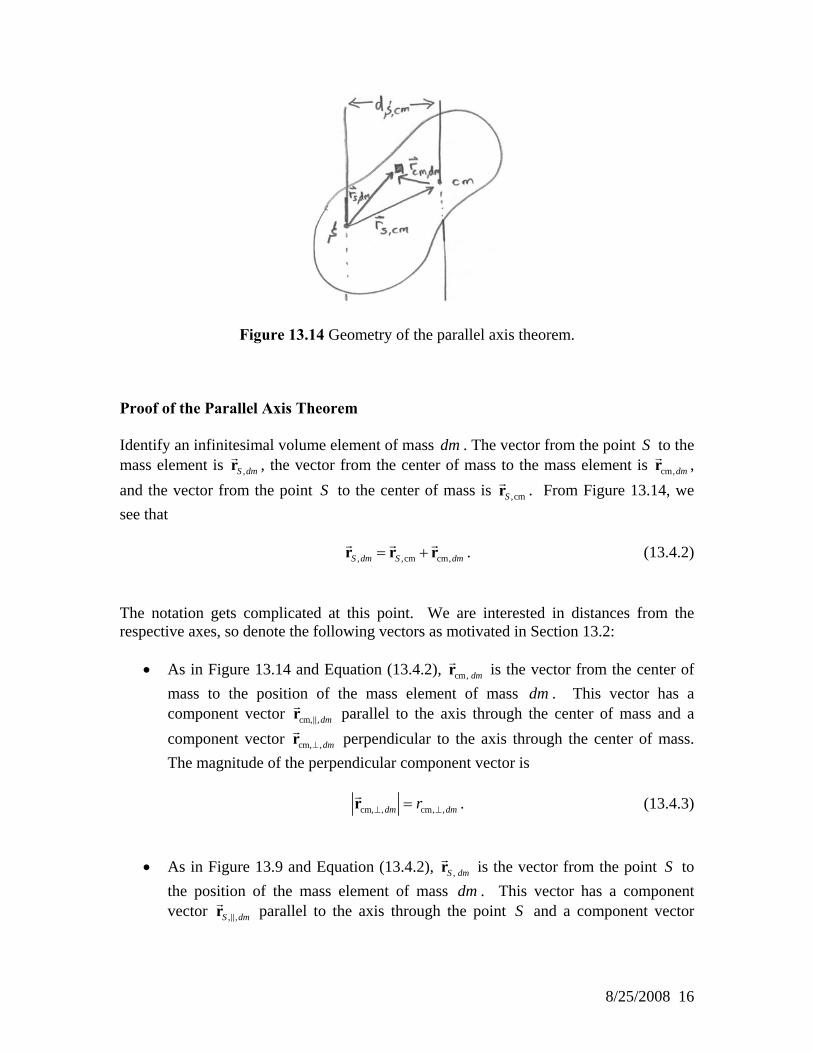
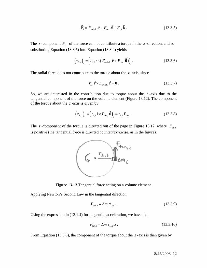
Figure 13.14 Geometry of the parallel axis theorem. Proof of the Parallel Axis Theorem Identify an infinitesimal volume element of mass . The vector from the point to the mass element is , the vector from the center of mass to the mass element is

dm S ,S dmr cm,dmr ,

and the vector from the point to the center of mass is S ,cmSr . From Figure 13.14, we see that , ,cm cm,S dm S dm= +r r r . (13.4.2) The notation gets complicated at this point. We are interested in distances from the respective axes, so denote the following vectors as motivated in Section 13.2:

• As in Figure 13.14 and Equation (13.4.2), cm, dmr is the vector from the center of mass to the position of the mass element of mass dm . This vector has a component vector parallel to the axis through the center of mass and a component vector perpendicular to the axis through the center of mass. The magnitude of the perpendicular component vector is

cm, ,dmr

cm, ,dm⊥r

cm, , cm, ,dm dmr⊥ =r ⊥ . (13.4.3)

• As in Figure 13.9 and Equation (13.4.2), ,S dmr is the vector from the point to the position of the mass element of mass . This vector has a component vector parallel to the axis through the point and a component vector

Sdm

, ,S dmr S

8/25/2008 16

, ,S dm⊥r perpendicular to the axis through the point . The magnitude of the perpendicular component vector is

S

, , , ,S dm S dmr⊥ ⊥=r . (13.4.4) • As in Figure 13.14 and Equation (13.4.2), ,cmSr is the vector from the point to

the center of mass. This vector has a component vector S

, ,cmSr parallel to both axes and a perpendicular component vector , ,cmS ⊥r of ,cmSr perpendicular to both axes (the axes are parallel, of course). The magnitude of the perpendicular component vector is

, ,cm ,cmS d⊥ =r S . (13.4.5) Equation (13.4.2) is now expressed as two equations,

, , , ,cm cm, ,

, , , ,cm cm, , .S dm S dm

S dm S dm

⊥ ⊥ ⊥= +

= +

r r r

r r r (13.4.6)

At this point, note that if we had simply decided that the two parallel axes are parallel to the -direction, we could have saved some steps and perhaps spared some of the notation with the triple subscripts. However, we want a more general result, one valid for cases where the axes are not fixed, or when different objects in the same problem have different axes. For example, consider the turning bicycle, for which the two wheel axes will not be parallel, or a spinning top that precesses (wobbles). Such cases will be considered in Chapter 16, and we will show the general case of the parallel axis theorem in anticipation of use for more general situations.

z

The moment of inertia about the point is S

( )2

, ,body

S SI dm r ⊥= ∫ dm

)dm

dm⊥

. (13.4.7)

From (13.4.6) we have

( )( ) (

( )

2

, , , , , ,

, ,cm cm, , , ,cm cm, ,

22,cm cm, , , ,cm cm, ,2 .

S dm S dm S dm

S dm S

S dm S

r

d r

⊥ ⊥ ⊥

⊥ ⊥ ⊥ ⊥

⊥ ⊥

= ⋅

= + ⋅ +

= + + ⋅

r r

r r r r

r r

(13.4.8)

Thus we have for the moment of inertia about S ,

8/25/2008 17

( ) ( ) ( )22,cm cm, , , ,cm cm, ,

body body body

2S S dm SI dm d dm r dm⊥ ⊥= + + ⋅∫ ∫ ∫ r r dm⊥ . (13.4.9)

In the first integral in Equation (13.4.9), , ,cm ,cmSr d⊥ S= is the distance between the parallel axes and is a constant and may be taken out of the integral, and ( )2

,cm ,cmbody

Sdm d m d=∫ 2S . (13.4.10)

The second term in Equation (13.4.9) is the moment of inertia about the axis through the center of mass,

( )2

cm cm, ,body

dmI dm r ⊥= ∫ . (13.4.11)

The third integral in Equation (13.4.9) is zero. To see this, note that the term is a constant and may be taken out of the integral,

, ,cmS ⊥r

( ) ( ), ,cm cm, , , ,cm cm, ,

body body

2 2S dm Sdm dm⊥ ⊥ ⊥ ⊥⋅ = ⋅∫ r r r r dm∫

)

(13.4.12)

The integral is the perpendicular component of the position of the center

of mass with respect to the center of mass, and hence

( cm, ,body

dmdm ⊥∫ r

0 , with the result that ( ), cm cm, ,

body

2 S dmdm ⊥ ⊥ 0⋅ =∫ r r . (13.4.13)

Thus, the moment of inertia about is just the sum of the first two integrals in Equation

S(13.4.9),

. (13.4.14) 2

cm ,cmSI I md= + S

13.3.1 Example: Uniform Rod, Part II Let point be the left end of the rod of Example 13.2.1 and Figure 13.13. Then the distance from the center of mass to the end of the rod is

S,cm / 2Sd L= . The moment of

inertia endSI I= about an axis passing through the endpoint is related to the moment of

8/25/2008 18

inertia about an axis passing through the center of mass, 2cm (1/12)I m L= , according to

Equation (13.4.14),

2 21 1 112 4 3S

2I m L m L m L= + = . (13.4.15)

In this case it’s easy and useful to check by direct calculation. Use Equation (13.3.20) but with the limits changed to 0x′ = and x L′ = , where / 2x x L′ = + ;

2 2end 0

body

3 3 32

0

( ) (0) 1 .3 3 3 3

L

L

I r dm x dx

x m L m m LL L

λ

λ

⊥ ′ ′= =

′= = − =

∫ ∫ (13.4.16)

13.5 Simple Pendulum and Physical Pendulum Simple Pendulum A pendulum consists of an object hanging from the end of a string or rigid rod pivoted about the point . The object is pulled to one side and allowed to oscillate. If the object has negligible size and the string or rod is massless, then the pendulum is called a simple pendulum. The force diagram for the simple pendulum is shown in Figure 13.15.

S

Figure 13.15 A simple pendulum.

8/25/2008 19

The string or rod exerts no torque about the pivot point S . The weight of the object has radial - and - components given by r̂ θ̂ ( )ˆˆcos sinm mg θ θ= −g r θ (13.5.1)

and the torque about the pivot point is given by S ( ),

ˆ ˆˆ ˆcos sin sinS S m m l m g l m gθ θ= × = × − = −r θg r rτ kθ (13.5.2)

and so the component of the torque in the z -direction (into the page in Figure 13.15 for θ positive, out of the page for θ negative) is ( ) sinS z

mglτ θ= − . (13.5.3) The moment of inertia of a point mass about the pivot point is S 2

SI ml= . (13.5.4) From Equation (13.3.15) the rotational dynamical equation is

( )

2

2

22

2sin .

S S Sz

dI Idt

dmgl mldt

θτ α

θθ

= =

− = (13.5.5)

Thus we have the equation of motion for the simple pendulum,

2

2 sind gdt lθ θ= − . (13.5.6)

When the angle of oscillation is small, then we can use the small angle approximation sinθ θ≅ ; (13.5.7) the rotational dynamical equation for the pendulum becomes

2

2

d gdt lθ θ≅ − . (13.5.8)

8/25/2008 20

This equation is similar to the object-spring simple harmonic oscillator differential equation from Chapter 10.2, Equation 10.2.3,

2

2

d x k xdt m

= − , (13.5.9)

which describes the oscillation of a mass about the equilibrium point of a spring. Recall that in Chapter 10.2, Equation 10.2.7, the angular frequency of oscillation was given by

springkm

ω = . (13.5.10)

By comparison, the frequency of oscillation for the pendulum is approximately

pendulumgl

ω ≅ , (13.5.11)

with period

pendulum

2 2 lTg

π πω

= ≅ . (13.5.12)

A procedure for determining the period for larger angles is given in Appendix 13.B. Physical Pendulum A physical pendulum consists of a rigid body that undergoes fixed axis rotation about a fixed point (Figure 13.16). The gravitational force acts at the center of mass of the physical pendulum (

SAppendix 13.A). Suppose the center of mass is a distance from

the pivot point . cml

S

8/25/2008 21

Figure 13.16 Physical pendulum.

The analysis is nearly identical to the simple pendulum. The torque about the pivot point is given by ( ),cm cm cm

ˆ ˆˆ ˆcos sin sinS S m l m g l m gθ θ= × = × − = −r θg r rτ θ k . (13.5.13)

Following the same steps that led from Equation (13.5.2) to Equation (13.5.6), the rotational dynamical equation for the physical pendulum is

( )

2

2

2

cm 2sin .

S S Sz

S

dI Idt

dmgl Idt

θτ α

θθ

= =

− = (13.5.14)

Thus we have the equation of motion for the physical pendulum,

2

cm2 sin

S

d mgldt Iθ θ= − . (13.5.15)

As with the simple pendulum, for small angles sinθ θ≈ and Equation (13.5.15) reduces to the simple harmonic oscillator equation with angular frequency

cmpendulum

S

mg lI

ω ≈ (13.5.16)

and period

physicalpendulum cm

2 2 SITm g l

π πω

= ≅ . (13.5.17)

It is sometimes convenient to express the moment of inertia about the pivot point in terms of and cml cmI using the parallel axis theorem in Equation (13.4.14), with ,cm cmSd l≡ ,

2cm cmSI I ml= + , with the result

cm cmphysical

cm

2 l ITg m g l

π≅ + . (13.5.18)

8/25/2008 22

Thus, if the object is “small” in the sense that 2cm cmI ml , the expressions for the

physical pendulum reduce to those for the simple pendulum. Note that this is not the case shown in Figure 13.16. 13.6 Torque and Rotational Work Introduction When a constant torque Sτ is applied to an object, and the object rotates through an angle θΔ about an axis through the center of mass, then the torque does an amount of work

SW τ θΔ = Δ on the object. By extension of the linear work-energy theorem, the amount of work done is equal to the change in the rotational kinetic energy of the object,

2 2rot cm cm 0 rot, rot,0

1 12 2f fW I I K Kω ω= − = − . (13.6.1)

The rate of doing this work is the rotational power exerted by the torque,

rot rotrot 0

lim S St

dW W dPdt t dt

θτ τ ωΔ →

Δ≡ = = =

Δ. (13.6.2)

Rotational work Consider a rigid body rotating about an axis. Each small element of mass in the rigid

body is moving in a circle of radius imΔ

( ),S ir ⊥ about the axis of rotation passing through the

point . Each mass element undergoes a small angular displacement S θΔ under the action of a tangential force, tan, tan,

ˆi F=F i θ , where θ̂ is the unit vector pointing in the

tangential direction (Figure 13.7). The element will then have an associated displacement vector for this motion, ( ), ,

ˆS i S ir θ

⊥Δ = Δr θ and the work done by the tangential force is

( ) ( )( ) ( )tan , , tan, , tan, ,

ˆ ˆi i S i i S i i S iW F r F rθ θ

⊥Δ = ⋅Δ = ⋅ Δ = ΔF r θ θ

⊥. (13.6.3)

Applying Newton’s Second Law to the element imΔ in the tangential direction, tan, tan,i iF m a i= Δ . (13.6.4) Using the expression in Equation (13.1.4) for tangential acceleration we have that

8/25/2008 23

( )tan, ,i i S iF m r α⊥

= Δ . (13.6.5)

Thus the rotational work done on the mass element is

( )2

,i i S iW m r α θ⊥

Δ = Δ Δ . (13.6.6)

Summing the rotational work done on all of the mass elements, we obtain

( )2

,i i S ii i

W W m r α θ⊥

⎛ ⎞Δ = Δ = Δ Δ⎜ ⎟

⎝ ⎠∑ ∑ . (13.6.7)

In the limit that the discrete mass elements become infinitesimal continuous mass elements, , the summation becomes an integral over the body: im dΔ → m

( ) ( )2 2

,body

i S i Si

W m r dm rα θ⊥⊥

⎛ ⎞⎛ ⎞Δ = Δ Δ → Δ⎜ ⎟⎜ ⎟ ⎜ ⎟⎝ ⎠ ⎝ ⎠

∑ ∫ α θ . (13.6.8)

Since the integral in this expression is just the moment of inertia about a fixed axis passing through the point , we have for the rotational work S SW I α θΔ = Δ . (13.6.9) Since the -component of the torque (in the direction along the axis of rotation) about S is given by

z

( )S Sz

Iτ α= , (13.6.10) the rotational work is the product of the torque and the angular displacement, ( )S z

W τ θΔ = Δ . (13.6.11) Recall the result of Equation (13.3.8) that the component of the torque (in the direction along the axis of rotation) about due to the tangential force, S tan,iF , acting on the mass element is imΔ ( ) ( ), tan, ,S i i S iz

F rτ⊥

= , (13.6.12)

and the total torque is the sum

8/25/2008 24

( ) ( ) ( ), tan,S S i iz zi i

F rτ τ ,S i ⊥= =∑ ∑ (13.6.13)

and so the work done is ( ) ( )tan, ,i i S i S z

i iW W F r θ τ⊥Δ = Δ = Δ = Δ∑ ∑ θ . (13.6.14)

In the limit of small angles, dθ θΔ → , W dWΔ → and the differential rotational work is ( )S z

dW dτ θ= . (13.6.15) We can integrate this amount of rotational work as the angle coordinate of the rigid body changes from some initial value 0θ θ= to some final value fθ θ= ,

( )0

f

S zW dW d

θ

θτ θ= =∫ ∫ . (13.6.16)

Rotational Kinetic Energy The general motion of a rigid body consists of a translation of the center of mass with velocity and a rotation about the center of mass with angular velocity cmv cmω . Having defined translational kinetic energy in Chapter 7.2, Equation 7.2.1, we now define the rotational kinetic energy for a rigid body about its center of mass. Each individual mass element undergoes circular motion about the center of mass with

angular frequency imΔ

cmω in a circle of radius ( )cm, ir⊥

. Therefore the velocity of each

element is given by ( )cm, cm, cmˆ

i ir ω⊥

=v θ . The rotational kinetic energy is then

( )22cm, cm, cm, cm

1 12 2i i i i iK m v m r 2ω

⊥= Δ = Δ . (13.6.17)

We now add up the kinetic energy for all the mass elements,

( ) ( )2 22 2

cm cm, cm, cm cm cmbody

2cm cm

1 12 2

1 .2

i i ii i

K K m r dm r

I

ω ω

ω

⊥⊥

⎛ ⎞⎛ ⎞= = Δ = ⎜ ⎟⎜ ⎟ ⎜ ⎟⎝ ⎠ ⎝

=

∑ ∑ ∫⎠ (13.6.18)

The total kinetic energy is the sum of the translational kinetic energy and the rotational kinetic energy,

8/25/2008 25

2total trans rot cm cm cm

1 12 2

K K K mv I 2ω= + = + . (13.6.19)

The above assertion that the total kinetic energy consists of two parts, which is certainly plausible, is derived in Appendix 13.C. Rotational Work-Kinetic Energy Theorem We will now show that the rotational work is equal to the change in rotational kinetic energy. We begin by substituting our result from Equation (13.6.10) into Equation (13.6.15) for the infinitesimal rotational work, rot SdW I dα θ= . (13.6.20) Recall that the rate of change of angular velocity is equal to the angular acceleration,

d dtα ω≡ and that the angular velocity is d dtω θ≡ . Note that in the limit of small displacements,

d dd d ddt dtω θθ ω= = ωω . (13.6.21)

Therefore the infinitesimal rotational work is

rot S S S Sd ddW I d I d I d I ddt dtω θα θ θ ω= = = = ωω . (13.6.22)

We can integrate this amount of rotational work as the angular velocity of the rigid body changes from some initial value 0ω ω= to some final value fω ω= ,

0

2rot rot 0

1 12 2

f

S S fW dW I d I Iω

ω2

Sω ω ω= = = −∫ ∫ ω . (13.6.23)

When a rigid body is rotating about a fixed axis passing through a point in the body, there is both rotation and translation about the center of mass unless is the center of mass. If we choose the point in the above equation for the rotational work to be the center of mass, then

SS

S

2 2rot cm cm, cm cm,0 rot, rot ,0 rot

1 12 2f fW I I K K Kω ω= − = − ≡ Δ . (13.6.24)

Recall the work-kinetic energy theorem stated that the total translational work done by all the forces is equal to the change in the translational kinetic energy of the center of mass,

8/25/2008 26

2 2trans cm, cm,0 trans

1 12 2fW mv mv K= − ≡ Δ . (13.6.25)

Since we did not include the effect of rotational work in Equation (13.6.25), we now add the two contributions to the total work and find that the total work done on a rigid body is equal to the total change of the kinetic energy

total trans rot

2 2 2cm, cm,0 cm cm 0

trans rot

1 1 1 12 2 2 2

.

f f

W W W

mv mv I I

K K

2ω ω

= +

⎛ ⎞ ⎛= − + −⎜ ⎟ ⎜⎝ ⎠ ⎝

= Δ + Δ

⎞⎟⎠

(13.6.26)

Rotational Power The rotational power is defined as the rate of doing rotational work,

rotrot

dWPdt

≡ . (13.6.27)

We can use our result for the infinitesimal work to find that the rotational power is the product of the applied torque with the angular velocity of the rigid body,

( ) ( )rotrot S Sz

dW dPdt dt z

θτ τ≡ = = ω . (13.6.28)

8/25/2008 27