Chapter 10 Pulse Characterization

Chapter 10

Pulse Characterization

Characterization of ultrashort laser pulses with pulse widths greater than20ps can be directly performed electronically using high speed photo detec-tors and sampling scopes. Photo detectors with bandwidth of 100 GHz areavailable. For shorter pulses usually some type of autocorrelation or cross-correlation in the optical domain using nonlinear optical effects has to beperformed, i.e. the pulse itself has to be used to measure its width, becausethere are no other controllable events available on such short time scales.

10.1 Intensity Autocorrelation

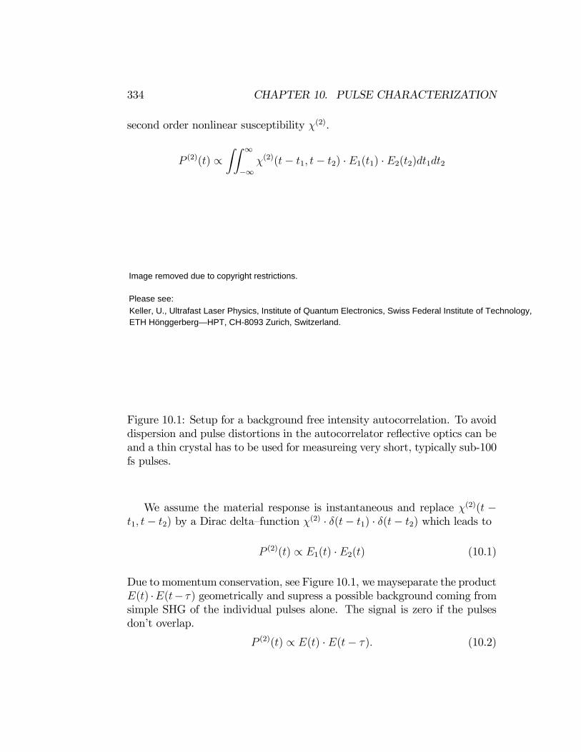
Pulse duration measurements using second-harmonic intensity autocorrela-tion is a standard method for pulse characterisation. Figure 10.1 shows thesetup for a background free intensity autocorrelation. The input pulse is splitin two, and one of the pulses is delayed by τ . The two pulses are focussedinto a nonliner optical crystal in a non-colinear fashion. The nonlinear opti-cal crystal is designed for efficient second harmonic generation over the fullbandwidth of the pulse, i.e. it has a large second order nonlinear opticalsuszeptibility and is phase matched for the specific wavelength range. Wedo not consider the z—dependence of the electric field and phase—matchingeffects. To simplify notation, we omit normalization factors. The inducednonlinear polarization is expressed as a convolution of two interfering electric—fields E1(t), E2(t) with the nonlinear response function of the medium, the

333

334 CHAPTER 10. PULSE CHARACTERIZATION

second order nonlinear susceptibility χ(2).

P (2)(t) ∝ZZ ∞

−∞χ(2)(t− t1, t− t2) ·E1(t1) · E2(t2)dt1dt2

Figure 10.1: Setup for a background free intensity autocorrelation. To avoiddispersion and pulse distortions in the autocorrelator reflective optics can beand a thin crystal has to be used for measureing very short, typically sub-100fs pulses.

We assume the material response is instantaneous and replace χ(2)(t −t1, t− t2) by a Dirac delta—function χ(2) · δ(t− t1) · δ(t− t2) which leads to

P (2)(t) ∝ E1(t) · E2(t) (10.1)

Due to momentum conservation, see Figure 10.1, we mayseparate the productE(t) ·E(t− τ) geometrically and supress a possible background coming fromsimple SHG of the individual pulses alone. The signal is zero if the pulsesdon’t overlap.

P (2)(t) ∝ E(t) · E(t− τ). (10.2)

Keller, U., Ultrafast Laser Physics, Institute of Quantum Electronics, Swiss Federal Institute of Technology, ETH Hönggerberg—HPT, CH-8093 Zurich, Switzerland.

Image removed due to copyright restrictions. Please see:

10.1. INTENSITY AUTOCORRELATION 335

Table 10.1: Pulse shapes and its deconvolution factors

relating FWHM, τ p, of the pulse to FWHM, τA, of the

intensity autocorrelationfunction.

The electric field of the second harmonic radiation is directly proportional tothe polarization, assuming a nondepleted fundamental radiation and the useof thin crystals. Due to momentum conservation, see Figure 10.1, we find

IAC(τ) ∝Z ∞

−∞

¯A(t)A(t− τ)

¯2dt . (10.3)

∝Z ∞

−∞I(t)I(t− τ) dt, (10.4)




with the complex envelopeA(t) and intensity I(t) = |A(t)|2 of the input pulse.The photo detector integrates because its response is usually much slowerthan the pulsewidth. Note, that the intenisty autocorrelation is symmetricby construction

IAC(τ) = IAC(−τ). (10.5)

It is obvious from Eq.(10.3) that the intensity autocorrelation does not con-tain full information about the electric field of the pulse, since the phase ofthe pulse in the time domain is completely lost. However, if the pulse shapeis known the pulse width can be extracted by deconvolution of the correla-tion function. Table 10.1 gives the deconvolution factors for some often usedpulse shapes.

10.2 Interferometric Autocorrelation (IAC)

A pulse characterization method, that also reveals the phase of the pulseis the interferometric autocorrelation introduced by J. C. Diels [2], (Figure10.2 a). The input beam is again split into two and one of them is delayed.However, now the two pulses are sent colinearly into the nonlinear crystal.Only the SHG component is detected after the filter.

Figure 10.2: (a) Setup for an interferometric autocorrelation. (b) Delaystage, so that both beams are reflected from the same air/medium interfaceimposing the same phase shifts on both pulses.



10.2. INTERFEROMETRIC AUTOCORRELATION (IAC) 337

The total field E(t, τ) after the Michelson-Interferometer is given by thetwo identical pulses delayed by τ with respect to each other

E(t, τ) = E(t+ τ) +E(t) (10.6)

= A(t+ τ)ejω⊂(t+τ)ejφCE +A(t)ejωctejφCE . (10.7)

A(t) is the complex amplitude, the term eiω0t describes the oscillation withthe carrier frequency ω0 and φCE is the carrier-envelope phase. Eq. (10.1)writes

P (2)(t, τ) ∝ ¡A(t+ τ)ejωc(t+τ)ejφCE +A(t)ejωctejφCE¢2

(10.8)

This is only idealy the case if the paths for both beams are identical. Iffor example dielectric or metal beamsplitters are used, there are differentreflections involved in the Michelson-Interferometer shown in Fig. 10.2 (a)leading to a differential phase shift between the two pulses. This can beavoided by an exactly symmetric delay stage as shown in Fig. 10.1 (b).Again, the radiated second harmonic electric field is proportional to the

polarization

E(t, τ) ∝ ¡A(t+ τ)ejωc(t+τ)ejφCE +A(t)ejωc(t)ejφCE¢2. (10.9)

The photo—detector (or photomultiplier) integrates over the envelope of eachindividual pulse

I(τ) ∝Z ∞

−∞

¯ ¡A(t+ τ)ejωc(t+τ) +A(t)ejωct

¢2 ¯2dt .

∝Z ∞

−∞

¯A2(t+ τ)ej2ωc(t+τ)

+2A(t+ τ)A(t)ejωc(t+τ)ejωct

+A2(t)ej2ωct¯2. (10.10)

Evaluation of the absolute square leads to the following expression

I(τ) ∝Z ∞

−∞

h|A(t+ τ)|4 + 4|A(t+ τ)|2|A(t)|2 + |A(t)|4

+2A(t+ τ)|A(t)|2A∗(t)ejωcτ + c.c.+2A(t)|A(t+ τ)|2A∗(t+ τ)e−jωcτ + c.c.

+A2(t+ τ)(A∗(t))2ej2ωcτ + c.c.idt . (10.11)


The carrier—envelope phase φCE drops out since it is identical to both pulses.The interferometric autocorrelation function is composed of the followingterms

I(τ) = Iback + Iint(τ) + Iω(τ) + I2ω(τ) . (10.12)

Background signal Iback:

Iback =

Z ∞

−∞

¡|A(t+ τ)|4 + |A(t)|4¢ dt = 2

Z ∞

−∞I2(t) dt (10.13)

Intensity autocorrelation Iint(τ):

Iint(τ) = 4

Z ∞

−∞|A(t+ τ)|2|A(t)|2 dt = 4

Z ∞

−∞I(t+ τ) · I(t) dt (10.14)

Coherence term oscillating with ωc: Iω(τ):

Iω(τ) = 4

Z ∞

−∞Rehµ

I(t) + I(t+ τ)

¶A∗(t)A(t+ τ)ejωτ

idt (10.15)

Coherence term oscillating with 2ωc: I2ω(τ):

Iω(τ) = 2

Z ∞

−∞RehA2(t)(A∗(t+ τ))2ej2ωτ

idt (10.16)

Eq. (10.12) is often normalized relative to the background intensity Ibackresulting in the interferometric autocorrelation trace

IIAC(τ) = 1 +Iint(τ)

Iback+

Iω(τ)

Iback+

I2ω(τ)

Iback. (10.17)

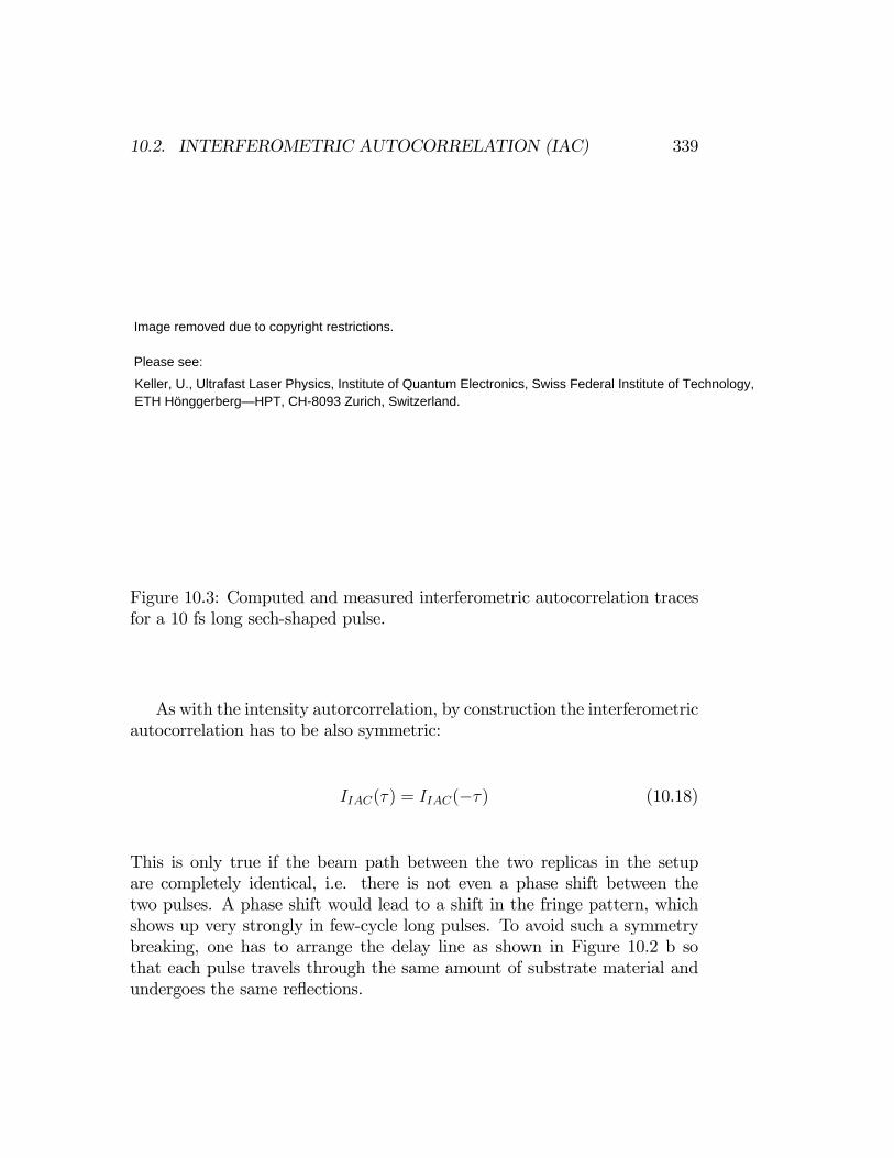
Eq. (10.17) is the final equation for the normalized interferometric auto-correlation. The term Iint(τ) is the intensity autocorrelation, measured bynon—colinear second harmonic generation as discussed before. Therefore, theaveraged interferometric autocorrelation results in the intensity autocorrela-tion sitting on a background of 1.Fig. 10.3 shows a calculated and measured IAC for a sech-shaped pulse.


Figure 10.3: Computed and measured interferometric autocorrelation tracesfor a 10 fs long sech-shaped pulse.

As with the intensity autorcorrelation, by construction the interferometricautocorrelation has to be also symmetric:

IIAC(τ) = IIAC(−τ) (10.18)

This is only true if the beam path between the two replicas in the setupare completely identical, i.e. there is not even a phase shift between thetwo pulses. A phase shift would lead to a shift in the fringe pattern, whichshows up very strongly in few-cycle long pulses. To avoid such a symmetrybreaking, one has to arrange the delay line as shown in Figure 10.2 b sothat each pulse travels through the same amount of substrate material andundergoes the same reflections.




At τ = 0, all integrals are identical

Iback ≡ 2Z|A(t)|4dt

Iint(τ = 0) ≡ 2Z|A2(t)|2dt = 2

Z|A(t)|4dt = Iback

Iω(τ = 0) ≡ 2Z|A(t)|2A(t)A∗(t)dt = 2

Z|A(t)|4dt = Iback

I2ω(τ = 0) ≡ 2Z

A2(t)(A2(t)∗dt = 2

Z|A(t)|4dt = Iback

(10.19)

Then, we obtain for the interferometric autocorrelation at zero time delay

IIAC(τ)|max = IIAC(0) = 8

IIAC(τ → ±∞) = 1

IIAC(τ)|min = 0

(10.20)

This is the important 1:8 ratio between the wings and the pick of the IAC,which is a good guide for proper alignment of an interferometric autocorre-lator. For a chirped pulse the envelope is not any longer real. A chirp in thepulse results in nodes in the IAC. Figure 10.4 shows the IAC of a chirpedsech-pulse

A(t) =

µsech

µt

τ p

¶¶(1+jβ)

for different chirps.


Figure 10.4: Influence of increasing chirp on the IAC.

10.2.1 Interferometric Autocorrelation of an UnchirpedSech-Pulse

Envelope of an unchirped sech-pulse

A(t) = sech(t/τ p) (10.21)

Interferometric autocorrelation of a sech-pulse

IIAC(τ) = 1 + 2 + cos (2ωcτ)3³³

ττp

´cosh

³ττp

´− sinh

³ττp

´´sinh3

³ττp

´ (10.22)

+3³sinh

³2ττp

´−³2ττp

´´sinh3

³ττp

´ cos(ωcτ)




10.2.2 Interferometric Autocorrelation of a ChirpedGaussian Pulse

Complex envelope of a Gaussian pulse

A(t) = exp

∙−12

µt

tp

¶(1 + jβ)

¸. (10.23)

Interferometric autocorrelation of a Gaussian pulse

IIAC(τ) = 1 +

½2 + e

−β2

2

³ττp

´2cos(2ωcτ)

¾e−12

³ττp

´2(10.24)

+4e− 3+β2

8

³ττp

´2cos

Ãβ

4

µτ

τ p

¶2!cos (ωcτ) .

10.2.3 Second Order Dispersion

It is fairly simple to compute in the Fourier domain what happens in thepresence of dispersion.

E(t) = A(t)ejωctF−→ E(ω) (10.25)

After propagation through a dispersive medium we obtain in the Fourierdomain.

E0(ω) = E(ω)e−iΦ(ω)

and

E0(t) = A0(t)ejωct

Figure 10.5 shows the pulse amplitude before and after propagation througha medium with second order dispersion. The pulse broadens due to the dis-persion. If the dispersion is further increased the broadening increases andthe interferometric autocorrelation traces shown in Figure 10.5 develope acharacteristic pedestal due to the term Iint. The width of the interferomet-rically sensitive part remains the same and is more related to the coherencetime in the pulse, that is proportional to the inverse spectral width and doesnot change.


Figure 10.5: Effect of various amounts of second order dispersion on a trans-form limited 10 fs Sech-pulse.

10.2.4 Third Order Dispersion

We expect, that third order dispersion affects the pulse significantly for

D3

τ 3> 1

which is for a 10fs sech-pulse D3 >¡10 fs1.76

¢3˜183 fs3. Figure 10.6 and 10.7

show the impact on pulse shape and interferometric autocorrelation. Theodd dispersion term generates asymmetry in the pulse. The interferometricautocorrelation developes characteristic nodes in the wings.




Figure 10.6: Impact of 200 fs3 third order dispersion on a 10 fs pulse at acenter wavelength of 800 nm.and its interferometric autocorrelation.

Figure 10.7: Changes due to increasing third order Dispersion from 100-1000fs3on a 10 fs pulse at a center wavelength of 800 nm.






10.2.5 Self-Phase Modulation

Self-phase modulation without compensation by proper negative dispersiongenerates a phase over the pulse in the time domain. This phase is invisiblein the intensity autocorrelation, however it shows up clearly in the IAC, seeFigure 10.8 for a Gaussian pulse with a peak nonlinear phase shift φ0 =δA20 = 2 and Figure 10.8 for a nonlinear phase shift φ0 = 3.

Figure 10.8: Change in pulse shape and interferometric autocorrelation ina 10 fs pulse at 800 nm subject to pure self-phase modulation leading to anonlinear phase shift of φ0 = 2.




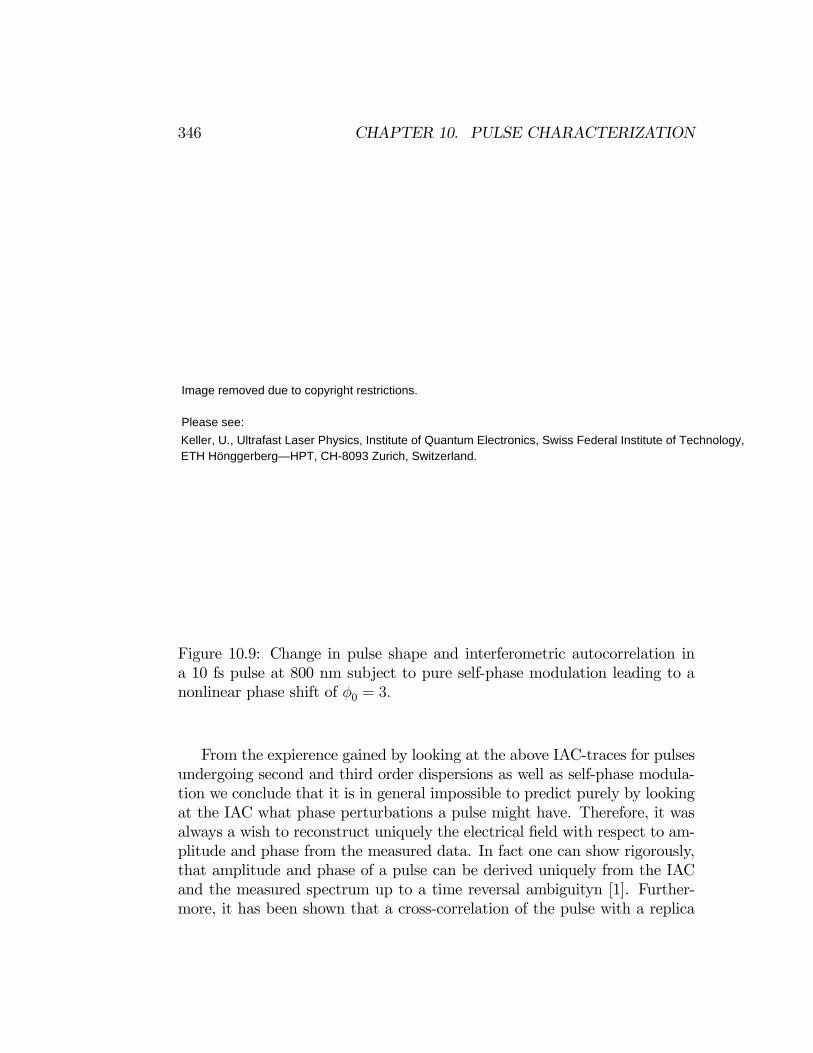
Figure 10.9: Change in pulse shape and interferometric autocorrelation ina 10 fs pulse at 800 nm subject to pure self-phase modulation leading to anonlinear phase shift of φ0 = 3.

From the expierence gained by looking at the above IAC-traces for pulsesundergoing second and third order dispersions as well as self-phase modula-tion we conclude that it is in general impossible to predict purely by lookingat the IAC what phase perturbations a pulse might have. Therefore, it wasalways a wish to reconstruct uniquely the electrical field with respect to am-plitude and phase from the measured data. In fact one can show rigorously,that amplitude and phase of a pulse can be derived uniquely from the IACand the measured spectrum up to a time reversal ambiguityn [1]. Further-more, it has been shown that a cross-correlation of the pulse with a replica



10.3. FREQUENCY RESOLVED OPTICAL GATING (FROG) 347

chirped in a known medium and the pulse spectrum is enough to reconstructthe pulse [3]. Since the spectrum of the pulse is already given only the phasehas to be determined. If a certain phase is assumed, the electric field andthe measured cross-correlation or IAC can be computed. Minimization ofthe error between the measured cross-correlation or IAC will give the de-sired spectral phase. This procedure has been dubbed PICASO (Phase andIntenisty from Cross Correlation and Spectrum Only).

Note, also instead of measuring the autocorrelation and interferometricautocorrelation with SHG one can also use two-photon absorption or higherorder absorption in a semiconductor material (Laser or LED) [4].

However today, the two widely used pulse chracterization techniques areFrequency Resolved Optical Gating (FROG) and Spectral Phase Interferom-etry for Direct Electric Field Reconstruction (SPIDER)

10.3 Frequency Resolved Optical Gating (FROG)

We follow closely the bock of the FROG inventor Rich Trebino. In frequencyresolved optical gating, the pulse to be characterized is gated by anotherultrashort pulse [5]. The gating is no simple linear sampling technique, butthe pulses are crossed in a medium with an instantaneous nonlinearity (χ(2)

or χ(3)) in the same way as in an autocorrelation measurement (Figures 10.1and 10.10). The FROG—signal is a convolution of the unknown electric—fieldE(t) with the gating—field g(t) (often a copy of the unknown pulse itself).However, after the interaction of the pulse to be measured and the gatepulse, the emitted nonlinear optical radiation is not put into a simple photodetector, but is instead spectrally resolved detected. The general form of thefrequency—resolved intensity, or Spectrogram SF (τ , ω) is given by

SF (τ , ω) ∝¯Z ∞

−∞E(t) · g(t− τ)e−jω tdt

¯2. (10.26)


Figure 10.10: The spectrogram of a waveform E(t) tells the intensity andfrequency in a given time interval [5].

Representations of signals, or waveforms in general, by time-frequencydistributions has a long history. Most notabley musical scores are a temporalsequence of tones giving its frequency and volume, see Fig. 10.11.

Figure 10.11: A musical score is a time-frequency representation of the signalto be played.

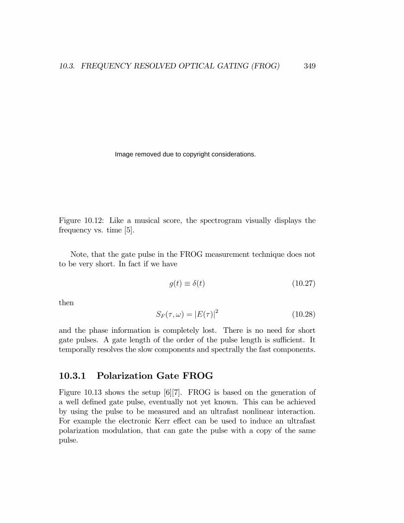
Time-frequency representations are well known in the radar community,signal processing and quantummechanics [9] (Spectrogram, Wigner-Distribution,Husimi-Distribution, ...), Figure 10.12 shows the spectrogram of differentlychirped pulses. Like a mucical score, the spectrogram visually displays thefrequency vs. time.

Image removed due to copyright considerations.


Figure 10.12: Like a musical score, the spectrogram visually displays thefrequency vs. time [5].

Note, that the gate pulse in the FROG measurement technique does notto be very short. In fact if we have

g(t) ≡ δ(t) (10.27)

then

SF (τ , ω) = |E(τ)|2 (10.28)

and the phase information is completely lost. There is no need for shortgate pulses. A gate length of the order of the pulse length is sufficient. Ittemporally resolves the slow components and spectrally the fast components.

10.3.1 Polarization Gate FROG

Figure 10.13 shows the setup [6][7]. FROG is based on the generation ofa well defined gate pulse, eventually not yet known. This can be achievedby using the pulse to be measured and an ultrafast nonlinear interaction.For example the electronic Kerr effect can be used to induce an ultrafastpolarization modulation, that can gate the pulse with a copy of the samepulse.



Figure 10.13: Polarization Gate FROG setup. The instantaneous Kerr-effectis used to rotate the polarization of the signal pulse E(t) during the presenceof the gate pulse E(t− τ) proportional to the intensity of the gate pulse [5].

The signal analyzed in the FROG trace is, see Figure 10.14,

Esig(t, τ) = E(t) |E(t− τ)|2 (10.29)

Figure 10.14: The signal pulse reflects the color of the gated pulse at thetime 2τ/3 [5]


Variable Delay

Pulse to be Measured

Beam Splitter

E(t-τ)

E(t)

Spectro-meter

CameraWave Plate (45o rotation of polarization)

Instantaneous NonlinearOptical Medium

Esig(t,τ) ∝ E(t) |E(t-τ)|2

IFROG(ω,τ) = |∫Esig(t,τ) e-iwtdt|2

"Polarization-Gate" Geometry

Figure by MIT OCW.


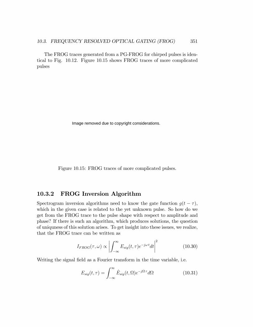
The FROG traces generated from a PG-FROG for chirped pulses is iden-tical to Fig. 10.12. Figure 10.15 shows FROG traces of more complicatedpulses

Figure 10.15: FROG traces of more complicated pulses.

10.3.2 FROG Inversion Algorithm

Spectrogram inversion algorithms need to know the gate function g(t − τ),which in the given case is related to the yet unknown pulse. So how do weget from the FROG trace to the pulse shape with respect to amplitude andphase? If there is such an algorithm, which produces solutions, the questionof uniquness of this solution arises. To get insight into these issues, we realize,that the FROG trace can be written as

IFROG(τ , ω) ∝¯Z ∞

−∞Esig(t, τ)e

−jω tdt

¯2(10.30)

Writing the signal field as a Fourier transform in the time variable, i.e.

Esig(t, τ) =

Z ∞

−∞Esig(t,Ω)e

−jΩ τdΩ (10.31)



yields

IFROG(τ , ω) ∝¯Z ∞

−∞

Z ∞

−∞Esig(t,Ω)e

−jω t−jΩ τdtdΩ

¯2. (10.32)

This equation shows that the FROG-trace is the magnitude square of a two-dimensional Fourier transform related to the signal field Esig(t, τ). The in-version of Eq.(10.32) is known as the 2D-phase retrival problem. Fortunatelyalgorithms for this inversion exist [8] and it is known that the magnitude (ormagnitude square) of a 2D-Fourier transform (FT) essentially uniquely de-termines also its phase, if additional conditions, such as finite support or therelationship (10.29) is given. Essentially unique means, that there are ambi-guities but they are not dense in the function space of possible 2D-transforms,i.e. they have probability zero to occur.Furthermore, the unknown pulse E(t) can be easily obtained from the

modified signal field Esig(t,Ω) because

Esig(t,Ω) =

Z ∞

−∞Esig(t, τ)e

jΩ τdτ (10.33)

=

Z ∞

−∞E(t)g(t− τ)e−jΩ τdτ (10.34)

= E(t)G∗(Ω)e−jΩ t (10.35)

with

G(Ω) =

Z ∞

−∞g(τ)e−jΩ τdτ. (10.36)

Thus there is

E(t) ∝ Esig(t, 0). (10.37)

The only condition is that the gate function should be chosen such thatG(Ω) 6= 0. This is very powerful.

Fourier Transform Algorithm

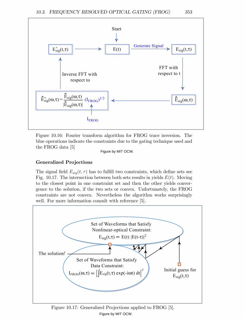
The Fourier transform algorithm also commonly used in other phase retrievalproblems is schematically shown in Fig. 10.16


Figure 10.16: Fourier transform algorithm for FROG trace inversion. Theblue operations indicate the constraints due to the gating technique used andthe FROG data [5]

Generalized Projections

The signal field Esig(t, τ) has to fulfill two constraints, which define sets seeFig. 10.17. The intersection between both sets results in yields E(t). Movingto the closest point in one constraint set and then the other yields conver-gence to the solution, if the two sets or convex. Unfortunately, the FROGconstraints are not convex. Nevertheless the algorithm works surprisinglywell. For more information consult with reference [5].

Figure 10.17: Generalized Projections applied to FROG [5].

E(t) Esig(t,τ)Esig(t,τ)

Start

Inverse FFT with respect to

Generate Signal

FFT with respect to t

Esig(ω,τ) (IFROG)1/2

IFROG

= Esig(ω,τ)

|Esig(ω,τ)|Esig(ω,τ)

Set of Waveforms that Satisfy Nonlinear-optical Constraint:

Set of Waveforms that Satisfy Data Constraint:

The solution!

Initial guess for Esig(t,τ)

Esig(t,τ) ∝ E(t) |E(t-τ)|2

IFROG(ω,τ) ∝ |∫Esig(t,τ) exp(-iωt) dt|2

Figure by MIT OCW.

Figure by MIT OCW.


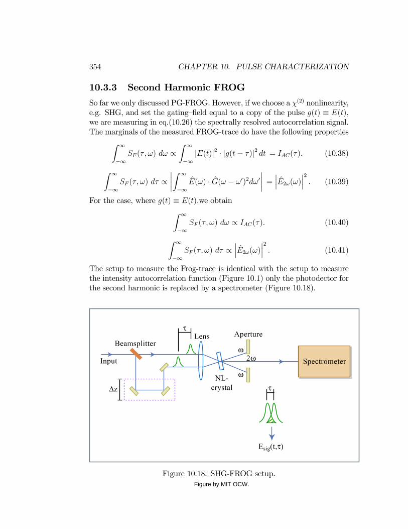
10.3.3 Second Harmonic FROG

So far we only discussed PG-FROG. However, if we choose a χ(2) nonlinearity,e.g. SHG, and set the gating—field equal to a copy of the pulse g(t) ≡ E(t),we are measuring in eq.(10.26) the spectrally resolved autocorrelation signal.The marginals of the measured FROG-trace do have the following propertiesZ ∞

−∞SF (τ , ω) dω ∝

Z ∞

−∞|E(t)|2 · |g(t− τ)|2 dt = IAC(τ). (10.38)

Z ∞

−∞SF (τ , ω) dτ ∝

¯Z ∞

−∞E(ω) · G(ω − ω0)2dω0

¯=¯E2ω(ω)

¯2. (10.39)

For the case, where g(t) ≡ E(t),we obtainZ ∞

−∞SF (τ , ω) dω ∝ IAC(τ). (10.40)

Z ∞

−∞SF (τ , ω) dτ ∝

¯E2ω(ω)

¯2. (10.41)

The setup to measure the Frog-trace is identical with the setup to measurethe intensity autocorrelation function (Figure 10.1) only the photodector forthe second harmonic is replaced by a spectrometer (Figure 10.18).

Figure 10.18: SHG-FROG setup.

∆z

τ

τ

ω

ω2ωInput

BeamsplitterLens

NL-crystal

Aperture

Esig(t,τ)

Spectrometer

Figure by MIT OCW.


Since the intensity autocorrelation function and the integrated spectrumcan be measured simultaneously, this gives redundancy to check the correct-ness of all measurements via the marginals (10.38, 10.39). Figure 10.19 showsthe SHG-FROG trace of the shortest pulses measured sofar with FROG.

Figure 10.19: FROG measurement of a 4.5 fs laser pulse.

Baltuska, Pshenichnikov, and Wiersma. Journal of Quantum Electronics 35 (1999): 459.



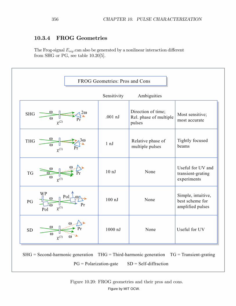
Figure 10.20: FROG geometries and their pros and cons.

SHG

Sensitivity Ambiguities

SHG = Second-harmonic generation

.001 nJDirection of time;Rel. phase of multiplepulses

Most sensitive;most accurate

Tightly focused beams

Useful for UV and transient-gratingexperiments

Simple, intuitive, best scheme for amplified pulses

Useful for UV

Relative phase of multiple pulses

None

None

None

1 nJ

10 nJ

100 nJ

1000 nJ

THG = Third-harmonic generation TG = Transient-grating

PG = Polarization-gate SD = Self-diffraction

χ(2)

χ(3)

χ(3)

χ(3)

χ(3)

Pr

ω 2ω

3ω

ω

THG

TG

PG

SD

Pol

WP

Pr

Pr

Pr

Pr

Pol

ω

ω

ω

ω

ωω

ω

ω

ω

ω

ω

ω

ω

FROG Geometries: Pros and Cons

10.3.4 FROG Geometries

The Frog-signal Esig.can also be generated by a nonlinear interaction differentfrom SHG or PG, see table 10.20[5].

Figure by MIT OCW.

10.4. SPECTRAL INTERFEROMETRY AND SPIDER 357

10.4 Spectral Interferometry and SPIDER

Spectral Phase Interferometry for Direct Electric—Field Reconstruction (SPI-DER) avoids iterative reconstruction of the phase profile. Iterative Fouriertransform algorithms do have the disadvantage of sometimes being rathertime consuming, preventing real—time pulse characterization. In addition,for “pathological" pulse forms, reconstruction is difficult or even impossible.It is mathematically not proven that the retrieval algorithms are unambigu-ous especially in the presence of noise.Spectral shearing interferometry provides an elegant method to overcome

these disadvantages. This technique has been first introduced by C. Iaconisand I.A. Walmsley in 1999 [11] and called spectral phase interferometry fordirect electric—field reconstruction — SPIDER. Before we discuss SPIDER letslook at spectral interferometry in general

10.4.1 Spectral Interferometry

The spectrum of a pulse can easily be measured with a spectrometer. Thepulse would be completely know, if we could determine the phase acrossthe spectrum. To determine this unknown phase spectral interferometry forpulse measurement has been proposed early on by Froehly and others [12].If we would have a well referenced pulse with field ER(t), superimpose theunknown electric field ES(t) delayed with the reference pulse and interferethem in a spectrometer, see Figure 10.21, we obtain for the spectrometeroutput

EI(t) = ER(t) +ES(t− τ) (10.42)

S(ω) =

¯Z +∞

−∞EI(t)e

−jωtdt

¯2=¯ER(ω) + ES(ω)

−jωτ¯2

(10.43)

= SDC(ω) + S(−)(ω)ejωτ + S(+)(ω)e−jωτ (10.44)

with

S(+)(ω) = E∗R(ω)ES(ω) (10.45)

S(−)(ω) = S(+)∗(ω) (10.46)

Where (+) and (-) indicate as before, well separted positive and negative"frequency" signals, where "frequency" is now related to τ rather than ω.


Figure 10.21: Spectral Interferometery of a signal pulse with a referencepulse.

If τ is chosen large enough, the inverse Fourier transformed spectrumS(t) = F−1S(ω) results in well separated signals, see Figure 10.22.

S(t) = SDC(t) + S(−)(t+ τ) + S(+)(t− τ) (10.47)

Figure 10.22: Decomposition of SPIDER signal.

We can isolate either the positive or negative frequency term with a filterin the time domain. Back transformation of the corresponding term to thefrequency domain and computation of the spectral phase of one of the termsresults in the spectral phase of the signal up to the known phase of thereference pulse and a linear phase contribution from the delay.

Φ(+)(ω) = argS(+)(ω)ejωτ = ϕS(ω)− ϕR(ω) + ωτ (10.48)

Spectrometer

Frequency

ER(t)

ES(t-τ)

1/τ

-τ τ0

S(-)(t) S(+)(t)

SDC(t)

S(t)

t

Figure by MIT OCW.

Figure by MIT OCW.


Figure 10.23: The principle of operation of SPIDER.

Adapted from F. X. Kaertner. Few-Cycle Laser Pulse Generation and its Applications. New York, NY: Springer-Verlag, 2004..

10.4.2 SPIDER

What can we do if we don’t have a well characterized reference pulse? C.Iaconis and I.A. Walmsley [?] came up with the idea of generating two up-converted spectra slightly shifted in frequency and to investigate the spectralinterference of these two copies, see Figure 10.23. We use

ER(t) = E(t)ejωSt (10.49)

ES(t) = E(t− τ)ej(ωS+Ω)t (10.50)

EI(t) = ER(t) +ES(t) (10.51)

where ωs and ωs + Ω are the two frequencies used for upconversion and Ωis called the spectral shear between the two pulses. E(t) is the unknownelectric field with spectrum

E(ω) =¯E(ω)

¯ejϕ(ω) (10.52)

Spectral interferometry using these specially constructed signal and referencepulses results in

S(ω) =

¯Z +∞

−∞EI(t)e

−jωtdt

¯2= SDC(ω)+S

(−)(ω)ejωτ+S(+)(ω)e−jωτ (10.53)


S(+)(ω) = E∗R(ω)ES(ω) = E∗(ω − ωs)E(ω − ωs − Ω) (10.54)

S(−)(ω) = S(+)∗(ω) (10.55)

The phase ψ(ω) = arg[S(+)(ω)e−jωτ ] derived from the isolated positive spec-tral component is

ψ(ω) = ϕ(ω − ωs − Ω)− ϕ(ω − ωs)− ωτ. (10.56)

The linear phase ωτ can be substracted off after independent determinationof the time delay τ . It is obvious that the spectral shear Ω has to be smallcompared to the spectral bandwdith ∆ω of the pulse, see Fig. 10.23. Thenthe phase difference in Eq.(10.56) is proportional to the group delay in thepulse, i.e.

−Ωdϕ

dω= ψ(ω), (10.57)

or

ϕ(ω) = − 1Ω

Z ω

0

ψ(ω0)dω0. (10.58)

Note, an error ∆τ in the calibration of the time delay τ results in an errorin the chirp of the pulse

∆ϕ(ω) = −ω2

2Ω∆τ . (10.59)

Thus it is important to chose a spectral shear Ω that is not too small. Howsmall does it need to be? We essentially sample the phase with a samplespacing Ω. The Nyquist theorem states that we can uniquely resolve a pulsein the time domain if it is only nonzero over a length [−T, T ], where T = π/Ω.On the other side the shear Ω has to be large enough so that the fringes inthe spectrum can be resolved with the available spectrometer.


Figure 10.24: SPIDER setup; SF10: 65mm glass block (GDD/z ≈160 fs2/mm), BS: metallic beam splitters (≈ 200µm, Cr—Ni coating 100nm),τ : adjustable delay between the unchirped replica, τSHG: delay betweenunchirped pulses and strongly chirp pulse, RO: reflective objective (Ealing—Coherent, x35, NA=0.5, f=5.4mm), TO: refractive objective , L: lens, spec-trometer: Lot-Oriel MS260i, grating: 400 l/mm, Blaze—angle 350nm, CCD:Andor DU420 CCI 010, 1024 x 255 pixels, 26µm/pixel [13].

Generation of two replica without additional chirp:

A Michelson—type interferometer generates two unchirped replicas. Thebeam—splitters BS have to be broadband, not to distort the pulses. Thedelay τ between the two replica has to be properly chosen, i.e. in the setupshown it was about 400-500 fs corresponding to 120-150 µm distance in space.

Courtesy of Richard Ell. Used with permission.

SPIDER Setup

We follow the work of Gallmann et al. [?] that can be used for characteri-zation of pulses only a few optical cycles in duration. The setup is shown inFigure 10.24.


Spectral shearing:

The spectrally sheared copies of the pulse are generated by sum-frequencygeneration (SFG) with quasi-monochromatic beams at frequencies ωs andωs + Ω. These quasi monochromatic signals are generated by strong chirp-ing of a third replica (cf. Fig. 10.24) of the signal pulse that propagatesthrough a strongly dispersive glass slab. For the current setup we estimatefor the broadening of a Gaussian pulse due to the glass dispersion from 5 fsto approximately 6ps. Such a stretching of more than a factor of thou-sand assures that SFG occurs within an optical bandwidth less than 1nm, aquasi—monochromatic signal. Adjustment of the temporal overlap τSHG withthe two unchirped replica is possible by a second delay line. The strechedpulse can be computed by propagation of the signal pulse E(t) through thestrongly dispersive medium with transfer characteristic

Hglass(ω) = e−jDglass(ω−ωc)2/2 (10.60)

neglecting linear group delay and higher order dispersion terms. We otain forthe analytic part of the electric field of the streched pulse leaving the glassblock by convolution with the transfer characteristic

Estretch(t) =

+∞Z−∞

E(ω)e−jDglass(ω−ωc)2/2ejωtdω = (10.61)

= ejt2/(2Dglass)ejωct

+∞Z−∞

E(ω)e−jDglass((ω−ωc)−t/Dglass2)/2dω(10.62)

If the spectrum of the pulse is smooth enough, the stationary phase methodcan be applied for evaluation of the integral and we obtain

Estretch(t) ∝ ejωc(t+t2/(2Dglass)E(ω = ωc + t/Dglass) (10.63)

Thus the field strength at the position where the instantaneous frequency is

ωinst =d

dtωc(t+ t2/(2Dglass) = ωc + t/Dglass (10.64)

is given by the spectral amplitude at that frequency, E(ω = ωc + t/Dglass).For large stretching, i.e.

|τ p/Dglass| ¿ |Ω| (10.65)

the up-conversion can be assumed to be quasi monochromatic.


SFG:

A BBO crystal (wedged 10—50µm) is used for type I phase—matched SFG.Type II phase—matching would allow for higher acceptance bandwidths. Thepulses are focused into the BBO—crystal by a reflective objective composed ofcurved mirrors. The signal is collimated by another objective. Due to SFGwith the chirped pulse the spectral shear is related to the delay between bothpulses, τ , determined by Eq.(10.64) to be

Ω = −τ/Dglass. (10.66)

Note, that conditions (10.65) and (10.66) are consistent with the fact thatthe delay between the two pulses should be much larger than the pulse widthτ p which also enables the separation of the spectra in Fig.10.22 to determinethe spectral phase using the Fourier transform method. For characterizationof sub-10fs pulses a crystal thickness around 30µm is a good compromise.Efficiency is still high enough for common cooled CCD—cameras, dispersionis already sufficiently low and the phase matching bandwidth large enough.

Signal detection and phase reconstruction:

An additional lens focuses the SPIDER signal into a spectrometer with aCCD camera at the exit plane. Data registration and analysis is performedwith a computer. The initial search for a SPIDER signal is performed bychopping and Lock—In detection.The chopper wheel is placed in a way thatthe unchirped pulses are modulated by the external part of the wheel and thechirped pulse by the inner part of the wheel. Outer and inner part have dif-ferent slit frequencies. A SPIDER signal is then modulated by the difference(and sum) frequency which is discriminated by the Lock—In amplifier. Oncea signal is measured, further optimization can be obtained by improving thespatial and temporal overlap of the beams in the BBO—crystal.One of the advantages of SPIDER is that only the missing phase informa-

tion is extracted from the measured data. Due to the limited phase—matchingbandwidth of the nonlinear crystal and the spectral response of grating andCCD, the fundamental spectrum is not imaged in its original form but ratherwith reduced intensity in the spectral wings. But as long as the interferencefringes are visible any damping in the spectral wings and deformation ofthe spectrum does not impact the phase reconstruction process the SPIDER


technique delivers the correct information. The SPIDER trace is then gen-erated by detecting the spectral interference of the pulses

ER(t) = E(t)E(ωs)ejωSt (10.67)

ES(t) = E(t− τ)E(ωs + Ω)ej(ωS+Ω)t (10.68)

EI(t) = ER(t) +ES(t) (10.69)

The positive and negative frequency components of the SIDER trace are thenaccording to Eqs.(??,10.55)

S(+)(ω) = E∗R(ω)ES(ω) = E∗(ω − ωs)E(ω − ωs − Ω)E∗(ωs)E(ωs − Ω)(10.70)

S(−)(ω) = S(+)∗(ω) (10.71)

and the phase ψ(ω) = arg[S(+)(ω)e−jωτ ] derived from the isolated positivespectral component substraction already the linear phase off is

ψ(ω) = ϕ(ω−ωs−Ω)−ϕ(ω−ωs)−ϕ(ω−ωs−Ω)+ϕ(ωs−Ω)−ϕ(ωs). (10.72)

Thus up to an additional constant it delivers the group delay within the pulseto be characterized. A constant group delay is of no physical significance.

SPIDER—Calibration

This is the most critical part of the SPIDER measurement. There are threequantities to be determined with high accuracy and reproducibility:

• delay τ• shift ωs

• shear Ω

Delay τ :The delay τ is the temporal shift between the unchirped pulses. It appearsas a frequency dependent phase term in the SPIDER phase, Eqs. (10.56)and leads to an error in the pulse chirp if not properly substracted out, seeEq.(10.59).A determination of τ should preferentially be done with the pulses de-

tected by the spectrometer but without the spectral shear so that the ob-served fringes are all exactly spaced by 1/τ . Such an interferogram may


be obtained by blocking the chirped pulse and overlapping of the individualSHG signals from the two unchirped pulses. A Fourier transform of the inter-ferogram delivers the desired delay τ .In practice, this technique might be dif-ficult to use. Experiment and simulation show that already minor changes ofτ (±1 fs) significantly alter the reconstructed pulse duration (≈ ± 1− 10%).Another way for determination of τ is the following. As already men-

tioned, τ is accessible by a differentiation of the SPIDER phase with respectto ω. The delay τ therefore represents a constant GDD. An improper de-termination of τ is thus equivalent to a false GDD measurement. The realphysical GDD of the pulse can be minimized by a simultaneous IAC mea-surement. Maximum signal level, respectively shortest IAC trace means anaverage GDD of zero. The pulse duration is then only limited by higherorder dispersion not depending on τ . After the IAC measurement, the delayτ is chosen such that the SPIDER measurement provides the shortest pulseduration. This is justified because through the IAC we know that the pulseduration is only limited by higher order dispersion and not by the GDD ∝ τ .The disadvantage of this method is that an additional IAC setup is needed.Shift ωs:The SFG process shifts the original spectrum by a frequency ωs ≈ 300THztowards higher frequencies equivalent to about 450nm when Ti:sapphirepulses are characterized. If the SPIDER setup is well adjusted, the square ofthe SPIDER interferogrammeasured by the CCD is similar to the fundamen-tal spectrum. A determination of the shift can be done by correlating bothspectra with each other. Determination of ωs only influences the frequencytoo which we assign a give phase value, which is not as critical.Shear Ω:The spectral shear is uncritical and can be estimated by the glass dispersionand the delay τ .

10.4.3 Characterization of Sub-Two-Cycle Ti:sapphireLaser Pulses

The setup and the data registration and processing can be optimized suchthat the SPIDER interferogram and the reconstructed phase, GDD and in-tensity envelope are displayed on a screen with update rates in the range of0.5-1s.Real—time SPIDER measurements enabled the optimization of external


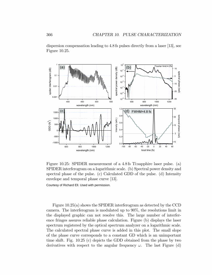
dispersion compensation leading to 4.8 fs pulses directly from a laser [13], seeFigure 10.25.

Figure 10.25: SPIDER measurement of a 4.8 fs Ti:sapphire laser pulse. (a)SPIDER interferogram on a logarithmic scale. (b) Spectral power density andspectral phase of the pulse. (c) Calculated GDD of the pulse. (d) Intensityenvelope and temporal phase curve [13].

Figure 10.25(a) shows the SPIDER interferogram as detected by the CCDcamera. The interferogram is modulated up to 90%, the resolutions limit inthe displayed graphic can not resolve this. The large number of interfer-ence fringes assures reliable phase calculation. Figure (b) displays the laserspectrum registered by the optical spectrum analyzer on a logarithmic scale.The calculated spectral phase curve is added in this plot. The small slopeof the phase curve corresponds to a constant GD which is an unimportanttime shift. Fig. 10.25 (c) depicts the GDD obtained from the phase by twoderivatives with respect to the angular frequency ω. The last Figure (d)

Courtesy of Richard Ell. Used with permission.


shows the intensity envelope with a FWHM pulse duration of 4.8 fs togetherwith the temporal phase curve.

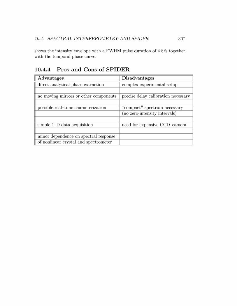
10.4.4 Pros and Cons of SPIDERAdvantages Disadvantagesdirect analytical phase extraction complex experimental setup

no moving mirrors or other components precise delay calibration necessary

possible real—time characterization “compact" spectrum necessary(no zero-intensity intervals)

simple 1—D data acquisition need for expensive CCD—camera

minor dependence on spectral responseof nonlinear crystal and spectrometer

Bibliography

[1] K. Naganuma, K. Mogi, H. Yamada, "General method for ultrashortlight pulse chirp measurement," IEEE J. of Quant. Elec. 25, 1225 -1233 (1989).

[2] J. C. Diels, J. J. Fontaine, and F. Simoni, "Phase Sensitive Measurementof Femtosecond Laser Pulses From a Ring Cavity," in Proceedings of theInternational Conf. on Lasers. 1983, STS Press: McLean, VA, p. 348-355.J. C. Diels et al.,"Control and measurement of Ultrashort Pulse Shapes(in Amplitude and Phase) with Femtosecond Accuracy," Applied Optics24, 1270-82 (1985).

[3] J.W. Nicholson, J.Jasapara, W. Rudolph, F.G. Ometto and A.J. Taylor,"Full-field characterization of femtosecond pulses by spectrum and cross-correlation measurements, "Opt. Lett. 24, 1774 (1999).

[4] D. T. Reid, et al., Opt. Lett. 22, 233-235 (1997).

[5] R. Trebino, "Frequency-Resolved Optical Gating: the Measurement ofUltrashort Laser Pulses,"Kluwer Academic Press, Boston, (2000).

[6] Trebino, et al., Rev. Sci. Instr., 68, 3277 (1997).

[7] Kane and Trebino, Opt. Lett., 18, 823 (1993).

[8] Stark, Image Recovery, Academic Press, 1987.

[9] L. Cohen, "Time-frequency distributions-a review, " Proceedings of theIEEE, 77, 941 - 981 (1989).

369

370 BIBLIOGRAPHY

[10] L. Gallmann, D. H. Sutter, N. Matuschek, G. Steinmeyer and U. Keller,"Characterization of sub-6fs optical pulses with spectral phase inter-ferometry for direct electric-field reconstruction," Opt. Lett. 24, 1314(1999).

[11] C. Iaconis and I. A. Walmsley, Self-Referencing Spectral Interferometryfor Measuring Ultrashort Optical Pulses, IEEE J. of Quant. Elec. 35,501 (1999).

[12] C. Froehly, A. Lacourt, J. C. Vienot, "Notions de reponse impulsionelleet de fonction de tranfert temporelles des pupilles opticques, justifica-tions experimentales et applications," Nouv. Rev. Optique 4, 18 (1973).

[13] Richard Ell, "Sub-Two Cycle Ti:sapphire Laser and Phase SensitiveNonlinear Optics," PhD-Thesis, University of Karlsruhe (TH), (2003).

Chapter 10 Pulse Characterization

Documents

Transcript of Chapter 10 Pulse Characterization