10.1

Chapter 10Journey to Crime Estimation

The J ourney to Crim e (J tc) rout ine is a dis tance-based method which makesest im ates about the likely residen t ia l loca t ion of a ser ia l offender . I t is an applica t ion oflocation th eory, a framework for iden t ifyin g opt im al loca t ion s from a dis t r ibu t ion ofmarket s, supply character is t ics , pr ices, a nd event s. The followin g discussion gives somebackgr ound to the technique. Those wish in g t o skip th is par t can go t o page 10-19 for thespecifics of the J t c rou t ine.

Loca tio n The ory

Loca t ion theory is concerned wit h one of the cent ra l issues in geograph y. Thistheory at t empt s t o find an opt ima l loca t ion for any par t icu lar dist r ibut ion of act ivities,popula t ion, or even t s over a region (Ha gget t , Cliff and F rey, 1977; Kr ueckeberg andSilvers, 1974; Stopher and Meybu rg, 1975; Oppenheim , 1980, Ch . 4; Bossard, 1993). Inclassic loca t ion theory, economic resour ces wer e a lloca ted in r elat ion to idealizedrepr esen ta t ions (Anselin a nd Ma dden , 1990). Thu s, von Thü nen (1826) ana lyzed thedis t r ibu t ion of agr icu lt u ra l land as a funct ion of the accessibilit y t o a sin gle popula t ioncenter (which would be more expensive towards the cen ter ), t he va lu e of the productproduced (which would va ry by cr op), a nd t ranspor ta t ion cost s (which would be moreexpen sive far ther from the cen ter ). In order to ma ximize profit and m in imize cost s, adis t r ibu t ion of agr icu lt u ra l land uses (or crop areas) emerges flowin g ou t from thepopula t ion cen ter as a ser ies of concent r ic r in gs . Weber (1909) ana lyzed the dis t r ibu t ion ofin dust r ia l loca t ion s as a funct ion of the volume of mater ia ls to be sh ipped, t he dis t ancetha t the goods had t o be sh ipped, and t he u n it dis t ance cost of sh ipp ing; consequ en t ly,indust r ies become loca ted in par t icu lar concent r ic zones a round a cen t ra l city. Bur gess(1925) an a lyzed t he dist r ibu t ion of urba n land u ses in Ch icago an d described concent r iczones of both indust r ia l and r es iden t ia l u ses . Their t heory formed the backdrop for ea r lystudies on the ecology of cr im in a l behavior and ga ngs (Th rasher , 1927; Shaw, 1929).

In more modern use, t he loca t ion of persons wit h a cer t a in need or behavior (the‘demand’ side) is iden t ified on a spa t ia l pla ne and p laces a re selected as t o ma ximize valueand m inimize t r avel cost s. F or exa mple, for a consu mer faced with two ret a il sh ops sellingthe sa me pr odu ct , one being closer but more expens ive while the other being fa r ther butless expensive, the consu mer has t o t r ade off the value to be gained a gainst the increa sedt ravel t ime r equ ired. In design ing facilit ies or p laces of a t t r action (th e ‘su pp ly’ side), thedis tance between each possible facilit y loca t ion and the loca t ion of the releva nt popula t ionis compared to the cost of loca t in g n ear the facilit y. For exa mple, given a dis t r ibu t ion ofconsumers and their p ropens ity to spend , such a theory a t t empts to loca te the op t imalplacement of reta il st ores, or , given the dist r ibut ion of pa t ient s, the theory at t empt s t oloca te the opt ima l placemen t of medica l facilit ies.

10.2

Predic t ing Locat ions from a Dis tribut ion

On e can a lso rever se the logic. Given the dist r ibu t ion of demand, t he t heory couldbe a pp lied to est imate a cent ra l loca t ion from which t ravel dist ance or t ime is min imized. On e of the ea r liest uses of th is logic wa s t ha t of J ohn Sn ow, who was in ter ested in thecauses of cholera in t he mid-19th cen tury (Cliff and H agget t , 1988). He postu lat ed t hetheory th a t wa ter was t he major vector t r ansm itt ing the cholera bacter ia. Afterinves t iga t ing water sources in the London met ropolit an a rea and conclud ing tha t there wasa rela t ionsh ip between contamina ted wa ter and choler a cases, he wa s a ble t o confirm histheory by a n outbreak of cholera cases in the Soho dis t r ict . By plot t in g t he dis t r ibu t ion ofthe cases a nd lookin g for wa ter sources in the cen ter of the dist r ibu t ion (essen t ia lly, thecenter of minimum dista nce; see cha pter 4), he foun d a well on Broad St reet t ha t was, infact , cont amina ted by seepage from nea rby sewer s. Th e well was closed a nd t he epidemicin Soho receded. Inciden t ly, in plot t in g t he in ciden t s on a map and look in g for the cen ter ofthe dis t r ibu t ion , Snow applied the same logic t ha t had been followed by t he LondonMet ropolita n Police Depa r tment who had developed t he famous ‘pin’ map in the 1820s.

Theoret ica lly, th ere is an opt ima l solut ion tha t minim izes t he dist ance betweendemand a nd supply (Rush ton, 1979). However , computa t iona lly, it is an a lmost imposs ibletask to define, requ ir ing the en umer a t ion of ever y possible combina t ion . Consequ en t ly inpract ice, a pproximate, t hough sub-opt im al, solu t ion s a re obt a in ed th rough a va r iety ofmethods (Everet t , 1974, Ch . 4).

Trave l Dem an d Modeling

A su b-set of locat ion theory m odels t he t r avel beh avior of individua ls. It actu a lly isthe converse. If loca t ion theory a t t empts to a lloca te pla ces or sit es in rela t ion to bot h asu pp ly-side and dem and-side, t r avel demand t heory a t t em pt s t o model h ow ind ividu a lst ravel between places, given a pa r t icu lar const ellat ion of them. One concept tha t has beenfrequent ly used for th is pu rpose is th a t of the gravity fun ction , a n applica t ion of Newton’sfundamenta l law of a t t r act ion (Oppenheim, 1980). In the or igina l Newton ian formula t ion ,th e att ra ction, F, between t wo bodies of respective masses M 1 an d M 2, sepa ra ted by adist ance D, will be equa l t o

M1 M2

F = g ----------------- (10.1) D2

where g is a const an t or scalin g factor wh ich en su res tha t the equ a t ion is ba lanced inter ms of th e m ea su rem en t un it s (Oppenheim , 1980). As we a ll know, of cour se , g is thegravita t iona l cons tan t in the Newton ian formula t ion . The numera tor of the funct ion is theattraction t erm (or , a lt erna t ively, the a t t r act ion of M2 for M1) wh ile the denomin a tor of theequ a t ion, d 2, indica tes tha t the a t t r act ion between the two bod ies fa lls off as a funct ion oftheir squared d is t ance. It is an im pedance t erm.

10.3

Soc ia l Applications o f the Gravi ty Concept

The gra vity model ha s been the bas is of many app lica t ions t o human societies a ndhas been applied t o social int eract ions sin ce the 19 t h cen tury. Ra venstein (1895) andAndersson (1897) applied the concep t to the ana lys is of migra t ion by a rgu ing tha t thetendency t o migra te between regions is in versely propor t ion a l t o the squared dis t ancebet ween the r egions . Reilly’s ‘law of ret a il gravita t ion’ (1929) applied the Newt onia ngra vity model directly an d su ggest ed t ha t reta il t r avel between two centers would bepropor t ion a l t o the product of their popula t ion s and in versely propor t ion a l t o the square ofthe dist ance sepa ra t ing them:

P i P j

T ij = " ----------------- (10.2) Dij

2

where T ij is th e int eraction between center s i an d j, P i an d P j a re t he r espectivepopula t ions , D ij is th e dista nce between t hem r aised to th e second power an d " is aba lancing cons tan t . In the m odel, t he in it ia l popu la t ion, P i, is called a production while thesecond popu la t ion, P j, is called an attraction .

St ewar t (1950) and Zipf (1949) applied t he concept to a wide var iety of ph enomena(migr a t ion , freigh t t r a ffic, excha nge of informat ion) us ing a sim plified form of the gravityequ a t ion

P i P j

T ij = " ----------------- (10.3) Dij

where the terms are as in equa t ion 10.2 bu t the exponent of dis t ance is only 1. In doin g so,they ba sica lly link ed locat ion theory with t r avel beh avior theory. Given a pa r t icula rpa t t ern of in teract ion for any t ype of goods, service or human act ivit y, an opt im al loca t ionof facilit ies sh ould be solvable.

In t he Stewar t/Zipf fra mework , th e two P’s were both populat ion sizes and,therefore, t heir sums had to be equa l. However , in modern use, it ’s not necessa ry for thepr oductions a nd a t t r actions t o be iden t ical u n it s (e.g., P i cou ld be popu lat ion while P j cou ldbe employmen t ).

The tota l volum e of pr odu ct ions (tr ips) from a single loca t ion , i, is est ima ted bysummin g over a ll des t in a t ion locat ions, j:

T i = K P i G (P j/D ij) (10.4) j

Over time, the concept ha s been genera lized an d applied to ma ny different types oft ravel beha vior . For exam ple, Hu ff (1963) applied t he concept to reta il t r ade betweenzones in an u rban a rea using the genera l form of

10.4

Aj$

T ij = " ----------------- (10.5) Dij

8

where T ij is the number of purchases in loca t ion j by r esiden t s of loca t ion i, Aj is thea t t ractiveness of zone j (e.g., squ are foota ge of ret a il space), D ij is the dist ance betweenzones i an d j, $ is the exponent of S j, and 8 is th e exponent of dista nce, an d " is a cons tan t(Bossard, 1993). Dij

-8 is somet imes ca lled an inverse d istance fun ction. This is a singleconstrain t model in tha t only t he a t t r activen ess of a commer cial zone is const ra ined, tha t isthe sum of a ll a t t r act ion s for j must equa l t he tota l a t t r act ion in the region .

Again , it can be gen er a lized t o all zones by, fir st , est imat ing the t ota l t r ipsgener a ted from one zone, i, t o another zone, j,

P iD Aj

$

T ij = " ----------------- (10.6) Dij

8

where T ij is t he in ter action bet ween two locat ions (or zones), P i is product ions of t r ip s fromloca t ion/zone i, Aj is t he a t t r activeness of locat ion/zone j, Dij is th e dista nce between zones ian d j, $ is the exponent of S j, D is the exponent of H i, 8 is th e exponent of dista nce, an d " isa const an t .

Second, t he t ota l number of t r ips genera ted by a locat ion , i, to a ll des t ina t ions isobt a in ed by summin g over a ll des t in a t ion locat ions, j:

T i = " P iD G (Aj

$/D ij 8) (10.7)

j

Th is differ s from the t r adit ion a l gravity fu nct ion by a llowin g t he exponents of thepr odu ct ion from loca t ion i, the a t t r act ion from loca t ion j, an d t he dist ance between zones t ovar y. Typica lly, th ese exponents a re ca libra ted on a kn own sa mple before being applied t oa forecas t sa mple and t he loca t ions a re u su a lly mea su red by zones. Thus, r et a iler s indecid in g on the loca t ion of a new store can use th is type of model t o choose a sit e loca t ion toopt imize t r avel beh avior of pa t rons ; th ey will, typically, obt a in da ta on a ctu a l sh oppin gt r ips by cu stomers and then ca libra te the model on the da ta , est im at in g t he exponents ofa t t r act ion and dis t ance. Th e model ca n then be used to predict fu ture shoppin g t r ips if afacilit y is bu ilt a t a pa r t icula r loca t ion.

This type of funct ion is ca lled a double const ra in t model because the ba lancingcons tan t , K, has to be cons t ra ined by the number of un it s in both the or igin anddest in a t ion loca t ion s; tha t is , t he sum of P i over a ll loca t ion s must be equa l t o the tota lnumber of product ion s while the sum of P 2 over a ll loca t ion s must be equa l t o the tota lnu mber of at tr actions. Adjust ment s ar e usua lly required to ha ve the sum of individua lproduct ion s and a t t r act ion s equa l t he tota ls (usua lly est im ated in dependent ly).

10.5

The equa t ion can be gener a lized t o other types of t r ips a nd differen t met r ics can besubst it u ted for dis t ance, such as t r avel t im e, effor t , or cost (Isa rd, 1960). F or exa mple, forcommut ing t r ip s, u sua lly employmen t is used for a t t r act ions, fr equen t ly sub-d ivided in toreta il and non-reta il employment . In addit ion , for product ion s, m edia n household in comeor ca r ownersh ip percen tage is used as an add it iona l p roduct ion var iable. Equa t ion 10.7can be genera lized to in clu de any t ype of product ion or a t t r act ion va r ia ble (10.8 and 10.9):

T ij = "1 P iD "2 Aj

$/D ij 8 (10.8)

T i = "1 P iD G ("2 Aj

$/D ij 8) (10.9)

where T ij is t he n umber of t r ips pr oduced by locat ion i t ha t t ravel t o locat ion j, P i is eith er asin gle va r ia ble associa ted wit h t r ips produced from a zon e or the cross-product of two ormore var iables associa ted wit h t r ips pr oduced from a zone, Aj is eit her a sin gle var iableassociat ed with t r ips a t t r acted t o a zone or the cross-produ ct of two or more var iablesassocia ted wit h t r ips a t t r acted t o a zone, D ij is eit her the dis t ance between two loca t ion s oranoth er var iable m ea su r ing t ravel effor t (e.g., tr avel t ime, t r avel cost ), D, $, and 8 a r eexponents of th e r espective ter ms, "1 is a const an t a ssociated with th e productions t oensure tha t the sum of t r ips produced by a ll zon es equa ls the tota l n umber of t r ips for theregion (usu ally estimat ed independent ly), an d "2 is a cons tan t a ssocia ted with thea t t ract ion s to ensure tha t the sum of t r ips a t t r acted to a ll zon es equa ls the tota l n umber oft r ips for the r egion. Without having two cons tan t s in the equ a t ion , usu a lly conflict ingest im ates of K will be obt a in ed by ba la ncin g t he equa t ion aga in st product ion s ora t t r act ions. The summat ion over a ll dest ina t ion loca t ions, j (equa t ion 10.9), produces t hetota l number of t r ips from zone i.

In te rv e n in g Op po rt un it ie s

Stouffer (1940) modified the sim ple gr avity fu nct ion by a rgu in g t ha t the a t t r act ionbet ween two locat ions wa s a fun ction not on ly of the character ist ics of the r ela t ivea t t ractions of two locat ions, bu t of in ter ven ing opport un it ies bet ween the loca t ions. H ishypothesis “..assumes tha t ther e is no necessary rela t ionsh ip bet ween mobility anddis tance... t ha t the number of persons going a given dis t ance is dir ect ly propor t ion a l t o thenumber of oppor tun it ies a t tha t dis t ance and in versely propor t ion a l t o the number ofint ervening opport un ities”(St ouffer , 1940, p. 846). This m odel was u sed in the 1940s toexpla in in ter sta te and in tercounty m igra t ion (Br igh t and Th omas, 1941; Isbell, 1944; Isa rd,1979). Usin g the gravity type form ula t ion , we can wr ite t h is a s:

Aj$

T ji = " ----------------- (10.10) G(Ak

>) D ij 8

where T ji is t he a t t r action of loca t ion j by r es iden t s of locat ion i, Aj is th e att ra ctiveness ofzone j, Ak is the a t t r act iveness of a ll other loca t ions t ha t a re interm ediate in d is tancebet ween loca t ions i and j, D ij is th e dista nce between zones i an d j, $ is the exponent of S j, >is the exponent of Sk , 8 is th e exponent of dista nce, an d " is a cons tan t . While the

10.6

in ter ven ing oppor tun it ies a re im plicit in equ a t ion 10.5 in the exponents, $ an d 8, andcoefficien t , K, equa t ion 10.10 makes the in tervenin g oppor tun it ies explicit . The im por tanceof the concept is tha t the in teract ion between two loca t ion s becomes a complex fu nct ion ofthe spa t ia l environment of nearby a reas and not ju st of the two loca t ion s.

Urban Transp ortation Modeling

This type of model is incorpora t ed as a forma l s tep in the u rban t r anspor t a t ionplanning pr ocess, implemented by most regiona l plan ning organ izat ions in the Un itedSt a tes and elsewh er e (Stopher and Meybu rg, 1975; Kr ueckeber g and Silvers, 1974; Fieldan d MacGregor, 1987). The step, called trip d istribu tion , is lin ked to a five st ep model. F ir st , da ta a re obta ined on t ravel beh avior for a var iet y of tr ip purposes. Th is is usu a llydone by samplin g househ olds and a sk ing each m em ber to keep a t r avel dia ry documen t inga ll their t r ips over a two or th ree da y period. Tr ips a re aggregat ed by individua ls and byhouseholds. F requent ly, t r ips by differen t purposes a re separa ted. Second, t he volume oft r ips pr oduced by and a t t r acted t o zones (ca lled t r a ffic ana lysis zones) is est imated, usu a llyon the basis of the number of households in the zon e and some in dica tor of in come orpr iva te vehicle ownersh ip. Third , tr ips pr odu ced by each zone are dist r ibut ed t o everyother zon e usua lly u sin g a gr avity-t ype funct ion (equa t ion 10.9). Tha t is , t he number oft r ips pr oduced by each or igin zone and endin g in ea ch dest ina t ion zone is est imated by agravity model. The d is t r ibu t ion is based on t r ip product ions , t r ip a t t r act ions , and t ravel‘resist ance’ (measu red by t ravel dis t ance or t r avel t ime). Four th , zone-to-zone t r ips a rea lloca ted by mode of t r avel (car , bus, wa lking, etc); and, fifth , tr ips a re assigned t opa r t icula r rout es by t ravel mode (i.e., bus t r ips follow differ en t rout es than pr ivate veh iclet r ips ). The adva ntage of th is process is tha t t r ips are a llocat ed accord ing to or igins,dest ina t ions, dist ances (or t r avel t imes ), modes of t r avel and r ou tes. Since all zones a remodeled sim ult aneously, a ll in termedia te dest in a t ion s (i.e ., in terven in g oppor tun it ies) areincorpora ted into th e model. Chapt ers 11-17 present a crime tr avel deman d model.

Alternat ive Dis tance De cay Funct ions

One of the pr oblems with the t r adit iona l gravity formulat ion is in t he measu rementof t r avel resist ance, either dist ance or t ime. For loca t ions separa ted by sizeable dist ancesin spa ce, th e gra vity formulat ion can work p roper ly. However , as t he dist ance betweenloca t ions decreases , t he denomina tor approaches in fin ity. Consequen t ly, an a lt erna t iveexpr ession for the in ter action has been pr oposed which u ses t he nega t ive exponen t ia lfunct ion (Hägerst rand, 1957; Wilson, 1970).

Aji = S j$ e (-"Dij) (10.11)

where Aji is t he a t t r action of loca t ion j for res iden t s of locat ion i, S j is th e att ra ctiveness of

loca t ion j, D ij is th e dista nce between locat ions i an d j, $ is the exponent of S j, e is th e base

of the n a tura l logar ithm (i.e., 2.7183...), and " is an empir ica lly-der ived exponent .Somet imes known as entropy m axim ization , th e lat ter pa rt of th e equat ion includes a

nega t ive exponent ia l fun ction wh ich h as a maximum value of 1 (i.e., e -0 = 1). This ha s th e

10.7

adva ntage of makin g t he equa t ion more st able for in teract ion s between loca t ion s tha t a reclose together . For example, Cliff and H agget t (1988) used a nega t ive exponent ia l gravity-type model t o descr ibe the diffusion of measles in to the Un ited St a tes from Canada andMexico. It h as a lso been a rgued t ha t the negat ive exponent ial funct ion gener a lly gives abet t er fit t o urban t ravel pa t t erns, pa r t icu lar ly by au tomobile (Foot , 1981; Bossa rd, 1993;NCH RP , 1995).

Other funct ions h ave also be used t o describe the dist ance decay - negat ive linear ,normal d is t r ibu t ion , logn ormal d is t r ibu t ion , quadra t ic, Pareto funct ion , square rootexponent ial, an d so for th (Hagget t and Arnold, 1965; Taylor , 1970; Eldr idge an d J ones,1991). La ter in the chapter , we will explor e severa l d ifferen t mathemat ica l for mula t ion sfor descr ibin g t he dis t ance decay. One, in fact , does not need to use a mathemat ica lfunct ion a t a ll, bu t cou ld empir ica lly descr ibe the d is tance decay from a la rge da ta set andut ilize th e described va lues for pr edict ions. The u se of mathemat ica l funct ions h as evolvedout of both the Newton ian t rad it ion of gravity as well a s va r ious loca t ion theor ies whichused t he gra vity funct ion . A mathemat ica l funct ion makes sen se u nder two condit ions: 1)if t r avel is un iform in a ll d ir ect ions; and 2) a s an approxima t ion if t here is inadequa te dat afrom which to ca libra te an empir ica l funct ion . The fir s t a ssumpt ion is usua lly wrong s inceph ysica l geogra ph y (i.e., oceans, r ivers, mounta ins ) as well as asymmet r ica l st r eetnet works m ake t ravel ea sier in some direct ions than oth er s. As we sha ll see below, thedist ance decay is quit e irr egula r for journey to cr ime t r ips a nd would be bet t er described byan empir ica l, ra ther than mathemat ica l fu nct ion .

In sh ort , ther e is a long hist ory of resea rch on both the loca t ion of pla ces a s well a sthe likelih ood of int er action bet ween these places, whet her the in ter action is fr eigh tmovement , land pr ices or in dividua l t r avel behavior . The gr avity m odel a nd va r ia t ion s onit have been used to descr ibe the in teract ion s between these loca t ion s.

Trave l Be h av io r of Crim in als

Jou rney to Cr ime Trips

Th e a pp licat ion of tr avel behavior t heory to cr ime h as a sizeable h ist ory a s well. The ana lysis of dis t ance for jour ney to cr ime t r ips wa s a pp lied in the 1930s by White(1932), who noted t ha t pr oper ty cr ime offender s gener a lly t r aveled far ther dist ances t hanoffender s commit t ing cr imes against people, and by Lot t ier (1938), who an a lyzed t he r a t ioof cha in s tore bur gla r ies to the number of cha in s tores by zone in Det roit. Turner (1969)ana lyzed delinqu en cy beh avior by a dis t ance decay t ravel fun ction sh owing h ow more cr imet r ips ten d t o be close to th e offender ’s h ome wit h the frequ en cy dropping off with dis t ance. Ph illips (1980) is, apparen t ly, th e firs t to use t he term journey to crim e is describing thet ravel dist ances t ha t offenders m ake t hough Har r ies (1980) noted t ha t the a ver agedis tance t r aveled has evolved by t ha t t im e in to an ana logy wit h the journey t o workst a t ist ic.

Rh odes and Con ly (1981) expanded on the concep t of a crim inal com m ute andsh owed h ow robbery, bur gla ry an d r ape pa t t erns in the Dist r ict of Colum bia followed a

10.8

dis tance decay pa t t er n . LeBea u (1987a ) an a lyzed t ravel dis t ances of rape offender s in Sa nDiego by vict im-offender relat ionsh ips a nd by met hod of appr oach . Boggs (1965) appliedthe in ter ven ing opport un it ies model in ana lyzing t he dist r ibu t ion of crim es by a rea inrela t ion to th e dist r ibu t ion of offender s. Ot her em pir ical descrip t ions of journey to cr imedis tances and other t r avel behavior parameter s have been studied by Blumin (1973),Cu r t is (1974), Repet to (1974), Pyle (1974), Capone and Nich ols 1975), Renger t (1975),Sm ith (1976), LeBeau (1987b), an d Canter and La rkin (1993). It h as gener a lly beenaccep ted tha t proper ty cr im e t r ips a re lon ger than persona l cr im e t r ips (LeBeau , 1987a),though except ions have been noted (Turner , 1969). Also, it would be expected t ha taverage t r ip dis t ances will va ry by a number of factors: cr im e type; method of opera t ion ;t im e of day; a nd, even , t he va lu e of the proper ty r ea lized (Ca pone and Nich ols , 1975).

Mode lin g th e Offe n de r Se arc h Area

Concept ua l work on t he t ype of model h ave been made by Br an t ingham andBrant ingham (1981) who ana lyzed the geom etry of crim e and concept ua lized a crim ina lsea rch area , a geogra ph ica l ar ea modified by th e spa t ial dist r ibut ion of poten t ial offender sand poten t ia l t a rget s, t he awareness spaces of poten t ia l offenders, a nd the exch ange ofin format ion between poten t ia l offenders . In th is sense, their formula t ion is simila r to tha tof Stouffer (1940), who descr ibed in tervenin g oppor tun it ies, t hough their ’s is a behaviora lfra mework . An import an t concept developed by th e Bra nt ingha m’s is th at of decreasedcr imina l act ivity near to an offender ’s home base, a sor t of a sa fety a rea a round their nearneighborhood. P resumably, offenders, pa r t icu la r ly those commit t in g proper ty cr im es, go alit t le wa y from their home ba se so as t o decrea se the likelih ood t ha t they will get cau ght .Th is was n oted by Turner (1969) in h is s tudy of delin qu en cy in P hiladelph ia . Thus, t heBrant in gh am’s postu la ted tha t there would be a small sa fety a rea (or ‘buffer ’ zon e) ofrelat ively lit t le offender act ivity near to the offender ’s ba se loca t ion ; beyond t ha t zone,however , t hey postu la ted tha t the number of cr im e t r ips would decrease accordin g t o adis tance decay m odel (t he exact mathemat ica l for m was never specified, h owever ).

Cr im e t r ips may n ot even begin a t an offender ’s residence. Rout in e act ivit y t heory(Cohen and F elson , 1979; 1981) su ggest s t ha t cr ime opport unities a ppea r in t he act ivitiesof everyday life. The rout in e pa t t erns of work, shoppin g, and leisure a ffect the convergencein t ime a nd p lace of would be offen ders, su it able t a rget s, a nd a bsen ce of gua rdia ns. Manycr imes may occur while an offender is t r aveling from one act ivity t o another . Thu s,modeling cr ime t r ips as if they a re r eferen ced r ela t ive to a r esidence is not n ecessa r ilygoing t o lead to bet t er predict ion .

Th e m athem at ics of journey t o cr ime h as been modeled by Ren ger t (1981) usin g amodified gener a l opport un it ies model:

P ij = K U i Vj f(D ij) (10.12)

where P ij is the pr obability of an offender in loca t ion (or zone) i committ ing an offense a tloca t ion j, U i is a m easu re of the number of cr ime t r ips pr odu ced a t loca t ion i (wha t Renger tcalled em issiveness), Vj is a measure of the number of crim e ta rget s (a t t r act iveness) a t

10.9

loca t ion j, a nd f(D ij) is a n unspecified fun ction of the cost or effor t expended in t r avelingfrom loca t ion i to loca t ion j (dist ance, time, cost ). He did n ot t ry to oper a t iona lize eith erthe production side or t he a t t r action side. Never theless, concept ua lly, a cr ime t r ip wouldbe expected to involve both elem en ts a s well a s t he cost of the t r ip.

In sh ort , ther e has been a grea t dea l of res ea rch on the t r avel beh avior of crim ina lsin comm itting acts a s well as a nu mber of sta tistical form ulat ions.

P re dic tin g th e Loca tio n of Se rial Offen de rs

The journey to cr ime formulat ion , as in equa t ion 10.9, has been used t o est ima te theorigin locat ion of a ser ia l offen der ba sed on the dist r ibu t ion of crim e inciden t s. Th e logic isto plot the dis t r ibu t ion of the in ciden t s and then use a proper ty of t ha t dis t r ibu t ion toest im ate a likely or igin loca t ion for the offender . Inspect in g a pa t t ern of cr im es for acen t ra l loca t ion is an in tu it ive idea tha t police depar tments have used for a long t ime. Thedis t r ibu t ion of inciden t s describes a n activit y area by an offender , who lives somewh er e inth e center of th e distr ibut ion. It is a sam ple from the offender ’s act ivity space. Using theBrant ingham’s t erminology, th ere is a s earch area by an offender with in wh ich the cr imesare committ ed; most likely, the offender a lso lives with in t he sea rch area .

For example, Canter (1994) shows how the a rea defin ed by the dis t r ibu t ion of the‘J ack the Ripper ’ murders in the east end of Lon don in the 1880s in clu ded the key suspect sin the case (though the case was never solved). Kin d (1987) ana lyzed the in ciden t loca t ion sof th e ‘York shire Ripper’ who comm itted th irteen mu rders a nd seven at tem pted mu rders innor theast England in the lat e 1970s and ea r ly 1980s. Kind a pplied t wo differen tgeograph ical cr it er ia to est imate t he r es iden t ia l loca t ion of th e offender . Fir st , heest im ated the cen ter of min im um dis tance. Second, on the assumpt ion tha t the loca t ion s ofthe murders and a t t empted murders tha t were commit ted la te a t n igh t were closer to theoffender ’s residence, h e gr aphed the t im e of the offense on the Y axis aga in st the month ofthe yea r (ta ken as a pr oxy for length of da y) on the X axis and p lott ed a t r en d lin e t h roughthe da ta to account for sea sona lity. Both the cen ter of minim um dist ance and t he murder scommit ted a t a la ter t ime than the t r end line poin ted towards the Leeds/Bradford a rea ,very close to wh ere the offen der actua lly lived (in Br adford).

R os sm o Mo de l

Rossmo (1993; 1995) has adapted loca t ion theory, pa r t icu la r ly t r avel behaviormodeling, to ser ia l offenders. In a ser ies of papers (Rossmo, 1993a ; 1993b; 1995; 1997) heout lined a mathem at ical a pproach to iden t ifying the home base locat ion of a ser ia loffender , given the d is t ribu t ion of t he inciden t s. The ma themat ics rep resen t a formula t ionof the Bran t ingham and Bran t ingham (1981) sea rch a rea model, d iscussed above in whichthe sea rch behavior of an offender is seen as followin g a dis t ance decay function wit hdecreased act ivit y n ear the offender ’s home base. H e has produced exa mples showin g h owthe model ca n be applied to ser ia l offenders (Rossmo, 1993a ; 1993b; 1997).

10.10

The model ha s four steps (what he called crim ina l geographic targeting):

1. F ir st , a rectangu la r study a rea is defin ed tha t extends beyon d the a rea of theinciden t s committ ed by th e ser ial offender . The avera ge dista nce betweenpoin t s is t aken in both the Y and X dir ect ion . H a lf t he Y in ter -poin t dis t anceis a dded to th e m aximum Y value and subt racted from t he m inimum Yvalue. Ha lf the X in ter -poin t d is tance is added to the maximum X va lue andsu bt racted from t he minim um X value. These a re bas ed on pr ojectedcoordina tes; presum ably, th e directions would have to be adjusted ifspher ica l coor din a tes were used. The rectangu la r study defin es a gr id fromwhich column s an d rows can be defined.

2. For each grid cell, the Manha t tan dist ance to each inciden t loca t ion is taken(see chapter 3 for defin it ion ).

3. For ea ch Man ha t tan distance from a gr id cell to an incident loca t ion , MDij,one of two funct ions is evalu a ted:

A. If the Man ha t tan distance, MD ij, is less than a specified buffer zon eradius, B, then

TP ij = A {k[ (1-N)(Bg-f) / (2B - | xi - xc| + | yi - yc| )g] } (10.13) c=1

where P ij is t he r esu ltan t of offender in ter action for gr id cell, i; c is t hein ciden t number , summin g t o T; N = 0; k is a n empir ica lly det erminedcons tan t ; g is an empir ica lly determined exponen t ; and f is anempir ica lly det ermined exponent .

Th e Gr eek let t er , A, is the product sign , indica t in g t ha t the resu lt s foreach grid cell-inciden t distance, MD ij, a r e m ultiplied together acrossall incidents, c. This equa tion r educes to

TP ij = A {k(1-0)(Bg-f) / (2B - | xi - xc| + | yi - yc| )g } (10.14) c=1

T KBg-f

P ij = A ---------------------------------- (10.15) c=1 (2B - | xi - xc| + | yi - yc| )g

Within the buffer region, the funct ion is the ra t io of a constant , k ,t im es the radiu s of the bu ffer , B, r a ised to another constan t (g-f),

10.11

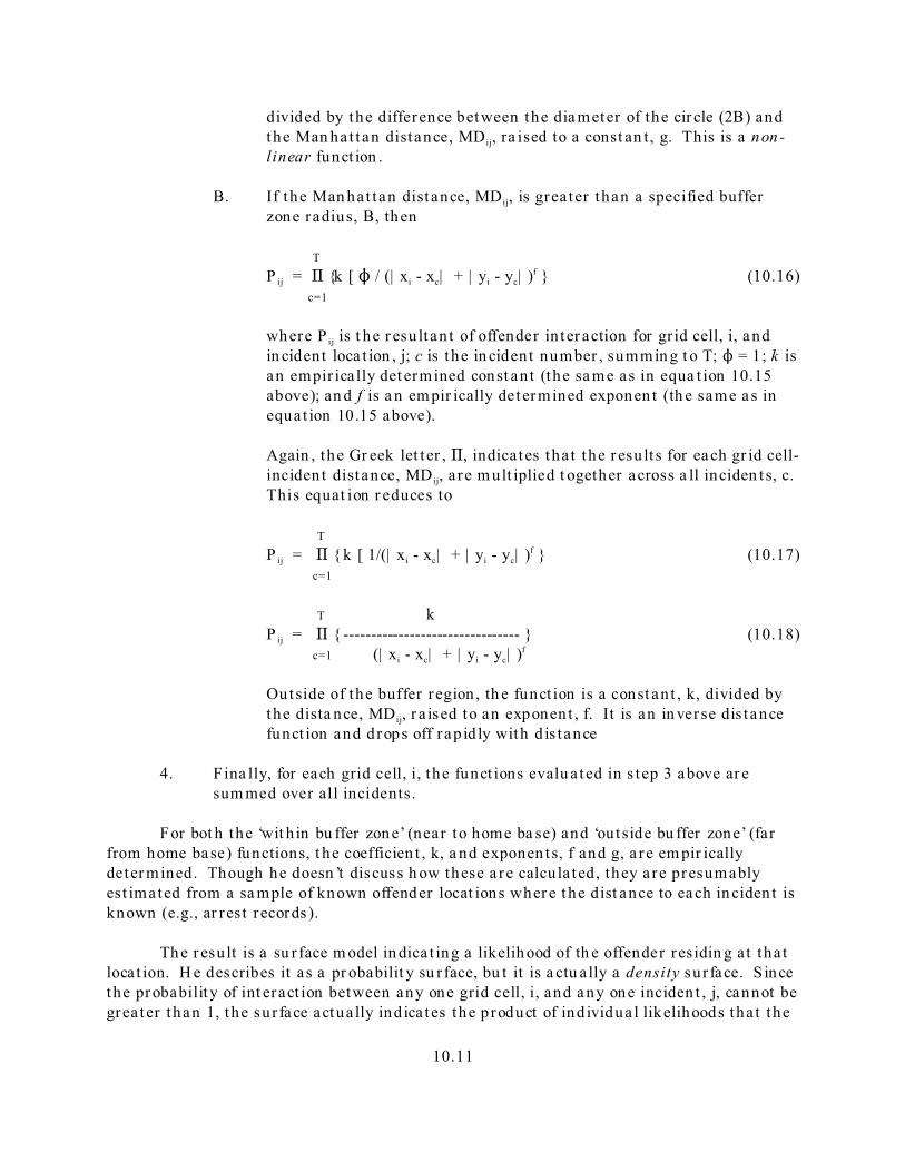
divided by the difference between the dia meter of the cir cle (2B) andthe Man ha t tan distance, MD ij, ra ised to a const an t, g. This is a non-linear funct ion .

B. If the Man ha t tan distance, MD ij, is grea ter than a specified bufferzone radius, B, then

TP ij = A {k [ N / (| xi - xc| + | yi - yc| )f } (10.16) c=1

where P ij is t he r esu lt an t of offender in ter action for gr id cell, i, andin ciden t loca t ion , j; c is the in ciden t number , summin g t o T; N = 1; k isan empir ica lly det ermined const an t (the sa me as in equa t ion 10.15above); an d f is a n em pir ically deter mined exponen t (th e same a s inequa t ion 10.15 above).

Again , the Gr eek let t er , A, indicates tha t the r esu lt s for each gr id cell-inciden t distance, MD ij, a re m ult iplied t ogether across a ll inciden t s, c. This equat ion r educes to

TP ij = A { k [ 1/(| xi - xc| + | yi - yc| )f } (10.17) c=1

T kP ij = A { -------------------------------- } (10.18) c=1 (| xi - xc| + | yi - yc| )f

Outside of the buffer region , th e funct ion is a const an t , k, divided bythe dista nce, MD ij, r a ised to an exponent , f. It is an in verse dis t ancefunct ion and d rops off r ap id ly with d is tance

4. F ina lly, for each grid cell, i, the funct ions evalu a ted in s t ep 3 above ar esum med over all incidents.

For bot h the ‘wit h in bu ffer zon e’ (near to home ba se) and ‘out side bu ffer zon e’ (farfrom home base) functions, t he coefficien t , k, a nd exponen ts, f and g, a re em pir icallydeter mined. Though he doesn ’t discuss h ow these a re calcula ted, they a re presumablyest imated from a sa mple of known offender locat ions wher e t he dist ance to ea ch in ciden t isknown (e.g., ar res t records ).

Th e r esu lt is a su r face m odel in dica t ing a likelih ood of th e offender res idin g a t tha tloca t ion. H e describes it as a pr obabilit y su r face, bu t it is a ctu a lly a density su r face. S incethe pr obability of int eract ion between any one grid cell, i, and a ny one inciden t , j, cannot begrea ter than 1, the su r face actua lly ind ica tes the p roduct of ind ividua l likelihoods tha t the

10.12

offender uses t ha t locat ion as t he home base. To be a n actu a l pr obability function, it wouldhave to be re-sca led so tha t the su m of the grid cells was equa l to 1.

The second function - ‘out side t he bu ffer zone’ (equa t ion 10.16) is a class ic gravityfunct ion , s imila r to equa t ion 10.5 excep t there is no a t t r act ion defin it ion . It is the d is tancedecay par t of the gravity function. The firs t fun ction, equ a t ion 10.13, is an increasin gcurvilinea r funct ion designed to model the area of decrea sed a ct ivity near the offender ’shome bas e.

S tr en gt h s a n d w ea k n esses of th e Ros sm o m od el

The Rossmo model h as both st rengt hs and weaknesses. F ir st , t he model h as sometheoret ica l basis u t ilizin g t he Br an t in gh am and Br an t in gh am (1981) framework for anoffender sear ch ar ea a s well as the ma themat ics of the gravity model an d dist inguish es twotypes of t r avel beha vior - near to home and far ther from home. Second, th e model doesrepresen t a sys temat ic a pproach towards iden t ifyin g a likely home base loca t ion for anoffender . By eva lua t ing each gr id cell in the s tudy a rea , an independen t es t imate of thelikelihood is obta ined, wh ich can then be in tegra ted in to a cont inuous su r face wit h anint erpola t ion gra ph ics r ou t ine.

Th er e a re problems with the par t icula r formula t ion, h owever . Fir st , the exclusiveuse of Manha t tan dis t ances is quest ion able. Unless the study a rea has a st reet networktha t follows a un iform grid, measu r ing dist ances h or izonta lly and vert ica lly can lead tooveres t ima t ion of t r avel d is t ances ; fu r ther , t he more the layou t differ s from a nor th -sou thand east -west orien ta t ion, t he gr ea ter the dist ort ion. S ince many urba n area s do not havea un iform grid st reet layout , th e method will necessa r ily lead to overes t ima t ion of t r aveldista nces in places where there ar e diagona l or irr egular str eets.1

Second, t he u se of a pr oduct t er m, A, complica tes the mathemat ics . Tha t is , thetechnique eva lua tes t he dist ance from a pa r t icu lar grid cell, i, to a pa r t icu lar inciden tloca t ion , j. It t hen m ultiplies th is result by all oth er results. Since the P values areactua lly den sit ies, which can be grea ter than 1.0, the pr ocess, if st r ict ly applied, would be acompoun ding of pr obabilit ies with overes t ima t ion of the likelihood for grid cells close t oinciden t loca t ions and underes t imat ion of the likelihood for gr id cells fa r ther away. In thedescript ion of the method, however, Rossm o actua lly ment ions su mming the terms. Thu s,the subst itu t ion of a summat ion s ign , G, for t he product sign would help th e mat hema tics.

A th ir d problem is in the dis t ance decay fu nct ion (equa t ion 10.16). The use of aninver se dis t ance ter m has p roblems a s t he dist ance bet ween the gr id cell loca t ion, i, a ndthe inciden t loca t ion , j, decreases. For some t ypes of cr imes , th ere will be lit t le or no bufferzone aroun d t he offender ’s h ome ba se (e.g., ra pes by acqua in tances). Consequ en t ly, thebuffer zon e radiu s, B, would approach 0. H owever , t h is would cause the model t o becomeunst able s ince the inver se dis t ance ter m will a pp roach infinit y.

Four th , the u se of a mathem at ical function to descr ibe t he dist ance decay, whileeasy t o defin e, probably oversim plifies actua l t r avel behavior . A m athemat ica l fu nct ion to

10.13

describe dist ance decay is an appr oximat ion to actua l tr avel beha vior . It a ssu mes t ha tt ravel is equa lly likely in each direction , tha t t r avel dis t ance is un iformly easy (or difficult )in each dir ect ion , a nd tha t , s im ila r ly, oppor tun it ies a re un ifor mly dis t r ibu ted. F or mosturban areas, these condit ions would not be tr ue. Few cit ies form a per fect grid (Salt Lak eCit y is, of cou rse, a n except ion ), t hough most cit ies have sect ion s tha t a re gr ided. Bothph ysica l geogra ph y limit t r avel in cert a in d irections a s does the h istor ica l st r eet st ructure,which is often der ived from ear lier communit ies. A m athemat ica l fu nct ion does notconsider th is str uctu re, but ra th er assu mes th at th e ‘impedance’ in a ll directions isun iform.

This la t t er cr it icism, of cou rse, would be t rue for a ll mathemat ica l for mula t ion s oft ravel dis t ance. There a re cor rections t ha t can be m ade to adjus t for th is. F or exa mple, inthe u rba n t ravel dem and t ype model, t r ip d ist r ibu t ion bet ween loca t ions is est imated by agr avity m odel, bu t then the dis t r ibu ted t r ips a re const ra in ed by, fir st , t he tota l n umber oft r ips in the r egion (est imated sepa ra tely), second , by mode of t r avel (bus v. s ingle dr iver v.dr ivers plu s passengers v. wa lk , et c.), and, t h ir d, by t he route st ructure upon which thet r ips a re event ua lly assigned (Kru eckeber g an d Silvers, 1974; St oph er and Meybur g, 1975;Field an d Ma cGregor , 1987). Calibra t ion a t a ll st ages aga ins t kn own da ta set s en su restha t the coefficien t s a nd exponen ts fit ‘r ea l world ’ da ta as closely as possible. It would takethese t ypes of modifica t ions t o make t he t r avel dist r ibut ion type of model post u lat ed byRossmo and others be more rea list ic.

Fifth , th e model imposes m athemat ica l rigidity on the da ta . While th ere a re twodifferen t funct ions tha t cou ld vary from p lace to p lace, the pa r t icu la r type of d is tance decayfunct ion migh t a lso va ry. Specifying a s t r ict form for the two equa t ions limit s theflexibilit y of a pplyin g t he model t o differen t types of cr im e or to pla ces where the dis t ancedecay does not follow the form specified by Rossmo.

A sixth problem is tha t opport un ities for comm itting crimes - th e att ra ctiveness ofloca t ions , a re never measured . Tha t is , there is no enumera t ion of the oppor tun it ies tha twould exis t for an offender nor is there an a t t empt to measure the s t rength of th isa t t r act ion . Ins tead, th e sea rch area is inferr ed st r ict ly from the dist r ibut ion of inciden t s.Because t he dist r ibut ion of offender opport unities would be expected t o var y from place topla ce, t he model would need to be re-ca libra ted a t each loca t ion . In th is sense, both theCanter model and m y journey to cr ime m odel (both descr ibed below) also share t h isweakn ess. It is un der st anda ble in tha t vict im/ta rget oppor tun ities a re difficu lt t o define apriori sin ce they ca n be in terpreted differen t ly by individua ls . Never theless, a morecomplete theory of jou rney t o cr im e behavior would have to in corpora te some measure ofoppor tun it ies , a poin t t ha t both Bran t ingham and Bran t ingham (1981) and Renger t (1981)have ma de.

F in a lly, the ‘buffer zon e’ concep t is bu t one in terpreta t ion of the tendency of manycr imes not to be commit ted close to the home loca t ion . There a re other in terp reta t ions tha ta re applicable. F or exa mple, t he dis t r ibu t ion of cr im e oppor tun it ies is often not close to thehome locat ion , either . Many cr imes occur in commer cial a rea s. In most Amer ican cit ies,residen t ial a reas a re not loca ted in commercial a reas. Thu s, there will usu a lly be a

10.14

dis tance between a residen t ia l loca t ion and a nearby cr im e oppor tun it y. Th is does notimply anyth ing about a ‘sa fety zone’ for the offender bu t , ins tead , may illus t ra te thedis t r ibu t ion of the oppor tun it ies. If we could m ap t he t r avel dis t ance of, sa y, sh oppin gt r ips , we would probably find a sim ilar dis t r ibu t ion to th a t seen in most of journey to cr imest udies (and illu st ra ted below).

The concept of a ‘bu ffer zone’ is a hypothesis, n ot a cert a in ty. The language of it isso appea ling t ha t many people believe it to be t rue. But , t o demonst ra te the exis tence of a‘buffer zone’ would require in terviewing offender s (or offender s wh o have been a r rest ed)and dem onst ra t ing tha t they did not commit crim es n ear their r esiden ce even t hough t herewere opport un ities (i.e., th ey va lued sa fety over oppor tun ity). To my knowledge, there hasnot been a st udy tha t dem onst ra ted t h is yet. Otherwise, one cannot dist ingu ish betweenthe ‘buffer zone’ hypothesis a nd t he dist r ibut ion of available opport un ities. They ma y verywell be t he same t h ing.

Ca n te r Mo de l

Canter ’s group in Liverpool (Canter and Tagg, 1975; Can ter and La rkin , 1993;Canter and Snook, 1999; Ca nter , Coffey a nd Hunt ley, 2000) have modified the dis t ancedecay fu nct ion for journey t o cr im e t r ips by u sin g a nega t ive exponent ia l t erm, instead ofthe inver se dis t ance. Their Dragn et progr am uses the nega t ive exponent ia l fu nct ion

Y = " e (-$ Dij/ P) (10.19)

wh er e Y is the likelih ood of an offender t r avelin g a certa in dis t ance to comm it a crim e,, D ij

is t he dist ance (from a home ba se loca t ion t o an inciden t sit e), " is a n a rbit ra ry const an t , $

is the coefficien t of the dis t ance (a nd, h ence, an exponent of e), P is a normaliza t ion

const an t, and e is t he ba se of the n a tura l logar ithm. The model is similar to equa t ion 10.11

except , lik e Rossmo, it does not in clu de the a t t r act iveness of the loca t ion .

Us ing the logic tha t most cr imes a re committ ed n ear the offender ’s h ome bas e,Ca nter , Coffey and H unt ley (2000) use a five st ep pr ocess t o est imate a sea rch s t ra tegy:

1. The st udy ar ea is defined by a r ectangle tha t is 20% lar ger in a rea than tha tdefin ed by t he min im um and maximum X/Y poin t s. A gr id cell st ructure of13, 300 cells is im posed over the rectangle. E ach gr id cell is a referencelocat ion , i.

2. A decay coefficient is selected. In equa t ion 10.19, th is would be th e

coefficien t , $, for the dist ance ter m, D ij, both of wh ich are exponents of e .

Un like Rossm o, Can ter uses a ser ies of decay coefficient s from 0.1 to 10 toest im ate the sensit ivit y of t he model. The equa t ion in dica tes the likelihoodwit h which any loca t ion is likely to be the home base of the offender based onone inciden t .

10.15

3. Because d ifferen t offender s have d ifferen t sea rch a reas, t he measu reddis tances for each cell a re divided by a norm aliza t ion coefficien t , P , tha tadjus t s a ll offenses t o a compa rable ra nge. Can ter uses t wo differen t typesof normaliza t ion funct ion : 1) mean int er -poin t dist ance between a ll offenses(across a group of offenders ); and 2) the QRange, which is an index tha tt akes int o account asymmet ry in the or ient a t ion of the inciden t s.

4. For each reference cell, i, t he dis t ance between each gr id cell and eachincident locat ion is evalua ted with th e fun ction a nd t he sta nda rdizedlikelihoods a re summed to yield a n est imate of locat ion poten t ia l.

5. A search cost index is defined by the pr oport ion of the st udy ar ea tha t has t obe sear ched to find t he offender. By ca libra t ing th e model agains t kn owncases, an est ima te of sea rch efficiency is obta ined .

Addit iona l mod ifica t ions can be added to the funct ions to make them more flexible(Can ter , Coffey and Hun t ley, 2000). For example, ‘s t eps’ a r e d is t ances nea r t o home whereoffender s a re not likely to act wh ile ‘p la t eaus’ a r e const an t dis t ances nea r t o home wherethere is the h ighest likelihood of act in g. For exa mple, Canter and Larkin (1993) found anarea a round ser ial offender s’ homes of about 0.61 mile in radius with in wh ich they wereless likely to comm it crimes.

Ca nter and Snook (1999) pr ovide es t imates of the sea rch cost (or efficiency)associat ed with var ious dist ance coefficient s. For example, with the kn own home bas eloca t ions of 32 burgla r s, a $ of 1.0 yielded a m ean sea rch cost of 18.06%; tha t is, on avera ge,only 18.06% of th e study a rea had t o be sea rched to find t he loca t ion of 32 bu rglar s in theca libra t ion sample. Clear ly, for some of them, a la rger a rea had to be searched while forothers a smaller a rea ; the average was 18.06%. Conversely, t he mean search cost in dex for24 r apis t s was 21.10% and for 37 m urderer s 28.28%. They fur ther explored the m argina lincrease in loca t ing offender s by increasing the percen tage of t he s tudy a rea tha t had to besea rched. They found for their t h ree sa mples (burgla ry, rape, homicide) th a t more thanha lf the offender s could be loca ted with in 15% of the area sea rched.

The Ca nter model is differen t from the Rossmo model is tha t it suggest s a sea rchst ra tegy by t he police for a ser ia l offender ra ther than a pa r t icula r loca t ion. Th e st ren gthof it is to indica t e how na r row an a rea the police shou ld concen t r a t e on in order t o op timizefind ing an offender . Clea r ly, in most cases , only a sm all a rea needs be sea rched.

S tr en gt h s a n d w ea k n esses of th e Ca n ter m od el

The model h as both st rengt hs and weaknesses. F ir st , t he model provides a sea rchst ra tegy for law en forcemen t . By exa min ing wh at type of fun ction bes t fits a cert a in typeof cr ime, police can ta rget t heir search effor t s m ore efficient ly. The m odel is rela t ively easyto implemen t and is pr act ica l. Second, th e mathemat ica l formulat ion is st able. Un like theinver se dist ance funct ion in t he Rossm o model, equa t ion 10.19 will not have problemsassocia ted wit h dis t ances tha t a re close to 0. Fur ther , t he model does provide a sea rch

10.16

st ra tegy for ident ifying an offender . It is a useful tool for law en forcement officers,pa r t icu lar ly as t hey frame a sea rch for a ser ial offender .

There are a lso weakn esses to the model. First , it lacks a theoret ica l bas is. Can ter ’sresea rch h as p rovided a grea t dea l in ter ms of underst andin g the activit y spaces of ser ia loffender s (Can ter and La rkin , 1993; Can ter and Gr egory, 1994; Can ter , 1994; Hodge an dCanter , 2000). H owever , t he empir ica l m odel u sed is st r ict ly pragm at ic. Second,mathemat ica lly, it imposes t he negat ive exponent ial funct ion with out consider ing otherdist ance decay models. In t he Dragn et pr ogra m, th e decay funct ion is a s t r ing of 20number s so th a t , in theory, a ny function can be explored. However , the defau lt is anega t ive exponent ia l. The nega t ive exponent ia l h as been used in many t ravel behaviorstudies (Foot , 1981; Bossard, 1993), bu t it does not a lways produce the best fit . La ter on,I’ll sh ow exam ples of t r avel beha vior which sh ow a dist inctly non-monotonic funct ion , evenbeyond a home bas e ‘buffer zone’. While the model can be adapt ed t o be more flexible bydifferen t exponents and in clu din g s teps and pla teaus, for exa mple, it is st ill t ied to thenega t ive exponen t ia l form . Thus, t he m odel might work in some loca t ions, bu t may fa il inothers ; a u ser can’t eas ily adjust the model to make it fit n ew da ta .

Th ird, t he coefficien t of the n ega t ive exponent ia l, ", is defined ar bitr ar ily. In t heDragn et pr ogra m, it is usua lly set as 0.5. While th is ensu res t ha t the resu lt n ever exceed1.0 for any one inciden t , there is a limit on the loca t ion poten t ia l summat ion s ince the tota lpoten t ia l is a fun ction of the n umber of inciden t s (i.e., it will be h igher for more inciden t s). Thus, the use of " ends u p being a rbitr a ry. It would have been bet t er if the coefficientwere ca libra ted a gainst a kn own sa mple.

Four th , a nd fin a lly, a lso sim ila r to the Rossmo model (a nd to my J tc model below),cr imina l oppor tun it ies (or a t t r act ions ) a re never measured , bu t a re in fer red from thepa t t er n of crim e inciden t s. As a pr agmat ic tool for in forming a police sea rch, one couldargue t ha t th is is not im port an t . However , in a differen t loca t ion , th e dist ance coefficientis liable to differ as is t he sea rch cost index. It would need t o be re-ca libra ted ea ch t ime.

Never theless, t he Ca nter model is a useful t ool for police depar tmen t and can helpshape a sea rch st ra tegy. I t is differen t from the other loca t ion models in tha t it is notfocused so much on the bes t p red ict ion for a loca t ion of an offender (though the summat iondiscussed a bove in st ep 4 can yield tha t ) as it does in defin ing where the sea rch sh ould beoptimized.

Ge o gra ph ic P ro fi li ng

J ourney t o cr im e est im at ion should be dis t in gu ished from geographical profiling. Geograph ical profiling involves u nderst andin g the geogra ph ical sea rch pa t t er n of crim ina lsin rela t ion to the spa t ia l d is t r ibu t ion of poten t ia l offenders and poten t ia l t a rget s , theawa ren ess spa ces of poten t ia l offen ders in cluding the labelin g of ‘good’ ta rget s a nd cr imeareas, a nd the in terchange of in format ion between poten t ia l offenders who may m odifytheir awareness space (Br an t in gh am and Br an t in gh am, 1981). Accordin g t o Rossmo:

10.17

“...Geogra ph ic pr ofiling focuses on t he pr obable spa t ial behaviour of the offenderwith in the con text of the loca t ions of, and the spa t ia l r ela t ionsh ips between , thevar ious crime sites. A psychologica l profile pr ovides in sight s in to an offender ’slikely mot iva t ion , beha viour and lifest yle, an d is t herefore direct ly connected t oh is/her spa t ial act ivity. Psychologica l an d geogra ph ic pr ofiles th us a ct in t andem tohelp invest igators develop a picture of the per son responsible for the crim es inqu est ion” (Rossmo, 1997).

In other words , geogra ph ic profiling is a framework for un der st anding how anoffender t r averses a n a rea in sea rch ing for vict ims or t a rgets ; th is, of necessit y, involvesunder st anding th e social environment of an a rea , th e way th a t the offender under st andsth is environment (the ‘cognit ive map’) as well as the offender ’s m ot ives.

On the oth er hand, journey to cr ime es t imat ion follows a much s impler logicin volving t he dis t ance dim ension of the spa t ia l pa t t ern in g of a cr im in a l. It is a methoda imed a t est ima t ing the dist ance tha t ser ial offender s will t r avel to commit a cr ime a nd, byimplicat ion, the likely locat ion from which t hey star ted th eir crime ‘tr ip’. In short, it is ast r ict ly st a t ist ica l appr oach to est ima t ing the residen t ial whereabouts of an offendercompa red to un dersta nding the dyna mics of serial offenders.

It remain s an empir ica l quest ion whether a conceptua l fr amework, such asgeographic profiling, can predict bet ter than a s t r ict ly s ta t is t ica l framework. Underst andin g of a phen omena , su ch a s ser ia l murders, ser ia l rapis t s, a nd so fort h , is a nimpor tan t r esea rch a rea . We seek more than jus t st a t is t ica l p red ict ion in bu ild ing akn owledge base. H owever, it doesn ’t necessa r ily follow tha t under st anding produces bet t erpr edictions. In many area s of human activit y, st r ictly st a t ist ical m odels a re bet t er inpredict in g t han expla na tory m odels . I will r etu rn to th is poin t la t er in the sect ion .

Th e Cr i m eS t a t J o u rn e y to Crim e Ro u tin e

The journey to cr ime (J t c) rou t ine is a diagnost ic designed to a id police depa r tmentsin their in vest iga t ion s of ser ia l offenders. The a im is to est im ate the likelihood tha t aser ial offender lives at any par t icu lar loca t ion . Using th e loca t ion of inciden t s committ edby the ser ia l offen der , the program makes st a t ist ical guesses a t wh er e t he offender is lia bleto live, based on the sim ila r it y in t r avel pa t t erns to a known sample of ser ia l offenders forthe sa me type of cr ime. The J tc rou t ine bu ilds on the Rossm o (1993a; 1993b; 1995)fra mework , bu t ext en ds it s m odelin g capabilit y.

1. A grid is over laid on t op of the st udy ar ea . This grid can be eith er impor tedor can be gener a ted by Crim eS tat (see cha pter 2). The grid represents t heen t ire study a rea . Un like Rossmo or Canter and Snook, ther e is n o opt imalst udy ar ea . The t echnique will model tha t which is defined. Thu s, the userhas t o select an a rea in telligen t ly.

2. The rout in e ca lcu la tes the dis t ance between each in ciden t loca t ioncommit ted by a ser ia l offender (or gr oup of offenders workin g t ogether ) and

10.18

each cell, defined by th e cen t roid of the cell. Rossm o (1993a; 1995) usedindir ect (Manha t tan) dist ances. However , th is would be a ppropr ia te onlywhen a city fa lls on a un iform grid. The J tc rou t ine a llows both d irect andin dir ect dis t ances. In most cases, d ir ect dis t ances would be the mostappropr ia te choice a s a police depar tmen t would norm ally locat e origin anddest ina t ion loca t ions r a ther than pa r t icu lar rou tes t ha t a re taken (seebelow).

3. A d is t ance decay funct ion is applied to each gr id cell-inciden t pa ir and sumsthe va lues over a ll inciden t s. Th e u ser has a choice wh et her to model t het ravel dist ance by a m athemat ica l funct ion or an empir ica lly-der ivedfunct ion .

4. The r esu ltan t of the dist ance decay function for each gr id cell-inciden t pa ira re summed over a ll inciden ts t o produce a lik elihood (or densit y) est imatefor ea ch gr id cell.

5. In both cases, t he progr am output s the two resu lt s: 1) the gr id cell which hasthe pea k likelih ood est imate; and 2) th e likelih ood est imate for ever y cell. The la t t er ou tpu t can be saved as a S urfer® for Windows ‘dat ’, ArcViewS pat ial Analyst© ‘asc’, ASCII ‘grd’, ArcView ® ‘.sh p’, MapIn fo® ‘.m if’ ,Atlas*GIS ™ ‘.bn a’ file or as a n Ascii grid ‘grd’ file wh ich can be r ea d by manyGIS packa ges (e.g., AR C/ IN FO®, Vertical Mapper©). These files can a lso berea d by oth er GIS packa ges (e.g., Mapt itude).

F igure 10.1 shows t he logic of the r out ine a nd figure 10.2 shows t he J our ney t oCrime (J tc) screen. There ar e two par ts t o th e rout ine. First, th ere is a calibrat ion m odelwh ich is used in the em pir ically-der ived dis t ance function . Second, t her e is the J our ney t oCr ime (J tc) model it self in which the user can select either the a lready-ca libra ted dis tancefun ction or t he m athem at ical function . The em pir ically-der ived fun ction is, by far , theea siest to use and is , consequ en t ly, th e defau lt choice in Crim eS tat. The discuss ion of it ison p. 35. However , t he ma themat ica l funct ion can be used if t here is inadequa te dat a t oconst ru ct a n empirical dista nce decay fun ction or if a pa rt icular form is desired.

D is ta n ce Mo de lin g Us in g Ma th e m at ic al F u n ct io n s

We’ll s t a r t by illus t ra t ing the use of the mathemat ica l funct ions because th is hasbeen the t r adit iona l way tha t dist ance decay ha s been exam ined. The Crim eS tat J t crout ine a llows t he u ser to define dist ance decay by a mathem at ical function .

P r ob ab ili ty Di st an c e Fu n c ti on s

The user selects one of five probabilit y densit y d is t r ibu t ion s to defin e a likelihoodtha t the offender has t r aveled a par t icu la r dis t ance to commit a cr im e. The adva ntage ofhaving five fun ctions, a s opposed to on ly one, is t ha t it pr ovides m ore flexibility indescr ibing t ravel beh avior . The t ravel dis t ance dist r ibu t ion followed will vary by cr imetype, t im e of day, method of

Journey to Crime Interpolation Routine

Primary file:Crime locations

Reference grid

Travel demand function

Figure 10.1:

Journey to Crime ScreenFigure 10.2:

10.21

opera t ion , and numerous other va r iables . The five funct ions a llow an approach tha t cansimulat e more accura tely t r avel beha vior under differen t condit ions. Ea ch of these h asparameter s tha t can be modified, a llowin g a very la rge number of possibilit ies fordescr ibin g t ravel behavior of a cr imina l.

Figur e 10.3 illust ra tes th e five types.2 Defau lt va lu es based on Ba lt im ore Cou ntyhave been pr ovided for each . The user , however , can change th ese a s n eeded.

Br iefly, th e five funct ions a re:

Li n ea r

The simplest type of dist ance model is a linear funct ion . This m odel post u lat es t ha tthe likelihood of commit t in g a cr im e a t any par t icu la r loca t ion declines by a constan tamount with dist ance from the offender ’s h ome. It is h ighest near the offender ’s h ome butdrops off by a constan t amount for each un it of dis t ance un t il it fa lls to zero. The form ofth e linear equat ion is:

f(d ij) = A +B*d ij (10.20)

where f(d i j) is the likelihood tha t the offender will com mit a cr im e a t a par t icu la r loca t ion ,i, defined h er e a s t he cen ter of a gr id cell, d i j is the dist ance between the offender ’sres idence and loca t ion i, A is a slope coefficien t wh ich defines the fall off in d ist ance, and Bis a const an t . It would be expected t ha t the coefficient B would have a nega t ive sign sin cethe likelihood should decline wit h dis t ance. The user must provide va lu es for A an d B . The defau lt for A is 1.9 and for B is -0.06. This funct ion assumes no bu ffer zon e around theoffender ’s r esidence. When the fun ction rea ches 0 (th e X axis), th e r out ine au toma t icallysubst it u tes a 0 for the funct ion .

Nega t i ve Exponen t ia l

A sligh t ly more complex fun ction is t he nega t ive exponen t ia l. In th is t ype of model,the likelih ood is a lso h ighest nea r the offenders h ome and d rops off with dis t ance. However, the decline is at a const an t rate of decline, thus dr oppin g quickly nea r theoffender ’s h ome unt il is a pp roaches zer o likelihood. The m athem at ical form of the n ega t iveexponen t ia l is

-B*d ijf(d ij) = A*e (10.21)

where f(d ij) is t he likelihood t ha t the offender will commit a crim e a t a pa r t icula r locat ion , i,defined h er e a s t he cen ter of a gr id cell, d ij is the dis t ance between each reference loca t ion

Journey to Crime Travel Demand FunctionsFive Mathematical Functions

Distance from Crime

Rel

ativ

e D

ensi

ty E

stim

ate

0 4 8 12 16 20

10

8

6

4

2

0

Trucated Negative Exponential

Negative Exponential

Normal

Lognormal

Linear

Figure 10.3:

10.23

and each cr ime loca t ion, e is t he ba se of the na tura l logar ithm, A is t he coefficien t and B is

an exponen t of e . The user input s valu es for A - the coefficient , an d B - the exponent . The

defau lt for A is 1.89 and for B is -0.06. This fun ct ion is similar to the Can ter model(equa t ion 10.19) except tha t the coefficien t is calibra ted. Also, like t he linea r fun ction, ita ssu mes n o buffer zone around t he offender ’s r esiden ce.

N or m a l

A norma l d is t ribu t ion a ssumes the peak likelihood is at some op tima l d is t ance fromthe offender ’s h ome bas e. Thus, the funct ion r ises t o tha t dist ance and t hen declines . Thera te of increase pr ior to th e opt imal dis t ance an d t he r a te of decrease from tha t dis t ance issym met r ical in both dir ections. Th e m athem at ical form is:

(d ij - Mean D)Zij = ------------------- (10.22)

Sd

1 -0.5*Zij2

f(d ij) = A * -------------------- * e (10.23) Sd* SQRT(2B)

where f(d ij) is t he likelih ood t ha t the offender will commit a crim e a t a pa r t icula r loca t ion, i(defined her e a s t he cen ter of a gr id cell), d ij is the dis t ance between each reference loca t ionand each cr ime loca t ion, Mea nD is the m ea n dis t ance inpu t by t he u ser , Sd is the s tanda rd

devia t ion of dist ances, e is the bas e of the na tura l logar ith m, an d A is a coefficient . The

user inpu t s va lues for Mea nD, S d , an d A. The defau lt va lues a re 4.2 for the mean dist ance,Mea nD, 4.6 for the s t anda rd devia t ion, S d , a nd 29.5 for the coefficien t , A.

By carefu lly scaling the pa rameters of the model, th e normal dist r ibut ion can beada pt ed t o a dist ance decay funct ion with an increa sing likelihood for near dist ances a nd adecreasin g lik elihood for fa r dis t ances. F or exa mple, by ch oosin g a st andard devia t iongrea ter than the mean (e.g., MeanD = 1,S d = 2), t he dis t r ibu t ion will be skewed to the leftbecause t he left t a il of the normal dist r ibut ion is not eva lua ted. The fun ct ion becomessimilar t o th e model postu lated by Bran tingham an d Bran tingham (1981) in t ha t it is asin gle funct ion which descr ibes t r avel behavior .

L og n or m a l

The lognorm al funct ion is similar to the normal except it is m ore skewed, eith er tothe left or to the r igh t . It h as t he poten t ial of sh owing a very rapid increa se n ear theoffender ’s h ome bas e with a more gra du a l decline from a loca t ion of pea k likelihood (seeFigure 10.3). It is a lso similar to the Bra n t ingham and Bran t ingham (1981) model. Thema th emat ical form of th e fun ction is:

1 -[ ln (d 2ij) - M e a n D ]2 / 2 *s d

2

f(d ij) = A * ----------------------------- * e (10.24)d 2

ij * S d* S Q R T (2B)

10.24

where f(d ij) is t he likelihood t ha t the offender will commit a crim e a t a pa r t icula r locat ion , i,defined h er e a s t he cen ter of a gr id cell, d ij is the dis t ance between each reference loca t ionand each cr ime loca t ion, Mea nD is the m ea n dis t ance inpu t by t he u ser , Sd is the s tanda rd

devia t ion of dist ances, e is the bas e of the na tura l logar ith m, an d A is a coefficient . The

user inpu t s Mea nD, S d , and A. The defau lt values a re 4.2 for the mea n distance, Mean D,4.6 for t he s t anda rd devia t ion, S d , a nd 8.6 for the coefficien t , A. They were ca lcu la ted fromthe Ba lt im ore Cou nty da ta (see table 10.3).

Trunca ted Nega t i ve Exponen t ia l

The t runca ted nega t ive exponent ia l is a join ed funct ion made up of two dis t in ctmathem at ical functions - the lin ea r and t he n ega t ive exponent ia l. For t he n ea r dis t ance, aposit ive linea r fun ction is defined, s t a r t ing at zero likelihood for dis t ance 0 and in creasin gto dp , a locat ion of peak likelihood. Th er eu pon, the fun ction follows a nega t ive exponen t ia l,declin ing qu ickly wit h dis t ance. The two mathem at ical functions m aking up t h is splin efunct ion a re

Linear : f(d ij) = 0 + B*d ij = B*d ij for d ij $ 0, d ij# dp (10.25)

Nega t ive -C*d ij

Exponen t ia l: f(d ij) = A*e for Xi > dp (10.26)

where d ij is the dis t ance from the home base, B is the slope of the linear funct ion and forthe negat ive exponent ial funct ion A is a coefficient and C is an exponent . Since thenega t ive exponent ia l only s t a r t s a t a pa r t icula r dis t ance, dp , A, is a ssu med t o be th eintercept if the Y-axis wer e t r ansposed t o tha t dist ance. Similar ly, th e slope of the linearfunct ion is es t imated from the peak dis tance, dp , by a peak likelihood function. The defau ltva lues a re 0.4 for the pea k dis t ance, dp , 13.8 for the peak likelihood, a nd -0.2 for theexponent , C. Again , th ese wer e ca lcu lat ed with Balt imore Coun ty dat a (see t able 10.3)

This funct ion is the closest appr oximat ion to the Rossm o model (equa t ions 10.13and 10.16). H owever , it differ s in severa l m athemat ica l proper t ies. F ir st , t he ‘near homeba se’ fun ction is lin ea r (equa t ion 10.25), ra ther than a non-linea r fun ction (equa t ion 10.13). It assumes a sim ple increase in t r avel likelih oods by dist ance from t he h ome ba se, up t othe edge of the sa fety zone.3 Second, t he dis t ance decay par t of the funct ion (equa t ion10.26) is a nega t ive exponent ia l, ra ther than an in verse dis t ance fu nct ion (equa t ion 10.13);consequ ent ly, it is more st able when dist ances a re very close t o zero (e.g., for a cr ime wh erether e is no ‘nea r home ba se’ offset ).

Calibrat ing an Appropr iate Probabil ity Distance Funct ion

The mathemat ics a re rela t ively st ra igh t forward. H owever , h ow does one knowwh ich dist ance function to use? The answer is t o get some da ta and calibra te it . It isimpor tan t to obta in da ta from a sample of known offenders where both their r es idence a tthe t ime t hey committ ed crimes a s well as the cr ime loca t ions a re kn own. This is ca lled

10.25

the calibration data set . Each of t he models ar e then t es t ed aga inst t he ca libra t ion da t aset using an appr oach similar to tha t explained below. An er ror ana lysis is condu cted t odet ermine wh ich of the models best fits the da ta . Fina lly, th e ‘best fit’ model is used t oest imate t he likelih ood t ha t a pa r t icula r ser ia l offender lives a t any one loca t ion. Th oughthe process is t ediou s, on ce the parameter s a re ca lcu la ted they ca n be used repea tedly forpredictions.

Because every ju r isdict ion is un ique in t erms of t r avel pat t erns, it is impor t an t t oca libra t e t he parameter s for t he par t icu la r ju r isdict ion . While t here may be somesim ila r it ies between cit ies (e.g., E astern “cen t ra lized” cit ies v. Western “au tomobile” cit ies),there a re a lways un ique t ravel pa t t erns defin ed by t he popula t ion size, h is tor ica l r oadpa t t ern , an d ph ysica l geogra ph y. Consequ ent ly, it is necessa ry to ca libra te the pa rametersanew for each n ew city. Idea lly, th e sample sh ould be a large en ough so tha t a reliableest im ate of the parameter s can be obt a in ed. F ur ther , t he ana lyst should check the er rorsin each of t he models to ensu re tha t t he bes t choice is used for t he J t c rou t ine. However ,once it has been completed, the paramet er s can be r e-us ed for many years a nd onlyperiodically re-checked.

Data S et from Ba lt imore Cou nty

I’ll illust ra te with da ta from Balt imore Coun ty. The s t eps in ca libra t ing the J tcpar am eters were as follows:

1. 49,083 ma tched a r rest and incident records from 1992 t h rough 1997 wer eobta in ed in order to provide da ta on where the offender lived in rela t ion toth e crime locat ion for which t hey were ar rested.4

2. The da ta set was checked to ensure tha t there were X and Y coordin a tes forboth the ar rest ed ind ividua l’s r esiden ce loca t ion and t he cr ime incidentloca t ion for which the individua l was being charged. The da ta were clean edto elimina te du plica te records or en t r ies for which eith er the offender ’sresiden ce or the inciden t loca t ion were missing. The fina l da ta set had41,424 records. There were many mu ltiple r ecords for the sa me offendersin ce an individua l can commit more t han one cr ime. In fact , more t han ha lfthe records in volved ind ividua ls who were list ed two or more t imes . Thedist r ibut ion of offender s by th e number of offenses for which they werecharged is seen in Table 10.1. As would be expected, a small propor t ion ofin dividua ls account for a sizeable propor t ion of cr im es; approximately 30% ofthe offender s in the da tabase a ccounted for 56% of the inciden t s.

3. The da ta wer e impor ted in to a spr ea dsheet , bu t a da taba se pr ogram couldequa lly have been u sed. For each record, th e direct dist ance between thear rest ed individu a l’s r esidence and t he cr ime inciden t loca t ion wasca lcu la ted. Chapter 2 presen ted the formula s for ca lcu la t in g dir ectdist ances bet ween two loca t ions a nd a re repea ted in en dn ote 5.5

10.26

Ta ble 10 .1

Nu m be r o f Offen de rs an d Offe n se s i n Bal tim ore Cou n ty : 1993-1997Jou rney to Cr ime D atabase

Num ber of Number of Pe rcent o f Num ber of Pe rcent o fOffense s Ind iv id u als Offe n de rs Incide nts Incide nts

1 18,174 70.0% 18,174 43.9%2 4,443 17.1% 8,886 21.5%3 1,651 6.4% 4,953 12.0%4 764 2.9% 3,056 7.4%5 388 1.5% 1,940 4.7%6-10 482 1.9% 3,383 8.2%11-15 61 0.2% 757 1.8%16-20 10 <0.0% 175 0.4%21-25 3 <0.0% 67 0.2%26-30 0 <0.0% 0 0.0%30+ 1 <0.0% 33 <0.0%

__________________________________________________________________25,977 41,424

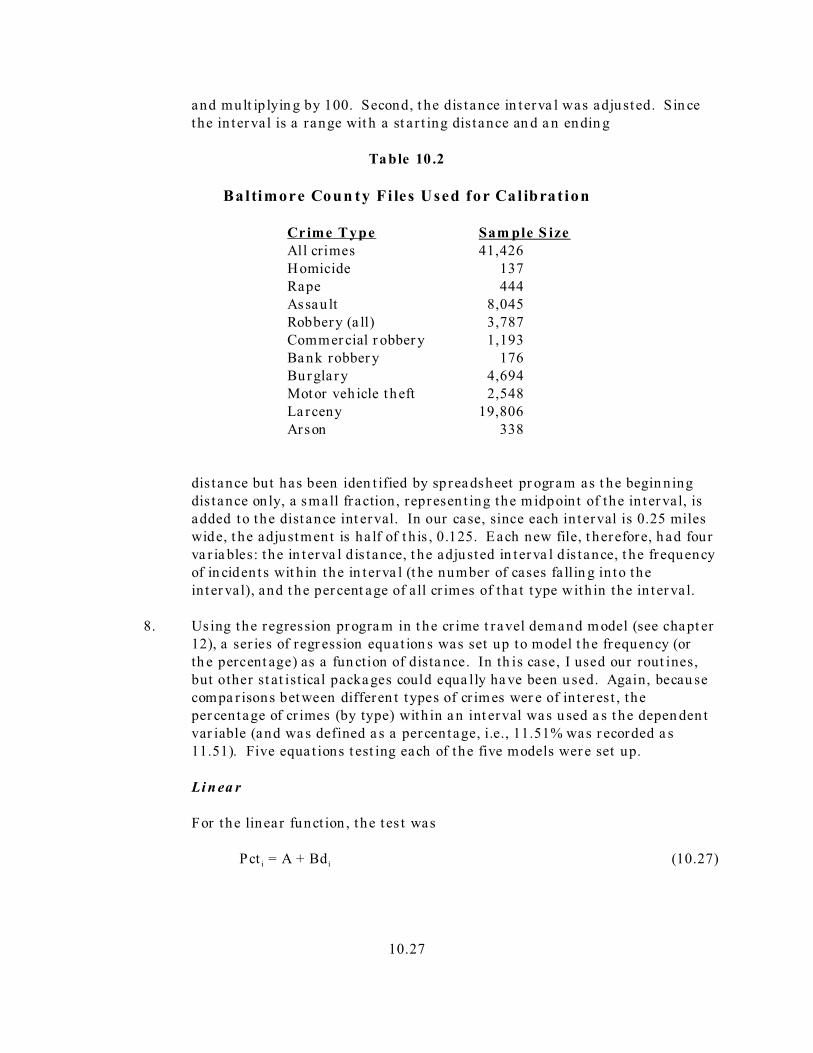
4. Th e r ecords wer e sort ed in to sub-groups based on differen t types of cr imes. For the Balt imore Coun ty example, eleven cat egor ies of cr ime incident wereused. Table 10.2 presen t s t he categories wit h their respective sa mple sizes. Of course, ot her sub-gr oups could have been iden t ified. E ach sub-gr oup wassa ved as a sepa ra te file. The same r ecords can be par t of mult iple files (e.g.,a record could be included in the ‘a ll robber ies’ file a s well a s in the‘commercial robber ies’ file). All r ecords wer e included in the ‘a ll cr imes ’ file.

5. For each type of cr ime, t he file was grouped in to dist ance int ervals of 0.25miles each. This involved t wo st eps. F irs t , th e dist ance between theoffender ’s r es idence and t he cr ime loca t ion was sort ed in ascen din g order . Second, a frequ ency distr ibut ion was condu cted on the dist ances a nd groupedint o 0.25 mile in tervals (oft en ca lled bins). The degree of pr ecision indis tance would depend on the size of the da ta set . F or 41,426 records,quar ter mile bins were appr opr iat e.

6. For each t ype of crim e, a new file was crea ted wh ich in cluded only t hefr equency d is t ribu t ion of t he d is t ances broken down in to qua r t er miledis tance inter va ls, d i.

7. In order to compa re differen t types of cr imes , which will have differen tfrequ en cy dist r ibu t ions , two new var iables wer e crea ted. Fir st , thefrequ en cy in the in ter val wa s conver ted in to th e per cent age of a ll cr imes of inea ch in ter va l by dividin g the frequ en cy by the t ota l number of inciden t s, N ,

10.27

and mult ip lyin g by 100. Second, t he dis t ance in terva l was adju sted. Sin cethe in ter val is a range wit h a st a r t ing dis t ance an d a n endin g

Ta ble 10 .2

Baltimore Coun ty Fi les Used for Cal ibrat ion

Crime Type Sam ple S izeAll crimes 41,426Homicide 137Rape 444Assau lt 8,045Robbery (a ll) 3,787Commer cial r obber y 1,193Ba nk robber y 176Burgla ry 4,694Motor veh icle t heft 2,548La rceny 19,806Arson 338

dis tance but has been iden t ified by sprea dsheet pr ogram as t he begin n ingdis tance on ly, a small fr action, represen t ing the m idpoin t of the in ter val, isadded to the dist ance int erval. In our case, since each in terval is 0.25 mileswide, t he adju stment is ha lf of t h is , 0.125. E ach new file, t herefore, h ad fourva r ia bles: the in terva l d is t ance, t he adju sted in terva l d is t ance, t he frequencyof in ciden t s wit h in the in terva l (t he number of cases fa llin g in to thein ter val), and t he per cent age of a ll cr imes of tha t type with in the in ter val.

8. Us ing the regression pr ogra m in t he cr ime t ravel dem and m odel (see chapt er12), a ser ies of regr ession equa t ion s was set up to model t he frequency (orth e percent age) as a fun ction of dista nce. In th is case, I used our rout ines,but other st at istical packa ges could equa lly ha ve been u sed. Again, becau secompa r isons bet ween differen t types of cr imes wer e of in ter es t , theper centage of cr imes (by type) with in a n int erval was u sed a s t he depen den tvar iable (and wa s defined a s a per centage, i.e., 11.51% was r ecorded a s11.51). Five equa t ions t est ing each of the five models wer e set up.

Li n ea r

For the linear funct ion , the t es t was

Pct i = A + Bd i (10.27)

10.28

where Pct i is t he per centage of a ll crim es of tha t type fallin g in to int er va l i, d i

is the dis t ance for in terva l i, A is the in tercept , a nd B is the slope. A a nd Bare es t imated dir ect ly from the r egr ession equ a t ion.

Nega t i ve Exponen t ia l

For the negat ive exponent ial funct ion , th e var iables h ave to be tr ansformedto est imate t he paramet er s. Th e fun ction is

-B*d i

Pct i = A * e (10.28)

A new va r ia ble is defin ed which is the na tura l loga r it hm of the percen tage ofa ll crim es of tha t type fallin g in to th e in ter va l, ln (Pct i). This t erm was t henregr essed a ga inst the dist ance inter va l, d i.

ln (Pct i) = K - B*d i (10.29)

However , s in ce the or igin a l equa t ion has been t ransformed in to a logfunct ion , B is the coefficien t and A can be ca lcu la ted dir ect ly from

ln (Pct i) = ln (A) - B*d i (10.30)

A = eK (10.31)

If the percen tage in any bin was 0 (i.e., Pct i = 0), th en a value of -16 wastaken since the na tura l logar ith m of 0 cannot be solved (it appr oximates -16as the percen tage approaches 0.0000001).

N or m a l

For the normal funct ion , a m ore complex tr ansformat ion must be used. Thenorm al function in the m odel is

1 -0.5*Zij2

Pct i = A * ----------------------- * e (10.32) Sd* SQRT(2B)

First , a st an dar dized Z var iable for t he dist ance, d i, is crea ted

(d i - Mean D)Zi = ------------------- (10.33)

Sd

where Mean D is th e mean dista nce and S d is the st andard devia t ion ofdist ance. These a re ca lcu lat ed from t he or igina l da ta file (before crea t ing thefile of frequen cy dis t r ibu t ions). Second, a norm al t r ansform at ion of Z isconst ruct ed with

10.29

1 -0.5*Zij2

Normal(Zi) = -------------------- * e (10.34) Sd* SQRT(2B)

F ina lly, th e norm alized va r iable is regressed a gainst the per cent age of a llcrim es of tha t type fallin g in to th e in ter va l, Pct i wit h no cons tan t

Pct i = A* Normal(Zi) (10.35)

A is est ima ted by th e regression coefficient .

L og n or m a l

For t he lognorm al fun ction , anoth er complex t ransformat ion m ust be done. The lognormal fu nct ion for the percen tage of a ll cr im es of a type for apa r t icula r dis t ance int er val is

1 -[ln (d2i) - MeanD ]2 / 2 *Sd

2

P ct i = A * -------------------------- * e (10.36) d2

ij * Sd* SQRT(2B)

The t ransformat ion can be crea ted in s t eps. F irs t , crea te L

L = ln (d i2) (10.37)

Second, crea te M

M = (l - Mean D)2 (10.38)

Third , crea te O

mO = --------- (10.39) (2*S d

2)

Four th , crea te P by r a isin g e to the O t h power .

P = eO(10.40)

Fift h , cr ea te the lognormal con version , Lnormal

1 Lnormal(d i) = A * ----------------------------- * P (10.41)

d2ij * Sd* SQRT(2B)

F ina lly, th e lognormal var iable is regressed a gainst the per cent age of a llcr im es of tha t type fa llin g in to the in terva l, Pct i wit h no cons tan t

10.30

Pct i = A* Lnormal(d i) (10.42)

A is est ima ted with the regression coefficient .

Trunca ted Nega t i ve Exponen t ia l

For t he t runcat ed nega t ive exponent ia l fun ction , two models wer e set up. The fir st applied to the dis t ance range from 0 to the dis t ance a t which thepercentage (or frequ en cy) is h ighest , Ma xd i. The second a pp lied t o alldis t ances gr ea ter than th is dis t ance

Linear : Pct i = A + Bd i for d ij $ 0, d ij# Ma xd ij (10.43)

Nega t ive -C*di

Exponen t ia l: Pct i = A*e for d ij> Maxd ij (10.44)

To use t h is funct ion , th e user specifies the dist ance a t which the pea klikelih ood occurs, d p (the peak d istance) and the va lue for tha t peaklikelihood, P (th e peak likelihood ). For the n ega t ive exponent ia l fun ction , theuser specifies t he exponent , C.

In order to splice the two equa t ions t ogeth er (the spline), th e Crim eS tatt runca ted nega t ive exponent ia l r out in e st a r t s the linear equa t ion a t theorigin and ends it a t t he highest value. Thus,

A = 0 (10.45)

B = P/dp (10.46)

where P is the peak likelihood an d dp is the pea k d istance.

The exponent , C, can be est ima ted by tr ansforming the depen den t var iable,Pct i, as in the n ega t ive exponent ia l above (equa t ion 10.28) an d r egr essin g thena tura l log of the percen tage (ln (Pct i) aga inst the dist ance inter va l, d i, onlyfor those in terva ls tha t are grea ter than the peak dis tance. I have found tha test imat ing the t r ansform ed equ a t ion wit h a coefficien t , A in

-C*d i

Pct i = A * e (10.47)

ln (Pct i) = Ln(A) - C*d i (10.48)

gives a bet t er fit to th e equ a t ion . However , the u ser need only inpu t theexponent , C, in the J t c rou t ine a s t he coefficien t , A, of the n ega t iveexponent ia l is ca lcu la ted in terna lly t o produce a dis t ance va lu e a t which thepeak likelihood occur s. Th e formula is:

10.31

ln(P) + C*(dp - d i)

A = e (10.49)

wh er e P is t he pea k likelih ood, d p is t he dist ance for t he pea k likelihood, C isan exponent (assu med to be positive) an d d i is the dis t ance in terva l for theh is togram.

9. Once the pa rameters for the five models h ave been est ima ted, th ey can becompared to see which one is best a t predict in g t he t r avel behavior for apa r t icu lar type of cr ime. It is to be expected t ha t differen t types of cr imeswill have d ifferen t op tima l models and tha t t he parameter s will a lso va ry.

Exam ples from B alt imore County

Let ’s illu st ra te wit h the Ba lt im ore Cou nty da ta . F igure 10.4 shows the frequencydist r ibut ion for a ll types of cr ime in Balt imore Coun ty. As can be seen , at the nearestdis t ance in terva l (0 to 0.25 miles wit h an assigned ‘adjusted’ midpoin t of 0.125 miles),about 6.9% of a ll cr imes occur with in a qua r ter mile of the offender ’s r esiden ce (it can beseen on the Y-axis). However, for the next in terval (0.25 to 0.50 miles with an assignedmidpoint of 0.375 m iles), alm ost 10% of a ll crim es occur a t tha t dis t ance (9.8%). Insu bsequ ent int ervals, however, t he per centage decreases, a lit t le less t han 6% for 0.50 to0.75 m iles (wit h the m idpoin t bein g 0.625 m iles), a lit t le more t han 4% for 0.75 to 1 mile(th e m idpoint is 0.875 miles), an d so fort h .

The bes t fit t ing st a t ist ical function wa s t he nega t ive exponen t ia l. The par t icula requ a t ion is

-0.229*d iPct i = 5.575 *e (10.50)

This is shown with the solid line. As can be seen , th e fit is good for most of the dist ances,though it underest imates a t close t o zer o dist ance an d overest imates from about a ha lf mileto about four miles. There is only sligh t evidence of decreased act ivit y n ear to the loca t ionof the offender .

However , the dist r ibu t ion va r ies by t ype of crim e. Wit h the Ba lt imore County da ta ,pr oper ty cr imes , in gener a l, occur fa r ther away th an per sona l cr imes . The t runca tednega t ive exponent ia l genera lly fit proper ty cr im es bet t er , lendin g suppor t for theBran t ingham and Bran t ingham (1981) framework for these types . For example, la rcenyoffender s h ave a definite sa fety zone around t heir r esidence (figure 10.5). Fewer than 2%of la rceny thefts occur wit h in a qu ar ter mile of the offender ’s r es idence. However , thepercentage jumps to about 4.5% from a qu ar ter mile t o a h a lf. The t runcat ed nega t iveexponen t ia l funct ion fit s t he dat a r easonably well t hough it overes t ima tes from abou t 1 to3 miles and u nderest imat es from a bout 4 to12 miles.

Journey to Crime Distances: All CrimesNegative Exponential Distribution

Perc

ent o

f all

crim

esFigure 10.4:

Number of trips for distance bin

Fitted function

Distance from offender's home (miles)

05

1015

2025

10%

8%

6%

4%

2%

0%

Negative exponential

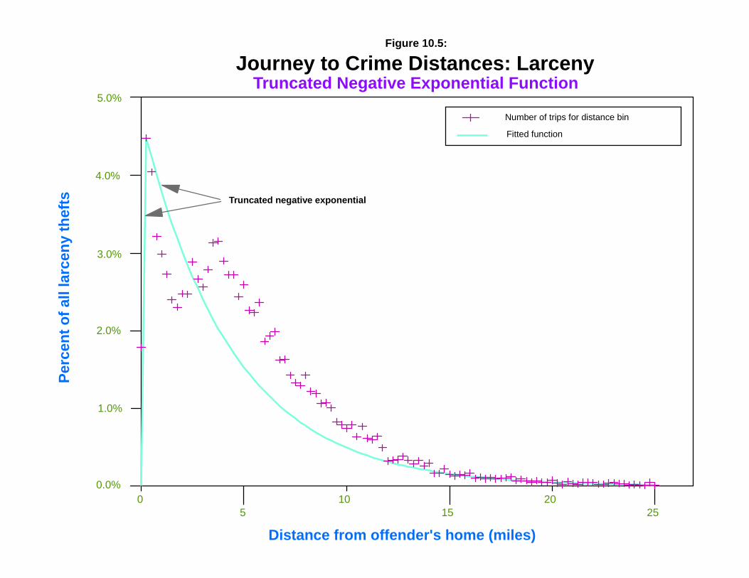
Journey to Crime Distances: LarcenyTruncated Negative Exponential Function

Figure 10.5:

05

1015

2025

5.0%

4.0%

3.0%

2.0%

1.0%

0.0%

Perc

ent o

f all

larc

eny

thef

ts

Distance from offender's home (miles)

Number of trips for distance bin

Fitted function

Truncated negative exponential

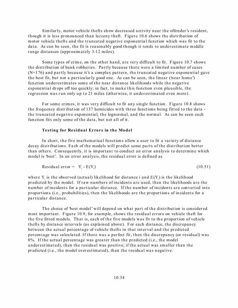
10.34

Similar ly, motor vehicle theft s sh ow decrea sed a ct ivity near the offender ’s r esiden t ,though it is less pronounced than la rceny t heft . F igure 10.6 shows the dis t r ibu t ion ofmotor veh icle theft s and the t runca ted nega t ive exponent ia l fu nct ion which was fit to theda ta . As can be seen , the fit is rea sonably good though it t en ds to un derest imate m iddlerange dis t ances (approxim ately 3-12 miles).

Some types of cr im e, on the other hand, a re very d ifficu lt to fit . F igure 10.7 showsthe dist r ibut ion of bank r obber ies. Pa r t ly because t here were a limited number of cases(N=176) and par t ly because it ’s a complex pa t t er n , the t runcat ed nega t ive exponent ia l gavethe best fit, bu t not a pa r t icu lar ly good one. As can be seen , th e linear (‘near home’)funct ion underes t ima tes some of t he nea r dis t ance likelihoods wh ile t he nega t iveexponent ia l dr ops off too quickly; in fact , to ma ke t h is function even pla usible, t heregr ession wa s r un only u p t o 21 miles (other wise, it underest imated even more).

For some cr im es, it was very d ifficu lt to fit any s in gle funct ion . F igure 10.8 showsthe frequency distr ibut ion of 137 homicides wit h th ree funct ions being fit t ed t o the da ta -the t runca ted nega t ive exponent ia l, the lognormal, and the normal. As can be seen eachfun ction fit s only some of the da ta , bu t not a ll of it .

Test ing for Res idual Errors in the Model

In shor t , t he five mathemat ica l fu nct ion s a llow a user to fit a va r iety of dis t ancedecay dist r ibut ions. Ea ch of the models will pr edict some pa r t s of the dist r ibut ion bet t erthan others. Consequent ly, it is im por tan t to conduct an er ror ana lysis to determin e whichmodel is ‘best’. In an error an alysis, th e residua l error is defined as

Residu a l er ror = Yi - E(Yi) (10.51)

where Yi is the observed (actua l) lik elihood for dis t ance i and E(Yi) is the likelihoodpr edicted by th e model. If raw numbers of inciden t s a re used, t hen the likelihoods a re thenumber of inciden t s for a pa r t icula r dis t ance. If the number of inciden t s a re conver ted in topropor t ion s (i.e., probabilit ies), t hen the likelihoods a re the propor t ion s of in ciden t s for apa r t icula r dis t ance.

The choice of ‘best model’ will depen d on what pa r t of the dist r ibut ion is consider edmost im por tan t . F igure 10.9, for exa mple, shows the residua l er rors on veh icle theft forthe five fit t ed models. Th a t is, ea ch of the five models was fit to th e propor t ion of veh icletheft s by dis t ance in terva ls (as expla in ed above). F or each dis t ance, t he discrepancybetween the actua l percentage of vehicle th eft s in tha t int erval and t he pr edictedpercen tage was calcu la ted. If there was a per fect fit , t hen the discrepancy (or residua l) was0%. If the actua l percentage was grea ter than the pr edicted (i.e., th e modelunder est ima ted), then the residu a l was positive; if the actua l was sm aller t han thepr edicted (i.e., t he m odel overest imated), th en the r es idu a l wa s n ega t ive.

Journey to Crime Distances: Vehicle TheftTruncated Negative Exponential Function

Figure 10.6:

05

1015

2025

6%

5%

4%

3%

2%

1%

0%

Perc

ent o

f all

vehi

cle

thef

ts

Number of trips for distance bin

Fitted function

Distance from offender's home (miles)

Truncated negative exponential

Journey to Crime Distances: Bank RobberyTruncated Negative Exponential Function

Perc

ent o

f all

bank

robb

erie

s

05

1015

2025

6%

4%

2%

0%

Figure 10.7:

Distance from offender's home (miles)

Number of trips for distance bin

Truncated negative exponential

Fitted function

Journey to Crime Distances: HomicideNormal, Lognormal, and Truncated Negative Exponential Functions

Normal

Lognormal

Truncated negative exponential

Figure 10.8:

05

1015

2025

14%

12%

10%

8%

6%

4%

2%

0%

Perc

ent o

f all

hom

icid

es

Distance from offender's home (miles)

Number of trips for distance binFitted normal function

Fitted truncated negative exponential functionFitted lognormal function

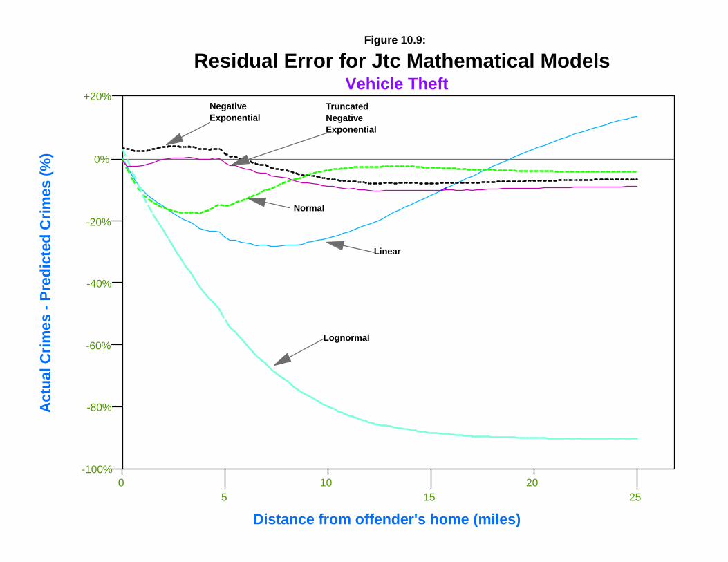
Vehicle Theft

Act

ual C

rimes

- Pr

edic

ted

Crim

es (%

)

Linear

Lognormal

Negative Exponential

TruncatedNegativeExponential

Residual Error for Jtc Mathematical Models

Normal

Figure 10.9:

05

1015

2025

+20%

0%

-20%

-40%

-60%

-80%

-100%

Distance from offender's home (miles)

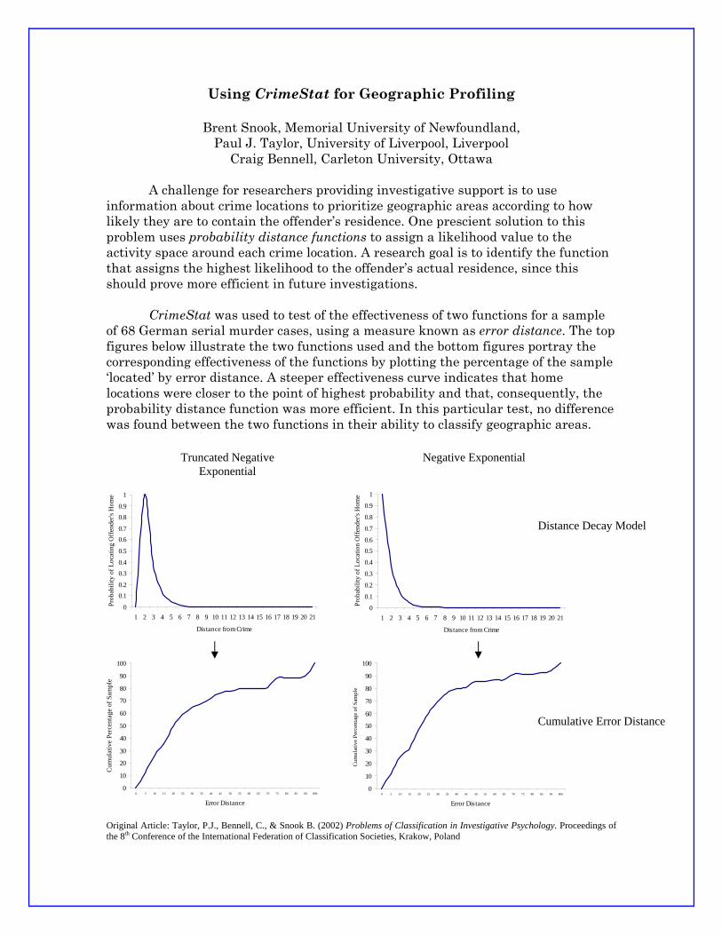
Using CrimeStat for Geographic Profiling

Brent Snook, Memorial University of Newfoundland, Paul J. Taylor, University of Liverpool, Liverpool

Craig Bennell, Carleton University, Ottawa

A challenge for researchers providing investigative support is to use information about crime locations to prioritize geographic areas according to how likely they are to contain the offender’s residence. One prescient solution to this problem uses probability distance functions to assign a likelihood value to the activity space around each crime location. A research goal is to identify the function that assigns the highest likelihood to the offender’s actual residence, since this should prove more efficient in future investigations. CrimeStat was used to test of the effectiveness of two functions for a sample of 68 German serial murder cases, using a measure known as error distance. The top figures below illustrate the two functions used and the bottom figures portray the corresponding effectiveness of the functions by plotting the percentage of the sample ‘located’ by error distance. A steeper effectiveness curve indicates that home locations were closer to the point of highest probability and that, consequently, the probability distance function was more efficient. In this particular test, no difference was found between the two functions in their ability to classify geographic areas. Original Article: Taylor, P.J., Bennell, C., & Snook B. (2002) Problems of Classification in Investigative Psychology. Proceedings of the 8th Conference of the International Federation of Classification Societies, Krakow, Poland

0

0.1

0.2

0.3

0.4

0.50.6

0.7

0.8

0.9

1

1 2 3 4 5 6 7 8 9 10 11 12 13 14 15 16 17 18 19 20 21

Distance from Crime

Prob

abili

ty o

f Loc

atio

n O

ffen

der's

Hom

e

0

0.10.2

0.30.4

0.5

0.60.7

0.80.9

1

1 2 3 4 5 6 7 8 9 10 11 12 13 14 15 16 17 18 19 20 21

Distance from Crime

Prob

abili

ty o

f Loc

atin

g O

ffen

der's

Hom

e

0

10

20

30

40

50

60

70

80

90

100

0 5 10 15 20 25 30 35 40 45 50 55 60 65 70 75 80 85 90 800

Error Distance

Cum

ulat

ive

Perc

enta

ge o

f Sam

ple

0

10

20

30

40

50

60

70

80

90

100

0 5 10 15 20 25 30 35 40 45 50 55 60 65 70 75 80 85 90 800

Error Distance

Cum

ulat

ive

Perc

enta

ge o

f Sam

ple

Negative Exponential

Truncated Negative Exponential

Distance Decay Model

Cumulative Error Distance

10.40

As can be seen in figure 10.9, the t runca ted nega t ive exponen t ia l fit the da ta wellfrom 0 to about 5 miles, but t hen becam e poorer t ha n oth er models for longer dista nces. The nega t ive exponent ia l m odel was not as good as the t runca ted for dis t ances up to about5 miles, bu t was bet t er for dis t ances beyon d tha t poin t . The normal d is t r ibu t ion was goodfor dista nces from a bout 10 miles and far th er. The lognorm al was not pa rt icular ly good forany dista nces oth er than a t 0 miles, nor was t he linear .

The degree of pr edicta bility var ied by type of cr ime. For some types , pa r t icula r lypr oper ty cr imes , th e fit wa s r easona bly good. I obta ined R2 in the order of 0.86 to 0.96 forbu rglary, robbery, assau lt , larceny, a nd a u to th eft . For other types of crim e, pa r t icula r lyviolen t crim es, the fit was n ot ver y good with R2 values in the order of 0.53 (rape), 0.41(a r son) and 0.30 (homicide). These R2 va lu es were for the en t ir e dis t ance range; for anypa r t icula r dis t ance, however , the predicta bilit y var ied from ver y high to very low.

In modeling dis t ance decay with a mathem at ical function, a user has t o decidewhich par t of the dis t r ibu t ion is the most im por tan t as no sim ple mathemat ica l fu nct ionwill normally fit a ll the da ta (even approximately). In these cases , I a s sumed tha t the neardist ances wer e more impor tan t (up t o, say, 5 miles) and, th erefore, selected t he modelwhich ‘best ’ fit those dis t ances (see table 10.2). H owever , it was not a lways clea r whichmodel was best , even wit h tha t limited crit er ia .

P r ob le m s w i th Ma th e m a ti ca l D is ta n ce D e ca y F u n ct io n s

There a re severa l r easons tha t mathemat ica l m odels of dis t ance decay dis t r ibu t ion s,su ch as illust ra ted in t he J t c rou t ine, do not fit da ta very well. Fir st , as m ent ioned ea r lier,few cit ies have a completely sym met r ical gr id s t ructu re or even one t ha t is a pproximatelygr id-like (th er e a re except ions, of course). Limita t ions of ph ysical topograph y (moun ta ins,oceans, r ivers, lakes) as well as differen t h istor ica l developm ent pa t t erns m akes t r avelasym met r ical a roun d m ost loca t ions .

Second, t here is popula t ion densit y. Sin ce most met ropolit an a reas have muchhigher int ensity of lan d u se in the cen ter (i.e., more act ivities a nd facilities), t r avel t ends t obe dir ected towards h igher la nd use in tensit y t han away fr om them. F or or igin loca t ion stha t ar e not dir ect ly in t he cent er, t r avel is more likely to go towards t he cent er t han awa yfrom it .

This would be tr ue of an offender as well. If the per son wer e lookin g for eith erper sons or proper ty as ‘t a rgets’, th en t he offender would be more likely to t r avel towardsthe met ropolita n cen ter than away from it. Since most met ropolita n cen ters h ave st reetnet works t ha t wer e la id ou t much ear lier , the s t reet net work ten ds to be ir regu la r . Consequent ly, t r ips will va ry by loca t ion wit h in a met ropolit an a rea . One would expectsh or ter t r ips by an offender living close t o the met ropolita n cen ter than one living fa r theraway; sh or ter t r ips for offender s living in m ore built -up a reas t han in lower den sity ar eas;sh ort er t r ips for offender s in mixed u se neighborh oods than in st r ictly r esiden t ia lneighborh oods ; an d so fort h . Thus, t he dist r ibu t ion of t r ips of any sort (in our case, crim et r ips from a residen t ia l locat ion to a cr ime loca t ion), will t en d t o follow a n ir regu lar ,

10.41

dist ance decay type of dist r ibut ion . Simple m athemat ica l models will not fit the da ta verywell an d will ma ke ma ny errors.

Thir d, t he select ion of a best mathemat ica l fu nct ion is pa r t ly dependent on theint erva l size used for the bins. In t he above examples, an int erva l size of 0.25 miles wasused to calcu la te the frequency dis t r ibu t ion . With a differen t in terva l s ize (e.g., 0.5 miles),however , a sligh t ly differen t dis t r ibu t ion is obt a in ed. This effect s the mathemat ica lfunct ion tha t is selected as well a s the pa rameters tha t are es t imated . For example, theissue of whet her ther e is a sa fety zone nea r the offender ’s r esidence from which t her e isdecreased a ctivit y or not is pa r t ly depen dent on t he in ter val size. With a sm all inter val,the zone may be det ected wh er ea s with a sligh t ly larger in ter val the subt le dis t inction inmeasu red distan ces may be lost. On th e oth er ha nd, having a sma ller interval may lead tounreliable est ima tes sin ce there may be few cases in the int erval. Ha ving a t echniquedepend on the in terva l s ize makes it vu ln erable to mis -specifica t ion .

U s e s o f Ma th e m a ti ca l D is ta n ce D e ca y F u n ct io n s

Does t h is m ea n tha t one should not u se mathem at ical dist ance functions? I wouldargu e tha t under most cir cumstances, a mathemat ica l fu nct ion will give less precis ion thanan empir ica lly-der ived one (see below). However , th ere are two cases wh en amathemat ica l model would be appr opr iat e. First , if there is eith er no da ta or insufficientda ta to model t he em pir ical t r avel dist r ibu t ion, t he u se of a mathem at ical m odel can serveas a n appr oximat ion . If the user has a good sen se of wha t the dist r ibut ion looks like, t hena mathem at ical m odel may be u sed t o appr oximate t he dist r ibu t ion . However , if a poor lydefin ed funct ion is selected, t hen the selected funct ion may produce many er rors.

A second case when mathemat ica l models of d is tance decay would be appropr ia te isin t heory developm ent or applica t ion . Man y models of t r avel beha vior , for exam ple,assume a sim ple dis t ance decay type of function in order sim plify the a llocat ion of t r ipsover a region . This is a common procedure in t r avel demand modeling where t r ips fromeach of many zones a re assigned to every ot her zon e usin g a gr avity t ype of funct ion(St oph er and Meybur g, 1975; Field an d Ma cGregor , 1987). Even t hough t he modelproduces er rors because it assumes un ifor m t ravel behavior in a ll dir ect ion s, t he er rors a recor rected la ter in the m odeling pr ocess by adjust ing the coefficien t s for a llocat ing t r ips topar t icu la r roads (t r a ffic a ssignment ). The model provides a sim ple device and the er rorsa re corrected down the line. St ill, I would argu e tha t an empir ica lly-der ived dis t r ibu t ionwill p roduce fewer er ror s in a lloca t ion and, t hus, r equ ir e les s adjustmen t la t er on . E r ror scan never help a model and it s bet t er to get it more corr ect in it ia lly to ha ve to adjus t itla t er on; the adjust men t may be inadequ a te. Never theless, t h is is common practice int ransport a t ion p lanning.

The J ou rn e y t o Crim e Ro u tin e Us in g a Math e m at ic al F orm u la

The J tc rou t ine wh ich a llows m athemat ica l modeling is sim ple to use. Figur e 10.10illu st ra tes how the user specifies a mathemat ica l fu nct ion . The rout in e requir es the use ofa gr id which is defined on the r efer en ce file t ab of the progra m (see cha pt er 3). Then , the

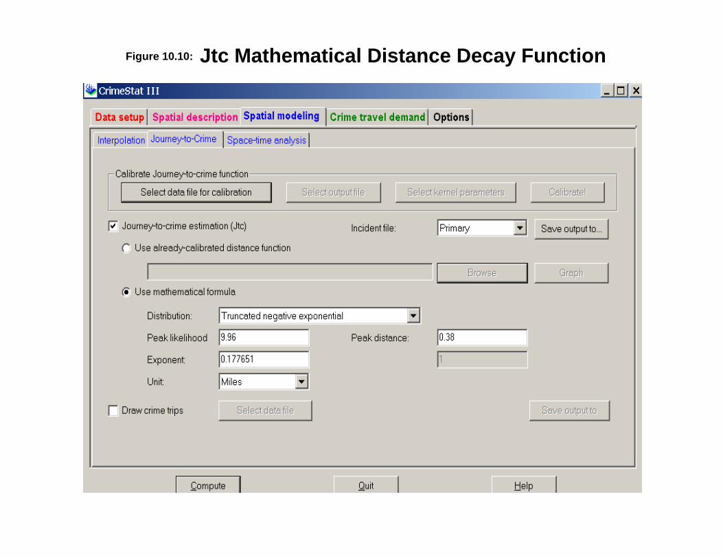
Jtc Mathematical Distance Decay FunctionFigure 10.10:

10.43

user must specify the m athem at ical function and t he paramet er s. In the figure, t het runca ted n egat ive exponent ial is being defined. The u ser must input values for the pea klikelih ood, t he pea k dis t ance, and t he exponent (see equ a t ions 10.43 a nd 10.44 above). Inthe figure, s in ce the ser ia l offenses were a ser ies of 18 robber ies, t he parameter s forrobbery ha ve been en tered int o the pr ogra m screen . The pea k likelihood wa s 9.96%(entered a s a whole nu mber - i.e., 9.96); the dist ance a t which th is pea k likelihood occur redwas the second dis t ance in terva l 0.25-0.50 miles (with a mid-poin t of 0.38 miles); and theest imated exponent wa s 0.177651. As m en t ioned a bove, the coefficien t for the n ega t iveexponent ia l pa r t of the equa t ion is est imated in ter na lly.

Table 10.3 gives the pa rameters for the ‘best ’ models wh ich fit t he da ta for the 11types of cr im e in Ba lt im ore Cou nty. For severa l of t hese (e.g., bank robber ies), t wo or morefunct ions gave approxima tely equa lly good fit s . Note tha t t hese parameter s wereest im ated wit h the Ba lt im ore Cou nty da ta . They will n ot fit any ot her ju r isdict ion . If auser wishes to apply th is logic, then the parameter s should be est im ated anew fromexist in g da ta . Never theless, on ce they h ave been ca libra ted, t hey ca n be used forpredictions.

The rou t ine can be ou tpu t t o ArcView , MapIn fo, Atlas*GIS , S urfer for Windows,S pat ial Analyst , and a s a n Ascii grid file wh ich can be r ea d by many oth er GIS packa ges. All bu t S urfer for Windows r equ ire t ha t the r efer en ce grid be crea ted by Crim eS tat.

Distance Model ing Using an Empir ica l ly Determined Fu nct ion

An a lter na t ive to mathemat ica l modeling of dist ance decay is to empirically describethe journey to cr ime d ist r ibut ion and t hen use t h is empir ica l funct ion to est ima te theresidence locat ion. Crim eS tat has a two-dim ension a l k ernel densit y r out in e tha t canca libra te the d is tance funct ion if p rovided da ta on t r ip or igins and des t ina t ions . The logicof ker nel dens ity est ima t ion was descr ibed in cha pt er 8, an d won’t be repea ted h ere.Essen t ia lly, a sym met r ical function (th e ‘ker nel’) is pla ced over ea ch point in a dis t r ibu t ion. The dis t r ibu t ion is then referenced rela t ive to a sca le (an equa lly-spaced line for two-dim ension a l k ernels and a gr id for th ree-dim ension a l k ernels ) and the va lu es for eachker nel a re summed a t each r eferen ce locat ion . See cha pt er 8 for deta ils.

Calibrate Kerne l Dens i ty Funct ion

The Crim eS tat ca libra t ion rou t ine a llows a user t o descr ibe the d is t ance d is t ribu t ionfor a sample of jou rney to cr ime t r ip s. The r equ ir emen t s a re tha t :

1. Th e da ta set must have the coordin a tes of both an origin locat ion a nd ades t ina t ion loca t ion ; and

2. The r ecords of a ll or igin and dest ina t ion locat ions h ave been popu la ted wit hlegit im ate coordin a te va lu es (i.e ., no unmatched records a re a llowed).

10.44

Ta ble 10 .3

J ou rney to Crime Mathe matic al Mode ls for Balt imore Coun tyParameter Est imates for Percentage Dis tr ibut ion

(Sam ple Sizes in P ar enth eses)

ALL CRIMES

Nega t ive Exponen t ia l: Coefficien t : 5.575107Exponen t : 0.229466

HOMICID E

Trunca tedNega t ive Exponen t ia l: Peak likelihood 14.02%

Peak dis tance 0.38 milesExponen t 0.064481

RAP E

Lognormal: Mean 3.144959St anda rd Devia t ion 4.546872Coefficient 0.062791

ASSAULT

Trunca tedNega t ive Exponen t ia l: Peak likelihood 27.40%

Peak dis tance 0.38 milesExponen t 0.181738

ROBBERY

Trunca tedNega t ive Exponen t ia l: Peak likelihood 9.96%

Peak dis tance 0.38 milesExponen t 0.177651

COMMERCIAL ROBBERY

Trunca tedNega t ive Exponen t ia l: Peak likelihood 4.9455%

Peak dis tance 0.625 milesExponen t 0.151319

10.45

Ta ble 10 .3 (con t inu ed)

BANK ROBBERY

Trunca tedNega t ive Exponen t ia l: Peak likelihood 9.96%

Peak dis tance 5.75 milesExponen t 0.139536

BURGLARY

Trunca tedNega t ive Exponen t ia l: Peak likelihood 20.55%

Peak dis tance 0.38 milesExponen t 0.162907

AUTO THEFT

Trunca tedNega t ive Exponen t ia l: Peak likelihood 4.81%

Peak dis tance 0.63 milesExponen t 0.212508

LARCENY

Trunca tedNega t ive Exponen t ia l: Peak likelihood 4.76%

Peak dis tance 0.38 milesExponen t 0.193015

ARSON

Trunca tedNega t ive Exponen t ia l: Peak likelihood 38.99%

Peak dis tance 0.38 milesExponen t 0.093469

10.46

Da ta S et D efin it ion

The steps a re r ela t ively easy. F ir st , the u ser defines a calibr a t ion da ta set wit hboth origin and dest ina t ion locat ions. F igure 10.11 illust ra tes th is process. As wit h theprima ry and seconda ry files, th e rout ine reads ArcView ‘sh p’, dBase ‘dbf’, Ascii ‘txt ’, andMapIn fo ‘da t ’ files. For both the or igin loca t ion (e.g., the home residen ce of the offender )and t he dest ina t ion loca t ion (i.e., the cr ime loca t ion), th e names of the var iables for the Xand Y coordin a tes must be iden t ified as well a s t he t ype of coordin a te syst em and da ta un it(see chapter 3). In the example, t he or igin loca t ion s has va r iable names of H om eX andHomeY and the dest in a t ion loca t ion s has va r ia ble names of Inciden tX and Inciden tY forthe X and Y coordin a tes of the t wo locat ions r espectively. However , any name is a cceptableas long as th e two locat ions a re distinguished.

The u ser sh ould specify whet her ther e a re any miss ing values for these four fields(X and Y coordin a tes for both origin and dest ina t ion locat ions ). By defau lt , Crim eS tat willignore r ecords wit h blank values in any of th e eligible fields or r ecords wit h non-numer icvalues (e.g.,alph anumer ic character s, #, *). Blanks will a lways be excluded u n less t he userselect s <n one>. Th ere a re 8 possible opt ion s:

1. <bla nk> fields a re au toma t ically excluded. This is the defau lt2. <none> indicates tha t no records will be excluded. If th er e is a blank field,

Crim eS tat will tr eat it a s a 03. 0 is excluded4. –1 is excluded5. 0 and –1 ind ica tes t ha t both 0 an d -1 will be excluded6. 0, -1 and 9999 indica tes t ha t a ll th ree values (0, -1, 9999) will be excluded

Any other numer ical va lue can be t r ea ted as a miss ing value by t ypin g it (e.g.,99)Mult iple n umer ical va lues can be t r ea ted as m iss ing values by typin g them , separa t ingeach by commas (e.g., 0, -1, 99, 9999, -99).

The progr am will ca lcu la te the dis t ance between the or igin loca t ion and thedest ina t ion loca t ion for each record. If the un its a re sph er ica l (i.e., lat /lon), th en theca lcu lat ions u se spher ica l geomet ry; if the un its a re pr ojected (either meters or feet ), th enthe calcu la t ion s a re Euclidean (see chapter 3 for deta ils).

K er n el P a r a m et er s

Next , the u ser must define the ker nel paramet er s for calibra t ion. Th er e a re fivechoices tha t have to be made (Figure 10.12):

1. The method of int erpola t ion . As with the two-dimensiona l ker nel techn iquedescr ibed in chapter 8, t here a re five possible kernel fu nct ion s:

Jtc Calibration Data InputFigure 10.11:

Jtc Calibration Kernel ParametersFigure 10.12:

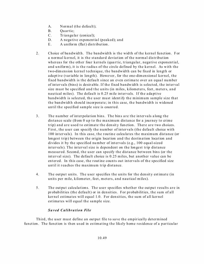
10.49

A. Normal (the defau lt );B. Qu ar t ic;C. Tr ia ngu la r (conica l);D. A nega t ive exponent ia l (peaked); andE. A unifor m (fla t ) dis t r ibu t ion .

2. Choice of ba ndwid th . The bandwid th is the wid th of the kernel fu nct ion . F ora normal k ernel, it is the st andard devia t ion of the normal d is t r ibu t ionwh er ea s for the oth er four ker nels (qua r t ic, t r iangular , nega t ive exponen t ia l,and u n iform), it is t he r adiu s of the circle defined by the ker nel. As with thetwo-dim ension kernel t echnique, t he bandwid th can be fixed in lengt h orada pt ive (var iable in len gth). However , for the one-dim en siona l ker nel, t hefixed bandwidt h is the defau lt s ince an even est ima te over a n equa l nu mberof in ter va ls (bin s) is desir able. I f th e fixed bandwidt h is select ed, the in ter va lsize must be specified and t he un it s (in miles , kilomet er s, feet , met er s, a ndnaut ical m iles). The defau lt is 0.25 m ile in ter va ls. I f th e a da pt ivebandwidt h is selected, th e user must ident ify th e minim um sa mple size th a tthe ban dwidt h sh ould incorpora te; in t h is case, th e ban dwidt h is widenedun til th e specified sam ple size is coun ted.

3. Th e n umber of in ter pola t ion bins. The bin s a re t he in ter va ls a long t hedis tance scale (from 0 u p t o th e m aximum dis tance for a journey to cr imet r ip) and a re u sed t o est imate t he den sit y fun ction . Ther e a re t wo choices . F ir st , the u ser can specify the number of in ter vals (the defau lt choice wit h100 in terva ls ). In th is case, t he rout in e ca lcu la tes the maximum dis tance (orlon gest t r ip ) between the or igin loca t ion and the dest in a t ion loca t ion anddivides it by th e specified nu mber of int ervals (e.g., 100 equa l-sizedin terva ls ). The in terva l s ize is dependent on the lon gest t r ip dis t ancemeasured. Second, t he user can specify the dis t ance between bin s (or theint erval size). The defau lt choice is 0.25 miles, but another value can been ter ed. In th is case , the r out ine counts ou t in ter va ls of th e specified sizeunt il it r eaches t he maximum t r ip dist ance.

4. The out pu t un it s. Th e u ser specifies the un it s for the den sit y est imate (inunit s per mile, k ilometer , feet , m eter s, a nd nau t ica l m iles).

5. The out pu t calcula t ions. Th e u ser specifies wh et her the out pu t resu lt s a re inpr obabilit ies (th e defau lt ) or in densit ies. For probabilit ies, the sum of a llker nel est ima tes will equa l 1.0. For den sit ies, th e su m of a ll ker nelest ima tes will equa l th e sa mple size.

Sa ved Ca l ibra t ion Fi l e

Third , th e user must define an ou tpu t file to sa ve th e empir ica lly det erminedfunct ion . The funct ion is then used in es t imat ing the likely home res idence of a par t icu la r

10.50

funct ion . The choices a re to save the file as a ‘dbf’ or Ascii t ext file. The saved file then canbe used in the J t c rout in e. F igure 10.13 illu st ra tes the outpu t file format .

C a l i br a t e

Four th , th e calibrat e but ton r un s th e rout ine. A calibrat ion window appear s an dindica tes the progress of the calcula t ions . When it is fin ish ed, the u ser can view a graphillust ra t ing the es t imated dis t ance decay function (Figu re 10.14). The purpose is t o providequ ick dia gnost ics to th e u ser on t he fun ction and select ion of the ker nel pa ramet er s. Wh ileth e gra ph can be print ed, it is not a high qua lity print. If a h igh qua lity gra ph is needed,the outpu t calibra t ion file should be im por ted in to a gr aph ics progra m.

Examples from Balt imore County

Let ’s illu st r a t e t h is method by showing the r esult s for t he same data set s t ha t wereca lcu la ted above in the mathemat ica l sect ion (figures 10.4-10.8). In a ll cases, t he normalker nel function wa s u sed. The ba ndwidt h wa s 0.25 m iles except for the ba nk robber y da taset , which had only 176 cases, and t he homicide da ta set , which on ly had 137 cases;because of the small sample sizes, a bandwid th of 0.50 miles was used for these two da taset s. The in terva l wid th selected was a dis t ance of 0.25 miles between bin s (0.5 miles forbank robberies an d homicides) an d probabilities were out put .

F igure 10.15 shows the kernel est im ate for a ll cr im es (41,426 t r ips). A fr equencydis t r ibu t ion was ca lcula ted for the same n umber of in ter va ls a nd is overla id on the gr aph .It was selected to be comparable to the mathemat ica l fu nct ion (see figure 10.4). Note howclosely the kernel es t imate fit s the da ta compared to the nega t ive exponen t ia lma th emat ical fun ction. The fit is good for every value but t he peak value; th at is becau sethe ker nel averages severa l in tervals t ogeth er to pr odu ce an est ima te.

F igure 10.16 sh ows t he ker nel est ima te for lar ceny th eft s. Again , th e ker nelmet hod pr oduces a much closer fit a s a compa r ison wit h figur e 10.5 will show. Figure10.17 shows t he ker nel es t imate for veh icle t hefts. F igure 10.18 sh ows the ker nel es t imatefor bank robber ies and figure 10.19 shows the kernel est im ate for homicides. An in spect ionof these gr aphs shows how well the kernel fu nct ion fit s the da ta , com pared to themathemat ica l funct ion , even when the da ta a re irr egula r ly spa ced (in vehicle th eft s, ban krobber ies, a nd homicides). F igure 10.20 compares the dis t ance decay fu nct ion s forhomicides committ ed agains t st r angers compa red to homicides committ ed agains t kn ownvictims.

In shor t , t he J t c ca libra t ion rout in e a llows a much closer fit to the da ta than any ofthe simpler mathemat ica l funct ions. While it ’s possible to produce a complexmathemat ica l fu nct ion tha t will fit the da ta more closely (e.g., h igher order polyn omia ls ),the ker nel met hod is m uch simpler to use a nd gives a good a ppr oximat ion to the da ta .

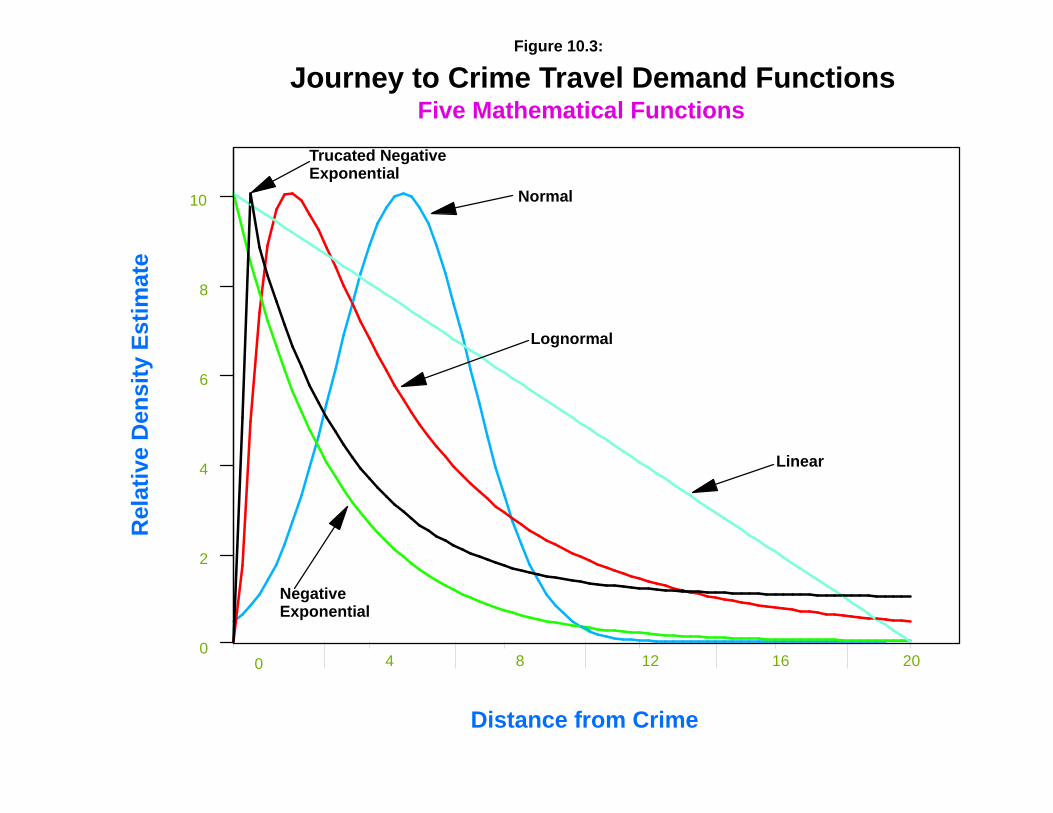
Journey to Crime Travel Demand FunctionsFive Mathematical Functions

Distance from Crime

Rel

ativ

e D

ensi

ty E

stim

ate

0 4 8 12 16 20

10

8

6

4

2

0

Trucated Negative Exponential

Negative Exponential

Normal

Lognormal

Linear

Figure 10.3:

Jtc Calibration Graphic OutputFigure 10.14:

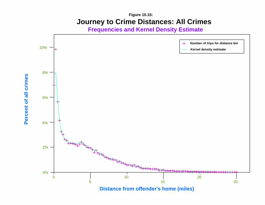
Journey to Crime Distances: All CrimesPe

rcen

t of a

ll cr

imes

05

1015

2025

10%

8%

6%

4%

2%

0%

Number of trips for distance bin

Kernel density estimate

Distance from offender's home (miles)

Frequencies and Kernel Density Estimate

Figure 10.15:

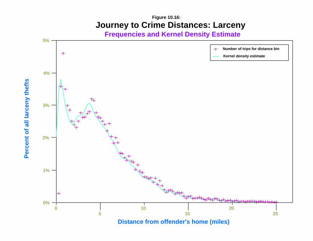
Journey to Crime Distances: LarcenyFigure 10.16:

Perc

ent o

f all

larc

eny

thef

ts

05

1015

2025

5%

4%

3%

2%

1%

0%

Number of trips for distance bin

Kernel density estimate

Distance from offender's home (miles)

Frequencies and Kernel Density Estimate

Journey to Crime Distances: Vehicle TheftPe

rcen

t of a

ll ve

hicl

e th

efts

05

1015

2025

5%

4%

3%

2%

1%

0%

Number of trips for distance bin

Kernel density estimate

Distance from offender's home (miles)

Frequencies and Kernel Density Estimate

Figure 10.17:

Journey to Crime Distances: Bank Robbery

Distance from offender's home (miles)

Perc

ent o

f all

bank

robb

erie

s

05

1015

2025

10%

8%

6%

4%

2%

0%

Number of trips for distance bin

Kernel density estimate

Frequencies and Kernel Density Estimate

Figure 10.18:

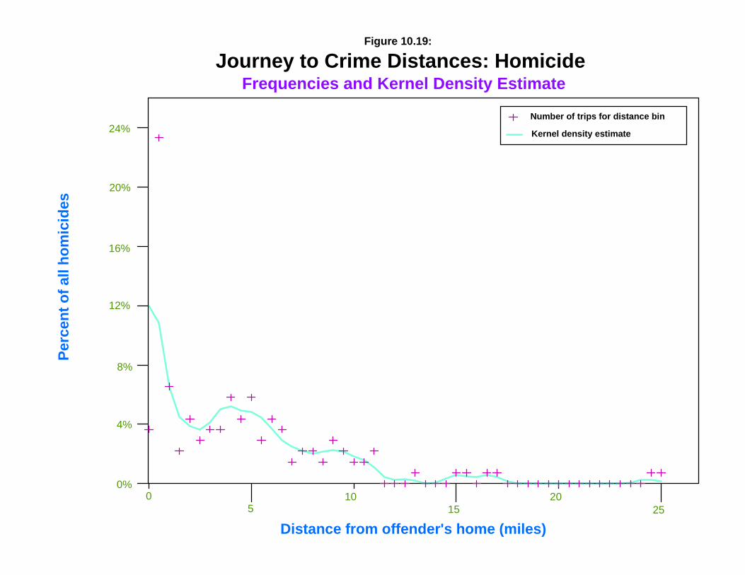
Journey to Crime Distances: HomicidePe

rcen

t of a

ll ho

mic

ides

05

1015

2025

24%

20%

16%

12%

8%

4%

0%

Number of trips for distance bin

Kernel density estimate

Distance from offender's home (miles)

Frequencies and Kernel Density Estimate

Figure 10.19:

Journey to Crime Distances: Homicide by Victim RelationshipFigure 10.20:

Perc

ent o

f all

hom

icid

es

(b

y vi

ctim

rela

tions

hip)

05

1015

2025

24%

20%

16%

12%

8%

4%

0%

Victim known

Stranger

Number of trips for distance bin

Kernel density estimate

Distance from offender's home (miles)

Frequencies and Kernel Density Estimate

Using Journey-To-Crime Routine for Journey-After-Crime Analysis

Yongmei Lu Department of Geography

Southwest Texas State University San Marcos, TX

The study of vehicle theft recovery locations can fill a gap in the knowledge about criminal travel patterns. Although the journey-to-crime routine of CrimeStat was designed to analyze the distance between offense location and offender’s residential location, it can be used to describe the distance between vehicle theft location and the corresponding recovery location. There were more than 3000 vehicle thefts in the City of Buffalo in 1998. Matching the offenses with vehicle recoveries in the same year, 1600 location pairs were identified for a journey-after-vehicle-theft analysis. To evaluate the randomness of the distances, 1000 groups of simulations were conducted. Every group contains 1600 simulated trips of journey-after-vehicle-theft. The results indicate that 1) short distances dominate journey-after-vehicle-theft, and 2) the observed trips are significantly shorter than the random trips given the distribution of possible vehicle theft and recovery locations.

0.000.010.020.030.040.050.060.070.080.09

0.00

1.59

3.17

4.76

6.34

7.93

9.51

11.10

12.68

14.27

15.85

17.44

19.02

20.61

22.19

distance from vehicle theft location (miles)

prob

abili

ty o

f rec

over

y

0.00

0.01

0.01

0.02

0.02

0.03

0.03

3.08

3.10

3.12

3.14

3.17

3.19

3.21

3.23

3.25

3.28

3.30

3.32

3.34

3.37

3.39

3.41

3.43

distance from theft location (miles)

prob

abili

ty o

f mea

ns

0.00

0.20

0.40

0.60

0.80

1.00

1.20

cum

ulat

ive

prob

abili

ty

Probability of recovering a stolen vehicle by distance from vehicle theft location

Distribution of mean distances of simulated vehicle theft-recovery location pairs.

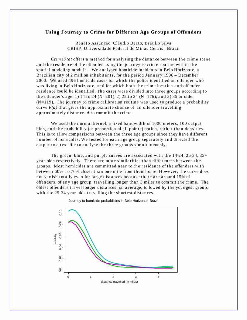
Using Journey to Crime for Different Age Groups of Offenders

Renato Assunção, Cláudio Beato, Bráulio Silva CRISP, Universidade Federal de Minas Gerais , Brazil

CrimeStat offers a method for analysing the distance between the crime scene

and the residence of the offender using the journey to crime routine within the spatial modeling module. We analysed homicide incidents in Belo Horizonte, a Brazilian city of 2 million inhabitants, for the period January 1996 – December 2000. We used 496 homicide cases for which the police identified an offender who was living in Belo Horizonte, and for which both the crime location and offender residence could be identified. The cases were divided into three groups according to the offender‘s age: 1) 14 to 24 (N=201); 2) 25 to 34 (N=176); and 3) 35 or older (N=119). The journey to crime calibration routine was used to produce a probability curve P(d) that gives the approximate chance of an offender travelling approximately distance d to commit the crime.

We used the normal kernel, a fixed bandwidth of 1000 meters, 100 output

bins, and the probability (or proportion of all points) option, rather than densities. This is to allow comparisons between the three age groups since they have different number of homicides. We tested for each age group separately and directed the output to a text file to analyse the three groups simultaneously.

The green, blue, and purple curves are associated with the 14-24, 25-34, 35+

year olds respectively. There are more similarities than differences between the groups. Most homicides are committed near to the residence of the offenders with between 60% t o 70% closer than one mile from their home. However, the curve does not vanish totally even for large distances because there are around 15% of offenders, of any age group, travelling longer than 3 miles to commit the crime. The oldest offenders travel longer distances, on average, followed by the youngest group, with the 25-34 year olds travelling the shortest distances.

distance travelled (in miles)

0 1 2 3 4

0.0

0.02

0.04

0.06

0.08

0.10

Journey to homicide probabilities in Belo Horizonte, Brazil

prob

abili

ty

10.61

The J ou rn e y t o Crim e Ro u tin e Us in g t h e Calib rat e d F ile

After the dis t ance decay fu nct ion has been ca libra ted and saved as a file, t he file canbe used t o ca lcu lat e the likelihood su r face for a ser ial offender . The u ser specifies the nameof the a lready-ca libra ted dis tance funct ion (as a ‘dbf’ or an Ascii t ext file) and the ou tpu tforma t . As with the ma themat ica l rou t ine, t he ou tpu t can be to ArcView , MapIn fo,Atlas*GIS , S urfer for Windows, S pat ial Analyst , an d a s a n Ascii gr id file which can be rea dby ma ny other GIS pa cka ges. All bu t S urfer for Windows r equire t ha t the reference grid becrea ted by Crim eS tat.

The result is produced in t hr ee steps:

1. The r out ine calcula tes the dist ance between each r eferen ce cell of the gr idand each in ciden t loca t ion ;

2. For each dis t ance measured, t he rout in e look s up the ca lcu la ted va lu e fromth e saved calibrat ion file; an d

3. For each reference gr id cell, it sums the va lu es of a ll the in ciden t s to producea single likelihood est ima te.

Ap pli ca ti on o f th e Ro u ti ne

To illus t ra te the techniques , th e resu lts of the two methods on a single case a recompa red. The case h as been selected because t he rou t ines accura tely est ima te theoffender ’s r es idence. This was done to dem ons t ra te h ow the t echniqu es work. In the n extsection, I’ll ask the qu est ion about how accura te t hese m et hods a re in gener a l.

Th e case in volved a man who had commit ted 24 offen ses. These in clu ded 13 theft s,5 bu rgla r ies, 5 assau lt s, a nd one rape. The spa t ia l d is t r ibu t ion was va r ied; many of theoffenses wer e clus tered bu t some wer e scat t ered. Since th ere were multiple t ypes of cr imescommitt ed by th is individua l, a decision had t o be made over which model to use t oest ima te the individua l’s r esiden ce. In t h is case, th e theft (lar ceny) model was selectedsin ce tha t wa s t he domin ant type of crim e for th is in dividua l.

For the mathemat ica l fu nct ion , t he t runca ted nega t ive exponent ia l was chosen fromtable 10.3 with the paramet er s bein g:

Peak likelihood 4.76%Peak dis tance 0.38 milesExponen t 0.193015

For t he ker nel den sit y model, t he calibr a ted fun ction for la rceny wa s select ed (figure10.16).

10.62

Figure 10.21 sh ows t he r esu lt s of the es t imat ion for the t wo met hods. Th e out pu t isfrom S urfer for Windows (Golden Software, 1994). The left pane shows the resu lt s of themathem at ical function wh ile the r ight pa ne shows t he r esu lt s for the ker nel densit yfunct ion . The in ciden t loca t ion s a re shown as cir cles while the actua l r esidence loca t ion ofthe offender is shown as a square. Sin ce th is is a sur face model, the h ighest loca t ion hasth e highest pr edicted likelihood.

In both cases, t he models predict ed qu it e accura tely. The discrepancy (er ror )between the predict ed peak loca t ion and the actua l r esidence loca t ion was 0.66 miles forthe mathemat ica l fu nct ion and 0.36 miles for the kernel densit y fu nct ion . F or themathemat ica l m odel, the actua l r esidence loca t ion (square) is seen as sligh t ly off from thepea k of the su r face whereas for the ker nel dens ity model the discrepa ncy from the pea kcannot be seen .

Never theless, th e differences in the two su r faces sh ow dist inctions. Themathemat ica l model ha s a sm ooth decline from t he pea k likelihood loca t ion , almost like acone. The kernel densit y m odel, on the other hand, shows a more ir regu la r dis t r ibu t ionwith a pea k loca t ion followed by a sur rounding ‘t rough’ followed a pea k ‘r im’. This is du e tothe ir regu la r dis t ance decay fu nct ion ca libra ted for la rceny (see figure 10.16). But , in bothcases, t hey more or less iden t ify th e actua l res idence loca t ion of the offender .

Cho ic e of Calibra tio n Sa m ple

The ca libra t ion sa mple is cr itical for eith er method. Ea ch method a ssu mes t ha t thedis t r ibu t ion of th e ser ia l offender will be sim ila r to a sample of ‘like’ offenders. Obviously,dis t in ct ion s can be made to make the ca libra t ion sample more or less sim ila r to thepa r t icu lar case. For example, if a dist ance decay funct ion of a ll cr imes is selected, th en amodel (of eit her the mathemat ica l or kernel densit y for m) will h ave less differen t ia t ionthan for a d ista nce decay funct ion from a specific type of cr ime. Similar ly, breaking downthe type of cr ime by, say, mode of oper a t ion or t ime of da y will produ ce bet t erdifferen t ia t ion than by groupin g a ll offenders of the same type together . This process canbe taken on in defin it ely un t il there is too lit t le da ta to make a reliable est im ate. Anana lyst sh ould t ry to find as close a ca libra t ion sample to the actua l as is possible, giventhe lim ita t ions of the da ta .

For exam ple, in our ca libra t ion da ta set , th ere were 4,694 burgla ry incident s wh ereboth the offender ’s home res idence and the inciden t loca t ion were known . The approxima tet ime of the offense for 2,620 of the bur gla r ies was known and, of these, 1,531 occur red a tn igh t between 6 pm and 6 am. Thu s, if a pa r t icu lar ser ial burgla r for whom the police arein teres ted in ca tch ing t ends to commit mos t of h is burgla r ies a t n igh t , then choos ing aca libra t ion sa mple of n igh t t ime bu rgla r s will gener a lly pr odu ce a bet ter est ima te than bygroupin g all bur gla r s t ogeth er . Similar ly, of the 1,531 n igh t t ime bu rgla r ies, 409 werecommit ted by in dividua ls who had a pr ior rela t ion sh ip wit h the vict im . Aga in , if theana lyst s su spect t ha t the bur gla r is robbing homes of people he kn ows or is a cqua int edwit h , then selectin g the subset of n ight t ime bu rglar ies commit ted against a known vict im

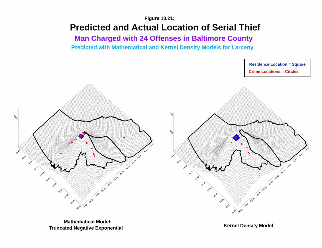
Mathematical Model:Truncated Negative Exponential Kernel Density Model

Predicted and Actual Location of Serial ThiefFigure 10.21:

Man Charged with 24 Offenses in Baltimore CountyPredicted with Mathematical and Kernel Density Models for Larceny

Residence Location = Square

Crime Locations = Circles

10.64

would p roduce even bet t er differen t ia t ion in the m odel t han taking a ll n ight t ime bu rgla r s. However, event ua lly, with fur ther su b-groupin gs there will be insu fficient da ta .

This poin t has been ra ised in a recent deba te. Van Koppen and De Keijser (1997)argued tha t a dis t ance decay fun ction tha t combin ed mult iple inciden t s commit ted by t hesa me individua ls could dist or t the est ima ted r elat ionsh ip compa red t o select ing incident scomm itted by different individua ls.6 Renger t , P iquero and J ones (1999) a rgu ed tha t such adist r ibut ion is never theless m eaningfu l. In our lan gua ge, these a re two differen t su b-gr oups - per sons commit t in g m ult ip le offenses compared to persons commit t in g on ly oneoffense. Combining th ese t wo su b-groups int o a single ca libra t ion da ta set will on ly meantha t the resu lt will ha ve less d ifferen t iat ion in pr edict ion than if the su b-groups weresepa ra ted out .

Actua lly, there is not much d ifference, a t leas t in Ba lt imore County. F rom the41,426 cases, 18,174 were committ ed by persons wh o were only list ed once in t he da tabasewhile 23,251 offenses wer e committ ed by persons wh o were list ed t wo or more t imes (7,802individua ls). Cat egor izing th e 18,174 cr imes as committ ed by ‘single inciden t offender sand the 23,251 cr im es as commit ted by ‘mult ip le in ciden t offenders’, t he densit y d is t ancedecays funct ion s were calcu la ted usin g t he kernel densit y m ethod (Figure 10.22).

The dist r ibut ions a re remarka bly similar . Ther e are some su bt le differences. Theaverage journey t o cr im e t r ip dis t ance made by a sin gle in ciden t offender is lon ger than formult iple in ciden t offender s (4.6 m iles compared to 4.0 miles, on average); the differ en ce ish igh ly sign ificant (p#.0001), pa r t ly because of the ver y la rge sample sizes. H owever , avisu a l inspection of the dist ance decay functions shows t hey a re similar . The singlein ciden t offenders tend to have sligh t ly more t r ips near their home, s ligh t ly fewer fordis tances between about a mile u p t o th ree m iles , and s ligh t ly more longer t r ips . Bu t , thedifferen ces a re n ot very la rge.

There are severa l rea sons for the similar ity. Fir st , some of the ‘single inciden toffenders ’ a re actua lly mult ip le inciden t offenders who have not been charged with otherinciden t s. Second, some of the single inciden t offender s a re in the process of becomingmultiple incident offender s so th eir beh avior is pr obably similar . Third, th ere may not be amajor differ en ce in t r avel pa t t er ns by the number of offens es an individua l comm its,cer t a inly compa red t o the major differences by type of cr ime (see gra ph s a bove). In oth erwords , the dist inction bet ween a sin gle offender crim e t r ip a nd a mult iple offen der crim et r ip is just anoth er su b-group compa r ison and, a pparen t ly, not t ha t impor tan t . Never theles s, it is impor t an t t o choose an appropria t e s ample from which to es t ima te alikely home base loca t ion for a ser ia l offender . The method depends on a sim ila r sample ofoffenders for compar ison .

Sam ple Da ta Se ts for Jou rne y to Crime Rou tine s

Three sa mple da ta set s from Ba ltim ore County ha ve been pr ovided for the journeyto cr ime r out ine. Th e da ta set s a re simula ted and do not represen t rea l da ta . The firs t file- J t cTest 1.dbf, ar e 2000 simu lat ed r obber ies while the second file - J t cTest 2.dbf, ar e 2500

05

1015

2025

10%

8%

6%

4%

2%

0%

Multiple incident offender

Single incident offender

Journey to Crime DistancesFigure 10.22:

Perc

ent o

f all

crim

es

(b

y of

fend

er ty

pe)

Distance from offender's home (miles)

Kernel Density Estimate of Single and Multiple Incident Offenders

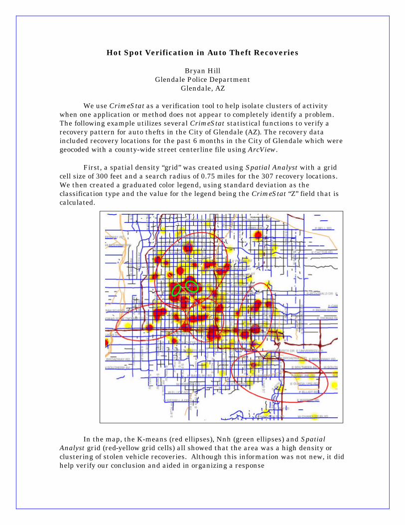
Hot Spot Verification in Auto Theft Recoveries

Bryan Hill Glendale Police Department

Glendale, AZ

We use CrimeStat as a verification tool to help isolate clusters of activity when one application or method does not appear to completely identify a problem. The following example utilizes several CrimeStat statistical functions to verify a recovery pattern for auto thefts in the City of Glendale (AZ). The recovery data included recovery locations for the past 6 months in the City of Glendale which were geocoded with a county-wide street centerline file using ArcView.

First, a spatial density “grid” was created using Spatial Analyst with a grid cell size of 300 feet and a search radius of 0.75 miles for the 307 recovery locations. We then created a graduated color legend, using standard deviation as the classification type and the value for the legend being the CrimeStat “Z” field that is calculated.

In the map, the K-means (red ellipses), Nnh (green ellipses) and Spatial Analyst grid (red-yellow grid cells) all showed that the area was a high density or clustering of stolen vehicle recoveries. Although this information was not new, it did help verify our conclusion and aided in organizing a response

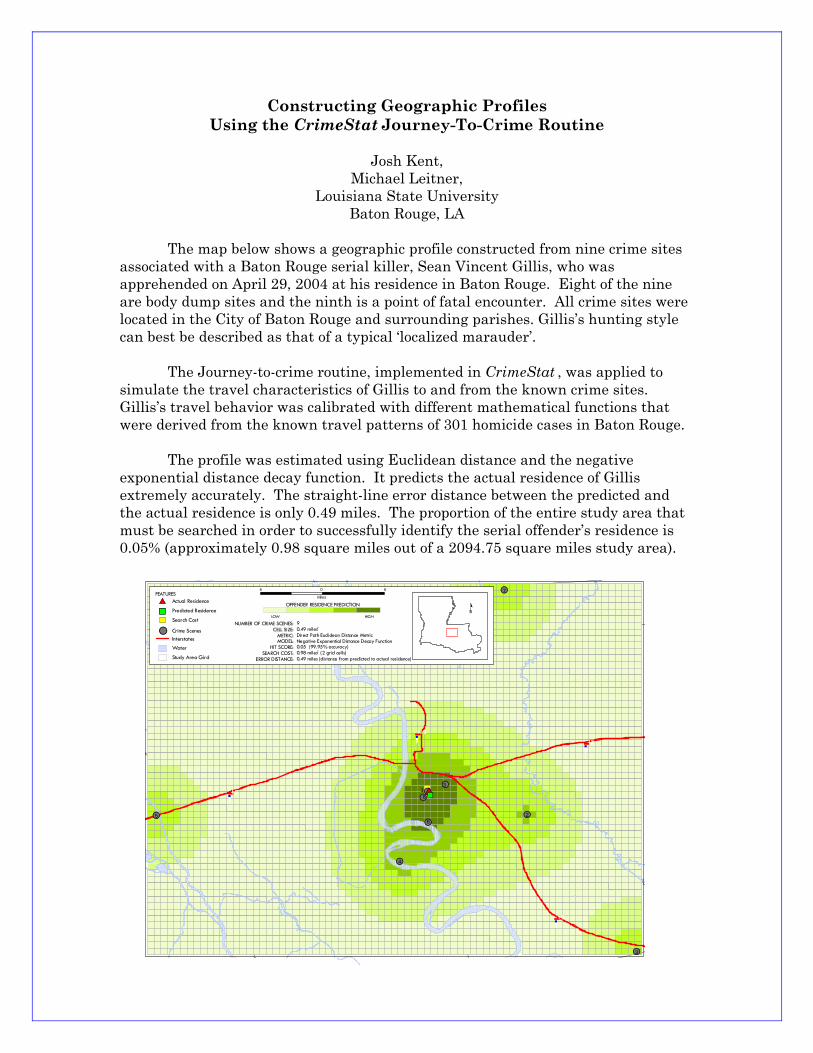
Constructing Geographic Profiles Using the CrimeStat Journey-To-Crime Routine

Josh Kent,

Michael Leitner, Louisiana State University

Baton Rouge, LA

The map below shows a geographic profile constructed from nine crime sites associated with a Baton Rouge serial killer, Sean Vincent Gillis, who was apprehended on April 29, 2004 at his residence in Baton Rouge. Eight of the nine are body dump sites and the ninth is a point of fatal encounter. All crime sites were located in the City of Baton Rouge and surrounding parishes. Gillis’s hunting style can best be described as that of a typical ‘localized marauder’.

The Journey-to-crime routine, implemented in CrimeStat , was applied to simulate the travel characteristics of Gillis to and from the known crime sites. Gillis’s travel behavior was calibrated with different mathematical functions that were derived from the known travel patterns of 301 homicide cases in Baton Rouge.

The profile was estimated using Euclidean distance and the negative exponential distance decay function. It predicts the actual residence of Gillis extremely accurately. The straight-line error distance between the predicted and the actual residence is only 0.49 miles. The proportion of the entire study area that must be searched in order to successfully identify the serial offender’s residence is 0.05% (approximately 0.98 square miles out of a 2094.75 square miles study area).

#S#S

#S

#S#S

#S

#S

#S

#S

$T13

3

25

7

8

6

4

.-,1 0

.-,1 2.-,1 1 0

.-,1 0

%U

%U Predicted Residence$T OFFENDER RESIDENCE PREDICTION

LOW HIGH

#S Crime Scenes

Actual ResidenceFEATURES

Search Cost

Interstates

Water

Study Area Gird

90.49 miles Direct Path Euclidean Distance MetricNegative Exponential Distance Decay Function0.05 (99.95% accuracy)0.98 miles (2 grid cells) 0.49 miles (distance from predicted to actual residence)

2

NUMBER OF CRIME SCENES:CELL SIZE:

METRIC:MODEL:

HIT SCORE:SEARCH COST:

ERROR DISTANCE:

2

8

6 0 6

Miles

10.68

simula ted burgla r ies. Bot h files have coor dina tes for an or igin loca t ion (H om eX, H om eY)and a dest ina t ion loca t ion (IncidentX, Incident Y). User s can use t he ca libra t ion rou t ine t oca lcu la t e t he t r avel d is t ances between the or igins and the des t ina t ions. A th ird dat a set -Ser ial1.dbf, ar e simulat ed incident loca t ions for a ser ial offender . User s can use t he J t cest imat ion rout ine t o iden t ify the likely residence locat ion for th is in dividua l. In runningth is r out ine, a refer en ce grid n eeds t o be overla id (see chapt er 3). For Ba lt imore County,appr opr iat e coordina tes for the lower -left corner a re -76.910 longitude a nd 39.190 la t itudeand for the upper -r igh t corner a re -76.320 longitude a nd 39.720 la t itude.

Draw Crime Trips

The J ourney to Crime modu le includes one u t ility th a t can help visu a lize thepa t t er n before select ing a pa r t icula r est imat ion model. This is a Dr aw Cr ime Tr ips rout inetha t simply dra ws lines between the or igin a nd des t ina t ion of individua l cr ime t r ips. TheX an d Y coordina tes of an origin and destina tion locat ion a re input an d th e rout ine draws aline in ArcView ‘sh p’, MapIn fo ‘mif’, Atlas*GIS ‘bna ’ or Ascii forma t .

F igure 10.23 illust ra tes t he dr awing of the kn own t ravel dist ances for 444 ra pecases for which the residence loca t ion of the rapis t was known. Of the 444 cases, 113 (or25.5%) occur red in the r es idence of th e r apis t . However , for the r em ain ing 331 cases , therape loca t ion was not the residence loca t ion . As seen , m any of t he t r ips a re of qu it e lon gdis tances. Th is would su ggest the u se of an journey to cr ime fun ction tha t has m any t r ipsa t zero dis t ance bu t wit h a more gr adua l decay fu nct ion .

How Accurate are the Methods?

A cr itical ques t ion is how accura te a re these m ethods? The journey to cr ime m odelis ju st tha t , a model. Wh et her it involves u sin g a mathem at ical function or a n em pir ically-der ived one, the a ssumpt ion in the J t c rout ine is t ha t the dist r ibu t ion of inciden t s willprovide in format ion about the home base loca t ion of the offender . In th is sense, it ’s notun like t he wa y most crim e ana lyst s will work wh en they a re t rying to find a ser ia loffender . A typ ica l approach will be to p lot the d is t r ibu t ion of inciden t s and rou t inelysearch a geograph ic ar ea in and a roun d a ser ia l crim e pa t t er n , notin g offenders who ha vean ar res t h ist ory m atchin g case a t t r ibu tes (MO, type wea pon , su spect descr ipt ion, et c.). Because a h igh pr oport ion of offenses a re committ ed with in a sh or t dist ance of offenderresidence’s, t he m et hod can frequen t ly lead t o th eir appreh en sion. But , in doing th ismet hod, the ana lyst s a re not u sin g a soph ist icat ed st a t ist ical m odel.

Tes t S am ple of Se rial Offe n de rs

To explore the accuracy of the appr oach , a sm all sa mple of 50 ser ial offender s wa sisola ted from the da tabase and used as a t a rget sample to test the accuracy of t he methods.The 50 offender s a ccounted for 520 individua l cr ime incident s in the da tabase. To test theJ tc method system at ically, the followin g dis t r ibu t ion wa s selected (ta ble 10.4). The samplewas n ot random, but was selected t o pr odu ce a ba lan ce in t he number of inciden t s

Baltimore County

City of Baltimore

City of BaltimoreBaltimore CountyRape trips

0 10 20 Miles

N

EW

S

Figure 10.23:Journey to Rape Trips

Distance from Residence to Rape Location for 444 Known Offenders

10.70

committ ed by each individu a l an d t o, roughly, app roximate the dist r ibut ion of inciden t s byser ia l offen ders. E ach of the 50 offen ders was isola ted as a sepa ra te file so th a t each couldbe a na lyzed in Crim eS tat.

Ident i fy ing the Crime Type

Each of the 50 offender s wa s cat egor ized by a crim e type. Only two of the offender scommitt ed t he sa me cr ime for a ll their offenses; most committ ed t wo or more differen ttypes of cr imes . Arbitr a r ily, each offender was t yped according to th e cr ime t ype th a the/sh e most frequ ent ly committ ed; in t he two cases wh ere t here wa s a t ie between twocrim e t ypes , the m ost severe wa s selected (i.e., per sona l cr ime over pr oper ty cr ime). WhileI recogn ize tha t there is arbit ra r in ess in the approach , it seemed a pract ica l solu t ion . An yer ror in cat egor izing an offender would be applicable to all th e methods. The cr ime t ypesfor the 50 offen ders approxim ately mir rored the dis t r ibu t ion of inciden t s: la rcen y (29);vehicle theft (7); burgla ry (5); robbery (5); assau lt (2); bank robbery (1); and ar son (1).

Id e n ti fy in g th e Ho m e B as e an d In c id e n t Lo ca ti on s

In the da tabase, each of the offenders was list ed as having a residence loca t ion . F orthe ana lysis, th is was t aken as t he origin loca t ion of th e jour ney t o cr ime t r ip. S imila r ly,the inciden t loca t ion was t aken as t he destina tion for the t r ip. Oper a t iona lly, th e crim e t r ipis t aken as t he dist ance from t he origin locat ion to th e dest ina t ion locat ion . However , it isvery possible tha t some cr im e t r ips actua lly s t a r t ed from other loca t ion s. F ur ther , m any ofthese individu a ls ha ve moved th eir r esidences over t ime; we on ly ha ve the last kn ownresidence in t he da taba se. Un for tuna tely, ther e wa s n o other informat ion in the digita lda tabase t o a llow more accura te ident ifica t ion of the home loca t ion . In oth er words, t heremay be, a nd p robably a re, numer ous er rors in the es t imat ion of th e jour ney t o cr ime t r ip. However , these er rors would be s imilar across a ll met hods a nd should not a ffect theirrela t ive accuracy.

Evaluated Methods

Eleven methods were compared in es t im at in g t he likely residence locat ion of theoffenders . Four of the methods used the J t c rou t ines and seven were s imple spa t ia ldis t r ibu t ion methods (table 10.5).

The mean center and cent er of minim um dist ance are discussed in cha pt er 4. Thecen ter of min imum dis t ance, in pa r t icu la r , is more or les s t he geograph ic cen ter ofdis t r ibu t ion in tha t it ignores the va lu es of par t icu la r loca t ion s; thus, locat ion s tha t a re faraway fr om the clu ster (ext reme va lu es) have no effect on the resu lt . When the cen ter ofminim um dist ance is ca lcu lat ed on a road n etwork in which each segment is weighted byt ravel t im e or speed, t he resu lt is the cen ter of min im um t ravel t im e, t he poin t a t whicht ravel t ime t o each of the inciden t s is m inim ized. The d irectiona l mea n , tr ian gula tedmean , geomet r ic and h armonic means a re discussed in cha pt er 4.

10.71

Ta ble 10 .4

Ser ia l Offende rs Used in Accuracy Evaluat ion

N u m be r o f Cri m e sNum ber of Committed byOffe n de rs Each Pe rson

4 34 44 54 64 74 83 93 103 112 122 132 142 151 161 171 181 191 201 211 221 241 33

_________ _________ 50 520

10.72

Ta ble 10 .5

Com parison Meth ods for Esti m ati n g th e Ho m e Base of a Se ria l Offen de r

Jou rney to Cr ime Methods

Mathemat ica l model for a ll cr imes

Math emat ical model for specific crime type

Kernel dens ity model for a ll cr imes

Kernel den sit y model for specific cr ime t ype

Spat ia l Dis tribut ion Methods

Mean center

Center of min imum d is tance

Cen ter of min imum t r avel t ime (ca lcu lat ed on road n etwork weighted by tr avel t ime)

Directiona l mea n (weight ed) ca lcu lat ed with ‘lower left corner ’as or igin

Tr iangula ted mean

Geomet r ic mean

Harmonic mean

The Test

Each of these eleven methods were run aga in st each of the files crea ted for theser ial offender s. For t he seven ‘means’ (mean center , geomet r ic mean , ha rmonic mean ,d irect iona l mean , t r iangu la ted mean , cen ter of min imum d is tance, cen ter of min imumtravel t im e), t he mean was it self t he best gu ess for the likely residence locat ion of theoffender . F or the four journey t o cr im e funct ion s, t he gr id cell wit h the h ighest likelihoodest ima te was t he best guess for the likely res idence loca t ion of the offender .

Measurem ent o f Error

For each of the 50 offender s, err or was defined a s t he dist ance in m iles between the‘best guess ’ and t he actua l loca t ion . For each offender , th e dist ance between the est ima ted

10.73

home base (the ‘best gu ess’) and the actua l r esidence loca t ion was ca lcu la ted usin g dir ectdis t ances. Table 10.6 presen t s the resu lt s. The da ta show the er ror by m ethod for each ofthe 50 offenders. The th ree r igh t colu mns show the average er ror of a ll methods and theminimum er ror a nd m aximum er rors obta ined by a met hod. The m et hod with theminim um er ror is boldfaced; for some cases , two met hods a re t ied for the minim um. Thebot tom th ree rows show the median er ror , the average er ror and the s t andard devia t ion ofthe er rors for ea ch m et hod across a ll 50 offen ders.

There a re a number of conclu sion s from the resu lt s. F ir st , t he degr ee of precis ionfor any of t hese methods va r ies considerably. The precis ion of the est im ates va ry fr om alow of 0.0466 miles (about 246 feet ) to a h igh of 75.7 miles. The overa ll precis ion of themethods is not very h igh and is h igh ly va r ia ble. There are a number of possible reasons forth is, some of wh ich h ave been discussed a bove. Ea ch of the m et hods produces a sin gleparameter from what is , essen t ia lly, a probabilit y d is t r ibu t ion whereas the dis t r ibu t ion ofmany of t hese in ciden t s a re widely dispersed. F ew of the offenders had such aconcen t r a t ed pa t t ern tha t on ly a single loca t ion was possible. Since these a re p robabilit ydist r ibut ions, not everyone follows t he ‘cen t ra l ten den cy’. Also, some of these offender smay have moved du r ing the per iod in dicated by the inciden t s, t her eby sh iftin g the spa t ia lpa t t ern of inciden t s a nd m akin g it difficu lt t o ident ify th e las t residen ce.

A second conclus ion is tha t , for any one offender , the methods p roduce s imila rresu lt s. F or m any of th e offender s t he differ en ce between the bes t est imate (th e m inimumerror) an d th e worst estimat e (th e maximu m err or) is not great . Thus, the simple meth odsare genera lly a s good (or bad) as the more sophis t ica ted methods.

Thir d, a cross a ll methods, t he cen ter of min im um t ravel t im e, which is ca lcu la ted ona road network (see chapter s 3 and 16), a nd it ’s dis t ance-based ‘cousin ’ - the cen ter ofminimum t ravel t ime, had t he lowest average er ror. Th us, t he approximate geogra ph iccen ter of the d is t r ibu t ion where t r avel t ime to each of the inciden t s was min imal p roducedas good a n est imate a s t he m ore sophist icat ed met hods. H owever , it wa sn ’t pa r t icula r lyclose (3.8415 m iles, on average). The worst method was t he t r iangula ted mea n; it had a naver age er ror of 7.6472 miles . The t r iangula ted mea n is p roduced by vector geomet ry andwill not necessa r ily cap ture the cen ter of the d is t r ibu t ion . Other than th is , there were notgrea t differences. This r einforces t he poin t above th a t the methods a re a ll, more or less,descr ibing the cent ra l ten dency of the dist r ibu t ion . For offender s t ha t don’t live in thecenter of their dis t r ibu t ion, t he er ror of a m et hod will n ecessa ry be h igh .

Lookin g a t each of the 50 offenders, t he methods va ry in their effica cy. Forexa mple, t he J t c kernel fu nct ion for a ll cr im es was the best or t ied for best for 17 of theoffenders, bu t was a lso the worst or t ied for worst for 9. Sim ila r ly, t he J t c kernel fu nct ionfor the specific cr imes was best or t ied for best for 8 of the offender s, but worse for 4. Eventhe most consist en t was best for 4 offender s, but a lso worst for one. On t he other hand,the t r ia ngu la ted mean , which had the worst overa ll er ror , produced the best est im ate for 9of the in dividua ls while it pr oduced t he wor st est imate for 25 of th e in dividua ls. Thus, t het r ian gula ted m ean tends t o be very accura te or very ina ccura te; it h ad t he h ighestva r ia nce, by far .

Table 10.6

Accuracy of Methods for Estimating Serial Offender Residences (N= 50 Serial Offenders)

* Center of Center of *Number Primary * Mean Minimum Minimum Triangulated Geometric Harmonic Jtc Kernel: Jtc Kernel: Jtc Math: Jtc Math: * All Methodsof Crime * Center Distance Travel Time Mean Mean Mean All Crimes Crime Type All Crimes Crime Type * Average Minimum Maximum

Dataset Crimes Type * Error (miles) Error (miles) Error (miles) Error (miles) Error (miles) Error (miles) Error (miles) Error (miles) Error (miles) Error (miles) * Error Error Error------------------- -------------------- --------------------- * ---------------------------- ----------------------------------------------------------------------------------- -------------------------- ----------------------------------------------------- --------------------------- ----------------------- ------------------------- * -------------------- ------------------------------ ---------------------

3A 3 Larceny * 31.5991 32.4477 32.2975 32.4109 31.5995 31.6000 32.7824 32.7880 32.7824 32.7880 * 32.3095 31.5991 32.78803B 3 Larceny * 13.2303 12.1683 12.1207 24.1531 13.2311 13.2319 10.7526 14.4929 10.7526 11.2501 * 13.5384 10.7526 24.15313C 3 Bank robbery * 2.8348 0.9137 0.9588 2.7767 2.8335 2.8322 0.6775 5.8416 0.6775 6.0946 * 2.6441 0.6775 6.09463D 3 Burglary * 2.9733 3.2603 2.6907 6.1013 2.9728 2.9724 4.6038 3.3883 3.3882 3.7931 * 3.6144 2.6907 6.10134A 4 Vehicle theft * 4.2436 4.2670 4.3341 3.8217 4.2436 4.2436 4.2527 4.2364 4.2527 4.2590 * 4.2154 3.8217 4.33414B 4 Larceny * 1.9618 0.3100 0.1158 2.0563 1.9621 1.9623 0.3125 0.2018 0.3125 0.2784 * 0.9473 0.1158 2.05634C 4 Larceny * 4.4733 4.4733 4.5096 4.6789 4.4733 4.4733 4.9681 4.3563 4.2637 4.3563 * 4.5026 4.2637 4.96814D 4 Assault * 0.2925 0.1905 0.0084 0.0466 0.2925 0.2926 0.0703 0.0703 0.0703 0.4560 * 0.1790 0.0084 0.45605A 5 Larceny * 17.3308 16.6459 17.0832 17.8985 17.3292 17.3276 15.9738 17.8655 15.9739 16.4526 * 16.9881 15.9738 17.89855B 5 Larceny * 1.3609 0.2481 0.0565 1.7733 1.3586 1.3564 0.2068 0.6974 0.5140 0.6974 * 0.8269 0.0565 1.77335C 5 Larceny * 2.2458 2.6832 2.7443 16.4518 2.2450 2.2442 2.7886 2.4205 2.7886 3.0922 * 3.9704 2.2442 16.45185D 5 Larceny * 0.9169 0.2250 0.8021 0.2371 0.9171 0.9174 0.1577 0.4267 0.1577 0.4267 * 0.5184 0.1577 0.91746A 6 Larceny * 5.1837 5.2081 5.0644 7.9621 5.1837 5.1837 5.1271 4.8554 4.9393 5.2256 * 5.3933 4.8554 7.96216B 6 Vehicle theft * 1.3720 1.1869 1.1535 0.9625 1.3710 1.3700 3.1126 2.3800 1.3566 2.0831 * 1.6348 0.9625 3.11266C 6 Larceny * 1.3199 0.3157 0.0051 1.7928 1.3192 1.3184 0.2580 0.5272 0.2580 0.5272 * 0.7641 0.0051 1.79286D 6 Larceny * 3.2458 2.3324 3.2838 6.5209 3.2431 3.2405 1.2506 2.6253 1.9718 1.9718 * 2.9686 1.2506 6.52097A 7 Larceny * 3.9023 3.4185 3.1998 2.3176 3.9022 3.9021 2.7419 3.0532 3.1364 3.0532 * 3.2627 2.3176 3.90237B 7 Larceny * 12.4100 9.2973 9.9031 14.8293 12.4107 12.4115 8.5357 8.6148 8.5357 8.8275 * 10.5776 8.5357 14.82937C 7 Burglary * 5.0501 7.1477 6.4354 10.8567 5.0481 5.0460 7.9975 7.9975 7.9975 7.6274 * 7.1204 5.0460 10.85677D 7 Larceny * 2.2686 0.7733 0.3223 75.7424 2.2684 2.2682 0.0892 0.7191 0.0892 0.7191 * 8.5260 0.0892 75.74248A 8 Larceny * 6.0298 6.0165 6.3167 6.2653 6.0264 6.0229 8.4210 6.2962 6.2022 6.1166 * 6.3714 6.0165 8.42108B 8 Larceny * 1.0041 1.1437 1.1458 2.1776 1.0042 1.0042 1.7475 1.3510 1.5298 1.3510 * 1.3459 1.0041 2.17768C 8 Larceny * 1.3059 1.6944 1.6203 1.3684 1.3043 1.3027 2.1513 1.2020 2.1513 1.8707 * 1.5971 1.2020 2.15138D 8 Vehicle theft * 3.5794 2.3780 4.0475 5.5915 3.5809 3.5825 0.5900 1.3340 1.9133 1.3340 * 2.7931 0.5900 5.59159A 9 Robbery * 5.2527 5.7156 5.4565 4.8574 5.2529 5.2532 7.8257 7.1961 6.2520 5.9265 * 5.8989 4.8574 7.82579B 9 Larceny * 8.1923 10.6555 9.9787 6.9916 8.1886 8.1850 12.4578 10.3957 12.4578 12.0514 * 9.9554 6.9916 12.45789C 9 Robbery * 3.7778 3.8454 3.5670 11.0042 3.7758 3.7738 4.9015 5.1862 4.6206 4.3445 * 4.8797 3.5670 11.004210A 10 Larceny * 0.9358 0.5159 0.4822 1.1003 0.9355 0.9353 0.0606 0.3720 0.2601 0.7172 * 0.6315 0.0606 1.100310B 10 Larceny * 2.8581 3.4940 4.8179 14.2219 2.8536 2.8491 6.4051 6.5709 10.3095 6.4758 * 6.0856 2.8491 14.221910C 10 Larceny * 0.8052 0.7251 0.7451 5.5938 0.8050 0.8049 0.9059 0.8404 0.9060 1.2786 * 1.3410 0.7251 5.593811A 11 Vehicle theft * 2.9127 3.2715 3.4493 3.1192 2.9130 2.9134 3.6936 3.4335 3.4282 3.2087 * 3.2343 2.9127 3.693611B 11 Robbery * 0.3250 0.3250 0.2709 0.2513 0.3250 0.3250 0.4235 0.2263 0.4235 0.7011 * 0.3596 0.2263 0.701111C 11 Vehicle theft * 1.2689 1.7157 1.4115 1.4750 1.2709 1.2729 2.8945 0.6984 2.8945 2.2049 * 1.7107 0.6984 2.894512A 12 Larceny * 3.3881 4.2334 4.2640 10.9241 3.3867 3.3852 6.4050 3.2639 5.5843 5.2132 * 5.0048 3.2639 10.924112B 12 Larceny * 0.5562 0.5361 0.4973 2.8003 0.5562 0.5562 0.7897 0.6709 0.7897 0.9631 * 0.8716 0.4973 2.800313A 13 Larceny * 6.3282 7.2857 6.8066 6.0244 6.3248 6.3213 7.6438 7.4607 7.6438 7.9915 * 6.9831 6.0244 7.991513B 13 Assault * 1.4943 1.4943 1.4572 1.5279 1.4944 1.4944 1.6501 1.5954 1.6501 2.0824 * 1.5940 1.4572 2.082414A 14 Larceny * 1.9363 0.8706 0.6681 1.4498 1.9365 1.9368 0.3434 0.6058 0.2596 0.7631 * 1.0770 0.2596 1.936814B 14 Arson * 0.6898 0.3727 0.0251 0.8086 0.6899 0.6900 0.3359 0.3359 0.3359 0.6213 * 0.4905 0.0251 0.808615A 15 Vehicle theft * 0.7282 0.7189 0.8741 0.3362 0.7277 0.7271 0.8155 0.4855 0.8155 1.5128 * 0.7741 0.3362 1.512815B 15 Robbery * 0.4914 0.4914 0.3422 0.8254 0.4914 0.4914 0.6468 0.5693 0.6468 0.6546 * 0.5651 0.3422 0.825416A 16 Vehicle theft * 2.1107 2.0995 2.0555 8.2311 2.1107 2.1107 1.5957 1.6404 2.5911 2.4033 * 2.6949 1.5957 8.231117A 17 Burglary * 1.6484 0.3093 0.1000 1.0227 1.6461 1.6438 0.2879 0.2879 0.2879 0.5268 * 0.7761 0.1000 1.648418A 18 Larceny * 0.6308 0.4196 0.0417 1.0876 0.6329 0.6349 0.2132 0.3383 0.2132 0.6985 * 0.4911 0.0417 1.087619A 19 Larceny * 8.6462 9.4195 9.3665 8.6772 8.6486 8.6511 10.2869 9.2708 9.7022 9.5548 * 9.2224 8.6462 10.286920A 20 Burglary * 6.3520 5.7969 7.4256 28.3094 6.3486 6.3452 0.5934 0.8673 0.5934 0.7945 * 6.3426 0.5934 28.309421A 21 Burglary * 1.2396 0.8861 1.0564 1.2776 1.2393 1.2390 0.5243 0.5243 1.0253 0.4965 * 0.9509 0.4965 1.277622A 22 Larceny * 3.6828 2.6232 2.3597 2.0949 3.6803 3.6777 2.4937 2.8944 2.4937 2.8944 * 2.8895 2.0949 3.682824A 24 Larceny * 1.7959 0.5892 0.9322 2.3033 1.7975 1.7991 0.2658 0.3574 0.4222 0.6587 * 1.0921 0.2658 2.303333A 33 Robbery * 3.9901 5.0481 3.4056 7.2505 3.9940 3.9979 7.9485 7.6939 8.1907 7.9439 * 5.9463 3.4056 8.1907

------------------- -------------------- --------------------- * ---------------------------- ------------------------- ------------------------ -------------------------------- -------------------------- ----------------------------------------------------- --------------------------- ----------------------- ------------------------- * -------------------- ------------------------------ ---------------------Median Error = * 2.5517 2.2159 2.2076 3.4704 2.5509 2.5502 1.9494 2.0102 2.0615 2.1440Mean Error = * 4.0434 3.8441 3.8415 7.6472 4.0429 4.0424 4.0395 4.0305 4.0163 4.1467 *SD Error = * 5.2696 5.4392 5.4619 12.1867 5.2696 5.2695 5.6244 5.6807 5.5961 5.4727 *

10.75

Four th , the m edian er ror is sm aller than the average er ror. Th a t is, t he m edian isthe point a t wh ich 50% of th e cases h ad a sm aller er ror a nd 50% had a la rger er ror. Overa ll, mos t of the cases were found with in a shor ter d is tance than the average wouldindica te. This ind ica tes t ha t severa l cases h ad very la rge err ors wh ereas m ost had sm allerer rors; th a t is, th ey were outliers. Over a ll methods, t he J t c ker nel appr oach for a ll cr imeshad t he lowest median er ror (1.95 m iles). In fact , a ll four J t c methods h ad smaller medianer ror s t han the s imple cen t rograph ic methods. In other words , t hey a re more accu ra t ethan the cent rograph ic met hods m ost of the t ime. The problem in app lying th is logic inpract ice, h owever , is tha t one would not know if t he case bein g s tudied is typ ica l of m ostcases (in which case , the er ror would be r ela t ively small) or wh et her it wa s a n out lier . Inother words, t he median would define a sea rch area tha t capt ured a bout 50% of the cases,bu t would be very wrong in the other 50%. If we could somehow develop a method foriden t ifyin g when a case is ‘typ ica l’ and when it isn’t , increased accuracy will emerge fromthe J t c methods. But , un t il then , th e simple cen ter of minim um t ravel t ime will be th emost accur at e meth od.

Fift h , t he amount of er ror va r ies by t he number of in ciden t s. Table 10.7 belowsh ows t he avera ge err or for each method a s a funct ion of th ree size classes: 1-5 inciden t s;6-9 inciden t s; and 10 or more inciden t s. As can be seen , for ea ch of th e t en met hods, theer ror decreases with increasing number of inciden t s. In th is sense, t he measu red er ror isresponsive to th e sample size from wh ich it is based. I t is, per haps , not surpr isin g tha twith on ly a handful of inciden t s n o method can be very precise.

Sixth , th e relat ive accuracy of each of these m ethods va r ies by sam ple size. Themethod or methods wit h the min im um er ror a re boldfaced. F or a limit ed number ofinciden t s (1-5), the J t c ma them at ical function for a ll cr imes (i.e., the nega t ive exponen t ia lwith the pa rameters from t able 10.5) pr odu ced t he est ima te with the leas t er ror , followedby the J t c kernel funct ion for a ll cr imes ; t he was the th ird bes t . The d ifferences in er rorbetween these were not very grea t . F or the middle ca tegor y (6-9 in ciden t s), t he cen ter ofmin im um dis tance produced the least er ror followed by t he J t c mathemat ica l fu nct ion forthe specific cr ime t ype. For those offender s wh o had committ ed t en or more cr imes , th e J t cker nel function for the specific cr ime t ype pr oduced t he best est imate, followed by t hecen ter of min imum d is tance. The two mathemat ica l funct ions produced the leas t accuracyfor th is sub-gr oup, t hough aga in the differences in er ror a re not very big (2.2 miles for thebest compared to 2.7 miles for the worst ). In other words, on ly wit h a sizeable number ofinciden t s does t he J t c ker nel den sit y approach for specific crim es pr oduce a good est imate. It is bet t er than the other approaches, bu t only sligh t ly bet t er than the sim ple measure ofthe cen ter of minim um dist ance.

S e a rc h Are a

A number of resea rchers have been in teres ted in the concep t of a sea rch a rea for thepolice (Rossmo, 2000; Ca nter , 2003). The concept is tha t the journey t o cr im e method candefine a sm all sea rch a rea wit h in wh ich t her e is a h igher pr obabilit y of find ing theoffender . The average or med ian er ror discussed above can be used to define such a sea rcharea if t r ea ted a s a radius of a circle. While in tu itive, I’m not su re whether th is repr esen t

Table 10.7

Method Estimation Error and Sample Size: Average Error of Method by Number of Incidents (miles)

* Center of Center of Jtc Jtc Jtc Jtc * All MethodsNumber of * Mean Minimum Minimum Triangulated Geometric Harmonic Kernel: Kernel: Math: Math: * Average MinimumIncidents * Center Distance Travel Time Mean Mean Mean All Crime types All Crime types * Error Error-------------- * ----------- ------------------------------------------------------ ---------------- --------------- ----------- ------------------- ----------- ------------------- * ----------------- --------------

3-5 * 6.9553 6.4861 6.4768 9.3672 6.9160 6.9545 6.4622 7.2321 6.3278 6.9954 * 7.0173 6.3278* *

6-9 * 4.2596 4.0753 4.1000 10.6160 4.3331 4.2576 4.4805 4.2489 4.2274 4.2020 * 4.8800 4.0753* *

10+ * 2.3832 2.3149 2.2980 4.8136 2.4575 2.3827 2.4880 2.2176 2.6725 2.6243 * 2.6652 2.2176-------------- * ----------- -------------- -------------------------------------- ---------------- --------------- ----------- ------------------- ----------- ------------------- * ----------------- --------------

10.77

a mea ningfu l st a t ist ic. For exa mple, taking the average er ror of the center of minimumdis tance (3.84 m iles) would produce a sea rch a rea of 46.4 squ are m iles, n ot exa ctly a sm alla rea in which to fin d a ser ia l offender . E ven if we take the media n er ror of 1.94 miles fromthe J t c ker nel a pproach for a ll crim es (1.94 m iles) will st ill pr oduce a sea rch a rea of 11.9square m iles, a nd it would be cor rect only ha lf the t ime

In oth er words , these m et hods a re st ill very impr ecise. Fur ther , the er ror is liableto increase over t ime, r a ther than decrease. With about 50% of th e U.S. popula t ion livingin suburbia (Demograph ia, 1998) and with 90% of Amer ican househ olds owning a t leas tone motor vehicle (U.S. Cens us Bureau , 2000), th e avera ge dista nces t r aveled by offender shas pr obably been in creasing over t ime s ince most types of t r ips h ave also shown increasesin t r avel over t ime. Th is means tha t un less police can find a way to na r row down thesearch a rea consider ably, t he m et hods don’t rea lly help beyond what police intu it ively doanyway, na mely look n ear the dist r ibut ion of the inciden t s committ ed by ser ial offender s.

Ca u ti on a ry No te s

Of cour se, th is is a limited test . It wa s a sm all sa mple (on ly 50 cases) from a sin glejur isdict ion (Baltim ore County). The sa mple wasn ’t even r andomly selected, but chosen toexamine the accu racy by a r ange of s ample s izes . Thus, t he conclusions a re on ly t en ta t ivean d mu st be seen as h ypoth eses for fur th er work . Clearly, more resear ch is needed.

Never theless, t here a re cer ta in cau t ion s tha t must be considered in usin g eit her ofthese journey to cr ime m et hods (the m athem at ical or the em pir ical). Fir st , a sim pletechnique, su ch as t he cen ter of minim um dist ance, ma y be as good a s a more sophist ica tedtechnique. I t doesn’t a lways follow tha t a sophis t ica ted method will p roduce any m oreaccuracy t han a sim ple one. F or the t im e bein g, I would advise cr im e ana lyst s who aret rying t o detect a pa t t ern in the dis t r ibu t ion of the in ciden t s of a ser ia l offender to doexa ctly what they h ave been doing, basica lly looking a t the da ta and m aking a su bject iveguess about where th e offender m ay be residing. The kernel density J tc rout ine needs anadequ a te amoun t of informat ion (i.e, a t lea st 10 in ciden t s) to produce somewh at pr eciseest ima tes. These techniques sh ould be seen for now as r esea rch tools ra ther than asdiagnost ics for ident ifying th e whereabouts of an offender . They ar e just too imprecise andun reliable to depend on, at least u nt il more definitive results ar e obtained.

Second, th ere are other limita t ions t o the technique. The m odel must be ca libra tedfor each in dividua l ju r isdict ion . F ur ther , it must be per iodica lly r e-ca libra ted to accountfor changes in cr ime pa t t erns . For example, in us ing the mathemat ica l model, one cannottake t he pa rameters est ima ted for Balt imore Coun ty (Table 10.3) and a pply th em toanother cit y or if u sin g t he kernel densit y m ethod take the resu lt s found a t one t im e per iodand assume tha t they will r emain in defin it ely. The model is a probabilit y m odel, not aguaran tee of cer ta in ty. It p rovides guesses based on the s imila r ity to other offenders of thesa me t ype of cr ime. In th is sen se, a pa r t icula r ser ia l offen der may not be typical and t hemodel cou ld actua lly or ien t police wrongly if the offender is differen t from the ca libra t ionsa mple. It will t ake insigh t by the invest igat ing officers to know whet her the pa t t er n istyp ica l or not .

10.78

Th ird, a s a theoret ical m odel, the journey to cr ime approach is qu ite simple. It isbased on a dis t r ibu t ion of in ciden t s and an assumed t ravel d is t ance decay fu nct ion . F romthe per spective of modeling the t r avel beha vior of offender s, it is limit ed. As m ent ionedabove, the method does not u t ilize in format ion on the dist r ibut ion of t a rget oppor tun itiesnor does it u t ilize informat ion on t he t r avel mode and r out e t ha t an offender takes. It ispurely a st a t is t ica l m odel. Th e research area of geogr aphic profilin g a t t empts to go beyon dsta t is t ica l descr ip t ion and understand the cogn it ive maps tha t offenders use as well as howthese in ter act with their motives. This is good a nd should clear ly guide fut ure r esea rch. Bu t it has t o be underst ood t ha t the t heory of offender t r avel beh avior is n ot ver y welldeveloped, cer t a in ly compared to other types of t r avel behavior . F ur ther , some types ofcr im e t r ips may n ot even sta r t from an offender ’s residence, bu t may be referenced fromanoth er locat ion , su ch a s veh icle t hefts occur r ing nea r disposa l locat ions. Rout ine activit ytheory would suggest mult ip le or igin s for cr im es (Coh en and Felson, 1979).

Th e exis t ing models of t r avel dem and u sed by t ransport a t ion p lanner s (wh ich h avethem selves been crit icized for being too sim ple) measu re a var iet y of factors t ha t have onlybeen margina lly included in the cr ime t ravel lit era ture - the availability of opport un ities,the concent ra t ion of offender types in cert a in a reas, the mode of t ravel (i.e., au to, bus,wa lk), the specific rou tes t ha t a re taken , th e int eract ion between t ravel t ime a nd t ravelroute, a nd other factors. I t will be im por tan t to in corpora te these elements in to theunderstandin g of jou rney t o cr im e t r ips to bu ild a much more comprehensive theory of h owoffenders opera te. Travel behavior is very complica ted and we need more than a st a t is t ica ldis t ance model t o adequa tely understand it . The next seven chapter s look a t an applica t ionof t r avel demand t heory t o cr ime t ravel.

Also, it ’s n ot clear wh et her knowing a n offender ’s ‘cognit ive map’ will help inpredict ion . There have been no eva lu a t ion s tha t have compared a st r ict ly st a t is t ica lapproach wit h an approach tha t u t ilizes in format ion about the offender as he or sheunderstands the environment . I t cannot be assumed tha t in tegr a t in g in format ion aboutthe percept ion of the environment will a id predict ion . In most t r avel demand forecast stha t t r anspor ta t ion engineers and pla nners make, cognit ive in format ion about theenvironment is not u t ilized except in the defin it ion of t r ip purpose (i.e., wha t the purpose ofthe t r ip was). The models use the actua l t r ips by or igin and dest in a t ion as the basis forformula t ing p red ict ions , not the unders tanding of the t r ip by the ind ividua l. Underst andin g is im por tan t from the viewpoin t of developin g theory or for ways t ocommunica t e with peop le. Bu t , it is not necessa r ily usefu l for pred ict ion . In shor t ,underst andin g and p rediction are n ot t he same t h ing.

On the oth er hand, t he journey to cr ime r out ine, pa r t icula r ly the ker nel densit yappr oach, can be useful for police depar tm ents if used car efu lly. If there are su fficientcases to bu ild an est im ate (i.e., 10 or more in ciden t s), it can provide addit ion a l in format ionto officer s in vest iga t in g a ser ia l offender by r educin g t he number of possible suspect s tha tmight be lin ked to a ser ies of crim es. It can a lso pr ovide some dir ect ion in orien t ing thedeploymen t of officer s a nd det ect ives invest iga t ing wh at appea r to be ser ia l offenses. I tpr ovides gu esses a bout wh er e t he offender might be living, but ba sed on sim ilar it ies wit hprevious offenders for the same type of cr im e. I t ’s not going t o give an exa ct est im ate of

10.79

wh er e an offender is living, but will pr ovide some insigh t s in to which area s t he individua lmight be loca ted. The J t c model should be seen as a supplement to other t echniques, n ot acomplete solu t ion . Like a ll the st a t ist ical t ools in Crim eS tat, it must be u sed ca refully andintelligen t ly. The ph ilosoph y of cr ime ana lysis must a lwa ys be to use a techn ique wit hthought and with a syst emat ic pr ocedu re.

10.80

1. It sh ould a lso be poin ted out tha t the u se of dir ect dis t ances will underest imatet ravel dis t ances pa r t icula r ly if the st reet net work follows a gr id.

2. There are, of course, many other types of mathemat ica l funct ions t ha t can be usedto descr ibe a declin ing likelihood with dis t ance. In fact , ther e a re an infinit enumber of su ch funct ions. However, t he five types of funct ions pr esen ted h ere arecommonly used. We a voided t he inver se dis t ance function because of it s poten t ia l todis tort the likelih ood r ela t ionsh ip.

1f(d) = -------

d ijk

where k is a power (e.g., 1, 2, 2.5). For la rge dis t ances , t h is funct ion can be a usefulapproximat ion of the lessen in g t ravel in teract ion wit h dis t ance. H owever , for shor tdis t ances, it doesn’t work. As the dis t ance between the reference cell loca t ion andan in ciden t loca t ion becomes very small, a pproachin g zero, t hen the likelihoodest im ate becomes very la rge, a pproachin g in fin it y. In fact , for d ij = 0, the fun ction isunsolvable. Since ma ny dista nces bet ween reference cells an d incident s will be zeroor close t o zero, the funct ion becomes u nusa ble.

3. It is actua lly t he in verse of the in verse dis t ance funct ion . If a dis t ance decayfunct ion d rops off p ropor t iona l to the inverse of the d is tance,

Yij = A* 1/d ij

where Yij is t he t r avel likelih ood, A is coefficien t , and d ij is the dis tance from thehome base, then the opposit e - a d ist ance increa se is just the inver se of th is function

1 d ij

Zij = ------------------ = ------------ = B* d ij

A* 1/d ij A

4. There a re severa l sources of er ror associa ted wit h the da ta set . F ir st , t hese recordswere ar rest records p r ior to a t r ial. Un doubt edly, some of the individua ls wereincor rect ly a r res ted . Second , there a re mult ip le offenses . In fact , more than ha lfthe r ecords wer e for individua ls who were lis t ed two or more t imes in the da taba se. The t ravel pa t t ern of repea t offender s m ay be slight ly differen t than for appa rentfirs t -t ime offender s (see figure 10.19). Third, many of these ind ividua ls have livedin mult ip le loca t ions . Cons ider ing tha t many a re young and tha t mos t a re socia llynot well adjust ed, it would be expected tha t these individua ls would have mult iplehomes. Thu s, the dist r ibut ion of inciden t s could reflect multiple home bas es, ra therthan one. Unfor tuna tely, t he da ta we have only gives a sin gle residen t ia l loca t ion ,th e place at wh ich t hey were living when ar rested.

En dn ot e s fo r Ch ap te r 10

10.81

5. If th e coordina te system is projected with th e dista nce units in feet, meters or m iles,then the dist ance between two point s is the hypoten use of a r ight t r iangle usin gEuclidea n geomet ry.

____________________dAB = % (XA - XB)2 + (YA - YB)2 (3.1)

repea twh er e ea ch locat ion is defined by an X and Y coordin a te in feet , met er s, or miles .

If the coordina te syst em is sph er ica l with un its in la t itu des a nd longitudes, t hen thedista nce between t wo points is the Great Circle dista nce. All lat itudes an dlongitudes a re conver ted in to ra dia ns u sin g

2B NRadians (N) = ---------------- (3.2)

360 repea t

2B 8Radians (8) = ---------------- (3.3)

360 repea t

Then , t he dis t ance between the two poin t s is determin ed from

dAB = 2* Arcsin { Sin 2[(NB - NA)/2] + Cos NA*CosNB*Sin 2[(8B - 8A)/2]1 /2 } (3.4)repea t

wit h a ll angles bein g defin ed in radia ns (Snyder , 1987, p . 30, 5-3a ).

6. They a lso argu ed tha t the combin a t ion of in cident s - which they ca lled ‘aggrega t ion ’,would dis tor t the rela t ion sh ip between dis t ance and in cidence likelihood because ofthe ecologica l fa llacy. To m y m in d, t hey a re in cor rect on th is poin t . Da ta on adis t r ibu t ion of inciden t s by dis t ance tr aveled is a n individua l character ist ic and isnot ‘ecologica l’ in a ny way. An ecologica l in ference occurs wh en da ta a re aggregat edwith a grouping var iable (e.g., sta te, county, city, cen su s t r act; see Langbein andLicht man, 1978). A frequen cy dis t r ibu t ion of individua l cr ime t r ip d ist ances is a nin dividua l probabilit y d is t r ibu t ion , s im ila r , for exa mple, t o a dis t r ibu t ion ofindividua ls by height , weight , income or any other character ist ic. Of course, th ereare sub-set s of th e da ta tha t have been aggrega ted (sim ila r to height s of men v.heigh t s of women, for exam ple). Clear ly, iden t ifying sub-groups can make bet t erdis t inctions in a dis t r ibu t ion. But , it is s t ill an individua l pr obabilit y dis t r ibu t ion. Th is doesn ’t pr oduce bias in est imat ing a pa ramet er , on ly var iability. For exampleif a pa r t icula r dis t ance decay function implies tha t 70% of th e offender s live with in ,say, 5 miles of th eir comm itted incident s, then 30% don’t live with in 5 miles. Inother words, because the da ta a re in dividua l level, then a dis t ance decay fu nct ion ,wheth er estimat ed by a m at hema tical or a kern el density model, is an individua lprobabilit y m odel (i.e., an a t t empt to descr ibe the under lyin g dis t r ibu t ion ofin dividua l t r avel d is t ances for journey t o cr im e t r ips).