
Chapter 1. Digital Data Representation and...
54
Chapter 1. Digital Data Representation and Communication
Transcript of Chapter 1. Digital Data Representation and...

Chapter 1. Digital Data Representation and Communication

Introduction
• Digital media is multimedia driven by computers. You can see it, hear it, maybe even touch it, and certainly interact with it.
• What draws most people to a study of digital media is the satisfaction of making something that communicates, entertains, or teaches.
• We consider the topics in digital media work—choosing color modes, compressing files, identifying aliased frequencies, filtering, transforming, and creatively editing.
• We present the mathematical and algorithmic procedures upon which the tools are built.
2

Focus of this Course
• This book is organized around three main media—digital imaging, audio, and video—woven together at the end with multimedia programming.
• Topics in each chapter are motivated by activities done in digital media application programs, but they are presented from a mathematical or conceptual perspective.
3

Chapter Organization
• This chapter covers concepts that are relevant to more than one medium.
• The digitization process of sampling and quantization is introduced, to be revisited in the context of image and sound in later chapters. Analog-to-digital conversion is where it all begins.
• We then move on to fundamentals of data communication and data storage. A survey of compression methods covers concepts relevant to all media.
• We conclude the chapter with an overview of standards and standardization organizations.
4

Analog and digital data
• Analog data• Takes on continuous values• E.g. voice, video
• Digital data• Takes on discrete values• E.g. text, integer
• Converting the continuous phenomena of images, sound, and motion into a discrete representation that can be handled by a computer is called analog-to-digital conversion.
Analog data
Digital data
5

Analog data compared with digital data
• Analog data > digital data
• More information -> more precise and better quality
• Digital data > Analog data
• Size -> transmitted efficiently
• Reliably -> less affected by noise when transmitted
• Computers can only work with digital data.
6

Data and signals
• Usually use digital signals for digital data and analog signals for analog data
• Can use analog signal to carry digital data
• Modem
• Can use digital signal to carry analog data
• Compact Disc audio
7

Analog Signals Carrying Analog and Digital Data
8

Digital Signals Carrying Analog and Digital Data
9

Fourier transform
• Fourier analysis shows that any periodic signal can be decomposed into an infinite sum of sinusoidal waveforms.
• Fourier transform makes it possible to store a complex sound wave in digital form, determine the wave’s frequency components, and filter out components that are not wanted.
10

An example of grayscale image
11

A/D Conversion
• Analog-to-digital conversion requires two steps: sampling and quantization.
• The first step, sampling, chooses discrete points at which to measure a continuous phenomenon (signal).
• For images, the sample points are evenly separated in space. For sound, the sample points are evenly separated in time.
• The number of samples taken per unit time or unit space is called the sampling rate or, alternatively, the resolution.
• The second step, quantization, requires that each sample be represented in a fixed number of bits, called the bit depth. The bit depth limits the precision with which each sample can be represented.
12

Sampling and Aliasing
• Undersampling: sampling rate does not keep up with the rate of change in the signal.
• Aliasing in a digital signal arises from undersampling and results in the sampled discrete signal cannot reconstruct the original source signal.
Audio wave at 637 Hz 637 Hz audio wave sampled at 770 Hz
13

Nyquist theorem
• The Nyquist theorem specifies the sampling rate needed for a given spatial or temporal frequency.
• To guarantee that no aliasing will occur, you must use a sampling rate that is greater than twice the maximal frequency in the signal being sampled.
• Let f be the frequency of a sine wave. Let r be the minimum sampling rate that can be used in the digitization process such that the resulting digitized wave is not aliased. Then the Nyquist frequency r is
r = 2f
14

Quantization
• Let n be the number of bits used to quantize a digital sample. Then the maximum number of different values that can be represented is m = 2n
• Quantization error
15

SNR and SQNR
• Signal-to-noise ratio (SNR) can generally be defined as the ratio of the meaningful content of a signal versus the associated noise.
• In analog data communication, SNR is defined as the ratio of the average power in the signal versus the power in the noise level.
• For a digitized signal, the signal-to-noise ratio is defined as the ratio of the maximum sample value versus the maximum quantization error. This can also be called signal-to-quantization-noise ratio (SQNR)
16

SQNR and Dynamic Range
• Let n be the bit depth of a digitized media, Then the SQNR is
SQNR = 20 log10(2n) (in dB)
• Signal-to-quantization-noise ratio is directly related to dynamic range.
• Dynamic range, informally defined, is the ratio of the largest-amplitude sound (or color, for digital images) and the smallest that can be represented with a given bit depth.
17

Dynamic Range
• With three bits, you have eight colors. You can spread these colors out over a wide range or a narrow range.
• In either case, the dynamic range is the same, dictated by the bit depth, which determines the maximum error possible (resulting from rounding to available colors) relative to the range of colors represented.
18

Data storage
• Table 1.4 Example File Sizes for Digital Image, Audio, And Video
Example Digital Image File Size (without compression):
Example Digital Audio File Size (without compression):
Example Digital Video File Size (without compression):
Resolution: 1024 pixels × 768 pixelsTotal number of pixels: 786,432Color mode: RGBBits per pixel: 24 (i.e., 3 bytes)Total number of bits: 18,874,368(= 2,359,296 bytes)File size: 2.25 MB
Sampling rate: 44.1 kHz (44,100 samples per second)Bit depth: 32 bits per sample (16 for each of two stereo channels) (i.e., 4 bytes)Number of minutes: one minuteTotal number of bits: 84,672,000(= 10,584,000 bytes)File size: 10.09 MB for one minuteData rate of the file: 1.35 Mb/s
rame size: 720 pixels × 480 pixelsBits per pixel: 24Frame rate: ~ 30 frames/sNumber of minutes: one minuteTotal image requirement:14,929,920,000 bitsAudio requirement: 84,672,000 (See column 2.)Total number of bits:15,014,592,000(= 1,876,824,000 bytes)File size: >1.7 GBData rate of the file: 238.65 Mb/s (This calculation doesn’t take chrominance subsampling into account. See Chapter 6 for a discussion of subsampling.) 19

Storage Media and Their Capacity
Storage medium Maximum capacity
Portable Media
CD (Compact Disk) 700 MB
DVD (Digital Versatile Disc or Digital Video Disk), standard one sided
4.7 GB standard; 8.5 GB dual-layered
DVD video or high capacity 17–27 GB
Memory stick or card 8 GB
HD-DVD (High Definition DVD), standard one-sided
15 GB standard; 30 GB dual-layered
Blu-ray Disk 25 GB standard; 50 GB dual-layered
Flash drive 64 GB
Permanent Media
Hard disk drive 1 terabyte (1000 GB)
20

Data Communication
• Analog and digital data communication
• Baseband transmission is used across wire and coaxial cable, but it works well only across relatively short distances. Noise and attenuation cause the signal to degrade as it travels over the communication channel.
Waveform for part of the spoken word “boo” Baseband digital transmission.
21

Modulation
• modulated data transmission (or bandpasstransmission), is based on the observation that a continuously oscillating signal degrades more slowly and thus is better for long distance communication.
• Modulated transmission makes use of a carrier signal on which data are “written.”
• A carrier signal—for example, a beam of light passing through optical fiber or radio waves across free space—that is made to oscillate in a regular sinusoidal pattern at a certain frequency.
22

Modulation Methods
• The three basic methods for modulating a carrier wave are amplitude modulation, frequency modulation, and phase modulation.
• In amplitude modulation, the amplitude of the carrier signal is increased by a fixed amount each time a digital 1 is communicated; in frequency modulation, the frequency is changed; and in phase modulation, the phase is shifted.
23

Summary of analog and digital communication
• Both analog and digital data can be transmitted by means of copper wire, coaxial cable, optical fiber, and free space. The medium of transmission does not determine whether the communication is analog or digital. The form of the data does.
• Digital data can be transmitted by means of a baseband signal or a bandpass (i.e., modulated) signal. The baseband signal uses discrete pulses representing 0s and 1s. The modulated signal uses a carrier frequency and an encoding of data based on periodically altering the frequency, amplitude, or phase of the signal.
• Both analog and digital data can be communicated by means of a modulated signal. A carrier signal can be modulated to contain either analog or digital data.
24

System Bandwidth
• Define: the maximum rate of change of a signal
• Change: first there must be one thing, and thenanother—two different pieces of information
• Example:A transmission system with a bandwidth of 5000 Hz.
Every 1/5000th of a second, this system can communicatetwo things. If one voltage represents a 0 and anotherrepresents a 1, then the system can transmit a 0 and a 1every 1/5000th of a second.
It can transmit 10,000 bits every second.
25
System Bandwidth
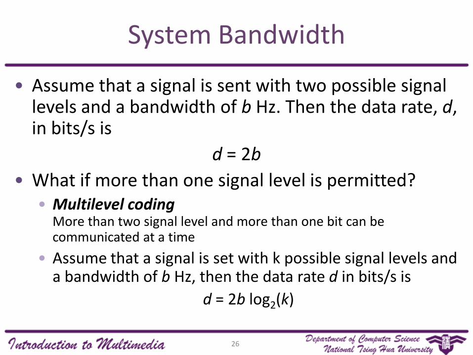
• Assume that a signal is sent with two possible signal levels and a bandwidth of b Hz. Then the data rate, d, in bits/s is
d = 2b
• What if more than one signal level is permitted?• Multilevel coding
More than two signal level and more than one bit can be communicated at a time
• Assume that a signal is set with k possible signal levels and a bandwidth of b Hz, then the data rate d in bits/s is
d = 2b log2(k)
26

Data Rate
• Example for multilevel coding • K=4• Log2(k)=2• Translate 4 bits per
cycle
27

Signal Bandwidth
• For a signal that can be represented as a periodic waveform, let fmax be the frequency of the highest-frequency component and let fmin be the frequency of the lowest-frequency component. Then the width of the signal, w, is
w = fmax − fmin
28

Bandwidth of Communication Channel
• When data is communicated across the airwaves, they are sent along some particular channel, which is a band of frequencies.
• The sender communicates within its designated frequency band, and the receiver tunes to that band to receive the communication.
• The range of frequencies allocated to a band constitutes the bandwidth of a channel.
• Ex. each AM radio station is allocated a bandwidth of 10 kHz. FM radio stations have bandwidths of 200 kHz. Analog television has a bandwidth of about 6 MHz. HDTV requires a bandwidth of approximately 20 MHz.
29
Data Rate
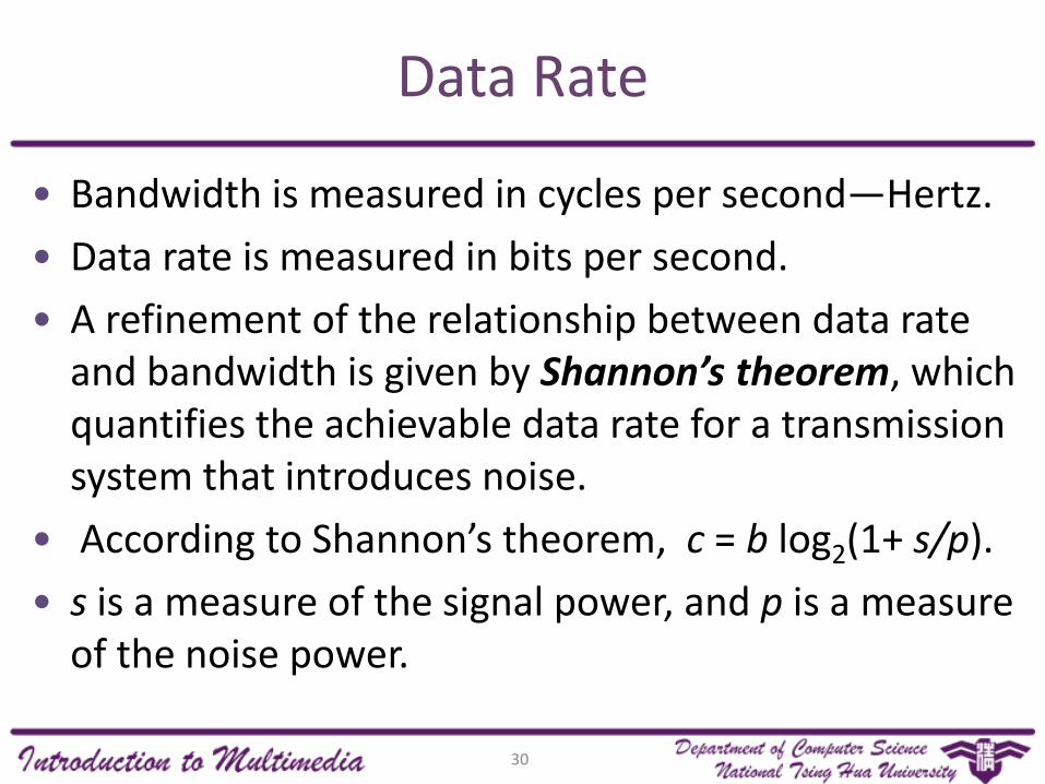
• Bandwidth is measured in cycles per second—Hertz.
• Data rate is measured in bits per second.
• A refinement of the relationship between data rate and bandwidth is given by Shannon’s theorem, which quantifies the achievable data rate for a transmission system that introduces noise.
• According to Shannon’s theorem, c = b log2(1+ s/p).
• s is a measure of the signal power, and p is a measure of the noise power.
30

Baud Rate
• Baud rate: the number of changes in the signal per second, as a property of sending and receiving devices.
• Baud rate is close in meaning to bandwidth as bandwidth relates to digital data communication. The main difference is that baud rate is usually used to refer to sending and receiving devices, whereas bandwidth has other meanings related to frequencies over the airwaves.
• To be precise, baud rate and bit rate are related by the equation d = 2b log2(k).
31

Compression
• Digital media files are usually very large, and they need to be made smaller—compressed
• Without compression• Won’t have storage capacity
• Won’t be able to communicate them across networks without overly taxing the patience of the recipients
• Compression Rate• A file that is reduced by compression to half its original size
50% compression or compression rate is 2:1
• Compression algorithms can be divided into two basic types: lossless compression and lossy compression.
32

Types of compression
• Lossless compression
• No information is lost between the compression and decompression steps
• Reduces the file size to fewer bits
• Method:
Run-Length encoding (RLE)
Entropy encoding
Arithmetic encoding
33

Types of compression
• Lossy compression
• Sacrifice some information which is not important tohuman perception
In image files: subtle changes in color that the eye cannotdetect
In sound files: changes in frequencies that are imperceptibleto the human ear
• Method:
Transform encoding
34

Types of compression
• Dictionary-based methods (e.g. LZW compression) use a look-up table of fixed-length codes.
• Entropy compression uses a statistical analysis of the frequency of symbols and achieves compression by encoding more frequently-occurring symbols with shorter code words.
• Arithmetic encoding is also based on statistical analysis, but encodes an entire file in a single code word rather than creating a separate code for each symbol.
• Adaptive methods gain information about the nature of the file in the process of compressing it, and adapt the encoding to reflect what has been learned at each step.
• Differential encoding is a form of lossless compression that reduces file size by recording the difference between neighboring values rather than recording the values themselves.
35

Run-Length encoding (RLE)
• RLE is a simple example of lossless compression,being used in image compression.
• For example, BMP file optionally use RLE
• Instead of storing value of each pixel, to storenumber pairs (c,n).
• c: grayscale value
• n: how many consecutive pixels have that value
36

Run-Length encoding (RLE)
• Example 1
• Data sequence:
• Encoding result:
• Example 2If one byte is used to represent each n, then the largest value for n is 255. If 1000 consecutive whites exist in the file.
• Encoding result:
255 255 255 255 255 255 242 242 242 242 238 238 238 238 238 238 255 255 255 255
(255, 6), (242, 4), (238, 6), (255, 4)
(255, 255), (255, 255), (255, 255), (255, 235)
37

Run-Length encoding (RLE)
• Example 3
• Data sequence:
• Encoding result:
• RLE is not suitable for those sequence which has fewrepetition.
• Any lossless compression algorithm and for any length file,there will always exist at least one case where the algorithmdoes not reduce the size of an input file of that length.
255 254 253 252 251 250
(255, 1), (244, 1), (253, 1), (252, 1), (251,1), (250,1)
38

Entropy encoding
• Using fewer bits to encode symbols that occurmore frequently, while using more bits forsymbols that occur infrequently
• Shannon’s equation, below, gives us a way ajudging whether our choice of number of bits fordifferent symbols is close to optimal.
•
• S be a string of symbols and pi be the frequency of theith symbol in the string.
39

Entropy encoding
• Applying Shannon’s entropy equation, you candetermine an optimum value for the averagenumber of bits needed to represent each symbol-instance in a string of symbols, based on howfrequently each symbol appears
• Shannon proves that you can’t do better than thisoptimum
40

Example of entropy encoding
•
41

Entropy encoding
• Example 2An image file of 256 pixels and only eight colors
Color FrequencyOptimum Number of
Bits to Encode This ColorRelative Frequency of the Color in the File
Product of Columns 3 and 4
black 100 1.356 0.391 0.530
white 100 1.356 0.391 0.530
yellow 20 3.678 0.078 0.287
orange 5 5.678 0.020 0.111
red 5 5.678 0.020 0.111
purple 3 6.415 0.012 0.075
blue 20 3.678 0.078 0.287
green 3 6.415 0.012 0.075
2.00642

Result of the Shannon-Fano algorithm applied to compression
Color Frequency Code
black 100 00
white 100 10
yellow 20 010
orange 5 0110
red 5 1110
purple 3 0111
blue 20 110
green 3 1111
43

What are the problems?
• Each symbol must be treated individually
• Each symbol has its own code
• Code must be represented in an integral number of bits
44

Arithmetic encoding - 1
• Also beginning with a list of the symbols in theinput file and their frequency of occurrence
• ExampleA file contains 100 pixels in five colors
ColorFrequency Out of Total Number of Pixels in File
Probability Interval Assigned to Symbol
black (K) 40/100 = 0.4 0 – 0.4
white (W) 25/100 = 0.25 0.4 – 0.65
yellow (Y) 15/100 = 0.15 0.65 – 0.8
red (R) 10/100 = 0.1 0.8 – 0.9
blue (B) 10/100 = 0.1 0.9 – 1.0
45

Arithmetic encoding - 2
• Step 1 – Winterval : 0.4 – 0.65
46

Arithmetic encoding - 3
• Step 1 – Winterval : 0.4 – 0.65
• Step 2 – K0.4+0.25*0.4=0.5interval : 0.4 – 0.5
47

Arithmetic encoding - 4
• Step 1 – Winterval : 0.4 – 0.65
• Step 2 – K0.4+0.25*0.4=0.5interval : 0.4 – 0.5
• Step 3 – K0.4+0.1*0.4=0.44interval: 0.4 – 0.44
48

Arithmetic encoding - 5
• Step 1 – Winterval : 0.4 – 0.65
• Step 2 – K0.4+0.25*0.4=0.5interval : 0.4 – 0.5
• Step 3 – K0.4+0.1*0.4=0.44interval: 0.4 – 0.44
• ……
49

Arithmetic decoding - 1
• Final encoding : 0.43137(0.43134+0.4314)/2=0.43137
• 0.43137 fits in the interval assigned to W -> W
• Remove the scaling of W(0.43137-0.4)/0.25=0.12548-> K
• Remove the scaling of K0.12548/0.4=0.3137-> K
• ……
50

Arithmetic decoding - 2
Floating Point Number f, Representing Code
Symbol Whose
Probability Interval
Surrounds f
Low Value for
Symbol’s Probability
Interval
High Value for
Symbol’s Probability
Interval
Size of Symbol’s
Probability Interval
0.43137 W 0.4 0.65 0.25
(0.43137 − 0.4)/(0.65 − 0.4) =0.12548 K 0 0.4 0.4
(0.12548 − 0)/(0.4 − 0) =0.3137 K 0 0.4 0.4
(0.3137 − 0)/(0.4 − 0) =0.78425 Y 0.65 0.8 0.15
(0.78425 − 0.65)/(0.8 − 0.65) =0.895 R 0.8 0.9 0.1
(0.895 − 0.8)/(0.9 − 0.8) =0.95 B 0.9 1.0 0.1
51

Transform Encoding - 1
• Lossy methods are often based upon transformencoding
• Most commonly used transforms in digital media• Discrete cosine transform (DCT)
• Discrete Fourier transform (DFT)
• No information is lost in the DCT or DFT. When atransform is used, it becomes possible to discardredundant or irrelevant information in later steps,thus reducing the digital file size. This is the lossypart of the process.
52

Transform Encoding - 2
• Discrete cosine transform
Origin image (8x8) Discrete cosine transform
53
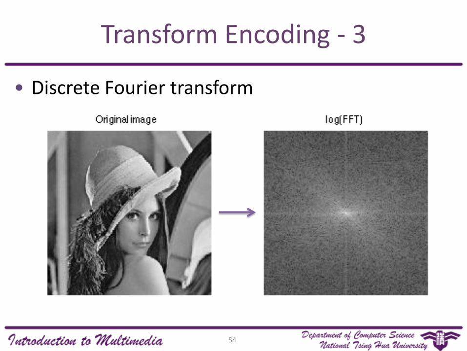
Transform Encoding - 3
• Discrete Fourier transform
54


![[PPT]Classification of Digital Computers & Applications … files/session - 2 Classification... · Web viewClassification of Digital Computers & Applications of Computers Classification](https://static.fdocuments.net/doc/165x107/5ac22b067f8b9ae45b8e3b73/pptclassification-of-digital-computers-applications-filessession-2-classificationweb.jpg)


