Digital Image Representation - nets.rwth-aachen.de · • Digital image representation ... Chapter...

Lehrstuhl für Informatik 4

Kommunikation und verteilte Systeme

Chapter 2.2: Images and Graphics

2.2: Images and Graphics• Digital image representation

• Image formats and color models• JPEG, JPEG2000• Image synthesis and graphics

systems

Chapter 2: Representation of Multimedia Data• Audio Technology

• Images and Graphics• Video Technology

Chapter 3: Multimedia Systems –Communication Aspectsand Services

Chapter 4: Multimedia Systems –Storage Aspects



Page 2Chapter 2.2: Images and Graphics

A digital image is a spatial representation of an object(2D, 3D scene or another image - real or virtual)

Definition of “digital image”:Let I, J, K ⊆ Z be a finite interval. Let G ⊂ N0 with |G| < ∞ be the grey scale level / color depth (intensity value of a picture element = a pixel) of the image.

(1) A 2D-image is a function f: I × J → G(2) A 3D-image is a function f: I × J × K → G

(3) If G = {0,1}, the function is a binary (or bit) image, otherwise it is a pixel image

The Resolution depends on the size of I and J (and K) and describes the number of pixels per row resp. column.

Example

To display a 525-line television picture (NTSC) without noticeable degradation with a Video Graphics Array (VGA) video controller, 640x480 pixels and 256 discrete grey levels give an array of 307.200 8-bit numbers and a total of 2.457.600 bit.

Digital Image Representation




An Image Capturing Format is specified by:

spatial resolution (pixel x pixel) and color encoding (bits per pixel)

Example: captured image of a DVD video with 4:3 picture size:

spatial resolution: 768 x 576 pixelcolor encoding: 1-bit (binary image), 8-bit (color or grayscale),

24-bit (color-RGB)

Image Representation

An Image Storing Format is a 2-dimensional array of values representing the image in a bitmap or pixmap, respectively. Also called raster graphics. The data of the fields of a bitmap is a binary digit, data in a pixmap may be a collection of:

• 3 numbers representing the intensities of red, green, and blue components of the color

• 3 numbers representing indices to tables of red, green and blue intensities• Single numbers as index to a table of color triples

• Single numbers as index to any other data structures that represents a color / colorsystem

Further properties can be assigned with the whole image: width, height, depth, version, etc.




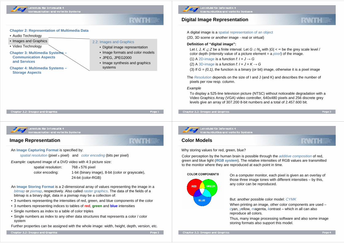
Color Models

Why storing values for red, green, blue?

Color perception by the human brain is possible through the additive composition of red, green and blue light (RGB system). The relative intensities of RGB values are transmitted to the monitor where they are reproduced at each point in time.

On a computer monitor, each pixel is given as an overlay of those three image tones with different intensities – by this, any color can be reproduced.

But: another possible color model: CYMK

When printing an image, other color components are used –cyan, yellow, magenta, kontrast – which in all can also reproduce all colors.Thus, many image processing software and also some image storing formats also support this model.




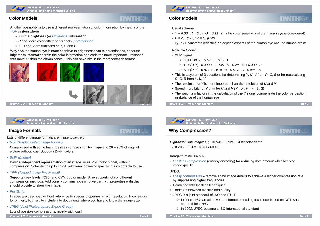
Another possibility is to use a different representation of color information by means of the YUV system where

• Y is the brightness (or luminance) information• U and V are color difference signals (chrominance)

• Y, U and V are functions of R, G and BWhy? As the human eye is more sensitive to brightness than to chrominance, separate brightness information from the color information and code the more important luminance with more bit than the chrominance – this can save bits in the representation format.

Color Models




Usual scheme:

• Y = 0.30 · R + 0.59 ·G + 0.11 · B (the color sensitivity of the human eye is considered)• U = c1 · (B-Y); V = c2 ·(R-Y)

• c1 , c2 = constants reflecting perception aspects of the human eye and the human brain!

Possible Coding:• YUV signal

� Y = 0.30 R + 0.59 G + 0.11 B� U = (B-Y) · 0.493 = - 0.148 · R - 0.29 · G + 0.439 · B� V = (R-Y) · 0.877 = 0.614 · R - 0.517 · G - 0.096 · B

• This is a system of 3 equations for determining Y, U, V from R, G, B or for recalculating R, G, B from Y, U, V

• The resolution of Y is more important than the resolution of U and V

• Spend more bits for Y than for U and V (Y : U : V = 4 : 2 : 2)• The weighting factors in the calculation of the Y signal compensate the color perception

misbalance of the human eye

Color Models




Image FormatsLots of different image formats are in use today, e.g.• GIF (Graphics Interchange Format)

Compressed with some basic lossless compression techniques to 20 – 25% of original picture without loss. Supports 24-bit colors.

• BMP (Bitmap)

Devide-independent representation of an image: uses RGB color model, without compression. Color depth up to 24-bit, additional option of specifying a color table to use.

• TIFF (Tagged Image File Format)Supports grey levels, RGB, and CYMK color model. Also supports lots of different compression methods. Additionally contains a descriptive part with properties a displayshould provide to show the image.

• PostScriptImages are described without reference to special properties as e.g. resolution. Nice feature for printers, but hard to include into documents where you have to know the image size...

• JPEG (Joint Photographics Expert Group)Lots of possible compressions, mostly with loss!




Why Compression?

High-resolution image: e.g. 1024×768 pixel, 24 bit color depth→ 1024·768·24 = 18.874.368 bit

Image formats like GIF:

• Lossless compression (entropy encoding) for reducing data amount while keeping image quality

JPEG: • Lossy compression – remove some image details to achieve a higher compression rate

by suppressing higher frequencies

• Combined with lossless techniques• Trade-Off between file size and quality

• JPEG is a joint standard of ISO and ITU-T� In June 1987, an adaptive transformation coding technique based on DCT was

adopted for JPEG

� In 1992, JPEG became a ISO international standard




JPEG

Implementation

• Independent of image size• Applicable to any image and pixel aspect ratio

Color representation

• JPEG applies to color and grey-scaled still images

Image content• Of any complexity, with any statistical characteristics

Properties of JPEG• State-of-the-art regarding compression factor and image quality

• Run on as many available standard processors as possible• Compression mechanisms are available as software-only packages or together with

specific hardware support - use of specialized hardware should speed up image decompression

• Encoded data stream has a fixed interchange format • Fast coding is also used for video sequences: Motion JPEG




How could We compress?

Entropy encoding

� Data stream is considered to be a simple digital sequence without semantics� Lossless coding, decompression process regenerates the data completely

� Used regardless of the media‘s specific characteristics� Examples: Run-length encoding, Huffman encoding, Arithmetic encoding

Source encoding� Semantics of the data are taken into account

� Lossy coding (encoded data are not identical with original data) � Degree of compression depends on the data contents

� Example: Discrete Cosine Transformation (DCT) as transformation technique of the spatial domain into the two-dimensional frequency domain

Hybrid encoding

� Used by most multimedia systems� Combination of entropy and source encoding

� Examples: JPEG, MPEG, H.261




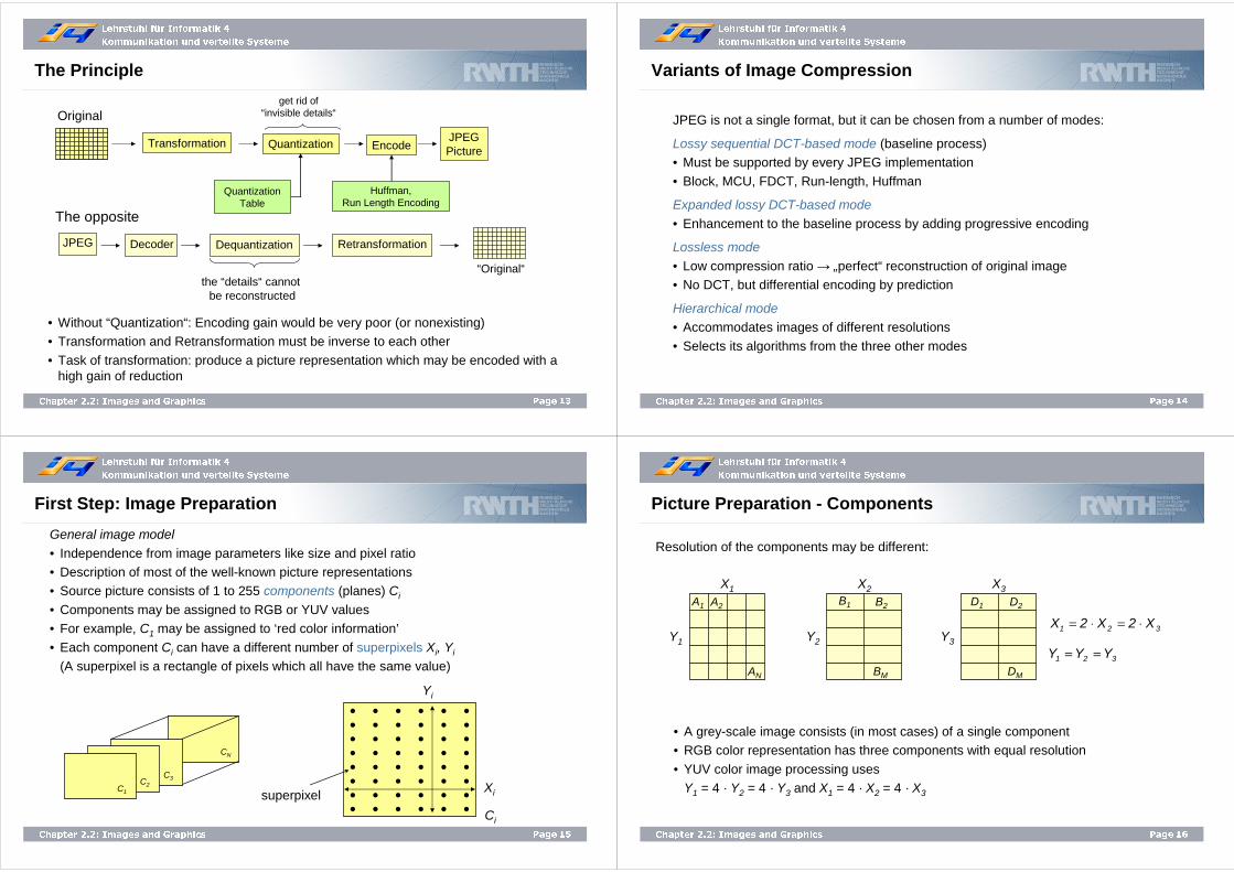
Compression Steps in JPEG

ImagePreparation

Pixel

Quantization(approxima-tion of real numbers by

rational numbers)

Block, MCU

Image Processing

Predictor

DCT

Entropy Encoding

Run-length

Huffman

Arithmetic

UncompressedImage

CompressedImage

MCU: Minimum Coded UnitDCT: Discrete Cosine Transform





Image Preparation• Analog-to-digital conversion

• Image division into blocks of N×N pixels• Suitable structuring and ordering of image information

Image Processing - Source Encoding• Transformation from time to frequency domain using DCT

• In principle no compression itself – but computation of new coefficients as input forcompression process

Quantization

• Mapping of real numbers into rational numbers (approximation)• A certain loss of precision will in general be unavoidable

Entropy Encoding• Lossless compression of a sequential digital data stream




The Principle

• Without “Quantization“: Encoding gain would be very poor (or nonexisting) • Transformation and Retransformation must be inverse to each other

• Task of transformation: produce a picture representation which may be encoded with a high gain of reduction

Original

Transformation Quantization

get rid of“invisible details“

QuantizationTable

Encode

Huffman,Run Length Encoding

JPEGPicture

The opposite

JPEG Decoder Dequantization

the “details“ cannotbe reconstructed

Retransformation

“Original“




Variants of Image Compression

JPEG is not a single format, but it can be chosen from a number of modes:

Lossy sequential DCT-based mode (baseline process)• Must be supported by every JPEG implementation

• Block, MCU, FDCT, Run-length, Huffman

Expanded lossy DCT-based mode

• Enhancement to the baseline process by adding progressive encoding

Lossless mode

• Low compression ratio → „perfect“ reconstruction of original image• No DCT, but differential encoding by prediction

Hierarchical mode• Accommodates images of different resolutions

• Selects its algorithms from the three other modes




First Step: Image Preparation

General image model

• Independence from image parameters like size and pixel ratio • Description of most of the well-known picture representations• Source picture consists of 1 to 255 components (planes) Ci

• Components may be assigned to RGB or YUV values• For example, C1 may be assigned to ‘red color information’

• Each component Ci can have a different number of superpixels Xi, Yi

(A superpixel is a rectangle of pixels which all have the same value)

Yi

Ci

Xisuperpixel• • •• • •• • •• • •• • •• • •• • •• • •• • •• • •• • •• • •• • •• • •• • •• • •

CN

C3C2C1




Picture Preparation - Components

Resolution of the components may be different:

A1

AN

A2

X1

Y1

B1

BM

B2

X2

Y2

D1

DM

D2

X3

Y3

1 2 3

1 2 3

X 2 X 2 X

Y Y Y

= ⋅ = ⋅

= =

• A grey-scale image consists (in most cases) of a single component• RGB color representation has three components with equal resolution

• YUV color image processing usesY1 = 4 · Y2 = 4 · Y3 and X1 = 4 · X2 = 4 · X3




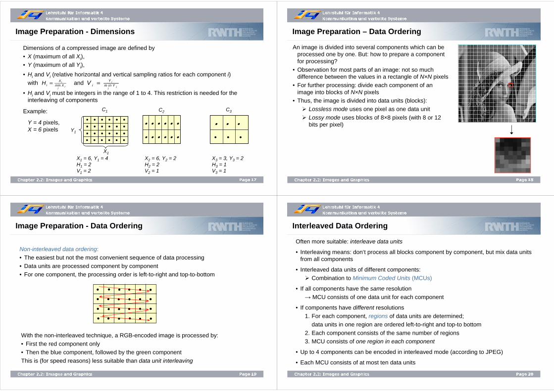
Image Preparation - Dimensions

Dimensions of a compressed image are defined by

• X (maximum of all Xi),• Y (maximum of all Yi),

• Hi and Vi (relative horizontal and vertical sampling ratios for each component i) with and

• Hi and Vi must be integers in the range of 1 to 4. This restriction is needed for the interleaving of components

Example:

Y = 4 pixels, X = 6 pixels

X1 = 6, Y1 = 4H1 = 2V1 = 2

i

jj

Xi min XH = i

jj

Yi m in YV =

• • •

X3 = 3, Y3 = 2H3 = 1V3 = 1

X2 = 6, Y2 = 2H2 = 2V2 = 1

C2

• • •

C3

• • • • • •

• • • • • •

X1

••••

••••

••••

••••

••••

••••

C1

Y1




Image Preparation – Data Ordering

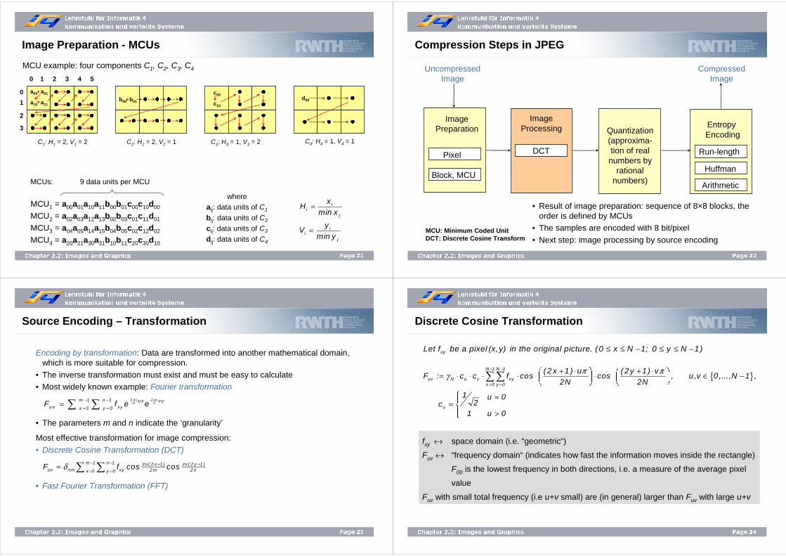
An image is divided into several components which can be processed one by one. But: how to prepare a component for processing?

• Observation for most parts of an image: not so much difference between the values in a rectangle of N×N pixels

• For further processing: divide each component of an image into blocks of N×N pixels

• Thus, the image is divided into data units (blocks):� Lossless mode uses one pixel as one data unit

� Lossy mode uses blocks of 8×8 pixels (with 8 or 12 bits per pixel)




Image Preparation - Data Ordering

Non-interleaved data ordering:• The easiest but not the most convenient sequence of data processing

• Data units are processed component by component• For one component, the processing order is left-to-right and top-to-bottom

•• • • • •• • • • • •

•

•••

•

•

•

•

•

•

•

•

With the non-interleaved technique, a RGB-encoded image is processed by:

• First the red component only• Then the blue component, followed by the green component

This is (for speed reasons) less suitable than data unit interleaving




Interleaved Data Ordering

Often more suitable: interleave data units

• Interleaving means: don‘t process all blocks component by component, but mix data units from all components

• Interleaved data units of different components:

� Combination to Minimum Coded Units (MCUs)

• If all components have the same resolution

→ MCU consists of one data unit for each component

• If components have different resolutions

1. For each component, regions of data units are determined;data units in one region are ordered left-to-right and top-to bottom

2. Each component consists of the same number of regions3. MCU consists of one region in each component

• Up to 4 components can be encoded in interleaved mode (according to JPEG)

• Each MCU consists of at most ten data units




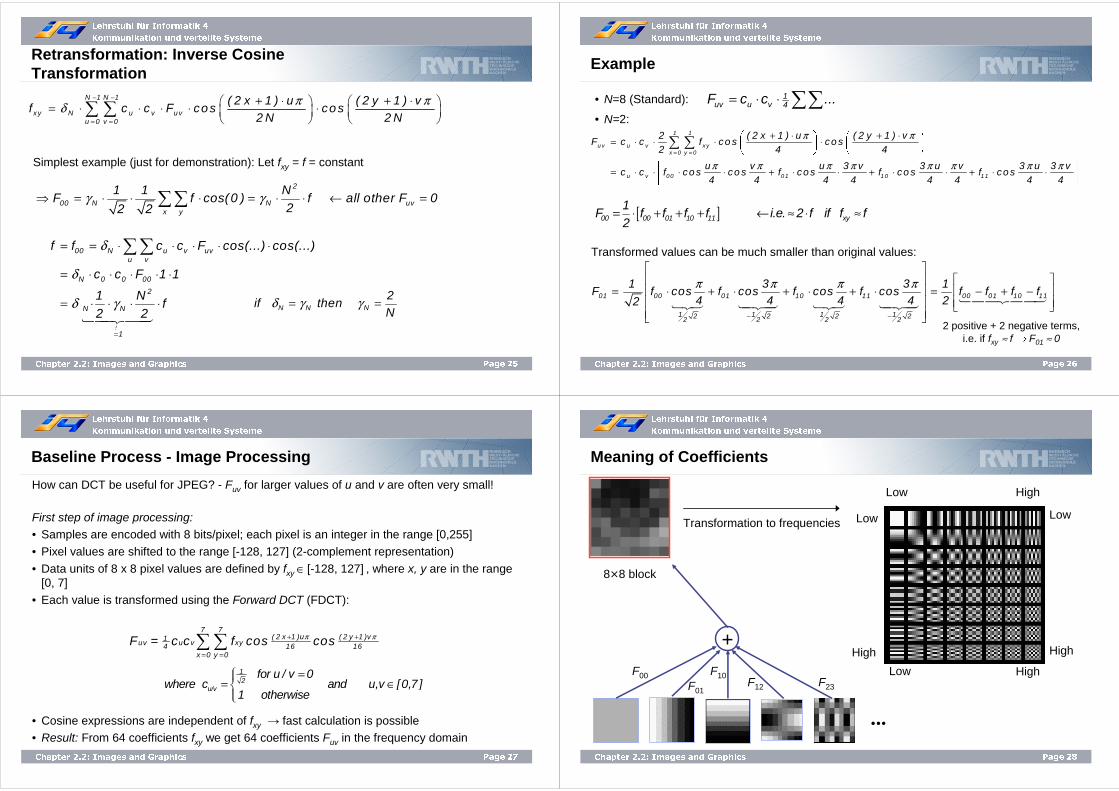
Image Preparation - MCUs

0 1 2 3 4 5

0

1

2

3

MCU example: four components C1, C2, C3, C4

a00 a01

a10 a11

� �

� �

� �

� �

� �

� �

� �

� �

� �

� �

b00 b01 � � � �

� ��

C2: H2 = 2, V2 = 1C1: H1 = 2, V1 = 2

c00

c10

�

�

�

�

�

�

�

�

�

�

C3: H3 = 1, V3 = 2 C4: H4 = 1, V4 = 1

d00 � �

��

MCUs: 9 data units per MCU

MCU1 = a00a01a10a11b00b01c00c10d00

MCU2 = a02a03a12a13b02b03c01c11d01

MCU3 = a04a05a14a15b04b05c02c12d02

MCU4 = a20a21a30a31b10b11c20c30d10

ii

j

ii

j

xH

min x

yV

min y

=

=

whereaij: data units of C1

bij: data units of C2

cij: data units of C3

dij: data units of C4





ImagePreparation

Pixel


rational numbers)

Block, MCU

Image Processing Entropy

Encoding

Run-length

Huffman

Arithmetic

UncompressedImage

CompressedImage

• Result of image preparation: sequence of 8×8 blocks, the order is defined by MCUs

• The samples are encoded with 8 bit/pixel

• Next step: image processing by source encoding

DCT





Source Encoding – Transformation

Encoding by transformation: Data are transformed into another mathematical domain, which is more suitable for compression.

• The inverse transformation must exist and must be easy to calculate• Most widely known example: Fourier transformation

• The parameters m and n indicate the ‘granularity’

Most effective transformation for image compression:

• Discrete Cosine Transformation (DCT)

• Fast Fourier Transformation (FFT)

2 i 2 im n

m 1 n 1 u x vyu v xyx 0 y 0

F f e eπ π− −

= == ∑ ∑

m 1 n 1 u( 2 x 1 ) v ( 2 y 1 )uv nm xy 2 m 2 nx 0 y 0

F f cos cosπ πδ − − + += =

= ∑ ∑




Discrete Cosine Transformation

xyLet f be a pixel (x,y) in the original picture. (0 x N 1; 0 y N 1)≤ ≤ − ≤ ≤ −

{ }N 1 N 1

uv N u v xyx 0 y 0

u

( 2 x 1 ) u ( 2 y 1 ) vF : c c f cos cos , u ,v 0,...,N 1 ,

2N 2N

1 u 02 c

1 u 0

π πγ− −

= =

+ ⋅ + ⋅⎛ ⎞ ⎛ ⎞= ⋅ ⋅ ⋅ ⋅ ⋅ ∈ −⎜ ⎟ ⎜ ⎟⎝ ⎠ ⎝ ⎠

⎧ =⎪= ⎨⎪ >⎩

∑∑

fxy ↔ space domain (i.e. “geometric“)

Fuv ↔ “frequency domain“ (indicates how fast the information moves inside the rectangle)

F00 is the lowest frequency in both directions, i.e. a measure of the average pixel

value

Fuv with small total frequency (i.e u+v small) are (in general) larger than Fuv with large u+v




Retransformation: Inverse Cosine Transformation

N 1 N 1

xy N u v u vu 0 v 0

( 2 x 1 ) u ( 2 y 1 ) vf c c F co s co s

2 N 2 Nπ πδ

− −

= =

+ ⋅ + ⋅⎛ ⎞ ⎛ ⎞= ⋅ ⋅ ⋅ ⋅ ⋅⎜ ⎟ ⎜ ⎟⎝ ⎠ ⎝ ⎠

∑ ∑

2

00 N N uvx y

1 1 NF f cos(0 ) f all other F 0

22 2γ γ⇒ = ⋅ ⋅ ⋅ = ⋅ ⋅ ← =∑∑

N N N

2if then

Nδ γ γ= =

!

00 N u v uvu v

N 0 0 00

2

N N

1

f f c c F cos(...) cos(...)

c c F 1 1

1 Nf

2 2

δ

δ

δ γ

=

= = ⋅ ⋅ ⋅ ⋅ ⋅

= ⋅ ⋅ ⋅ ⋅ ⋅

= ⋅ ⋅ ⋅ ⋅

∑∑

��

Simplest example (just for demonstration): Let fxy = f = constant




Example

• N=8 (Standard):

• N=2:

1uv u v 4F c c ...= ⋅ ⋅ ∑∑

1 1

u v u v xyx 0 y 0

u v 00 0 1 1 0 1 1

2 ( 2 x 1 ) u ( 2 y 1 ) vF c c f co s co s

2 4 4

u v u 3 v 3 u v 3 u 3 vc c f co s co s f co s f co s f co s

4 4 4 4 4 4 4 4

π π

π π π π π π π π= =

+ ⋅ + ⋅⎛ ⎞ ⎛ ⎞= ⋅ ⋅ ⋅ ⋅⎜ ⎟ ⎜ ⎟⎝ ⎠ ⎝ ⎠

⎡ ⎤= ⋅ ⋅ ⋅ ⋅ + ⋅ ⋅ + ⋅ ⋅ + ⋅ ⋅⎢ ⎥⎣ ⎦

∑ ∑

[ ]00 00 01 10 11 xy

1F f f f f i.e. 2 f if f f

2= ⋅ + + + ← ≈ ⋅ ≈

01 00 01 10 11 00 01 10 11

1 1 1 12 2 2 22 2 2 2

1 3 3 1F f cos f cos f cos f cos f f f f

4 4 4 4 22

π π π π

− −

⎡ ⎤⎢ ⎥ ⎡ ⎤⎢ ⎥ ⎢ ⎥= ⋅ + ⋅ + ⋅ + ⋅ = − + −⎢ ⎥ ⎢ ⎥⎣ ⎦⎢ ⎥⎣ ⎦

��

2 positive + 2 negative terms,i.e. if fxy ≈ f ⇒ F01 ≈ 0

Transformed values can be much smaller than original values:




Baseline Process - Image Processing

First step of image processing:• Samples are encoded with 8 bits/pixel; each pixel is an integer in the range [0,255]

• Pixel values are shifted to the range [-128, 127] (2-complement representation)

• Data units of 8 x 8 pixel values are defined by fxy ∈ [-128, 127] , where x, y are in the range [0, 7]

• Each value is transformed using the Forward DCT (FDCT):

7 7( 2 x 1 )u ( 2 y 1 )v1

uv u v xy4 16 16x 0 y 0

F = c c f cos cosπ π+ +

= =∑∑

12

u/v

for u / v 0where c and u,v [0,7 ]

1 otherwise

=⎧⎪= ∈⎨⎪⎩

• Cosine expressions are independent of fxy → fast calculation is possible• Result: From 64 coefficients fxy we get 64 coefficients Fuv in the frequency domain

How can DCT be useful for JPEG? - Fuv for larger values of u and v are often very small!




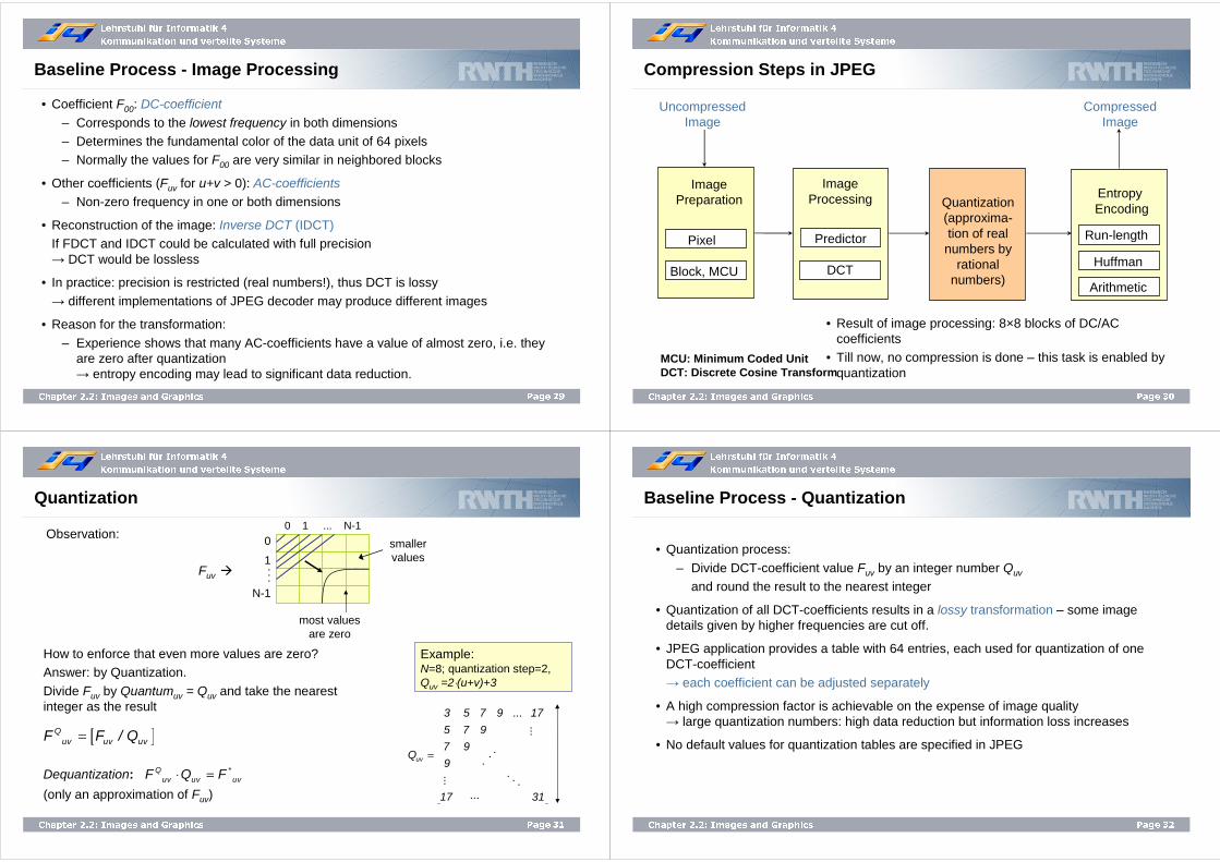
Meaning of Coefficients

Low

Low

High

High

Low

High

HighLow

8×8 block

Transformation to frequencies

+

...

F00

F01

F10F12 F23




Baseline Process - Image Processing

• Coefficient F00: DC-coefficient

– Corresponds to the lowest frequency in both dimensions– Determines the fundamental color of the data unit of 64 pixels– Normally the values for F00 are very similar in neighbored blocks

• Other coefficients (Fuv for u+v > 0): AC-coefficients– Non-zero frequency in one or both dimensions

• Reconstruction of the image: Inverse DCT (IDCT)If FDCT and IDCT could be calculated with full precision → DCT would be lossless

• In practice: precision is restricted (real numbers!), thus DCT is lossy

→ different implementations of JPEG decoder may produce different images

• Reason for the transformation:

– Experience shows that many AC-coefficients have a value of almost zero, i.e. they are zero after quantization → entropy encoding may lead to significant data reduction.





ImagePreparation

Pixel


rational numbers)

Block, MCU

Image Processing

Predictor

EntropyEncoding

Run-length

Huffman

Arithmetic

UncompressedImage

CompressedImage

• Result of image processing: 8×8 blocks of DC/AC coefficients

• Till now, no compression is done – this task is enabled by quantization

DCT





Quantization

How to enforce that even more values are zero?Answer: by Quantization.

Divide Fuv by Quantumuv = Quv and take the nearest integer as the result

[ ]Quv uv uvF F / Q=

Q *uv uv uvF Q F⋅ =

uv

3 5 7 9 ... 17

5 7 9

7 9Q

9

17 31

⎡ ⎤⎢ ⎥⎢ ⎥⎢ ⎥

= ⎢ ⎥⎢ ⎥⎢ ⎥⎢ ⎥⎢ ⎥⎣ ⎦...

...

...

. . .

.. .

Example:N=8; quantization step=2, Quv =2⋅(u+v)+3

Fuv �

smaller values

most values are zero

0 1 ... N-1

0

1...N-1

Observation:

Dequantization:

(only an approximation of Fuv)




Baseline Process - Quantization

• Quantization process:

– Divide DCT-coefficient value Fuv by an integer number Quv

and round the result to the nearest integer

• Quantization of all DCT-coefficients results in a lossy transformation – some image details given by higher frequencies are cut off.

• JPEG application provides a table with 64 entries, each used for quantization of one DCT-coefficient → each coefficient can be adjusted separately

• A high compression factor is achievable on the expense of image quality→ large quantization numbers: high data reduction but information loss increases

• No default values for quantization tables are specified in JPEG




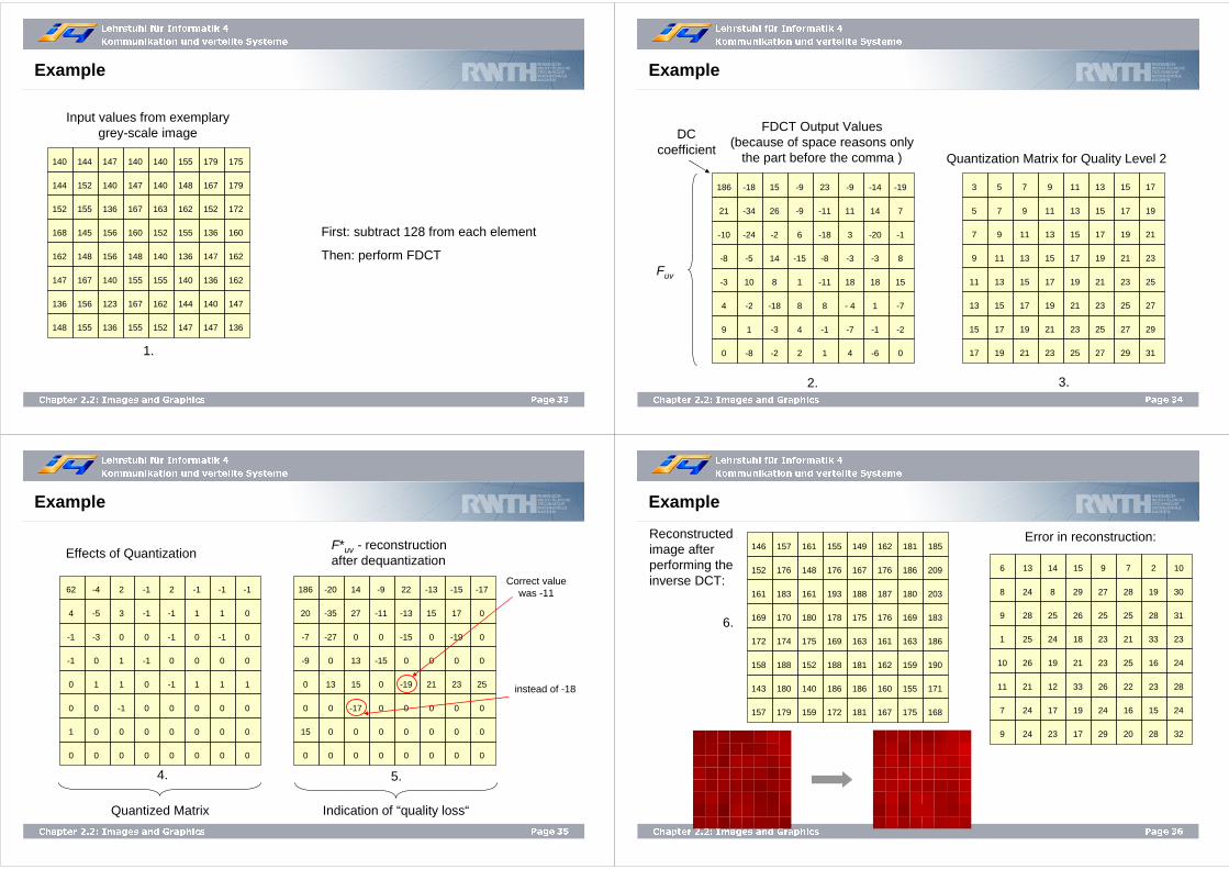
Example

152

144

140

168

162

148

136

147

155

152

144

145

148

155

156

167

136

140

147

156

156

136

123

140

167

147

140

160

148

155

167

155

163

140

140

152

140

152

162

155

162

148

155

155

136

147

144

140

152

167

179

136

147

147

140

136

172

179

175

160

162

136

147

162

Input values from exemplary grey-scale image

1.

First: subtract 128 from each element

Then: perform FDCT




Example

Quantization Matrix for Quality Level 2

3.

7

5

3

9

11

17

15

13

9

7

5

11

13

19

17

15

11

9

7

13

15

21

19

17

13

11

9

15

17

23

21

19

15

13

11

17

19

25

23

21

17

15

13

19

21

27

25

23

19

17

15

21

23

29

27

25

21

19

17

23

25

31

29

27

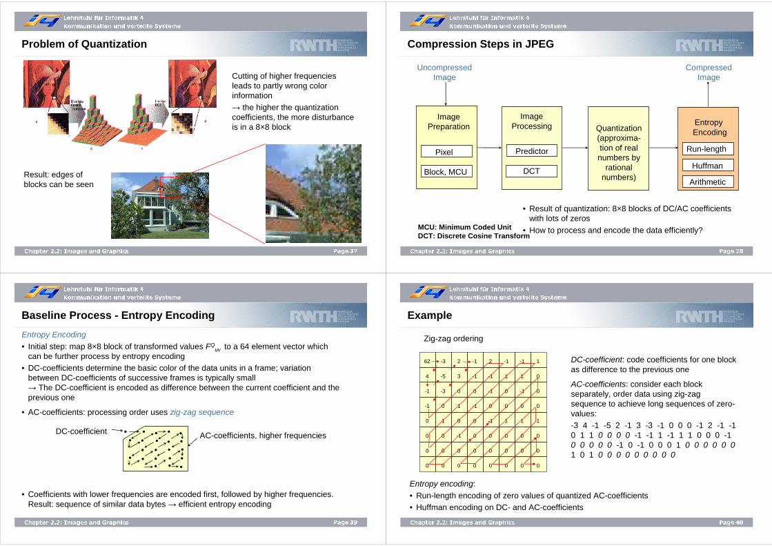
2.

Fuv

DCcoefficient

FDCT Output Values(because of space reasons only

the part before the comma )

-10

21

186

-8

-3

0

9

4

-24

-34

-18

-5

10

-8

1

-2

-2

26

15

14

8

-2

-3

-18

6

-9

-9

-15

1

2

4

8

-18

-11

23

-8

-11

1

-1

8

3

11

-9

-3

18

4

-7

- 4

-20

14

-14

-3

18

-6

-1

1

-1

7

-19

8

15

0

-2

-7




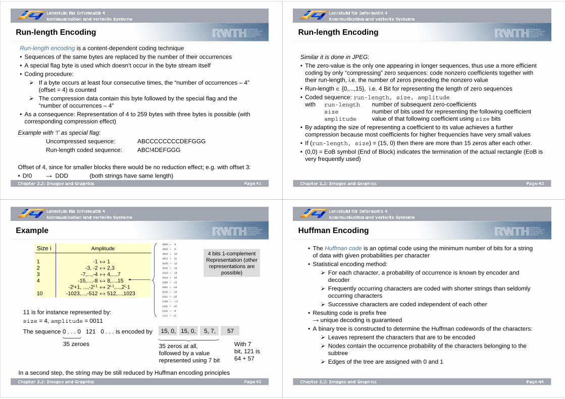
Example

-1

4

62

-1

0

0

1

0

-3

-5

-4

0

1

0

0

0

0

3

2

1

1

0

0

-1

0

-1

-1

-1

0

0

0

0

-1

-1

2

0

-1

0

0

0

0

1

-1

0

1

0

0

0

-1

1

-1

0

1

0

0

0

0

0

-1

0

1

0

0

0

Effects of Quantization

4.

Quantized Matrix

instead of -18

Indication of “quality loss“

-7

20

186

-9

0

0

15

0

-27

-35

-20

0

13

0

0

0

0

27

14

13

15

0

0

-17

0

-11

-9

-15

0

0

0

0

-15

-13

22

0

-19

0

0

0

0

15

-13

0

21

0

0

0

-19

17

-15

0

23

0

0

0

0

0

-17

0

25

0

0

0

Correct valuewas -11

5.

F*uv - reconstructionafter dequantization




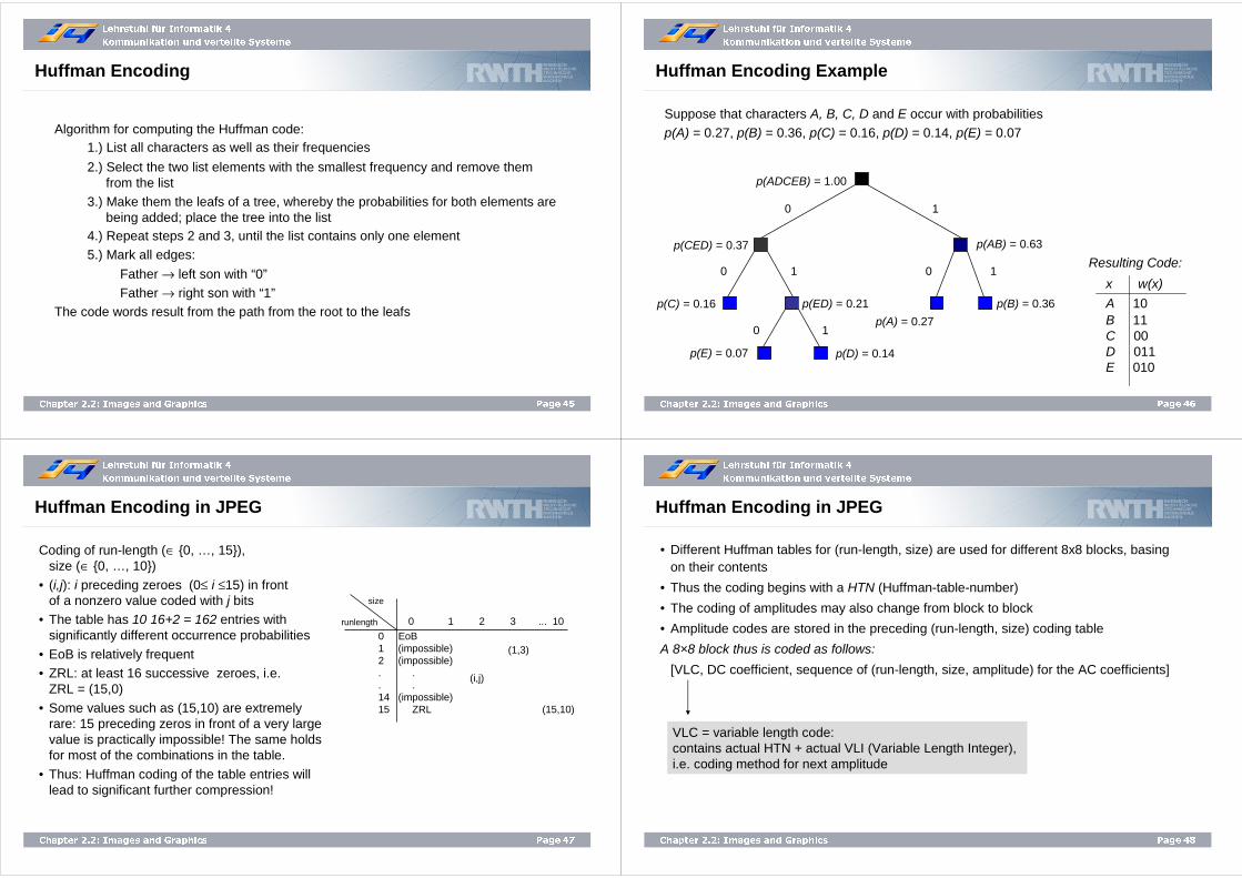
Example

161

152

146

169

172

157

143

158

183

176

157

170

174

179

180

188

161

148

161

180

175

159

140

152

193

176

155

178

169

172

186

188

188

167

149

175

163

181

186

181

187

176

162

176

161

167

160

162

180

186

181

169

163

175

155

159

203

209

185

183

186

168

171

190

Reconstructed image after performing the inverse DCT:

6.9

8

6

1

10

9

7

11

28

24

13

25

26

24

24

21

25

8

14

24

19

23

17

12

26

29

15

18

21

17

19

33

25

27

9

23

23

29

24

26

25

28

7

21

25

20

16

22

28

19

2

33

16

28

15

23

31

30

10

23

24

32

24

28

Error in reconstruction:




Problem of Quantization

Cutting of higher frequencies leads to partly wrong color information

→ the higher the quantization coefficients, the more disturbance is in a 8×8 block

Result: edges of blocks can be seen





ImagePreparation

Pixel


rational numbers)

Block, MCU

Image Processing

Predictor

Entropy Encoding

Run-length

Huffman

Arithmetic

UncompressedImage

CompressedImage

• Result of quantization: 8×8 blocks of DC/AC coefficients with lots of zeros

• How to process and encode the data efficiently?

DCT





Entropy Encoding

• Initial step: map 8×8 block of transformed values FQuv to a 64 element vector which

can be further process by entropy encoding• DC-coefficients determine the basic color of the data units in a frame; variation

between DC-coefficients of successive frames is typically small→ The DC-coefficient is encoded as difference between the current coefficient and the previous one

• AC-coefficients: processing order uses zig-zag sequence

Baseline Process - Entropy Encoding

DC-coefficient AC-coefficients, higher frequencies

•

•• ••••

••

••

••

••

•••

•

•••

• Coefficients with lower frequencies are encoded first, followed by higher frequencies. Result: sequence of similar data bytes → efficient entropy encoding




Example

-1

4

62

-1

0

0

0

0

-3

-5

-3

0

1

0

0

0

0

3

2

1

0

0

0

-1

0

-1

-1

-1

0

0

0

0

-1

-1

2

0

-1

0

0

0

0

1

-1

0

1

0

0

0

-1

1

-1

0

1

0

0

0

0

0

1

0

1

0

0

0

Zig-zag ordering

DC-coefficient: code coefficients for one block as difference to the previous one

AC-coefficients: consider each block separately, order data using zig-zagsequence to achieve long sequences of zero-values:-3 4 -1 -5 2 -1 3 -3 -1 0 0 0 -1 2 -1 -10 1 1 0 0 0 0 -1 -1 1 -1 1 1 0 0 0 -1 0 0 0 0 0 -1 0 -1 0 0 0 1 0 0 0 0 0 01 0 1 0 0 0 0 0 0 0 0 0

Entropy encoding:

• Run-length encoding of zero values of quantized AC-coefficients• Huffman encoding on DC- and AC-coefficients




Run-length Encoding

Run-length encoding is a content-dependent coding technique

• Sequences of the same bytes are replaced by the number of their occurrences• A special flag byte is used which doesn‘t occur in the byte stream itself• Coding procedure:

� If a byte occurs at least four consecutive times, the “number of occurrences – 4”(offset = 4) is counted

� The compression data contain this byte followed by the special flag and the “number of occurrences – 4”

• As a consequence: Representation of 4 to 259 bytes with three bytes is possible (with corresponding compression effect)

Example with ‘!’ as special flag:Uncompressed sequence: ABCCCCCCCCDEFGGG

Run-length coded sequence: ABC!4DEFGGG

Offset of 4, since for smaller blocks there would be no reduction effect; e.g. with offset 3:• D!0 → DDD (both strings have same length)




Run-length Encoding

Similar it is done in JPEG:• The zero-value is the only one appearing in longer sequences, thus use a more efficient

coding by only “compressing” zero sequences: code nonzero coefficients together with their run-length, i.e. the number of zeros preceding the nonzero value

• Run-length ∈ {0,...,15}, i.e. 4 Bit for representing the length of zero sequences• Coded sequence: run-length, size, amplitude

with run-length number of subsequent zero-coefficientssize number of bits used for representing the following coefficientamplitude value of that following coefficient using size bits

• By adapting the size of representing a coefficient to its value achieves a further compression because most coefficients for higher frequencies have very small values

• If (run-length, size) = (15, 0) then there are more than 15 zeros after each other.

• (0,0) = EoB symbol (End of Block) indicates the termination of the actual rectangle (EoB is very frequently used)




Size i Amplitude

1 -1 ↔ 12 -3, -2 ↔ 2,33 -7,...,-4 ↔ 4,...,74 -15,...,-8 ↔ 8,...,15

-2i+1, ...,-2i-1 ↔ 2i-1,...,2i-110 -1023,...,-512 ↔ 512,...,1023

Example

35 zeroes

15, 0, 15, 0, 5, 7, 57

4 bits 1-complementRepresentation (other representations are

possible)

11 is for instance represented by:

size = 4, amplitude = 0011

The sequence 0 . . . 0 121 0 . . . is encoded by

In a second step, the string may be still reduced by Huffman encoding principles

0000 8

0001 9

0010 10

0011 11

0100 12

0101 13

0110 14

0111 15

1000 15

1001 14

1010 13

1011 12

1100 11

1101 10

1110 9

1111

∧

∧

∧

∧

∧

∧

∧

∧

∧

∧

∧

∧

∧

∧

∧

=

=

=

=

=

=

=

=

= −

= −

= −

= −

= −

= −

= −

8∧= −

35 zeros at all, followed by a value represented using 7 bit

With 7 bit, 121 is 64 + 57




Huffman Encoding

• The Huffman code is an optimal code using the minimum number of bits for a string of data with given probabilities per character

• Statistical encoding method: � For each character, a probability of occurrence is known by encoder and

decoder� Frequently occurring characters are coded with shorter strings than seldomly

occurring characters

� Successive characters are coded independent of each other• Resulting code is prefix free → unique decoding is guaranteed

• A binary tree is constructed to determine the Huffman codewords of the characters:� Leaves represent the characters that are to be encoded� Nodes contain the occurrence probability of the characters belonging to the

subtree� Edges of the tree are assigned with 0 and 1




Huffman Encoding

Algorithm for computing the Huffman code:1.) List all characters as well as their frequencies

2.) Select the two list elements with the smallest frequency and remove them from the list

3.) Make them the leafs of a tree, whereby the probabilities for both elements are being added; place the tree into the list

4.) Repeat steps 2 and 3, until the list contains only one element5.) Mark all edges:

Father → left son with “0”Father → right son with “1”

The code words result from the path from the root to the leafs




Huffman Encoding Example

Resulting Code:

p(ADCEB) = 1.00

p(C) = 0.16

0

00

0

1

11

1

p(CED) = 0.37

p(ED) = 0.21

p(E) = 0.07 p(D) = 0.14

p(AB) = 0.63

p(A) = 0.27

p(B) = 0.36

Suppose that characters A, B, C, D and E occur with probabilitiesp(A) = 0.27, p(B) = 0.36, p(C) = 0.16, p(D) = 0.14, p(E) = 0.07

x w(x)

A 10B 11C 00D 011E 010




Huffman Encoding in JPEG

Coding of run-length (∈ {0, …, 15}), size (∈ {0, …, 10})

• (i,j): i preceding zeroes (0≤ i ≤15) in front of a nonzero value coded with j bits

• The table has 10·16+2 = 162 entries with significantly different occurrence probabilities

• EoB is relatively frequent• ZRL: at least 16 successive zeroes, i.e.

ZRL = (15,0)

• Some values such as (15,10) are extremely rare: 15 preceding zeros in front of a very large value is practically impossible! The same holds for most of the combinations in the table.

• Thus: Huffman coding of the table entries will lead to significant further compression!

runlength

0 EoB1 (impossible)2 (impossible). .. .14 (impossible) 15 ZRL

0 1 2 3 ... 10

size

(i,j)

(1,3)

(15,10)




Huffman Encoding in JPEG

• Different Huffman tables for (run-length, size) are used for different 8x8 blocks, basing on their contents

• Thus the coding begins with a HTN (Huffman-table-number)

• The coding of amplitudes may also change from block to block

• Amplitude codes are stored in the preceding (run-length, size) coding table

A 8×8 block thus is coded as follows:

[VLC, DC coefficient, sequence of (run-length, size, amplitude) for the AC coefficients]

VLC = variable length code: contains actual HTN + actual VLI (Variable Length Integer), i.e. coding method for next amplitude




Characteristics:

• Achieves optimality (coding rate) as the Huffman coding

• Difference to Huffman: the entire data stream has an assigned probability, which consists of the probabilities of the contained characters. Coding a character takes place with consideration of all previous characters.

• The data are coded as an interval of real numbers between 0 and 1. Each value within the interval can be used as code word.

• The minimum length of the code is determined by the assigned probability.

• Disadvantage: the data stream can be decoded only as a whole.

Alternative to Huffman: Arithmetic Coding




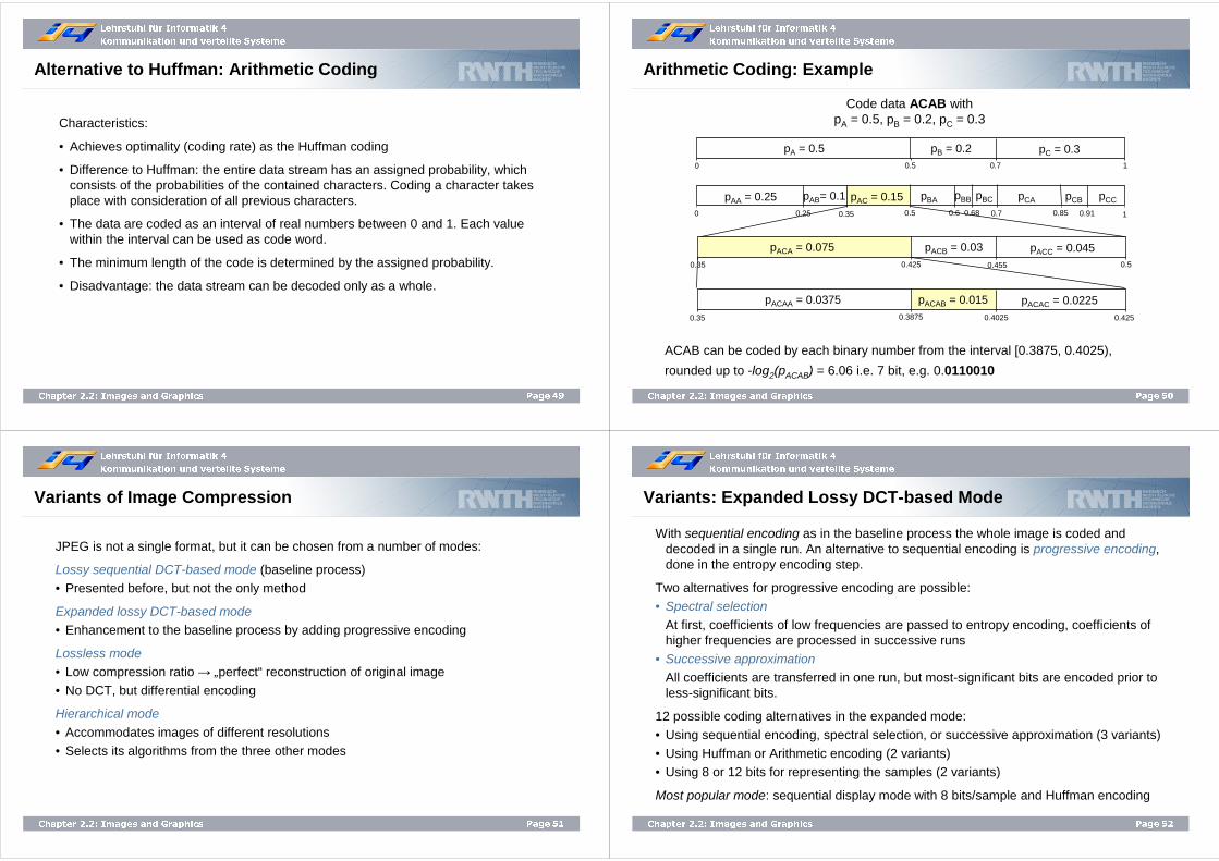
Code data ACAB with pA = 0.5, pB = 0.2, pC = 0.3

pA = 0.5 pC = 0.3

ACAB can be coded by each binary number from the interval [0.3875, 0.4025),

rounded up to -log2(pACAB) = 6.06 i.e. 7 bit, e.g. 0.0110010

pB = 0.2

pAA = 0.25 pAC = 0.15pAB= 0.1 pBA pBCpBB pCA pCB pCC

pACA = 0.075 pACC = 0.045pACB = 0.03

pACAA = 0.0375 pACAC = 0.0225pACAB = 0.015

0

0

0.35

0.35

0.5

0.25 0.35 0.5

0.425

0.425

0.7 1

10.70.6 0.68 0.85 0.91

0.50.455

0.3875 0.4025

Arithmetic Coding: Example




Variants of Image Compression

JPEG is not a single format, but it can be chosen from a number of modes:

Lossy sequential DCT-based mode (baseline process)• Presented before, but not the only method

Expanded lossy DCT-based mode• Enhancement to the baseline process by adding progressive encoding

Lossless mode• Low compression ratio → „perfect“ reconstruction of original image

• No DCT, but differential encoding

Hierarchical mode

• Accommodates images of different resolutions• Selects its algorithms from the three other modes




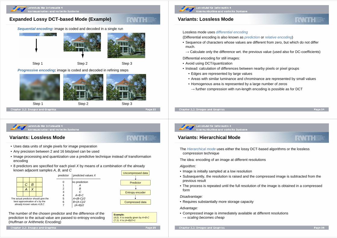
With sequential encoding as in the baseline process the whole image is coded and decoded in a single run. An alternative to sequential encoding is progressive encoding, done in the entropy encoding step.

Two alternatives for progressive encoding are possible:

• Spectral selectionAt first, coefficients of low frequencies are passed to entropy encoding, coefficients of higher frequencies are processed in successive runs

• Successive approximationAll coefficients are transferred in one run, but most-significant bits are encoded prior to less-significant bits.

12 possible coding alternatives in the expanded mode:• Using sequential encoding, spectral selection, or successive approximation (3 variants)

• Using Huffman or Arithmetic encoding (2 variants)• Using 8 or 12 bits for representing the samples (2 variants)

Most popular mode: sequential display mode with 8 bits/sample and Huffman encoding

Variants: Expanded Lossy DCT-based Mode




Expanded Lossy DCT-based Mode (Example)

Progressive encoding: image is coded and decoded in refining steps

Sequential encoding: image is coded and decoded in a single run

Step 1 Step 2 Step 3

Step 1 Step 2 Step 3




Variants: Lossless Mode

Lossless mode uses differential encoding(Differential encoding is also known as prediction or relative encoding)• Sequence of characters whose values are different from zero, but which do not differ

much.→ Calculate only the difference wrt. the previous value (used also for DC-coefficients)

Differential encoding for still images:• Avoid using DCT/quantization• Instead: calculation of differences between nearby pixels or pixel groups

• Edges are represented by large values• Areas with similar luminance and chrominance are represented by small values

• Homogenous area is represented by a large number of zeros → further compression with run-length encoding is possible as for DCT




Variants: Lossless Mode

• Uses data units of single pixels for image preparation

• Any precision between 2 and 16 bits/pixel can be used• Image processing and quantization use a predictive technique instead of transformation

encoding

• 8 predictors are specified for each pixel X by means of a combination of the already known adjacent samples A, B, and C

predictor predicted values X

0 no prediction1 A2 B3 C4 A+B-C5 A+(B-C)/26 B+(A-C)/27 (A+B)/2

The number of the chosen predictor and the difference of the prediction to the actual value are passed to entropy encoding (Huffman or Arithmetic Encoding)

Example:(4,0): X is exactly given by A+B-C(7,1): X is (A+B)/2+1

ABCX

The actual predictor should give thebest approximation of x by the already known values A,B,C

Uncompressed data

Predictor

Entropy encoder

Compressed data




Variants: Hierarchical Mode

The Hierarchical mode uses either the lossy DCT-based algorithms or the lossless compression technique

The idea: encoding of an image at different resolutions

Algorithm:• Image is initially sampled at a low resolution• Subsequently, the resolution is raised and the compressed image is subtracted from the

previous result• The process is repeated until the full resolution of the image is obtained in a compressed

form

Disadvantage:• Requires substantially more storage capacity

Advantage:• Compressed image is immediately available at different resolutions→ scaling becomes cheap

Digital Image Representation - nets.rwth-aachen.de · • Digital image representation ... Chapter...

Documents

Transcript of Digital Image Representation - nets.rwth-aachen.de · • Digital image representation ... Chapter...