No.05-E-12 September 2005

Changes in the Demand for Skilled Labor within Japan’s Manufacturing Sector: Effects of Skill-Biased Technological Change and Globalization Hitoshi Sasaki* hitoshi.sasaki@boj.or.jp Kenichi Sakura** kenichi.sakura@boj.or.jp Bank of Japan 2-1-1 Nihonbashi Hongoku-cho, Chuo-ku, Tokyo 103-8660

* Research and Statistics Department ** Research and Statistics Department Papers in the Bank of Japan Working Paper Series are circulated in order to stimulate discussion and comments. Views expressed are those of authors and do not necessarily reflect those of the Bank. If you have any comment or question on the working paper series, please contact each author. When making a copy or reproduction of the content for commercial purposes, please contact the Public Relations Department (webmaster@info.boj.or.jp) at the Bank in advance to request permission. When making a copy or reproduction, the source, Bank of Japan Working Paper Series, should explicitly be credited.

Bank of Japan Working Paper Series

1

CHANGES IN THE DEMAND FOR SKILLED LABOR

WITHIN JAPAN’S MANUFACTURING SECTOR: EFFECTS OF SKILL-BIASED TECHNOLOGICAL CHANGE AND

GLOBALIZATION*

Hitoshi Sasaki†

Research and Statistics Department, Bank of Japan.

and Kenichi Sakura‡

Research and Statistics Department, Bank of Japan.

September, 2005

Abstract

This paper examines the demand shift toward workers who are university graduates in terms of skill-biased technological change (SBTC) and globalization, both of which utilize relatively more workers with specific skills. According to the results of our empirical study, which used the major groups of Japan’s manufacturing panel data from the 1988-2003, it is clear that the increase in the relative demand for university graduates is closely related to the R&D expenditures ratio (SBTC) and the import ratio from the East Asian countries or the foreign production ratio (globalization). This suggests that there has been a demand shift toward highly educated workers in Japan’s manufacturing sector due to both SBTC and globalization.

Keywords: skilled workers; skill-biased technological change; globalization JEL Classification Number: F16; J23; O30

* We are especially grateful to Izumi Takagawa for her capable assistance. We also thank Kyoji Fukao, Kojiro Sakurai, Eiichi Tomiura, Masahiro Higo, Takeshi Kimura, seminar participants at the Japan Economic Association 2005 Spring meetings, and other officials of the Bank of Japan for their helpful comments and suggestions. Of course, we are solely responsible for any remaining errors in this paper. The views presented in this paper are those of the authors, and not those of the Bank of Japan. † E-mail: hitoshi.sasaki@boj.or.jp ‡ E-mail: kenichi.sakura@boj.or.jp

2

1. INTRODUCTION

In many advanced countries, including the United States, the wage inequality between skilled and unskilled workers has increased from the 1980s to 1990s.1 It has been pointed out that the inequality is caused by the demand shift from unskilled to skilled workers. This paper is motivated by our inference that the demand shift toward skilled workers has also been in progress recently in Japan.

One main factor that caused the demand shift toward skilled workers is skill-biased technological change (SBTC, hereafter). SBTC is one particular type of technological change that utilizes relatively more workers with specific skills. It includes skills such as, for example, “IT-related technique,” which is necessary to use computers and software, “installation of manufacturing equipments,” which requires advanced techniques and skills, and “research and development” (R&D, hereafter).

Another important factor is the effects of globalization, especially the increase in trade with developing countries. They correspond to the expanding imports of cheap and unskilled-labor-intensive products due to the increase in trade with developing countries, and to foreign outsourcing of a part of domestic manufacturing processes—which require relatively less-skilled domestic labor—to those countries, where firms develop global production activities.

This paper examines the effects of both SBTC and globalization on the demand shift toward skilled labor in Japan’s manufacturing. Before performing a concrete analysis in the next section, we first review several previous studies from the United States and Japan.

Many studies have been carried out in the United States, since the wage inequality there between skilled and unskilled workers has recently grown, as we noted above. Especially, the evaluation of the effects of SBTC and globalization on the demand shift toward skilled workers has been a great concern, because SBTC is closely associated with educational and/or technological policies, while globalization has much to do with trade policy. These previous studies have reported that both SBTC (such as computer investment ratio) and globalization (such as foreign outsourcing to developing countries or trade expansion with those countries) have caused the demand shift from production workers (unskilled workers) to non-production workers (skilled workers). There is no consensus yet, however, on the relative impacts of these two effects, which depend on the specifications of the estimated models and on the

1 The rise in wage inequality is clearly observed, especially in the United States and the United

Kingdom, in several industrialized countries according to Freeman and Katz (1994). These differences in wage inequalities across developed countries arise from the differences in labor demand and supply factors and some institutional aspects concerning wage-setting such as unionization, minimum wage systems, and favorable treatments for unskilled labor such as unemployment insurance.

3

variables in use.2 In contrast, there have been only a few related studies in Japan, partly because

wage inequality has not been an open question thus far. Among the important studies in recent years, Sakurai (2001) has found that recent technological changes such as IT are key in causing the demand shift from production workers to non-production workers.3 As related to the effects of globalization, Sakurai (2000) has reported that the relationship between the progress of foreign outsourcing and the demand shift toward non-production workers seems to be unclear. Meanwhile, Head and Ries (2000) have pointed out that increased employment in the overseas affiliates has worked as a key factor for the demand shift toward non-production workers. The above-mentioned studies have analyzed the periods of the 1980s and/or the beginning of the 1990s, and have likewise investigated the effects of SBTC and globalization on the demand shift toward skilled workers, separately. In this respect, Ito and Fukao (2004) have extended the data to 2000, and have also analyzed the demand shift toward skilled workers, taking into account both SBTC and globalization simultaneously. They have reported that the effects of SBTC, such as IT and R&D, on the demand shift are significant, while those of globalization—including the “vertical intra-industry trade ratio” and the “foreign outsourcing ratio” with the East Asian countries—vary, depending on the definition of “skilled labor” or on the variables employed in the empirical study.

On the basis of these previous studies, this paper has two main features: first, we have examined the periods from the 1990s to early 2000s, when the effects of SBTC and globalization are likely to have mostly pervaded in Japan; and second, we have tried to evaluate the relative impacts of both SBTC and globalization on the demand shift toward skilled workers, taking account of them simultaneously. These two points have not yet been sufficiently examined by the previous Japanese studies.

This study covers the manufacturing sector only; it excludes the non-manufacturing sector to examine the relationship between the effects of globalization and the demand shift toward skilled workers. Moreover, it focuses on regular employment, since the ratio of irregular employment to total employment is still low in Japan’s manufacturing. 4 Finally, we assume that worker skills are classified by their educational levels; therefore, we regard the university graduates as

2 For example, Berman et al. (1994) and Autor et al. (1998) have reported that SBTC has greatly contributed to the demand shift toward skilled labor while the effects of globalization have been trivial. On the other hand, Sachs and Shatz (1994), Wood (1994), Bernard and Jensen (1997) and Feenstra and Hanson (1996a, 1996b, 1999) have reported that globalization too, along with SBTC, has been a key factor.

3 Sakurai (2004) has developed the analysis of Sakurai (2001), reporting that recent technological change had been an important factor in the demand shift toward highly educated workers.

4 The percentage of part-time workers in the “manufacturing” industry is only about 10 percent according to the “Monthly Labor Survey 2003” of the Ministry of Health, Labor and Welfare.

4

“skilled,” and the other workers (non-university graduate workers) as “unskilled.”5 The remainder of this paper is organized as follows. In Section 2, we describe the

process of the share in the wage bill of skilled workers (proportion of the wage bill paid for skilled workers to the total wage bill) rising when the relative demand for skilled workers increases, due to the effects of SBTC and/or globalization. In Section 3, we examine whether the relative demand for university graduates, defined as “skilled” workers in this study, have recently increased in Japan by using the wage data compiled in the “Basic Survey on Wage Structure” (BSWS, hereafter) by the Ministry of Health, Labor and Welfare. In Section 4, we perform an empirical analysis to investigate whether both SBTC and globalization have increased the relative demand for university graduates with the use of panel data by industry of Japan’s manufacturing sector from 1988-2003. Section 5 concludes.

2. THE DEMAND SHIFT FROM UNSKILLED TO SKILLED WORKERS

This section describes the process in which the share in wage bill of skilled workers increases when the demand shift from unskilled to skilled workers occurs within each industry due to SBTC and/or globalization.

An industry i is assumed to produce its output using both skilled H and unskilled labor L as input factors whose unit prices (i.e., wages) are described as

Hw and Lw , respectively. Taking skilled labor on the vertical axis and unskilled labor on the horizontal axis, the isoquant curve of industry i should be shown as 00 yy in Figure 1(1). When the economy is in equilibrium at point A under perfect competition, the relative wage and the relative labor ratio are described as HL ww / and

LH / , respectively. When a technological change takes place, the isoquant curve inwardly shifts to

the origin; the industry i is now capable of producing a given amount of output with less inputs. If this technological change is skill-biased (SBTC), the isoquant curve shifts inward so as to save the unskilled labor relative to the skilled one. This shift is expressed as an inward shift from 00 yy to 11 yy in Figure 1(2). After the

5 We can apply a production/non-production classification instead of an educational classification; we

can regard production/non-production workers as unskilled/skilled workers. However, the production/non-production classification in the major groups of manufacturing in the standard industrial classification is not available in the BSWS; it is only available in the division in the standard industrial classification (the production/non-production classification in the major groups of manufacturing is available in the “Census of Manufactures” by the Ministry of Economy, Trade and Industry only before 1990). According to the “Basic Survey on Wage Structure 2003CY” by the Ministry of Health, Labor and Welfare, the proportion of university graduates in production workers is less than 10 percent in the manufacturing as a whole, while the proportion in non-production workers is more than 50 percent. Therefore, it would not become an issue to classify both the highly educated and non-production workers as skilled.

5

adjustments of labor inputs and wages,6 the economy will finally reach equilibrium at point B . Comparing the relative labor ratios and relative wage ratios at both economies A and B , the relative labor ratio increases ( LHLH ′′< // ) while the relative wage ratio declines ( HLHL wwww ′′> // ). Consequently, the share in the wage bill of skilled workers at economy B (the right side of the inequality below) exceeds that at economy A (the left-hand side of the inequality below):7

44 344 2144 344 21BEconomyatworkersskilledofsharebillwage

HL

H

AEconomyatworkersskilledofsharebillwage

HL

H

HwLwHw

HwLwHw

)()( ′′+′′′′

<+

The above analysis has demonstrated that the share in the wage bill of skilled

workers rises as a result of the increase in relative demand for skilled workers within a same industry. Such a demand shift toward skilled workers within an industry occurs not only by SBTC but also by globalization, particularly, by foreign outsourcing activities to developing countries where unskilled workers are abundant; firms become multinational and transfer a part of production processes, which use relatively more unskilled labor, to developing countries; then, they change the sources of procurement of intermediate and final goods from domestic supplies that used to be provided domestically, to imports from those countries, resulting in the increase (decrease) in the relative demand for skilled (unskilled) labor within each industry.8

Finally, it is worth mentioning that the foreign outsourcing effects stated above and the standard effects of changes in relative prices of tradable goods, i.e., the price effects of “Stolper-Samuelson theorem,” are the same in that the trade expansion with developing countries increases the relative demand for skilled labor; although the ways of the demand shift toward skilled labor are different in both cases. The demand shift takes place toward skilled labor within an industry in the former, while it does so between industries in the latter where the shift arises from the industries with relatively abundant unskilled labor to those with relatively abundant skilled ones. Therefore, the demand shift to skilled labor by globalization takes place both within and between industries.

6 Here, the number of skilled and unskilled workers is exogenously given, since we focus on the

change in the labor demand. Thus, the labor input with an increase in the relative demand for skilled labor is adjusted by working hours, not by number of workers.

7 When the Hicks-neutral technological change occurs, the isoquant curve shifts inward, which nevertheless affect neither the relative labor ratio nor the relative wage ratio. Consequently, the share in the wage bill of skilled workers remains unchanged after the technological change.

8 Concerning foreign outsourcing effects, strictly speaking, we need to incorporate in the model the transactions of parts and final goods in each production stage between industrialized and developing countries, rather than discussing on the basis of producing unique good, as shown in Figure 1. For example, Feenstra and Hanson (1996a) have developed a theoretical model that describes the process in which foreign outsourcing raises the relative demand for skilled labor within the same industry.

6

Taking into account the above analytical framework, the analysis of this paper focuses on the effects of SBTC and globalization on the demand shift from unskilled (non-university graduate workers) to skilled workers (university graduate workers).

3. AN INCREASE IN THE DEMAND FOR HIGHLY EDUCATED WORKERS IN JAPAN’S MANUFACTURING SECTOR

We examine whether the relative demand for highly-educated workers has recently increased in Japan before analyzing the relationship between SBTC and/or globalization and the demand shift toward workers with college degrees. We use the wage data of regular male workers of Japan’s manufacturing from the BSWS.

Section 3.1 measures and examines the hourly wage differentials between university graduates and workers without a college education since 1985 by estimating the “Mincer-type” wage function, taking into account worker characteristics, such as their working years. In Section 3.2, we decompose the changes in the wage bill share of university graduate workers into the “within” and the “between” shift to obtain implications in terms of the effects of SBTC and globalization.

3.1 Measuring the Hourly Wage Differentials Between Workers With and Without University Degrees

According to the human capital theory, education is assumed to work for accumulating the human capital of workers as its investment effect, consequently augmenting their wages. The education includes both schooling and job training through business. The “Mincer-type” wage function is derived on the basis of this human capital theory (Mincer, 1974). In this framework, the logarithm of worker’s hourly wage is described as a function of his duration of schooling, working years, and its square:

221ln KKtw γγβα +++= (3-1)

where wln represents the logarithm of worker’s hourly wage; t denotes years of schooling; K is his working years; α is a constant term; and β , 1γ and 2γ are parameters, respectively.

In this section, we estimate the following equation (3-2) for 1985, 1990, 1995, 2000, and 2003, based on (3-1), with the wage sample of regular male workers of 17 manufacturing industries9 in the BSWS. The estimation is performed by weighting

9 The 17 industries include “Food, Beverages and Tobacco,” “Textile Mill Products,” “Apparel and Other Finished Products,” “Lumber and Wood Products,” “Furniture and Fixtures,” “Pulp, Paper and Paper Products,” “Printing and Allied Industries,” “Chemical and Allied Products,” “Rubber Products,”

7

each wage sample by its number of workers (weighted least squares), dealing with a possible heteroscedasticity in the error term:10

∑ =+=

2

1)()(ln

gg

igi kinbawage

ikFkikj

Ejijh

Dhih uDfDeDd ++++ ∑∑∑ ===

16

1

2

1

3

1 (3-2)

where i denotes the subscript of the wage sample; )(ln iwage is the logarithm of scheduled hourly wage, which is equivalent to the ratio of the scheduled cash earnings (thousands of yen per month) to scheduled actual hours worked (hours per month);

)( ikin is the length of service (years); DhiD , Ej

iD and FkiD represent the school

career, the size of enterprise and the industry dummies, respectively; a represents a constant term; gb , hd , je and kf are parameters; and iu denotes the error term.

Three kinds of dummy variables are defined as follows:

School career dummies: DhiD

1DiD … university graduate dummy (university graduate workers 1, others 0);

2DiD … higher professional school and junior college graduate dummy (higher

professional school or junior college graduate workers 1, others 0); 3D

iD … high school graduate dummy (senior high school graduate workers 1, others 0).

Size of enterprise dummies: EjiD

1EiD … large enterprise dummy (enterprises with 1,000 or more employees 1, others 0);

2EiD … medium enterprise dummy (enterprises with 100-999 employees 1, others 0).

Industry dummies: Fk

iD Industry dummy variables consist of 16 types of manufacturing industries; the base industry is the “manufacture of food, beverages and tobacco.”

By estimating (3-2), we can quantitatively evaluate the wage differentials among

workers with different educational backgrounds, after controlling worker characteristics contained in the individual wage sample, i .11 The estimation results are shown in Table 1. For example, the wage differential between university graduate

“Ceramic, Stone and Clay Products,” “Iron and Steel,” “Non-Ferrous Metals and Products,” “Fabricated Metal Products,” “General Machinery,” “Electrical Machinery, Equipment and Supplies,” “Transportation Equipment,” and “Precision Instruments and Machinery.”

10 We can obtain 1,836 wage samples at most: that is, 17 (number of industries) × 9 (number of age classes from 20 to 65 years old) × 4 (number of educational background classes) × 3 (number of firm size classes).

11 As a related study, Sakurai (2004) has evaluated the wage differentials among different educational backgrounds during the 1985-2000 by estimating the “Mincer-type” wage function, which is similar to equation (3-2), indicating their interpretations and problems.

8

workers and high school graduate workers is calculated as the difference between the estimated parameter on the “high school dummy” and that on the “university dummy” (i.e., 31

ˆˆ dd − ).12 Figure 2 describes the chronological changes in the measured hourly wage differentials between university graduate workers and non-university graduate workers from the 1985-2003. These wage differentials have slightly increased during the period, even though it is still necessary to take estimation errors into account.

An increase in the supply of university graduate workers accompanied by the recent “popularization of higher education” would work to lower the hourly wages of university graduate workers, at least relatively. The above estimation results nevertheless suggest that the magnitude of the increase in relative demand for university-educated workers has been large enough to cancel out the downward pressure on hourly wages due to such a supply factor.

3.2 Decomposition of the Increase in the Wage Bill Share of University Graduates into “Within” and “Between” Shifts

We now focus on the changes in the wage bill share of university graduates since 1985. Typically, the wage bill data—from which the effects of various worker characteristics should be eliminated, following the analysis conducted in the Section 3.1—is used. However, for simplicity, we calculate the wage bill as the “average scheduled cash earnings” times the “number of male workers.”

First, according to the chronological change in the wage bill share of university graduates in overall manufacturing in Table 2(1), the wage bill share has consistently increased since 1985, and in particular the rate of increase has somewhat accelerated since 2000. The average rate of annual change from the 1985-2003 is +0.60 percentage points, which is comparable to that in the U.S. manufacturing sector from 1980-1996, i.e., +0.74 percentage points.13 Furthermore, the wage bill share has increased in all industries, except for a part of periods, as shown in Table 2(2). As the backgrounds of these movements, it should be pointed out that there exists an increase in the relative demand for university graduate workers by industry, taking account of the results obtained from the analysis in 3.1, in addition to the increase in the number of

12 A few points should be noted regarding the estimation results except for the school career dummies in Table 1. First, the parameter estimate on working years, 1̂b , is positive, while that on its square, 2b̂ , is negative; this suggests that the scheduled hourly wages of workers increase with the working years, although the rate of increase lowers with the years. In addition, among the size of enterprise dummies, the parameter on large enterprise dummy is estimated to be positive; this indicates that the scheduled hourly wages of workers belonging to large enterprises are higher than those of workers belonging to both medium and small enterprises. Finally, the parameters on industry dummies mean the industrial premiums on the basis of the “Beverages, Tobacco and Food” industry.

13 According to Autor et al. (1998), the rate of change in the wage bill share of university graduates in U.S. manufacturing is 0.908 percentage points during the 1980-1990 period, while that during the 1990-1996 period is 0.452 percentage points.

9

university graduates, coupled with the “popularization of higher education.” Let us now consider the backgrounds of the increase in the wage bill share of

university graduates; the increase in the wage bill share of university graduates is decomposed into the “between” and the “within” shifts; the former is approached by the shift of university graduate workers across industries while the latter is by the increase of university graduates within each industry.14 To be more precise, the decomposition is shown in the following equation (3-3): i.e., the “between” shift represents the increase in the wage bill of industries where the wage bill shares of university-educated workers are high, whereas the “within” shift represents the increase in the wage bill share of university graduates within the same industry:

4342143421shiftwithin

n

ii

Hi

shiftbetween

n

i

Hii

H pssps ∑∑==

∆+∆=∆11

(3-3)

i = 1, … , n : industries included in the major groups of manufacturing (n = 17);

WWs HH /= : wage bill share of university graduates in all manufacturing; His = i

Hi WW / : wage bill share of university graduates in industry i ;

ip = WWi / : wage bill share of industry i ’s workers in all manufacturing. where ∆ represents the changes in variables in percentage points; is the average of two periods; W is the wage bill of all manufacturing; HW is the wage bill of university graduates in all manufacturing; iW is the wage bill of industry i ; H

iW is the wage bill of university graduate workers of industry i .

The “between” shift expressed as a first term in the right side of (3-3) is led to by the change in industry structure accompanied by the changes in either domestic and international demands for products or sector productivity shocks. Meanwhile, the “within” shift expressed as the second term is approached by the increase in the relative demand for university graduates within the same industries accompanied by the effects of SBTC and/or those of globalization. If our hypothesis—that either SBTC or globalization serves to increase the relative demand for university graduate workers—is true, the change in the wage bill share of university graduate workers should be brought about by the effects of the “within” shift rather than by those of the “between” shift.

Table 3(1) shows the results of the decomposition into the “between” and the “within” shifts of the wage bill share of university graduates in Japan’s manufacturing sector according to (3-3). It shows that the contribution rate of the “within” shift (approximately 90 percent) largely exceeds that of the “between” shift (approximately

14 This procedure is based on the analysis of Berman et al. (1994).

10

10 percent) in any period after 1985. Table 3(2) shows the results of further decomposition of the “within” and

“between” shifts of the wage bill share of university graduates in Japan’s manufacturing sector during the period into the parts of contributions by industry. As for the “within” shift, the wage bill shares of university graduates have increased in all industries. Above all, the rises are prominent in the industries such as “general machinery,” “electrical machinery,” “transportation equipment,” and “precision machinery.” Subsequently, as for the “between” shift, the wage bill shares of university graduates have declined in many industries, including “textiles,” “apparel,” “lumber and wood,” “furniture and fixtures,” “ceramics, stones and clay,” “iron and steel,” “nonferrous metals,” and “fabricated metals,” all of which are the “import competing industries” under the pressure of recently intensified international competition. Meanwhile, the wage bill share has increased in industries such as “general machinery,” “electrical machinery,” “transportation equipment” and “precision machinery,” i.e., the exporting industries mentioned above.

Summing up, it can be concluded that the wage bill share of university graduate workers has increased mostly by the effects of the “within” shift, in which the ratio of university graduate workers rises within the same industry, accompanied by the effects of the “between” shift, in which university graduate workers have shifted toward the highly competitive industries from the industries which have lost their international competitiveness. This development is consistent with our hypothesis that the relative demand for university graduate workers within the same industry has increased due to SBTC and the expansion of foreign outsourcing.

4. EMPIRICAL ANALYSIS

The analyses up to the previous sections have made it clear that, in Japan, the demand for university-educated workers has increased as compared to the demand for workers without a university degree, and that the increase in the relative demand for university graduates has occurred mainly within the same industry. In this section, we perform an empirical analysis on the effects of SBTC and globalization, both of which are, in general, regarded as the main causes of the demand increases for university graduates, using the panel data by industry of Japan’s manufacturing sector.

4.1 Econometric Model Issues

(1) Derivation of the Cost Share Equation

The cost share equation, on which the following empirical analysis is based, is

11

derived based on the framework adopted in the seminal study of Berman et al. (1994). Let us assume that an industry i within the manufacturing sector produces

output with its input factors of capital, iK , unskilled labor, iL and skilled labor, iH . The capital is assumed to be a fixed factor in the short run while both types of labor are to be variable factors.15 The structural factor, such as SBTC and/or globalization, is denoted as iZ , which shifts the production and cost of industry i . Under these assumptions, we set the following variable cost function, V

iC , as the translog form:

tZYKwC tiZiYiKpp

ipVi αααααα +++++= ∑ lnlnlnlnln 0

)lnlnlnlnln(5.0 2222 ∑ ∑+++++p

qi

piq pqttiZZiYYiKK wwtZYK γαααα

itZiiKZitKiiYZitYiiYK ZtZKKtZYYtKY lnlnlnlnlnlnlnlnln αααααα ++++++

∑∑∑∑ ++++p

pi

tpp

pii

Zpp

pii

Kpp

pii

Yp wtwZwKwY lnlnlnlnlnlnln ρρρρ

(4-1) where p

iw denotes the price of variable factor; t is the time trend effect. The following cost share equation is obtained by differentiating the translog variable cost function (4-1) with respect to the logarithm of the variable factor price, p

iwln , and applying Shepard’s Lemma:

twZKYsC

dwwC t

pqqiqpi

Zpi

Kpi

Ypp

piV

i

pi

pi

pi

Vi ργρρρα +++++===

∂∂ ∑ lnlnlnln

lnln

(4-2) where p

id represents the demand for variable factor with its factor price, piw . The

condition for the translog variable cost function in equation (4-1) to be homogeneous of degree one with respect to the variable factor price, p

iw , is for the following equation (4-3) to hold:16

∑ ∑ ∑∑∑∑ ======p p p

tp

Zp

Kpp

Ypq pqp pq 0ρρρργγ and

15 Here we assume the labor and capital to be, a priori, variable and quasi-fixed, respectively,

irrespective of their types. In this respect, some authors have expressed doubts on whether this assumption actually holds in Japan. Nishimura and Minetaki (2004), for instance, classifies the labor by educational backgrounds (high/low-educated) and age (old/young), and the capital by IT or non-IT, then examining their variability, individually. Consequently, old and poorly educated workers are reported to be a short-term fixed factor, since aged skills are required under “Japan’s long-term employment practice,” and on the shop-floor; IT-related capital, meanwhile, is determined to be short-term variable factor, since software and computers can be replaced in the short run.

16 The symmetry of parameters is also assumed, i.e., qppq γγ = .

12

1=∑p pα (4-3)

In addition, we impose the following restriction of the constant returns to scale on the cost share equation (4-2).

0=+ Kp

Yp ρρ (4-4)

The variable factors in the cost minimization problem here are unskilled and skilled labors, i.e., iL and iH , respectively. Taking account of the restrictions of both equations (4-3) and (4-4), the cost share equation (4-2) can thus be rewritten by regarding the variable factor price, p

iw , included in the translog variable cost function (4-1), as the factor price of skilled labor, H

iw , as follows:

tZYK

ww

s ii

iLi

Hi

iHi δλµγα ++++= ln)(ln)(ln (4-5)

where H

is represents the ratio of the wage bill of skilled workers, i.e., a variable factor, to the total variable cost: i.e., the wage bill share of skilled workers,

)/( iLii

Hii

Hi LwHwHw + . )/(ln L

iHi ww is a logarithm of the relative wage ratio between

skilled and unskilled workers; )/(ln ii YK is the logarithm of capital intensity; iZln is the logarithm of structural variable; iα is the constant term; γ , µ , λ and δ are parameters.

The feature of the cost share equation is that the wage bill share of skilled workers is represented as the linear function of structural and other controlling variables. In Section 2, we have illustrated the process that the increase in the relative demand for skilled workers due to the effects of SBTC and/or foreign outsourcing leads to a rise in the wage bill share of skilled workers. In this respect, we can perform an empirical study to examine the above mechanism by estimating (4-5) with the use of industry-level data under the assumption that the cost functions (4-1) are identical across industries.

One supplementary point should be noted before specifying the estimation model in the following (2, below). The capital intensity and the structural variables of the third and fourth terms included in the right side of (4-5) are both assumed to fluctuate exogenously. However, it is hardly possible to assume that the relative wage, i.e., the second term of (4-5), varies exogenously as long as it represents the relative quality between skilled and unskilled workers. In such a case, we can possibly deal with the problem by estimating the model with the instrumental variables correlated with relative wage. However, since it is in fact difficult to find the appropriate instrumental

13

variables, we then exclude the term from the estimation model after the previous studies, including Berman et al. (1994).

(2) Model Specification

We use the balanced panel data of the major groups of manufacturing (14 industries17) from 1988-2003.18 The estimation model is based on the cost share equation (4-5), which however excludes the relative wage of the second term in the right side of the equation, adding the error term and fourth as follows:

titititiHti Z

YKs εφαλµα +++++= )(ln (4-6)

where i is the subscript of industry included in the major groups of manufacturing; t is the time subscript; H

tis is the wage bill share of university graduate workers; α is the constant term; both µ and λ are parameters assumed to be identical across industries i ; iα is the individual effects by industry; tφ is the time effects; and

tiε is the error term, i.e., the idiosyncratic shock. The structural variable, tiZ , of the third term in the right side of (4-6) includes

the terms that represent the effects of globalization and SBTC. The import ratio from East Asia, tiM , and the foreign production ratio, tiF , are used to denote the effects of globalization.19 Moreover, the IT investment ratio, computer investment ratio, and R&D expenditures ratio are considered to be suited for representing the effects of

17 The 14 industries include “Food, Beverages, and Tobacco,” “Textile Mill Products Including

Apparel and Other Finished Products,” “Pulp, Paper, and Paper Products,” “Printing and Allied Industries,” “Chemical and Allied Products,” “Rubber Products,” “Ceramic, Stone, and Clay Products,” “Iron and Steel,” “Non-Ferrous Metals and Products,” “Fabricated Metal Products,” “General Machinery,” “Electrical Machinery, Equipment and Supplies,” “Transportation Equipment,” and “Precision Instruments and Machinery.”

18 Regarding the previous Japanese studies based on the major groups of manufacturing, the sample number used in those empirical studies is unlikely to be sufficient, since there is a limited number of industries. In this respect, the previously cited Ito and Fukao (2004) has used the data of 35 industries of Japan’s manufacturing sector during the period 1988-2000, which greatly improves the small sample problem on these empirical studies. This paper has also constructed the balanced panel data consisting of 14 industries over 16 years, allowing us to secure, at most, 224 samples.

19 Because the East Asian countries possess relatively more abundant unskilled labor than does Japan, Japan’s multinational companies promote foreign outsourcing activities toward the region with an aim to advance vertical divisions of labor. Consequently, imported products from East Asia include not only unskilled labor-intensive products based on the differences in the factor proportion between Japan and those countries, but both intermediate and final products brought by the foreign outsourcing activities. In this way, the import ratio from East Asia is a proxy for foreign outsourcing in a relatively broader sense, compared with the proxy of foreign outsourcing, which is based only on the trade of intermediate goods. Moreover, the variable of foreign production ratio—i.e., another variable that represents a globalization factor—is suggested to be the production ratio in the developing countries, taking into account this paper’s purport. However, since the data of the foreign production ratio in developing countries is not available, that of an entire world is used for it: it covers 13 industries, excluding “Printing and Allied Industries” from the 14 industries listed in footnote 17.

14

SBTC. However, as far as we know, there are no data on Japan’s IT capital, which is disaggregated by industry and covers the period until the early 2000s.20 We have therefore decided to use the R&D expenditures ratio, tiR , as the proxy variable standing for the effects of SBTC. Because the dependent variable in the model is the wage bill share, the variables included in the structural vector are denoted in ratio, not logarithmic-transformed, making it easier to interpret the estimation results. In this case, the estimated parameter vector λ on the structural variables should be interpreted as the values of elasticity.

The import and foreign production ratios are not simultaneously included in the model at the stage of actual estimation; they are separately included with the R&D expenditures ratio as the following (4-6’) and (4-6’’):

tititiR

tiM

tiHti RM

YKs εφαλλµα ++++++= )(ln (4-6’ )

tititiR

tiF

tiHti RF

YKs εφαλλµα ++++++= )(ln (4-6’’)

Regarding the interpretations of the parameters included in (4-6), µ represents the complement/substitute relationship between a worker’s skill and capital. A positive µ denotes their complement relationship, while the negative one represents their substitute relationship. The positive parameter λ on the structural variable implies that the R&D expenditures ratio as an SBTC factor and either import ratio or foreign production ratio as a globalization factor cause an increase in demand for university graduates. Moreover, it is also possible to quantitatively assess the relative impacts of SBTC and globalization from the estimated values of the parameters in the model.21

20 Regarding IT capital data, for example, the “JIP database” in Fukao et al. (2004) may be quite

useful; it contains detailed data, including capital stock by industry. Unfortunately, its end period is 1998; thus, we cannot obtain data from subsequent years. The rates of increase in the hourly wage differentials across different educational backgrounds and the wage bill share of university graduates have been accelerated, particularly since 2000, as shown Section 3 (Figure 2 and Table 2 (1) cited above), from which we can infer that the demand for university graduates further increased around the corresponding periods. In such a sense, we have decided to include a sample covering the periods up to the first half of the 2000s, dealing with the R&D expenditures ratio, which is available until the latest period, as an SBTC factor.

21 As Wood (1994) indicates, when developed countries expand their imports of unskilled labor-intensive products by increasing the volume of trade with developing countries, it may promote technological developments to further augment the added values of their domestic products to compete with their cheap imported products in quality. Taking into account that the technologies developed in this way tend to be unskilled labor-saving on the whole, SBTC is considered to have the aspects of “defensive” innovation, not of “autonomous” one, induced by a globalization; for instance, Lawrence (2000) has performed an empirical study on the relationship between intensified international competition and technological progress, finding a significant relationship between them. It would therefore be desirable to measure the SBTC of the “autonomous” innovation, which excludes the effects of globalization, to precisely evaluate the impacts of SBTC and globalization; this study will be a part of our future work.

15

(3) Estimation Method

We estimate the linear model (4-6) for panel industry data with weighting variable of the wage bill share of each industry to control characteristics and size differences across different industries. This estimation procedure also deals with the potential heteroscedasticity in the error term.

It is important to decide how to handle the individual effects across industries,

iα in (4-6), on estimating the linear model for panel data. We perform the estimation of both fixed-effects and random-effects models, and then select an appropriate one by the Hausman test: the test results have supported the fixed-effects models for all specifications. Moreover, in addition to the individual effects, the time effects, tφ , in (4-6) are also included to control the shocks prevailing over all industries at each period.22 The time effects contain not only the technology shocks prevailing over all industries and business cycle effects, but supply side factors such as the increase in the ratio of university graduate workers accompanied by the recent “popularization of higher education,” are also considered important. Concerning the interpretation that the time effects include the labor supply factor, we investigate the validity of the interpretation by incorporating the increase in the relative supply of university graduate workers as the different form of the time effects into the estimation: that is, we estimate the model in which the ratio of university graduates to all school-leavers,

tNL , is added to the right side of (4-6).23 Finally we check the robustness of the estimation results in terms of the

following ways.

(i) Parameter Consistency

For the parameter estimates to be consistent, the explanatory variables in the model need to be strictly exogenous, conditional on the constant term and the unobservable individual and time effects: i.e., the conditional expectation of the error term, tiε , of the right side of (4-6) must be zero:

0]|[ =tiuiti XE φααε for all i and u ( },,,,2,1{ Ttu LL= )

where ][ ⋅E is the expectation operator; uiX is the vector of explanatory variables

22 Appropriate models are selected by the specification tests: i.e., the F-test and the likelihood ratio

test. 23 The estimation model of (4-6) is derived from the demand side, and the labor supply is not

endogenized. Therefore, it is an ad hoc way to add the ratio of university graduates as a labor supply factor to the right side of the equation. In this respect, however, since the wage bill share of university graduates, i.e., the dependent variable of the equation, should be affected by the labor supply factor, we think that it is necessary to control the effects of the labor supply factor to judge the empirical results.

16

included in the right side of (4-6), i.e., ( )′= uiuiiuui ZYKX ),/ln( . We examine whether the vector of explanatory variables, tiX , in the right side

of (4-6) satisfies a strict exogeneity condition as follows.24 First, we set up the estimation model in which the vector of subset variables, siW , of the vector of explanatory variables, tiX , for the periods except for current period t ( st ≠ ) is added to the right side of (4-6):

titisitiHti WXs εφαα +++Ψ+Φ+= (4-7)

where both Φ and Ψ represent the parameter vectors. Then, (4-7) is estimated, and finally the F-test is conducted under the null hypothesis that the parameter vector of the subset variables, siW , i.e., the third term in the right side of (4-7), is equivalent to zero ( 0:0 =ΨH ). Unless the null hypothesis could be rejected, the strict exogeneity condition of the explanatory variable, tiX , would be satisfied.25 In our practical test procedures, we have not performed the test for all the subset variables, siW : we have only conducted the test for the subset variables before and after one period ( 1−tiW and

1+tiW ), which are most likely to be correlated with the error term in period t . Furthermore, we have estimated (4-6) without the term of relative wage,

)/(ln Lti

Hti ww , i.e., the second term in the right side of (4-5), as has already been

described above (1). However, the exogeneity condition of the explanatory variables on the right side of (4-6) would be unsatisfied, if the omitted variable problem was serious. Therefore, we also estimate the model in which the term of relative wage is added to the right side of (4-6), just for reference.

(ii) Test for the Serial Correlation in the Error Term tiε

The serial correlation of the error term, tiε , in the right side of (4-6) could affect the parameter estimates. 26 We then estimate the model by assuming the autocorrelation in the error term, i.e., a panel AR(1) estimation, comparing the result with the one obtained from a standard panel estimation.

4.2 Data for Empirical Analysis

24 See Wooldridge (2002), pp. 285. 25 Adversely, when the null hypothesis is rejected, the lagged explanatory variables should be added

to the right side of (4-6) as the control variables in case of ts < , because the error term of (4-6) at period t , tiε , is correlated with the explanatory variables at period )( st − . On the contrary, in case of ts > , it is necessary to estimate the first differenced model with instrumental variables to control the feedback effects from the error term at period t of (4-6) to the explanatory variables at )( ts − period ahead.

26 With the serial correlation in the error term, either the ordinary least square or panel estimation method—i.e., fixed-effects or random-effects models—will generate inefficient parameters; in such a case, the parameters of the first differenced model would be rather efficient.

17

The industrial classification here corresponds to the major groups of manufacturing in the standard industrial classification for Japan.27 The data is on a calendar year basis, and the period is from 1988-2003.28 The definitions and sources of the variables used in estimations are as follows:

• Wage bill share of university graduates ( Htis ): the ratio of wage bill of university graduates

to total wage bill (×100) from the BSWS. The wage bill is calculated by the average scheduled cash earnings times the number of male workers.

• Capital stock ( tiK ): tangible fixed assets excluding land, evaluated by book value, retirement and depreciation adjusted, from the “Census of Manufactures” of the Ministry of Economy, Trade and Industry (METI). This applies to establishments with 30 or more employees. The deflator of gross domestic capital formation (plant and equipment of private sectors) is from the “System of National Accounts” of the Cabinet Office.

• Value added ( tiY ): value added from the “Census of Manufactures” (METI). This applies to establishments with 30 or more employees. The deflator of gross domestic expenditure classified by economic activities is from the “System of National Accounts.”

• Import ratio from the East Asian countries ( tiM ): the ratio of import value from East Asia to the sum of domestic shipment value and total import value (×100). The variable is created by using the “Summary Report on Trade of Japan” (Japan Tariff Association), the “Census of Manufactures” (METI), the “Input-Output Table” (Ministry of Internal Affairs and Communications), and the “Corporate Goods Price Index” (Bank of Japan).29

• Foreign production ratio ( tiF ): foreign production ratio in the “Annual Survey on Corporate Behavior” from the Cabinet Office. It is equivalent to the ratio of foreign production value to the sum of domestic production and foreign production values (×100).

• R&D expenditures ratio ( tiR ): the ratio of company research expenditures to sales (×100) obtained from the “Report on the Survey of Research and Development” of the Ministry of Internal Affairs and Communications.

• University graduates ratio ( tNL ): the ratio of university graduates and postgraduates to total new graduates (×100), which is the sum of primary school, junior high school, high school or junior school under the old system of education, junior colleges, technical colleges, universities, and postgraduate studies for male workers calculated from the “Employment

27 The variables used in this paper are in principle based on the data by industry, corresponding to the

major groups of manufacturing in the standard industrial classification for Japan. However, as the variable of import ratio is made by aggregating the individual items compiled in the trade statistics by industry, the industrial classification in the variable may not be strict.

28 The sample period begins from 1988, because the classification of goods in the “Summary Report on Trade of Japan,” on which the import ratio variable is based, is available only from 1988.

29 The import ratios of the manufacturing by industry are available in the “Indices of Industrial Domestic Shipments and Imports” of the METI. However, this indicator is limited to several industries that only cover “mining and manufacturing production.” In addition, the import ratio from East Asia is not available. We have therefore decided to create a new indicator of import ratio from East Asia. See the Data Appendix for the concrete procedure to create the variable.

18

Status Survey” of the Ministry of Internal Affairs and Communications. The survey is published every five years (the latest is 2002) so that the data of unpublished years are linearly supplemented.

• Relative wage ratio )/( Lti

Hti ww : the ratio of average scheduled cash earnings of university-

graduate male workers to those of other male workers calculated from the BSWS.

Table 4 shows the descriptive statistics and correlations of these variables. The average rates of change in the variables of both import ratio and foreign production ratio as globalization factors (+0.30 and +0.67, respectively) largely exceed those in the variable of R&D expenditures ratio as an SBTC factor (+0.04). In addition, the university graduate ratio also shows a high rate of increase (+0.42). Above these statistics suggest that the expansion of trade with East Asia and the popularization of higher education in Japan have widely developed in the 1990s.

Figure 3 shows the relationships between the wage bill share of university graduate workers and the R&D expenditures ratio as an SBTC factor or the import ratio as a globalization factor. It is observed that the wage bill share of university graduate workers by industry is positively correlated with the R&D expenditures ratio and import ratio by industry, although the strength of these relationships slightly differs in each year.

4.3 Empirical Results

Table 5(1) reports the results of empirical analysis. The parameter estimates on import ratio, tiM , and foreign production ratio, tiF , and those on R&D expenditures ratio, tiR , both of which represent the effects of globalization and SBTC factors, respectively, are estimated to be positive and statistically significant for all specifications from the model (1) to (5). Furthermore, the time effects are all statistically significant in those specifications (two-way effects models are chosen by model specification tests). In this respect, when the term of university graduates ratio,

tNL , as a labor-supply factor is added to the explanatory variables, the time effects turn to be statistically insignificant (the one-way effects model is selected by model specification test), and the term of university graduates ratio is estimated to be positive and statistically significant (the model (6) and (7)). The estimated values of time effects generally show the ever-increasing trend with some fluctuations, corresponding to the movements of the increases in university graduates ratio coupled with the recent “popularization of higher education” (Figure 4). An increase in the relative supply of university graduate workers with the recent “popularization of higher education” contributes to the rises in the wage bill share of university graduates used as a dependent variable. Nonetheless, according to the above empirical results, both

19

globalization and SBTC have raised the wage bill share of university graduate workers in Japan’s manufacturing even after controlling the effects of such a supply factor. Finally, although the parameter estimate on the capital intensity, tiYK )/ln( , used as a control variable, is significantly estimated to be negative in the standard panel estimation as shown in Table 5(1), it is not significantly estimated in the panel AR(1) specification, as shown in Table 5(3). Moreover, the parameter estimates somewhat differ by the model specifications and the estimation methods. It is thus difficult to find clear complement or substitute relationships between capital intensity and worker skills in Japan’s manufacturing.30

We now present the results for verifying the robustness of the above estimation results. First, the strict exogeneity test (F-test) for the explanatory variables in the model is performed. We obtained the result that the null hypothesis—that both parameters on the subset variables, which are one year lagged and one year forward of the third term in the right side of (4-7), i.e., 1−tiW and 1+tiW , are equivalent to zero —has not been rejected, as shown in Table 5(2).31 Moreover, when we estimate the model with adding the term of relative wage ratio, )/(ln L

tiHti ww , to the right side of

(4-6), the parameter estimates except the constant term are hardly affected, as shown in the model (8) and (9) of Table 5(1): i.e., the omitted variable problems do not appear to be serious. Both results support the consistency of the estimated parameters based on (4-6). Next, among the parameter estimates on the globalization and SBTC factors obtained by the panel AR(1) estimates of Table 5(3), although the significance of the parameter on foreign production ratio is merely weakened, the parameter estimates on import ratio and R&D expenditures ratio are almost the same as those obtained in the standard panel estimation of Table 5(1). It is therefore hard to conclude that the existence of the serial correlation in the error term seriously affects the estimation results. The above test results support the robustness of the panel estimation results

30 According to the previous Japanese literature, the relationship between capital intensity and worker

skill differs by their field study. For example, while Sakurai (2001) reports that a clear relationship between them has not been found, Sakurai (2004) found a significant positive relationship between them. Moreover, Head and Ries (2000) has reported to find a negative relationship. These results are different from those of many previous U.S. studies, which found clear positive relationships between them; see, for example, the previously cited Berman et al. (1994), Feenstra and Hanson (1996a, 1996b, 1999), Bernard and Jensen (1997), Autor et al. (1998), and so forth. In recent manufacturing premises, the production process has been moved from assembly to a batch system. Consequently, since such a capital deepening is likely to substitute unskilled labor, both capital and worker skill are considered in general to be complementary; see Goldin and Katz (1998). Such a complementary relationship has not been observed in Japan according to the results of our empirical studies; one plausible reason for this is the steady increase in the weight of the “all-purpose” industries such as the electrical industry, which produce homogenous products and stresses the purchase and installation of the latest ready-made machines; another reason is simply due to the problem of the measurement error of capital.

31 We attempt some patterns of variable sets; see Table 5(2). Further, we also perform the statistical tests on the parameters of the subset variables, which are two or three years lagged and forward, with the result that the null hypothesis cannot be rejected (the test results are abbreviated).

20

reported in the Table 5(1). Next, let us evaluate the quantitative impacts of both globalization factors

(import ratio or foreign production ratio) and an SBTC factor (R&D expenditures ratio) on the wage bill share of university graduates by using both the estimated parameters and actual data used in the practical estimation. According to the panel estimation results, the parameter estimate on R&D expenditures ratio (about 0.6-0.7) consistently exceeds the estimate on either import ratio (about 0.25) or foreign production ratio (about 0.07-0.1). At the same time, the average rate of annual increase in R&D expenditures ratio from the 1988-2003 is only +0.05 percentage points, although those in import ratio and foreign production ratio are +0.29 and +0.75 percentage points, respectively. Consequently, we calculate the impacts of those factors on the increase in wage bill share of university graduates by multiplying the estimated parameters on these variables with their weighted annual rates of increases: the effects of both imports ratio (0.25×0.29) and foreign production ratio (<0.07-0.1>×0.75) are the same as, or more than, the effect of R&D expenditures ratio (<0.6-0.7>×0.05). We can further work out the contribution ratio of these variables by dividing the above calculated values by the weighted-average rate of annual increase in the wage bill share of university graduates (+0.56 percentage points); the import ratio, foreign production ratio, and R&D expenditures ratio account for from 11.6 to 13.6 percent, from 9.4 to 13.7 percent and from 4.8 to 5.8 percent of the demand shift toward university graduates, respectively. From the above results, the sum of contribution ratios of both globalization and SBTC factors is approximately equivalent to slightly less than 20 percent; and it can be said that the impact of a globalization factor has been, at least, the same as, or more than, that of an SBTC factor.

Finally, the above quantitative impacts of the globalization and SBTC factors are compared with those obtained in the previous U.S. studies. Needless to say, it is hardly possible to compare both results strictly, since the variables and the estimation periods of their empirical studies differ. Feenstra and Hanson (1999), for example, have performed investigation using U.S. manufacturing data by industry over the period 1979-1990, reporting that the contribution ratios of the increases in outsourcing ratio (a globalization factor) and computer ratio (an SBTC factor) to the increase in the wage bill share of non-production workers, which corresponds to university graduates in this paper, are from 11.0 to 15.2 percent and from 7.6 to 13.3 percent, respectively.32 Judging from the results of both their studies and this paper, it can be concluded that

32 The foreign outsourcing ratio adopted in Feenstra and Hanson (1999) is defined as the ratio of imported intermediate inputs to total nonenergy intermediates, while the computer ratio is defined as the ratio of computer equipment to total capital. Moreover, they report that when the computer investment ratio, defined as the ratio of computer investment to total investment, is used as an SBTC factor, the rate of contribution amounts to 31.5 percent, concluding that the quantitative impacts differ dramatically across the variables in use.

21

both globalization and SBTC have led to the increase in the wage bill share of university graduates in Japan’s manufacturing sector after 1988, and their impacts are as much as the ones that the U.S. manufacturing sector had ever experienced.

5. CONCLUDING REMARKS

In this paper, we have examined the effects of SBTC and globalization on the demand shift toward university graduates, using the wage data of regular male workers in Japan’s manufacturing.

Our analysis has made it clear that the wage differentials between university graduates and workers who didn’t attend university have slightly increased since 1985 in Japan’s manufacturing sector (male regular workers). We have also showed that the wage bill share of university graduates has consistently increased, and the increase is attributed mainly to the “within” shift, in which the proportion of university graduates rises within the same industry, as opposed to the “between” shift, in which university graduate workers shift across industries. These facts are totally consistent with this paper’s hypothesis that the relative demand for university graduates has increased within an industry due to the effects of SBTC and globalization.

To test the above hypothesis, we have done an empirical analysis with the use of the panel data of the major groups of Japan’s manufacturing sector; we have investigated the relationship between the wage bill share of university graduates and the above two factors: i.e., SBTC (R&D expenditures ratio) and globalization (either import ratio from East Asia or foreign production ratio). The empirical results have shown that both SBTC and globalization factors have played a role in increasing the wage bill share of university graduates. Furthermore, the impacts of globalization have been, at least, as much as or even greater than those of SBTC; their impacts have been comparable to those that the U.S. manufacturing sector had once experienced. From these results, it can be concluded that both SBTC and globalization have had considerable effects on the demand shift toward university graduate workers in Japan’s manufacturing.

This paper has made it clear that both SBTC and globalization have led to the demand shift toward highly educated workers in Japan’s manufacturing. This result, in other words, suggests that the resource reallocation between skilled and unskilled workers has been in progress to a certain degree in Japan’s manufacturing industries.33

33 In Japan, an inefficient resource allocation, such as an imperfect mobility of production factors

among sectors, has been pointed out as a structural problem since the 1990s. Nakakuki et al.(2004) discusses in detail both qualitative and quantitative effects of such an inefficiency in production factor market on the entire economy.

22

DATA APPENDIX

This appendix introduces the process to create an import ratio variable from East Asia, tiM , which is used as a globalization factor.

The basic procedure is as follows: first, we calculate the import ratio from East Asia by industry of the major groups of manufacturing in the standard industrial classification for Japan from the “Input-Output Table” and the “Summary Report on Trade of Japan” in 2000CY; then, we link the import ratio obtained above with the series of real imports and real shipments, which are based on the “Summary Report on Trade of Japan” and the “Census of Manufactures” for the period of before-and-after 2000CY.34

The concrete procedure is as follows:

A) The values of domestic shipments and imports are calculated in the industries included in the major groups of manufacturing with the use of the “Table on Transaction Valued at Producers’ Prices” of the latest (2000CY) “Input-Output Table.” The import value from East Asia by industry is calculated as the import value contained in the “Input-Output Table” multiplied by the ratio of import value from East Asia by industry to total import values, both of which are from the “Summary Report on Trade of Japan.” There are no items of domestic shipments in the “Table on Transaction Valued at Producers’ Prices.” Therefore, the value of domestic shipments is calculated simply as the value of domestic products minus the net increase in inventories.

B) The import ratio from East Asia, i.e., the ratio of imports from East Asia to the sum of domestic shipments and total imports (×100), is calculated from the values of domestic shipments and imports obtained in A).

C) The real shipment value is made by industry from the “Census of Manufacturing,” indexed as 2000CY = 100. The shipments of manufacturing products used as the nominal shipment values are on the basis of the establishments with 30 or more employees. The production deflators by economic activities of the “System of National Accounts” are used to deflate the variables.

D) The import deflators by industry are made to obtain a real import variable. The import deflators are made by industry on the basis of the “Corporate Goods Price Index.” The real import variables are calculated as the imports from East Asia and total imports obtained in A) divided by these import deflators corresponding to each industry. They are then indexed as 2000CY=100. As the “Corporate Goods Price Index” is revised in each five year (the latest revision is 2000CY), both the import prices and import items are linked on the basis of index classifications and their weights at the base point in time, and then summed up by industry. Ultimately, they are connected in chronological order.

34 The complete listing of codes in the “Summary Report on Trade of Japan” for corresponding

industry is available upon request by the authors.

23

E) Finally, on the basis of the import ratio by industry from East Asia at the point of 2000CY calculated in B), both the series of real imports from East Asia and real total imports calculated in D) and the series of real shipments calculated in C) yield the series of import ratio from East Asia during the period of before-and-after 2000CY.

REFERENCES

Autor, D. H., L. F. Katz, and A. B. Krueger (1998), “Computing Inequality: Have Computers Changed the Labor Market?,” Quarterly Journal of Economics, 113, 1169-213.

Berman, E., J. Bound, and Z. Griliches (1994), “Changes in the Demand for Skilled Labor Within U.S. Manufacturing: Evidence from the Annual Survey of Manufactures,” Quarterly Journal of Economics, 104, 367-97.

Bernard, A. B., and J. B. Jensen (1995), “Exporters, Skill Upgrading, and the Wage Gap,” Journal of International Economics, 42, 3-31.

Feenstra, R. C., and G. H. Hanson (1996a), “Foreign Investment, Outsourcing, and Relative Wages,” in R. C. Feenstra, G. M. Grossman and D. A. Irwin (eds.) The Political Economy of Trade Policy: Papers in Honor of Jagdish Bhagwati, Cambridge, MA: MIT Press, 89-127.

Feenstra, R. C., and G. H. Hanson (1996b) “Globalization, Outsourcing, and Wage Inequality,” American Economic Review, 86, 240-45.

Feenstra, R. C., and G. H. Hanson (1999), “The Impact of Outsourcing and High-technology Capital on Wages: Estimates for the U.S., 1979-1990,” Quarterly Journal of Economics, 114, 907-40.

Freeman, R. B., and L. F. Katz (1994), “Rising Wage Enequality: The United States vs. Other Advanced Countries,” in R. B. Freeman (ed.) Working under Different Rules, New York, NY: Russell Sage Foundation, 29-62.

Fukao, K., T. Inui, H. Kawai, and T. Miyagawa (2004), “Sectoral productivity and Economic Growth in Japan, 1970-98: An Empirical Analysis Based on the JIP Database,” T. Ito and A. Rose (eds.) Productivity and Growth in East Asia, Chicago: Chicago University Press.

Goldin, C., and L. F. Katz (1998), “The Origins of Technology-skill Complementarity,” Quarterly Journal of Economics, 113, 693-732.

Head, K., and J. Ries (2000), “Offshore Production and Skill Upgrading by Japanese Manufacturing Firms,” Journal of International Economics, 58, 81-106.

Ito, K., and K. Fukao (2004), “Physical and Human Capital Deepening and New Trade Patterns in Japan,” NBER Working Paper 10209.

Lawrence, R. (2000), “Does a Kick in the Pants Get You Going Or Does It Just Hurt? The Impact of International Competition on Technological Change in U.S.

24

Manufacturing,” in R. C. Feenstra (ed.) The Impact of International Trade on Wages, Chicago: University of Chicago press, 197-219.

Mincer, J. (1974), Schooling, Experience, and Earnings, New York, NBER. Nakakuki, M., A. Otani, and S. Shiratsuka (2004) “Distortions in Factor Markets and

Structural Adjustments in the Economy,” Monetary and Economic Studies, 22, Institute for Monetary and Economic Studies, Bank of Japan, 71-100.

Nishimura, K.G., and K. Minetaki (2004), Joho Gijutsu Kakushin to Nihon Keizai [Information Communication Technology and the Japanese Economy], Tokyo, Yuhikaku.

Sachs, J.D., and H. J. Shatz (1994), “Trade and Jobs in U.S. Manufacturing,” Brookings Papers on Economic Activity, 1, 1-84.

Sakurai, K. (2000), “Gurobaru-ka to Rodo Shijo: Nihon no Seizogyo no Keisu [Globalization and Labor Market: The Case of Japanese Manufacturing], Keizai Keiei Kenkyu [Economics Today], 21-2, Research Institute of Capital Formation, Development Bank of Japan.

Sakurai, K. (2001), “Biased Technological Change and Japanese Manufacturing Employment,” Journal of the Japanese and International Economies, 15, 298-322.

Sakurai, K. (2004), “Gijutsu Shinpo to Jinteki Shihon: Sukiru Henkoteki Gijyutsu Shinpo no Jisho Bunseki [Technological Change and Human Capital: Empirical Study on Skill-biased Technological Change], Keizai Keiei Kenkyu [Economics Today], 25-1, Research Institute of Capital Formation, Development Bank of Japan.

Wood, A. (1994), North-South Trade, Employment and Inequality, Changing Fortunes in a Skill-Driven World, Oxford: Clarendon Press.

Wooldridge, J. M. (2002), Econometric Analysis of Cross Section and Panel Data, Cambridge, MA: MIT Press.

Length of service 0.068 ( 23.85 ) 0.063 ( 27.35 ) 0.061 ( 32.89 ) 0.057 ( 33.75 ) 0.057 ( 40.65 )

(Length of service)2 -0.001 ( -11.53 ) -0.001 ( -12.45 ) -0.001 ( -15.05 ) -0.001 ( -17.06 ) -0.001 ( -21.66 )

School Career Dummies University 0.396 ( 28.04 ) 0.436 ( 29.55 ) 0.435 ( 32.27 ) 0.441 ( 32.74 ) 0.470 ( 29.25 ) Higer prof. & Junior college 0.235 ( 15.26 ) 0.276 ( 21.90 ) 0.268 ( 21.01 ) 0.258 ( 16.68 ) 0.260 ( 15.94 ) High school 0.139 ( 17.16 ) 0.158 ( 17.37 ) 0.159 ( 16.13 ) 0.149 ( 15.57 ) 0.154 ( 11.22 )

Size of Enterprise Dummies Large 0.035 ( 2.89 ) 0.034 ( 3.15 ) -0.007 ( -0.72 ) 0.045 ( 5.58 ) 0.119 ( 13.26 ) Medium -0.051 ( -5.19 ) -0.041 ( -5.03 ) -0.073 ( -8.75 ) -0.074 ( -9.29 ) -0.043 ( -4.88 )

Industry Dummies Textiles -0.049 ( -3.28 ) -0.075 ( -5.54 ) -0.102 ( -7.77 ) -0.078 ( -4.30 ) -0.097 ( -6.23 ) Apparel 0.060 ( 2.99 ) 0.015 ( 0.96 ) -0.062 ( -4.25 ) -0.030 ( -1.81 ) -0.047 ( -2.34 ) Lumber & Wood -0.217 ( -7.75 ) -0.148 ( -5.27 ) -0.105 ( -2.82 ) -0.035 ( -1.81 ) -0.041 ( -2.17 ) Furniture & Fixtures -0.036 ( -1.95 ) -0.011 ( -0.59 ) -0.068 ( -4.42 ) -0.063 ( -4.35 ) -0.039 ( -2.29 ) Pulp & Paper 0.007 ( 0.54 ) 0.029 ( 2.04 ) 0.000 ( 0.03 ) 0.022 ( 1.43 ) 0.029 ( 2.02 ) Printing 0.115 ( 5.56 ) 0.124 ( 9.32 ) 0.104 ( 7.55 ) 0.085 ( 5.41 ) 0.103 ( 6.82 ) Chemicals 0.090 ( 6.61 ) 0.128 ( 9.83 ) 0.112 ( 9.42 ) 0.096 ( 6.70 ) 0.106 ( 5.89 ) Rubber 0.098 ( 6.43 ) 0.078 ( 5.84 ) 0.003 ( 0.25 ) 0.000 ( 0.02 ) -0.015 ( -0.64 ) Ceramics, Stones & Clay 0.015 ( 0.87 ) 0.021 ( 1.49 ) 0.010 ( 0.61 ) 0.036 ( 2.57 ) 0.014 ( 0.93 ) Iron & Steel 0.083 ( 6.01 ) 0.039 ( 2.98 ) -0.011 ( -0.60 ) -0.014 ( -0.70 ) -0.017 ( -0.83 ) Non-ferrous metals 0.012 ( 0.71 ) 0.023 ( 1.69 ) -0.008 ( -0.55 ) 0.012 ( 0.89 ) 0.013 ( 0.68 ) Fabricated metals 0.059 ( 3.82 ) 0.096 ( 7.44 ) 0.037 ( 3.12 ) 0.049 ( 3.27 ) 0.040 ( 2.70 ) General machinery 0.029 ( 2.20 ) 0.057 ( 5.17 ) 0.026 ( 2.53 ) 0.024 ( 2.07 ) 0.018 ( 1.41 ) Electrical machinery 0.056 ( 4.01 ) 0.073 ( 6.69 ) 0.046 ( 4.73 ) 0.055 ( 4.88 ) 0.061 ( 4.89 ) Transportation equipment 0.087 ( 5.55 ) 0.100 ( 7.78 ) 0.025 ( 2.21 ) 0.024 ( 2.00 ) 0.022 ( 1.78 ) Precision machinery 0.061 ( 4.26 ) 0.065 ( 5.54 ) 0.037 ( 4.11 ) 0.033 ( 2.79 ) 0.002 ( 0.10 )Constant term -0.606 ( -25.00 ) -0.479 ( -21.93 ) -0.274 ( -14.40 ) -0.230 ( -12.55 ) -0.282 ( -14.34 )

R2

S.E.Sample size 17741802 1801 1780 1776

2000 2003

Table 1: Estimation Results of "Mincer-type" Wage Function

0.995 0.996

1985 1990

0.994

1995

0.0970.983 0.9900.100 0.094 0.095 0.093

Notes.1. The estimation is performed by weighting each wage sample by its number of workers (Weighted Least Squares).2. Figures in the parentheses are t -statistics, which are calculated based on Heteroscedasticity-consistent standard errors (HCSEs).3. Dummy variables are employed for 16 out of 17 major groups of manufacturing, excluding "manufacture of food, beverages and tobacco" (Dummies are also used for school careers other than "junior high school," and sizes of enterprise other than "small enterprise").

(1) Overall Manufacturing

1985 1990 1995 2000 2003 85-90 90-95 95-00 00-03 85-03

Male Workers0.209 0.236 0.269 0.296 0.317 0.538 0.653 0.539 0.716 0.600

(2) Figures by Industry (17 major groups of manufacturing)

1985 1990 1995 2000 2003 85-90 90-95 95-00 00-03 85-03

Male WorkersFood, Beverages & Tobacco 0.200 0.231 0.235 0.259 0.301 0.619 0.074 0.472 1.396 0.556

Textiles 0.127 0.155 0.184 0.238 0.227 0.551 0.585 1.084 -0.369 0.555

Apparel 0.204 0.215 0.240 0.263 0.281 0.227 0.483 0.465 0.597 0.426

Lumber & Wood 0.080 0.080 0.112 0.167 0.172 0.007 0.625 1.099 0.176 0.510

Furniture & Fixtures 0.111 0.108 0.137 0.160 0.205 -0.067 0.570 0.466 1.502 0.520

Pulp & Paper 0.151 0.186 0.179 0.209 0.210 0.700 -0.150 0.619 0.026 0.329

Printing 0.353 0.359 0.376 0.436 0.441 0.128 0.333 1.195 0.169 0.488

Chemicals 0.340 0.381 0.406 0.414 0.421 0.824 0.493 0.172 0.226 0.451

Rubber 0.168 0.186 0.212 0.244 0.264 0.368 0.511 0.651 0.655 0.534

Ceramics, Stones & Clay 0.115 0.158 0.154 0.179 0.219 0.872 -0.083 0.489 1.349 0.580

Iron & Steel 0.135 0.165 0.188 0.199 0.204 0.606 0.465 0.220 0.147 0.383

Non-ferrous metals 0.204 0.217 0.257 0.280 0.288 0.268 0.802 0.449 0.285 0.470

Fabricated metals 0.133 0.146 0.187 0.196 0.210 0.275 0.809 0.186 0.444 0.427

General machinery 0.212 0.234 0.271 0.280 0.306 0.438 0.739 0.173 0.859 0.518

Electrical machinery 0.273 0.298 0.347 0.377 0.407 0.498 0.966 0.614 0.983 0.741

Transportation equipment 0.167 0.181 0.217 0.237 0.245 0.280 0.725 0.395 0.285 0.436

Precision machinery 0.254 0.298 0.328 0.373 0.416 0.895 0.599 0.896 1.414 0.900

Wage bill share of univ. graduates

Wage bill share of univ. graduates Average annual change (% points)

Average annual change (% points)

Table 2: Changes in the Wage Bill Share of University Graduates

Notes.1. The wage bill share of university graduates is defined as "(wage bill of university graduates) / (total wage bill)." The wage bill is calculated as "(scheduled cash earnings) (number of workers)." The scheduled earnings are the average scheduled earnings; worker characteristics are not controlled. Every calculation is confined to male workers.2. "Overall Manufacturing" means the sum of the data of 17 major groups of manufacturing.3. Shaded cells indicate that the average annual changes are positive.

Source.Ministry of Health, Labor and Welfare, "Basic Survey on Wage Structure."

×

(1) Overall Manufacturing

Average annual change, % points. Figures in parentheses are the contribution ratios to the overall shift.

1985-1990 1990-1995 1995-2000 2000-2003 1985-2003

"Within" Shift 0.471 0.596 0.483 0.673 0.538(87.6%) (91.3%) (89.6%) (94.0%) (89.7%)

"Between" Shift 0.066 0.057 0.056 0.043 0.062(12.4%) (8.7%) (10.4%) (6.0%) (10.3%)

Overall Shift 0.538 0.653 0.539 0.716 0.600

Note. "Overall Manufacturing" means the sum of the data of 17 major groups of manufacturing.

Decomposition into the "Within" and the "Between" Shifts

Table 3: Changes in the Wage Bill Share of University Graduates:

(2) Contributions by Industry (1985-2003CY)

Average annual change, % points. Figures in < > are the contribution ratios to overall manufacturing.

OveallManufacturing

Food,Beverages& Tobacco

Textiles Apparel Lumber &Wood

Furniture& Fixtures

Pulp &Paper Printing Chemicals Rubber

Ceramics,Stones &

Clay

Iron &Steel

Non-ferrousmetals

Fabricatedmetals

Generalmachinery

Electricalmachinery

Transport.equipment

Precisionmachinery

"Within" Shift 0.538 0.043 0.013 0.005 0.007 0.007 0.009 0.030 0.035 0.009 0.025 0.020 0.011 0.029 0.066 0.139 0.063 0.026<100.0%> <8.0%> <2.4%> <0.9%> <1.3%> <1.3%> <1.7%> <5.6%> <6.5%> <1.7%> <4.7%> <3.7%> <2.0%> <5.4%> <12.3%> <25.8%> <11.8%> <4.8%>

"Between" Shift 0.062 0.007 -0.020 -0.007 -0.003 -0.005 0.000 0.015 -0.003 -0.002 -0.008 -0.028 -0.004 -0.003 0.001 0.101 0.020 0.003<100.0%> <11.3%> <-32.0%> <-11.5%> <-5.1%> <-8.8%> <-0.1%> <23.9%> <-4.9%> <-3.7%> <-13.7%> <-46.0%> <-6.4%> <-4.8%> <1.1%> <163.6%> <32.9%> <4.3%>

Overall Shift 0.600 0.050 -0.007 -0.002 0.004 0.002 0.009 0.045 0.032 0.007 0.017 -0.008 0.007 0.026 0.067 0.240 0.084 0.028

Table 3: (continued)

(1) Descriptive Statistics

Level

mean 25.638 4.111 3.507 7.974 2.908 22.329 1.257

std. dev. 8.409 0.394 5.017 5.869 1.736 2.051 0.043

minimum 13.076 3.160 0.031 0.520 0.626 18.992 1.152

maximum 45.536 5.038 33.061 25.900 7.770 25.247 1.379

First difference

mean 0.540 0.014 0.297 0.672 0.042 0.417 0.001

weighted mean 0.556 0.001 0.287 0.747 0.046 0.417 0.001

std. dev. 1.436 0.082 0.709 1.845 0.272 0.116 0.027

(2) Correlations

1.000

-0.437 1.000

-0.001 -0.118 1.000

0.483 -0.212 0.542 1.000

0.510 -0.372 0.078 0.608 1.000

0.302 0.193 0.269 0.541 0.096 1.000

-0.073 0.405 0.033 -0.123 -0.282 -0.003 1.000

Table 4: Descriptive Statistics and Correlations of the Variables

itFitM itR tNLHtis

itFitM itR tNLHtis

)/ln( Lit

Hit ww)/ln( itit YK

)/ln( itit YK )/ln( Lit

Hit ww

Htis

)/ln( itit YK

itM

itF

itR

tNL)/ln( L

itHit ww

Notes.1. Above descriptive statistics and correlation coefficients are calculated by the data of 14 major groups of manufacturing from the 1988-2003 (Those of foreign production ratio are calculated by the data of 13 major groups).2. Weighted means of first differenced data in "(1) Descriptive Statistics" are calculated by weighting each mean value of first differenced data by the wage bill share of the corresponding industry.

Logarithmof capitalintensity

Wage billshare of univ.

graduates

Importratio

Foreignproduction

ratio

R&Dexpenditures

ratio

Logarithmof relativewage ratio

Univ.graduates

ratio

(1) Panel Estimation : 1988-2003CY

dependent var.:

explanatory vars. Model(1) Model(2) Model(3) Model(4) Model(5) Model(6) Model(7) Model(8) Model(9)

-1.446 ** -3.318 *** -3.098 *** -1.487 ** -3.574 *** -1.088 * -2.726 *** -1.410 *** -2.823 ***

(0.623) (0.604) (0.528) (0.618) (0.605) (0.567) (0.554) (0.529) (0.599)

0.261 *** 0.251 *** 0.263 *** 0.225 ***

(0.056) (0.056) (0.055) (0.048)

0.101 ** 0.070 * 0.102 ** 0.080 **

(0.041) (0.042) (0.042) (0.040)

0.696 ** 0.586 ** 0.649 ** 0.564 ** 0.595 ** 0.578 ** 0.585 **

(0.296) (0.283) (0.269) (0.259) (0.249) (0.242) (0.256)

1.103 *** 1.053 ***

(0.056) (0.080)

34.850 *** 24.184 ***

(4.124) (5.429)

const. 32.648 *** 39.183 *** 37.551 *** 30.804 *** 38.126 *** 22.781 *** 29.874 ***

(2.584) (2.659) (2.370) (2.713) (2.660) (2.507) (3.135)

S.E. 1.13 1.02 1.17 1.12 1.01 1.12 1.04 0.96 0.96

F -stat. 413.6 445.2 382.0 407.2 442.2 739.6 773.2 541.3 474.2

Hausman-test 795.4 1629.9 982.5 1168.3 1402.0 8.9 15.4 1408.2 1879.7(p-value) (0.00) (0.00) (0.00) (0.00) (0.00) (0.06) (0.00) (0.00) (0.00)

Estimation model two way fixed effects

two way fixed effects

two way fixed effects

two way fixed effects

two way fixed effects

one way fixed effects

one way fixed effects

two way fixed effects

two way fixed effects

Number of obs. 224 208 224 224 208 224 208 224 208

Table 5: Panel Estimation Results using Manufacturing Data, By Industry

Notes.1. Figures in parentheses below the parameter estimates are standard deviations. ***, ** and * indicate significance levels of 1, 5 and 10%, respectively.2. Estimation models are chosen by model specification tests.3. Models (2), (5), (7) and (9) are estimated with the data of 13 industries, excluding "Printing."

Globalization

SBTC

tiM

tiF

tiR

tNL

Logarithm ofcapital intensity

Foreign productionratio

R&D expendituresratio

Universitygraduates ratio

Import ratio

Wage bill share of univ. graduates

Logarithm ofrelative wage

tiYK )/ln(

Htis

tiLH ww )/ln(

(2) Strict Exogeneity Test

: eq. (4-7) in the text

F -stat. p-value

1.102 (0.350)

1.359 (0.257)

1.306 (0.273)

2.003 (0.138)

0.504 (0.680)

0.977 (0.405)

0.666 (0.515)

1.390 (0.252)

(3) Panel AR(1) Estimation : 1988-2003CY

dependent var.:

explanatory vars. Model(1)' Model(2)' Model(3)' Model(4)' Model(5)' Model(6)' Model(7)'

-0.781 -1.758 -1.241 -0.686 -1.777 -0.399 -1.191(1.058) (1.238) (1.056) (1.049) (1.223) (0.894) (1.002)

0.188 *** 0.173 *** 0.181 ***

(0.057) (0.057) (0.056)

0.078 * 0.055 0.094 **

(0.046) (0.046) (0.046)

0.839 ** 0.716 ** 0.743 ** 0.697 ** 0.647 **

(0.338) (0.333) (0.333) (0.316) (0.322)

1.078 *** 1.041 ***

(0.087) (0.115)

S.E. 1.19 1.13 1.21 1.18 1.12 1.19 1.15

F -stat. 159.8 95.3 155.7 157.8 94.4 273.4 159.6

Estimation model two way fixed effects

two way fixed effects

two way fixed effects

two way fixed effects

two way fixed effects

one way fixed effects

one way fixed effects

Number of obs. 210 195 210 210 195 210 195

Table 5: (continued)

variables included in

Notes.1. Figures in parentheses below the parameter estimates are standard deviations. ***, ** and * indicate significance levels of 1, 5 and 10%, respectively.2. F -stat. in (2) are the statistics obtained when a parameter restriction ( ) is imposed on the estimation.3. Regarding a panel AR(1) estimation in (3), time dummy variables are employed when estimating the models from (1)' to (5)' in order to control the time effects (results are not reported here).

SBTC

Globalization

tiM

tiF

tiR

Wage bill share of univ. graduates

Logarithm ofcapitalintensity

Foreignproductionratio

R&D expend-itures ratio

Importratio

one period lead

one period lagged

1+tiM 1+tiR

1+tiR1+tiM

1+tiR

1−tiM 1−tiR

1−tiR

1−tiR

1+tiR1+tiF

1+tiF

1−tiR

1−tiM1−tiF

1−tiF

1)/ln( +tiYK

1)/ln( +tiYK

1)/ln( −tiYK

1)/ln( −tiYK

tNL Universitygraduates ratio

tiYK )/ln(

Htis

0:0 =ΨHsiW

titisitiHti WXs εφαα +++Ψ+Φ+=

1+= tisi WW

1−= tisi WW

0=Ψ

(1) Before SBTC

(2) After SBTC

Figure 1: Demand Shift Toward Skilled Labor Due to SBTC

A

O L : Unskilled labor

: Skilled laborH

: Relative wage

: Relative labor ratio

0y

0y

Isoquant curve

)/( LH

)/( HL ww

A

O L : Unskilled labor

: Skilled laborH

0y

0y

)/( LH

)/( HL ww

B

1y

1y

)/( LH ′′

)/( HL ww ′′

(1) University graduates - Higher professional school or Junior college graduates

(2) University graduates - High school graduates

(3) University graduates - Junior high school graduates

Figure 2: Changes in the Hourly Wage DifferentialsBetween University Gratuates and Other Workers

0.24

0.26

0.28

0.30

0.32

0.34

1985 1990 1995 2000 2003W

age differentials between educational

backgrounds

Univ. graduates - High school graduates

Notes.1. Wage differentials between workers with different educational backgrounds are obtained by estimating the "Mincer-type" wage function, using the wage samples of major groups of manufacturing.2. On the vertical axes, wage differential of 0.1 corresponds to 1,105 yen per hour.

0.38

0.40

0.42

0.44

0.46

0.48

1985 1990 1995 2000 2003

Wage differentials betw

een educationalbackcrounds

Univ. graduates - Junior high school graduates

0.14

0.16

0.18

0.20

0.22

0.24

1985 1990 1995 2000 2003

Wage differentials betw

een educationalbackgrounds

Univ. graduates - Higher prof. school or Junior college graduates

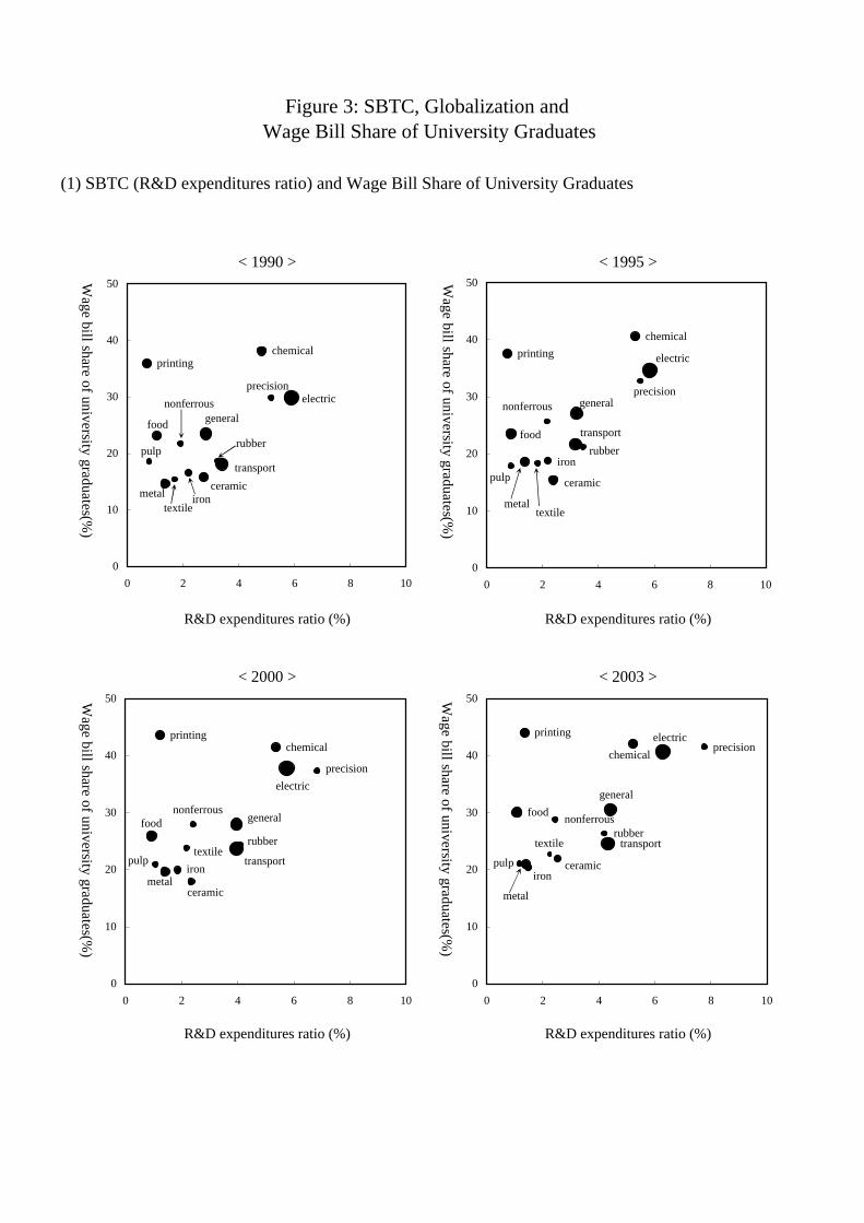
(1) SBTC (R&D expenditures ratio) and Wage Bill Share of University Graduates

< 1990 > < 1995 >

R&D expenditures ratio (%) R&D expenditures ratio (%)

< 2000 > < 2003 >

R&D expenditures ratio (%) R&D expenditures ratio (%)

Figure 3: SBTC, Globalization and Wage Bill Share of University Graduates

printingchemical

food

textile

pulprubber

ceramiciron

nonferrous

metal

general

electric

transport

precision

0

10

20

30

40

50

0 2 4 6 8 10

Wage bill share of university graduates(%

)

printingchemical

food

textile

pulp

rubber

ceramic

iron

nonferrous

metal

general

electric

transport

precision

0

10

20

30

40

50

0 2 4 6 8 10

food

printing

rubbernonferrous

transporttextile

pulp

chemical

ceramiciron

metal

general

electricprecision

0

10

20

30

40

50

0 2 4 6 8 10

printingchemical

food

textilepulp

rubber

ceramic

iron

nonferrous

metal

general

electric

transport

precision

0

10

20

30

40

50

0 2 4 6 8 10

Wage bill share of university graduates(%

)

Wage bill share of university graduates(%

)

Wage bill share of university graduates(%

)

(2) Globalization (Import Ratio from East Asia) and Wage Bill Share of University Graduates

< 1990 > < 1995 >

Import ratio from East Asia (%) Import ratio from East Asia (%)

< 2000 > < 2003 >

Import ratio from East Asia (%) Import ratio from East Asia (%)

Figure 3: (continued)

Notes.1. The size of corresponds to the number of male workers in each industry (Larger indicates that more male workers are employed in the industry).2. Each industry's wage bill share of university graduates is calculated according to the following definition (Every calculation is confined to male workers). (Wage bill share of univ. graduates) = (Wage bill of univ. graduates) / (Total wage bill) 100 where, (Wage bill of univ. graduates) = (Average scheduled cash earnings of univ. graduates) (number of univ. graduates) (Total wage bill) = (Average scheduled cash earnings of all workers) (number of all workers) Sources. Ministry of Health, Labor and Welfare "Basic Survey on Wage Structure, " Ministry of Internal Affairs and Communications "Report on the Survey of Research and Development," Ministry of Economy, Trade and Industry "Census of Manufactures," Cabinet Office "System of National Accounts," Japan Tariff Association "Summary Report on Trade of Japan," Bank of Japan "Corporate Goods Price Index," etc.

×

××

textile

printingchemical

rubbernonferrous

foodpulp

ceramiciron

metal

general

electric

transport

precision

0

10

20

30

40

50

0 5 10 15 20

printingchemical

food

textile

pulp

rubber

ceramic

iron

nonferrous

metal

general

electric

transport

precision

0

10

20

30

40

50

0 5 10 15 20

chemical

rubbernonferrousfood

pulp

printing

ceramic

iron metal

general

electric

transport

precision

0

10

20

30

40

50

0 5 10 15 20

printingchemical

nonferrous

foodpulp

rubber

ceramic

ironmetal

general

electric

transport

precision

0

10

20

30

40

50

0 5 10 15 20

Wage bill share of university graduates(%

)

Wage bill share of university graduates(%

)W

age bill share of university graduates(%)

Wage bill share of university graduates(%

)

(1) University Graduates Ratio

(2) Estimated Time Effects

Figure 4: University Graduates Ratio and Time Effects

16

18

20

22

24

26

1988

1989

1990

1991

1992

1993

1994

1995

1996

1997

1998

1999

2000

2001

2002

2003

(%)

-6

-4

-2

0

2

4

6

1988

1989

1990

1991

1992

1993

1994

1995

1996

1997

1998

1999

2000

2001

2002

2003

Notes.1. University graduates ratio in (1) is the ratio of university graduates and postgraduates to total new graduates (i.e., the sum of primary school, junior high school, high school or junior school under the old system of education, junior college, technical college, university, and postgraduate).2. Time effects in (2) are estimated by two-way fixed effects models (Models (1)-(5) in Table 5(1)).