Chained Financial Frictions and Credit Cycles∗

Federico Lubello† Ivan Petrella‡ Emiliano Santoro§

July 14, 2017

Abstract

We examine the role of bank collateral in shaping credit cycles. To this end, we develop

a tractable model where bankers intermediate funds between savers and borrowers. If

bankers default, savers acquire the right to liquidate bankers’assets. However, due to the

vertically integrated structure of our credit economy, savers anticipate that liquidating

financial assets (i.e., bank loans) is conditional on borrowers being solvent on their debt

obligations. This friction limits the collateralization of bankers’financial assets beyond

that of other assets that are not involved in more than one layer of financial contracting. In

this context, increasing the pledgeability of financial assets eases more credit and reduces

the spread between the loan and the deposit rate, thus attenuating capital misallocation

as it typically emerges in credit economies à la Kiyotaki and Moore (1997). We uncover a

close connection between the collateralization of bank loans, macroeconomic amplification

and the degree of procyclicality of bank leverage. A regulator may reduce macroeconomic

volatility through the introduction of a countercyclical capital buffer, while a fixed capital

adequacy requirement displays limited stabilization power.

JEL classification: E32, E44, G21, G28

Keywords: Banking; Bank Collateral; Liquidity; Capital Misallocation; Macropruden-

tial Policy.

∗We thank– without implicating– Martin Gonzalez Eiras, Søren Hove Ravn, Omar Rachedi, Raffaele Rossiand participants at the “2017 Computation in Economics anf Finance Conference”at Fordham University inNew York for helpful comments and suggestions. Part of this work has been conducted while Santoro wasvisiting Banco de España, whose hospitality is gratefully acknowledged. The views expressed in this paper donot necessarily represent the views of the Banque Centrale du Luxembourg or the Eurosystem.†Banque Centrale du Luxembourg. Address: 2, Boulevard Royal, L-2983 Luxembourg. E-mail : fed-

erico.lubello@bcl.lu.‡Warwick Business School and CEPR. Address: Warwick Business School, The University of Warwick,

Coventry, CV4 7AL, UK. E-mail : Ivan.Petrella@wbs.ac.uk.§Department of Economics, University of Copenhagen. Address: Østerfarimagsgade 5, Building 26, 1353

Copenhagen, Denmark. E-mail : emiliano.santoro@econ.ku.dk.

1

1 Introduction

Lending relationships are typically plagued by information asymmetries that play a major role

in shaping macroeconomic outcomes. In this respect, banks are of central importance, as they

are involved in at least two layers of financial contracting through their intermediation activity

between savers and borrowers. This paper focuses on the macroeconomic implications of banks’

portfolio decisions over different assets in the presence of chained financial frictions, intended as

the combination of collateralized borrowing by both banks and entrepreneurs. To this end, we

devise a tractable model that integrates limited enforceability of loan contracts– as popularized

by Kiyotaki and Moore (1997) (KM, hereafter)– with an analogous friction characterizing the

financial relationship between depositors and bankers. As in recent contributions on banking

and the macroeconomy (see, inter alia, Gertler and Kiyotaki, 2015), deposits are secured by a

fraction of bankers’assets that are pledged as collateral. The main departure from these studies

consists of envisaging different degrees of liquidity– and, thus, pledgeability– for different types

of bank assets. In doing so, our key contribution consists of detailing the mechanisms through

which these collateral assets shape bankers’ incentives to intermediate funds and ultimately

affect the amplitude of business fluctuations.

Financial institutions resort to collateralized debt to raise funds, providing assets as a guar-

antee in case of default on their debt obligations. This is the case for non-traditional banking

activities– with sale and repurchase agreements (repos) employed as a main source of funding–

as well as for commercial banks– where securitized-banking often supplements more traditional

intermediation activities. In fact, banks employ financial collateral both for currency manage-

ment purposes and, more recently, as part of non-standard monetary policy frameworks.1 A

vast literature has focused on quantifying the dynamic multiplier emerging from the limited

enforceability of debt contracts in economies à la KM.2 While most of the contributions in this

tradition have emphasized the role of borrowers’collateral for the amplification of macroeco-

nomic shocks, the role of bank collateral has generally been overlooked.

In our model the ability of bankers to intermediate funds between savers and borrowers

rests on the composition of different assets they are able to pledge as collateral. Along with

extending bank loans, bankers may also invest in an infinitely-lived productive asset, ‘capital’,

whose main purpose is to serve as a buffer against which the intermediary is trusted to be

able to meet its financial obligations. Deposits are bounded from above by bankers’holdings

of both types of collateral assets. However, due to the vertically integrated structure of our

credit economy savers anticipate that, in case of bankers’default, liquidating their financial

claims (i.e., bank loans) is subordinated to borrowers being solvent on their debt obligations.

This friction, which has not been formerly investigated, affects savers’perceived liquidity of

1The set of assets that central banks accept from commercial banks generally includes government bondsand other debt instruments issued by public sectors and international/supranational institutions. In some cases,also securities issued by the private sector can be accepted, such as covered bank bonds, uncovered bank bonds,asset-backed securities or corporate bonds.

2See Kocherlakota (2000), Krishnamurthy (2003) and Cordoba and Ripoll (2004), inter alia.

2

bankers’financial assets beyond that of capital,3 inducing a transaction cost depositors have

to bear in order to liquidate bank loans. If the latter are regarded as relatively illiquid, savers

will be less prone to accept them as collateral.

A key feature of the model is that combining limited enforceability of deposit and loan

contracts reduces the interest rate on loans below the one that would prevail in a standard

economy where only loans are secured by collateral assets. This allows borrowers to extend their

capital holdings, contributing to increase total production in the steady state and alleviating

capital misallocation as it emerges in economies à la KM, where borrowers hold too little capital

in equilibrium, due to constrained borrowing. This property has a striking implication for

equilibrium dynamics: as the propagation of technology shifts crucially rests on the distribution

of real assets between lenders and borrowers, envisaging financially constrained intermediaries

into an otherwise standard KM economy produces a ‘banking attenuator’that is neither linked

to the procyclicality of the external finance premium (Goodfriend and McCallum, 2007), nor to

monopolistic competition and interest rate-setting rigidities in financial intermediation (Gerali

et al., 2010).

The main distinction between different types of bank collateral lies in the way they affect

bankers’ incentives to intermediate funds. Both assets have the potential to relax bankers’

financial constraint. However, while increasing real assets exacerbates capital misallocation

and reduces lending through a negative externality on borrowers’demand for credit, increasing

financial assets compresses the spread between the loan and the deposit rate, thus attenuating

capital misallocation. This feature of the model has key implications for equilibrium dynamics

under different degrees of collateralization of bank loans. A relatively scarce liquidity of bankers’

financial assets amplifies the response of gross output to productivity shocks. As in KM, a

positive technology shift reallocates capital from the lenders to the borrowers. On one hand,

this allows borrowers to expand their borrowing capacity. On the other hand, a decline in

bankers’ real assets is typically counteracted by an expansion in bank loans: as the latter

are perceived to be increasingly illiquid, the compensation effect is gradually muted, so that

bankers need to cut their capital investment further to meet borrowers’higher demand for

credit. In turn, the response of total production– which increases in borrowers’real assets,

ceteris paribus– is amplified, relative to situations in which deposit contracts involve relatively

low transaction costs in case of bankers’default.

The model produces a countercyclical ‘flight to quality’in bankers’optimal asset allocation

(see, e.g., Lang and Nakamura, 1995): during expansions (contractions), bankers increase (de-

crease) their holdings of the inherently riskier assets– bank loans– while decreasing (increasing)

their capital holdings, which do not bear any risk of default. As a result, ‘too much’borrowing

capacity is allocated during boom states and ‘too little’in bad states, inducing a procyclical

bank leverage and generating excessive fluctuations in credit, output and asset prices. From a

normative viewpoint, we study to which extent a hypothetical banking regulator may intervene

to smooth the amplitude of these fluctuations, by impairing the endogenous propagation mech-

3In the remainder we will refer to financial assets and bank loans interchangeably, while capital goods willalso be referred to as real assets.

3

anism of shocks that hinges on capital misallocation. As a matter of fact, a recent orientation in

macroprudential policy-making suggests that– subject to removing or reducing systemic risks

with a view to protecting and enhancing the resilience of the financial system– explicit action

should be taken so as to facilitate the supply of finance for productive investment, thus enhanc-

ing capital allocation (Bank of England, 2016). With reference to our model, we show that a

constant capital-to-asset ratio attenuates the transmission of technology shifts, although the

gap between borrowers’and bankers’marginal product of capital cannot entirely be closed. By

contrast, the regulator may successfully attenuate the economy’s response to the productivity

shock by devising a state-dependent capital buffer that induces a countercyclical bank lever-

age and stabilizes fluctuations in borrowers’collateral, even without resolving the distortion

in capital allocation. This is accomplished by adjusting the capital-to-asset ratio in response

to changes in bank lending: when the rule features enough responsiveness, movements in the

value of borrowers’collateral assets are counteracted by similar-sized changes in the loan rate,

so that the traditional amplification mechanism embodied by borrowers’collateral constraint

is neutralized.

The present paper is strictly related to a growing literature that introduces financial in-

termediation into well established quantitative macroeconomic frameworks, so as to account

for a number of distinctive features of the last financial crisis (see, inter alia, Gertler and

Kiyotaki, 2010). To name a few, Gertler et al. (2012) allow intermediaries to issue outside

equity, thus making risk exposure an endogenous choice of the banking sector, while Gertler

and Kiyotaki (2015) devise a model of banking that allows for liquidity mismatch and bank

runs. More recently, Hirakata et al. (2017) have introduced chained financial contracts into a

dynamic general equilibrium models à la Bernanke et al. (1999).4 The common trait of these

contributions and many others in this tradition is to look at different sources of funding of

financial intermediaries– thus emphasizing the composition of the right-hand side of banks’

balance sheet– while typically considering only one type of asset– bank loans. We deviate

from this approach and focus on the role of limited enforceability of deposit contracts in a

setting where banks may invest in different assets,5 whose distinctive trait is to bear different

degrees of liquidity depending on whether they are involved in more than one layer of financial

relationships.

The paper is also part of a rapidly developing banking literature on the role of macropruden-

tial policy-making. Some recent examples include Martinez-Miera and Suarez (2012), Angeloni

and Faia (2013), Harris et. al (2015), Clerc et. al (2015), Begenau (2015) and Elenev et al.

(2017). These contributions rely on medium- to large-scale dynamic general equilibrium mod-

els. While an obvious advantage of this modeling approach is to allow for a variety of shocks,

transmission channels and alternative policy settings, our framework allows for a neater in-

4Unlike the present framework– which is based on costly enforcement of both deposit and loan contracts–Hirakata et al. (2017) consider costly state verification problems applying to both intermediaries and entrepre-neurs.

5In this respect, our framework is closer to Chen (2001), who stresses the importance of moral hazardbehavior of both bankers and entrepeneurs in a quantitative model à la Holmstrom and Tirole (1997). However,in this framework there is no role for liquidity assessment of different types of bank assets.

4

terpretation of the interplay between bank capital requirements, capital misallocation and the

amplitude of credit cycles. In this respect, our framework is more closely related to Gersbach

and Rochet (2016), who show that complete markets do not suffi ciently stabilize credit-driven

fluctuations, thus providing a clear rationale for macroprudential-policy intervention.

The rest of the paper is organized as follows: Section 2 presents the framework; Section

3 discusses the steady-state equilibrium; Section 4 focuses on equilibrium dynamics in the

neighborhood of the steady state and the amplification of shocks to productivity in connection

with the degree of financial collateralization; Section 5 examines the role of macroprudential

policy-making in reducing capital misallocation to smooth macroeconomic fluctuations; Section

6 concludes.

2 Model

The economy is populated by three types of infinitely-lived, unit-sized, agents: savers, bankers

and borrowers.6 There are two layers of financial relationships: savers make deposits to the

bankers, who act as financial intermediaries and extend credit to the borrowers. Two goods

are traded in this economy: a durable asset, ‘capital’, and a non-durable consumption good.

Capital, which is held by both bankers and borrowers, does not depreciate and is fixed in total

supply to one. All agents have linear preferences defined over non-durable consumption. The

remainder of this section provides further details on the characteristics of the actors populating

the economy and their decision rules.

2.1 Savers

Savers are the most patient agents in the economy. In each period, they are endowed with an

exogenous non-produced income. We assume that savers are neither capable of monitoring the

activity of the borrowers, nor of enforcing direct financial contracts with them. As a result,

savers make deposits at the financial intermediaries. The linearity of their preferences implies

that savers are indifferent between consumption and deposits in equilibrium, so that gross

interest rate on savings (deposits), RS, equals their rate of time preference, 1/βS. Savers’

budget constraint reads as:

cSt + bSt = uS +RSbSt−1, (1)

where cSt denotes the consumption of non-durables, bSt is the amount of savings and u

S is an

exogenous endowment.

6The model is a variation of the ‘Credit Cycles’framework of KM.

5

2.2 Borrowers

Borrowers’ability to attract external funding is bounded by the limited enforceability of debt

contracts. In line with Hart and Moore (1994) we assume that, should borrowers default,

bankers acquire the right to liquidate the stock of capital, kBt . Based on the predicted outcomes

of the renegotiation, borrowers are subject to an enforcement constraint. Neither bankers nor

borrowers are able to observe the liquidation value before the actual default, though borrowers

have all the bargaining power in the liquidation process. With probability 1 − ω (ω ∈ [0, 1])

bankers expect to recover no collateral asset after a default, while with probability ω bankers

expect to be able to recover Etqt+1kBt , where Et indicates the rational expectation operator

and qt+1 denotes the capital price at time t+ 1.

To derive the renegotiation outcome, we consider the following default scenarios:

1. Bankers expect to recover Etqt+1kBt . Since bankers can expropriate the whole stock of

capital, borrowers have to make a payment that leaves bankers indifferent between liq-

uidation and allowing borrowers to preserve the stock of collateral assets. This requires

borrowers to make a payment at least equal to Etqt+1kBt , so that the ex-post value of

defaulting for the bankers is:

RBbBt − Etqt+1kBt , (2)

where RB denotes the gross loan rate and bBt is the loan.

2. Bankers expect to recover no collateral. If the liquidation value is zero, liquidation is

clearly not the best option for the borrowers. Therefore, borrowers have no incentive to

pay the loan back. The ex-post default value in this case is:

RBbBt . (3)

Therefore, enforcement requires that the expected value of non defaulting is not smaller

than the expected value of defaulting, that is:

0 ≥ ω[RBbBt − Etqt+1k

Bt

]+ (1− ω)RBbBt , (4)

which reduces to

RBbBt ≤ ωEtqt+1kBt . (5)

According to (5), the maximum amount of credit borrowers may access is such that the sum

of principal and interest, RBbBt , equals a fraction of the value of borrowers’capital in period

t+ 1.

Borrowers also face a flow-of-funds constraint:

cBt +RBbBt−1 + qt(kBt − kBt−1) = bBt + yBt , (6)

6

where cBt and yBt denote borrowers’consumption and production of perishable goods, respec-

tively. As in KM, borrowers are assumed to combine capital and labor– the latter being

supplied inelastically– through a linear production technology, yBt = αtkBt−1, with αt being a

multiplicative productivity shifter: logαt = ρ logαt−1 + ut, where ρ ∈ [0, 1) and ut is an iid

shock.

Borrowers maximize their utility under the collateral and the flow-of-funds constraints,

taking RB as given. The corresponding Lagrangian reads as:

LBt = E0

∞∑t=0

(βB)t {

cBt − ϑBt[cBt +RBbBt−1 + qt(k

Bt − kBt−1)− bBt − αtkBt−1

](7)

−υt(bBt − ω

qt+1kBt

RB

)},

where βB denotes borrowers’discount factor, while ϑBt and υt are the multipliers associated

with borrowers’budget and collateral constraint, respectively. The first-order conditions are:

∂LBt∂bBt

= 0⇒ −βBRBEtϑBt+1 + ϑBt − υt = 0; (8)

∂LBt∂kBt

= 0⇒ −ϑBt qt + βBEt[ϑBt+1qt+1

]+ βBEt

[ϑBt+1αt+1

]+ ωυtEt

[qt+1

RB

]= 0. (9)

Condition (8) implies that a marginal decrease in borrowing today expands next period’s utility

and relaxes the current period’s borrowing constraint. As for (9), acquiring an additional unit of

capital today allows to expand future consumption not only through the conventional capital

gain and dividend channels, but also through the feedback effect of the expected collateral

value on the price of capital. As we consider linear preferences (i.e., ϑBt = ϑB = 1), (8) implies

υt = υ = 1− βBRB.7 Thus, the collateral constraint binds in the neighborhood of the steady

state as long as RB < 1/βB, which is imposed throughout the rest of the analysis. Finally, (9)

can be rewritten as

qt =βBRB + ω

(1− βBRB

)RB

Etqt+1 + βBEtαt+1. (10)

2.3 Bankers

Bankers’primary activity consists of intermediating funds between savers and borrowers. How-

ever, their ability to attract savers’financial resources is bounded by the limited enforceability

of the deposit contracts, given that bankers may divert assets for personal use (see also Gertler

and Kiyotaki, 2015). At this stage of the analysis we abstract from the implementation of

regulatory bank capital ratios to discourage bankers’moral hazard behavior, while focusing

on the characteristics of the deposit contract. We assume that, upon bankers’default, savers

7Steady-state variables are reported without the time subscript.

7

acquire the right to liquidate bankers’asset holdings.8 At the time of contracting the amount

of deposits, though, the liquidation value of bankers’assets is uncertain. In this respect, the

enforcement problem is isomorphic to that characterizing bankers’ lending relationship with

the borrowers. However, due to the vertically integrated structure of the credit economy, we

envisage an additional friction that limits the pledgeability of bank loans beyond that of cap-

ital. While real assets remain in the availability of the bankers for the entire duration of the

deposit contract– so that savers can frictionlessly liquidate them in case of bankers’default–

the resources corresponding to bankers’financial claims are in the availability of the borrowers.

Therefore, from the perspective of the savers the possibility to liquidate bBt in the event of a

default of the banking sector goes beyond the capacity of the bankers to honor the deposit con-

tract, while being subordinated to borrowers’solvency. In light of this, we assume that savers

account for a transaction cost they would have to bear for seizing bank loans: (1− ξ) bBt , whereξ ∈ [0, 1] indexes savers’perceived liquidity of bankers’financial assets. In the extreme case

savers regard bank loans as completely illiquid and do not accept them as collateral, ξ is set

to zero (i.e., financial frictions are no longer chained), while ξ = 1 corresponds to a situation

in which savers attach no risk to their ability of liquidating financial assets in case bankers’

default.

To derive the renegotiation outcome, we assume that with probability 1− χ savers expectto recover no collateral, while with probability χ the expected recovery value is Etqt+1k

It + ξbBt ,

where kIt denotes bankers’holdings of capital and ξbBt represents the amount of bank loans

held as collateral, net of transaction costs. This implies the following default scenarios:

1. Savers expect to recover Etqt+1kIt + ξbBt . Since savers expect to expropriate the stock of

real and financial assets after bearing a transaction cost (1− ξ) bBt , bankers have to makea payment that leaves savers indifferent between liquidation and allowing borrowers to

preserve the stock of collateral assets. This requires bankers to make a payment at least

equal to Etqt+1kIt + ξbBt , so that the ex-post value of defaulting for the bankers is:

RSbSt − Etqt+1kIt − ξbBt . (11)

2. Savers expect to recover no collateral. If the liquidation value is zero, liquidation is clearly

not the best option for the savers. Therefore, bankers have no incentive to pay deposits

back. The ex-post default value in this case is:

RSbSt . (12)

Enforcement requires that the expected value of not defaulting is not smaller than the

8There are two main considerations why this assumption is a reasonable one: first, savers have no direct useof the collateral assets; second, even if collateral assets represent an attractive investment opportunity, savershave no experience in hedging.

8

expected value of defaulting, so that:

0 ≥ χ[RSbSt − Etqt+1k

It − ξbBt

]+ (1− χ)RSbSt , (13)

which reduces to

RSbSt ≤ χ(Etqt+1k

It + ξbBt

), (14)

according to which deposits should be limited from above by a fraction of the discounted

expected collateral value. Notably, bankers’collateral constraint embodies the notion that real

and financial assets have different degrees of liquidity (see also Bernanke and Gertler, 1985).9

In fact, (14) is reminiscent of the liquidity constraint envisaged by Benigno and Nisticò (2017),

where safe and pseudo-safe assets co-exist and both contribute to set the maximum amount

of resources available for consumption. In their case, while the entire stock of safe assets (i.e.,

money) is available to finance private expenditure, only a fraction of pseudo-safe assets can be

employed to cover consumption, hence displaying less than perfect liquidity.

Some considerations are in order about the role of the capital goods held by the bankers.

First, this asset mainly serves as a buffer against which the intermediary is trusted to be able

to meet its financial obligations.10 In addition, kIt is important in that it breaks the tight

link between deposits and lending– which would be otherwise embodied by a binding deposit

contract– thus allowing for the possibility that a countercyclical ‘flight to quality’drives the

supply of credit. In the present context, such an effect would translate into bankers’allocating

relatively more resources to capital investment– which, unlike bank loans, does not bear any

risk of default– during adverse periods. In turn, this mechanism may open the route to the

emergence of credit crunch episodes (Bernanke and Lown, 1991). Finally, as in Bernanke and

Gertler (1985) we assume that capital is productive, being employed by bankers to invest in

projects on their own behalf.11 Specifically, bankers’ production technology is assumed to

feature the following properties:

yIt = αtG(kIt−1), (15)

9As χ affects the collateralization of both real and financial assets, in the remainder we will refer to ‘financialcollateralization’as the degree of pledgeability of bank loans that is exclusively captured by their liquidity, asindexed by ξ.10Broadly speaking, kIt may be seen as corresponding to bankers’security holdings, which are typically more

liquid, as compared with bank loans.11One can conceive the banking sector as a two-member household sharing externalities and pooling resources.

One member of the household specializes in credit intermediation, whereas the other specializes in production.Therefore, the first household member has to determine the amount of resources to be lent to the borrower,as well as the amount to be extended to the other member of the household. When funds are kept within thehousehold, agency costs are mitigated. Yet, this comes at the cost of bankers-producers accessing a decreasingreturns to scale technology.

9

with G′> 0, G

′′< 0, G

′(0) > % > G

′(1),12 and

% ≡RBβB

[RS(1− βI

)− χ

(1− βIRS

)]RSβI

[RB(1− βB

)− ω

(1− βBRB

)] , (16)

where βI denotes bankers’discount factor and (16) is required to ensure an internal solution

in which both bankers and borrowers demand capital.13

Bankers’flow-of-funds constraint reads as:

cIt + bBt +RSbSt−1 + qt(kIt − kIt−1) = bSt +RBbBt−1 + yIt , (17)

where cIt denotes bankers’consumption. The Lagrangian for bankers’optimization reads as

LIt = E0

∞∑t=0

(βI)t {

cIt − ϑIt [cIt +RSbSt−1 + bBt + qt(kIt − kIt−1) (18)

−bSt −RBbBt−1 − αtG(kIt−1)]− δt(bSt − χ

qt+1

RSkIt − χξ

bBtRS

)},

where ϑIt and δt are the multipliers associated with bankers’budget constraint and enforcement

constraint, respectively. The first-order conditions are:

∂LIt∂bSt

= 0⇒ −RSβIEtϑIt+1 + ϑIt − δt = 0; (19)

∂LIt∂bBt

= 0⇒ RBβIEtϑIt+1 − ϑIt +

1

RSχξδt = 0; (20)

∂LIt∂kIt

= 0⇒ −ϑIt qt + βIEt[ϑIt+1qt+1

]+ βIEt

[ϑIt+1αt+1G

′(kIt )

]+ δtχ

Et [qt+1]

RS= 0. (21)

As we assume linear preferences, ϑIt = ϑI = 1. Therefore, conditions (19) and (20) imply

that the financial constraint holds with equality in the neighborhood of the steady state (i.e.,

δt = δ > 0) as long as (i) RSβI < 1 and (ii) RBβI < 1. Specifically, condition (i) implies that

bankers are relatively more impatient than savers,14 while condition (ii) implies that, unless

either χ or ξ equal zero, bankers charge a lending rate that is lower than their rate of time

preference, as extending loans allows them to relax their financial constraint:

RB =RS − χξ

(1− βIRS

)βIRS

, (22)

12Assuming a decreasing returns to scale technology available to the borrowers would not alter our key results.As we will see in the next section, it is the relatively higher impatience of the borrowers, combined with theircollateral constraint, that endows them with a suboptimal stock of capital. This point is also discussed in KM.Introducing a decreasing returns to scale technology would only hinder the analytical tractability of the model.13The role of this property will be discussed further in Section 4.1.14In this respect, imposing βIRS = 1 reduces the model to the conventional KM economy.

10

from which it is possible to write down the spread between the loan and the deposit rate:

RB −RS =βS − βI

βIβS− χξ 1− βIRS

βIRS. (23)

The first term on the right-hand side of the equality is the spread that would prevail if bankers

could not borrow off their loans (i.e., if χξ = 0), while the second term captures how bankers’

financial constraint affects their ability to intermediate funds. Increasing χ and/or ξ compresses

the spread. As implied by (20), greater pledgeability of financial assets increases the collateral

value that savers expect to recover in case of bankers’ default. This relaxes the financial

constraint, eases more deposits and translates into a higher credit supply, thus compressing

the lending rate.

Although (20) and (21) imply that an increase in either real or financial assets relaxes

borrowers’financial constraint, the distinction between the two types of collateral has crucial

implications for bankers’incentives to intermediate funds between savers and borrowers. On

one hand, while increasing kIt expands bankers’ lending capacity, it also exerts a negative

externality on borrowers’demand for credit by decreasing their collateral. On the other hand,

increasing bBt attenuates the debt-enforcement problem between bankers and borrowers, as

implied by the reduction of the spread between the loan and the deposit rate. As it will be

discussed in Section 4.2, such a distinction has key implications for equilibrium dynamics.

Finally, from (21) we can retrieve the Euler equation governing bankers’investment in real

assets:

qt =RSβI + χ

(1− βIRS

)RS

Etqt+1 + βIEt

[αt+1G

′(kIt )

]. (24)

Note that by relaxing (i) and allowing for βIRS = 1 (i.e., assuming that bankers are as impatient

as savers), (24) reduces to lenders’Euler equation in the conventional direct-credit economy

à la KM. Under these circumstances, bankers are no longer financially constrained. As we

shall see in the next section, this implies both a higher loan rate and a higher user cost of

capital from the perspective of the bankers/lenders, as compared with what observed when

bankers face a binding collateral constraint. These properties will play a crucial role for both

the long-run and the short-run behavior of the model economy.

2.4 Market Clearing

To close the model, we need to state the market-clearing conditions. We know that the total

supply of capital equals one: kIt +kBt = 1. As for the consumption goods market, the aggregate

resource constraint reads as:

yt = yIt + yBt , (25)

where yt denotes the total demand of consumption goods.

11

The aggregate demand and supply for credit are given by the two enforcement constraints

(holding with equality) faced by borrowers and bankers, respectively:

bBt = ωEtqt+1k

Bt

RB, (26)

bBt =1

ξχ

(RSbSt − χEtqt+1k

It

). (27)

Finally, as savers are indifferent between any path of consumption and savings, the amount of

deposits depends on bankers’capitalization. Thus, the markets for deposits and final goods

are cleared according to the Walras’Law.

3 Steady State

Financial frictions characterizing both the savers-bankers relationship and the bankers-borrowers

relationship deeply affect the welfare properties of the model. Examining their interaction in

the long-run is key for understanding the propagation of technology shocks.

In the remainder we impose, without loss of generality, G(kIt−1) =(kIt−1

)µ, with µ ∈ [0, 1].

Evaluating (10) in the non-stochastic steady state returns:

q =RBβB(

1− βB)RB − ω

(1− βBRB

) . (28)

From (24) we retrieve the marginal product of bankers’capital, as a function of its price:

G′(kI) =

RS(1− βI

)− χ

(1− βIRS

)RSβI

q, (29)

so that Equations (28), (29) and kI + kB = 1 pin down borrowers’and bankers’holdings of

capital. In turn, these allow us to characterize the key ineffi ciency at work in the economy.

Importantly, financial collateralization only affects the steady state of the economy through its

impact on RB, which in turn influences the capital price through borrowers’Euler, as implied

by (28).15

[Insert Figure 1]

Figure 1 provides a sketch of the long-run equilibrium of the economy. On the horizontal

axis, borrowers’demand for capital is measured from the left, while bankers’demand from the

right. The sum of the two equals one. On the vertical axis we report the marginal product of

capital of both borrowers and bankers. Borrowers’marginal product of capital is indicated by

the line ACE∗, while bankers’marginal product is represented by the line DE0E∗. The first-

best allocation would be attained at E0, where the product of capital owned by the bankers

and the borrowers is the same, at the margin. In our economy, however, the steady-state

15In light of this, envisaging savers that invest in real assets in place of the bankers would alter neither therole of liquidity of bankers’financial collateral, nor the key aggregate implications of the model.

12

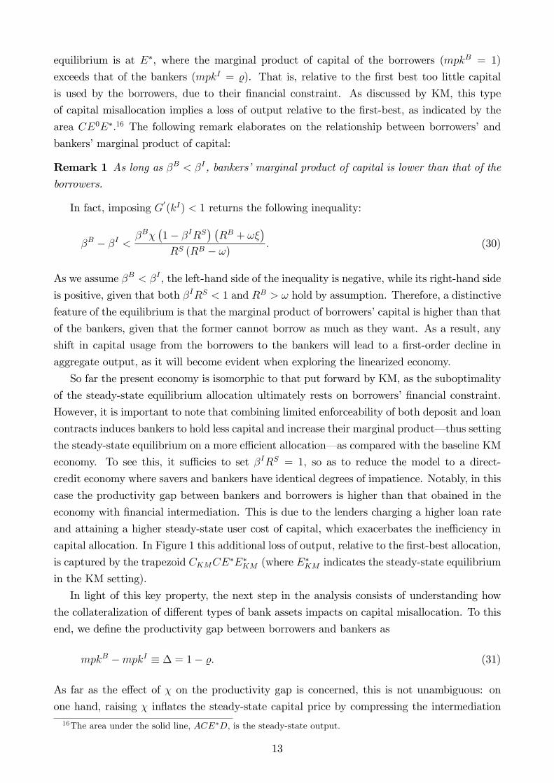
equilibrium is at E∗, where the marginal product of capital of the borrowers (mpkB = 1)

exceeds that of the bankers (mpkI = %). That is, relative to the first best too little capital

is used by the borrowers, due to their financial constraint. As discussed by KM, this type

of capital misallocation implies a loss of output relative to the first-best, as indicated by the

area CE0E∗.16 The following remark elaborates on the relationship between borrowers’and

bankers’marginal product of capital:

Remark 1 As long as βB < βI , bankers’marginal product of capital is lower than that of the

borrowers.

In fact, imposing G′(kI) < 1 returns the following inequality:

βB − βI <βBχ

(1− βIRS

) (RB + ωξ

)RS (RB − ω)

. (30)

As we assume βB < βI , the left-hand side of the inequality is negative, while its right-hand side

is positive, given that both βIRS < 1 and RB > ω hold by assumption. Therefore, a distinctive

feature of the equilibrium is that the marginal product of borrowers’capital is higher than that

of the bankers, given that the former cannot borrow as much as they want. As a result, any

shift in capital usage from the borrowers to the bankers will lead to a first-order decline in

aggregate output, as it will become evident when exploring the linearized economy.

So far the present economy is isomorphic to that put forward by KM, as the suboptimality

of the steady-state equilibrium allocation ultimately rests on borrowers’financial constraint.

However, it is important to note that combining limited enforceability of both deposit and loan

contracts induces bankers to hold less capital and increase their marginal product– thus setting

the steady-state equilibrium on a more effi cient allocation– as compared with the baseline KM

economy. To see this, it suffi cies to set βIRS = 1, so as to reduce the model to a direct-

credit economy where savers and bankers have identical degrees of impatience. Notably, in this

case the productivity gap between bankers and borrowers is higher than that obained in the

economy with financial intermediation. This is due to the lenders charging a higher loan rate

and attaining a higher steady-state user cost of capital, which exacerbates the ineffi ciency in

capital allocation. In Figure 1 this additional loss of output, relative to the first-best allocation,

is captured by the trapezoid CKMCE∗E∗KM (where E∗KM indicates the steady-state equilibrium

in the KM setting).

In light of this key property, the next step in the analysis consists of understanding how

the collateralization of different types of bank assets impacts on capital misallocation. To this

end, we define the productivity gap between borrowers and bankers as

mpkB −mpkI ≡ ∆ = 1− %. (31)

As far as the effect of χ on the productivity gap is concerned, this is not unambiguous: on

one hand, raising χ inflates the steady-state capital price by compressing the intermediation16The area under the solid line, ACE∗D, is the steady-state output.

13

spread, as embodied by (22); on the other hand, a higher χ increases bankers’marginal benefit

of relaxing the collateral constraint by investing into an extra unit of capital, as embodied by

(21): as a result, bankers’have a higher incentive to accumulate capital, so that the first factor

on the right-hand side of (29) decreases in χ. As it will be detailed in the next section, these

competing forces tend to offset each other, so that bankers’deposit-to-value ratio has little

influence on capital misallocation and the propagation of technology disturbances.

As for the pledgeability of bank loans, the following summarizes the impact of financial

collateralization on the productivity gap:

Proposition 1 Increasing the pledgeability of bank loans (ξ) reduces the gap between bankers’and borrowers’marginal product of capital (∆).

Proof. See Appendix A.Notably, a higher degree of financial collateralization expands bankers’ lending capacity

and compresses the spread charged over the deposit rate. In turn, lower lending rates allow

borrowers to increase their borrowing capacity through a higher collateral value, ceteris paribus.

The combination of these effects is such that mpkI unambiguously increases in the degree of

financial collateralization, reducing the productivity gap with respect to the borrowers. This

factor will play a key role in determining the size of the response of gross output to a technology

shock, as it will be detailed in Section 4.1.

4 Equilibrium Dynamics

To examine equilibrium dynamics we preliminarily log-linearize the key behavioral rules and

constraints around the non-stochastic steady state, where the incentive compatibility con-

straints (5) and (14) are assumed to hold with equality.17 This local approximation method is

accurate to the extent that we limit the technology shock to be bounded in the neighborhood

of the steady state, so that neither borrowers’nor bankers’default occurs as an equilibrium

outcome. As for borrowers’Euler equation (10):

qt = φEtqt+1 + (1− φ)Etαt+1, (32)

where φ ≡ βBRB+ω(1−βBRB)RB

. As for the bankers’Euler equation (24):

qt = λEtqt+1 + (1− λ)Etαt+1 +1− λη

kBt , (33)

where λ ≡ RSβI+χ(1−βIRS)RS

and η−1 is the elasticity of the bankers’marginal product of capital

times the ratio of borrowers’to bankers’capital holdings in the steady state (i.e., η ≡ 1−kBkB(1−µ)

).

Once we obtain the solutions for qt and kBt as linear functions of the technology shifter, we

can determine closed-form expressions for the equilibrium path of other variables in the model.

17Variables in log-deviation from their steady-state level are denoted by a "^".

14

We first focus on (32), whose forward-iteration leads to:

qt = γαt, (34)

where γ ≡ 1−φ1−φρρ > 0. With this expression for qt, we can resort to (33), obtaining

kBt = vαt, (35)

where v ≡ η1−λ

(λ−φ)(1−ρ)ρ1−φρ > 0. Thus, it is possible to linearize total production in the neigh-

borhood of the steady state, obtaining:

yt = αt + ∆yB

ykBt−1, (36)

According to (36), the dynamics of gross output is shaped by αt, as well as by borrowers’

capital holdings at time t − 1: the second effect captures the endogenous propagation of pro-

ductivity shifts on gross output. In fact, yt depends on the past history of shocks not only

through the first-round impact of αt, but also through the effect of αt−1 on kBt−1, as implied by

(35). In light of this, we can rewrite (36) as

yt = $αt−1 + ut (37)

where$ ≡ ρ+v∆yB

y. According to (37), eliminating the key source of steady-state ineffi ciency–

i.e., attaining ∆ = 0– implies that total output’s departures from the steady state would track

the path of the technology shock, so that the model would feature no endogenous propagation

of productivity shifts.18 Moreover, we need to recall that envisaging limited enforceability of

both deposit and loan contracts reduces capital misallocation as it emerges in the original KM

economy, thus compressing ∆ with respect to the case in which RSβI = 1. In this respect, the

model produces a ‘banking attenuator’that entirely rests on the functioning of financial fric-

tions in banking activity, as compared with analogous effects stemming from the procyclicality

of the external finance premium (Goodfriend and McCallum, 2007) or monopolistic competi-

tion in the intermediation activity and staggered interest rate-setting schemes (Gerali et al.,

2010).

4.1 Financial Collateral and Macroeconomic Amplification

We have now lined up the elements necessary to examine how savers’perceived liquidity of

bankers’financial assets affects the amplitude of credit cycles. In this respect, there are three

different channels through which ξ affects the endogenous response of total production to a

18This property echoes the role of the steady-state ineffi ciency for short-run dynamics in the KM model.In their setting, closing the gap between lenders’and borrowers’marginal product of capital would imply noresponse at all to a productivity shift. In this respect, the key difference between the two frameworks lies inthat we assume an autoregressive shock, while they consider an unexpected one-off shift in technology.

15

technology shock:

∂$

∂ξ= ∆

yB

y

∂v

∂ξ+ v

yB

y

∂∆

∂ξ+ v∆

∂(yB/y

)∂ξ

. (38)

As for the first term on the right hand side of (38), Proposition 2 details the effect induced

by a marginal change in the degree of financial collateralization on the response of borrowers’

capital holdings to the technology shock.

Proposition 2 Increasing the degree of collateralization of bank loans (ξ) attenuates the impactof the technology shock on both borrowers’holdings of capital and the capital price.

Proof. See Appendix A.According to Proposition 2 the sensitivity of borrowers’capital holdings to the technology

shifter decreases in ξ. The intuition for this is twofold: first, increasing ξ determines a more

even distribution of capital goods, as reflected by the drop in η; second, being able to pledge a

higher share of financial assets reinforces the sensitivity of the capital price to the capital gain

component in borrowers’Euler equation, φ, through the drop in the loan rate, while reducing

the sensitivity to the dividend component (i.e., the shock). These effects are mutually reinforc-

ing and ultimately exert a negative force on the overall degree of macroeconomic amplification

of the system.

Turning our attention on the other two terms on the right hand side of (38), we know from

Proposition 1 that the productivity gap between borrowers and bankers shrinks as financial

collateralization increases (i.e., ∂∆/∂ξ < 0). Finally, it is immediate to prove that the last

term on the right-hand side of (38) is positive, in light of greater collateralization of bank loans

inducing a reallocation of capital from the bankers to the borrowers. In turn, this transfer

implies both a first-order positive effect on yB and a (milder) second-order positive impact on

y, so that the overall effect on yB/y is positive.19

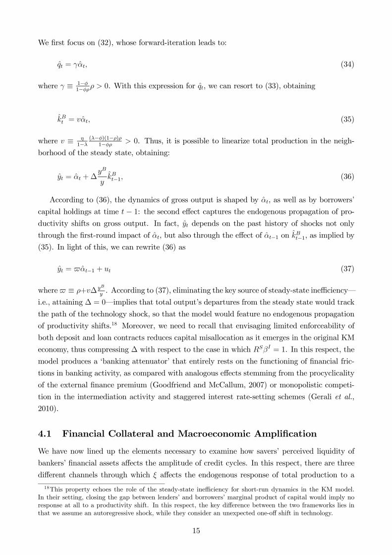
[Insert Figure 2]

To sum up, an increase in ξ causes competing effects on $. First, greater financial collater-

alization depresses the pass-through of αt−1 on borrowers’capital holdings, which in turn affect

total production with a lag. Second, raising ξ exerts two distinct effects on the pass-through of

kBt−1 on yt: on one hand, bankers’marginal product of capital increases, implying a reduction of

the productivity gap; on the other hand, borrowers’contribution to total production increases,

as the reduction in the productivity gap reflects higher capital accumulation in the hands of

the borrowers. The sum of these three forces potentially leads to mixed results on output

amplification, as captured by the second-round effect of technology disturbances. To address

19Recall that total output is an increasing function of borrowers’capital. Therefore, the drop in yI followinga marginal increase in ξ is lower than the corresponding rise in yB .

16

this, we plot $ as a function of ξ and µ.20 The aim of this exercise is to examine the direction

of the overall effect exerted by financial collateralization on macroeconomic volatility, rather

than quantifying an empirically plausible multiplier emerging from the interaction of bankers’

and borrowers’financial constraints.21 As it emerges from Figure 2, increasing ξ compresses

$, at any level of µ. By contrast, increasing the income share of capital in bankers’production

technology amplifies the second-round response of output. This is because µ amplifies the pro-

ductivity gap through its positive effect on η.22 All in all, the general picture emerging from

this exercise is that allowing for greater financial collateralization attenuates the overall degree

of amplification of technology disturbances. The next subsection examines how this property

reflects into cyclical movements in bank leverage, whose behavior is key to understanding how

bankers’balance sheet affects the amplitude of credit cycles.

4.2 The Role of Leverage

To enlarge our perspective on the amplification/attenuation induced by bankers’financial col-

lateral, we take a closer look at their balance sheet. To this end, we define bankers’equity

as the difference between the value of total assets (i.e., loans and capital) and liabilities (i.e.,

deposits):

eIt = bBt + qtkIt − bSt , (39)

with leverage defined as the ratio between loans and equity: levIt = bBt /eIt .

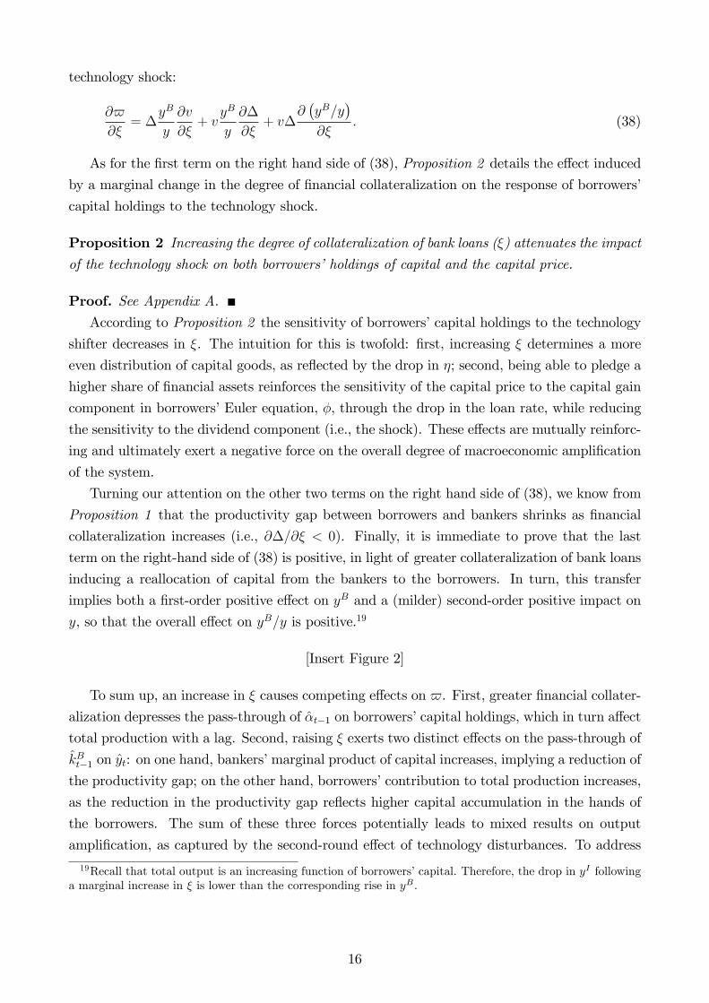
Figure 3 reports the response of selected variables to a one-standard deviation shock to

technology.23 As implied by (36), on impact output responds one-to-one with respect to the

shock, regardless of the degree of financial collateralization. However, as ξ increases the second-

round response is gradually muted. To complement our analytical insight and provide further

20The discount factors are set in accordance with our assumptions about the relative degree of impatienceof the three agents in the economy and are broadly in line with existing (quarterly) calibrations involvingeconomies with heterogeneous agents: βS = 0.99, βI = 0.98, βB = 0.97. We set ρ = 0.95, in line with theempirical evidence showing that technology shocks are generally small, but highly persistent (see, e.g., Cooleyand Prescott, 1995). As for χ and ω , they are both set to 1, so as to ensure a wider set of admissible combinationsof ξ and µ that correspond to positive holdings of capital for both bankers and borrowers. This is clearlydisplayed by the robustness evidence reported in Appendix C, which shows that different combinations of χand ω are close to irrelevant regarding the effect of financial collateralization on macroeconomic amplification.Moreover, Figure C1 shows that varying χ has virtually no effect on the amplitude of the response to thetechnology shock, in light of the competing effects exerted on bankers’marginal product of capital.21We leave this task for future research employing a large-scale dynamic general equilibrium model.22It is important to emphasize that increasing µ may violate the condition G

′(0) > % > G

′(1), which ensures

an interior solution as for how much capital bankers should hold in the neighborhood of the steady state. Tosee why this is the case, recall that µ

(kI)µ−1

= %. Increasing µ inflates bankers’marginal product of capital,while leaving their user cost unaffected: Thus, as µ increases bankers are induced to hold an increasing stockof capital, so that the equality holds. An important aspect is that this effect tends to kick in earlier as ξdeclines. This is because a drop in the degree of financial collateralization depresses bankers’ user cost ofcapital. Therefore, as ξ declines and µ increases the set of steady-state allocations in which both bankers andborrowers hold capital restricts, as the condition % > G

′(1) is eventually violated and borrowers’may virtually

end up with negative capital holdings.23The baseline parameterization is the same as that employed in Figure 2. As for µ, we impose a rather

conservative value, 0.4, which allows us to obtain a finite distribution of capital in the steady state.

17

intuition on this channel, we examine the behavior of a set of variables involved in bankers’

intermediation activity. In this respect, note that deposits tend to decline at low values of

ξ, while increasing as bankers can pledge a higher share of their financial assets. The reason

for this can be better understood by recalling the nature of the interaction between bankers’

financial and real assets. The interplay takes place on two levels: on one hand, both assets have

a positive effect on savers’deposits, as embodied by (14); on the other hand, it is possible to

uncover a crowding out effect, as increasing bankers’real asset holdings exerts a negative force

on lending by reducing borrowers’collateral. How do these properties affect the transmission

of an expansionary technology shock? Due to the capital productivity gap between borrowers

and bankers, the technology shift necessarily causes a decline of bankers’ real assets, thus

expanding borrowers’capital and borrowing.24 Therefore, in equilibrium deposits are influenced

by two opposite forces, namely an expansion in the amount of bankers’financial assets and a

contraction in their stock of real assets. In this respect, the implied allocation of bankers’assets

reflects a countercyclical flight to quality pattern (see, inter alia, Lang and Nakamura, 1995):

during expansions (contractions), bankers increase (decrease) their holdings of the inherently

riskier assets– bank loans– while decreasing (increasing) their capital holdings, which do not

bear any risk of default.

[Insert Figure 3]

How do these diverging forces translate in terms of bankers’ability to attract deposits and

leverage? As ξ drops the impact of bank loans is gradually muted and deposits eventually

track the dynamics of bankers’capital. In this context, the contraction of bankers’real asset

overcomes the drop in deposits, so that lending expands in excess of bank equity, potentially

leading to an increase in leverage. In fact, a procyclical leverage ratio is associated with a

relevant degree of macroeconomic amplification, when bankers’financial assets are regarded

as relatively illiquid. Figure 3 shows this tends to be the case for ξ < 0.5, under our baseline

parameterization.

5 Welfare and Capital Adequacy Requirements

The positive analysis so far has shown that limited enforceability of deposit contracts may

reduce the productivity gap between borrowers and lenders, which is key to quantify the am-

plitude of credit cycles. In light of this, our next objective is to understand to which extent

a regulator may promote a more effi cient allocation of productive capital by ‘leaning against’

capital misallocation. In this respect, the Chancellor of the Exchequer has explicitly indicated

that– conditional on enhancing the resilience of the financial system– the Financial Policy

24This is a distinctive feature of lender-borrower relationships involving the collateralization of a productiveasset. In fact, it is possible to show that, following a positive technology shock, the major reallocation of landfrom the lenders to the borrowers is only attenuated by relaxing the hypothesis of zero aggregate investment —as in the KM baseline framework —while the direction of the transfer is not inverted.

18

Committee at the Bank of England should intend the pursual of productive capital allocation

effi ciency as part of its macroprudential-policy mandate:

"Subject to achievement of its primary objective, the Financial Policy Committee

(FPC) should support the Government’s economic objectives by acting in a way that,

where possible, facilitates the supply of finance for productive investment provided

by the UK’s financial system." (Remit and Recommendations for the Financial

Policy Committee, HM Treasury, July 8, 2015).

In fact, our economy lends itself to the analysis of this particular problem, in light of

the strict connection between the capital productivity gap between borrowers and bankers

and the amplitude of credit cycles.25 To this end, we introduce two complementary tools of

regulation. First, we assume deposit insurance, which ensures that savers do not suffer a loss

in the event of bankers’default.26 A direct implication of such a measure is to shift the risk

of bankers’default to the government (or a hypothetical interbank deposit protection fund),

so that the renegotiation of deposit contracts is redundant and bankers’financial constraint

may be discarded. However, in order to mitigate bankers’moral hazard behavior, the regulator

imposes an explicit capital adequacy requirement (see, e.g., Van den Heuvel, 2008). According

to this regulatory constraint, equity needs to be at least a fraction θ of the loans, for bankers

to be able to operate:

eIt ≥ θbBt , θ ∈ [0, 1] , (40)

where θ denotes the capital-to-asset ratio.

Appendix B reports bankers’optimization problem under (40). In this case, the equilibrium

loan rate reads as

RB =RS − (1− θ)

(1− βIRS

)βI

. (41)

Notably, (41) is isomorphic to (22), with RB increasing in the capital-to-asset ratio. To provide

an intuition for this, we combine (40) with (39), obtaining:

bSt ≤ qtkIt + (1− θ) bBt . (42)

As embodied by (42), imposing a capital-to-asset ratio to bankers’ intermediation activity

amounts to constrain deposits from above by the current value of bankers’collateral, with the

25Notably, our model abstracts from trade-offs that impose the policy-maker to balance the incentive toimprove the allocation of productive capital with an alternative financial stability objective, as in Gertler andKiyotaki (2015), inter alia. However, our primary interest is to understand how far the policy-maker can goso as to resolve the key distortion in the credit economy, so that there is no need to introduce additionalpropagation mechanisms that would only hinder the analytical tractability of the model.26As in Van den Heuvel (2008), deposit insurance is left unmodeled, though it is argued that it generally

improves banks’ability to extend credit (see Diamond and Dybvig, 1983).

19

implied degree of pledgeability of bank loans being a negative function of θ. In fact, there is a

direct mapping between the capital-to-asset ratio implicit in the capital requirement constraint

imposed by the regulator and the degree of collateralization of bank loans as it emerges from

the incentive compatibility constraint (14), which is derived in the absence of any form of

deposit insurance. Intuitively, a higher leverage (lower capital) ratio implies a riskier exposure

of the financial intermediary. This translates into greater transaction costs savers would have

to bear in order to seize bank loans in the event of bankers’default. In turn, these costs have a

direct impact on degree of collateralization of bankers’financial assets that is implicit in (40).

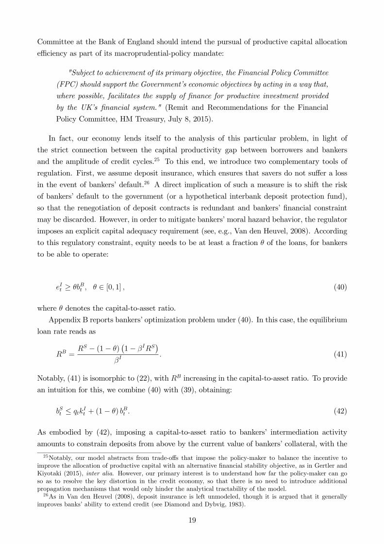
[Insert Figure 4]

Therefore, it should come as no surprise that, absent any trade-offbetween enhancing capital

allocation and ensuring financial stability, the optimal policy consists of setting the capital-to-

asset ratio to its lower bound. Along with minimizing the fraction of bank assets that can be

financed by issuing deposit liabilities, θ = 0 contracts the intermediation spread, thus ensuring

a more effi cient allocation of capital between bankers and borrowers. Figure 4– which reports

the response of the economy to a positive technology shock under this policy– confirms this

view. Nevertheless, it is important to notice that even a null capital ratio is not enough to

neutralize the endogenous propagation channel stemming from capital misallocation, as stated

by the next proposition.

Proposition 3 The gap between bankers’and borrowers’marginal product of capital (∆) can-not be closed by setting the capital-to-asset ratio (θ) within the range of admissible values.

Proof. See Appendix A.To dig deeper on this property, Figure 5 maps the spread between the loan and the deposit

rate (y-axis) and the productivity gap (x-axis), for different values of the capital-to-asset ratio

(θ) and the loan-to-asset ratio applying to the borrowers (ω). As we move down along each

locus, θ decreases from its upper bound to the value consistent with ∆ = 0. The color of

a given line switches from green to blue when θ drops below its lower bound. In line with

Proposition 3, closing the productivity gap through a capital requirement within the set of

its admissible values proves to be infeasible for the policy maker. However, it is important

to acknowledge that higher loan-to-value ratios applying to the loan contracts compress the

productivity gap at any value of θ. In fact, raising ω relaxes borrowers’collateral constraint,

allowing them to increase their capital holdings, so that bankers’marginal product of capital

increases in equilibrium.

[Insert Figure 5]

Figure 5 also shows that ∆ = 0 may only be attained at negative values of θ and RB −RS.

In Figure 4– where the capital-to-asset ratio compatible with a null productivity gap is denoted

by θ∆=0– the endogenous propagation of the shock is actually switched off under a negative

capital-to-asset ratio, so that gross output tracks the dynamics of the productivity shifter and

20

leverage is completely acyclical. However, according to (40), setting θ = θ∆=0 would induce

bankers to hold negative equity, for any level of credit extended. Although we rule this out as an

equilibrium outcome, it is interesting to briefly examine the underlying incentives of the bankers

in such a scenario: according to (42), through a negative capital-to-asset ratio, the regulator

implicitly pushes for an ‘hyper-collateralization’of bank loans. In turn, this eventually induces

bankers to set a loan rate below the interest rate on deposits, which amounts to subsidizing

borrowers’capital investment so as to resolve the distortion.

5.1 A Countercyclical Capital Buffer

The normative analysis so far has shown that imposing a constant capital requirement plays a

limited role in smoothing economic fluctuations. Thus, we turn our attention to an alternative

regulatory measure that aims at reducing gross output fluctuations by affecting the cyclicality

of bankers’balance sheet, without necessarily tackling the distortion stemming from capital

misallocation. To this end, recent years have witnessed an increasing interest of policymakers

towards leaning against credit imbalances, pursuing macroeconomic stabilization through pol-

icy rules that set a countercyclical capital buffer. De facto, countercyclical capital regulation

is a key block of the Basel III international regulatory framework for banks.27 Based on the

analysis of the transmission mechanism and the response of bank capital, we now examine

the functioning of this type of policy tool within our framework. Thus, we allow for capital

requirements to vary with the macroeconomic conditions (see, e.g., Angeloni and Faia, 2013,

Nelson and Pinter, 2016 and Clerc et al., 2015):

θtθ

=

(bBtbB

)ϕ, ϕ ≥ 0, (43)

where ϕ = 0 implies a constant capital-to-asset ratio, while ϕ > 0 induces a countercyclical

capital buffer.28

By linearizing the time-varying counterpart of (41) in the neighborhood of the steady state

we obtain:

RBt = ψθt, (44)

where ψ = 1−βIRSβIRB

θ is positive, in light of assuming βIRS < 1. We then linearize (43), obtaining:

θt = ϕbBt . (45)

27The regulatory framework evolved through three main waves. Basel I has introduced the basic capitaladequacy ratio as the foundation for banking risk regulation. Basel II has reinforced it and allowed banks touse internal risk-based measure to weight the share of asset to be hold. Basel III has been brought in responseto the 2007-2008 crisis, with the key innovation consisting of introducing countercyclical capital requirements,that is, imposing banks to build resilience in good times with higher capital requirements and relax them duringbad times.28According to the Basel III regime, capital regulation can respond to a wide range of macroeconomic

indicators. Here we assume it to respond to deviations of bBt from its long-run equilibirum, bB .

21

After linearizing borrowers’financial constraint, we can substitute for bBt in (45) and plug the

resulting expression into (44), so as to obtain:

RBt =

ψϕ

1 + ψϕ

(Etqt+1 + kBt

). (46)

Thus, it is possible to establish a connection between the loan rate and borrowers’expected

collateral value. Increasing the responsiveness of the capital-to-asset ratio to changes in aggre-

gate lending amplifies this channel: raising ϕ implies that marginal deviations of bBt from its

steady state transmit more promptly to the capital-to-asset ratio and, in turn, to the loan rate

through the combined effect of (44) and (45). This induces a feedback effect on borrowers’ca-

pacity to attract external funding, as embodied by their collateral constraint: higher sensitivity

of the loan rate to variations in aggregate lending (i.e., a steeper loan supply function) implies

stronger discounting of borrowers’expected collateral. In the limit (i.e., as ϕ → ∞) there isa perfect pass-through of Etqt+1 + kBt on R

Bt . Therefore, as in the face of a technology shock

both terms move in the same direction and by the same extent, borrowing does not deviate

from its steady-state level and output displays no endogenous propagation.

[Insert Figure 6]

To assess the stabilization performance of the countercyclical capital buffer rule, in Figure

6 we set the steady-state capital-to-asset ratio to 8%– in line with the full weight level of Basel

I and the treatment of non-rated corporate loans in Basel II and III– while varying ϕ over the

support [0, 1].29 As expected, at ϕ = 0 (i.e., a capital-to-asset ratio kept at its steady-state

level) we observe the strongest amplification of the output response, while the lending rate

and bank leverage are both acyclical. By contrast, increasing the degree of countercyclicality

of the capital buffer proves to be effective at attenuating the response of gross output to

the shock, progressively compressing bank leverage. Notably, as ϕ → ∞ leverage displays

a strong degree of countercyclicality,30 while lending does not deviate from its steady-state

level, as conjectured above. In turn, this results in the response of gross output featuring no

endogenous propagation of technology shocks, despite the regulator’s policy action is not aimed

at tackling capital misallocation and, therefore, the steady-state productivity gap is not closed.

6 Concluding Remarks

We have devised a credit economy where bankers intermediate funds between savers and bor-

rowers, assuming that bankers’ability to collect deposits is affected by limited enforceability:

as a result, if bankers default, savers acquire the right to liquidate bankers’asset holdings. In

29Alternative values of θ would only alter the quantitative implications of the exercise, while not affecting itskey qualitative result.30This is accomplished by setting ϕ = 10, meaning that, for a 1% deviation of debt from its steady-state

level, the capital-to-asset ratio is adjusted from its 8% steady-state level up to 8.8%.

22

this context, we have examined the role of bank loans as a form of collateral in deposit con-

tracts. Due to the structure of our credit economy, which may well account for different forms

of financial intermediation, savers anticipate that liquidating financial assets is conditional on

borrowers being solvent on their debt obligations. This friction limits the degree of collat-

eralization of bankers’financial assets beyond that of capital. We have demonstrated three

main results: i) limited enforceability of deposit contracts counteracts the effects of limited

enforceability of loan contracts, thus reducing capital misallocation as it emerges in KM; ii)

greater collateralization of bankers’financial assets dampens macroeconomic fluctuations by

reducing the degree of procyclicality of bank leverage; iii) while imposing a fixed capital-to-

asset ratio to the bankers cannot fully neutralize capital misallocation and enhance a more

effi cient allocation of productive capital– thus switching off the associated endogenous propa-

gation channel of productivity shock– a countercyclical capital adequacy requirement proves

to be rather effective at smoothing credit cycles.

Our model is necessarily stylized, though it can be generalized along a number of dimensions.

For instance, a realistic extension could consist of allowing bankers to issue equity (outside eq-

uity), so as to evaluate how a different debt-equity mix may affect macroeconomic amplification

over expansions– when equity can be issued frictionlessly– and contractions, when equity is-

suance may be precluded due to tighter information frictions. This factor should counteract

the role of financial assets and help obtaining a countercyclical leverage. In connection with

this point, we could also allow for occasionally binding financial constraints, so as to evalu-

ate how the policy-maker should behave across contractions– when constraints tighten– and

expansions, when constraints may become non-binding. However, as this type of extensions

necessarily hinder the analytical tractability of our problem, we leave them for future research

projects based on large-scale models.

23

Figure 1: Steady-state equilibrium

Figure 2: Business cycle amplification

Notes. Figure 2 graphs $ as a function of ξ and µ, under the following parameteriza-tion: βS= 0.99, βI= 0.98, βB= 0.97, ρ = 0.95, χ = ω = 1. The white area denotes inadmissibleequilibria where bankers’capital holdings are virtually negative.

24

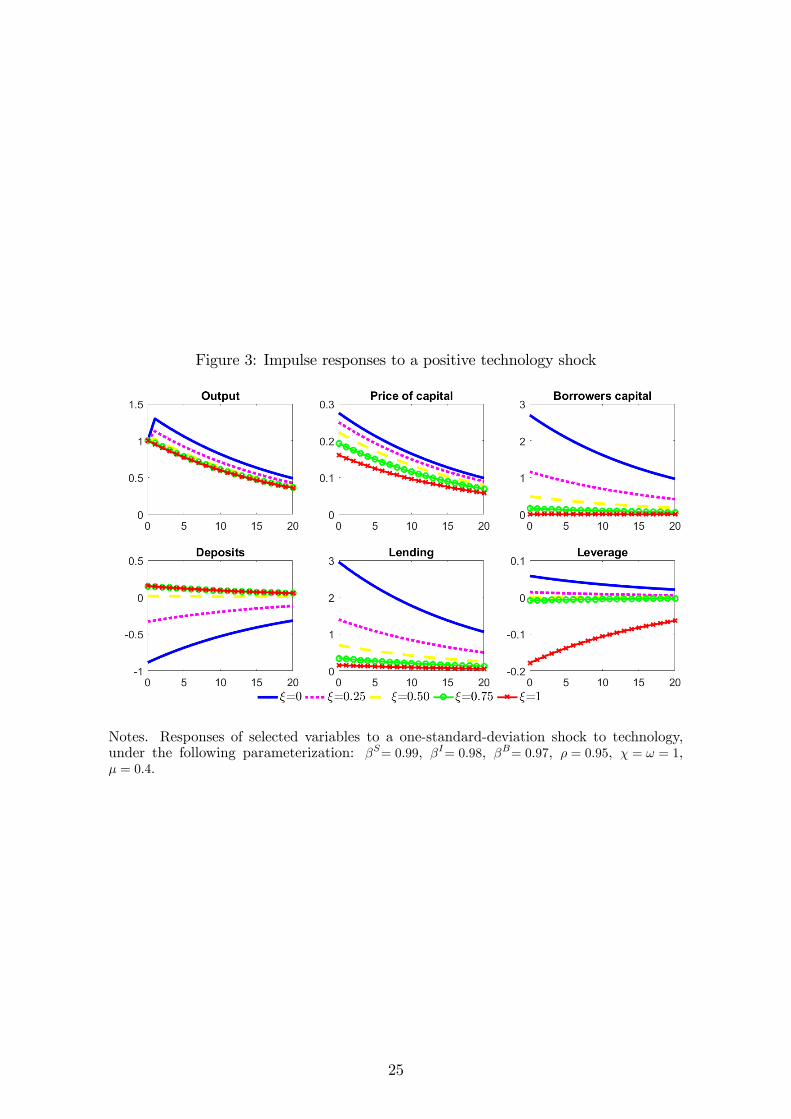
Figure 3: Impulse responses to a positive technology shock

Notes. Responses of selected variables to a one-standard-deviation shock to technology,under the following parameterization: βS= 0.99, βI= 0.98, βB= 0.97, ρ = 0.95, χ = ω = 1,µ = 0.4.

25

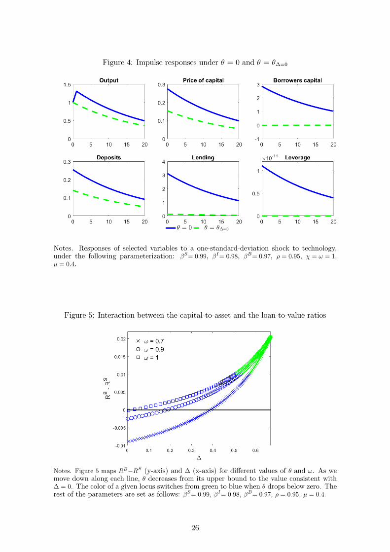
Figure 4: Impulse responses under θ = 0 and θ = θ∆=0

Notes. Responses of selected variables to a one-standard-deviation shock to technology,under the following parameterization: βS= 0.99, βI= 0.98, βB= 0.97, ρ = 0.95, χ = ω = 1,µ = 0.4.

Figure 5: Interaction between the capital-to-asset and the loan-to-value ratios

Notes. Figure 5 maps RB−RS (y-axis) and ∆ (x-axis) for different values of θ and ω. As wemove down along each line, θ decreases from its upper bound to the value consistent with∆ = 0. The color of a given locus switches from green to blue when θ drops below zero. Therest of the parameters are set as follows: βS= 0.99, βI= 0.98, βB= 0.97, ρ = 0.95, µ = 0.4.

26

Figure 6: Impulse responses under different ϕs

Notes. Responses of selected variables to a one-standard-deviation shock to technology,under the following parameterization: βS= 0.99, βI= 0.98, βB= 0.97, ρ = 0.95, χ = ω = 1,µ = 0.4, θ = 0.08.

27

References

[1] Angeloni, I. and E. Faia, 2013, Capital Regulation and Monetary Policy with Fragile

Banks, Journal of Monetary Economics, 60:311—324.

[2] Bank of England, 2016, Understanding and Measuring Finance for Productive Investment,

Discussion Paper.

[3] Begenau, J., 2015, Capital Requirements, Risk Choice, and Liquidity Provision in a Busi-

ness Cycle Model, mimeo, Harvard Business School.

[4] Benigno, P. and S. Nisticò, 2017, Safe Assets, Liquidity and Monetary Policy, American

Economic Journal: Macroeconomics, 9:182—227.

[5] Bernanke, B.S. and M. Gertler, 1985, Banking in General Equilibrium, NBER Working

Papers 1647, National Bureau of Economic Research, Inc.

[6] Bernanke, B. S., M. Gertler and S. Gilchrist, 1999, The Financial Accelerator in a Quan-

titative Business Cycle Framework, in Handbook of Macroeconomics, J. B. Taylor and M.

Woodford (eds.), Vol. 1, chapter 21:1341—1393.

[7] Bernanke, B.S. and C. S. Lown, 1991, Credit Crunch, Brookings Papers on Economic

Activity, 22:205—248.

[8] Chen, N.-K., 2001, Bank Net Worth, Asset Prices and Economic Activity, Journal of

Monetary Economics, Elsevier, 48:415—436.

[9] Clerc, L., A. Derviz, C. Mendicino, S. Moyen, K. Nikolov, L. Stracca, J. Suarez and A. P.

Vardoulakis, 2015, Capital Regulation in a Macroeconomic Model with Three Layers of

Default, International Journal of Central Banking, 11:9—63.

[10] Cooley, T. F. and E. C. Prescott, 1995, Economic Growth and Business Cycles. Princeton

University Press.

[11] Cordoba, J. C. and M. Ripoll, 2004, Credit Cycles Redux, International Economic Review,

45:1011—1046.

[12] Diamond, D. W. and P. H. Dybvig, 1983, Bank Runs, Deposit Insurance, and Liquidity,

Journal of Political Economy, 91:401—419.

[13] Elenev. V., T. Landovoigt and S. Van Nieuwerburgh, 2017, A Macroeconomic Model with

Financially Constrained Producers and Intermediaries, SSRN Library.

[14] Gerali, A., S. Neri, L. Sessa and F.M. Signoretti, 2010, Credit and Banking in a DSGE

Model of the Euro Area, Journal of Money, Credit and Banking, 42:107—141.

[15] Gersbach, H. and J.-C. Rochet, 2016, Capital Regulation and Credit Fluctuations, forth-

coming, Journal of Monetary Economics.

28

[16] Gertler, M. and N. Kiyotaki, 2010, Financial Intermediation and Credit Policy in Business

Cycle Analysis, Handbook of Monetary Economics, in: Benjamin M. Friedman & Michael

Woodford (ed.), 3:547—599.

[17] Gertler, M. and N. Kiyotaki, 2015, Banking, Liquidity, and Bank Runs in an Infinite

Horizon Economy, American Economic Review, 105:2011—2043.

[18] Gertler, M., N. Kiyotaki and A. Queralto, 2012, Financial Crises, Bank Risk Exposure

and Government Financial Policy, Journal of Monetary Economics, 59:17—34.

[19] Goodfriend, M. and B.T. McCallum, 2007, Banking and Interest Rates in Monetary Policy

Analysis: a Quantitative Exploration, Journal of Monetary Economics, 54:1480—1507.

[20] Harris, M., C. C. Opp and M. M. Opp, 2014, Macroprudential Bank Capital Regulation

in a Competitive Financial System, mimeo, University of California, Berkeley (Haas).

[21] Hart, O. and J. Moore, 1994, A Theory of Debt Based on the Inalienability of Human

Capital, Quarterly Journal of Economics 109:841—879.

[22] Hirakata, N., N. Sudo and K. Ueda, 2009, Chained Credit Contracts and Financial Accel-

erators, forthcoming, Economic Inquiry.

[23] HM Treasury, 2015, Remit and Recommendations for the Financial Policy Committee, 8

July.

Available at http://www.bankofengland.co.uk/financialstability/Documents/fpc/letters

[24] Holmstrom, B. and J. Tirole, 1997, Financial Intermediation, Loanable Funds and the

Real Sector, Quarterly Journal of Economics 112:663—691.

[25] Kiyotaki, N. and J. Moore, 1997, Credit Cycles, Journal of Political Economy, 105:211—

248.

[26] Kocherlakota, M. R., 2001, Risky Collateral and Deposit Insurance, The B.E. Journal of

Macroeconomics, 1:1—20.

[27] Krishnamurthy, A., 2003, Collateral Constraints and the Amplification Mechanism, Jour-

nal of Economic Theory, 111:277—292.

[28] Lang, W. and L. Nakamura, 1995, Flight to Quality in Banking and Economic Activity,

Journal of Monetary Economics, 36:145—164.

[29] Martinez-Miera, D. and J. Suarez, 2012, A Macroeconomic Model of Endogenous Systemic

Risk Taking, CEPR Discussion Papers, No. 9134.

[30] Nelson, B. D. and G. Pinter, 2016, Macroprudential Capital Regulation in General Equi-

librium, mimeo, Bank of England.

29

[31] Van den Heuvel, S. J., 2008, The Welfare Cost of Bank Capital Requirements, Journal of

Monetary Economics, 55:298—320.

30