Causes of Haze in the Gorge (CoHaGo) · Causes of Haze in the Gorge (CoHaGo) Final Report ... 1.2...
106
1 Causes of Haze in the Gorge (CoHaGo) Final Report Submitted to: Southwest Clean Air Agency 11815 NE 99 th St. Suite 1294 Vancouver, WA 89683 Prepared for: Paul Mairose By: Mark Green Jin Xu Narendra Adhikari George Nikolich Desert Research Institute Nevada System of Higher Education 2215 Raggio Parkway Reno, NV 89512 July 31, 2006
Transcript of Causes of Haze in the Gorge (CoHaGo) · Causes of Haze in the Gorge (CoHaGo) Final Report ... 1.2...
1
Causes of Haze in the Gorge (CoHaGo)
Final Report
Submitted to:
Southwest Clean Air Agency 11815 NE 99th St.
Suite 1294 Vancouver, WA 89683
Prepared for: Paul Mairose
By:
Mark Green
Jin Xu Narendra Adhikari George Nikolich
Desert Research Institute
Nevada System of Higher Education 2215 Raggio Parkway
Reno, NV 89512
July 31, 2006
2
Table of Contents
Table of Contents................................................................................................................ 2 List of Tables ...................................................................................................................... 4 List of Figures ..................................................................................................................... 5 1. Introduction..................................................................................................................... 9
1.1 Summary of the Haze Gradient Study ...................................................................... 9 1.2 Overview of field study design............................................................................... 15
2. Field measurement program ......................................................................................... 17 3. Statistical Description of Data ...................................................................................... 20
3.1 Summary of the International Aerosol Sampler (IAS) data ................................... 20 3.2 Comparison of IMPROVE and IAS aerosol data ................................................... 23 3.3 Comparison between DRUM and filter data .......................................................... 24 3.4 Comparisons between filter and high time resolved data ....................................... 29 3.5 Optec nephelometers and Radiance nephelometers comparison............................ 33 3.6 Comparison between Optec nephelometer measured and reconstructed aerosol
light scattering coefficients ...................................................................................... 36 3.7 Comparison between Radiance nephelometer measured and IMPROVE
reconstructed dry (RH<=50%) aerosol light scattering coefficients........................ 40 3.8 Relationship between high time resolution chemical measurements and aerosol
light scattering coefficient........................................................................................ 40 3.9 Relationship between Aethalometer EC and Sunset Laboratory EC...................... 45 3.10 Ion balance............................................................................................................ 48 3.11 Data Quality Summary Table ............................................................................... 52
4. Attribution..................................................................................................................... 55 4.1 PMF analysis........................................................................................................... 55
4.1.1 Methodology .................................................................................................... 55 4.1.2 PMF Results for Mt. Zion (COGO1) ............................................................... 56 4.1.3 PMF Results for Wishram (CORI1) ................................................................ 58 4.1.4 PMF attribution by chemical compound and to light extinction ..................... 67 4.1.5 PMF analysis results by wind pattern (cluster)................................................ 69
4.1.5.a Sulfate attribution by wind field type........................................................ 71 4.1.6 PMF analysis using cation data during 2004 ................................................... 72
4.2 Episode analysis...................................................................................................... 74 4.2.1 November 2004 Episode.................................................................................. 74
4.2.1.a PMF results for episode ............................................................................ 81 4.2.2 February 2004 episode ..................................................................................... 81 4.2.3 August 2004 episode........................................................................................ 84 4.2.4 July 2004 episode............................................................................................. 88
4.3 Summary of Episode Analyses ............................................................................... 95 5. Brief discussion of hypotheses tested ........................................................................... 96 6. Brief answers to Causes of Haze in the Gorge Questions ............................................ 98
6.1 What aerosol components are responsible for haze? .............................................. 98 6.1.1 What are the major components for best, worst, and average days and how
do they compare? .......................................................................................... 98
3
6.1.2 How variable were the major components episodically, seasonally, inter-annually, spatially? ....................................................................................... 98
6.1.3 How do the relative concentrations of the major components compare with the relative emission rates nearby and regionally? ....................................... 98
6.2 What is meteorology’s role in the causes of haze?................................................. 99 6.2.1 How do meteorological conditions differ for best, worst and typical haze
conditions? .................................................................................................... 99 6.2.2 What empirical relationships are there between meteorological conditions
and haziness? ................................................................................................ 99 6.2.3 How does the spatial difference in meteorology and climate between west
and east Scenic Area account for the haze differences observed between west and east Scenic Area? ........................................................................... 99
6.2.4 How well can haze conditions be predicted solely using meteorological factors? .......................................................................................................... 99
6.2.5 How well can inter-annual variations in haze be accounted for by variations in meteorological conditions? ....................................................................... 99
6.3 What are the emission sources responsible for haze?........................................... 100 6.3.1 What geographic areas are associated with transported air that arrives at
sites on best, typical and worst haze days? ................................................. 100 6.3.2 Are the emission characteristics of the transport areas consistent with the
aerosol components responsible for haze?.................................................. 100 6.3.3 What do the aerosol characteristics on best, typical and worst days indicate
about the sources? ....................................................................................... 100 6.3.4 What does the spatial and temporal pattern analysis indicate about the
locations and time periods associated with sources responsible for haze? . 100 6.3.5 What evidence is there for urban impacts on haze and what is the magnitude
and frequency when evident?...................................................................... 100 6.3.6 What connections can be made between sample periods with unusual
species concentrations and activity of highly sporadic sources (e.g., major fires and dust storms, point source activity changes such as aluminum plant shut-downs, etc.)? .............................................................................. 100
6.3.7 What can be inferred about impacts from sources in other regions? ............. 101 6.4 Are there detectable and/or statistically significant multi-year trends in the
causes of haze?....................................................................................................... 101 6.4.1 Are the aerosol components responsible for haze changing? ........................ 101 6.4.2 Where aerosol component changes are seen, are they the result of
meteorological or emissions changes?........................................................ 101 6.4.3 Where emissions are known to have changed, are there corresponding
changes in haze levels? (e.g., aluminum plant shutdowns or emission controls on the Centralia Power Plant)?...................................................... 101
7. Conceptual Model for Haze in the Columbia River Gorge ........................................ 102 7.1 Meteorological relationship to transport of pollutants and haze levels ................ 102 7.2 Aerosol species and source contributions to haze levels ...................................... 103
8. References................................................................................................................... 105
4
List of Tables
Table 1-1. Percentage of days in each month assigned to each cluster type. ................... 13 Table 2-1. Summary of Measurement Program................................................................ 19 Table 3-1. Aerosol major chemical components. ............................................................. 21 Table 3-2. f(RH) for small and large size distribution sulfate and nitrate (a sea salt). ..... 37 Table 3-3. Annual average estimated sulfate and nitrate compound concentrations and
percentage of total. Concentrations include the sulfate or nitrate mass only and do not include the mass of associated compounds such as ammonium, etc. Note that some sulfate is likely sodium sulfate directly emitted from Kraft recovery boilers.. 52
Table 3-4. Recommended uses and limitations of study measurements. ........................ 53 Table 4-1. Percentage of PM2.5 mass attributed to each source factor by wind pattern
type (cluster) at Wishram........................................................................................... 70 Table 4-2. Percentage of PM2.5 mass attributed to each source factor by wind pattern
type (cluster) at Mt. Zion. .......................................................................................... 70 Table 4-3. Percentage of sulfate attribution at Wishram by PMF factor and wind type. . 72 Table 4-4. Percentage of sulfate attribution at Mt. Zion by PMF factor and wind type... 72 Table 4-5. Fraction of measurements that were below detection limits in 2004. ............. 73 Table 4-6. Comparison of PMF modeling results: percentage contributions of source
factors to PM2.5 mass concentrations. ........................................................................ 75 Table 4-7. Percentage of fine mass apportioned by PMF to each source factor at
Wishram and Mt. Zion (for the samples on November 8, 11, and 14, 2004). ........... 81 Table 4-8. Percentage of fine mass apportioned by PMF to each source factor at
Wishram and Mt. Zion (for the samples of February 12 adn 15, 2004). ................... 84 Table 4-9. Percentage of fine mass apportioned by PMF to each source factor at Mt.
Zion and Wishram for the samples taken July 26 and 29, 2004................................ 92 Table 6-1. Data available at Wishram............................................................................. 101 Table 7-1. Component contributions to reconstructed extinction using the new
IMPROVE protocol at Mt . Zion and Wishram. ..................................................... 103
5
List of Figures
Figure 1-1. Regional setting of monitoring sites. .............................................................. 9 Figure 1-2. a) Western (Sauvie Island, Steirgwald, Mt. Zion, and Strunk Road); b)
Central (Bonneville, Memaloose State Park, and Sevenmile Hill); c) Eastern (Memaloose, Sevenmile Hill, Wishram, and Towal Road) monitoring sites in the Gorge. ........................................................................................................................ 10
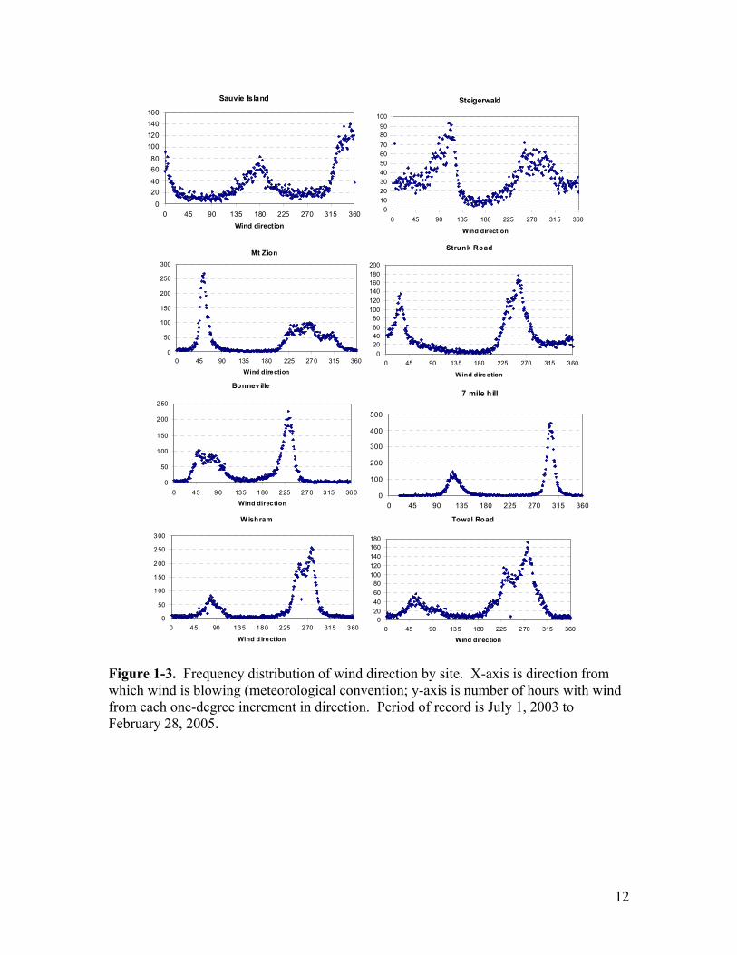
Figure 1-3. Frequency distribution of wind direction by site. X-axis is direction from which wind is blowing (meteorological convention; y-axis is number of hours with wind from each one-degree increment in direction. Period of record is July 1, 2003 to February 28, 2005..................................................................................... 12
Figure 1-4. Daily average upgorge wind speed by cluster for each monitoring site (miles per hour).......................................................................................................... 13
Figure 1-5. Frequency of occurrence of each cluster by month. ...................................... 14 Figure 1-6. Average bsp (Mm-1) at each nephelometer site for each cluster. Average is
over all hours for all days within each cluster. .......................................................... 15 Figure 3-1. Comparison between measured and reconstructed PM2.5 mass. .................... 21 Figure 3-2. Comparison between measured and reconstructed PM2.5 mass after
removing the three outliers. ....................................................................................... 22 Figure 3-3. PM2.5 chemical speciation based on IMPROVE-like samples....................... 22 Figure 3-4. PM2.5 chemical speciation (µg/m3) based on IMPROVE data (7/2003 -
12/2004) collected at COGO1 (Mt. Zion) and CORI1 (Wishram)............................ 24 Figure 3-5. Comparison of seasonally averaged IMPROVE and IAS data during: a)
summer, b) fall, and c) winter.................................................................................... 25 Figure 3-6. Comparison between DRUM and IAS filter measured: a) sulfur, b) silicon,
and c) calcium concentrations for PM2.5 at Bonneville. ............................................ 27 Figure 3-7. Comparison between DRUM and IMPROVE filter measured: a) sulfur, b)
silicon, and c) calcium concentrations for PM2.5 at Mt. Zion.................................... 28 Figure 3-8. Comparison between 24-hour averages of high time-resolved: a) SO4
2-, b) NO3
-, c) OC, d) EC, and e) TC and measurements and IMPROVE daily filter measurements at Mt. Zion. ........................................................................................ 30
Figure 3-9. Comparison between 24-hour averages of high time-resolved: a) SO42-, b)
NO3-, c) OC, d) EC, and e) TC measurements and IMPROVE daily filter
measurements at Wishram......................................................................................... 31 Figure 3-10. Comparison between 24-hour average of high time-resolved: a) SO4
-2, b) NO3
-, c) OC, d) EC, and e) TC measurements and daily IAS filter measurements at Bonneville. ............................................................................................................. 32
Figure 3-11. Average ratio of Optec nephelometer light scattering to Radiance Research nephelometer light scattering by integer-relative humidity value. ............ 34
Figure 3-12. Example time series comparison of Optec and Radiance Research light scattering at Mt. Zion................................................................................................. 34
Figure 3-13. Scatterplot of Optec light scattering versus Radiance Research light scattering adjusted by RH, Mt. Zion.......................................................................... 35
Figure 3-14. Scatterplot of Optec light scattering versus Radiance Research light scattering adjusted by RH, Wishram. ........................................................................ 35
6
Figure 3-15. Calculated wet light scattering coefficient of PM10 using IMPROVE aerosol data from Wishram versus daily average Optec nephelometer measured aerosol light scattering coefficient at Wishram. ........................................................ 38
Figure 3-16. Contribution of major chemical components to aerosol light extinction (light scattering + light absorption by LAC) coefficient at Wishram........................ 38
Figure 3-17. Calculated wet light scattering coefficient of PM10 using IMPROVE aerosol data from Mt. Zion versus daily average Optec nephelometer measured aerosol light extinction coefficient at Mt. Zion. ........................................................ 39
Figure 3-18. Contribution of major chemical components to aerosol light extinction (light scattering + light absorption by LAC) coefficient at Mt. Zion. ....................... 39
Figure 3-19. Calculated "dry" light scattering coefficient of PM10 using IMPROVE aerosol data from Wishram vs. daily average measured aerosol light extinction coefficient at Wishram............................................................................................... 41
Figure 3-20. Average contribution of major aerosol components to dry aerosol light extinction coefficient (light scattering + light absorption by LAC) at Wishram based on IMPROVE data from Wishram. ................................................................. 41
Figure 3-21. Calculated "dry" light scattering coefficient of PM10 using IMPROVE aerosol data from Mt. Zion versus daily average measured aerosol light extinction coefficient at Mt. Zion. .............................................................................................. 42
Figure 3-22. Average contribution of major aerosol components to dry aerosol light extinction coefficient (light scattering + light absorption by LAC) at Mt. Zion based on IMPROVE data from Mt. Zion................................................................... 42
Figure 3-23. Relationship between measured aerosol light scattering coefficient (bsp, Mm-1) and sum of light scattering due to OC, sulfate, and nitrate in Bonneville...... 43
Figure 3-24. Average contribution to aerosol light scattering at Bonneville................... 43 Figure 3-25. Relationship between measured aerosol light scattering coefficient (bsp,
Mm-1) and sum of light scattering due to OC, sulfate, and nitrate at Mt. Zion. ........ 44 Figure 3-26. Relationship between measured aerosol light scattering coefficient (bsp,
Mm-1) and sum of light scattering due to OC, sulfate, and nitrate at Wishram......... 45 Figure 3-27. Relationship between Optec measured aerosol light scattering coefficient
(bsp, Mm-1) and sum of light scattering due to OC, sulfate, and nitrate at Mt. Zion.. 46 Figure 3-28. Relationship between Optec measured aerosol light scattering coefficient
(bsp, Mm-1) and sum of light scattering due to OC, sulfate, and nitrate at Wishram. 46 Figure 3-29. Sunset Laboratory EC concentration (µg/m3) versus aethalometer-
derived EC (µg/m3) at Mt. Zion................................................................................. 47 Figure 3-30. Sunset Laboratory EC concentration (µg/m3) versus aethalometer-
derived EC (µg/m3) at Wishram. ............................................................................... 47 Figure 3-31. Monthly average ratio of positive to negative charge at Mt. Zion and
Wishram..................................................................................................................... 48 Figure 3-32. Estimated monthly average concentration of sulfate in the form of
ammonium bisulfate, ammonium sulfate, and unexplained sulfate for Wishram, 2004. For Figures 3-32 to 3-35, estimates are done individually by sample and then averaged over the number of samples per month. ............................................. 50
Figure 3-33. Estimated monthly average concentration of sulfate in the form of ammonium bisulfate, ammonium sulfate, and unexplained sulfate for Mt. Zion, 2004. .......................................................................................................................... 50

7
Figure 3-34. Estimated monthly average concentration of nitrate in the form of ammonium nitrate, sodium nitrate, potassium nitrate, and unexplained nitrate for Wishram, 2004........................................................................................................... 51
Figure 3-35. Estimated monthly average concentration of nitrate in the form of ammonium nitrate, sodium nitrate, potassium nitrate, and unexplained nitrate for Mt. Zion, 2004. .......................................................................................................... 51
Figure 4-1. Factor profiles (µg/µg) resolved from PM2.5 samples at Mt. Zion. ............. 57 Figure 4-2. Average contribution of each factor to PM2.5 mass at Mt. Zion. .................. 58 Figure 4-3. Time series of: a) paper mill, b) oil combustion, c) nitrate-rich secondary,
d) sulfate-rich secondary, e) mobile, f) dust, and g) biomass smoke source contributions at Mt. Zion. .......................................................................................... 59
Figure 4-4. Factor profiles (µg/µg) resolved from PM2.5 samples at Wishram. .............. 63 Figure 4-5. Average contribution of each factor to PM2.5 mass at Wishram................... 64 Figure 4-6. Time series of: a) secondary sulfate, b) smoke, c) mobile, d) dust, and e)
secondary nitrate source contributions at Wishram................................................... 65 Figure 4-7. Contribution of each source factor to organic mass, sulfate, nitrate, and
reconstructed light extinction at: a) Mt. Zion and b) Wishram. ................................ 68 Figure 4-8. Source profiles for Mt. Zion based on PMF modeling for 2004 only............ 76 Figure 4-9. Source profiles for Wishram based on PMF modeling for 2004 only. .......... 77 Figure 4-10. Daily average particle light scattering for the November 2004 episode.
Also shown in wind pattern type. .............................................................................. 78 Figure 4-11. Particle light scattering and high time-resolved sulfate, nitrate, and
organic carbon at: a) Bonneville and b) Mt. Zion for the November 2004 episode.. 79 Figure 4-12. Time series of high time-resolved nitrate at Mt. Zion and Bonneville for
the November 2004 episode. ..................................................................................... 80 Figure 4-13. Time series of bsp and upgorge wind component at Sevenmile Hill during
the November 2004 episode. ..................................................................................... 80 Figure 4-14. Time series of light scattering (Mm-1) for the February 2004 episode. ....... 82 Figure 4-15. Upgorge wind component for the February 2004 episode at selected sites. 83 Figure 4-16. Time series of light scattering, NO3, and SO4 at Bonneville during the
February 2004 episode............................................................................................... 83 Figure 4-17. Time series of light scattering, NO3, SO4, and OC at Wishram during the
February 2004 episode............................................................................................... 84 Figure 4-18. Time series of bsp at selected sites for the August 2004 episode. ................ 85 Figure 4-19. Pressure at The Dalles minus pressure at Portland International Airport
(mb) for the August 2004 episode. Values greater than zero suggest flow from west to east (upgorge)................................................................................................ 85
Figure 4-20. Bsp, reconstructed bsp, and estimated bsp due to sulfate, nitrate, and organic carbon during the August 2004 episode. ...................................................... 86
Figure 4-21. Organic carbon concentrations at IMPROVE sites in the Pacific Northwest on August 13, 2004. ................................................................................. 87
Figure 4-22. Sulfate concentrations at IMPROVE sites in the Pacific Northwest on August 16, 2004......................................................................................................... 88
Figure 4-23. Pressure at Portland International Airport minus pressure at The Dalles during the July 2004 episode. .................................................................................... 89

8
Figure 4-24. Time series of bsp (Mm-1) and sulfate, nitrate, and organic carbon concentrations (µg/m3) at Bonneville during the July 2004 episode......................... 89
Figure 4-25. Time series of bsp (Mm-1) and sulfate, nitrate, and organic carbon concentrations at Mt. Zion during the July 2004 episode.......................................... 90
Figure 4-26. Time series of light scattering (Mm-1) at Bonneville and Mt. Zion during the July 2004 episode................................................................................................. 90
Figure 4-27. Time series of organic carbon at Bonneville and Mt. Zion during the July 2004 episode. ............................................................................................................. 91
Figure 4-28. Time series of sulfate at Bonneville and Mt. Zion during the July 2004 episode. ...................................................................................................................... 91
Figure 4-29. Time series of DRUM 0.34-0.56 µm particulate sulfur and sodium concentrations for the July-August 2004 DRUM samples. ....................................... 92
Figure 4-30. Time series of measured and reconstructed scattering and scattering by major components at Bonneville during the July 2004 episode. Reconstructed light scattering is computed for sulfate, nitrate, and organic carbon compounds only. ........................................................................................................................... 93
Figure 4-31. Time series of measured and reconstructed scattering and scattering by major components at Mt. Zion during the July 2004 episode. Reconstructed light scattering is computed for sulfate, nitrate, and organic carbon compounds only...... 93
Figure 4-32. Organic carbon concentrations at IMPROVE sites in the Pacific northwest on July 29, 2004........................................................................................ 94
Figure 4-33. Sulfate concentrations at IMPROVE sites in the Pacific northwest on July 29, 2004. .................................................................................................................... 95
Figure 5-1. Diurnal pattern of particle light scattering in summer in the western Gorge. 96
9
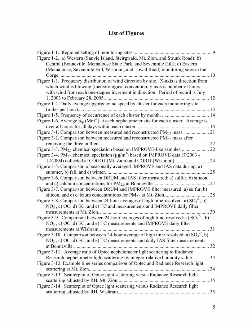
1. Introduction The Causes of Haze in the Gorge (CoHaGo) study is a data analysis effort intended to add to the understanding of the source areas and source types contributing significantly to haze in the Columbia River Gorge in the States of Washington and Oregon. The study is a follow-up to the Columbia River Gorge Haze Gradient Study (Green et. al, 2006). While the Haze Gradient Study used primarily nephelometer and surface meteorological data to understand spatial and temporal patterns in haze in the Gorge, CoHaGo makes use of additional aerosol chemical composition to enhance understanding of haze in the Gorge.
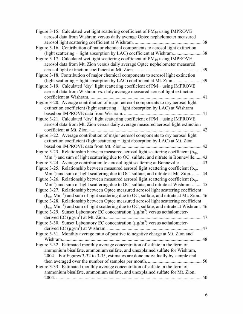
1.1 Summary of the Haze Gradient Study The field portion of the Columbia River Gorge Haze Gradient Study was conducted from July 2003 through February 2005. Nephelometers directly measured light scattering by particles (bsp), typically the largest component of haze, at nine locations from downriver from the Gorge (Sauvie Island) to upriver from the Gorge (Towal Road), including several sites in the Gorge. Monitoring site locations are shown in Figure 1-2 and 1-2. Meteorological measurements were taken at all sites except one (Memaloose).
Figure 1-1. Regional setting of monitoring sites.

10
(a)
Figure 1-2. a) Western (Sauvie Island, Steirgwald, Mt. Zion, and Strunk Road); b) Central (Bonneville, Memaloose State Park, and Sevenmile Hill); c) Eastern (Memaloose, Sevenmile Hill, Wishram, and Towal Road) monitoring sites in the Gorge.
(b)
11
(c)
Figure 1-2. Continued.
Because of the large number of days (>600) monitored, a statistical method (cluster analysis) was used to group days with similar wind patterns. Summaries of wind, pressure, particle light scattering (bsp), and light absorption were computed for each group of similar days (each cluster). Wind direction data showed that winds were channelled through the gorge with wind directions having a bi-modal distribution, upriver or downriver (Figure 1-3). Wind data were then classified as to their component upriver (basically west to east). Upriver was termed “upgorge”, downriver termed “downgorge”. Light scattering data were interpreted with respect to wind transport patterns to gain insight into likely source areas for each group of days.
Five clusters of similar days were identified:
1) light upgorge flow
2) moderate upgorge flow
3) strong upgorge flow
4) light downgorge flow (diurnal reversal at eastern sites)
5) winter downgorge flow (light at east end, strong at west end)
Daily averaged upgorge wind component for each cluster is shown in Figure 1-4.
12
Steigerwald
0102030405060708090
100
0 45 90 135 180 225 270 315 360
Wind direction
Sauvie Island
0
2040
6080
100120140160
0 45 90 135 180 225 270 315 360Wind direction
Mt Zion
0
50
100
150
200
250
300
0 45 90 135 180 225 270 315 360
Wind direction
Strunk Road
020406080
100120140160180200
0 45 90 135 180 225 270 315 360
Wind direction
7 mile hill
0
100
200
300
400
500
0 45 90 135 180 225 270 315 360
Wind directionTowal Road
020406080
100120140160180
0 45 90 135 180 225 270 315 360
Wind direction
W ishram
0
50
100
150
200
250
300
0 45 90 135 180 225 270 315 360
Wind d irect ion
Bonnev ille
0
50
100
150
200
250
0 45 90 135 180 225 270 315 360
Wind direction
Figure 1-3. Frequency distribution of wind direction by site. X-axis is direction from which wind is blowing (meteorological convention; y-axis is number of hours with wind from each one-degree increment in direction. Period of record is July 1, 2003 to February 28, 2005.

13
-15
-10
-5
0
5
10
15
20
Sau
vie
Stei
ger
Mt Z
ion
Stru
nk
Bonn
e
7 m
ile
Wis
h
Tow
al
daily
avr
eage
upg
orge
win
d (m
ph)
strong upgorge moderalte upgorge light upgorgelight downgorge winter downgorge
Figure 1-4. Daily average upgorge wind speed by cluster for each monitoring site (miles per hour).
The percentage frequency of occurrence of each cluster by month is shown tabularly in Table 1-1 and graphically in Figure 1-5.
Table 1-1. Percentage of days in each month assigned to each cluster type.
Cluster Jan Feb Mar Apr May Jun Jul Aug Sep Oct Nov Dec
1 15 9 19 27 13 13 9 19 18 24 19 25
2 6 5 13 20 29 33 29 40 35 27 12 13
3 6 14 35 20 48 37 56 35 28 18 17 6
4 10 21 16 27 10 17 5 5 18 22 28 19
5 63 51 16 7 0 0 0 0 0 9 24 38

14
0102030405060708090
100
Jan Feb Mar Apr May Jun Jul Aug Sep Oct Nov Dec
strong upgorge moderate upgorge light upgorgelight downgorge winter downgorge
Figure 1-5. Frequency of occurrence of each cluster by month.
Strong upgorge (3) was the predominant pattern in mid-summer; Winter downgorge (5) was the most frequent winter pattern and never occurred from May through September. Light upgorge (1) and light downgorge (4) were most frequent in fall and spring transition months; moderate upgorge (2) was most frequent in late summer to early fall.
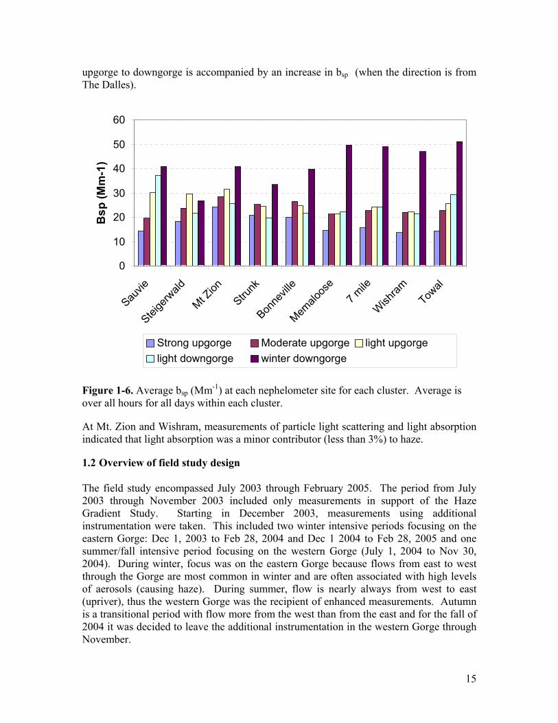
Winter downgorge (5) had the highest average bsp at all sites except Sauvie Island and Steigerwald (Figure 1-6). Highest bsp for winter downgorge was at the eastern sites, with a decrease with distance downgorge. Bsp increased again at Sauvie Island as the flow exited the Gorge and crossed the Portland/Vancouver area. This transport and bsp gradient pattern suggests that sources east of the Gorge cause much of the haze and that the Portland/Vancouver area contributes additional aerosol to the Sauvie Island site.
Light downgorge (4) had the highest b at Sauvie Island, suggesting impact from nearby sources such as the Portland/Vancouver area and/or downriver industry.
For days without precipitation, all the upgorge clusters (1-3) had highest bsp at Mt. Zion and a decreasing bsp with distance into the Gorge. Light upgorge (1) and moderate upgorge (2) showed diurnal patterns of increasing bsp progressing upgorge to the Bonneville site during the day. Bsp also increased across the Portland/Vancouver area for each cluster, suggesting the urban area as a significant contributor to aerosol in the Gorge for these clusters.
Light downgorge (4) and winter downgorge (5) showed an increase in bsp from Wishram to Sevenmile Hill and Memaloose, suggesting impact from The Dalles area. At Sevenmile Hill for light downgorge (4), the diurnal change in wind direction from
15
upgorge to downgorge is accompanied by an increase in bsp (when the direction is from The Dalles).
0
10
20
30
40
50
60
Sauvie
Steige
rwald
Mt Zion
Strunk
Bonne
ville
Memalo
ose
7 mile
Wish
ramTow
al
Bsp
(Mm
-1)
Strong upgorge Moderate upgorge light upgorgelight downgorge winter downgorge
Figure 1-6. Average bsp (Mm-1) at each nephelometer site for each cluster. Average is over all hours for all days within each cluster.
At Mt. Zion and Wishram, measurements of particle light scattering and light absorption indicated that light absorption was a minor contributor (less than 3%) to haze.
1.2 Overview of field study design
The field study encompassed July 2003 through February 2005. The period from July 2003 through November 2003 included only measurements in support of the Haze Gradient Study. Starting in December 2003, measurements using additional instrumentation were taken. This included two winter intensive periods focusing on the eastern Gorge: Dec 1, 2003 to Feb 28, 2004 and Dec 1 2004 to Feb 28, 2005 and one summer/fall intensive period focusing on the western Gorge (July 1, 2004 to Nov 30, 2004). During winter, focus was on the eastern Gorge because flows from east to west through the Gorge are most common in winter and are often associated with high levels of aerosols (causing haze). During summer, flow is nearly always from west to east (upriver), thus the western Gorge was the recipient of enhanced measurements. Autumn is a transitional period with flow more from the west than from the east and for the fall of 2004 it was decided to leave the additional instrumentation in the western Gorge through November.

16
Additional instruments provided continuous high-time resolved concentrations of sulfate, nitrate, organic carbon and elemental carbon. Used in conjunction with the light scattering (nephelometers) and surface meteorologic measurements this was anticipated to provide considerable insight into source type and areas contributing to haze in the Gorge. A detailed description of the monitoring program is given in Section 2.
17
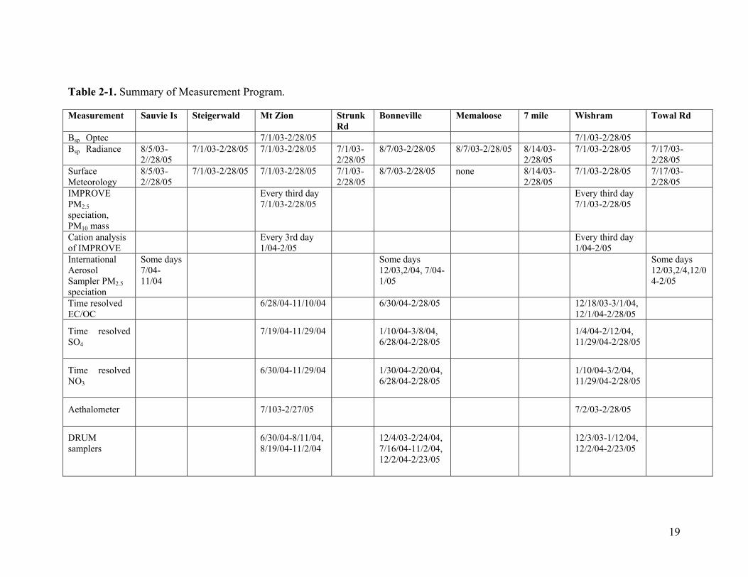
2. Field measurement program Table 2-1 is a summary of the field study measurements.
IMPROVE (Interagency Monitoring of Protected Visual Environments) samplers (http://vista.cira.colostate.edu/improve/) have been operating long-term at Wishram and Mt. Zion. They provide for chemical speciation of PM2.5 (particulate matter less than 2.5 microns in diameter) and mass of PM10 (particulate matter less than 10 microns in diameter)(Malm et al., 1994). The IMPROVE samplers operate one day in three so two-thirds of the days in the study period had no data from these samplers. From January 2004 – February 2005 additional ion analysis was done for the Wishram and Mt Zion IMPROVE samples. This included analysis of cations (NH4+, K+, Na+, Mg++, Ca++) as well as anions (in the standard analysis).
Light scattering was measured using Radiance Research M903 nephelometers at eight sites. The Radiance nephelometers are set to maintain relative humidity (RH) of not more than 50%; this is accomplished by heating the inlet air stream. This was done to allow for comparisons of scattering along the Gorge uncomplicated by different amounts of particle growth due to varying RH among sites. Optec NGN-2 nephelometers (Molenar, undated) were operated at Wishram and Mt. Zion; they have been operating long-term at these IMPROVE protocol sites. The Optec nephelometers are unheated and thus represent a more accurate estimate of light scattering, especially under higher RH conditions.
For some days corresponding to IMPROVE sampling days, PM2.5 filter samples using the “IMPROVE-like” International Aerosol Sampler (IAS) were collected at Sauvie Island (summer intensive), Bonneville (summer and winter intensives), and Towal Road (winter intensives) and chemically speciated. The IAS unit collected 24-hour time-integrated aerosol samples in the PM2.5 mode on three independent channels for analysis of mass, and elemental, ion, and elemental/organic carbon fraction. The IAS collected samples 1 day in 3 to match IMPROVE sampling dates during the Columbia River Gorge Study. Unlike the IMPROVE “module” which contains 3 unique PM2.5 samplers, the IAS uses the IMPROVE cyclone to effect a PM2.5 cutpoint and traps the particles on 3 independent filters for analysis. Thus, the flow rate (23 liters/minute) and cyclone, cassette and filter media are identical to the IMPROVE units, but 1/3 the flow (i.e. ~7.7 liters/minute) and consequently one-third as much sample is collected on each filter compared to the IMPROVE sampler.
A Sunset Laboratory carbon analyzer (Birch and Cary, 1996) was operated at Mt Zion during summer-fall 2004, at Bonneville from summer 2004-winter 2005, and at Wishram during winter 2003-2004 and winter 2004-2005. This instrument gave nearly continuous concentrations of organic and elemental carbon (OC/EC) for 2 hour periods (1 hour 45 minutes sampling followed by 15 minutes of analysis time each 2 hours). The analysis uses thermal optical transmittance to account for pyrolized carbon. This is in contrast to the thermal optical reflectance method used for the filter samples (from the IMPROVE and IAS samplers). Due to the use of transmittance and a different temperature program used, the method is expected to give lower elemental carbon than from the IMPROVE
18
and IAS samples but similar total (organic plus elemental) carbon (Chow et al., 2001, Chow et al., 2004).
Sulfate and nitrate were measured at the same locations and for approximately the same time periods as the OC/EC measurements. The instrumentation was Rupprecht & Patashnick series 8400S for sulfate and series 8400N for nitrate. Continuous data are available at 10 minute intervals.
As part of the haze gradient study, Aethalometers (Allen et al., 1999; Moosmuller et al., 1998) were operated at Wishram and Mt. Zion from July 2003- February 2005. Aethalometers give an estimate of elemental carbon by determining absorption due to particles deposited on a filter. Data is available for 5 minute average time periods, but is generally better when averaged over a longer time interval (e.g. one-hour).
Surface meteorology (wind speed and direction, temperature, and relative humidity) was measured at all nephelometer sites except Memaloose State Park.
Davis Rotating Drum Universal Monitors (DRUM) samplers (Raabe et al., 1988; Lundgren, 1967; Bench et al., 2002) were operated at Mt. Zion in the summer to fall 2004, at Bonneville from summer 2004 to winter 2004-2005 and at Wishram during winter 2003-2004 and winter 2004-2005. The DRUM sampler allows for analysis of chemical composition of collected particles in 3 hour time increments and 8 different sizes. The 8-Stage Rotating DRUM Impactor Sampler (8-RDI) is a cascade impactor. The sampler used operated at 16.7 liters per minute allowing it to couple to a 10 µm cutpoint (“PM10”) inlet (URG Corp.). The aerosol sample for each stage is deposited onto a rotating drum faced with a removable greased Mylar impaction surface. As the drum rotates a continuous aerosol sample is laid down along the direction of rotation with density varying along the length of the Mylar strip in proportion to the aerosol collected as the substrate rotates. Analysis using narrow beam techniques (s-XRF (Knochel,1990) and Proton Elastic scattering Analysis (PESA, Bench et al., 2002)) for elements and hydrogen, respectively, and Beta-ray attenuation for mass produces data with time resolution proportional to the ratio of drum surface speed divided by the beam width. Sampling allowed 42-day continuous record in 8 size bins (10-5, 5-2.5, 2.5-1.15, 1.15-0.75, 0.75-0.56, 0.56-0.34, 0.34-0.26, 0.26-0.09 micrometers aerodynamic diameter) analyzable in 3-hr time steps.
For the DRUM analysis, the accuracy is approximately 5% (set by the accuracy of the standards and correlation with those). Uncertainty reported in the database incorporates analytical uncertainty, flowrate uncertainty, etc.). The analytical precision is roughly 10% (comparing reruns).
19
Table 2-1. Summary of Measurement Program.
Measurement Sauvie Is Steigerwald Mt Zion Strunk Rd
Bonneville Memaloose 7 mile Wishram Towal Rd
Bsp Optec 7/1/03-2/28/05 7/1/03-2/28/05 Bsp Radiance 8/5/03-
2//28/05 7/1/03-2/28/05 7/1/03-2/28/05 7/1/03-
2/28/05 8/7/03-2/28/05 8/7/03-2/28/05 8/14/03-
2/28/05 7/1/03-2/28/05 7/17/03-
2/28/05 Surface Meteorology
8/5/03-2//28/05
7/1/03-2/28/05 7/1/03-2/28/05 7/1/03-2/28/05
8/7/03-2/28/05 none 8/14/03-2/28/05
7/1/03-2/28/05 7/17/03-2/28/05
IMPROVE PM2.5 speciation, PM10 mass
Every third day 7/1/03-2/28/05
Every third day 7/1/03-2/28/05
Cation analysis of IMPROVE
Every 3rd day 1/04-2/05
Every third day 1/04-2/05
International Aerosol Sampler PM2.5 speciation
Some days 7/04-11/04
Some days 12/03,2/04, 7/04-1/05
Some days 12/03,2/4,12/04-2/05
Time resolved EC/OC
6/28/04-11/10/04 6/30/04-2/28/05
12/18/03-3/1/04, 12/1/04-2/28/05
Time resolved SO4
7/19/04-11/29/04 1/10/04-3/8/04, 6/28/04-2/28/05
1/4/04-2/12/04, 11/29/04-2/28/05
Time resolved NO3
6/30/04-11/29/04 1/30/04-2/20/04, 6/28/04-2/28/05
1/10/04-3/2/04, 11/29/04-2/28/05
Aethalometer 7/103-2/27/05 7/2/03-2/28/05
DRUM samplers
6/30/04-8/11/04, 8/19/04-11/2/04
12/4/03-2/24/04, 7/16/04-11/2/04, 12/2/04-2/23/05
12/3/03-1/12/04, 12/2/04-2/23/05
20
3. Statistical Description of Data In this section summaries of the monitoring data are presented. In addition to summarizing measurements from each instrument, we compare measurements of the same compounds measured by different instruments at the same site (e.g. IMPROVE OC versus time-resolved OC by Sunset Laboratory instrument); and measured versus derived parameters (such as measured and reconstructed light scattering). These summaries and comparisons are done in order to better understand the quality of the data and the appropriate uses for each measurement.
Before proceeding with the data comparisons it is helpful to note that the only data used explicitly in source attribution analysis was the IMPROVE data at Wishram and Mt. Zion. Other data such as the IAS data, high-time resolved sulfate, nitrate, OC/EC, and nephelometer data were used qualitatively to help form conceptual models of the causes of haze in the gorge and to give additional information on spatial and temporal patterns. As will be seen in the comparisons that follow, some of the data was not as consistent as we hoped for and should be considered semi-quantitative. However, it is still useful, especially during for analysis of episodes of high-light scattering conditions. At the end of this section, we present a table that summarizes the authors opinions regarding quality of the data and appropriate uses.
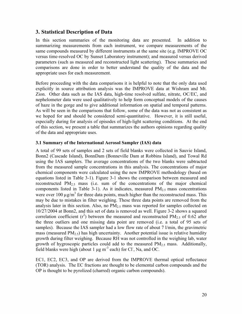
3.1 Summary of the International Aerosol Sampler (IAS) data A total of 99 sets of samples and 2 sets of field blanks were collected in Sauvie Island, Bonn2 (Cascade Island), BonnDam (Bonneville Dam at Robbins Island), and Towal Rd using the IAS samplers. The average concentrations of the two blanks were subtracted from the measured sample concentrations in this analysis. The concentrations of major chemical components were calculated using the new IMPROVE methodology (based on equations listed in Table 3-1). Figure 3-1 shows the comparison between measured and reconstructed PM2.5 mass (i.e. sum of the concentrations of the major chemical components listed in Table 3-1). As it indicates, measured PM2.5 mass concentrations were over 100 µg/m3 for three data points, much higher than the reconstructed mass. This may be due to mistakes in filter weighing. These three data points are removed from the analysis later in this section. Also, no PM2.5 mass was reported for samples collected on 10/27/2004 at Bonn2, and this set of data is removed as well. Figure 3-2 shows a squared correlation coefficient (r2) between the measured and reconstructed PM2.5 of 0.62 after the three outliers and one missing data point are removed (i.e. a total of 95 sets of samples). Because the IAS sampler had a low flow rate of about 7 l/min, the gravimetric mass (measured PM2.5) has high uncertainty. Another potential issue is relative humidity growth during filter weighing. Because RH was not controlled in the weighing lab, water growth of hygroscopic particles could add to the measured PM2.5 mass. Additionally, field blanks were high (about 1 µg m-3 each) for Cl-, Na, and OC.
EC1, EC2, EC3, and OP are derived from the IMPROVE thermal optical reflectance (TOR) analysis. The EC fractions are thought to be elemental carbon compounds and the OP is thought to be pyrolized (charred) organic carbon compounds).
21
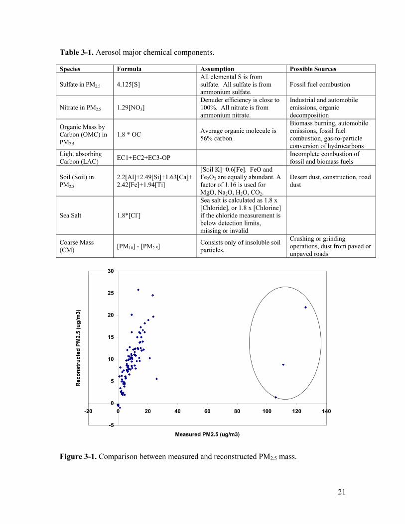
Table 3-1. Aerosol major chemical components.
Species Formula Assumption Possible Sources
Sulfate in PM2.5 4.125[S] All elemental S is from sulfate. All sulfate is from ammonium sulfate.
Fossil fuel combustion
Nitrate in PM2.5 1.29[NO3] Denuder efficiency is close to 100%. All nitrate is from ammonium nitrate.
Industrial and automobile emissions, organic decomposition
Organic Mass by Carbon (OMC) in PM2.5
1.8 * OC Average organic molecule is 56% carbon.
Biomass burning, automobile emissions, fossil fuel combustion, gas-to-particle conversion of hydrocarbons
Light absorbing Carbon (LAC) EC1+EC2+EC3-OP Incomplete combustion of
fossil and biomass fuels
Soil (Soil) in PM2.5
2.2[Al]+2.49[Si]+1.63[Ca]+2.42[Fe]+1.94[Ti]
[Soil K]=0.6[Fe]. FeO and Fe2O3 are equally abundant. A factor of 1.16 is used for MgO, Na2O, H2O, CO2.
Desert dust, construction, road dust
Sea Salt 1.8*[Cl-]
Sea salt is calculated as 1.8 x [Chloride], or 1.8 x [Chlorine] if the chloride measurement is below detection limits, missing or invalid
Coarse Mass (CM) [PM10] - [PM2.5]
Consists only of insoluble soil particles.
Crushing or grinding operations, dust from paved or unpaved roads
-5
0
5
10
15
20
25
30
-20 0 20 40 60 80 100 120 140
Measured PM2.5 (ug/m3)
Rec
onst
ruct
ed P
M2.
5 (u
g/m
3)
Figure 3-1. Comparison between measured and reconstructed PM2.5 mass.
22
y = 0.72x + 2.82R2 = 0.62
-5
0
5
10
15
20
25
30
-5 0 5 10 15 20 25 30
Measured PM2.5 (ug/m3)
Rec
onst
ruct
ed P
M2.
5 (u
g/m
3)
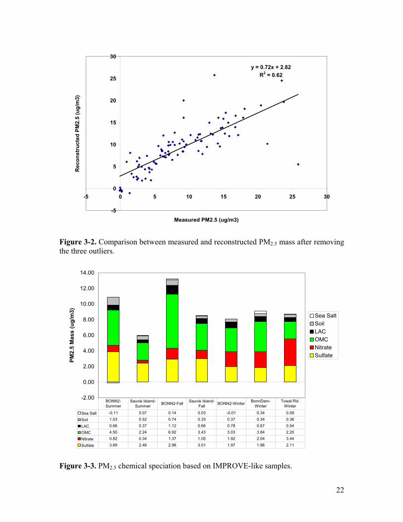
Figure 3-2. Comparison between measured and reconstructed PM2.5 mass after removing the three outliers.
-2.00
0.00
2.00
4.00
6.00
8.00
10.00
12.00
14.00
PM2.
5 M
ass
(ug/
m3)
Sea SaltSoilLACOMCNitrateSulfate
Sea Salt -0.11 0.07 0.14 0.03 -0.01 0.34 0.09
Soil 1.03 0.52 0.74 0.33 0.37 0.34 0.36
LAC 0.66 0.37 1.12 0.66 0.78 0.67 0.54
OMC 4.50 2.24 6.92 3.43 3.03 3.84 2.20
Nitrate 0.82 0.34 1.37 1.05 1.92 2.04 3.44
Sulfate 3.89 2.46 2.96 3.01 1.97 1.86 2.11
BONN2-Summer
Sauvie Island-Summer BONN2-Fall Sauvie Island-
Fall BONN2-Winter BonnDam-Winter
Towal Rd-Winter
Figure 3-3. PM2.5 chemical speciation based on IMPROVE-like samples.

23
Figure 3-3 summaries the aerosol chemical speciation data measured at Sauvie Island, Bonn2 (Cascade Island), BonnDam (Bonneville Dam at Robbins Island) and Towal Rd using the IAS samplers. Figure 3-3 shows that sulfate and organics are the major aerosol components at Bonneville and Sauvie Island during the summer. Sulfate contributes about 36% and 41% to PM2.5 mass in Bonneville and Sauvie Island during the summer, and OMC contributes 42% and 37%, respectively. During the fall, 52% and 40% of PM2.5 is organics in Bonneville and Sauvie Island, and sulfate contributes 22% and 35%, respectively. In the winter, OMC contributes 38% and 42% to PM2.5 mass at Bonn2 and BonnDam, and sulfate and nitrate each contributes about 20-25% at both sites. Nitrate is the largest contributor to PM2.5 at Towal road in winter, with a contribution of 39%. OMC and sulfate each contributes about 25% during winter at Towal road.
Bonneville had higher concentrations of sulfate, nitrate and OMC than Sauvie Island in summer and higher OMC in fall, although sulfate and nitrate levels were similar in fall. In winter, Wishram had higher nitrate than the Bonneville sites, while Bonneville had higher OMC and sulfate was about the same as at Wishram. It should be noted that the sea salt values have high uncertainty because of the large field blank values for chlorine.
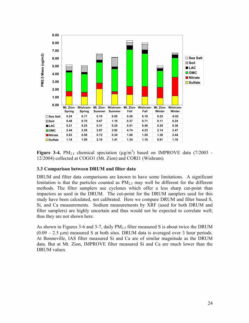
3.2 Comparison of IMPROVE and IAS aerosol data Figure 3-4 summarizes the seasonal average chemical speciation of PM2.5 based on IMPROVE aerosol data at Mt. Zion and Wishram. OMC is the largest contributor to PM2.5 at both sites during each season although nitrate is about equal to OMC in winter at Wishram. The figure also indicates that, in average, the aerosol loading and chemical speciation at Mt. Zion and Wishram are pretty similar, though sulfate concentration is slightly higher at Mt. Zion during the summer and nitrate is higher at Wishram during the winter.
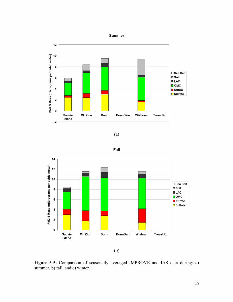
Figure 3-5 shows the comparison of seasonally averaged IMPROVE and IAS filter data during the time periods when IAS samples were collected. The sites are ordered from west to east in the figures. It is emphasized that the seasonal averages are not for the same set of days for each site listed so that direct comparisons are not presented here. The aerosol loading at Sauvie Island is generally lower than other sites in summer and fall. Sauvie Island did have some anomylously low concentration days in November 2004 that calls in to doubt the lower average concentrations there. In general, there is relatively more organic mass on the west side of gorge during the summer and fall, and more nitrate on the east side of the gorge during the winter. Calculated PM2.5 light scattering versus measured light scattering at Bonneville showed them to be highly correlated (r2=0.86) while low correlations existed for Sauvie Island and Towal Road suggesting measurement problems at these two IAS sampler sites.
24
0.00
1.00
2.00
3.00
4.00
5.00
6.00
7.00
8.00
9.00
PM2.
5 M
ass
(ug/
m3)
Sea SaltSoilLACOMCNitrateSulfate
Sea Salt 0.24 0.17 0.10 0.05 0.26 0.18 0.22 -0.02Soil 0.48 0.70 0.67 1.19 0.37 0.71 0.11 0.24LAC 0.21 0.25 0.31 0.25 0.51 0.46 0.29 0.38OMC 2.44 2.29 2.67 2.92 4.74 4.23 2.14 2.47Nitrate 0.63 0.58 0.72 0.34 1.08 1.29 1.36 2.44Sulfate 1.14 1.09 2.10 1.41 1.34 1.10 0.91 1.16
Mt. Zion-Spring
Wishram-Spring
Mt. Zion-Summer
Wishram-Summer
Mt. Zion-Fall
Wishram-Fall
Mt. Zion-Winter
Wishram-Winter
Figure 3-4. PM2.5 chemical speciation (µg/m3) based on IMPROVE data (7/2003 - 12/2004) collected at COGO1 (Mt. Zion) and CORI1 (Wishram).
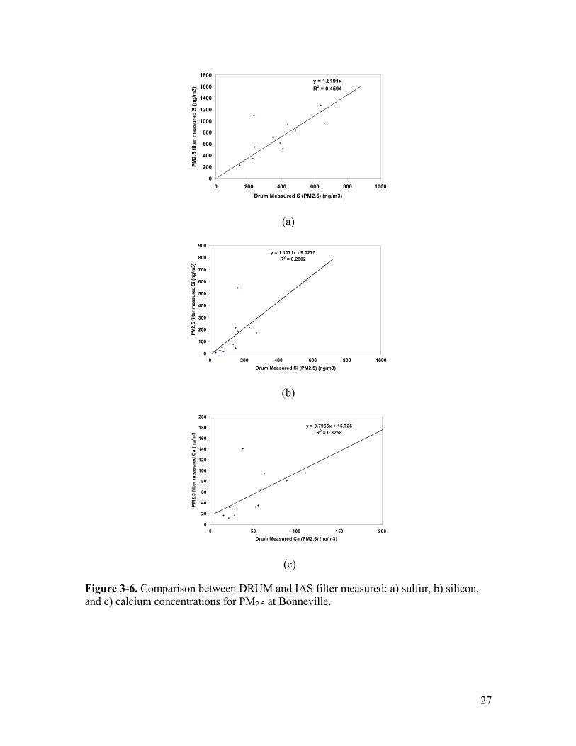
3.3 Comparison between DRUM and filter data DRUM and filter data comparisons are known to have some limitations. A significant limitation is that the particles counted as PM2.5 may well be different for the different methods. The filter samplers use cyclones which offer a less sharp cut-point than impactors as used in the DRUM. The cut-point for the DRUM samplers used for this study have been calculated, not calibrated. Here we compare DRUM and filter based S, Si, and Ca measurements. Sodium measurements by XRF (used for both DRUM and filter samplers) are highly uncertain and thus would not be expected to correlate well; thus they are not shown here.
As shown in Figures 3-6 and 3-7, daily PM2.5 filter measured S is about twice the DRUM (0.09 – 2.5 µm) measured S at both sites. DRUM data is averaged over 3 hour periods. At Bonneville, IAS filter measured Si and Ca are of similar magnitude as the DRUM data. But at Mt. Zion, IMPROVE filter measured Si and Ca are much lower than the DRUM values.
25
Summer
-2
0
2
4
6
8
10
12
SauvieIsland
Mt. Zion Bonn BonnDam Wishram Towal Rd
PM2.
5 M
ass
(mic
rogr
ams
per c
ubic
met
er)
Sea SaltSoilLACOMCNitrateSulfate
(a)
Fall
0
2
4
6
8
10
12
14
SauvieIsland
Mt. Zion Bonn BonnDam Wishram Towal Rd
PM2.
5 M
ass
(mic
rogr
ams
per c
ubic
met
er)
Sea SaltSoilLACOMCNitrateSulfate
(b)
Figure 3-5. Comparison of seasonally averaged IMPROVE and IAS data during: a) summer, b) fall, and c) winter.

26
Winter
-2
0
2
4
6
8
10
12
SauvieIsland
Mt. Zion Bonn BonnDam Wishram Towal Rd
PM2.
5 M
ass
(mic
rogr
ams
per c
ubic
met
er)
Sea SaltSoilLACOMCNitrateSulfate
(c)
Figure 3-5. Continued.
27
y = 1.8191xR2 = 0.4594
0
200
400
600
800
1000
1200
1400
1600
1800
0 200 400 600 800 1000
Drum Measured S (PM2.5) (ng/m3) PM
2.5
filte
r mea
sure
d S
(ng/
m3)
(a)
y = 1.1071x - 9.0275R2 = 0.2802
0
100
200
300
400
500
600
700
800
900
0 200 400 600 800 1000Drum Measured Si (PM2.5) (ng/m3)
PM2.
5 fil
ter m
easu
red
Si (n
g/m
3)
(b)
y = 0.7965x + 15.726R2 = 0.3258
0
20
40
60
80
100
120
140
160
180
200
0 50 100 150 200Drum Measured Ca (PM2.5) (ng/m3)
PM
2.5
filte
r mea
sure
d C
a (n
g/m
3
(c)
Figure 3-6. Comparison between DRUM and IAS filter measured: a) sulfur, b) silicon, and c) calcium concentrations for PM2.5 at Bonneville.

28
y = 2.6159x + 243.97R2 = 0.7455
0
500
1000
1500
2000
2500
3000
3500
0 200 400 600 800 1000Drum Measured S (PM2.5) (ng/m3)
PM2.
5 fil
ter m
easu
red
S (n
g/m
3)
(a)
y = 0.3431x + 41.154R2 = 0.435
0
50
100
150
200
250
300
350
400
450
500
0 200 400 600 800 1000Drum Measured Si (PM2.5) (ng/m3)
PM2.
5 fil
ter m
easu
red
Si (n
g/m
3)
(b)
y = 0.3414x + 15.326R2 = 0.3198
0
20
40
60
80
100
120
0 50 100 150 200Drum Measured Ca (PM2.5) (ng/m3)
PM2.
5 fil
ter m
easu
red
Ca
(ng/
m3)
(c)
Figure 3-7. Comparison between DRUM and IMPROVE filter measured: a) sulfur, b) silicon, and c) calcium concentrations for PM2.5 at Mt. Zion.
29
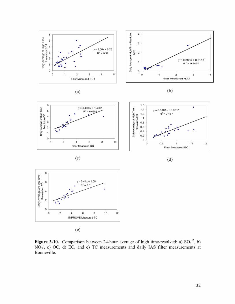
3.4 Comparisons between filter and high time resolved data High time resolved measurements of SO4, NO3, OC, EC, and total carbon (OC+EC) are compared to the 24-hour averaged IMPROVE measurements at Wishram and Mt. Zion and to the 24-hour averaged IAS measurements at Bonneville (Figures 3-8 to 3-10).
The time-resolved sulfate tended to be higher than the 24-hour filter sulfate at all sites. There was poor correlation at Wishram and Bonneville, but better correlation (r2=0.61) at Mt Zion. At Mt. Zion the time-resolved sulfate was about 50% higher than the IMPROVE sulfate.
Nitrate from the time-resolved and filter measurements tended to be of similar overall magnitude; the squared correlation coefficients ranged from r2=0.38 at Wishram to r2=0.85 at Bonneville.
OC concentrations measured by the time-resolved and filter methods were comparable. R2 ranged from 0.62 at Bonneville to 0.72 at Wishram.
For EC, the time resolved measurements gave about ½ the concentration of the filter based measurements at Mt. Zion and Bonneville and about three-eighths at Wishram. This is expected to result from both the different temperature programs applied to the Sunset Carbon analyzer compared to the IMPROVE temperature program and the use of transmittance rather than reflectance for determining the split between OC and EC (Chow et al., 2004). The correlations ranged from r2=0.46 at Bonneville to r2=0.62 at Wishram. For total carbon, at Mt. Zion and Wishram the Sunset analyzer total carbon is about two-thirds the IMPROVE filter carbon. The reason for this is not known. The Sunset analyzer has an organic gas denuder designed to remove organic gases that may absorb onto the sample and cause a positive artifact. The IMPROVE sampler does not have an organic gas denuder; there are considered to be positive artifacts from condensation of organic gases onto the filter and negative artifacts from desorption of particulate organics from the filter. For the Sunset analyzer, desorption of organic particulate is of less concern than for the IMPROVE samples because the analysis is performed every two hours in the field, presumably limiting the loss or organic particulate. On the other hand, perhaps the organic gas denuder removed some organic particulate matter. Consequently, because of the sampling methodologies, the Sunset analyzer may be expected have a lower total carbon concentration than the IMPROVE samplers.
At Bonneville, except for two outliers, the Sunset analyzer has similar total carbon concentrations as the IAS sampler. The outliers contribute substantially to a lowered r2, low slope, and high intercept.

30
y = 1.64x + 0.30R2 = 0.82
0
1
2
3
4
5
6
0 0.5 1 1.5 2 2.5 3IMPROVE Measured SO4
Dai
ly A
vera
ge o
f Hig
h Ti
me
Res
olut
ion
SO
4
(a)
y = 0.82x - 0.12R2 = 0.95
0
1
2
3
4
5
6
7
0 2 4 6 8
IMPROVE Measured NO3
Dai
ly A
vera
ge o
f Hig
h Ti
me
Res
olut
ion
NO
3
(b)
y = 0.74x + 0.44R2 = 0.91
0
12
3
4
56
7
89
0 2 4 6 8 10 12IMPROVE Measured OC
Dai
ly A
vera
ge o
f Hig
h Ti
me
Res
olut
ion
OC
(c)
y = 0.53x + 0.05R2 = 0.61
0
0.2
0.4
0.6
0.8
1
0 0.5 1 1.5
IMPROVE Measured EC
Dai
ly A
vera
ge o
f Hig
h Ti
me
Res
olut
ion
EC
(d)
y = 0.66x + 0.62R2 = 0.76
0
2
4
6
8
0 2 4 6 8 10
IMPROVE Measured TC
Dai
ly A
vera
ge o
f Hig
h Ti
me
Res
olut
ion
TC
(e)
Figure 3-8. Comparison between 24-hour averages of high time-resolved: a) SO42-, b)
NO3-, c) OC, d) EC, and e) TC and measurements and IMPROVE daily filter
measurements at Mt. Zion.

31
y = 0.789x + 0.6212R2 = 0.2149
00.5
11.5
2
2.53
3.54
0 1 2 3 4
IMPROVE Measured SO4
Dai
ly A
vera
ge o
f Hig
h Ti
me
Res
olut
ion
SO4
(a)
y = 0.4215x + 0.2232R2 = 0.3801
-1
0
1
2
3
4
5
6
0 2 4 6 8 10
IMPROVE Measured NO3
Dai
ly A
vera
ge o
f Hig
h Ti
me
Res
olut
ion
NO
3
(b)
y = 0.7085x + 0.6109R2 = 0.7195
0
0.5
1
1.5
2
2.5
3
3.5
4
0 1 2 3 4
IMPROVE Measured OC
Dai
ly A
vera
ge o
f Hig
h Ti
me
Res
olut
ion
OC
(c)
y = 0.3667x + 0.061R2 = 0.6232
0
0.1
0.2
0.3
0.4
0.5
0.6
0 0.2 0.4 0.6 0.8 1 1.2IMPROVE Measured EC
Dai
ly A
vera
ge o
f Hig
h Ti
me
Res
olut
ion
EC
(d)
y = 0.66x + 0.62R2 = 0.76
0
2
4
6
8
0 2 4 6 8 10
IMPROVE Measured TC
Dai
ly A
vera
ge o
f Hig
h Ti
me
Res
olut
ion
TC
(e)
Figure 3-9. Comparison between 24-hour averages of high time-resolved: a) SO42-, b)
NO3-, c) OC, d) EC, and e) TC measurements and IMPROVE daily filter measurements
at Wishram.
32
y = 1.06x + 0.76R2 = 0.37
0
1
2
3
4
5
6
0 1 2 3 4 5
Filter Measured SO4
Dai
ly A
vera
ge o
f Hig
h Ti
me
Res
olut
ion
SO
4
(a)
y = 0.883x + 0.0118R2 = 0.8497
0
1
2
3
4
0 1 2 3 4
Filter Measured NO3
Dai
ly A
vera
ge o
f Hig
h Ti
me
Res
olut
ion
NO
3
(b)
y = 0.4607x + 1.4307R2 = 0.6202
0
1
2
3
4
5
6
0 2 4 6 8 10Filter Measured OC
Dai
ly A
vera
ge o
f Hig
h Ti
me
Res
olut
ion
OC
(c)
y = 0.5181x + 0.0311R2 = 0.457
0
0.2
0.4
0.6
0.8
1
1.2
1.4
1.6
0 0.5 1 1.5 2Filter Measured EC
Dai
ly A
vera
ge o
f Hig
h Ti
me
Res
olut
ion
EC
(d)
y = 0.44x + 1.58R2 = 0.61
0
2
4
6
8
0 2 4 6 8 10 12
IMPROVE Measured TC
Dai
ly A
vera
ge o
f Hig
h Ti
me
Res
olut
ion
TC
(e)
Figure 3-10. Comparison between 24-hour average of high time-resolved: a) SO4-2, b)
NO3-, c) OC, d) EC, and e) TC measurements and daily IAS filter measurements at
Bonneville.
33
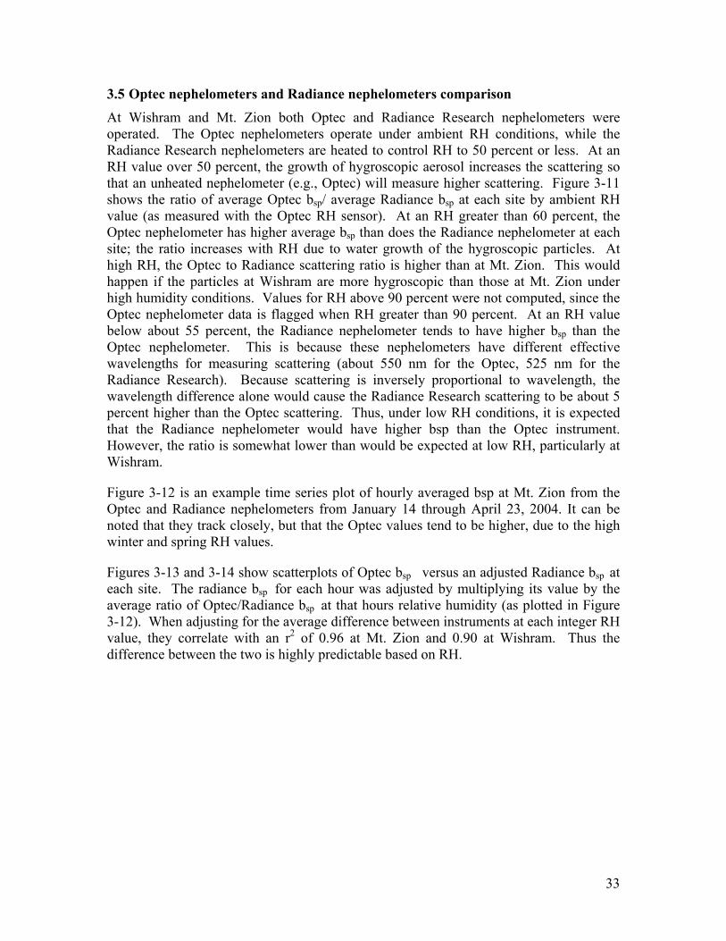
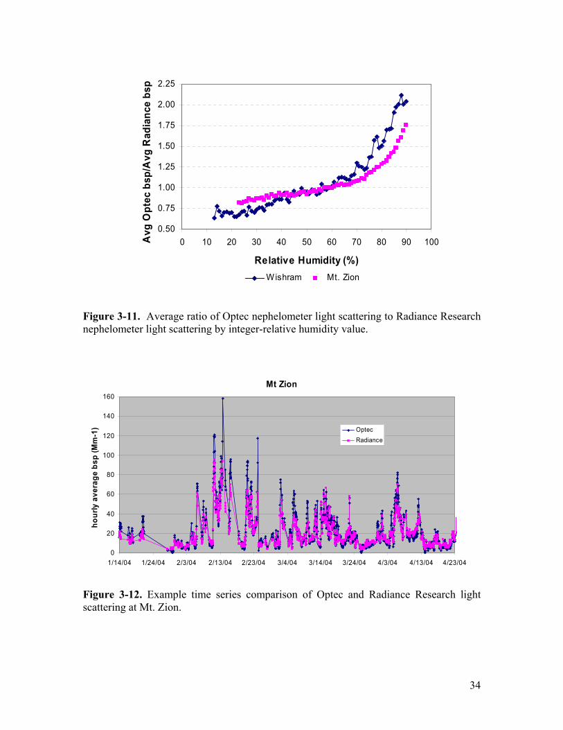
3.5 Optec nephelometers and Radiance nephelometers comparison At Wishram and Mt. Zion both Optec and Radiance Research nephelometers were operated. The Optec nephelometers operate under ambient RH conditions, while the Radiance Research nephelometers are heated to control RH to 50 percent or less. At an RH value over 50 percent, the growth of hygroscopic aerosol increases the scattering so that an unheated nephelometer (e.g., Optec) will measure higher scattering. Figure 3-11 shows the ratio of average Optec bsp/ average Radiance bsp at each site by ambient RH value (as measured with the Optec RH sensor). At an RH greater than 60 percent, the Optec nephelometer has higher average bsp than does the Radiance nephelometer at each site; the ratio increases with RH due to water growth of the hygroscopic particles. At high RH, the Optec to Radiance scattering ratio is higher than at Mt. Zion. This would happen if the particles at Wishram are more hygroscopic than those at Mt. Zion under high humidity conditions. Values for RH above 90 percent were not computed, since the Optec nephelometer data is flagged when RH greater than 90 percent. At an RH value below about 55 percent, the Radiance nephelometer tends to have higher bsp than the Optec nephelometer. This is because these nephelometers have different effective wavelengths for measuring scattering (about 550 nm for the Optec, 525 nm for the Radiance Research). Because scattering is inversely proportional to wavelength, the wavelength difference alone would cause the Radiance Research scattering to be about 5 percent higher than the Optec scattering. Thus, under low RH conditions, it is expected that the Radiance nephelometer would have higher bsp than the Optec instrument. However, the ratio is somewhat lower than would be expected at low RH, particularly at Wishram.
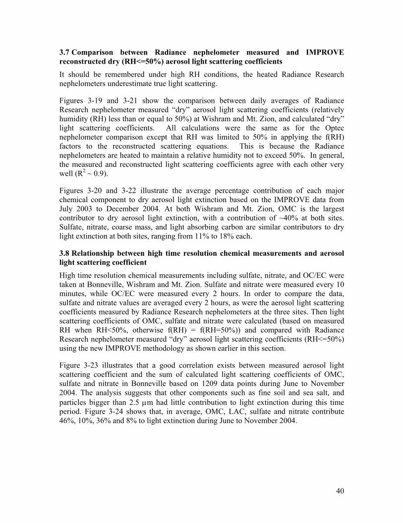
Figure 3-12 is an example time series plot of hourly averaged bsp at Mt. Zion from the Optec and Radiance nephelometers from January 14 through April 23, 2004. It can be noted that they track closely, but that the Optec values tend to be higher, due to the high winter and spring RH values.
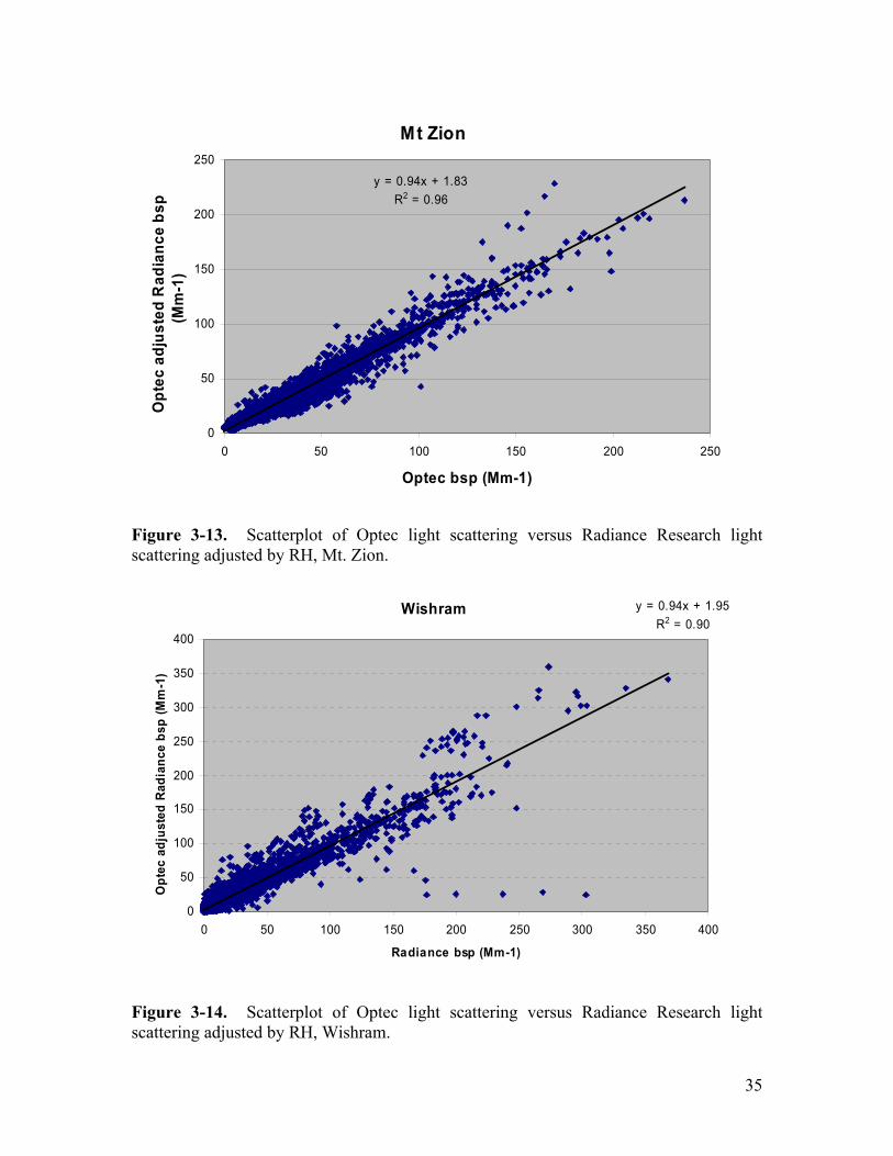
Figures 3-13 and 3-14 show scatterplots of Optec bsp versus an adjusted Radiance bsp at each site. The radiance bsp for each hour was adjusted by multiplying its value by the average ratio of Optec/Radiance bsp at that hours relative humidity (as plotted in Figure 3-12). When adjusting for the average difference between instruments at each integer RH value, they correlate with an r2 of 0.96 at Mt. Zion and 0.90 at Wishram. Thus the difference between the two is highly predictable based on RH.
34
0.50
0.75
1.00
1.25
1.50
1.75
2.00
2.25
0 10 20 30 40 50 60 70 80 90 100
Relative Humidity (%)
Avg
Opt
ec b
sp/A
vg R
adia
nce
bsp
Wishram Mt. Zion
Figure 3-11. Average ratio of Optec nephelometer light scattering to Radiance Research nephelometer light scattering by integer-relative humidity value.
Mt Zion
0
20
40
60
80
100
120
140
160
1/14/04 1/24/04 2/3/04 2/13/04 2/23/04 3/4/04 3/14/04 3/24/04 4/3/04 4/13/04 4/23/04
hour
ly a
vera
ge b
sp (M
m-1
) OptecRadiance
Figure 3-12. Example time series comparison of Optec and Radiance Research light scattering at Mt. Zion.
35
Mt Zion
y = 0.94x + 1.83R2 = 0.96
0
50
100
150
200
250
0 50 100 150 200 250
Optec bsp (Mm-1)
Opt
ec a
djus
ted
Rad
ianc
e bs
p (M
m-1
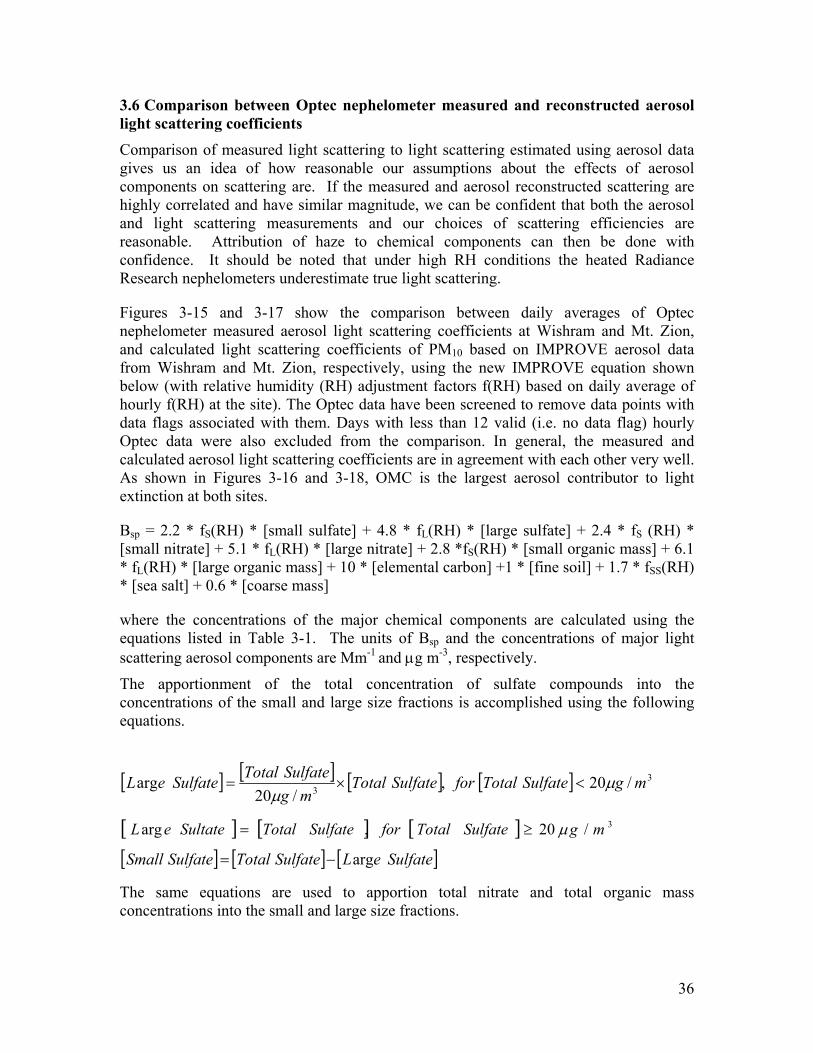
)
Figure 3-13. Scatterplot of Optec light scattering versus Radiance Research light scattering adjusted by RH, Mt. Zion.
Wishram y = 0.94x + 1.95R2 = 0.90
0
50
100
150
200
250
300
350
400
0 50 100 150 200 250 300 350 400
Radiance bsp (Mm-1)
Opt
ec a
djus
ted
Rad
ianc
e bs
p (M
m-1
)
Figure 3-14. Scatterplot of Optec light scattering versus Radiance Research light scattering adjusted by RH, Wishram.
36
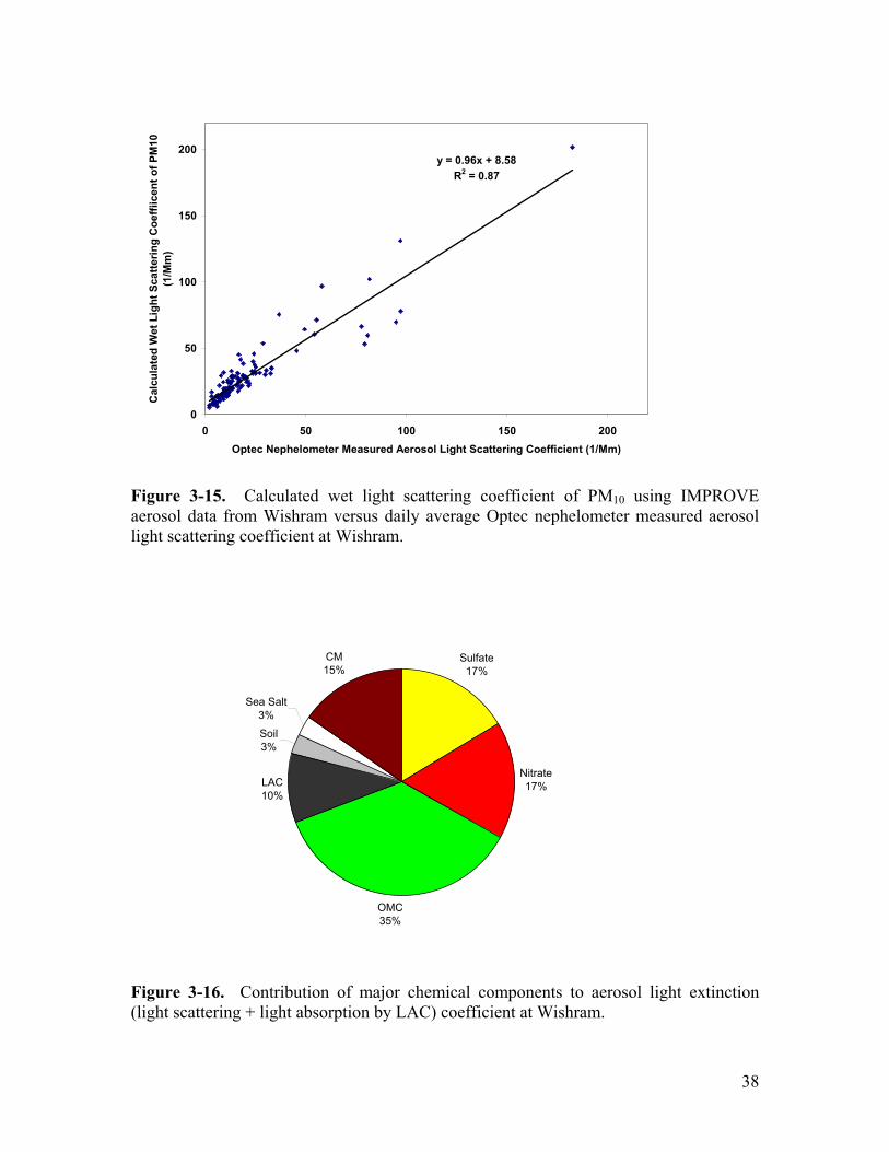
3.6 Comparison between Optec nephelometer measured and reconstructed aerosol light scattering coefficients Comparison of measured light scattering to light scattering estimated using aerosol data gives us an idea of how reasonable our assumptions about the effects of aerosol components on scattering are. If the measured and aerosol reconstructed scattering are highly correlated and have similar magnitude, we can be confident that both the aerosol and light scattering measurements and our choices of scattering efficiencies are reasonable. Attribution of haze to chemical components can then be done with confidence. It should be noted that under high RH conditions the heated Radiance Research nephelometers underestimate true light scattering.
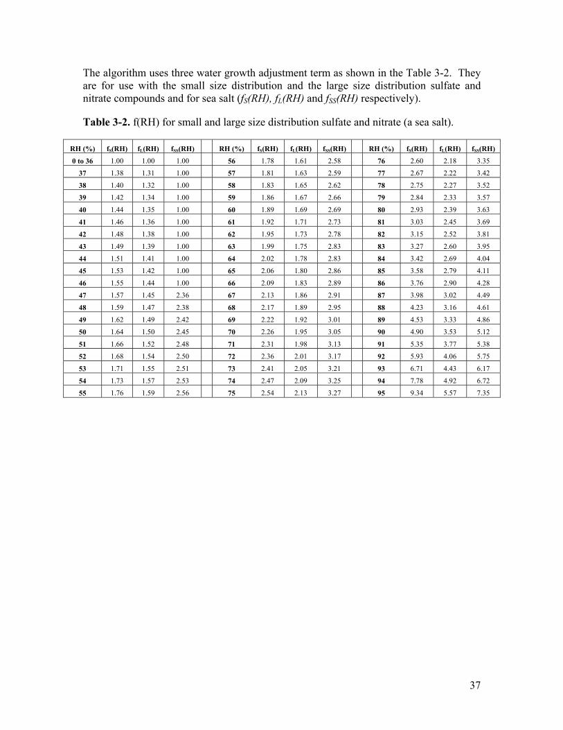
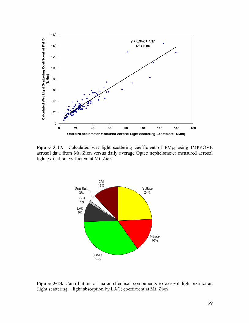
Figures 3-15 and 3-17 show the comparison between daily averages of Optec nephelometer measured aerosol light scattering coefficients at Wishram and Mt. Zion, and calculated light scattering coefficients of PM10 based on IMPROVE aerosol data from Wishram and Mt. Zion, respectively, using the new IMPROVE equation shown below (with relative humidity (RH) adjustment factors f(RH) based on daily average of hourly f(RH) at the site). The Optec data have been screened to remove data points with data flags associated with them. Days with less than 12 valid (i.e. no data flag) hourly Optec data were also excluded from the comparison. In general, the measured and calculated aerosol light scattering coefficients are in agreement with each other very well. As shown in Figures 3-16 and 3-18, OMC is the largest aerosol contributor to light extinction at both sites.
Bsp = 2.2 * fS(RH) * [small sulfate] + 4.8 * fL(RH) * [large sulfate] + 2.4 * fS (RH) * [small nitrate] + 5.1 * fL(RH) * [large nitrate] + 2.8 *fS(RH) * [small organic mass] + 6.1 * fL(RH) * [large organic mass] + 10 * [elemental carbon] +1 * [fine soil] + 1.7 * fSS(RH) * [sea salt] + 0.6 * [coarse mass]
where the concentrations of the major chemical components are calculated using the equations listed in Table 3-1. The units of Bsp and the concentrations of major light scattering aerosol components are Mm-1 and µg m-3, respectively.
The apportionment of the total concentration of sulfate compounds into the concentrations of the small and large size fractions is accomplished using the following equations.
The same equations are used to apportion total nitrate and total organic mass concentrations into the small and large size fractions.
[ ] [ ] [ ] 3/20,rga mgSulfateTotalforSulfateTotalSultateeL µ≥=
[ ] [ ] [ ] [ ] 33 /20,
/20arg mgSulfateTotalforSulfateTotal
mgSulfateTotalSulfateeL µ
µ<×=
[ ] [ ] [ ]SulfateeLSulfateTotalSulfateSmall arg−=
37
The algorithm uses three water growth adjustment term as shown in the Table 3-2. They are for use with the small size distribution and the large size distribution sulfate and nitrate compounds and for sea salt (fS(RH), fL(RH) and fSS(RH) respectively).
Table 3-2. f(RH) for small and large size distribution sulfate and nitrate (a sea salt).
RH (%) fS(RH) fL(RH) fSS(RH) RH (%) fS(RH) fL(RH) fSS(RH) RH (%) fS(RH) fL(RH) fSS(RH)
0 to 36 1.00 1.00 1.00 56 1.78 1.61 2.58 76 2.60 2.18 3.35
37 1.38 1.31 1.00 57 1.81 1.63 2.59 77 2.67 2.22 3.42
38 1.40 1.32 1.00 58 1.83 1.65 2.62 78 2.75 2.27 3.52
39 1.42 1.34 1.00 59 1.86 1.67 2.66 79 2.84 2.33 3.57
40 1.44 1.35 1.00 60 1.89 1.69 2.69 80 2.93 2.39 3.63
41 1.46 1.36 1.00 61 1.92 1.71 2.73 81 3.03 2.45 3.69
42 1.48 1.38 1.00 62 1.95 1.73 2.78 82 3.15 2.52 3.81
43 1.49 1.39 1.00 63 1.99 1.75 2.83 83 3.27 2.60 3.95
44 1.51 1.41 1.00 64 2.02 1.78 2.83 84 3.42 2.69 4.04
45 1.53 1.42 1.00 65 2.06 1.80 2.86 85 3.58 2.79 4.11
46 1.55 1.44 1.00 66 2.09 1.83 2.89 86 3.76 2.90 4.28
47 1.57 1.45 2.36 67 2.13 1.86 2.91 87 3.98 3.02 4.49
48 1.59 1.47 2.38 68 2.17 1.89 2.95 88 4.23 3.16 4.61
49 1.62 1.49 2.42 69 2.22 1.92 3.01 89 4.53 3.33 4.86
50 1.64 1.50 2.45 70 2.26 1.95 3.05 90 4.90 3.53 5.12
51 1.66 1.52 2.48 71 2.31 1.98 3.13 91 5.35 3.77 5.38
52 1.68 1.54 2.50 72 2.36 2.01 3.17 92 5.93 4.06 5.75
53 1.71 1.55 2.51 73 2.41 2.05 3.21 93 6.71 4.43 6.17
54 1.73 1.57 2.53 74 2.47 2.09 3.25 94 7.78 4.92 6.72
55 1.76 1.59 2.56 75 2.54 2.13 3.27 95 9.34 5.57 7.35
38
y = 0.96x + 8.58R2 = 0.87
0
50
100
150
200
0 50 100 150 200Optec Nephelometer Measured Aerosol Light Scattering Coefficient (1/Mm)
Cal
cula
ted
Wet
Lig
ht S
catte
ring
Coe
ffiic
ent o
f PM
10
(1/M
m)
Figure 3-15. Calculated wet light scattering coefficient of PM10 using IMPROVE aerosol data from Wishram versus daily average Optec nephelometer measured aerosol light scattering coefficient at Wishram.
Sulfate17%
Nitrate17%
OMC35%
LAC10%
Soil3%
Sea Salt3%
CM15%
Figure 3-16. Contribution of major chemical components to aerosol light extinction (light scattering + light absorption by LAC) coefficient at Wishram.
39
y = 0.94x + 7.17R2 = 0.88
0
20
40
60
80
100
120
140
160
0 20 40 60 80 100 120 140 160Optec Nephelometer Measured Aerosol Light Scattering Coefficient (1/Mm)
Cal
cula
ted
Wet
Lig
ht S
catte
ring
Coe
ffiic
ent o
f PM
10
(1/M
m)
Figure 3-17. Calculated wet light scattering coefficient of PM10 using IMPROVE aerosol data from Mt. Zion versus daily average Optec nephelometer measured aerosol light extinction coefficient at Mt. Zion.
Sulfate24%
Nitrate16%
OMC35%
LAC9%
Soil1%
Sea Salt3%
CM12%
Figure 3-18. Contribution of major chemical components to aerosol light extinction (light scattering + light absorption by LAC) coefficient at Mt. Zion.
40
3.7 Comparison between Radiance nephelometer measured and IMPROVE reconstructed dry (RH<=50%) aerosol light scattering coefficients It should be remembered under high RH conditions, the heated Radiance Research nephelometers underestimate true light scattering.
Figures 3-19 and 3-21 show the comparison between daily averages of Radiance Research nephelometer measured “dry” aerosol light scattering coefficients (relatively humidity (RH) less than or equal to 50%) at Wishram and Mt. Zion, and calculated “dry” light scattering coefficients. All calculations were the same as for the Optec nephelometer comparison except that RH was limited to 50% in applying the f(RH) factors to the reconstructed scattering equations. This is because the Radiance nephelometers are heated to maintain a relative humidity not to exceed 50%. In general, the measured and reconstructed light scattering coefficients agree with each other very well (R2 ~ 0.9).
Figures 3-20 and 3-22 illustrate the average percentage contribution of each major chemical component to dry aerosol light extinction based on the IMPROVE data from July 2003 to December 2004. At both Wishram and Mt. Zion, OMC is the largest contributor to dry aerosol light extinction, with a contribution of ~40% at both sites. Sulfate, nitrate, coarse mass, and light absorbing carbon are similar contributors to dry light extinction at both sites, ranging from 11% to 18% each.
3.8 Relationship between high time resolution chemical measurements and aerosol light scattering coefficient High time resolution chemical measurements including sulfate, nitrate, and OC/EC were taken at Bonneville, Wishram and Mt. Zion. Sulfate and nitrate were measured every 10 minutes, while OC/EC were measured every 2 hours. In order to compare the data, sulfate and nitrate values are averaged every 2 hours, as were the aerosol light scattering coefficients measured by Radiance Research nephelometers at the three sites. Then light scattering coefficients of OMC, sulfate and nitrate were calculated (based on measured RH when RH<50%, otherwise f(RH) = f(RH=50%)) and compared with Radiance Research nephelometer measured “dry” aerosol light scattering coefficients (RH<=50%) using the new IMPROVE methodology as shown earlier in this section.
Figure 3-23 illustrates that a good correlation exists between measured aerosol light scattering coefficient and the sum of calculated light scattering coefficients of OMC, sulfate and nitrate in Bonneville based on 1209 data points during June to November 2004. The analysis suggests that other components such as fine soil and sea salt, and particles bigger than 2.5 µm had little contribution to light extinction during this time period. Figure 3-24 shows that, in average, OMC, LAC, sulfate and nitrate contribute 46%, 10%, 36% and 8% to light extinction during June to November 2004.

41
y = 1.02x + 5.45R2 = 0.85
0
20
40
60
80
100
120
140
160
0 20 40 60 80 100 120 140 160Measured Aerosol Light Scattering Coefficient (RH<50%) (1/Mm)
Cal
cula
ted
Dry
Lig
ht S
catte
ring
Coe
ffiic
ent o
f PM
10
(1/M
m)
Figure 3-19. Calculated "dry" light scattering coefficient of PM10 using IMPROVE aerosol data from Wishram vs. daily average measured aerosol light extinction coefficient at Wishram.
Sulfate14%
Nitrate13%
OMC40%
LAC11%
Soil3%
Sea Salt2%
CM17%
Figure 3-20. Average contribution of major aerosol components to dry aerosol light extinction coefficient (light scattering + light absorption by LAC) at Wishram based on IMPROVE data from Wishram.

42
y = 0.96x + 3.96R2 = 0.91
0
20
40
60
80
100
120
140
0 20 40 60 80 100 120 140Measured Aerosol Light Scattering Coefficient (RH<50%) (1/Mm)
Cal
cula
ted
Dry
Lig
ht S
catte
ring
Coe
ffiic
ent o
f PM
10
(1/M
m)
Figure 3-21. Calculated "dry" light scattering coefficient of PM10 using IMPROVE aerosol data from Mt. Zion versus daily average measured aerosol light extinction coefficient at Mt. Zion.
Sulfate18%
Nitrate13%
OMC39%
LAC11%
Soil2%
Sea Salt3%
CM14%
Figure 3-22. Average contribution of major aerosol components to dry aerosol light extinction coefficient (light scattering + light absorption by LAC) at Mt. Zion based on IMPROVE data from Mt. Zion.

43
y = 1.02x + 5.45R2 = 0.86
0
20
40
60
80
100
120
140
160
180
0 20 40 60 80 100 120 140 160 180
Measured Bsp (1/Mm)
Ligh
t Sca
tterin
g du
e to
OM
C, S
ulfa
te a
nd N
itrat
e (1
/Mm
)
Figure 3-23. Relationship between measured aerosol light scattering coefficient (bsp, Mm-1) and sum of light scattering due to OC, sulfate, and nitrate in Bonneville.
OCExt46%
ECExt10%
SulfateExt36%
NitrateExt8%
Figure 3-24. Average contribution to aerosol light scattering at Bonneville.

44
As shown in Figure 3-25, a relatively good correlation has been found between measured aerosol light scattering coefficient and the sum of calculated light scattering coefficients of OMC, sulfate and nitrate in Mt. Zion based on 949 data points during July to November 2004, but in average the sum of the calculated OMC, sulfate and nitrate light scattering is only about 50% of aerosol light scattering measured directly.
Measured aerosol light scattering coefficient and the sum of calculated light scattering coefficients of OMC, sulfate and nitrate are not correlated as well in Wishram based on 607 data points during the winter of 2004 and 2005 as shown in Figure 3-26. The reason for this lack of correlation is not known. Most of the data compared at Wishram was in February 2005 during which the reconstructed to measured scattering ratio was consistently high. This is believed to be caused by unrealistically low bsp measurements from the Radiance research nephelometer at Wishram during this time period. As will be shown below, reconstructed scattering at Wishram versus Optec nephelometer measured scattering was much better than compared to the Radiance Research nephelometer measured scattering.
y = 0.44x + 1.97R2 = 0.62
0
20
40
60
80
100
120
140
160
0 20 40 60 80 100 120 140 160 180
Measured Bsp (1/Mm)
Ligh
t Sca
tterin
g du
e to
OM
C, S
ulfa
te a
nd N
itrat
e (1
/Mm
)
Figure 3-25. Relationship between measured aerosol light scattering coefficient (bsp, Mm-1) and sum of light scattering due to OC, sulfate, and nitrate at Mt. Zion.
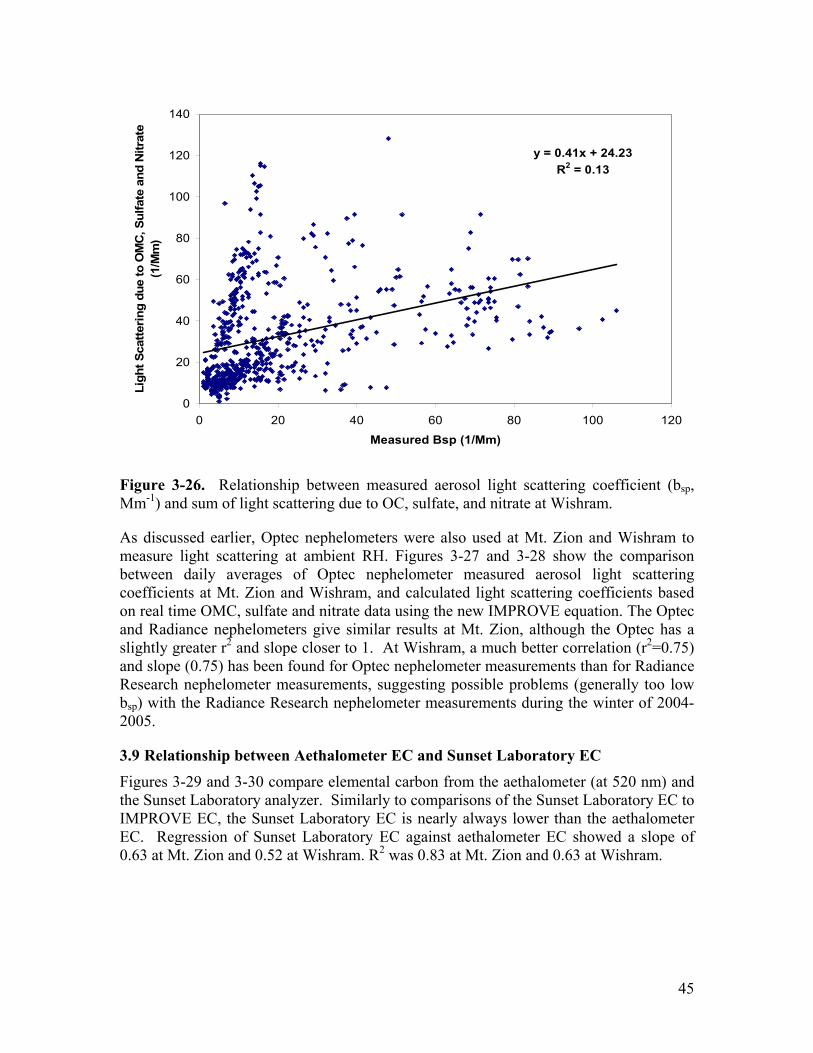
45
y = 0.41x + 24.23R2 = 0.13
0
20
40
60
80
100
120
140
0 20 40 60 80 100 120
Measured Bsp (1/Mm)
Ligh
t Sca
tterin
g du
e to
OM
C, S
ulfa
te a
nd N
itrat
e (1
/Mm
)
Figure 3-26. Relationship between measured aerosol light scattering coefficient (bsp, Mm-1) and sum of light scattering due to OC, sulfate, and nitrate at Wishram.
As discussed earlier, Optec nephelometers were also used at Mt. Zion and Wishram to measure light scattering at ambient RH. Figures 3-27 and 3-28 show the comparison between daily averages of Optec nephelometer measured aerosol light scattering coefficients at Mt. Zion and Wishram, and calculated light scattering coefficients based on real time OMC, sulfate and nitrate data using the new IMPROVE equation. The Optec and Radiance nephelometers give similar results at Mt. Zion, although the Optec has a slightly greater r2 and slope closer to 1. At Wishram, a much better correlation (r2=0.75) and slope (0.75) has been found for Optec nephelometer measurements than for Radiance Research nephelometer measurements, suggesting possible problems (generally too low bsp) with the Radiance Research nephelometer measurements during the winter of 2004-2005.
3.9 Relationship between Aethalometer EC and Sunset Laboratory EC Figures 3-29 and 3-30 compare elemental carbon from the aethalometer (at 520 nm) and the Sunset Laboratory analyzer. Similarly to comparisons of the Sunset Laboratory EC to IMPROVE EC, the Sunset Laboratory EC is nearly always lower than the aethalometer EC. Regression of Sunset Laboratory EC against aethalometer EC showed a slope of 0.63 at Mt. Zion and 0.52 at Wishram. R2 was 0.83 at Mt. Zion and 0.63 at Wishram.
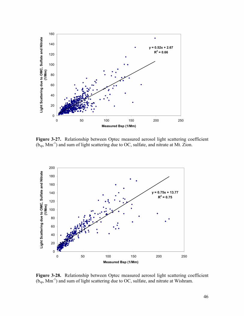
46
y = 0.52x + 2.67R2 = 0.66
0
20
40
60
80
100
120
140
160
0 50 100 150 200 250
Measured Bsp (1/Mm)
Ligh
t Sca
tterin
g du
e to
OM
C, S
ulfa
te a
nd N
itrat
e (1
/Mm
)
Figure 3-27. Relationship between Optec measured aerosol light scattering coefficient (bsp, Mm-1) and sum of light scattering due to OC, sulfate, and nitrate at Mt. Zion.
y = 0.75x + 13.77R2 = 0.75
0
20
40
60
80
100
120
140
160
180
200
0 50 100 150 200 250
Measured Bsp (1/Mm)
Ligh
t Sca
tterin
g du
e to
OM
C, S
ulfa
te a
nd N
itrat
e (1
/Mm
)
Figure 3-28. Relationship between Optec measured aerosol light scattering coefficient (bsp, Mm-1) and sum of light scattering due to OC, sulfate, and nitrate at Wishram.
47
Mt. Zion Sunset Laboratory EC and Aethalometer EC comparison
y = 0.64x - 0.01R2 = 0.83
-0.5
0.0
0.5
1.0
1.5
2.0
2.5
-0.5 0.0 0.5 1.0 1.5 2.0 2.5 3.0
Aethalometer EC (ug/m3)
Suns
et E
C (u
g/m
3)
Figure 3-29. Sunset Laboratory EC concentration (µg/m3) versus aethalometer-derived EC (µg/m3) at Mt. Zion.
Wishram Sunset EC and Athalometer EC comparison
y = 0.45x + 0.04R2 = 0.60
-0.2
0
0.2
0.4
0.6
0.8
1
1.2
1.4
1.6
1.8
2
-0.2 0 0.2 0.4 0.6 0.8 1 1.2 1.4 1.6 1.8 2
Aethalometer EC (520 nm) ug/m3
Suns
et L
abor
ator
y EC
ug/
m3
Figure 3-30. Sunset Laboratory EC concentration (µg/m3) versus aethalometer-derived EC (µg/m3) at Wishram.
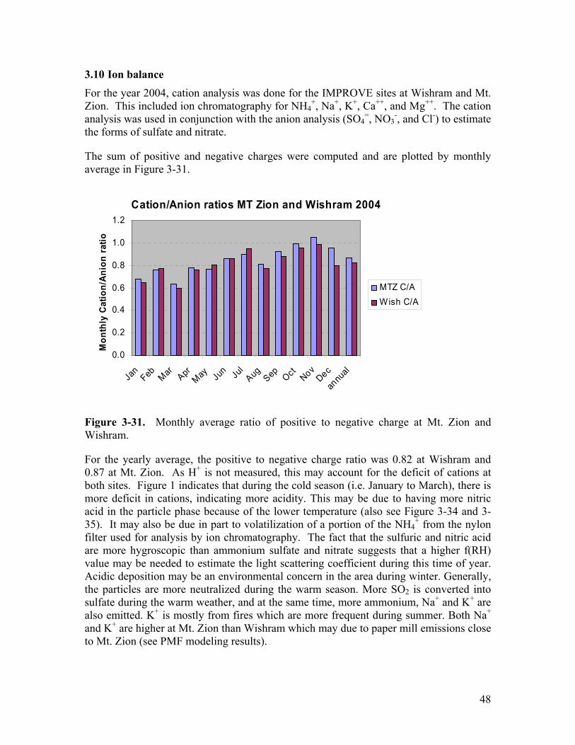
48
3.10 Ion balance For the year 2004, cation analysis was done for the IMPROVE sites at Wishram and Mt. Zion. This included ion chromatography for NH4
+, Na+, K+, Ca++, and Mg++. The cation analysis was used in conjunction with the anion analysis (SO4
=, NO3-, and Cl-) to estimate
the forms of sulfate and nitrate.
The sum of positive and negative charges were computed and are plotted by monthly average in Figure 3-31.
Cation/Anion ratios MT Zion and Wishram 2004
0.0
0.2
0.4
0.6
0.8
1.0
1.2
Jan
Feb Mar AprMay Ju
n Jul
Aug Sep Oct NovDec
annu
al
Mon
thly
Cat
ion/
Anio
n ra
tio
MTZ C/AWish C/A
Figure 3-31. Monthly average ratio of positive to negative charge at Mt. Zion and Wishram.
For the yearly average, the positive to negative charge ratio was 0.82 at Wishram and 0.87 at Mt. Zion. As H+ is not measured, this may account for the deficit of cations at both sites. Figure 1 indicates that during the cold season (i.e. January to March), there is more deficit in cations, indicating more acidity. This may be due to having more nitric acid in the particle phase because of the lower temperature (also see Figure 3-34 and 3-35). It may also be due in part to volatilization of a portion of the NH4
+ from the nylon filter used for analysis by ion chromatography. The fact that the sulfuric and nitric acid are more hygroscopic than ammonium sulfate and nitrate suggests that a higher f(RH) value may be needed to estimate the light scattering coefficient during this time of year. Acidic deposition may be an environmental concern in the area during winter. Generally, the particles are more neutralized during the warm season. More SO2 is converted into sulfate during the warm weather, and at the same time, more ammonium, Na+ and K+ are also emitted. K+ is mostly from fires which are more frequent during summer. Both Na+ and K+ are higher at Mt. Zion than Wishram which may due to paper mill emissions close to Mt. Zion (see PMF modeling results).
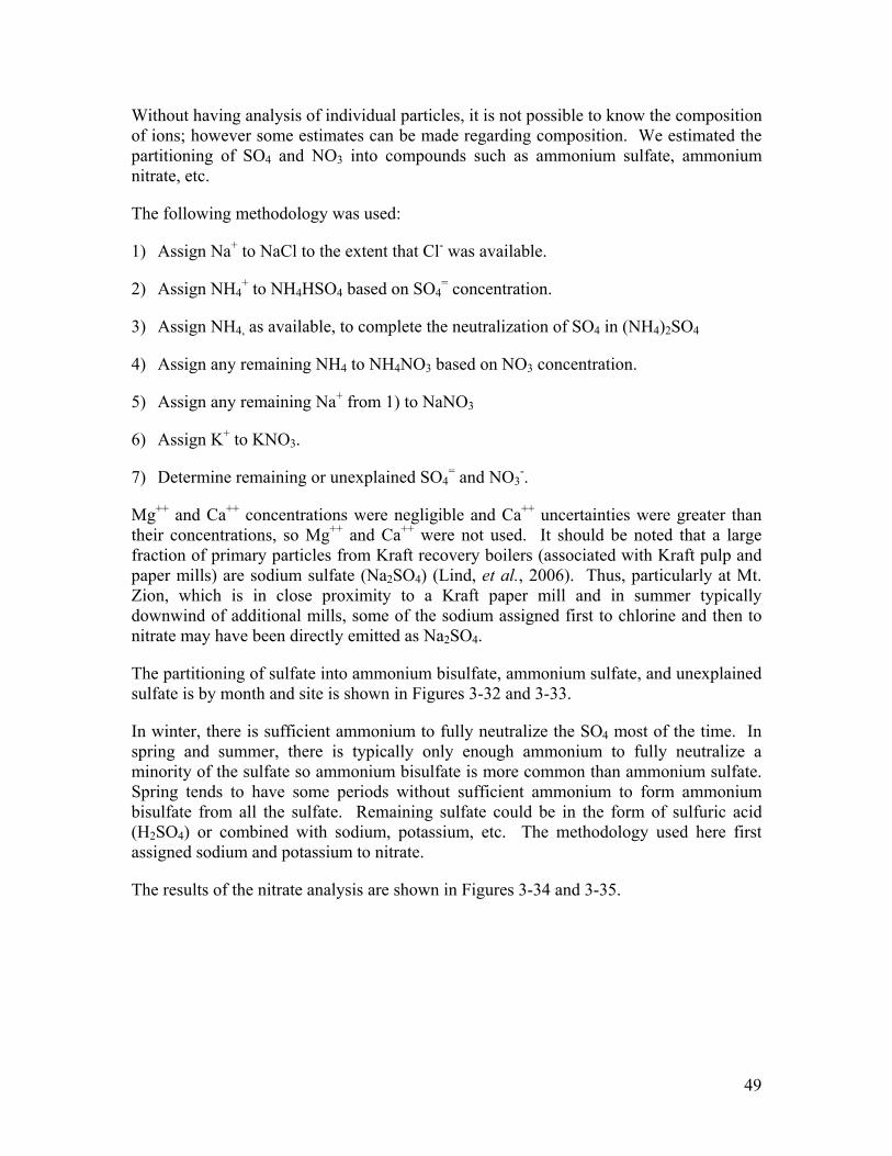
49
Without having analysis of individual particles, it is not possible to know the composition of ions; however some estimates can be made regarding composition. We estimated the partitioning of SO4 and NO3 into compounds such as ammonium sulfate, ammonium nitrate, etc.
The following methodology was used:
1) Assign Na+ to NaCl to the extent that Cl- was available.
2) Assign NH4+ to NH4HSO4 based on SO4
= concentration.
3) Assign NH4, as available, to complete the neutralization of SO4 in (NH4)2SO4
4) Assign any remaining NH4 to NH4NO3 based on NO3 concentration.
5) Assign any remaining Na+ from 1) to NaNO3
6) Assign K+ to KNO3.
7) Determine remaining or unexplained SO4= and NO3
-.
Mg++ and Ca++ concentrations were negligible and Ca++ uncertainties were greater than their concentrations, so Mg++ and Ca++ were not used. It should be noted that a large fraction of primary particles from Kraft recovery boilers (associated with Kraft pulp and paper mills) are sodium sulfate (Na2SO4) (Lind, et al., 2006). Thus, particularly at Mt. Zion, which is in close proximity to a Kraft paper mill and in summer typically downwind of additional mills, some of the sodium assigned first to chlorine and then to nitrate may have been directly emitted as Na2SO4.
The partitioning of sulfate into ammonium bisulfate, ammonium sulfate, and unexplained sulfate is by month and site is shown in Figures 3-32 and 3-33.
In winter, there is sufficient ammonium to fully neutralize the SO4 most of the time. In spring and summer, there is typically only enough ammonium to fully neutralize a minority of the sulfate so ammonium bisulfate is more common than ammonium sulfate. Spring tends to have some periods without sufficient ammonium to form ammonium bisulfate from all the sulfate. Remaining sulfate could be in the form of sulfuric acid (H2SO4) or combined with sodium, potassium, etc. The methodology used here first assigned sodium and potassium to nitrate.
The results of the nitrate analysis are shown in Figures 3-34 and 3-35.
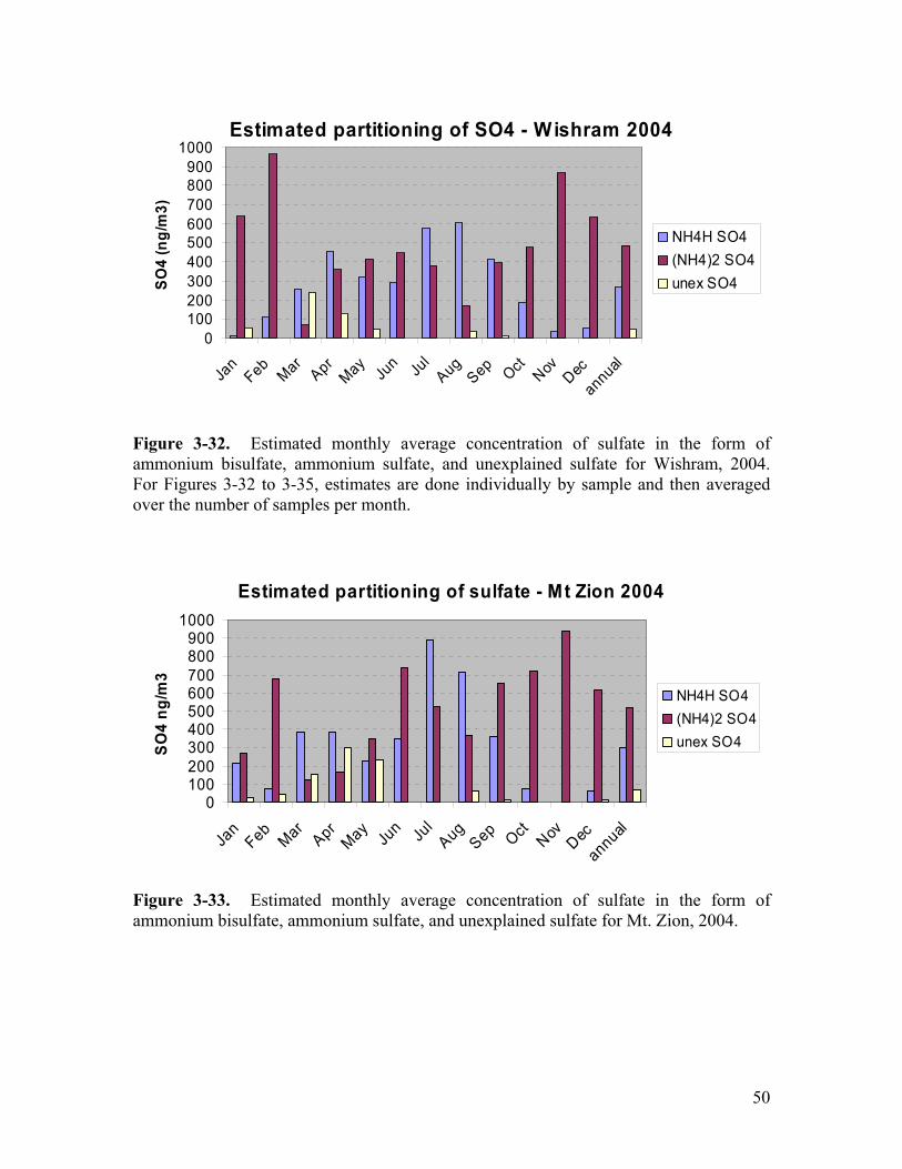
50
Estimated partitioning of SO4 - Wishram 2004
0100200300400500600700800900
1000
Jan
FebMar
AprMay
Jun Ju
lAug
Sep Oct Nov Decannual
SO4
(ng/
m3)
NH4H SO4(NH4)2 SO4unex SO4
Figure 3-32. Estimated monthly average concentration of sulfate in the form of ammonium bisulfate, ammonium sulfate, and unexplained sulfate for Wishram, 2004. For Figures 3-32 to 3-35, estimates are done individually by sample and then averaged over the number of samples per month.
Estimated partitioning of sulfate - Mt Zion 2004
0100200300400500600700800900
1000
Jan
FebMar
AprMay
Jun Ju
lAug
Sep Oct Nov Decannual
SO4
ng/m
3
NH4H SO4(NH4)2 SO4unex SO4
Figure 3-33. Estimated monthly average concentration of sulfate in the form of ammonium bisulfate, ammonium sulfate, and unexplained sulfate for Mt. Zion, 2004.
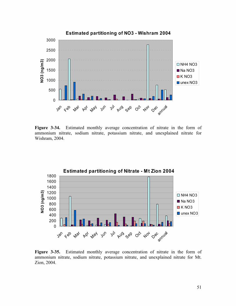
51
Estimated partitioning of NO3 - Wishram 2004
0
500
1000
1500
2000
2500
3000
Jan
FebMar
AprMay
Jun Ju
lAug
Sep Oct Nov Decannual
NO
3 (n
g/m
3)
NH4 NO3Na NO3K NO3unex NO3
Figure 3-34. Estimated monthly average concentration of nitrate in the form of ammonium nitrate, sodium nitrate, potassium nitrate, and unexplained nitrate for Wishram, 2004.
Estimated partitioning of Nitrate - Mt Zion 2004
0200400600800
10001200140016001800
Jan
FebMar
AprMay
Jun Ju
lAug
Sep Oct Nov Decannual
NO
3 (n
g/m
3)
NH4 NO3Na NO3K NO3unex NO3
Figure 3-35. Estimated monthly average concentration of nitrate in the form of ammonium nitrate, sodium nitrate, potassium nitrate, and unexplained nitrate for Mt. Zion, 2004.
52
Ammonium nitrate dominates the nitrate budget in winter and is greater at Wishram than Mt. Zion. From March- September, sodium nitrate and unexplained nitrate (possibly nitric acid - HNO3) are the largest components. Ammonium nitrate averages higher at Wishram than Mt. Zion. Sodium nitrate is higher at Mt. Zion than Wishram. Potassium nitrate is highest in late summer – early fall and is higher at Mt. Zion than Wishram. Annual average concentrations of each component of nitrate and sulfate and their percentage of the total is given in Table 3-3. These results suggest that sources of ammonia affect Wishram more than Mt. Zion (especially in winter) and sources of sodium and potassium affect Mt. Zion more than Wishram (especially in summer).
Table 3-3. Annual average estimated sulfate and nitrate compound concentrations and percentage of total. Concentrations include the sulfate or nitrate mass only and do not include the mass of associated compounds such as ammonium, etc. Note that some sulfate is likely sodium sulfate directly emitted from Kraft recovery boilers.
Wishram Mt. Zion
Compound Concentration of SO4 or NO3 (ng/m3)
Percent Concentration (ng/m3)
Percent
NH4HSO4 270 34 304 34
(NH4)2SO4 488 61 522 59
Unexplained SO4 46 6 65 7
NH4NO3 551 54 379 46
NaNO3 144 15 194 23
KNO3 42 4 93 11
Unexplained NO3 260 27 165 20
3.11 Data Quality Summary Table Table 3-4 presents the authors opinions regarding relative quality of the data collected for the study and its appropriate uses.
53
Table 3-4. Recommended uses and limitations of study measurements.
Instrument Measurement Sites deployed Appropriate Uses Limitations Radiance Research nephelometer
RH controlled Light scattering by particles (Bsp)
9 sites Vertical and horizontal Gradients in haze, temporal patterns
Underestimates haze during higher RH conditions
Optec nephelometer
Light scattering by particles (Bsp)
Wishram,
Mt. Zion
Temporal patterns in haze at east and west ends of gorge
Data flagged under high RH conditions (>90%)
Surface meteorology sensors
Temperature, RH, wind speed, wind direction
All nephelometer sites except Memaloose
Relate nephelometer and aerosol data to source directions, compute f(RH)
IMPROVE sampler
PM2.5 mass and chemical speciation, PM10 mass
Wishram
Mt. Zion
Estimated chemical component contributions to haze, PMF modeling
Data only every third day. Some elements poorly measured (e.g. Na, Cl). No routine cation analysis (e.g. NH4
+) IAS sampler PM2.5 mass and
chemical speciation Sauvie Island, Bonneville Dam, Towal Road
Determine major components contributing to haze at sites with IAS samplers
Limited number of samples, low flow rates, high blank concentrations
Not useful with IMPROVE samples to determine gradients
Sunset laboratory EC/OC analyzer
About 2 hour average EC/OC
Bonneville Dam, Wishram (winter), Mt. Zion (summer-fall)
Time resolved concentration of EC and OC, high time resolved reconstructed extinction, episode analysis
Comparability with filter measurements of EC/OC
Rupprect & Patashnick sulfate analyzer
High time resolved sulfate (1-hour averages used)
Bonneville Dam, Wishram (winter), Mt. Zion (summer-fall)
Sulfate contributions to haze in episode analysis
Poor comparison to filter data at Wishram, but tracks nephelometer scattering during episodes
Rupprect & Patashnick nitrate analyzer
High time resolved nitrate (1-hour averages used)
Bonneville Dam, Wishram (winter), Mt. Zion (summer-fall)
Nitrate contributions to haze in episode analysis
Poor comparison to filter data at Wishram, but tracks nephelometer scattering during episodes
DRUM sampler Size and time (3 hr) resolved PM2.5 chemical composition
Bonneville Dam, Wishram (winter), Mt. Zion (summer-fall)
Time resolved elements for episode analysis, size distribution analysis
Compare poorly with filter data, limited periods of analysis
Aethalometer Light absorbing (elemental) carbon
Wishram
Mt. Zion
High time resolved EC for episode analysis, continuous EC
Calibration issues, scattering particle interference
54
The surface meteorology data, the nephelometer data and the IMPROVE data are of sufficiently high quality for quantitative use to determine extinction budgets, source-receptor relationships, and to evaluate meteorological and air quality model performance.
The other measurements should be considered more semi-quantitative and are useful for timing of changes in aerosol components and determination of main components contributing to high nephelometer measurements. They are most useful for episode analysis. The high-time resolution data did an adequate job of reconstructing light scattering measured by the nephelometers.
55
4. Attribution
4.1 PMF analysis To help identify the sources of aerosols in the Columbia River Gorge, the Positive Matrix Factorization (PMF) receptor model was applied to the 24-hr integrated aerosol chemical composition data obtained at the Columbia River Gorge through the Interagency Monitoring of Protected Visual Environments (IMPROVE) program (sites Mt. Zion and Wishram) during the years 2003-2004. PMF was applied to each site to generate profiles of source factors. Normalized source profiles and the quantitative source contributions for each resolved factor were calculated. The major sources that contribute to the aerosol loadings and light extinction in the Columbia River Gorge were identified.
4.1.1 Methodology PMF is a statistical method that identifies a user specified number of source profiles (i.e. relative composition particle species for each source) and source strengths for each sample period that reduces the difference between measured and PMF fitted mass concentration [Kim et al., 2003; Liu et al., 2003; Kim and Hopke, 2004]. Equations 1 – 3 show the major steps of the model calculation.
EGFX += (1)
where: X (n * Sp) = a matrix of observed fine particulate species concentrations with the dimensions of number of observations by the number of species
G (n * f) = a matrix of source contributions by observation day with the dimensions of number of observations by the number of factors
F (f * Sp) = a matrix of source profiles with the dimensions of number of factors by the number of species
E (n * Sp) = a matrix of random errors with the dimensions of number of observations by number of species
The F and G matrices of the final solution are then normalized according to the following equations to determine the quantitative source contributions (Ci, µg/m3)) and profiles for each source (Si, µg/µg).
i
iji FM
FS = (2)
where: Si = the row of the source profile matrix for source i
Fij = the source profile value for specie j of source i
FMi = the calculated average total fine mass contribution for source i
ikii FMGC *= (3)
where: Ci = the column of the source contribution matrix for source i
Gki = the source contribution on day k for source i
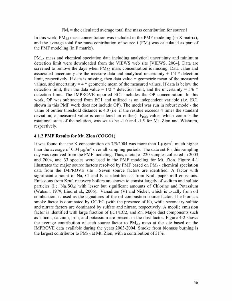
56
FMi = the calculated average total fine mass contribution for source i
In this work, PM2.5 mass concentration was included in the PMF modeling (in X matrix), and the average total fine mass contribution of source i (FMi) was calculated as part of the PMF modeling (in F matrix).
PM2.5 mass and chemical speciation data including analytical uncertainty and minimum detection limit were downloaded from the VIEWS web site [VIEWS, 2004]. Data are screened to remove the days when PM2.5 mass concentration is missing. Data value and associated uncertainty are the measure data and analytical uncertainty + 1/3 * detection limit, respectively. If data is missing, then data value = geometric mean of the measured values, and uncertainty = 4 * geometric mean of the measured values. If data is below the detection limit, then the data value = 1/2 * detection limit, and the uncertainty = 5/6 * detection limit. The IMPROVE reported EC1 includes the OP concentration. In this work, OP was subtracted from EC1 and utilized as an independent variable (i.e. EC1 shown in this PMF work does not include OP). The model was run in robust mode - the value of outlier threshold distance is 4.0 (i.e. if the residue exceeds 4 times the standard deviation, a measured value is considered an outlier). Fpeak value, which controls the rotational state of the solution, was set to be -1.0 and -1.5 for Mt. Zion and Wishram, respectively.
4.1.2 PMF Results for Mt. Zion (COGO1)
It was found that the K concentration on 7/5/2004 was more than 1 µg/m3, much higher than the average of 0.04 µg/m3 over all sampling periods. The data set for this sampling day was removed from the PMF modeling. Thus, a total of 220 samples collected in 2003 and 2004, and 33 species were used in the PMF modeling for Mt. Zion. Figure 4-1 illustrates the major source factors resolved by PMF based on PM2.5 chemical speciation data from the IMPROVE site . Seven source factors are identified. A factor with significant amount of Na, Cl and K is identified as from Kraft paper mill emissions. Emissions from Kraft recovery boilers are shown to consist largely of sodium and sulfate particles (i.e. Na2SO4) with lesser but significant amounts of Chlorine and Potassium (Watson, 1979, Lind et al., 2006). Vanadium (V) and Nickel, which is usually from oil combustion, is used as the signatures of the oil combustion source factor. The biomass smoke factor is dominated by OC/EC (with the presence of K), while secondary sulfate and nitrate factors are dominated by sulfate and nitrate, respectively. A mobile emission factor is identified with large fraction of EC1/EC2, and Zn. Major dust components such as silicon, calcium, iron, and potassium are present in the dust factor. Figure 4-2 shows the average contribution of each source factor to PM2.5 mass at the site based on the IMPROVE data available during the years 2003-2004. Smoke from biomass burning is the largest contributor to PM2.5 at Mt. Zion, with a contribution of 31%.
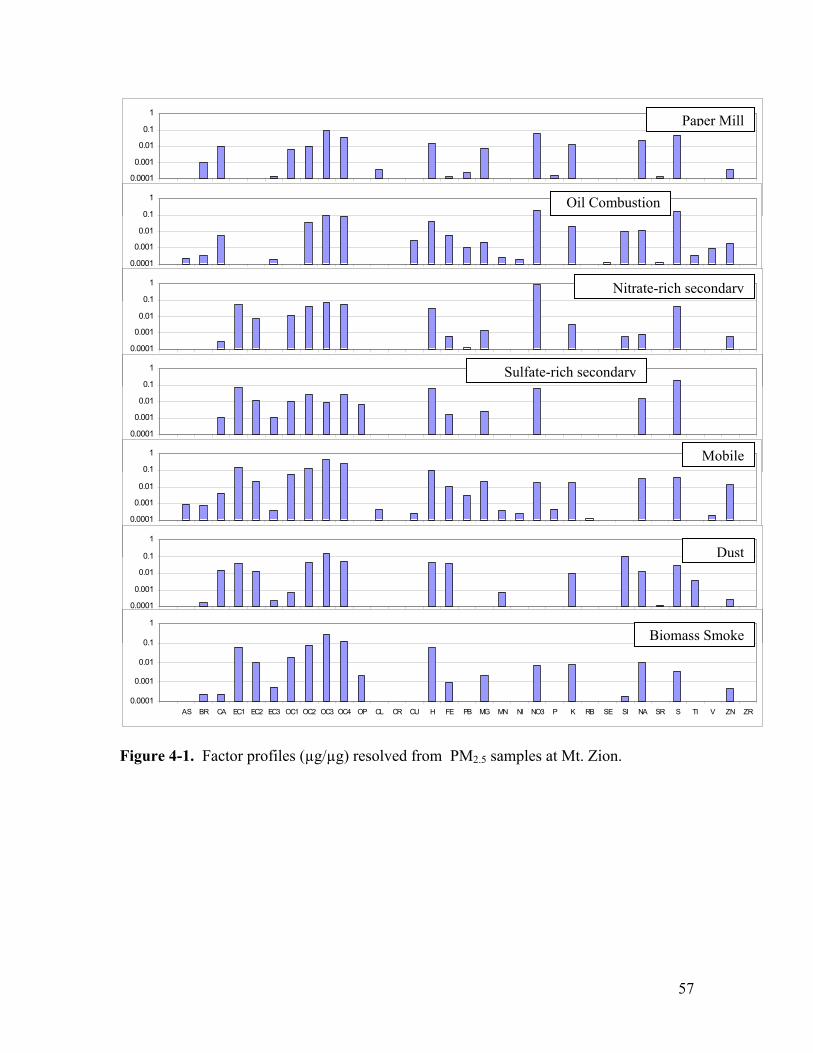
57
0.0001
0.001
0.01
0.1
1
AS BR CAEC1
EC2EC3
OC1OC2
OC3OC4 OP CL CR CU H FE PB MG MN NI
NO3 P K RB SE SINA SR S TI V ZN ZR
0.0001
0.001
0.01
0.1
1
AS BR CAEC1
EC2EC3
OC1OC2
OC3OC4 OP CL CR CU H FE PB MG MN NI
NO3 P K RB SE SINA SR S TI V ZN ZR
0.0001
0.001
0.01
0.1
1
AS BR CAEC1
EC2EC3
OC1OC2
OC3OC4 OP CL CR CU H FE PB MG MN NI
NO3 P K RB SE SINA SR S TI V ZN ZR
0.0001
0.001
0.01
0.1
1
AS BR CAEC1
EC2EC3
OC1OC2
OC3OC4 OP CL CR CU H FE PB MG MN NI
NO3 P K RB SE SINA SR S TI V ZN ZR
0.0001
0.001
0.01
0.1
1
AS BR CAEC1
EC2EC3
OC1OC2
OC3OC4 OP CL CR CU H FE PB MG MN NI
NO3 P K RB SE SINA SR S TI V ZN ZR
0.0001
0.001
0.01
0.1
1
AS BR CAEC1
EC2EC3
OC1OC2
OC3OC4 OP CL CR CU H FE PB MG MN NI
NO3 P K RB SE SINA SR S TI V ZN ZR
0.0001
0.001
0.01
0.1
1
AS BR CA EC1 EC2 EC3 OC1 OC2 OC3 OC4 OP CL CR CU H FE PB MG MN NI NO3 P K RB SE SI NA SR S TI V ZN ZR
Figure 4-1. Factor profiles (µg/µg) resolved from PM2.5 samples at Mt. Zion.
Dust
Oil Combustion
Sulfate-rich secondary
Paper Mill
Nitrate-rich secondary
Mobile
Biomass Smoke
58
Paper Mill14%
Oil Combustion8%
Nitrate-rich Secondary
13%
Sulfate-rich Secondary
16%
Mobile5%
Dust13%
Biomass Smoke31%
Figure 4-2. Average contribution of each factor to PM2.5 mass at Mt. Zion.
Figure 4-3 shows the time series of contributions of each source to PM2.5 mass during the years 2003-2004. They indicate that oil and sulfate factors contribute most during the summer season, while nitrate has the highest contribution in the winter. Smoke and dust are episodic sources – big peaks during dust and fire events, while the contributions of mobile and paper mill emissions are relatively constant throughout the year.
4.1.3 PMF Results for Wishram (CORI1) A total of 237 samples collected in 2003 and 2004, and 33 species were used in the PMF modeling for Wishram. Figure 4-4 illustrates the major source factors resolved by PMF based on PM2.5 chemical speciation data. Five source factors are identified for Wishram. As with Mt. Zion, a biomass smoke factor is identified as dominated by OC/EC (with the presence of K), and secondary sulfate and nitrate factors are dominated by sulfate and nitrate, respectively. A mobile emission factor is identified with large fraction of EC1/EC2 and organics, as well as Zn and Pb. A dust factor dominated by mineral components silicon, calcium, iron, and potassium is identified. Figure 4-5 shows the average contribution of each source factor to PM2.5 mass at Wishram based on the IMPROVE data available during the years 2003-2004. Smoke from biomass burning is the largest contributor to PM2.5 at Wishram, with a contribution of 29%, followed by secondary sulfate and nitrate. Figure 4-6 shows the time series of contributions of each source to PM2.5 mass during the years 2003-2004. The sulfate factor contributes most during the summer season, while nitrate contributes most in the winter. Smoke and dust are episodic sources with big peaks during dust and fire pollution events, while the contribution of mobile sources is relatively constant throughout the year.

59
0
1
2
3
4
5
6
12/30/2002 5/29/2003 10/26/2003 3/24/2004 8/21/2004 1/18/2005Date
Con
cent
ratio
n (u
g/m
3)Paper Mill
(a)
0
0.5
1
1.5
2
2.5
3
12/30/2002 5/29/2003 10/26/2003 3/24/2004 8/21/2004 1/18/2005Date
Con
cent
ratio
n (u
g/m
3)
Oil Combustion
(b)
Figure 4-3. Time series of: a) paper mill, b) oil combustion, c) nitrate-rich secondary, d) sulfate-rich secondary, e) mobile, f) dust, and g) biomass smoke source contributions at Mt. Zion.

60
0
1
2
3
4
5
6
7
8
9
12/30/2002 5/29/2003 10/26/2003 3/24/2004 8/21/2004 1/18/2005Date
Con
cent
ratio
n (u
g/m
3)Nitrate-rich Secondary
(c)
0
0.5
1
1.5
2
2.5
3
3.5
4
4.5
5
12/30/2002 5/29/2003 10/26/2003 3/24/2004 8/21/2004 1/18/2005Date
Con
cent
ratio
n (u
g/m
3)
Sulfate-rich Secondary
(d)
Figure 4-3. Continued.

61
0
0.2
0.4
0.6
0.8
1
1.2
12/30/2002 5/29/2003 10/26/2003 3/24/2004 8/21/2004 1/18/2005Date
Con
cent
ratio
n (u
g/m
3)Mobile
(e)
0
1
2
3
4
5
6
7
12/30/2002 5/29/2003 10/26/2003 3/24/2004 8/21/2004 1/18/2005Date
Con
cent
ratio
n (u
g/m
3)
Dust
(f)
Figure 4-3. Continued.

62
0
2
4
6
8
10
12
14
16
12/30/2002 5/29/2003 10/26/2003 3/24/2004 8/21/2004 1/18/2005Date
Con
cent
ratio
n (u
g/m
3)
Biomass Smoke
(g)
Figure 4-3. Continued.

63
0.0001
0.001
0.01
0.1
1
AS BR CAEC1
EC2EC
3OC1
OC2OC3
OC4 OP CL CR CU H FE PB MG MN NINO3 P K RB SE SI
NA SR S TI V ZN ZR
0.0001
0.001
0.01
0.1
1
AS BR CAEC1
EC2
EC3
OC1OC2
OC3OC4 OP CL CR CU H FE PB MG MN NI
NO3 P K RB SE SINA SR S TI V ZN ZR
0.0001
0.001
0.01
0.1
1
AS BR CAEC
1EC2
EC3
OC1OC2
OC3OC4 OP CL CR CU H FE PB MG MN NI
NO3 P K RB SE SINA SR S TI V ZN ZR
0.0001
0.001
0.01
0.1
1
AS BR CAEC1
EC2
EC3
OC1OC2
OC3OC4 OP CL CR CU H FE PB MG MN NI
NO3 P K RB SE SINA SR S TI V ZN ZR
0.0001
0.001
0.01
0.1
1
AS BR CA EC1 EC2 EC3 OC1 OC2 OC3 OC4 OP CL CR CU H FE PB MG MN NI NO3 P K RB SE SI NA SR S TI V ZN ZR
Figure 4-4. Factor profiles (µg/µg) resolved from PM2.5 samples at Wishram.
Sulfate-rich secondary
Biomass Smoke
Mobile
Dust
Nitrate-rich secondary
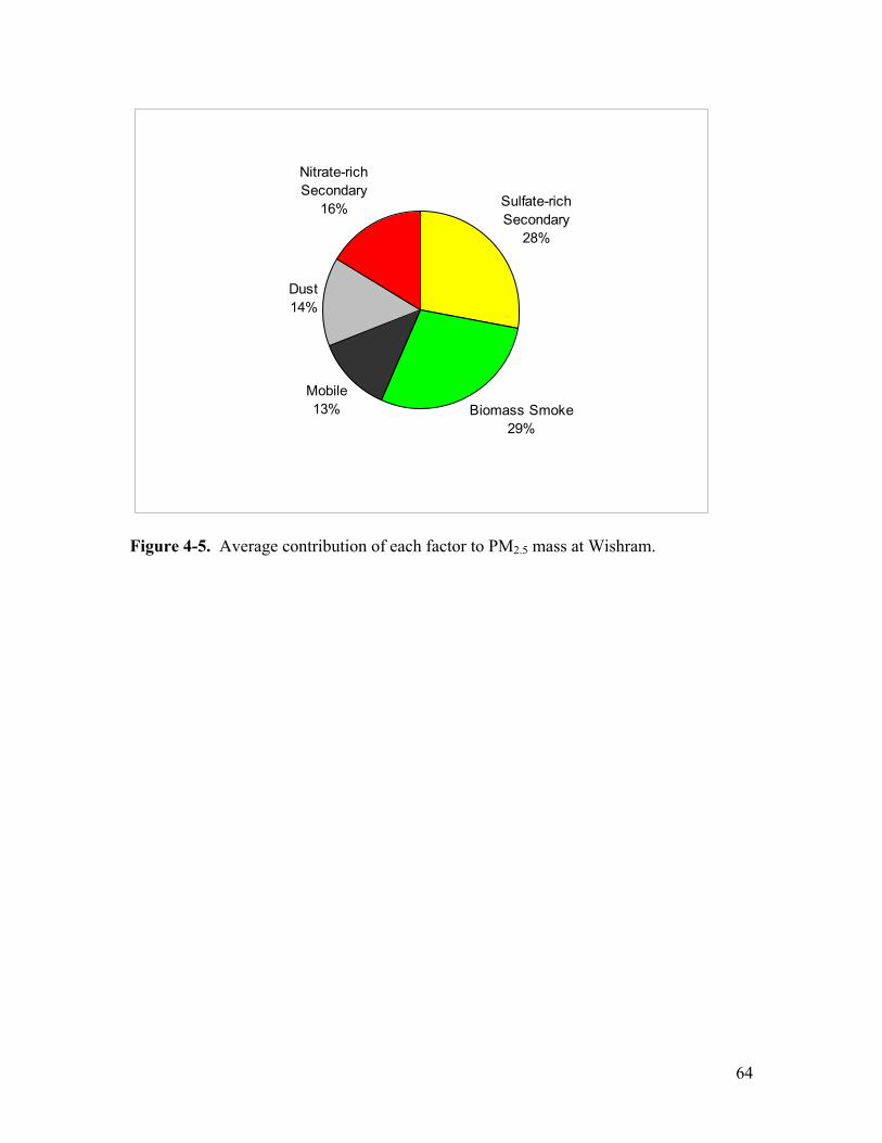
64
Sulfate-rich Secondary
28%
Biomass Smoke29%
Mobile13%
Dust14%
Nitrate-rich Secondary
16%
Figure 4-5. Average contribution of each factor to PM2.5 mass at Wishram.
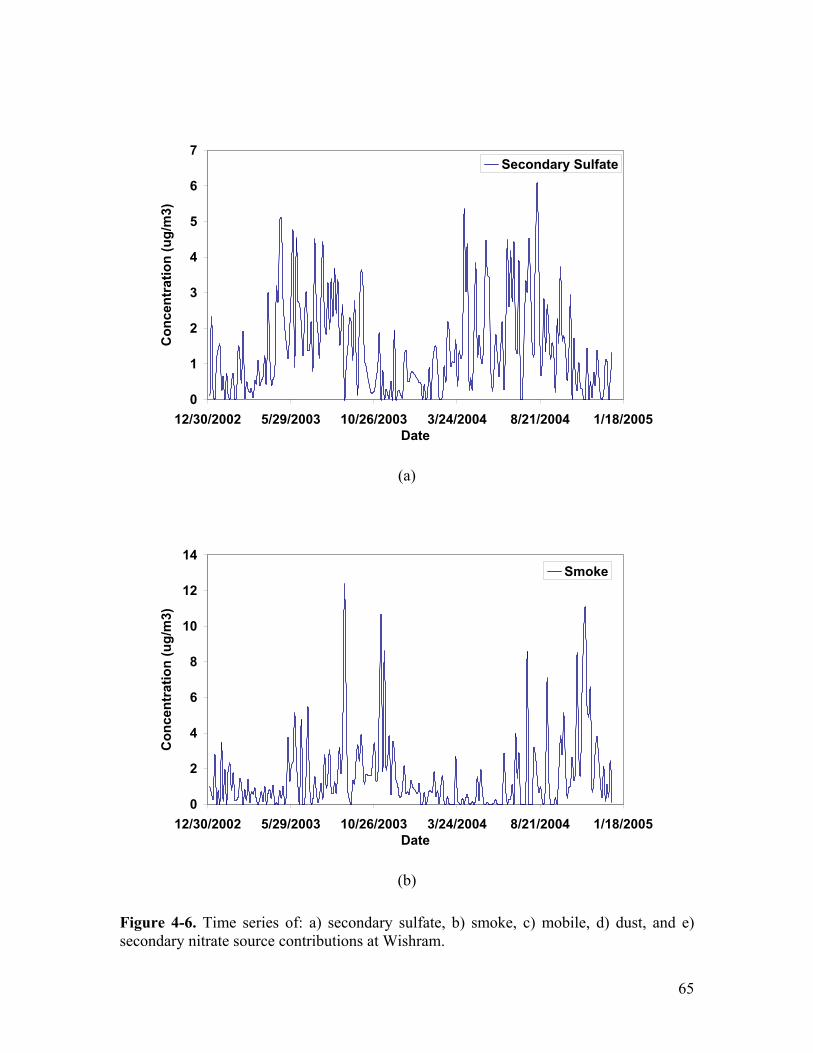
65
0
1
2
3
4
5
6
7
12/30/2002 5/29/2003 10/26/2003 3/24/2004 8/21/2004 1/18/2005Date
Con
cent
ratio
n (u
g/m
3)Secondary Sulfate
(a)
0
2
4
6
8
10
12
14
12/30/2002 5/29/2003 10/26/2003 3/24/2004 8/21/2004 1/18/2005Date
Con
cent
ratio
n (u
g/m
3)
Smoke
(b)
Figure 4-6. Time series of: a) secondary sulfate, b) smoke, c) mobile, d) dust, and e) secondary nitrate source contributions at Wishram.
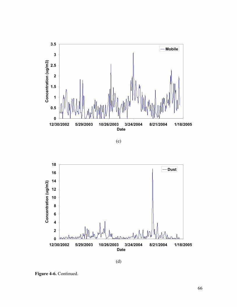
66
0
0.5
1
1.5
2
2.5
3
3.5
12/30/2002 5/29/2003 10/26/2003 3/24/2004 8/21/2004 1/18/2005Date
Con
cent
ratio
n (u
g/m
3)Mobile
(c)
0
2
4
6
8
10
12
14
16
18
12/30/2002 5/29/2003 10/26/2003 3/24/2004 8/21/2004 1/18/2005Date
Con
cent
ratio
n (u
g/m
3)
Dust
(d)
Figure 4-6. Continued.
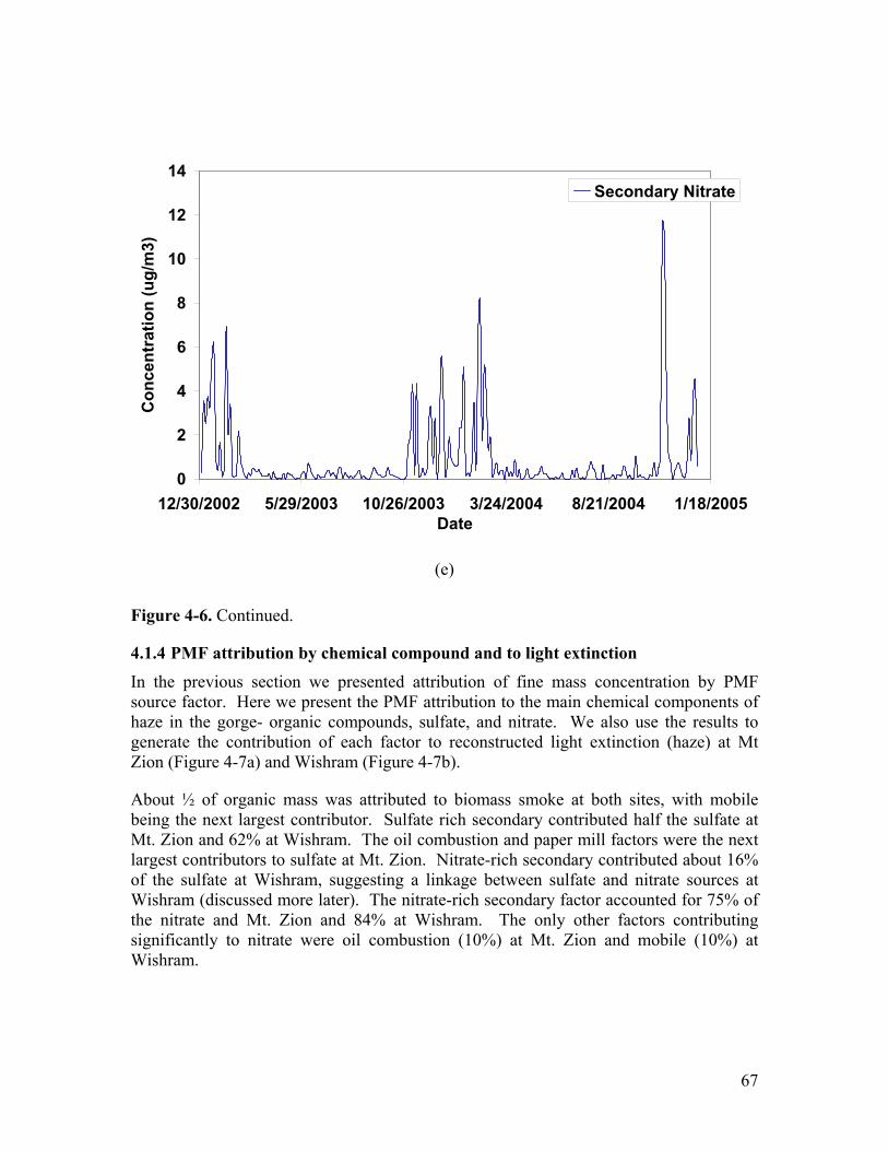
67
0
2
4
6
8
10
12
14
12/30/2002 5/29/2003 10/26/2003 3/24/2004 8/21/2004 1/18/2005Date
Con
cent
ratio
n (u
g/m
3)
Secondary Nitrate
(e)
Figure 4-6. Continued.
4.1.4 PMF attribution by chemical compound and to light extinction In the previous section we presented attribution of fine mass concentration by PMF source factor. Here we present the PMF attribution to the main chemical components of haze in the gorge- organic compounds, sulfate, and nitrate. We also use the results to generate the contribution of each factor to reconstructed light extinction (haze) at Mt Zion (Figure 4-7a) and Wishram (Figure 4-7b).
About ½ of organic mass was attributed to biomass smoke at both sites, with mobile being the next largest contributor. Sulfate rich secondary contributed half the sulfate at Mt. Zion and 62% at Wishram. The oil combustion and paper mill factors were the next largest contributors to sulfate at Mt. Zion. Nitrate-rich secondary contributed about 16% of the sulfate at Wishram, suggesting a linkage between sulfate and nitrate sources at Wishram (discussed more later). The nitrate-rich secondary factor accounted for 75% of the nitrate and Mt. Zion and 84% at Wishram. The only other factors contributing significantly to nitrate were oil combustion (10%) at Mt. Zion and mobile (10%) at Wishram.

68
Paper Mill6%
Oil Combustion10%
Nitrate-rich Secondary
75%
Dust0%
Sulfate-rich Secondary
7%
Biomass Smoke1%Mobile
1%Paper Mill
7%
Oil Combustion
10%
Nitrate-rich Secondary
27%
Sulfate-rich Secondary
22%
Mobile5%
Dust6%
Biomass Smoke
15%
CM8%
Mobile14%
Biomass Smoke53%
Sulfate-rich Secondary
4%
Dust10%
Paper Mill6%
Oil Combustion5%
Nitrate-rich Secondary
8%
Paper Mill11%
Oil Combustion20%
Nitrate-rich Secondary
8%
Sulfate-rich Secondary
50%
Dust6%
Biomass Smoke2%
Mobile3%
(a)
Figure 4-7. Contribution of each source factor to organic mass, sulfate, nitrate, and reconstructed light extinction at: a) Mt. Zion and b) Wishram.
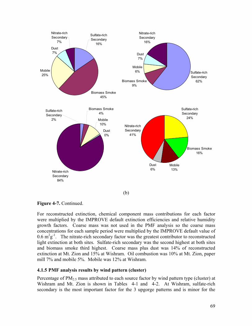
69
Sulfate-rich Secondary
24%
Biomass Smoke16%
Mobile13%
Dust6%
Nitrate-rich Secondary
41%
Biomass Smoke4%
Mobile10%
Dust0%
Nitrate-rich Secondary
84%
Sulfate-rich Secondary
2%
Sulfate-rich Secondary
62%Biomass Smoke9%
Mobile6%
Dust7%
Nitrate-rich Secondary
16%
Biomass Smoke45%
Mobile25%
Dust7%
Nitrate-rich Secondary
7%
Sulfate-rich Secondary
16%
(b)
Figure 4-7. Continued.
For reconstructed extinction, chemical component mass contributions for each factor were multiplied by the IMPROVE default extinction efficiencies and relative humidity growth factors. Coarse mass was not used in the PMF analysis so the coarse mass concentrations for each sample period were multiplied by the IMPROVE default value of 0.6 m2g-1. The nitrate-rich secondary factor was the greatest contributor to reconstructed light extinction at both sites. Sulfate-rich secondary was the second highest at both sites and biomass smoke third highest. Coarse mass plus dust was 14% of reconstructed extinction at Mt. Zion and 15% at Wishram. Oil combustion was 10% at Mt. Zion, paper mill 7% and mobile 5%. Mobile was 12% at Wishram.
4.1.5 PMF analysis results by wind pattern (cluster) Percentage of PM2.5 mass attributed to each source factor by wind pattern type (cluster) at Wishram and Mt. Zion is shown in Tables 4-1 and 4-2. At Wishram, sulfate-rich secondary is the most important factor for the 3 upgorge patterns and is minor for the

70
winter downgorge. Biomass smoke is the largest contributor to the light downgorge pattern, and is about 30% of PM2.5 mass for the light and moderate upgorge and winter downgorge patterns. The mobile factor is most important for light upgorge and light downgorge. The dust factor is highest for the usually summertime moderate and strong upgorge patterns. Nitrate rich secondary is the largest factor for the winter downgorge pattern, is also substantial for light downgorge, and is minor for the upgorge patterns. It should be noted that the upgorge wind paterns have slightly higher PM2.5 mass at Mt. Zion than Wishram and the downgorge patterns have higher PM mass at Wishram- thus a higher percentage at one site may or may not imply a higher concentration of PM2.5 mass.
This summary implies most sulfate at Wishram is from the west, most nitrate is from the east, and biomass smoke comes from both east and west.
Table 4-1. Percentage of PM2.5 mass attributed to each source factor by wind pattern type (cluster) at Wishram.
Percentage of PM2.5
Light upgorge
(1)
Moderate upgorge
(2)
Strong upgorge
(3)
Light downgorge
(4)
Winter downgorge
(5)
Sulfate-rich secondary 33 33 44 16 9
Biomass smoke 31 28 19 37 33
Mobile 17 12 10 16 9
Dust 15 22 22 12 6
Nitrate-rich secondary 5 5 5 19 44
Table 4-2. Percentage of PM2.5 mass attributed to each source factor by wind pattern type (cluster) at Mt. Zion.
Percentage of PM2.5
Light upgorge
(1)
Moderate upgorge
(2)
Strong upgorge
(3)
Light downgorge
(4)
Winter downgorge
(5)
Paper Mill 14 15 19 10 6
Oil Combustion 8 14 14 3 1
Nitrate-rich secondary 10 7 9 12 34
Sulfate-rich secondary 17 13 16 10 19
Mobile 5 4 5 5 3
Dust 14 18 12 16 5
Biomass smoke 32 29 25 43 32

71
At Mt. Zion, the biomass smoke factor has the largest contribution to PM2.5 mass for all wind patterns except winter downgorge, where nitrate-rich secondary is slightly higher. The paper mill factor is highest for the upgorge types, which is reasonable because multiple paper mills are west of Mt. Zion. Sulfate-rich secondary ranges from 10-19 percent, is associated with both upgorge and downgorge flow, and is marginally highest for winter downgorge. This result appears to conflict with the result for Wishram for which winter downgorge has the lowest sulfate factor contribution. However it could be that sources between Wishram and Mt. Zion are contributing to higher sulfate there for wind type 5 or that emissions of SO2 upwind of the gorge have not converted a large fraction of the SO2 to sulfate by the time the emissions reach Wishram (but convert more during transport to Mt. Zion). Also as we shall soon see, the nitrate-rich secondary factor at Wishram contains significant amounts of sulfate as well.
The oil combustion factor is highest for moderate and strong upgorge and near zero for the downgorge wind patterns. The dust factor is significant for all but the winter downgorge (winter only) factor. The mobile factor is small for all wind patterns. The nitrate factor is associated mainly with downgorge flow.
4.1.5.a Sulfate attribution by wind field type Here we give results of the PMF analysis specific to attribution of particulate sulfur to PMF factors (Tables 4-3 and 4-4). At Wishram for upgorge winds about 70-80% of the sulfate is attributed to the secondary sulfate factor. Smaller percentages are associated with biomass smoke, mobile, and dust factors, with smoke factor associated sulfate higher during downgorge flow. An interesting finding is that for wind type 5, winter downgorge, over one-half of the sulfate at Wishram is attributed to the secondary-nitrate factor. This suggests that the source or sources contributing to secondary nitrate also have substantial sulfate associated with them. (The mass contribution to nitrate from this factor is much higher than to sulfate). The Boardman power plant is a large source of SO2 and NOX (precursor compounds to particulate sulfate and nitrate). Because the nitrate factor has substantial sulfate attributed to it is reasonable to suggest that the “secondary nitrate” factor may be largely a “Boardman power plant” factor. This is supported by the fact that the contribution from this factor is highest when winds are from the east (toward Wishram from the Boardman power plant).
The analysis does not “prove” that Boardman is responsible for a large fraction of the haze in the gorge in winter. Measurements that may have lead to much stronger evidence of impact were not funded. However, it should be noted that Boardman emits 66% of the SO2 by point sources in Oregon and 34% of the NOx. The most typical winter flow patterns would transport the Boardman emissions through the gorge. Thus, it is not unreasonable to expect that Boardman contributes substantially to winter time sulfate and nitrate in the gorge.
The sulfate attribution at Mt. Zion (Table 4-4) also shows a nitrate-rich secondary factor containing some sulfate that is most important for downgorge flows. The mass contribution to sulfate for this factor is about ½ at Mt. Zion as it is at Wishram, but the profile (ratio of nitrate to sulfate) is about the same at both locations. The sulfate-rich secondary source at Mt. Zion is higher than at Wishram (over twice in terms of mass
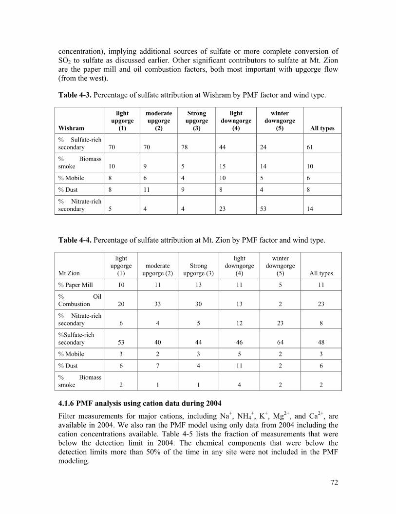
72
concentration), implying additional sources of sulfate or more complete conversion of SO2 to sulfate as discussed earlier. Other significant contributors to sulfate at Mt. Zion are the paper mill and oil combustion factors, both most important with upgorge flow (from the west).
Table 4-3. Percentage of sulfate attribution at Wishram by PMF factor and wind type.
Wishram
light upgorge
(1)
moderate upgorge
(2)
Strong upgorge
(3)
light downgorge
(4)
winter downgorge
(5) All types
% Sulfate-rich secondary 70 70 78 44 24 61
% Biomass smoke 10 9 5 15 14 10
% Mobile 8 6 4 10 5 6
% Dust 8 11 9 8 4 8
% Nitrate-rich secondary 5 4 4 23 53 14
Table 4-4. Percentage of sulfate attribution at Mt. Zion by PMF factor and wind type.
Mt Zion
light upgorge
(1) moderate
upgorge (2) Strong
upgorge (3)
light downgorge
(4)
winter downgorge
(5) All types
% Paper Mill 10 11 13 11 5 11
% Oil Combustion 20 33 30 13 2 23
% Nitrate-rich secondary 6 4 5 12 23 8
%Sulfate-rich secondary 53 40 44 46 64 48
% Mobile 3 2 3 5 2 3
% Dust 6 7 4 11 2 6
% Biomass smoke 2 1 1 4 2 2
4.1.6 PMF analysis using cation data during 2004 Filter measurements for major cations, including Na+, NH4
+, K+, Mg2+, and Ca2+, are available in 2004. We also ran the PMF model using only data from 2004 including the cation concentrations available. Table 4-5 lists the fraction of measurements that were below the detection limit in 2004. The chemical components that were below the detection limits more than 50% of the time in any site were not included in the PMF modeling.

73
Table 4-5. Fraction of measurements that were below detection limits in 2004.
Code Elements Mt. Zion Wishram CommentsAL Aluminum 0.55 0.41 Not included in PMFAS Arsenic 0.22 0.41BR Bromine 0.00 0.00CA Calcium 0.00 0.00EC1 Elemental Carbon 1 0.03 0.02EC2 Elemental Carbon 2 0.18 0.08EC3 Elemental Carbon 3 0.80 0.76 Not included in PMFOC1 Organic Carbon 1 0.44 0.41OC2 Organic Carbon 2 0.04 0.07OC3 Organic Carbon 3 0.01 0.07OC4 Organic Carbon 4 0.00 0.05OP Organic Carbon Pyrolized 0.73 0.59 Not included in PMFCHL Chloride 0.02 0.22CL Chlorine 0.69 0.61 Not included in PMFCR Chromium 0.37 0.34CU Copper 0.02 0.01H Hydrogen 0.00 0.00FE Iron 0.00 0.00PB Lead 0.02 0.03MG Magnesium 0.78 0.79 Not included in PMFMN Manganese 0.06 0.00NI Nickel 0.35 0.52
NO3 Nitrate 0.00 0.04P Phosphorus 0.96 0.99 Not included in PMFK Potassium 0.00 0.00
RB Rubidium 0.51 0.48 Not included in PMFSE Selenium 0.22 0.24SI Silicon 0.10 0.01NA Sodium 0.72 0.76 Not included in PMFSR Strontium 0.15 0.13S Sulfur 0.00 0.00TI Titanium 0.03 0.01V Vanadium 0.19 0.23
ZN Zinc 0.00 0.00ZR Zirconium 0.95 0.87 Not included in PMF
NA+ Sodium Ion 0.04 0.09NH4+ Ammonium 0.08 0.11
K+ Potassium Ion 0.02 0.12MG++ Magnesium Ion 0.38 0.44CA++ Calcium Ion 0.95 0.92 Not included in PMF
Figure 4-8 and 4-9 show the source profiles resolved by PMF using only data from 2004. Table 4-6 lists the PMF results using data from 2003 and 2004, results based on data from 2004 only including cations Na+, NH4
+, K+, and Mg2+, as well as results from Dr. Keith Rose’s analysis using data from 1996-1998. Similar results were found from these different modeling runs. Secondary sulfate contributions were lower using only 2004’s data mainly due to the reason that some measured NH4
+ concentrations were quite low (close or equal to zero). It is not clear if this is due to analysis problems. A paper mill factor, which has an almost identical source profile as for Mt. Zion, was identified for

74
Wishram using only 2004’s data. It was blended with other factors using data from 2003-2004 without cations. This may be due to the reason that there are large uncertainties in XRF sodium measurements (which is used in PMF modeling for 2003-2004), while the IC sodium ion (Na+) measurement (used in PMF modeling for 2004 only) is more accurate. The paper mill factor at Wishram was associated with winds from the west. A mixed combustion factor was identified for Mt. Zion based on 2004 only modeling, which includes emissions from both mobile and oil combustion sources. An unknown factor with very high K+ concentration was identified for 2004 only modeling in Mt. Zion. We are not sure if this is due to measurement uncertainties. But the total K concentrations based on XRF measurements were much lower than IC measured K+ during the days when this factor was important.
The 2004 with cation PMF results and the 2003-2004 (no cation) results do not lead to substantial differences in source contributions. The main differences are: 1) blending of the mobile and oil combustion sources at Mt. Zion and 2) appearance of a paper mill factor at Wishram, probably containing primary sodium sulfate, coincident with a reduced secondary sulfate factor.
4.2 Episode analysis
4.2.1 November 2004 Episode An extended episode of high bsp at all sites occurred during early-mid November 2004. Daily averaged bsp for all nephelometers (Radiance Research heated nephelometers) is shown in Figure 4-10. Unless noted otherwise all nephelometer data in the episode analysis section is from the heated Radiance Research nephelometers. Also shown is the cluster number. National Weather Service sites in eastern Washington and eastern Oregon (Walla Walla, Pasco, and Pendleton) reported light winds, high RH and smoke/haze and fog leading up to and during the episode. The episode started as light upgorge flow on November 6 turned to light downgorge flow on November 7-8. Bsp levels dipped slightly with light upgorge flow on November 9 then rose with downgorge flow on November 10, which continued for a few days with a gradual reduction in daily average bsp. All sites except Sauvie Island and Steigerwald had daily average bsp peaking on November 10. Towal Road and Wishram had daily average bsp of over 200 Mm-1 on November 10, and bsp on that date generally decreased from east to west. Time resolved sulfate (SO4), nitrate (NO3), and OC/EC were available for Bonneville and Mt. Zion for this period (although Mt Zion OC/EC was only available for the early part of the episode). Hourly averaged bsp, SO4, NO3, and OC at Bonneville and Mt. Zion for November 7- November 15 are shown in Figures 4-11a and 4-11b.
This episode had elevated concentrations of sulfate, nitrate, and organic carbon. Sulfate concentrations were as high as 10 µg/m3 at Mt Zion and 8 µg/m3 at Bonneville. Nitrate reached hourly average concentrations of over 9 µg/m3 at both locations. Peak OC concentrations were about 8 µg/m3 at Bonneville and 7 µg/m3 at Mt. Zion and concentrations were generally higher at Bonneville than at Mt. Zion.
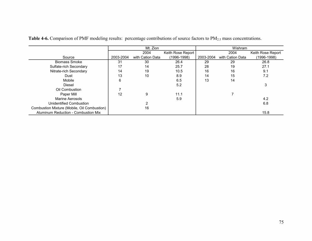
75
Table 4-6. Comparison of PMF modeling results: percentage contributions of source factors to PM2.5 mass concentrations.
2004 Keith Rose Report 2004 Keith Rose Report2003-2004 with Cation Data (1996-1998) 2003-2004 with Cation Data (1996-1998)
Biomass Smoke 31 30 26.4 29 29 26.8Sulfate-rich Secondary 17 14 25.7 28 19 27.1Nitrate-rich Secondary 14 19 10.5 16 16 9.1
Dust 13 10 8.9 14 15 7.2Mobile 6 6.5 13 14Diesel 5.2 3
Oil Combustion 7Paper Mill 12 9 11.1 7
Marine Aerosols 5.9 4.2Unidentified Combustion 2 6.8
Combustion Mixture (Mobile, Oil Combustion) 16Aluminum Reduction - Combustion Mix 15.8
Mt. Zion Wishram
Source

76
0.0001
0.001
0.01
0.1
1
AS BR CA EC1 EC2 OC1 OC2 OC3 OC4 CHL CR CU H FE PB MN NI NO3 K SE SI SR S TI V ZN NA+ NH4+ K+ MG++
0.0001
0.001
0.01
0.1
1
AS BR CA EC1 EC2 OC1 OC2 OC3 OC4 CHL CR CU H FE PB MN NI NO3 K SE SI SR S TI V ZN NA+ NH4+ K+ MG++
0.0001
0.001
0.01
0.1
1
AS BR CA EC1 EC2 OC1 OC2 OC3 OC4 CHL CR CU H FE PB MN NI NO3 K SE SI SR S TI V ZN NA+ NH4+ K+ MG++
0.0001
0.001
0.01
0.1
1
AS BR CA EC1 EC2 OC1 OC2 OC3 OC4 CHL CR CU H FE PB MN NI NO3 K SE SI SR S TI V ZN NA+ NH4+ K+ MG++
0.0001
0.001
0.01
0.1
1
AS BR CA EC1 EC2 OC1 OC2 OC3 OC4 CHL CR CU H FE PB MN NI NO3 K SE SI SR S TI V ZN NA+ NH4+ K+ MG++
0.0001
0.001
0.01
0.1
1
AS BR CA EC1 EC2 OC1 OC2 OC3 OC4 CHL CR CU H FE PB MN NI NO3 K SE SI SR S TI V ZN NA+ NH4+ K+ MG++
0.0001
0.001
0.01
0.1
1
AS BR CA EC1 EC2 OC1 OC2 OC3 OC4 CHL CR CU H FE PB MN NI NO3 K SE SI SR S TI V ZN NA+ NH4+ K+ MG++
Figure 4-8. Source profiles for Mt. Zion based on PMF modeling for 2004 only.
Combustion Mixture
Biomass Smoke
Paper Mill
Sulfate-rich Secondary
Dust
Nitrate-rich Secondary
Unknown
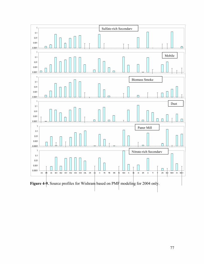
77
0.0001
0.001
0.01
0.1
1
AS BR CA EC1 EC2 OC1 OC2 OC3 OC4 CHL CR CU H FE PB MN NI NO3 K SE SI SR S TI V ZN NA+ NH4+ K+ MG++
0.0001
0.001
0.01
0.1
1
AS BR CA EC1 EC2 OC1 OC2 OC3 OC4 CHL CR CU H FE PB MN NI NO3 K SE SI SR S TI V ZN NA+ NH4+ K+ MG++
0.0001
0.001
0.01
0.1
1
AS BR CA EC1 EC2 OC1 OC2 OC3 OC4 CHL CR CU H FE PB MN NI NO3 K SE SI SR S TI V ZN NA+ NH4+ K+ MG++
0.0001
0.001
0.01
0.1
1
AS BR CA EC1 EC2 OC1 OC2 OC3 OC4 CHL CR CU H FE PB MN NI NO3 K SE SI SR S TI V ZN NA+ NH4+ K+ MG++
0.0001
0.001
0.01
0.1
1
AS BR CA EC1 EC2 OC1 OC2 OC3 OC4 CHL CR CU H FE PB MN NI NO3 K SE SI SR S TI V ZN NA+ NH4+ K+ MG++
0.0001
0.001
0.01
0.1
1
AS BR CA EC1 EC2 OC1 OC2 OC3 OC4 CHL CR CU H FE PB MN NI NO3 K SE SI SR S TI V ZN NA+ NH4+ K+ MG++
Figure 4-9. Source profiles for Wishram based on PMF modeling for 2004 only.
Sulfate-rich Secondary
Biomass Smoke
Dust
Paper Mill
Nitrate-rich Secondary
Mobile
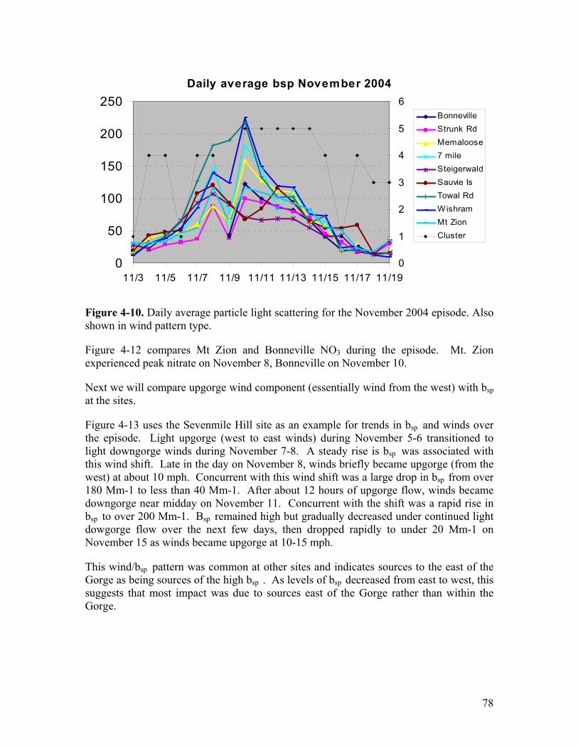
78
Daily average bsp November 2004
0
50
100
150
200
250
11/3 11/5 11/7 11/9 11/11 11/13 11/15 11/17 11/190
1
2
3
4
5
6BonnevilleStrunk RdMemaloose7 mileSteigerwaldSauvie IsTowal RdWishramMt ZionCluster
Figure 4-10. Daily average particle light scattering for the November 2004 episode. Also shown in wind pattern type.
Figure 4-12 compares Mt Zion and Bonneville NO3 during the episode. Mt. Zion experienced peak nitrate on November 8, Bonneville on November 10.
Next we will compare upgorge wind component (essentially wind from the west) with bsp at the sites.
Figure 4-13 uses the Sevenmile Hill site as an example for trends in bsp and winds over the episode. Light upgorge (west to east winds) during November 5-6 transitioned to light downgorge winds during November 7-8. A steady rise is bsp was associated with this wind shift. Late in the day on November 8, winds briefly became upgorge (from the west) at about 10 mph. Concurrent with this wind shift was a large drop in bsp from over 180 Mm-1 to less than 40 Mm-1. After about 12 hours of upgorge flow, winds became downgorge near midday on November 11. Concurrent with the shift was a rapid rise in bsp to over 200 Mm-1. Bsp remained high but gradually decreased under continued light dowgorge flow over the next few days, then dropped rapidly to under 20 Mm-1 on November 15 as winds became upgorge at 10-15 mph.
This wind/bsp pattern was common at other sites and indicates sources to the east of the Gorge as being sources of the high bsp . As levels of bsp decreased from east to west, this suggests that most impact was due to sources east of the Gorge rather than within the Gorge.
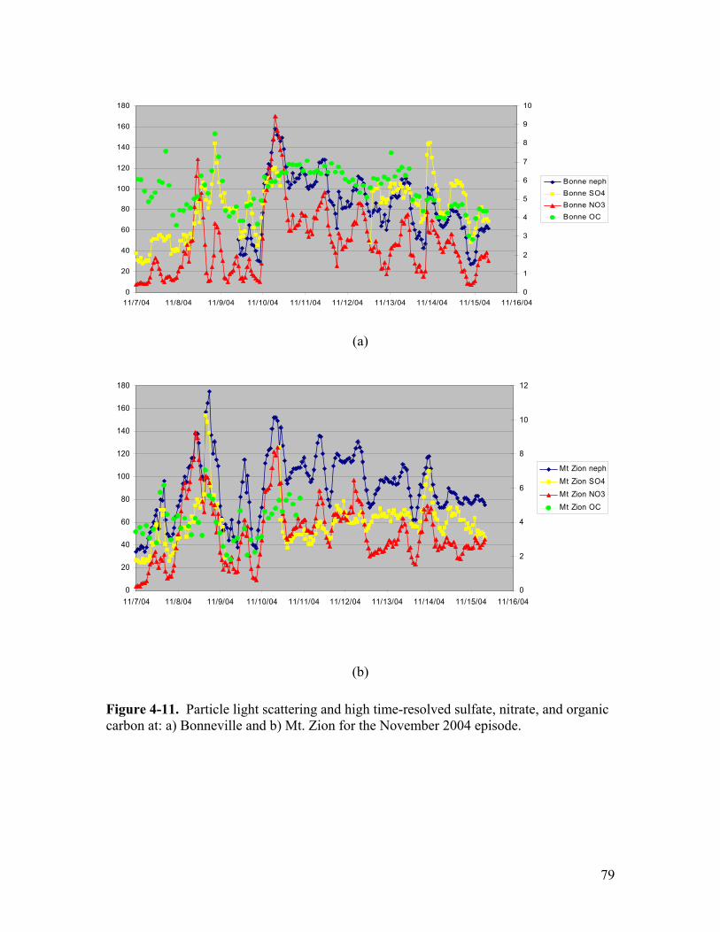
79
0
20
40
60
80
100
120
140
160
180
11/7/04 11/8/04 11/9/04 11/10/04 11/11/04 11/12/04 11/13/04 11/14/04 11/15/04 11/16/040
1
2
3
4
5
6
7
8
9
10
Bonne nephBonne SO4Bonne NO3Bonne OC
(a)
0
20
40
60
80
100
120
140
160
180
11/7/04 11/8/04 11/9/04 11/10/04 11/11/04 11/12/04 11/13/04 11/14/04 11/15/04 11/16/040
2
4
6
8
10
12
Mt Zion nephMt Zion SO4Mt Zion NO3Mt Zion OC
(b)
Figure 4-11. Particle light scattering and high time-resolved sulfate, nitrate, and organic carbon at: a) Bonneville and b) Mt. Zion for the November 2004 episode.

80
0
1
2
3
4
5
6
7
8
9
10
11/7/04 11/8/04 11/9/04 11/10/04 11/11/04 11/12/04 11/13/04 11/14/04 11/15/04 11/16/04
NO
3 (u
g/m
3)Mt Zion NO3Bonne NO3
Figure 4-12. Time series of high time-resolved nitrate at Mt. Zion and Bonneville for the November 2004 episode.
0
40
80
120
160
200
240
11/5 11/6 11/7 11/8 11/9 11/10 11/11 11/12 11/13 11/14 11/15 11/16 11/17
7 m
ile b
sp (M
m-1
)
-10
-5
0
5
10
15
20
7 m
ile u
pgor
ge w
ind
(mph
)
7 mile bsp 7 mile W
Figure 4-13. Time series of bsp and upgorge wind component at Sevenmile Hill during the November 2004 episode.

81
4.2.1.a PMF results for episode PMF results are available for Wishram and Mt. Zion. Table 4-7 gives the percentage of fine mass apportioned to each source averaged over the peak episode days with IMPROVE samples (November 8, November 11, and November 14).
Table 4-7. Percentage of fine mass apportioned by PMF to each source factor at Wishram and Mt. Zion (for the samples on November 8, 11, and 14, 2004).
Sulfate rich
Biomass burning
Mobile Dust Nitrate rich
Oil combustion
Paper mill
Mt. Zion 9.8 41.1 3.1 3.3 37.4 1.2 4.1
Wishram 2.4 43.3 7.4 1.6 45.3 NA NA
The bulk of the fine mass was attributed to the biomass burning and nitrate-rich secondary factors.
4.2.2 February 2004 episode This episode was characterized by strong synoptic scale high pressure systems to the east of the study area. This resulted in an east to west pressure gradient and downgorge flow (cluster 5) every day from February 10-17, 2004. The downgorge flow varied in strength with variations in the pressure gradients. Figure 4-14 shows the time series of hourly averaged light scattering at the nephelometer sites.
Bsp rose rapidly (from <20 Mm-1 to 80-100 Mm-1) at all sites during from evening of February 10 to early morning on February 11 and were similar in magnitude at all sites early February 11. This rise coincided with an increase in downgorge at the sites, suggesting transport down gorge from the east (Figure 4-15). Bsp at all but the easternmost sites decreased substantially from the morning of February 11 to midday February 12. This decrease in bsp occurred while downgorge winds were strong (Figure 4-15), suggesting a dilution of aerosol. A rise in bsp then followed, peaking in early evening on February 13 at the western sites and gradually declining the rest of the episode. The rise to a peak at the western sites occurred as downgorge winds eased, possibly reducing the dilution effect. At the eastern sites of Towal Road, Wishram, and Memaloose, bsp continued to rise until the late hours of February 14 to the early hours of February 15. During portions of the episode there were small gradients of bsp throughout the gorge and while later in the episode, large gradients existed.
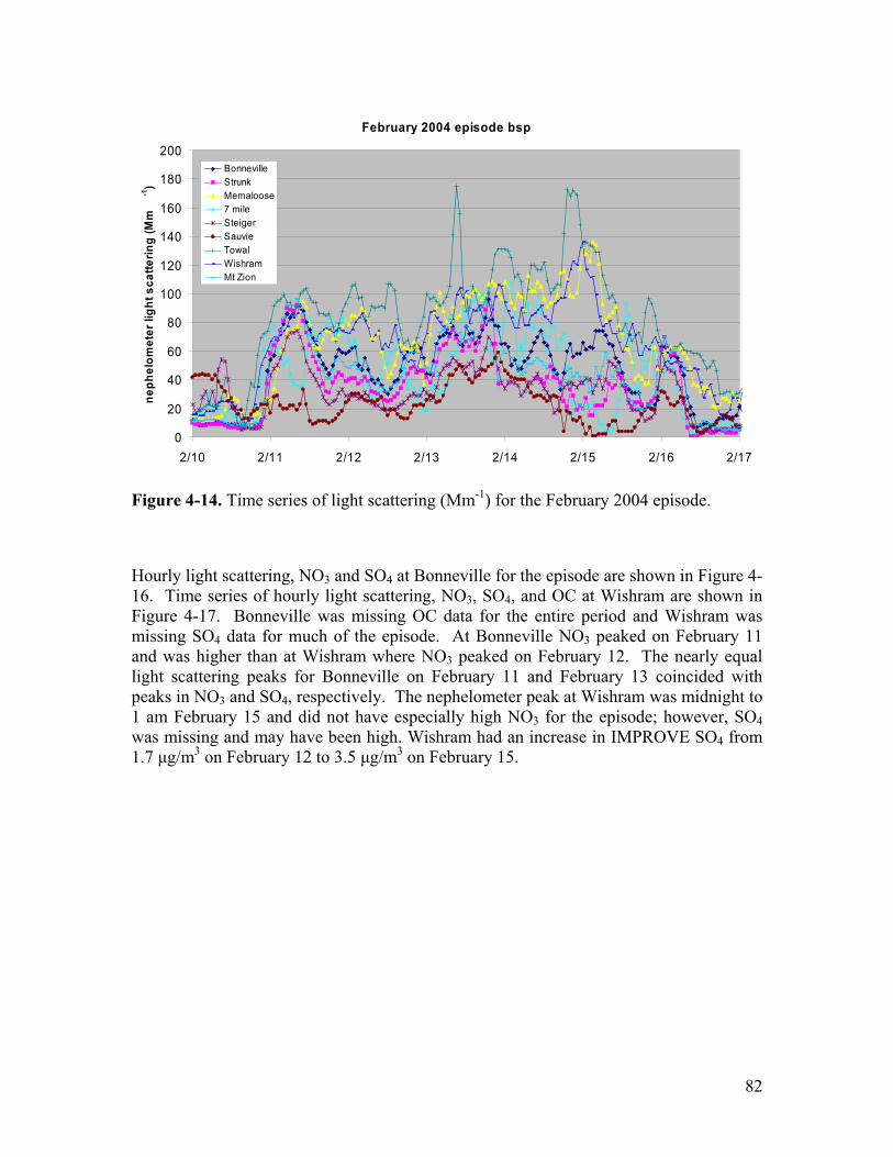
82
February 2004 episode bsp
0
20
40
60
80
100
120
140
160
180
200
2/10 2/11 2/12 2/13 2/14 2/15 2/16 2/17
neph
elom
eter
ligh
t sca
tterin
g (M
m-1
)BonnevilleStrunkMemaloose7 mileSteigerSauvieTowalWishramMt Zion
Figure 4-14. Time series of light scattering (Mm-1) for the February 2004 episode.
Hourly light scattering, NO3 and SO4 at Bonneville for the episode are shown in Figure 4-16. Time series of hourly light scattering, NO3, SO4, and OC at Wishram are shown in Figure 4-17. Bonneville was missing OC data for the entire period and Wishram was missing SO4 data for much of the episode. At Bonneville NO3 peaked on February 11 and was higher than at Wishram where NO3 peaked on February 12. The nearly equal light scattering peaks for Bonneville on February 11 and February 13 coincided with peaks in NO3 and SO4, respectively. The nephelometer peak at Wishram was midnight to 1 am February 15 and did not have especially high NO3 for the episode; however, SO4 was missing and may have been high. Wishram had an increase in IMPROVE SO4 from 1.7 µg/m3 on February 12 to 3.5 µg/m3 on February 15.
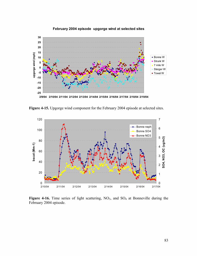
83
February 2004 episode upgorge wind at selected sites
-25
-20
-15
-10
-5
0
5
10
15
20
25
30
2/9/04 2/10/04 2/11/04 2/12/04 2/13/04 2/14/04 2/15/04 2/16/04 2/17/04 2/18/04 2/19/04
upgo
rge
win
d (m
ph)
Bonne WStrunk W7 mile WSteiger WTowal W
Figure 4-15. Upgorge wind component for the February 2004 episode at selected sites.
0
20
40
60
80
100
120
2/10/04 2/11/04 2/12/04 2/13/04 2/14/04 2/15/04 2/16/04 2/17/04
bsca
t (M
m-1
)
0
1
2
3
4
5
6
7
SO4,
NO
3, O
C (u
g/m
3)
Bonne nephBonne SO4Bonne NO3
Figure 4-16. Time series of light scattering, NO3, and SO4 at Bonneville during the February 2004 episode.
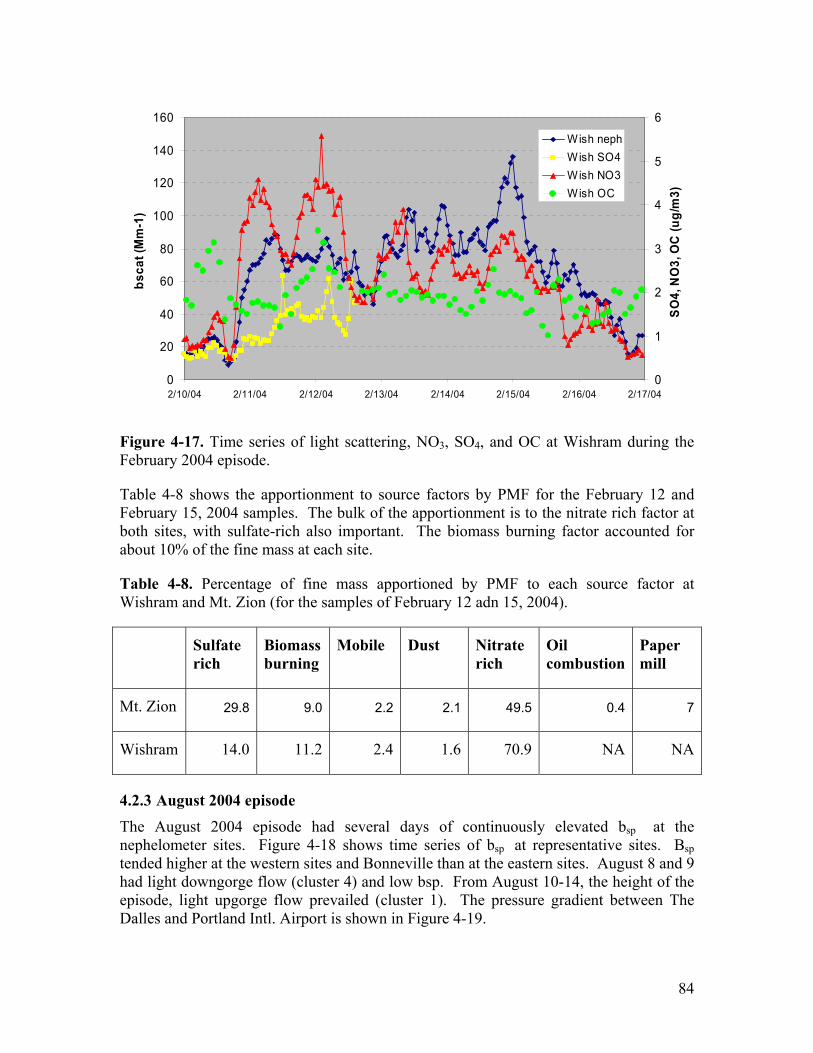
84
0
20
40
60
80
100
120
140
160
2/10/04 2/11/04 2/12/04 2/13/04 2/14/04 2/15/04 2/16/04 2/17/04
bsca
t (M
m-1
)
0
1
2
3
4
5
6
SO4,
NO
3, O
C (u
g/m
3)
Wish nephWish SO4Wish NO3Wish OC
Figure 4-17. Time series of light scattering, NO3, SO4, and OC at Wishram during the February 2004 episode.
Table 4-8 shows the apportionment to source factors by PMF for the February 12 and February 15, 2004 samples. The bulk of the apportionment is to the nitrate rich factor at both sites, with sulfate-rich also important. The biomass burning factor accounted for about 10% of the fine mass at each site.
Table 4-8. Percentage of fine mass apportioned by PMF to each source factor at Wishram and Mt. Zion (for the samples of February 12 adn 15, 2004).
Sulfate rich
Biomass burning
Mobile Dust Nitrate rich
Oil combustion
Paper mill
Mt. Zion 29.8 9.0 2.2 2.1 49.5 0.4 7
Wishram 14.0 11.2 2.4 1.6 70.9 NA NA
4.2.3 August 2004 episode
The August 2004 episode had several days of continuously elevated bsp at the nephelometer sites. Figure 4-18 shows time series of bsp at representative sites. Bsp tended higher at the western sites and Bonneville than at the eastern sites. August 8 and 9 had light downgorge flow (cluster 4) and low bsp. From August 10-14, the height of the episode, light upgorge flow prevailed (cluster 1). The pressure gradient between The Dalles and Portland Intl. Airport is shown in Figure 4-19.
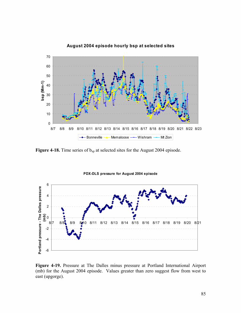
85
August 2004 episode hourly bsp at selected sites
0
10
20
30
40
50
60
70
8/7 8/8 8/9 8/10 8/11 8/12 8/13 8/14 8/15 8/16 8/17 8/18 8/19 8/20 8/21 8/22 8/23
bsp
(Mm
-1)
Bonneville Memaloose Wishram Mt Zion
Figure 4-18. Time series of bsp at selected sites for the August 2004 episode.
PDX-DLS pressure for August 2004 episode
-6
-4
-2
0
2
4
6
8/7 8/8 8/9 8/10 8/11 8/12 8/13 8/14 8/15 8/16 8/17 8/18 8/19 8/20 8/21
Port
land
pre
ssur
e - T
he D
alle
s pr
essu
re
(mb)
Figure 4-19. Pressure at The Dalles minus pressure at Portland International Airport (mb) for the August 2004 episode. Values greater than zero suggest flow from west to east (upgorge).

86
The pressure gradient was downgorge at the beginning of the episode, explaining the light downgorge flow observed. During August 10, the pressure gradient and flow became light upgorge and the bsp increased.
Figure 4-20 shows a time series of bsp, reconstructed bsp, and estimated bsp due to sulfate, nitrate, and organic carbon at Bonneville for the episode. Measured and reconstructed scattering compare well both in magnitude and trend. Reconstructed bsp was due about equally to sulfate and organic carbon, with a very minor contribution from nitrate.
Bonneville bsp, SO4, OC August episode
0
10
20
30
40
50
60
8/8 8/9 8/10 8/11 8/12 8/13 8/14 8/15 8/16 8/17 8/18 8/19 8/20 8/21
Bsc
at (M
m-1
)
Bonne neph Bonne Recon bs Bonne Rec SO4 bs Bonne Rec OC bs Bonne Rec NO3 bs
Figure 4-20. Bsp, reconstructed bsp, and estimated bsp due to sulfate, nitrate, and organic carbon during the August 2004 episode.
Figure 4-21 shows organic carbon concentration at IMPROVE sites in Washington, Idaho, and Oregon for August 13, 2004. The Wishram and Mt. Zion IMPROVE samples are not available for this date. OC concentrations were generally between 2 and 4 µg/m3, with over 8 µg/m3 at Sawtooth Wilderness Area. This suggests impacts from fires in the region. Figure 4-22 shows sulfate levels at IMPROVE sites in the Pacific Northwest for August 16, 2004 (Wishram and Mt. Zion again missing). Increased levels of sulfate are seen at sites in Washington and Oregon in the central and northern Cascades, Puget Sound and Olympic National Park. The high-time resolution sulfate monitor at Mt. Zion (data not shown) gave much lower values than the one at Bonneville, possibly due to a problem with the monitor at Mt. Zion.
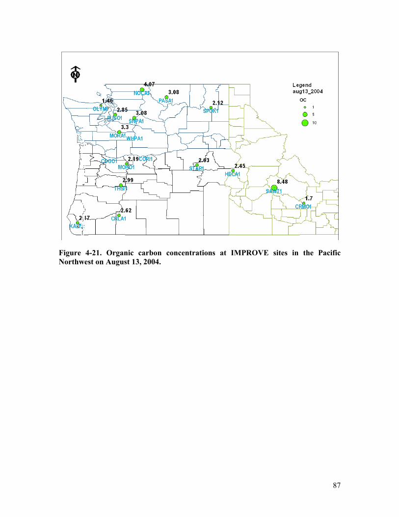
87
Figure 4-21. Organic carbon concentrations at IMPROVE sites in the Pacific Northwest on August 13, 2004.

88
Figure 4-22. Sulfate concentrations at IMPROVE sites in the Pacific Northwest on August 16, 2004.
4.2.4 July 2004 episode The episode began with a light downgorge flow as the pressure was higher at The Dalles than Portland (Figure 4-21). The pressure gradient changed direction late on July 24 and intensified on July 25 leading to upgorge flow the remainder of the episode. Time series of bsp, sulfate, organic carbon, and nitrate at Bonneville and Mt. Zion are shown in Figures 4-24 and 4-25.
Organic carbon and sulfate are significant at both Bonneville and Mt. Zion. As is typical in summer nitrate is low. Time series plots separately comparing bsp, sulfate, and organic carbon at Bonneville and Mt. Zion are shown in Figures 4-26 to 4-28. Bsp, sulfate, and OC track well and are quite similar in magnitude for the two sites except for July 31 when sulfate and bsp are much higher at Mt. Zion. The DRUM data at Mt. Zion (Figure 4-29) and Bonneville show increases in fine sodium concurrent with increases in fine sulfur. From the PMF analysis and source profile data (which indicates that emissions from Kraft recovery boilers consist largely of sodium sulfate) this suggests significant paper mill impact to particulate sulfur (sulfate) at Mt. Zion and Bonneville during this time period.

89
Portland to Dalles Pressure Gradient July 04 episode
-3-2-101234567
7/20 7/21 7/22 7/23 7/24 7/25 7/26 7/27 7/28 7/29 7/30 7/31 8/1
KPD
X-K
DLS
pre
ssur
e (m
b)
Figure 4-23. Pressure at Portland International Airport minus pressure at The Dalles during the July 2004 episode.
Bonneville July 2004 episode
0
10
20
30
40
50
60
70
80
7/22/04 7/23/04 7/24/04 7/25/04 7/26/04 7/27/04 7/28/04 7/29/04 7/30/04 7/31/04 8/1/04 8/2/04
bsp
(Mm
-1)
0
1
2
3
4
5
6
7
SO4,
NO
3, O
C (u
g/m
3)
Bonne neph Bonne SO4 Bonne NO3 Bonne OC
Figure 4-24. Time series of bsp (Mm-1) and sulfate, nitrate, and organic carbon concentrations (µg/m3) at Bonneville during the July 2004 episode.

90
Mt Zion July 2004 episode
0
10
20
30
40
50
60
70
80
7/22 7/23 7/24 7/25 7/26 7/27 7/28 7/29 7/30 7/31 8/1 8/2
bsp
(Mm
-1)
0
1
2
3
4
5
6
7
8
SO4,
OC
, NO
3 (u
g/m
3)
Mt Zion neph Mt Zion SO4 Mt Zion NO3 Mt Zion OC
Figure 4-25. Time series of bsp (Mm-1) and sulfate, nitrate, and organic carbon concentrations at Mt. Zion during the July 2004 episode.
Mt Zion and Bonneville bsp July 2004 episode
0
10
20
30
40
50
60
70
80
7/22/04 7/24/04 7/26/04 7/28/04 7/30/04 8/1/04 8/3/04
bsp
(Mm
-1)
Mt Zion neph Bonneville neph
Figure 4-26. Time series of light scattering (Mm-1) at Bonneville and Mt. Zion during the July 2004 episode.

91
Bonneville and Mt Zion OC July 2004 episode
0
1
2
3
4
5
6
7
8
7/22/04 7/23/04 7/24/04 7/25/04 7/26/04 7/27/04 7/28/04 7/29/04 7/30/04 7/31/04 8/1/04 8/2/04
OC
con
cent
ratio
n (u
g/m
3)
Bonneville OCMt Zion OC
Figure 4-27. Time series of organic carbon at Bonneville and Mt. Zion during the July 2004 episode.
Bonneville and Mt Zion SO4 July 2004 episode
0
1
2
3
4
5
6
7
7/22/04 7/23/04 7/24/04 7/25/04 7/26/04 7/27/04 7/28/04 7/29/04 7/30/04 7/31/04 8/1/04 8/2/04
SO4
conc
entr
atio
n (u
g/m
3)
Bonneville SO4Mt Zion SO4
Figure 4-28. Time series of sulfate at Bonneville and Mt. Zion during the July 2004 episode.
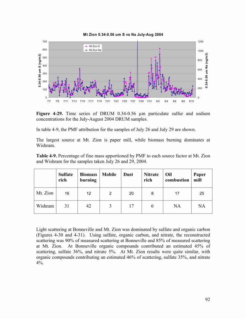
92
Mt Zion 0.34-0.56 um S vs Na July-Aug 2004
0
100
200
300
400
500
600
700
7/7 7/9 7/11 7/13 7/15 7/17 7/19 7/21 7/23 7/25 7/27 7/29 7/31 8/2 8/4 8/6 8/8 8/10
0.34
-0.5
6 um
S (n
g/m
3)
0
200
400
600
800
1000
1200
0.34
-0.5
6 um
Na
(ng/
m3)
Mt Zion SMt Zion Na
Figure 4-29. Time series of DRUM 0.34-0.56 µm particulate sulfur and sodium concentrations for the July-August 2004 DRUM samples.
In table 4-9, the PMF attribution for the samples of July 26 and July 29 are shown.
The largest source at Mt. Zion is paper mill, while biomass burning dominates at Wishram.
Table 4-9. Percentage of fine mass apportioned by PMF to each source factor at Mt. Zion and Wishram for the samples taken July 26 and 29, 2004.
Sulfate rich
Biomass burning
Mobile Dust Nitrate rich
Oil combustion
Paper mill
Mt. Zion 16 12 2 20 8 17 25
Wishram 31 42 3 17 6 NA NA
Light scattering at Bonneville and Mt. Zion was dominated by sulfate and organic carbon (Figures 4-30 and 4-31). Using sulfate, organic carbon, and nitrate, the reconstructed scattering was 90% of measured scattering at Bonneville and 85% of measured scattering at Mt. Zion. At Bonneville organic compounds contributed an estimated 45% of scattering, sulfate 36%, and nitrate 5%. At Mt. Zion results were quite similar, with organic compounds contributing an estimated 46% of scattering, sulfate 35%, and nitrate 4%.

93
Bonneville measured and reconstructed bsp July episode
0
10
20
30
40
50
60
70
80
7/20/04 7/21/04 7/22/04 7/23/04 7/24/04 7/25/04 7/26/04 7/27/04 7/28/04 7/29/04 7/30/04 7/31/04 8/1/04
Bsca
t (M
m-1
)
Bonne nephrec SO4 bsRec OC bsBonne Recon bsRec NO3 bs
Figure 4-30. Time series of measured and reconstructed scattering and scattering by major components at Bonneville during the July 2004 episode. Reconstructed light scattering is computed for sulfate, nitrate, and organic carbon compounds only.
Mt Zion measured and reconstructed bsp July 2004 episode
-10
0
10
20
30
40
50
60
70
80
7/20 7/21 7/22 7/23 7/24 7/25 7/26 7/27 7/28 7/29 7/30 7/31 8/1
Bsc
at (M
m-1
)
Mt Zion nephrec SO4 bsRec OC bsBonne Recon bsRec NO3 bs
Figure 4-31. Time series of measured and reconstructed scattering and scattering by major components at Mt. Zion during the July 2004 episode. Reconstructed light scattering is computed for sulfate, nitrate, and organic carbon compounds only.
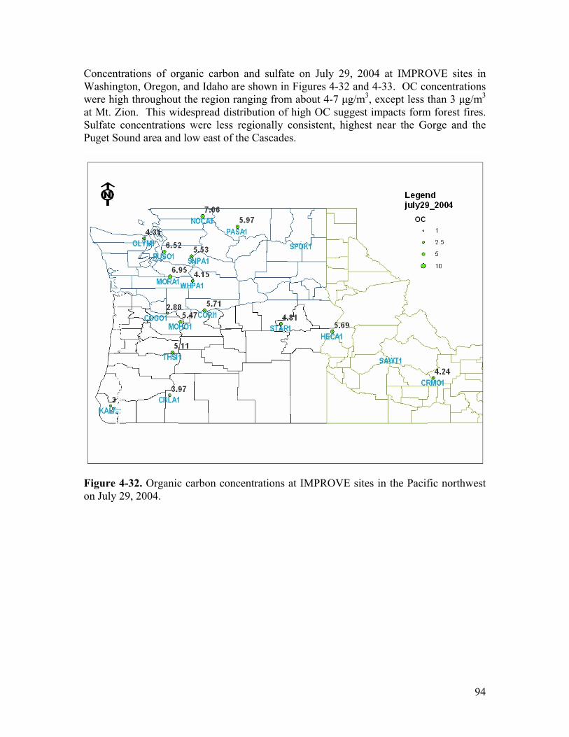
94
Concentrations of organic carbon and sulfate on July 29, 2004 at IMPROVE sites in Washington, Oregon, and Idaho are shown in Figures 4-32 and 4-33. OC concentrations were high throughout the region ranging from about 4-7 µg/m3, except less than 3 µg/m3 at Mt. Zion. This widespread distribution of high OC suggest impacts form forest fires. Sulfate concentrations were less regionally consistent, highest near the Gorge and the Puget Sound area and low east of the Cascades.
Figure 4-32. Organic carbon concentrations at IMPROVE sites in the Pacific northwest on July 29, 2004.
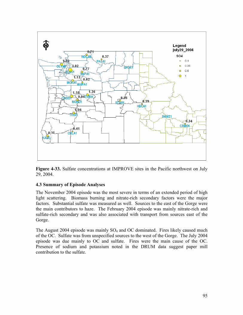
95
Figure 4-33. Sulfate concentrations at IMPROVE sites in the Pacific northwest on July 29, 2004.
4.3 Summary of Episode Analyses The November 2004 episode was the most severe in terms of an extended period of high light scattering. Biomass burning and nitrate-rich secondary factors were the major factors. Substantial sulfate was measured as well. Sources to the east of the Gorge were the main contributors to haze. The February 2004 episode was mainly nitrate-rich and sulfate-rich secondary and was also associated with transport from sources east of the Gorge.
The August 2004 episode was mainly SO4 and OC dominated. Fires likely caused much of the OC. Sulfate was from unspecified sources to the west of the Gorge. The July 2004 episode was due mainly to OC and sulfate. Fires were the main cause of the OC. Presence of sodium and potassium noted in the DRUM data suggest paper mill contribution to the sulfate.
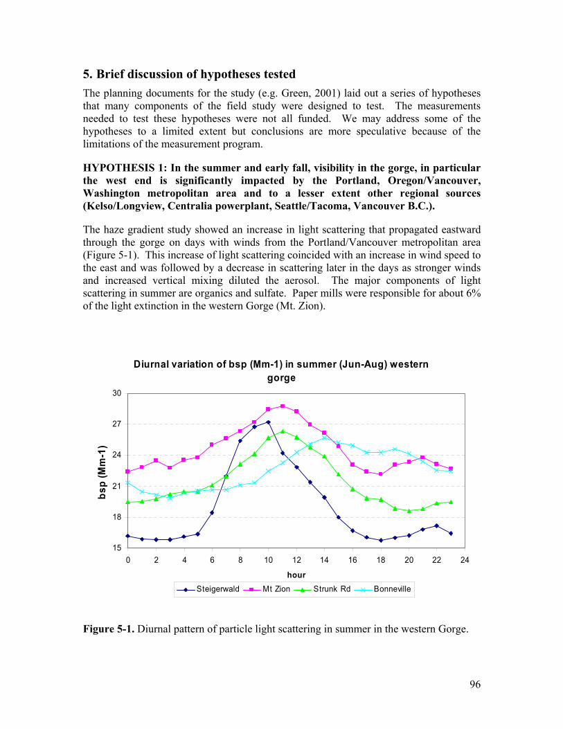
96
5. Brief discussion of hypotheses tested The planning documents for the study (e.g. Green, 2001) laid out a series of hypotheses that many components of the field study were designed to test. The measurements needed to test these hypotheses were not all funded. We may address some of the hypotheses to a limited extent but conclusions are more speculative because of the limitations of the measurement program.
HYPOTHESIS 1: In the summer and early fall, visibility in the gorge, in particular the west end is significantly impacted by the Portland, Oregon/Vancouver, Washington metropolitan area and to a lesser extent other regional sources (Kelso/Longview, Centralia powerplant, Seattle/Tacoma, Vancouver B.C.).
The haze gradient study showed an increase in light scattering that propagated eastward through the gorge on days with winds from the Portland/Vancouver metropolitan area (Figure 5-1). This increase of light scattering coincided with an increase in wind speed to the east and was followed by a decrease in scattering later in the days as stronger winds and increased vertical mixing diluted the aerosol. The major components of light scattering in summer are organics and sulfate. Paper mills were responsible for about 6% of the light extinction in the western Gorge (Mt. Zion).
Diurnal variation of bsp (Mm-1) in summer (Jun-Aug) western gorge
15
18
21
24
27
30
0 2 4 6 8 10 12 14 16 18 20 22 24
hour
bsp
(Mm
-1)
Steigerwald Mt Zion Strunk Rd Bonneville
Figure 5-1. Diurnal pattern of particle light scattering in summer in the western Gorge.
97
HYPOTHESIS 2: Visibility in the gorge, in particular, the east end is significantly impacted by urban and industrial sources in or near the gorge plus regional sources north and east of the gorge in the Columbia River basin in winter
The haze gradient study showed that the highest light scattering throughout the gorge occurs during easterly (downgorge) wind conditions. These conditions occur mainly in winter. The highest scattering is east of the Gorge at Towal Road and generally decreases through the Gorge to the west. This pattern suggests major impacts to visibility in the Gorge from sources to the east of the Gorge. The occurrence of nitrate and sulfate together in the nitrate-rich secondary PMF factor suggests a large source (e.g. Boardman power plant) may be largely responsible for this factor. This factor is greatest at Wishram and Mt. Zion with flow from the east. The biomass smoke factor is the second highest contributor to PM2.5 during the easterly flow days – this could be due to wood combustion in the Columbia River Basin cities and towns in winter. It was also noted that for downgorge flow an increase in light scattering occurs from Wishram (upgorge from the Dalles) to Memaloose and Sevenmile Hill (downgorge of the Dalles). Also, when the wind shifts from westerly to easterly the scattering at Sevenmile Hill increases. These findings suggest impacts of local sources in or near The Dalles. It should be noted that this increase is a small fraction of the total light scattering.
HYPOTHESIS 3: SO2 and NOX emissions from the Boardman coal-fired power plant just east and south of the gorge interact with ammonia from adjacent feed lots, in the presence of frequent low clouds and fog in winter to produce significant quantities of ammonium sulfate and ammonium nitrate that then moves into the gorge under drainage and larger scale pressure gradient flows.
As noted above, the PMF and wind pattern analysis suggest that the Boardman power plant is contributing significantly to sulfate and nitrate in the Gorge during winter.
HYPOTHESIS 4: Sources within the gorge are only minor contributors to aerosol and haze in the gorge.
As noted above, the haze gradient study indicated that sources within the Gorge did contribute to scattering in the Gorge. This was noted for easterly flow or periods with diurnally varying flow direction. The increase due to sources within the Gorge appeared to be a small fraction of overall light scattering.
HYPOTHESIS 5: Smoke from wildfires, prescribed fires, agricultural burning, and home heating occasionally causes significant visibility degradation in the gorge and surrounding areas.
The PMF analysis attributed 15% of the light extinction at both Wishram and Mt. Zion to smoke. The smoke factor was important both in winter and summer to fall, suggesting contributions from all the sources listed in the hypothesis.
98
6. Brief answers to Causes of Haze in the Gorge Questions In the contract for the Causes of Haze in the Gorge analysis, a series of questions were listed that were to be addressed. Many of these questions are addressed in sections of this report and the Haze Gradient Study report. However, for convenience they are briefly addressed here as well.
6.1 What aerosol components are responsible for haze?
6.1.1 What are the major components for best, worst, and average days and how do they compare? At Wishram, during the best and average days, sulfate is the major component contributing to aerosol light extinction, with a contribution of ~30% on both best and average days. OMC is the second largest contributor, with a contribution of ~20%. During the worst days, nitrate is the largest contributor to aerosol light extinction, with a contribution of 38%. Sulfate and OMC contribute 26% and 20%, respectively.
At Mt. Zion, during the best and average days, sulfate is the major component contributing to aerosol light extinction, with a contribution of ~30% on both best and average days. Nitrate and OMC each contributes about 20%. During the worst days, nitrate is the largest contributor to aerosol light extinction, with a contribution of 35%. Sulfate and OMC each contributes ~26%.
6.1.2 How variable were the major components episodically, seasonally, inter-annually, spatially? No statistically significant multi-year trends are found in Wishram for major components except sulfate which showed a significant decreasing trend during 1994-2004. Seasonally, nitrate is the largest contributor to aerosol light extinction in the first and fourth quarter, and sulfate is the largest contributor in the second and third quarter, each with a contribution of ~35-40%.
In Mt. Zion, because only 3 years of aerosol data are available, no multi-year trend can be analyzed. Seasonally, similar as at Wishram, nitrate is the largest contributor to aerosol light extinction in the first and fourth quarter, and sulfate is the largest contributor in the second and third quarter, each also with a contribution of ~35-40%.
Similar aerosol speciation is found at Mt. Zion (west side of the gorge) and Wishram (east side) except that there are more dusts (CM and fine soil) at Wishram especially during the second and third quarter of the year.
6.1.3 How do the relative concentrations of the major components compare with the relative emission rates nearby and regionally? This question is not straightforward to answer for the following reasons:
Good emissions inventories are not available for organic and elemental carbon and soil and coarse mass emissions. Sulfate and nitrate which contribute substantially to haze are

99
secondary pollutants and their formation is highly variable depending upon temperature, cloud cover, etc.
6.2 What is meteorology’s role in the causes of haze? The relationship between meteorological conditions and haze levels was addressed extensively in the Haze Gradient Study Report. They are summarized here.
6.2.1 How do meteorological conditions differ for best, worst and typical haze conditions? The best haze conditions were typically associated with summertime strong upgorge flow. These conditions led to particularly good visibility in the eastern Gorge. Days with precipitation were also associated with less haze than days without precipitation. Worst haze days were typically associated with winter downgorge flow. Under these conditions winds are light in the eastern Gorge and then increase in speed from the east in the western Gorge. Periods with regional wildland fires were also associated with high haze conditions. Meteorological conditions of hot, dry weather with lightning would thus be associated with forest fires and the resulting haze.
6.2.2 What empirical relationships are there between meteorological conditions and haziness? The along-gorge wind component was associated with haziness. Precipitation was associated with decreased haziness.
6.2.3 How does the spatial difference in meteorology and climate between west and east Scenic Area account for the haze differences observed between west and east Scenic Area? For the main summer wind pattern (strong upgorge), light scattering by particles (bsp) is about twice in the western Gorge as in the eastern gorge. While some of this is due to closer proximity to upwind major sources/source areas in the western Gorge, the eastern Gorge has much greater dispersion than the western Gorge due to stronger winds and deeper mixing. For winter downgorge, winds and dispersion are light in the eastern gorge and winds and therefore, alongwind dispersion is greater in the western gorge. Bsp for this pattern is significantly higher in the eastern Gorge than the western Gorge.
6.2.4 How well can haze conditions be predicted solely using meteorological factors? There were statistically significant differences in the haze levels for the five wind pattern types. However, there was substantial variability within each type as well.
6.2.5 How well can inter-annual variations in haze be accounted for by variations in meteorological conditions? The study period lasted for less than two years so the relationship between inter-annual variations in haze and meteorology was not addressed.

100
6.3 What are the emission sources responsible for haze?
6.3.1 What geographic areas are associated with transported air that arrives at sites on best, typical and worst haze days? Worst haze days are associated with wintertime transport from areas east of the gorge. Best haze days, particularly in the eastern gorge, were associated with strong flow from the west.
6.3.2 Are the emission characteristics of the transport areas consistent with the aerosol components responsible for haze? Yes. Worst haze periods with wintertime transport from the east has significant sources of NOX, ammonia, SO2 as well as organic mass from residential wood burning. Good and average day haze is dominated by sulfate and organic mass and transport from the west to east. There are significant sources of SO2 and sulfate to the west (e.g. power production, pulp and paper mills, shipping). Significant organic sources include mobile sources in the Portland urban area, wildfires and agricultural burning,
6.3.3 What do the aerosol characteristics on best, typical and worst days indicate about the sources? See the answer to the previous question.
6.3.4 What does the spatial and temporal pattern analysis indicate about the locations and time periods associated with sources responsible for haze? Sources east of the gorge mainly contribute to haze in winter. Sources west of the gorge contribute all year, contributing essentially every day in summer (but usually at lower levels of haze). Sources within the gorge contribute most noticeably during periods of flow reversal in the gorge (typically autumn).
6.3.5 What evidence is there for urban impacts on haze and what is the magnitude and frequency when evident? During summertime when winds are essentially always from the west, diurnal patterns in light scattering at the western and central gorge sites showed a “slug” of hazy air moving eastward through the gorge. This illustrates impacts from the Portland/Vancouver metropolitan area. For the most frequent summertime wind pattern (strong upgorge), daily average bsp increased from 14.8 mm-1 at Sauvie Island, upwind of the urban area to 22.7 Mm-1 at Mt. Zion, downwind of the cities. This represents about a 50% increase in particle light scattering across the urban area.
6.3.6 What connections can be made between sample periods with unusual species concentrations and activity of highly sporadic sources (e.g., major fires and dust storms, point source activity changes such as aluminum plant shut-downs, etc.)? The July 2004 and August 2004 episodes considered in the episode analysis section occurred during periods of major wildfires in the Pacific Northwest.

101
6.3.7 What can be inferred about impacts from sources in other regions? Forest fires outside of the Columbia River Gorge area contribute to haze in the region. Background levels of haze coming into the region and the source regions of this haze was not thoroughly investigated. Sites at the edges of the study region (e.g. Steigerwald to the west and Towal Road to the east) give some idea about outside source areas and background. Winds from the east and highest haze at the eastern sites during winter downgorge conditions implied impacts from source areas to the east of the gorge.
6.4 Are there detectable and/or statistically significant multi-year trends in the causes of haze?
6.4.1 Are the aerosol components responsible for haze changing? Because only 3 years of aerosol data are available at Mt. Zion, no trends analysis can be done for this site. At Wishram, 8 years of data (as shown in the table below) are available (based on Regional Haze Rule) for trends analysis. The trends analyses using the Theil method shows no statistically significant trends (i.e. P-Value <0.05) in total light extinction and light extinction due to major aerosol components except sulfate which was significantly deceased during 1994-2004.
Table 6-1. Data available at Wishram.
site Year aerosol_bext ammSO4f_bext ammNO3f_bext OMCf_bext ECf_bext SOILf_bext OMCf_bextCORI1 1994 46.98 14.57 10.24 10.83 4.47 0.66 10.83CORI1 1995CORI1 1996 41.3 12.43 9.35 9.58 4.13 0.55 9.58CORI1 1997 41.55 14.36 7.6 9.25 3.78 0.54 9.25CORI1 1998 39.25 12.84 5.4 10.09 4.66 0.83 10.09CORI1 1999 35.65 11.76 4.7 8.92 4.13 0.79 8.92CORI1 2000CORI1 2001 51.67 13.93 20.16 7.76 2.99 0.86 7.76CORI1 2002CORI1 2003 43.35 11.52 14.18 10.19 3.3 0.6 10.19CORI1 2004 49.12 11.48 16.74 10.57 3.55 0.78 10.57Slope 0.271 -0.225 0.67 -0.049 -0.117 0.011 -0.049P-Value 0.2742 0.0156 0.2742 0.4524 0.0894 0.1994 0.4524
6.4.2 Where aerosol component changes are seen, are they the result of meteorological or emissions changes? The only statistically significant trend was for sulfate at Wishram. Regional SO2 emissions have decreased since 1999 as controls were installed at the Centralia Powerplant in 2001 and 2002 and some aluminum smelter and pulp and paper mills ceased operation.
6.4.3 Where emissions are known to have changed, are there corresponding changes in haze levels? (e.g., aluminum plant shutdowns or emission controls on the Centralia Power Plant)? No. From the table above, decreases in sulfate scattering at Wishram due to regional decreases in SO2 emissions appears to have been offset by increases in nitrate scattering. However the increases in total aerosol light extinction and nitrate scattering were not statistically significant.
102
7. Conceptual Model for Haze in the Columbia River Gorge
7.1 Meteorological relationship to transport of pollutants and haze levels Winds through the Columbia River Gorge are driven by pressure gradients across the gorge, blowing from high to low pressure. Significant sources near or within the gorge that affect visibility include a variety of sources in the Portland/Vancouver metropolitan area to the immediate west of the gorge, additional industrial sources west of the gorge, small cities and mobile sources (ships, trains, trucks, and automobiles) within the gorge, electricity generation, dairy operations, and small urban areas (e.g. Tri-Cities) upriver from the gorge.
During summer winds are nearly always from west to east (upriver or upgorge). This is in response to a coast to interior pressure gradient that develops from heating of the interior compared to coastal areas and higher pressure offshore due to the location of the Pacific High. Winds increase in speed during the day as the pressure gradient increases due to increased temperature gradients. These winds transport pollutants from the Portland/Vancouver metropolitan area and industrial sources west of the gorge eastward through the gorge. In the western and central gorge, haze (light scattering) increases in late morning as winds transport these urban/industrial caused aerosols deeper into the gorge. At the eastern gorge sites, there is less haze due to the increased vertical and along-wind dispersion of these aerosols as they travel through the gorge.
The main summer meteorological pattern with strong upgorge flow has the lowest level of haze, with highest levels at the western gorge sites nearest the Portland urban area and lowest haze levels at the eastern sites.
In winter there is typically higher pressure east of the gorge and lower to the west. This results from cold stable air to the east and the prevalence of Pacific low pressure systems to the west. Under the most common winter pattern (winter downgorge), winds are light from the east in the eastern gorge and increase in speed as the air travels westward through the gorge. Haze levels are highest east of the gorge and gradually decrease to the west. Thus sources to the east of the gorge (e.g. Boardman power plant, nearby dairy operation, and the Tri-Cities areas) are major contributors to haze-causing aerosols that are transported through the gorge from east to west. This pattern has the highest haze levels of the main meteorological patterns. Nitrate, sulfate, and organic aerosols are the main contributors to haze. The contrast in haze levels between the haziest (winter downgorge) and least hazy (strong upgorge) wind patterns is much greater in the eastern gorge than in the western gorge.
During spring and fall pressure gradients are generally weaker and flows tend to be frequently lighter and may change direction diurnally. Under these conditions aerosols can slosh back and forth within the gorge and sources within the gorge become relatively more important as transport is reduced. Some effect of The Dalles on haze was noted for the flow reversal conditions.
During late summer, the most common meteorological condition has moderately strong west to east winds that have a large increase in speed during the day.
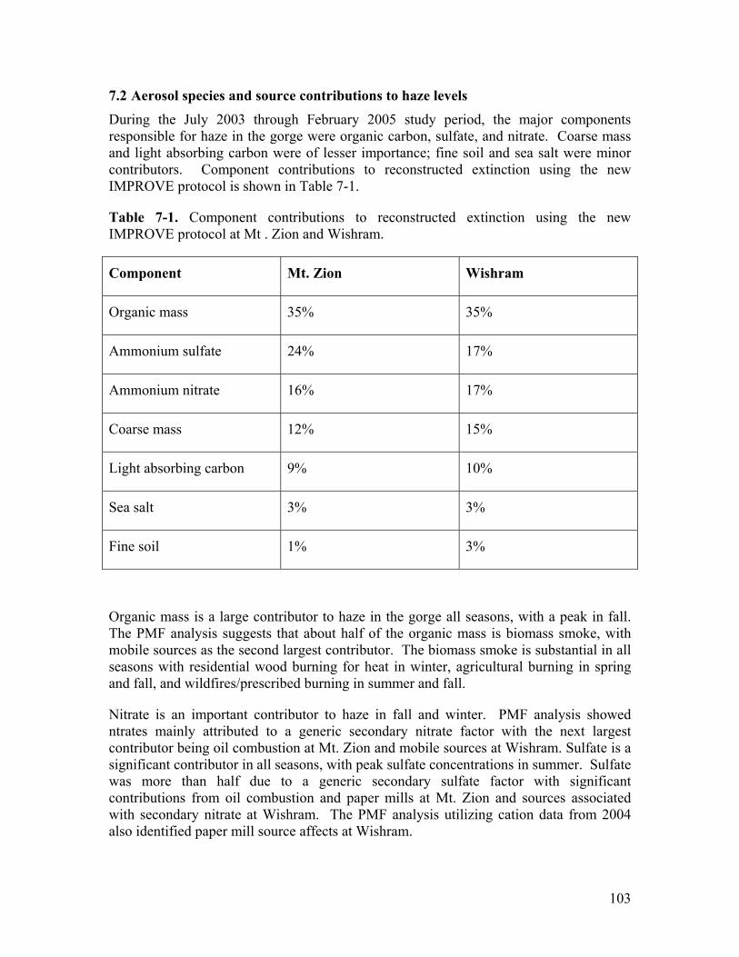
103
7.2 Aerosol species and source contributions to haze levels During the July 2003 through February 2005 study period, the major components responsible for haze in the gorge were organic carbon, sulfate, and nitrate. Coarse mass and light absorbing carbon were of lesser importance; fine soil and sea salt were minor contributors. Component contributions to reconstructed extinction using the new IMPROVE protocol is shown in Table 7-1.
Table 7-1. Component contributions to reconstructed extinction using the new IMPROVE protocol at Mt . Zion and Wishram.
Component Mt. Zion Wishram
Organic mass 35% 35%
Ammonium sulfate 24% 17%
Ammonium nitrate 16% 17%
Coarse mass 12% 15%
Light absorbing carbon 9% 10%
Sea salt 3% 3%
Fine soil 1% 3%
Organic mass is a large contributor to haze in the gorge all seasons, with a peak in fall. The PMF analysis suggests that about half of the organic mass is biomass smoke, with mobile sources as the second largest contributor. The biomass smoke is substantial in all seasons with residential wood burning for heat in winter, agricultural burning in spring and fall, and wildfires/prescribed burning in summer and fall.
Nitrate is an important contributor to haze in fall and winter. PMF analysis showed ntrates mainly attributed to a generic secondary nitrate factor with the next largest contributor being oil combustion at Mt. Zion and mobile sources at Wishram. Sulfate is a significant contributor in all seasons, with peak sulfate concentrations in summer. Sulfate was more than half due to a generic secondary sulfate factor with significant contributions from oil combustion and paper mills at Mt. Zion and sources associated with secondary nitrate at Wishram. The PMF analysis utilizing cation data from 2004 also identified paper mill source affects at Wishram.

104
An unresolved issue is how well the PMF analysis accounts for mobile sources. Mobile sources may contribute in part to the secondary nitrate and oil combustion factors. The occurrence of a higher source attribution to mobile emissions at Mt. Zion compared to Wishram suggests that the effect of mobile emission impact at Mt. Zion may be underestimated by PMF.
Biomass smoke and secondary nitrate are the most important source factors for the most common winter pattern (winter downgorge). At Mt. Zion, paper mill and oil combustion impacts were associated with winds from the west (upgorge), consistent with locations of these emissions sources.
105
8. References Allen, G.A.; Lawrence, J.; and Koutrakis, P. (1999). "Field validation of a semi-
continuous method for aerosol black carbon (aethalometer) and temporal patterns of summertime hourly black carbon measurements in southwestern Pennsylvania", Atmospheric Environment 33, 817~823.
Bench, G., Grant, P., Ueda, D., Cliff, S., Perry, K., Cahill, T. (2002). The Use of STIM and PESA to Measure Profiles of Aerosol Mass and Hydrogen Content, Respectively, across Mylar Rotating Drum Impactor Samples, Aerosol Sci. and Tech. 36: 642–651.
Birch, M.E.; and Cary, R.A. (1996). "Elemental Carbon-Based Method for Monitoring Occupational Exposures to Particulate Diesel Exhaust." Aerosol Science and Technology 25, 221-241.
Chow, J.C., Watson, J.G., Crow, D., Lowenthal, D.H., and Merrifield, T. (2001). Comparison of IMPROVE and NIOSH Carbon Measurements, Aerosol, Sci. Technol, 34, 23-34.
Chow, J.C., Watson, J.G., Chen, L.-W. A., Arnott, W.P., Moosmuller, H., (2004). Equivalence of elemental carbon by thermal/optical reflectance and transmittance with different temperature protocols. Environ. Sci. Technol., 38, 4414-4422.
Draxler, R. R. and G. D. Hess, Description of the Hysplit_4 modeling system. Report No. NOAA Tech Memo ERL ARL-224, December 1997. Prepared by Air Resources Laboratory, NOAA, Silver Spring, MD, 1997.
Green, M.; Arnott, P.; Walker, J.; and Etyemezian, V., 2003. Comparison of IMPROVE and NIOSH methods for elemental carbon aerosol measurements with a photoacoustic method in a wintertime urban desert environment. Abstracts of the 2003 European Aerosol Conference, J. Aer. Sci., 34, s1149-s1150.
Green, M., (2001). COLUMBIA RIVER GORGE VISIBILITY AND AIR QUALITY STUDY, Working Draft: Existing Knowledge and Additional Recommended Scientific Assessment to Consider. Prepared for Robert Bachman, US Forest Service, Portland, Oregon.
Interagency Monitoring of Protected Visual Environments (IMPROVE) – Data resources. National Park Service, Ft. Collins, CO. http://vista.cira.colostate.edu/improve, 2004.
Kim, E., P. K. Hopke, and E. S. Edgerton, Source identification of Atlanta aerosol by positive matrix factorization, J. Air & Waste Manage. Assoc., 53:731-739, 2003.
Knochel, Basic Principles of XRF with Synchrotron Radiation, 2nd International Workshop on XRF and PIXE Applications in Life Science, Capri, Italy, 29-30 June, 1989, World Scientific Publishing Co., Singapore, 1990.

106
Lind, T., Hokkinen, J., Jokiniemi, J., Hillaino, R., Makkonen, U., Raukola, A., Rintanen, J., Saviharju, K., 2006. Electrostatic precipitator performance and trace element emissions from two Kraft recovery boilers. ES&T, 40, 584-589.
Liu, W, P. K. Hopke, and R. A. VanCuren, Origins of fine aerosol mass in the western United States using positive matrix factorization, J. Geophys. Res., 108, D23, 4716, doi:10.1029/2003JD003678, 2003.
Lundgren, D. A., An Aerosol Sampler for Determination of Particle Concentration as a Function of Size and Time, J. Air Poll. Cont. Assoc. 17, 225-229 (1967).
Malm, W.C., J.F. Sisler, D. Huffman, R.A. Eldred, and T.A. Cahill. Spatial and seasonal trends in particle concentration and optical extinction in the United States. Journal of Geophysical Research, VOL. 99, No. D1, 1347-1370, 1994.
Malm, W. C., B. A. Schichtel, M. L. Pitchford, L. L. Ashbaugh, and R. A. Eldred, Spatial and monthly trends in speciated fine particle concentration in the United States, J. Geophys. Res., 109, D03306, doi:10.1029/2003JD003739, 2004.
Molenar, J. “Theorectical and Experimental Analysis of the Optec NGN nephelometer”. http://vista.cira.colostate.edu/improve/Publications/GrayLit/gray_literature.htm accessed February 2006.
Moosmuller, H. (1998). "Photoacoustic and filter measurements related to aerosol light absorption during the Northern Front Range Air Quality Study (Colorado 1996/1997)", JGR, 103, issue D21, 28149-28157.
Raabe,O.G., Braaten, D.A., Axelbaum, R.L., Teague,S.V., Cahill, T.A. “Calibration studies of the DRUM impactor”, J. Aerosol Sci., 1988,19,183.
Visibility Information Exchange Web System (VIEWS) Database. Cooperative Institute for Research in the Atmosphere (CIRA), Colorado State University, Ft. Collins, CO. http://vista.cira.colostate.edu/views/, 2004.
Watson, J.G., Visibility: Science and regulation. J. Air & Waste Management Assoc., 52(6):628-713, 2002.
Watson, J. G., 1979. Chemical element balance receptor model methodology for assessing the sources and fine and total suspended particulate matter in Portland, Oregon. Doctoral dissertation, Oregon Graduate Center, February 1979.