Cash Flow Risk Management in the Property/Liability ... · Industry: A Dynamic Factor Modeling...
34
Cash-Flow Risk Management in the Insurance Industry: A Dynamic Factor Modeling Approach Sponsored by Society of Actuaries’ Committee on Finance Research Prepared by Patricia Born Hong-Jen Lin Min-Ming Wen * November 2014 © 2014 Society of Actuaries, All Rights Reserved The opinions expressed and conclusions reached by the authors are their own and do not represent any official position or opinion of the Society of Actuaries or its members. The Society of Actuaries makes no representation or warranty to the accuracy of the information. * Patricia Born is a Professor in the Department of Risk Management & Insurance, Real Estate and Legal Studies, Florida State University. Hong-Jen Lin is an Assistant Professor in the Department of Finance & Business Management, The City University of New York. Min-Ming Wen is an Assistant Professor in the Department of Finance & Law, California State University, Los Angeles. All comments can be addressed to Min-Ming Wen via e- mail: [email protected]. We gratefully acknowledge the financial support provided by the Society of Actuaries’ Committee on Finance Research. We are grateful to the reviewers, Steven Craighead, Steven Siegel, and Barbara Scott for their helpful comments and persistent support.
Transcript of Cash Flow Risk Management in the Property/Liability ... · Industry: A Dynamic Factor Modeling...

Cash-Flow Risk Management in the Insurance
Industry: A Dynamic Factor Modeling Approach
Sponsored by
Society of Actuaries’
Committee on Finance Research
Prepared by
Patricia Born
Hong-Jen Lin
Min-Ming Wen *
November 2014
© 2014 Society of Actuaries, All Rights Reserved
The opinions expressed and conclusions reached by the authors are their own and do not represent any official position or opinion
of the Society of Actuaries or its members. The Society of Actuaries makes no representation or warranty to the accuracy of the
information.
* Patricia Born is a Professor in the Department of Risk Management & Insurance, Real Estate and Legal Studies,
Florida State University. Hong-Jen Lin is an Assistant Professor in the Department of Finance & Business
Management, The City University of New York. Min-Ming Wen is an Assistant Professor in the Department of
Finance & Law, California State University, Los Angeles. All comments can be addressed to Min-Ming Wen via e-
mail: [email protected].
We gratefully acknowledge the financial support provided by the Society of Actuaries’ Committee on Finance
Research. We are grateful to the reviewers, Steven Craighead, Steven Siegel, and Barbara Scott for their helpful
comments and persistent support.

© 2014 Society of Actuaries, All Rights Reserved Page 2
Introduction
This project models cash-flow risks and empirically analyzes cash-flow risk management of
insurance firms under a dynamic factor modeling framework, which can capture the dynamic
interactions between an insurance firm’s activities in financing, investing, underwriting, and risk
transferring. In addition, through the use of a factor-augmented autoregressive (FAAR)
technique, the empirical analysis can simultaneously consider the effects of macro-factors that
are common to the entire economy as well as those factors specific to the insurance industry.
Cash is king. It is true for entrepreneurs, and it is also true for managers of financial
institutions. Cash-flow risks have long been one of the most essential factors while managing a
variety of risks, particularly for the insurance industry, which faces unique underwriting risks not
observed in other industries. To the insurance industry, cash flows can be generated through
underwriting activities, financing and investing choices, and even managing risks; consequently
modeling cash-flow risks will be on a dynamic basis process because it is essential to forecasting
and managing financial and underwriting risks.
To model the cash-flow risks specific to the insurance industry, we have to capture the
dynamics of the cash-flow–generating process of an insurer. The cash-flow–generating process
can be characterized by two major components: (1) the earnings that result from core activities
and cannot be modified and (2) other profits that can be modified through the dimensions of
investment choices, risk management, and financial policies. In addition, the factors underlying
the cash-flow–generating process may be intertwined and thus under the generating process can
present the risks to the extent of cash-flow level. For instance, the downside risk of a company
can be signaled by an abnormal decrease in operating cash flows. Moreover, the discrepancy of
the magnitude and timing of the cash flows generated from underwriting insurance policies and

© 2014 Society of Actuaries, All Rights Reserved Page 3
those generated from investment activities create cash-flow uncertainty and risks to insurance
firms.
For insurance firms, cash flows generated from investment, underwriting, and risk
management activities are important indicators in financial management and are the key
variables in capital budgeting decisions. Hence, these generated cash flows will provide
internally interacting feedback on determining the insurers’ strategies of underwriting, risk
management, and investment from time to time. Correspondingly, cash-flow processes and cash-
flow risks demonstrate their dynamic characteristics.
This study investigates management of cash flows by the insurance industry by
incorporating its interactions with risk management and investment management after
identifying and capturing the dynamic relationships between one another. For example, an
efficient implementation of a risk management mechanism can mitigate agency costs deriving
from overinvestments of free cash flows. In addition, a well-established investment portfolio can
efficiently utilize free cash flows for better asset allocation. Furthermore, we extend the research
to explicitly consider the dynamic effects of economy-wide macro-variables and industry-wide
common factors. The research sample, based on the insurance industry, provides an opportunity
to incorporate the factors uniquely specific to this industry, namely, insurance underwriting
cycles and regulatory requirements, into the model. Therefore, this study conducts a
comprehensive analysis of cash-flow modeling and cash-flow risk management in the insurance
industry.
The existing literature provides evidence that suggests the relationships between cash
flows, investment, and risk management. As demonstrated in Alti (2003), cash flows contain
valuable information about a firm’s investment opportunities. In addition, Almeida et al. (2004)

© 2014 Society of Actuaries, All Rights Reserved Page 4
identify the significant relationship between cash-flow sensitivity and financial constraints.
Rochet and Villeneuve (2011) examine how risk management mechanisms interact with the
uncertainty of cash-flow levels and conclude that the decisions are simultaneously endogenous.
In addition, the literature has shown that insurers have more actively participated in the
derivative markets by employing financial derivatives not only to smooth cash-flow uncertainty
from their invested assets and underwriting liabilities but also to generate more cash flows.
Therefore, cash-flow management is important in the field of risk management, particularly for
the insurer firms who intend to reach effective asset/liability duration management. To the best
of our knowledge, very few of the existing studies have addressed the issues of cash-flow risk
management of insurers under the framework of considering the dynamic risk management in
investing, financing, and underwriting.
In this project we apply dynamic factor modeling (Stock and Watson 2006, 2009) to
capture the dynamic interactions between risk management and investment management by
incorporating economy-wide macro-variables and industry-wide business cycle variables.
Moreover, to further empirically carry out the applications of dynamic factor modeling as
suggested in Rochet and Villeneuve (2011), we utilize a factor-augmented autoregression model
(FAARM) through which we model how cash flows respond to the dynamic interactions
mentioned above to explicitly model the nonmonotonic effects. The research by Born et al.
(2009) and Lin et al. (2011) explores the dynamic interactions between risk management and
financial management in the U.S. property and liability insurance industry, but the explicit
effects on cash-flow management are left for future research in their study. As financial
intermediaries, the insurance industry is subject to various sources of risk, including interest rate
risk, market risk, credit risk, and liquidity risk. Engaging in investment activities is one major

© 2014 Society of Actuaries, All Rights Reserved Page 5
source that generates the risks mentioned above, and the variability of cash flows reflects a
firm’s risks (Keown et al. 2007; Shin and Stulz 2000). All risks, particularly liquidity risk, are
related to cash flows. Bakshi and Chen (2007) concluded that investing in stocks leads to the
cash flows embedded with higher risks. Ballotta and Haberman (2009) and Azcue and Muler
(2009) specifically examine the investment strategies of insurance companies and emphasize
minimizing the default risks of the insurers, but not the dynamic optimal investment strategies of
insurers over economic downturns. In other words, they estimate the credit risk or liquidity risk
at the firm level but fail to consider the macroeconomic issues such as interest risk and market
risk. The study by Wen and Born (2005) explores the dynamic interactions between investment
strategies and underwriting cycles, and their study suggests that although one may investigate
how insurers dynamically adjust their investment and hedging strategies, the dynamic
interactions between asset and liability risks corresponding to the underwriting cycles should be
taken into consideration.1
Taken with these earlier studies, our study intends to bridge the extant literature by taking
steps further to model the cash-flow risks by taking into account the uncertainty of the market
cycles, thereby explicitly examining insurers’ cash-flow management. Using the highly regulated
insurance industry as a research sample enables us to further extend the existing literature by
incorporating the specific industry-wide characteristics, such as regulatory requirements and
underwriting cycles, in the models. The simultaneous consideration of market cycle,
underwriting cycle, and regulatory requirements enables us to fully depict the insurance firms’
investment, risk management, and underwriting strategies.
1 As suggested by Fairley (1979), expected earnings to be realized at the end of a policy year consist of the
underwriting profit margin and investment returns; this highlights the importance of considering the interactions
between investment and underwriting activities.

© 2014 Society of Actuaries, All Rights Reserved Page 6
This study, by taking into account the different phases of market cycles, provides a
thorough examination of insurers’ investment and hedging strategies in each phase (e.g., market
upturn or downturn) of a cycle from the stage of including conventional investments to the stage
of including the innovative financial derivatives as investment and hedging tools. Thus, we will
draw a conclusion on how the inclusion of hybrid assets (for hedging and investment) can
expand insurers’ investment portfolios and in addition can dynamically adjust insurers’
investment strategies as they face market downturns. Through the application of dynamic
financial modeling (DFM), the dynamic adjustment between investment, underwriting, and
hedging strategies corresponding to different phases of cycles (market cycle and underwriting
cycle) can be captured.
Methods
Cash-Flow–Generating Process
Based on Rochet and Villeneuve (2011), we modify the cash-flow–generating process dCt for an
insurer, which can be characterized as
dCt = (µdt + σdWt) + rtCtdt + (σRdWRt − LdPt ) − dZt + (dIt − dVt), (1)
where (µdt + σdWt) corresponds to the underwriting profits of an insurance firm: µ is the
expected profitability per unit of time, σ is the volatility of ‘‘primary’’ earnings, and Wt a
standard Wiener process, which cannot be hedged or insured. We use rt as the rate of return
generated from investment through asset allocation or from derivative use for income generation;
hence, rtCtdt is the investment cash inflows. Here (σRdWRt − LdPt ) corresponds to the risks that
can be managed through the use of either financial derivatives or reinsurance. Zt is the

© 2014 Society of Actuaries, All Rights Reserved Page 7
(nondecreasing) cumulative payout process, It is the additional funds accumulated through
financing by issuing securities, and Vt is the corresponding financing costs.
The cash-flow–generating process shown in equation (1) demonstrates that for an
insurance firm, cash-flow management involves underwriting, investing, financing, and risk-
transferring management. Nevertheless, it is not easy to estimate equation (1) in practice since
the empirical model should contain more variables than those in equation (1). Henceforth, we
extend the dynamic factor modeling by following Almeida et al. (2004) to dynamically estimate
the cash flows’ sensitivity to financial constraints. The DFM considered in this study is a
dimension-reduction technique that incorporates more information in the calculation and thus is
able to depict the dynamic patterns of cash flows of an insurance company.
Dynamic Factor Modeling
Dynamic factor modeling (DFM) is being more frequently applied by policymakers and
economic researchers for forecasting purposes by considering the key macroeconomic variables.
To the best of our knowledge, this project is the first study to apply DFM in the insurance
industry to describe firm-level cash-flow volatility with the consideration of macro-variables and
factors uniquely specific to the insurance industry, namely, regulatory requirements and
underwriting cycles. Stock and Watson (2002), Forni et al. (2005), and Kapetanios and
Marcellino (2004) conclude that DFM can be applied to extract common factors. From the
model, all or a subset of the estimated factors can be empirically carried out through the
utilization of regression models for prediction purposes.
Specifically, DFM was developed by Geweke (1977) and further revised by Giannone et
al. (2004) and Watson (2004). Although DFM is an extension of factor analysis, it can depict a
© 2014 Society of Actuaries, All Rights Reserved Page 8
time-varying nature by considering the dynamic patterns of factor analysis. As a result, we are
able to apply DFM to incorporate macro-common factors (such as underwriting cycles specific
to the insurance industry and macroeconomic variables to all industries) as well as firm-specific
features in modeling cash flows. In addition, the application of DFM can solve the
multicolinearity problem when too many variables are considered in a regression function (see
Sargent and Sims 1977, among others). Moreover, as we incorporate macro-business cycles and
underwriting cycles in the analysis, it is likely to observe structural changes along with the
presence of cycles. The application of DFM enables us to explicitly depict the structural changes
embedded in business cycles while theoretically modeling the factors and empirically analyzing
the data (Sargent and Sims 1977; Belviso and Milani 2006).
Stock and Watson (2005) propose the factor forecasting model, in which the factors are
constructed by using predictors in the following dynamic structural equation:
ttt eFX (2)
where tX contains observable variables,
tF is the estimated unobservable latent factors,
is the factor-loading matrix, and te is the error term. In other words, X can be explained by F
through the estimation of factor loadings. In particular, tF includes both firm- and industry-level
factors. The firm-level factors contain the latent variables related to insurers’ activities in
underwriting, investing, and derivatives usage, and the industry-level factors include the latent
variables related to the macro-variables as well as industry-specific variables, namely, regulatory
requirements and underwriting cycles. The dynamic interactions are captured through the factor
loading and are therefore reflected intX ; they explicitly describe the observed derivative
usage, investment asset allocation, and insurance underwriting. In sum, based on dynamic factor
modeling, the dynamic interactions between derivatives utilization, investment asset allocation,
N

© 2014 Society of Actuaries, All Rights Reserved Page 9
and underwriting are captured in equation (2) by incorporating macro- as well as firm-specific
variables. The DFM model applied in this study distinguishes itself from previous literature by
the fact that the model does not require strong assumptions on the objective function, such as
firm value maximization or total cost minimization, which are discussed in the literature
associated with cost or profit efficiency (Cummins et al. 1999; Cummins and Weiss 2000;
Cummins and Xie 2008).
Integrating a cash-flow–generating process into the dynamic cash-flow model, a FAARM
can be developed as an equation by considering not only cross-sectional characteristics, but also
time-series factors. In light of Almeida et al. (2004), we apply the model in equation (3) to depict
how cash flows are shown after the aforementioned interactions are simultaneously taken into
consideration:
1 '
1 1α γ Φ( ) ,t t t tC F L C u (3)
where 1
1tC is the one-period forecast cash flow at time t, tF is the estimated unobservable
factors from equation (2),tCL)( is the lagged cash flows at time t, and
1tu is the random error for
the estimated dependent variables. This model can be further carried out for empirical
applications. Based on the model setup, we extend this functional process to a measurable system
that can capture the dynamic interactions and draw an equilibrium/optimal status for risk
management investment and underwriting strategies. The estimation results TF̂ from equation (2)
along with equation (3) enable us to derive the empirical autoregression model (FAARM)
described in equation (4):
TTT
FAAR
TT CLFC )(ˆˆˆˆˆ '1,
|1 . (4)

© 2014 Society of Actuaries, All Rights Reserved Page 10
Data
To carry out the applications of dynamic factor modeling for an explicit and comprehensive
examination of insurers’ cash-flow management, this study conducts an empirical analysis by
employing the data pertaining to derivative transactions and the data related to insurers’
underwriting, investment, and financing activities. In particular, we gathered data through access
to a subscribed insurance database of SNL Financial that provides statutory financial data for the
property and liability insurance industry. Through the utilization of SNLxl, we chose the data
from prebuilt insurance templates, such as assets, liabilities, investment portfolios, cash flows,
income statements, and derivatives transactions (Schedule DB). We collected quarterly data over
the period 2001–2012 to ensure the feasibility of a time-series model with sufficient observations
over periods.
In particular, the data collected are to identify insurers’ underwriting, investing, and
financing. In addition, the variations of cash flows as well as firm characteristics are retrieved.
Furthermore, to incorporate the macro-factors into analysis, we include the macro-variables
pertaining to economic growth, interest rate, inflation rate, and unemployment rate. We retrieved
these macro-variables from Economic Research & Data, compiled by the Federal Reserve
Board.2 We require an insurer with nonnegative assets and premiums written in each quarter to
be included in the sample. The data collection gives us a total of 1,275 firms to perform the
dynamic factor model including the firm-level variables and macroeconomic variables that
capture economic cycles.
2 http://www.federalreserve.gov/econresdata/default.htm.

© 2014 Society of Actuaries, All Rights Reserved Page 11
This sample enables us to conduct principal components analysis and apply a dynamic factor
time-series model for each of the 1,275 firms over the 48-quarter time period to make induction
through the empirical results.
For brevity, in the following sections, we first use one randomly selected firm to conduct
the analyses and employ the results from this firm to illustrate the feasibility and applicability of
the models. Furthermore, we conduct subgroup analyses by categorizing the entire sample of
1,275 firms based on firm size into three subsamples: large-firm, medium-firm, and small-firm
groups. Empirical results from the entire group and subgroup analyses enable us to infer the
feasibility of applying DFM proposed in this study in forecasting cash flows and thus managing
cash-flow risks in the insurance industry. 3
Variable Construction
To empirically carry out the applications of FAARMs to manage cash flows through forecasting,
we utilize equation (2) as the first step to identify the main principal components: the latent
variables denoted by Ft through the observed variables, Xt. The second step is to incorporate the
variables depicting the principal components identified through significance comparison from
the first step’s analysis to predict future cash flows. In particular, through the principal
component analysis, which explains the cash-flow variables related to underwriting, investing,
financing, and risk-managing activities, the generated principal components are culled as the
main factors and are incorporated in equation (4) along with an autoregression model to forecast
the cash flows of the next period. Cash flow (CF) is the main variable involved in each step of
3 The dynamic factor models developed can be empirically applied to the insurance industry of life or property-
liability (P-L). At this stage, with the limit of data access, the current study utilizes the data collected from the P-L
insurance companies to demonstrate the effectiveness of DFM empirical applications.

© 2014 Society of Actuaries, All Rights Reserved Page 12
model application and estimation. To infer comparable results among firms, we construct a
normalized CF variable, ln(CFi,t – min(CFi,t)). It is constructed by taking the logarithm of the
difference of the cash flows of firm i at time t (CFi,t) and the minimal cash flow among all
observations (min(CFi,t)).4
The time-series model estimation calls for the unit root test to infer an appropriate order for
an autoregression model (AR), and the results suggest a first-order autoregression model, AR(1),
that is more appropriate based on the principle of root mean square error (RMSE) minimization.
The application of a dynamic factor model is carried out by incorporating this AR(1) model
along with the principal components derived from step (1), namely, AR(1) + ∑ 𝑃𝐶𝑗𝑘=1 k , in
which the optimal number of principal components (PC) can also be determined through the
minimization of the RMSE of the model.
In terms of the choice of those observed variables Xt in equation (2), we follow the analysis
of Born et al. (2009) and categorize the variables mainly pertaining to (1) capital management,
(2) investment and financial management, and (3) risk management. In addition, we choose the
variables capturing insurers’ firm characteristics and their underwriting activities as well as the
macroeconomic environment. The variables in each category depict different risk factors of an
insurance firm. Table 1 summarizes the variables under study in the first step (equation [2]) of an
FAARM.
4 We follow the conventional method applied in the study of the profit frontier to normalize the key variable.

© 2014 Society of Actuaries, All Rights Reserved Page 13
Table 1 Definitions of the Variables Utilized in the Model
Capital Management Variables
Cap_AT Capital/surplus to asset ratio
Leverage Ratio of liability to total assets
Firm Characteristics Variables
Size Natural logarithm of the total assets
IT_R Ratio of computer and equipment (quarterly report: electronic data
processing equipment and software)
Investment (Financial) Management Variables
Bd_R Bond investment to total assets ratio
PStk_R Preferred stock to total assets ratio
CStk_R Common stock to total assets ratio
Mtg_loan_R Mortgage loans on real estate to total assets
RealE_R Real estate to total assets ratio
Sterm_R Short-term investment to total assets ratio
LTerm_R Long-term investment to total assets ratio
Risk Management Variables
Deri_R Ratio of derivatives to total assets
ReInsAsset_R Ratio of reinsurance premium written to total premium written
Underwriting Activities Variables
NetPremRec_R Net premium ratio
UW_R1 Underwriting gain (loss) to total assets ratio
NPW_GPW Ratio of net premium written to gross premium written
Macroeconomic Variables
Growth Economic growth rate based on U.S. GDP
Interest rate 10-year Treasury bond yield
Unemployment U.S. unemployment rate
Inflation Inflation rate based on U.S. CPI
Empirical Results
In the empirical analyses, for each individual insurance firm, we have conducted a time-series
analysis for the 48 quarters for the period 2001–2012. Consequently we come up with time-
series results for 1,275 firms with feasible data. It is essential to find means to better categorize
these sample firms based on common features. In this study, we use firm size as a basis to

© 2014 Society of Actuaries, All Rights Reserved Page 14
categorize firms into different groups and conduct the analyses for (1) the entire group, (2) a
large-firm group, (3) a medium-firm group, and (4) a small-firm group. To better illustrate the
procedures of applying the model, we base our study on a randomly selected firm to present the
results of each step of the DFM application. The results provide us with evidence supporting the
accessibility and applicability of the DFM model for its forecasting power of cash flows.
Principal Components Results
The time series analysis incorporating equations (2) and (3) is carried out in this section. We
illustrate the empirical results of the principal component analysis with a selected typical firm,
C1. The results are shown in Table 2. Since the model is performed based on a standardized data
set, the value of the estimated coefficient for each variable describes how much that variable
contributes to the principal component. In Table 2 we indicate the coefficients that are larger
than 0.20 (Franklin et al. 1995) with an asterisk sign to indicate its comparative significance to
other variables and investigate the patterns of each principal component.
As shown in Table 2, principal component 1 (PC1) is more related to the variables in the
categories of capital, investment, and risk managements through the magnitudes of the
corresponding coefficients. For example, the capital ratio variable (Cap_AT) has a coefficient
0.2797, whereas the preferred-stock (PStk_R), real estate investment (RealE_R), and the risk
management variable of the derivative ratio (Deri_R) all have a larger coefficient, 0.3280, than
the others.
For principal component 2 (PC2), it can be depicted by the following significant
variables: capital ratio (Cap_AT), IT ratio (IT_R), short-term investment ratio (STerm_R), and
reinsurance ratio (ReInsAsset_R). In other words, PC2 pertains to insurers’ capital management,

© 2014 Society of Actuaries, All Rights Reserved Page 15
investment management, risk management, and underwriting activities. In addition, among the
macro-variables, interest rate and unemployment rate present significant but contrasting effects
illustrating PC2. On the other hand, for principal component 3 (PC3), the variables pertaining to
the insurer’s underwriting activities and investment management are more significant to describe
PC3. In particular, underwriting gain (UW_R1) has a significant coefficient with value 0.4279,
whereas the net premium ratio (NPW_GPW) shows a negative and significant coefficient,
−0.3210. In addition for the investment activities, the investment in common stocks (CStk_R) is
significant with a coefficient magnitude of 0.4753. Moreover, for principal component 4 (PC4),
all three underwriting variables—net premium to assets ratio, underwriting gains, and net
premium to gross premium written ratio—are significant and negatively associated with PC4.
Consequently, among the associations between the principal components and insurers’
cash-flow management,5 PC1 and PC2 are more relevant to capital, investment, and risk
management, whereas PC3 and PC4 are relevant to investment management. In addition, PC2,
PC3, and PC4 all pertain to underwriting activities, whereas PC4 presents a more significant
association compared to PC2 and PC3.
To carry out the empirical application of DFM modeling, we first identify how a
principal component can be associated with those observed variables in the categories of insurers
in capital management, investment management, risk management, underwriting activities, and
macro-factors. The results of a significant relation between principal components and observed
proxy variables have demonstrated the feasibility of the measured model. For the next step in
5 We utilize the number of significant variables in each category of cash-flow management to infer the
corresponding association between principal components and proxy variables. For example, in the category of
investment management, for PC1 and PC2, there are three significant variables. On the other hand, for PC3 and
PC4, two of the variables are significant in this category.

© 2014 Society of Actuaries, All Rights Reserved Page 16
applying DFM modeling, we incorporate the results from principal component analysis into
autoregression cash-flow forecasting models (FAARMs) to further demonstrate the forecasting
power of this model. Taken as a whole, this model enables insurers to forecast cash flow for the
next time period and therefore further manage cash-flow risks.

© 2014 Society of Actuaries, All Rights Reserved Page 17
Table 2
Empirical Result of Principal Component Analysis
PC1 PC2 PC3 PC4
Capital management
Cap_AT 0.2797a 0.2427a -0.0538 0.1723
Leverage −0.2797a −0.2427a 0.0538 −0.1723
Firm characteristics
Size
−0.3383a 0.0506 −0.0498 0.0018
IT_R −0.1317 −0.4256a −0.2105a 0.0874
Investment (financial)
management
Bd_R 0.2279a 0.2741a −0.2920a 0.1225
PStk_R 0.3280a −0.0706 0.0601 −0.1451
CStk_R −0.1474 −0.1072 0.4753a 0.3106a
RealE_R 0.3280a −0.0706 0.0601 −0.1451
Sterm_R 0.0059 −0.3387a −0.1094 −0.2444a
LTerm_R 0.2574a −0.2161a 0.1609 −0.1550
Risk management
Deri_R 0.3280a −0.0706 0.0601 −0.1451
ReInsAsset_R −0.1932 −0.3205a −0.0133 −0.1981a
Underwriting activities
NetPremRec_R −0.1832 0.2626a 0.1990 −0.3449a
UW_R1 0.1112 0.0321 0.4279a −0.2505a
NPW_GPW −0.0217 −0.0075 −0.3210a −0.5514a
Macroeconomic variables
Growth 0.0246 −0.1168 0.4770a 0.0251
Interest rate 0.1544 −0.3486a −0.1283 0.2812a Unemployment −0.1801 0.3498a 0.0712 −0.2099a
Inflation 0.0297 −0.0197 0.0945 -0.0688
Note: Utilizing principal component analysis is the first step to carry out the application of DFM modeling through
the combination of equations (2) and (3):
ttt eFX , (2)
where tX contains observable variables.
tF is the estimated unobservable latent factors, is the factor
loading matrix, and te is the error term:
1
1 1α γ Φ( ) ,t t t tC F L C u (3)
where 1
1tC is the one-period forecast cash flow at time t, tF is the estimated unobservable factors from equation
(2), tCL)( is the lagged cash flows at time t, and
1tu is the random error for the estimated dependent variables.
aThe magnitude of the coefficient is larger than 0.20. See Table 1 for the definition of each variable.
N

© 2014 Society of Actuaries, All Rights Reserved Page 18
Table 3
Empirical Results of FAAR (DFM) of Firm C1
AR(1) FAAR1
FAAR2
FAAR3
FAAR4
FAAR5
AR(1) AR(1) + PC1 AR(1) + ∑ 𝑃𝐶2𝑗=1 j
AR(1) + ∑ 𝑃𝐶3𝑗=1 j
AR(1) + ∑ 𝑃𝐶4𝑗=1 j
AR(1) + ∑ 𝑃𝐶5𝑗=1 j
Coefficient t value Coefficient t value Coefficient t value Coefficient t value Coefficient t value Coefficient t value
Constant 2.74552 3.77*** 2.84106 3.89*** 4.56867 5.11*** 4.56316 5.02*** 4.92116 5.62*** 4.92096 5.55***
lnCF(t−1) 0.54789 4.56*** 0.53216 4.42*** 0.24766 1.68* 0.24857 1.66 0.18962 1.32 0.18965 1.30
PC1 0.00005 1.18 0.00006 1.50 0.00006 1.48 0.00006 1.58 0.00006 1.56
PC2 0.00021 2.94*** 0.00021 2.89*** 0.00024 3.32*** 0.00024 3.28***
PC3 −0.00001 −0.06 0.00000 −0.02 0.00000 −0.02
PC4 −0.00020 −2.38** −0.00020 −2.35**
PC5 0.00000 0.01
R2 0.3163 0.3372 0.4481 0.4482 0.5151 0.5151
RMSE 0.00079 0.00078 0.00072 0.00073 0.00069 0.00070
R2 changea 6.61% 32.89% 0.02% 14.93% 0.00%
RMSE changeb −1.27% −7.69% 1.39% −5.48% 1.45%
Note: This is the second step in carrying out the application of the FAARM through equation (4):
TTT
FAAR
TT CLFC )(ˆˆˆˆˆ '1,
|1 , (4)
where the estimation results TF̂ are obtained from equations (2) and (3) in the first step.
a R2 change is defined as the percentage of the R2 increase as one more principal component is included in AR; i.e., {R2[AR(1) + ∑ 𝑃𝐶𝑘+1𝑗=1 j)] – R2[AR(1) +
∑ 𝑃𝐶𝑘𝑗=1 j]}/{R2[AR(1) + ∑ 𝑃𝐶𝑘
𝑗=1 j]}. b RMSE change is defined as the percentage of RMSE decrease as one more principal component is included in AR; i.e., {RMSE[AR(1) + ∑ 𝑃𝐶𝑘+1
𝑗=1 j)] –
RMSE[AR(1) + ∑ 𝑃𝐶𝑘𝑗=1 j]}/{RMSE[AR(1) + ∑ 𝑃𝐶𝑘
𝑗=1 j]}. ***, **, and * denote the significance at the 1 percent, 5 percent, and 10 percent levels, respectively.

© 2014 Society of Actuaries, All Rights Reserved Page 19
Illustrations of FAAR (DFM) Applications
To empirically demonstrate the applications of DFM, we first use one selected sample firm to
illustrate the second step of utilizing a different number of principal components into
autoregression to infer DFM and evaluate its forecasting power. Tables 3 and 4 summarize the
results based on that single selected firm. Following similar procedures, we apply DFM to the
entire sample of 1,275 firms and the subgroups of entire the sample categorized by firm size.6
Table 3 shows the empirical results of FAARMs incorporating a different number of
principal components derived from step 1 through the autogression model, namely, AR(1) +
∑ 𝑃𝐶𝑘𝑗=1 j, where k is an optimum number of principal components to be determined via
comparison of root mean square error (RMSE). Mathematically, the more PCs that are involved
in the model, the higher the R2 is expected to be, and the more acute forecasting the model can
accomplish. Nevertheless, although the inclusion of an additional principal component may
significantly increase the model’s accuracy, it is not necessary to increase the number of PCs
included in the model. We implement five FAARMs, namely, FAAR 1: AR1 + one principal
component, FAAR 2: AR1 + two principal components, … , FAAR 5: AR1 + five principal
components.
In addition, as indicated in Table 3, among the five FAARMs, the models including the
second PC (PC2) and the fourth PC (PC4) consistently show their significance (at least at the 5
6 For each individual firm in the entire sample, we conduct the same analyses as described in Tables 2 and 3. It is
unnecessary to present all the results for all 1,275 sample firms. The results presented are based on a summary of the
analyses for all 1,275 firms.

© 2014 Society of Actuaries, All Rights Reserved Page 20
percent level).7 Referring to the first step of FAARM as shown in Table 2, the second PC is
featured by its significant relation with capital management through the opposite relations with
capital ratio and leverage, with investment risk through bond investment (Bd_R) and short-term
and long-term investment (Sterm_R, Lterm_R), and with risk management through reinsurance,
underwriting activities, and macroeconomic risk (interest rate and unemployment rate). On the
other hand, the fourth PC (PC4) tends to be linked to all the proxy variables representing
underwriting activities: NetPremRec_R, UW_R1, and NPW_GPW. PC4 also links to investment
management through common stock (CStk_R) and short-term investment (Sterm_R), to risk
management through reinsurance utilization, and to macroeconomic risk (interest rate and
unemployment rate).
In particular, the time-varying movements of the second and the fourth PCs are depicted
in Figure 1, which shows the cyclical characteristics. The approximate long-run paths of both
PCs decrease after year 2001 and bounce back after 2008. This pattern shows that these two PCs
are related to the macroeconomic risk, which decreases first and then increases, which coincided
with the overall trend of risk in the environment of all the financial markets. We conjecture that
the decrease in risk after 2001 may be caused by the adoption of the Sarbanes-Oxley Act, and the
increasing pattern after 2008 signals the advent of the subprime mortgage crisis. The small
variation of the second PC may represent the investment cycle. The variation for the fourth PC
may indicate the insurance underwriting cycle due to the fact that the underwriting variables
(NetPremRec_R, UW_R1, NPW_GPW) are more significant and important factors in the
composition of the fourth PC. In Figure 1, the macroeconomic variables demonstrate the biggest
7 As shown in Table 3, adding PC5 is insignificant in the estimation, and therefore it is not reported in Table 2 to
save space.

© 2014 Society of Actuaries, All Rights Reserved Page 21
waves, going downward after 2001 and then upward during and after 2009, whereas the
underwriting variables may represent a smaller cycle around the patterns of macroeconomic
variables.
Figure 1
Cyclical Patterns of Principal Components of the Sample Firm
Note: PC 2 is the estimated second principal component, and PC4 is the fourth principal component of the sample
firm. They are the only two significant principal components out of five.
Table 3 also shows the R2 and RMSE for each model and the relative changes from
including one additional principal component. As shown in the table, RMSE of the model
decreases from 0.00078 to 0.00072 when the model increases the number of principal
components from one to two with the relative change of 7.69 percent. In addition, the inclusion
of PC2 shows significance at the 1 percent level with the coefficient of 0.00021. The model

© 2014 Society of Actuaries, All Rights Reserved Page 22
shows another significant increase in R2 and a decrease in RMSE as the model includes four PCs
compared to three PCs. Moreover, in the AR(1) + ∑ 𝑃𝐶4𝑗=1 j model, PC2 and PC4 both show
significant effects on forecasting the next period cash flow. Although the model increases the
number of principal components from four to five, no decrease in RMSE or significant increase
is observed in R2. As a result, for this sample firm, we conclude that the FAARM with four
principal components can best forecast the cash flows for the next period.
Table 4 illustrates the steps of empirically applying the DFM model to forecast the cash
flows for the fourth quarter of 2012 by using the observed variables in the third quarter of 2012.
In addition, Table 4 demonstrates the forecasting power of this DFM model. Panel A reports the
actual observed value for each variable defined in Step 1 (listed in Tables 1 and 2). Based on the
results of principal component analysis, Panel B summarizes the estimated value of each
principal component by incorporating the estimated coefficients derived from Step 1 (shown in
Table 2). For the FAARM including four components along with the first order of the
autoregression model, that is, AR(1) + ∑ 𝑃𝐶4𝑗=1 j as shown in Table 3, the forecast cash flows of
the fourth quarter of 2012 along with the actual value of cash flows are reported in Panel C. As
demonstrated, the absolute value of the forecasting error is about 0.000003 in the logarithm term,
or equivalent to $0.13 per thousand dollars of cash flow.
In sum, for this one sample firm, the empirical results from the applications of DFM
provide evidence supporting the feasibility and applicability of the model. In addition, the model
provides relatively strong forecasting power to estimate future cash flows.

© 2014 Society of Actuaries, All Rights Reserved Page 23
Table 4
Forecasting Values of FAAR Model
Panel A: Observed Values
2012Q3
Panel B: Cash Flows of
2012Q3 and Estimated PC
Panel C: Observed and
Forecast Cash Flow
Observed
Value
Cap_AT 0.3965
lnCF(t−1) 6.073528 Observed lnCF
2012Q4
6.073244
Size 5.5925
𝑃𝐶1̂ −2.9970 Forecast lnCF
2012 fourth
quarter
6.073545
IT_R 0.0004 𝑃𝐶2̂ 2.3686 Difference ($) 0.130436
Bd_R 0.5787 𝑃𝐶3̂ 0.0363
PStk_R 0.0030 𝑃𝐶4̂ −1.7100
CStk_R 0.2401
Mtg_loan_R 0.0000026
RealE_R 0.0000077
Sterm_R 0.0000026
LTerm_R 0.0000026
Deri_R 0.0000026
ReInsAsset_R 0.0561
NetPremRec_R 0.0013
UW_R1 −0.0063
NPW_GPW 1.1867
Leverage 0.6035
Growth 0.7676
Interest rate 1.7200
Unemployment 7.8000
Inflation 0.4462
Empirical Results of FAAR (DFM) for the Entire Sample
For each firm of the entire sample, we examine the baseline of autoregression (AR) model as
well as the optimum number of principal components to be included in the AR model through
the comparison of RMSE. It is not necessary to present the results for each of the 1,275 different

© 2014 Society of Actuaries, All Rights Reserved Page 24
firms.8 In addition, because the coefficients of PCs may vary from firm to firm and the empirical
results of FAAR may differ from firm to firm, we categorize these 1,275 sample insurers based
on their firm size to make an induction for grouping. Through categorization, insurers can
correspondingly conduct their cash-flow forecasting and management based on common models
fitted to the specific category. In particular, based on the amount of total assets of each firm, we
sort these 1,275 firms by a descending order and classify them by asset level as (1) large firms,
(2) medium firms, and (3) small firms. Such a grouping results in a similar number of
observations in each group, 400, 400, and 475 firms in large, medium, and small firm groups,
respectively. The accomplishment of this categorizing analysis will contribute to the literature by
providing a more general cash-flow forecasting model to the insurance industry.
8 For each firm, two baseline models will be conducted, and the corresponding RMSE will be compared to
determine an appropriate baseline model included in the FAARM. This will produce 1275×2 RMSEs and 1275×2
R2. In the second step of performing the FAAR technique, the FAARM consists of the best baseline model along
with an optimum number of principal components. The optimum number (n) of principal components based on
RMSE will be determined by comparing the RMSE of at least (n−1) FAARMs with (n−1) principal components. As
a result, it will generate about 1,275×n RMSEs and 1,275×n R2.
© 2014 Society of Actuaries, All Rights Reserved Page 25
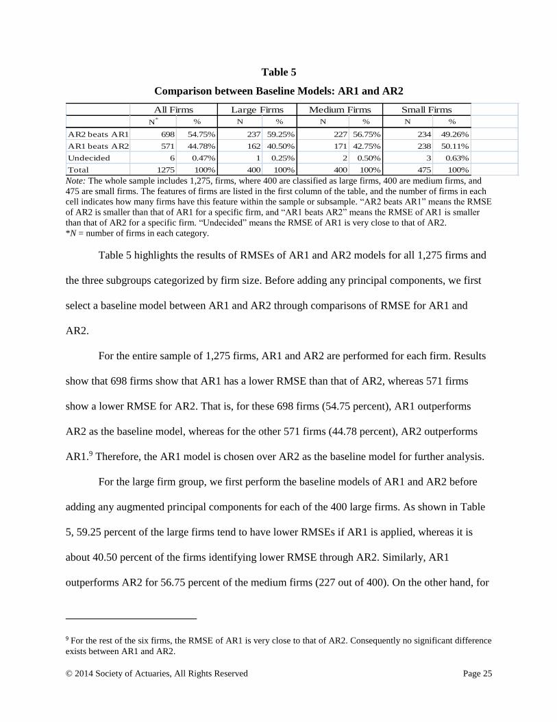
Table 5
Comparison between Baseline Models: AR1 and AR2
N* % N % N % N %
AR2 beats AR1 698 54.75% 237 59.25% 227 56.75% 234 49.26%
AR1 beats AR2 571 44.78% 162 40.50% 171 42.75% 238 50.11%
Undecided 6 0.47% 1 0.25% 2 0.50% 3 0.63%
Total 1275 100% 400 100% 400 100% 475 100%
All Firms Large Firms Medium Firms Small Firms
Note: The whole sample includes 1,275, firms, where 400 are classified as large firms, 400 are medium firms, and
475 are small firms. The features of firms are listed in the first column of the table, and the number of firms in each
cell indicates how many firms have this feature within the sample or subsample. “AR2 beats AR1” means the RMSE
of AR2 is smaller than that of AR1 for a specific firm, and “AR1 beats AR2” means the RMSE of AR1 is smaller
than that of AR2 for a specific firm. “Undecided” means the RMSE of AR1 is very close to that of AR2.
*N = number of firms in each category.
Table 5 highlights the results of RMSEs of AR1 and AR2 models for all 1,275 firms and
the three subgroups categorized by firm size. Before adding any principal components, we first
select a baseline model between AR1 and AR2 through comparisons of RMSE for AR1 and
AR2.
For the entire sample of 1,275 firms, AR1 and AR2 are performed for each firm. Results
show that 698 firms show that AR1 has a lower RMSE than that of AR2, whereas 571 firms
show a lower RMSE for AR2. That is, for these 698 firms (54.75 percent), AR1 outperforms
AR2 as the baseline model, whereas for the other 571 firms (44.78 percent), AR2 outperforms
AR1.9 Therefore, the AR1 model is chosen over AR2 as the baseline model for further analysis.
For the large firm group, we first perform the baseline models of AR1 and AR2 before
adding any augmented principal components for each of the 400 large firms. As shown in Table
5, 59.25 percent of the large firms tend to have lower RMSEs if AR1 is applied, whereas it is
about 40.50 percent of the firms identifying lower RMSE through AR2. Similarly, AR1
outperforms AR2 for 56.75 percent of the medium firms (227 out of 400). On the other hand, for
9 For the rest of the six firms, the RMSE of AR1 is very close to that of AR2. Consequently no significant difference
exists between AR1 and AR2.

© 2014 Society of Actuaries, All Rights Reserved Page 26
the small firm sample, 49.26 percent (234 out of 475) of the firms show that AR2 with lower
RMSEs is a better baseline model than AR1. As a result, we conclude that AR1 is an appropriate
baseline model to predict cash flows with higher accuracy for large-firm and medium-firm
subsamples. AR2 is an appropriate model for small firms.
Table 6
Results of FAARM: Number of Models That Outperform the Baseline Model
N*
% N % N % N %
5 models beatAR1 420 32.94% 112 28.00% 127 31.75% 181 38.11%
At least 4 models beat AR1 634 49.73% 190 47.50% 200 50.00% 244 51.37%
At least 3 models beat AR1 768 60.24% 227 56.75% 241 60.25% 300 63.16%
At least 2 models beat AR1 883 69.25% 278 69.50% 270 67.50% 335 70.53%
At least 1 model beats AR1 1130 88.63% 398 99.50% 365 91.25% 367 77.26%
No model beat AR1. 145 11.37% 2 0.50% 35 8.75% 108 22.74%
Total 1275 100.00% 400 100.00% 400 100.00% 475 100.00%
All Firms Large Firms Medium Firms Small Firms
Note: The whole sample includes 1,275 firms, where 400 are classified as large firms, 400 are medium firms, and 475
are small firms. The features of firms are listed in the first column of this table, and N indicates the number of firms
with the above feature listed in the first column. “5 models beats AR1” means the RMSE of any one of the five models
is smaller than that of the baseline AR1 model; “at least 4 models beat AR1” means the RMSEs of four to five models
are smaller than that of AR1; “at least 3 models beat AR1” means the RMSEs of three to five models are smaller than
that of AR1; “at least 2 models beat AR1” means the RMSEs of two to five models are smaller than that of AR1; and
“at least one models beat AR1” means the RMSE of only one out of the five models is smaller than that of AR1.
*N = number of firms in each category.
As the FAARM consists of a baseline model along with principal components, after
identifying AR1 as the baseline model, we next examine whether use of the FAARM can further
improve forecasting power compared to the baseline models in terms of the corresponding
RMSE. Without prespecifying the number of principal components added to the baseline model
to form the DFM model, Table 6 summarizes the RMSE of AR1 and different DFM models. In
particular, we identify the five DFM models by the number of principal components (PCs)
© 2014 Society of Actuaries, All Rights Reserved Page 27
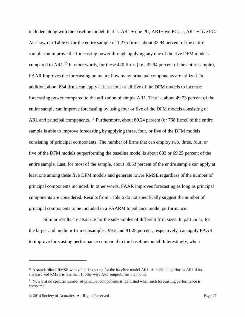
included along with the baseline model: that is, AR1 + one PC, AR1+two PC,…, AR1 + five PC.
As shown in Table 6, for the entire sample of 1,275 firms, about 32.94 percent of the entire
sample can improve the forecasting power through applying any one of the five DFM models
compared to AR1.10 In other words, for these 420 firms (i.e., 32.94 percent of the entire sample),
FAAR improves the forecasting no matter how many principal components are utilized. In
addition, about 634 firms can apply at least four or all five of the DFM models to increase
forecasting power compared to the utilization of simple AR1. That is, about 49.73 percent of the
entire sample can improve forecasting by using four or five of the DFM models consisting of
AR1 and principal components. 11 Furthermore, about 60.24 percent (or 768 firms) of the entire
sample is able to improve forecasting by applying three, four, or five of the DFM models
consisting of principal components. The number of firms that can employ two, three, four, or
five of the DFM models outperforming the baseline model is about 883 or 69.25 percent of the
entire sample. Last, for most of the sample, about 88.63 percent of the entire sample can apply at
least one among these five DFM models and generate lower RMSE regardless of the number of
principal components included. In other words, FAAR improves forecasting as long as principal
components are considered. Results from Table 6 do not specifically suggest the number of
principal components to be included in a FAARM to enhance model performance.
Similar results are also true for the subsamples of different firm sizes. In particular, for
the large- and medium-firm subsamples, 99.5 and 91.25 percent, respectively, can apply FAAR
to improve forecasting performance compared to the baseline model. Interestingly, when
10 A standardized RMSE with value 1 is set up for the baseline model AR1. A model outperforms AR1 if its
standardized RMSE is less than 1; otherwise AR1 outperforms the model.
11 Note that no specific number of principal components is identified when such forecasting performance is
compared.

© 2014 Society of Actuaries, All Rights Reserved Page 28
comparing results across different subsamples, we find that in the small-firm subsample, 38.11
percent of firms are featured with better FAARMs with any different number of principal
components. On the other hand, in the large-firm subsample, this number decreases to 28.00
percent. That is, the variation of cash flows in large firms is usually larger, and the quality of the
explanatory variables is better. Therefore, it is possible to use fewer principal components to
capture the variation of cash flows for large firms, whereas the models for small firms need more
principal components to explain the variation of the dependent variable (cash flows).
Overall, results from Table 6 suggest that a baseline model along with principal
components enables a FAARM to increase its forecasting accuracy. However, these results do
not specify the number of principal components to be included in the FAARMs that can further
reduce RMSE. Following the preliminary conclusions from one-sample results summarized in
Table 3, we implement five FAARMs: FAAR 1: AR1 + one principal component, FAAR 2: AR1
+ two principal components, … , FAAR 5: AR1 + five principal components; see Table 7. In
addition, the choice of the number of principal components can rely on the analysis of
eigenvalues.12
12 Untabulated results suggest that as five principal components are incorporated, more than 70 percent of the
variation of the cash flows of the same period is captured. Henceforth, it is not necessary to add more factors in the
FAAR approach.

© 2014 Society of Actuaries, All Rights Reserved Page 29
Table 7
Results of FAARM: Optimum Number of Principal Components
Model Best % Best % Best % Best %
FAAR1: (AR1+1PC) 174 13.65% 2 0.50% 32 8.00% 140 29.47%
FAAR2: (AR1+2PCs) 833 65.33% 397 99.25% 309 77.25% 127 26.74%
FAAR3: (AR1+3PCs) 165 12.94% 0 0.00% 30 7.50% 135 28.42%
FAAR 4: (AR1+4PCs) 184 14.43% 0 0.00% 21 5.25% 163 34.32%
FAAR5 (AR1+5PCs) 294 23.06% 0 0.00% 31 7.75% 263 55.37%
Total 1275 400 400 475
All Firms Large Firms Medium Firms Small Firms
Note: The number in each cell represents the number and percentage of firms with that best model. For example,
here 174 out of 1,275 firms are featured with FAAR1as the best model, which is 13.65 percent of the entire sample,
833 out of 1,275 firms (65.33 percent) are featured with FAAR2 as the best model, etc. Note that the summation of
the percentages is not 100 percent because more than one best model may exist for a specific firm.
To further identify the optimum number of principal components incorporated in a
FAARM, we conduct the five FAARMs for each firm. Results are summarized in Table 7, in
which the RMSE of each corresponding model within a firm is compared. Consequently, within
a firm, a best FAARM is identified by the minimum RMSE among the five FAARMs. In
particular, similar to step 2 in applying FAAR (DFM) to the selected firm shown in Table 3,
among all 1,275 firms, each model is performed for each of the 1,275 firms, and the
corresponding RMSE and R2 of each model can be obtained. After performing the five models
for each firm and ordering the RMSEj for firm I, RMSEi,j stands for the RMSE for firm i under
model j, where i is from firm 1 to firm 1,275 and j is from model 1 to model 5. For firm i, the
minimum of RMSE from model j can be identified.13
A forecasting DFM model is the combination of the baseline model AR1 and a different
number of principal components. The optimum number of principal components is determined
13 Note that the vertical summation of the number of firms in Table 7 is not 1,275 since there may be more than one
best model within a firm.

© 2014 Society of Actuaries, All Rights Reserved Page 30
by RMSE comparisons. We define FAAR1 as AR1 + one principal component, FAAR1 as AR1
+ two principal components, …, and FAAR5 as AR1 + five principal components.
Table 7 shows that the RMSE of FAAR1, …, FAAR5 for each firm demonstrates that the
inclusion of more principal components does not necessarily lower the corresponding RMSE.
For the entire sample, FAAR3 is the best model for about 12.94 percent of this sample, and
FAAR4 is the best for 14.43 percent of it. On the other hand, for the large-firm sample, neither
FAAR3, FAAR4, nor FAAR5 can serve as the best model. Nevertheless, FAAR3, FAAR4, and
FAAR5 are the best models for 7.50, 5.25, and 5.75 percent of the medium firms, respectively,
and they are also the best models for 28.42, 34.32, and 55.37 percent of the small firms,
respectively. It is worth noting that when the size of a firm is small, FAAR with more factors
tends to be the best model. Nevertheless, as the baseline model includes three, four, or five
principal components, they perform as the best models for more sample firms. For example,
about 294 (23.06 percent) firms of the entire sample can acquire the best forecast cash flows
through the application of FAAR5, that is, AR1 + five principal components. As we further
explore the forecasting power of the FAARMs across different categories of firms with different
sizes, for large and medium firms, FAAR2 (AR1+2PCs) is identified as the best forecasting
model with the respective 99.25 and 77.25 percent of firms with minimum RMSE, while for
small firms, the FAAR5 model (i.e., AR1 + five PCs) is found to be the best forecasting model
by which 55.37 percent of the firms are modeled and forecast with minimum RMSE.
Conclusions
This study applies a novel dynamic factor model (FAAR) to explain and forecast the time-
varying patterns of cash flows of U.S. insurance companies. A principal component approach is

© 2014 Society of Actuaries, All Rights Reserved Page 31
employed to capture the augmented factors to be utilized for forecasting. This forecasting model
incorporates risk management, capital management, the underwriting cycle, financial
(investment) management, and macroeconomic risk and provides a reduced-dimension
estimation. We first described the cash-flow–generating process and theoretical model of cash
flows and then measured the FAARM.
Results from the first step (principal component analysis) aid in determining the
macroeconomic cycles and underwriting cycles. The importance of derivatives investments and
stock investments can also be observed for each insurance firm. Results from the second step
offer evidence supporting that the dynamic factor model (or FAARM) improves the in-sample
forecasting by reducing RMSE. The incorporation of principal components can further decrease
RMSE for a majority of firms. Results are consistent for the entire sample as well as for different
subsamples. In addition, with expected stable cash flows, large firms tend to have better
forecasting by utilizing fewer principal components. As we observe, FAAR2 for large firms
dominantly outperforms (99.25 percent) all other models. This ratio decreases to 77.25 percent
for medium firms and 26.74 percent for small firms. FAAR5 is the best model for small firms.
Such results suggest that for smaller firms, it takes more principal components to explain the
variation of cash flows. We expect that the findings from this study can contribute to the practice
of forecasting cash flows. Since the firm size can be identified, the corresponding proposed DFM
to the firm size can be consequently applied by the insurer to forecast cash flows. In addition,
following the identification of the variation of cash flows from the forecasting models, an insurer
can further apply different financial instruments to control and manage the variation of cash
flows, that is, cash-flow risks.

© 2014 Society of Actuaries, All Rights Reserved Page 32
References
Almeida, H., M. Campello, and M. S. Weisbach. 2004. The Cash Flow Sensitivity of Cash.
Journal of Finance 59: 1777–1804.
Alti, A. 2003. How Sensitive Is Investment to Cash Flow When Financing Is Frictionless?
Journal of Finance 58: 707–722.
Azcue, P., and N. Muler. 2009. Optimal Investment Strategy to Minimize the Ruin Probability of
an Insurance Company under Borrowing Constraints. Insurance: Mathematics and
Economics 44: 26–34.
Bakshi, G., and Z. Chen. 2007. Cash Flow Risk, Discounting Risk, and the Equity Premium
Puzzle. In Handbook of Investments: Equity Premium, edited by Rajnish Mehra, 377-402.
Amsterdam: North Holland.
Ballotta, L., and S. Haberman. 2009. Investment Strategies and Risk Management for
Participating Life Insurance Contracts. Available at http://ssrn.com/abstract=1387682.
Belviso, F., and F. Milani. 2006. Structural Factor-Augmented VARs (SFAVARs) and the
Effects of Monetary Policy. B.E. Journal of Macroeconomics 6: 1-46.
Born, P., H.-J. Lin, M. Wen, and C. C. Yang. 2009. The Dynamic Interactions between Risk
Management, Capital Management, and Financial Management in the U.S.
Property/Liability Insurance Industry. Asia-Pacific Journal of Risk and Insurance 4: 2–
17.
Cummins, J. D., S. Tennyson, and M. A. Weiss. 1999. Consolidation and Efficiency in the U.S.
Life Insurance Industry. Journal of Banking & Finance 23: 325–357.
Cummins, J. D., and M. A. Weiss. 2000. Analyzing Firm Performance in the Insurance Industry
Using Frontier Efficiency and Productivity Methods. In Handbook of Insurance, ed.
Georges Dionne,767-829. Norwell, MA: Kluwer Academic Publishers.
Cummins, J. D., and X. Xie. 2008. Mergers and Acquisitions in the US Property-Liability
Insurance Industry: Productivity and Efficiency Effects. Journal of Banking & Finance
32: 30–55.
Fairley, W. 1979. Investment Income and Profit in Property-Liability Insurance: Theory and
Empirical Results. Bell Journal of Economics 10: 192–210.

© 2014 Society of Actuaries, All Rights Reserved Page 33
Forni, M., M. Hallin, M. Lippi, and L. Reichlin. 2005. The Generalised Dynamic Factor Model: One
Sided Estimation and Forecasting. ULB Institutional Repository 2013/10129. Université
Libre de Bruxelles.
Franklin, S. B., D. J. Gibson, P. A. Robertson, J. T. Pohlmann, and J. S. Fralish. 1995. Parallel
Analysis: A Method for Determining Significant Principal Components. Journal of
Vegetation Science 6: 99–106.
Geweke, J. 1977. The Dynamic Factor Analysis of Economic Time Series. In Latent Variables in
Socio-Economic Models, edited by Dennis J. Aigner and Arthur S. Goldberger, 365-383.
Amsterdam: North-Holland.
Giannone, D., L. Reichlin, and L. Sala. 2004. Monetary Policy in Real Time. NBER
Macroeconomics Annual 19:161–200.
Kapetanios, G., and M. Marcellino. 2004. A Comparison of Estimation Methods for Dynamic
Factor Models of Large Dimension. Queen Mary Working Paper No. 489.
Keown A. J., J. D. Martin, and J. W. Petty. 2007. Foundations of Finance: The Logic and
Practice of Financial Management. New York: Prentice Hall.
Lin, H. J., M. Wen, and C. C. Yang. 2011. Effects of Risk Management on Cost Efficiency and
Cost Function of the U.S. Property and Liability Insurers. North American Actuarial
Journal 15: 487–498.
Rochet, J.-C., and S. Villeneuve. 2011. Liquidity Management and Corporate Demand for
Hedging and Insurance. Journal of Financial Intermediation 20: 303–323.
Sargent, T. J., and C. A. Sims. 1977. Business Cycle Modeling without Pretending to Have Too
Much A-Priori Economic Theory. In New Methods in Business Cycle Research, edited by
C. Sims et al., 45-109. Minneapolis: Federal Reserve Bank of Minneapolis.
Shin, H., and R. M. Stulz. 2000. Shareholder Wealth and Firm Risk. Dice Center working paper
2000-19.
Stock, J. H., and M. W. Watson. 2002. Macroeconomic Forecasting Using Diffusion Indexes.
Journal of Business and Economic Statistics 20: 147–162.
Stock, J. H., and M. W. Watson. 2005. Implications of Dynamic Factor Models for VAR
Analysis. NBER Working Paper Series 11467: 1-65.
Stock, J. H., and M. W. Watson. 2006. Forecasting with Many Predictors. In Handbook of
Economic Forecasting, edited by G. Elliott, Clive W. J. Granger, and A. Timmermann,
pp. 515–554. Amsterdam: Elsevier.
© 2014 Society of Actuaries, All Rights Reserved Page 34
Stock, J. H., and M. W. Watson. 2009. Forecasting in Dynamic Factor Models Subject to
Structural Instability. In The Methodology and Practice of Econometrics: Festschrift in
Honor of D. F. Hendry, edited by N. Shephard and J. Castle, 1-57. Oxford: Oxford
University Press.
Watson, M.W. 2004. Comment on Giannone, Reichlin, and Sala. NBER Macroeconomics
Annual, 2004: 216–221.
Wen, M., and P. Born. 2005. Firm-Level Analysis of the Effects of Net Investment Income on
Underwriting Cycles: An Application of Simultaneous Equations. Journal of Insurance
Issues 28: 14–32.