CALCULATION OF TURBULENT SHEAR STRESS IN SUPERSONIC

BOUNDARY LAYER FLOWS

by

Chen-Chih Sun

and nP4

Morris E. Childs' o cUniversity of Washington, Seattle, Washington 0 >

W W

Turbulent shear stress distributions for supersonic boundary layer P. v Mto H L

flows have been computed from experimental mean boundary layer data. The o "

computations have been made by numerically integrating the time aver ged n

continuity and streamwise momentum equations. The computational method < C)*0 a

is different from those previously reported in that integrated mass and

momentum flux profiles and differentials of these integral quantities o0

Oare used in the computations so that local evaluation of the streamwise t I

flows upstream and downstream of shock wave-boundary layer interactions 0 )4 t

and for both two-dimensional and axisymmetric flows. The computed

results are compared with recently reported shear stress measurements

wh- .ch were obtained by hnot wire anemometer and laser -veo eterA.

niques. For most of the results shown reasonably good agreemer ,is'fou a

This work was supported by NASA Grant NGR-48-002-047 tder ad ,.a- N

tion of the Aerodynamics Branch, Ames Research Cente-r.

Index Categories: Boundary layers and convective heat tra sf ,l. v-Turbulent supersonic and hypersonic flow

" Shock waves

RIesearch Associate (Postdoctoral), Department of Mechanical En.gineer-ing, University of Washington, Seattle, Washington. Member AIAA.

+

Professor and Chairman, Department of Mechanical Engineering,

University of Washin ton, Seattle, Washington. Member AIAA.

between the computed and-the measured results. The computed values of

shear stress are quite sensitive to rather small differences in the mean

flow properties of the boundary layer, indicating that exceptionally

accurate mean flow data are required if reliable shear stress distribu-

tions are to be obtained from the mean data. Computations have also been

made of eddy viscosity and mixing length distributions. These are

compared with results based on the direct measurements of shear stress.

SYMBOLS

a = a constant, see Eq. (13)

C _ constant in Law of the Wall (usually equals 5.1)

Cf = skin friction coefficient

K = a constant, see Eq. (13)

k = a constant, see Eq. (18)

t = mixing length, see Eq. (17)

M = Mach number

P = pressure

r = distance normal to centerline

R = radius of the duct

T.. = total stress tensor

u = time averaged velocity in primary flow direction

u* = (Ue/ol/2) arc sin (a1 / 2 u/ue)

uT = friction velocity (Tw /p )/2

v = time averaged velocity normal to centerline

x = distance parallel to centerline

y = R-r

Y = ratio of specific heat (1.4 for present study)

6 = boundary layer thickness

E = eddy viscosity

S = molecular viscosity

n = Y/6

IH = coefficient of wake function, see Eq. (13)

p = time averaged density

S= 5[(y-1)/2]M2/ {1 + [(y-1)/2] M2}e

T = shear stress

Subscripts

e = boundary layer edge condition

w = wall condition

S= free stream condition

Superscript

<( )'>= time averaged fluctuation value

5

I. INTRODUCTION

In the study of supersonic turbulent boundary layer flow the

turbulent shear stress distribution has always been of great importance

and interest. The direct measurement of the turbulent shear stress is,

however, quite difficult. A natural alternative is to compute the shear

from experimental mean flow data by numerically integrating the momentum

equation. Such computations have been performed in recent studies by

2 3Bushnell and MorrisI , Horstman and Owen , and Sturek3 . Since directly

measured data with which to compare the computed results were not avail-

able, it was not possible to check the validity of the computations nor

of simplifying assumptions made in connection with the computations.

Recently, some turbulent shear stress data measured directly

by using hot wire anemometer and laser velocimeter techniques have been

4,5reported by Rose and Johnson4 . The measurements were made upstream

and downstream of an adiabatic unseparated interaction of an oblique

shock wave with the turbulent boundary layer on the flat wall of a two-

dimensional, Moo = 2.9 wind tunnel. The shock wave was generated by a 7*

wedge. The turbulence data obtained from the two independent systems of

measurement were in reasonably good agreement, indicating that the data

should be reliable.

In another study by Rose 6 of the interaction of a conical shock

wave with a turbulent boundary layer on the wall section of an

axisymmetric wind tunnel, a hot wire anemometer has been used to make

measurements of the turbulent shear stress and other turbulence quantities.

The flow was adiabatic. For both of these investigations the turbulent

6

shear stress distributions at stations upstream and downstream of the

shock wave-boundary layer interaction have been computed from the mean

flow pitot pressure profiles obtained in the studies. Eddy viscosity

and mixing length distributions have also been computed for the two

flows. For the two-dimensional interaction investigated by Rose and

Johnson 4,5, computed results show reasonably good agreement with the

results obtained by direct measurement. For the axisymmetric flow

studied by Rose 6 computed and measured results show good agreement

upstream of the interaction but differ considerably at the downstream

station.

II. BASIC EQUATIONS AND BOUNDARY CONDITIONS

The time-averaged equations for the conservation of mass and

momentum for steady compressible turbulent boundary layer flow in an

axisymmetric channel are, respectively,

(pu)+ <p'u'> + (rpv) + (r <p'v'>) = 0 (1)x ax r 3r r Br

and

- (pu2) + i _P .x (pu) + (rpuv) = - + T + T (2)ax r 3r ax ax xx r Dr rx

where

Txx = (v)xx - (p<u'2> + 2u <p'u'>) (3)

Trx = (Tv)rx - (p <u'v'> + u <p'v'> + v <p'u'>) (4)

with Tv representing the viscous stress.

7

If we assume that Iv <p'u'> " (p <u'v'>( and [ <'u'> I << I (pu) I and

transform to an x-y coordinate system the continuity and momentum equations

may be combined and integrated in a direction normal to the surface to

yield

S= -+ J [pu 2 (R-y)] dy

ee ee

- a [pu(R-y)] dy + (R-y) (p - T) dy (5)p u2 a p u2R 0

ee ee

where

y = R-r (6)

and

au (7)T = p u- P <u'v'>

(7)

ay

Rearrangement of equation (5) gives

ue (1-n -W) T + k7 d) o +e dr2 R e2 de R dx u

Peue e e 0 Peuedu 2 2

26 d6 62 ee I Pu- (- -+ - )a d

dx p u2R x p uee ee

d6 6 dR 6 d ee u u d

dx R+ dx pu dx u puee e Jo ee

8

26 d6 62 dPeu u r pu+ ( d) -e- . ' d.x puR d u pf Uee e o ee

+ 6 u u dn - 62 drPx u R x p u2J ee o ee

6 dn + un du 3x pu u R ax pue Jo ee e J0 ee

+ e~ (R-nr) (x- T x) dnpu2 R o (8)

ee

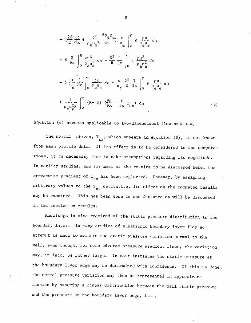
Equation (8) becomes applicable to two-dimensional flow as R .

The normal stress, Txx, which appears in equation (8), is not known

from mean profile data. If its effect is to be considered in the computa-

tions, it is necessary then to make assumptions regarding its magnitude.

In earlier studies, and for most of the results to be discussed here, the

streamwise gradient of Txx has been neglected. However, by assigning

arbitrary values to the Txx derivative, its effect on the computed results

may be examined. This has been done in one instance as will be discussed

in the section on results.

Knowledge is also required of the static pressure distribution in the

boundary layer. In many studies of supersonic boundary layer flow no

attempt is made to measure the static pressure variation normal to the

wall, even though, for some adverse pressure gradient flows, the variation

may, in fact, be rather large. In most instances the static pressure at

the boundary layer edge may be determined with confidence. If this is done,

the normal pressure variation may then be represented in approximate

fashion by assuming a linear distribution between the wall static pressure

and the pressure at the boundary layer edge, i.e.,

9

P = P + n (pe - Pw) (9)

Examination of equation (8) shows that an accurate value of boundary

layer growth rate is very important for the calculation of the shear

stress. However, precise determination of the boundary layer thickness

from experimental mean data is difficult. It is even more difficult to

evaluate the boundary layer growth rate accurately. This problem may be

avoided by using the condition that the shear stress diminishes to zero

at the boundary layer edge and solving equation (8) for d6/dx:

d6 f 6 dp 2 + ddS Cf (. dPeUe 6 dR l pu2dx 2 p 2 dx R dx u2

ee ee

2 dpu 2 1 u26 ee _ PU p[n+d

P u2R dx p uee J ee

6 dR 6 dpe e 1 dP ee pu_du + +62 p+ u dp u dx Pu puR dx puee o ee ee o ee

x p u2 R xx fp u2 x d.P ee o ee o ee

+62 r pu 6 w 6R x pu p u2 dx 2Ro ee ee

d(P -P 1

+ ( - (10)/ 1 d)

2 dx 2 3R R2pu o PU

p u2

e e

1 2 t1 1pu pu R pu

0 ee o ee o ee

+ 2 ~ 2 3R (10)puee

10

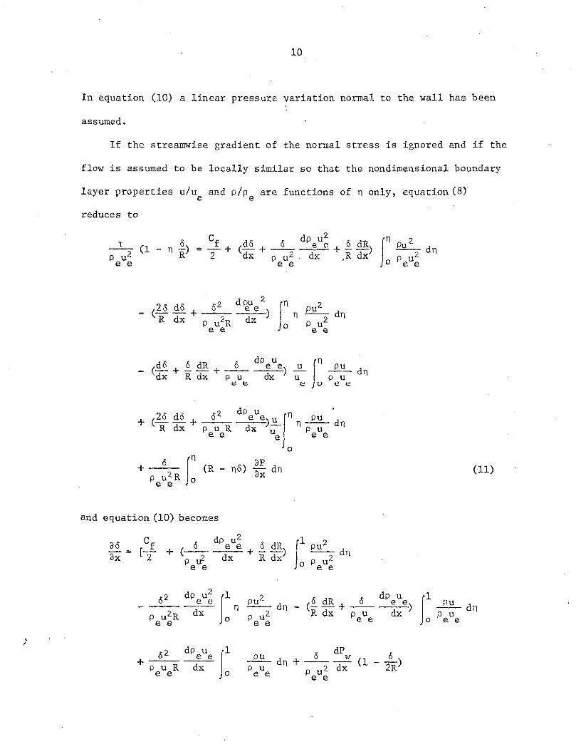
In equation (10) a linear pressure variation normal to the wall has been

assumed.

If the streamwise gradient of the normal stress is ignored and if the

flow is assumed to be locally similar so that the nondimensional boundary

layer properties u/ue and p/pe are functions of n only, equation (8)

reduces to

_ 6 Cf d6 6 dPeue 6 dR r pu2

(1 - ) = -+ ( + 2 d + R ) dp 2 2 ) d. p u2. dx R dx p uee ee J0 ee

26 dS 62 dpue2 p2- 6 + e ) dnR d p2R dx p u2

ee ee

d 6 dR 6 dp e u PuSdx R dx pu dx u pu

26 d6 62 dPeue u pud) puR dx p uee ee

0

+ j n(R - nS) -dn (11)p u2 R o @xee

and equation (10) becomes

C dp u2 1 2_6 Cf 6 e e 6 dR pu d- = [- + - + ) d uax 2 p u dx R dx

ee ee

2 dpu 2 1 2 dR dp u 1

epe e e e eee ee

2 dPe e pu 6 w 6+ d e (1 )

p u R dx Pu u 2 dx 2Ree o ee ee

Sed(P-P) e2-- e w 1- I pu dri

S2 dx 2 3R R P u2

SPu 2 d + p d n dn] (12)2 pu R pu

S e ee

Equation (11) is identical to the expression used by Bushnell and Morris1

in their computations of turbulent shear stress.

Before solving for the shear stress from either equation (8) or (11)

it is also necessary to know the coefficient of skin friction. This may

be obtained by using the wall-wake velocity profile proposed by Sun and

Childs . The wall-wake velocity profile for isoenergetic flow may be

written as

a 1/2

= sin {arc sin a (1 + (n n +

e a e

- 2 In (1 + (-a)1 / 2) H U (1 + cos nl)],} (13)a K u*

e

where

u* 6uS u 1 6ue 0.614

T [2 1 In (-) - 5.1+ ] (14)K 2 u K aK

T W

and

u Cf a 1/2 1/2

= ( -) arc sin a (15)u* 2 1-o

e

As has been reported in Reference 7, the use of a = 1 in equations (13) and

(14) results in a profile which provides a good representation of the

boundary layer velocity distribution. The method of least-squares may be

12

used to fit the wall-wake profile to the experimental mean velocity pro-

files to provides values of Cf and to provide a smoothed representation

of the mean velocity distribution.

The eddy viscosity and mixing length distributions are also of great

interest in the study of turbulent boundary layer flow. In terms of the

shear stress as computed from mean flow data, the eddy viscosity may be

written as

S 1 (T- uy) (16)u 6 u 6 p u/y (16)e e

and the mixing length as

R 1 T-P u/ y]1/27 = (17)6 p(u/ay)2

In the region close to the wall the mixing length may be approximated by

9 = ky (18)

where k is a constant.

In terms of turbulence measurements the eddy viscosity may be expressed as

C 1 -<u'v'>U = I u/ y• (19)u 6 u 6 au/3ye e

and the mixing length as

2 1 -<u'v'> 1/2l I . (20)6= 6 (u/y) 2

A comparison of eddy viscosity and mixing length values as determined from

turbulence measurements and from mean flow shear stress computations is

given in the section on results.

13

III. RESULTS

A computer program has been developed to carry out the required

numerical calculations. In carrying out the computations for the flow

downstream of the shock wave-boundary layer interactions, the departure

from local similarity has been taken into account. For purposes of

comparison, however, computations based on local similarity have also been

made. The effect of static pressure variation normal to the wall has also

been considered for the downstream stations by assuming a linear variation

in pressure. In these computations the static pressure at the boundary

layer edge has been computed from the free stream total pressure and pitot

pressure, with appropriate allowance made for the loss in total pressure

across the shock system. As was mentioned in the previous section, the

mean velocity profiles may be smoothed by using a least squares fit of the

wall-wake velocity profile to the experimental profiles. Computations have

been made for both smoothed and unsmoothed profiles. The integration

process for the smoothed data should be more accurate because it is possible

to use smaller step sizes. On the other hand, the shear stress computed

from the smoothed profiles is valid only if the wall-wake profile provides

a good representation of the actual velocity distribution.

In obtaining the density and velocity profiles from the pitot pressure

profiles for the investigation by Rose and Johnson4 '5 , the total tempera-

ture was assumed to be constant across the boundary layer. In the axisym-

metric study by Rose 6 total temperature measurements were available. For

this case calculations of the shear stress distributions were made for both

the measured total temperature distribution and for a constant total tem-

perature. The results differed from each other only slightly.

14

Figure 1 shows shear stress distributions computed for an upstream,

(x = 5.375 cm) station in Johnson's and Rose's investigation, along with

their shear stress data from the hot-wire anemometer and the laser

velocimeter measurements. The computed shear values which are shown

have been obtained from equation (11) and auxiliary equation (12), i.e.,

under the assumption of local similarity. As is shown the calculated

results agree quite well over much of the boundary layer, with the meas-

ured results obtained with the laser velocimeter. The differences between

the calculated results and the hot-wire results are greater. For both

the hot-wire and laser velocimeter measurements the peak values of shear

stress are seen to occur substantially farther from the wall than is

observed for the calculated distributions. Also shown in the figure are

values of the wall shear stress as determined by a least squares fit of

the wall-wake profile to the mean data and as measured by a Preston tube.

The agreement between the two shear stress values is good.

The wall-wake profile as given by equation (13) can be reduced to

a profile proposed earlier by Maise.' and McDonald8 if H is taken to be

equal to 5.0 and if a + m. For purposes of comparison, the Maise-

McDonald profile has been used to compute shear stress values. As is

shown, this results in shear values which are substantially lower than

those obtained with a = 1 in equation (13) or with the unsmoothed data.

Computations have also been carried out for the data of Rose and

Johnson for a station downstream of the shock wave-boundary layer inter-

action (x = 9.375 cm). Several sets of computations have been made from

the mean data. In one set local similarity has been assumed. Equations

(11) and (12) have then been used to carry out computations for both

15

wall-wake smoothed profile and a profile as measured. In other computations

local similarity of profiles has not been assumed. For these cases re-

sults have been obtained for both smoothed and unsmoothed profiles and both

linear and constant static pressure distribution across the boundary layer.

The results are shown in Figures 2 and 3. Figure 2 shows that the meas-

ured shear stress values obtained by the two experimental techniques are

in quite good agreement. These in turn agree reasonably well with

the computed values obtained by using smoothed nonsimilar profiles and the

assumption of a linear pressure variation across the boundary layer. There

is considerable difference between the results for the smoothed and un-

smoothed profiles with the peak shear stress value for the unsmoothed pro-

file occurring lower in the boundary layer. As was stated earlier, the

numerical integration process should be more accurate for the smoothed

profiles. On the other hand, the results obtained from the wall-wake

profiles are valid only if the profiles provide accurate representations

of the actual velocity distributions. A comparison of the computed

velocity distributions with the corresponding wall-wake profiles is shown

in Figure 4. The differences between the two are small, pointing to the

sensitivity of the computed shear stress values to small velocity differ-

ences.

As is shown in Figure 3, the results obtained under the assumption

of local similarity are markedly different from those determined when

similarity is not assumed. The peak shear stress levels computed assuming

local similarity are less than half the values computed when similarity

is not assumed. Furthermore, the shapes of the shear stress distribution

curves are quite different. These results occur even though the differences

16

between profiles at two closely spaced stations are small. Figure 5

shows comparisons of density and velocity profiles from Rose's and

Johnson's study for streamwise stations located approximately one boundary

layer thickness apart. Although the profiles appear at first glance to be

quite similar, striking differences are found for the computed shear

stress distributions.

In the investigation by Rose 6 of an adiabatic axisymmetric shock

wave-boundary layer interaction the free stream flow was nominally at M = 4

and the shock wave was generated by a 9-degree half-angle cone placed at

zero angle of attack on the centerline of the 5.28 cm diameter tunnel. The

shock strength was just below that required to produce boundary layer

separation. For this flow a substantial adverse pressure gradient existed

downstream of the interaction. As was stated earlier, the turbulence data

were obtained with a hot-wire anemometer.

Figure 6 shows results for a station upstream of the interaction

where there was no pressure gradient. The shear stress distribution has

been computed from mean velocity and density profiles under the assumption

of local similarity and constant static pressure across the boundary layer.

As is shown, reasonably good agreement between computed and measured shear

stress values is obtained, although the differences observed for the Rose-

Johnson4,5 data are found to exist here as well. That is, the hot-wire

anemometer results show higher levels than the computed values in the outer

part of the boundary layer, and the peak value of the computed shear stress

is much closer to the wall than was found to be the case from the direct

measurements.

17

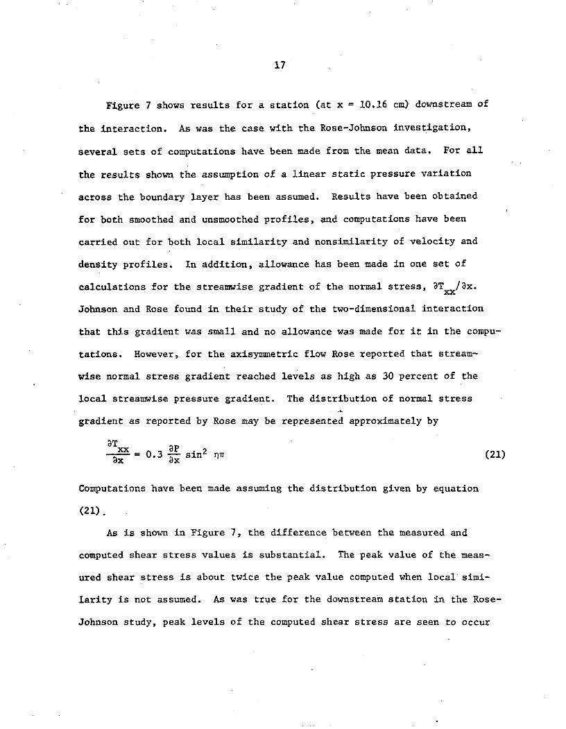
Figure 7 shows results for a station (at x = 10.16 cm) downstream of

the interaction. As was the case with the Rose-Johnson investigation,

several sets of computations have been made from the mean data. For all

the results shown the assumption of a linear static pressure variation

across the boundary layer has been assumed. Results have been obtained

for both smoothed and unsmoothed profiles, and computations have been

carried out for both local similarity and nonsimilarity of velocity and

density profiles. In addition, allowance has been made in one set of

calculations for the streamwise gradient of the normal stress, T xx/ax.

Johnson and Rose found in their study of the two-dimensional interaction

that this gradient was small and no allowance was made for it in the compu-

tations. However, for the axisymmetric flow Rose reported that stream-

wise normal stress gradient reached levels as high as 30 percent of the

local streamwise pressure gradient. The distribution of normal stress

gradient as reported by Rose may be represented approximately by

aT0.3 - sin2 n (21)8xax

Computations have been made assuming the distribution given by equation

(21).

As is shown in Figure 7, the difference between the measured and

computed shear stress values is substantial. The peak value of the meas-

ured shear stress is about twice the peak value computed when local simi-

larity is not assumed. As was true for the downstream station in the Rose-

Johnson study, peak levels of the computed shear stress are seen to occur

18

considerably closer to the wall than is observed in the measurements. It

has not yet been possible to determine the causes for the rather large

differences between the peak levels of the computed and measured shear

stress distributions. Additional hot-wire studies are underway for the

axisymmetric flow, as are attempts to improve upon the computational

techniques.

As was the case for the downstream station in the Rose-Johnson4' 5

investigation, the assumption of local similarity leads to shear stress

levels which are on the order of only one-half those determined when

similarity is not assumed. As is shown in Figure 7, consideration of the

streamwise normal stress gradient in the computations results in shear

stress levels which differ only very slightly from those obtained when

the gradient is ignored.

It should be pointed out that Rose , in obtaining his downstream

data, moved the cone along the axis of the tunnel and obtained the pitot

measurements at a fixed axial station. The question arises, then, of

how the computed shear stress distributions would compare with those

obtained if the cone had been kept at one station and the pitot tube had

been traversed axially. As a check on this, data were examined from a

study by Seebaugh in which the cone was held fixed and the probe was

translated. Seebaugh's study was conducted in a 5.16 cm diameter round

tunnel with a free-stream Mach number of 3.78. He used a 10-degree half-

angle cone. The results are shown in Figure 8. As is apparent, the shear

stress distributions are quite comparable to those obtained from Rose's

mean flow data.

19

The distributions of eddy viscosity and mixing length for the invest

tigations under consideration are shown in Figures 9-12. The results,

of course, reflect the differences between the measured and computed

values of shear stress as discussed earlier. Computed results are shown

for both smoothed and unsmoothed profiles. For the stations upstream of

the shock wave-boundary layer interactions the shear stress distributions

used in obtaining the values of eddy viscosity and mixing length have

been determined under the assumption of local similarity. For the down-

stream stations, the lack of local similarity in the velocity and

density profiles has been taken into account and a linear static pressure

variation across the boundary layer has been assumed.

The eddy viscosity distributions for the Rose-Johnson investigation

are shown in Figure 9. Near the wall moderately good agreement is

observed between eddy viscosities based on computed shear stress value

and those based on measurements. From y/6 .= 0.2 outward, however, the

differences become substantial. The values based on experimental shear

stress show considerable scatter as do those based on the point-by-point

mean data. In contrast the results based o;i the wall-wake smoothed

velocity profile are smooth, as would be expected.

The mixing length distributions for the Rose-Johnson4, 5 investigation

are shown in Figure 10. Near the wall the values of mixing length are

described reasonably well by the relationship Z = 0.4y. From y/6 = 0.2

outward a certain amount of scatter in the results is apparent. For the

upstream station (x = 5.375 cm), however, the computed distribution based

on the wall-wake profile agrees with the results based on turbulence meas-

urements reasonably well. For the downstream station (x = 9.375 cm) the

20

values of Z/6 based on the wall-wake profile are consistently higher than

those based on the turbulence measurements or on the unsmoothed mean data.

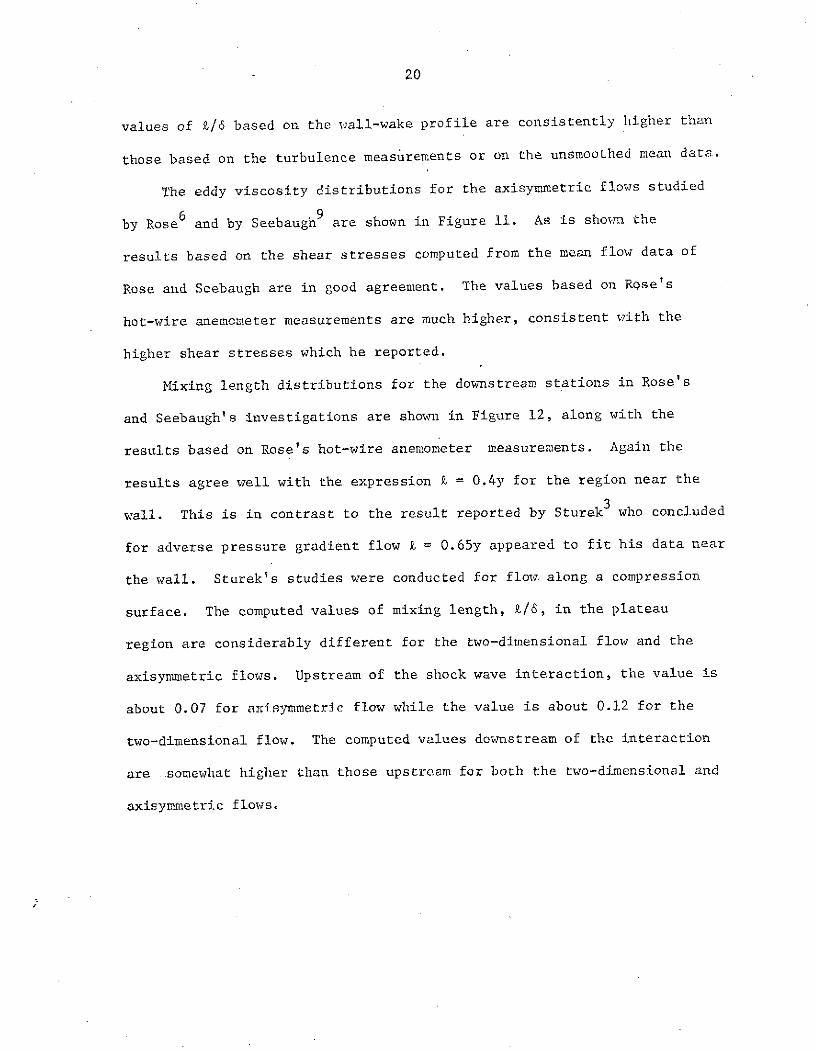
The eddy viscosity distributions for the axisymmetric flows studied

by Rose 6 and by Seebaugh9 are shown in Figure 11. As is shown the

results based on the shear stresses computed from the mean flow data of

Rose and Seebaugh are in good agreement. The values based on Rose's

hot-wire anemometer measurements are much higher, consistent with the

higher shear stresses which he reported.

Mixing length distributions for the downstream stations in Rose's

and Seebaugh's investigations are shown in Figure 12, along with the

results based on Rose's hot-wire anemometer measurements. Again the

results agree well with the expression k = 0.4y for the region near the

wall. This is in contrast to the result reported by Sturek3 who concluded

for adverse pressure gradient flow £ = 0.65y appeared to fit his data near

the wall. Sturek's studies were conducted for flow along a compression

surface. The computed values of mixing length, Z/6, in the plateau

region are considerably different for the two-dimensional flow and the

axisymmetric flows. Upstream of the shock wave interaction, the value is

about 0.07 for axisymmetric flow while the value is about 0.12 for the

two-dimensional flow. The computed values downstream of the interaction

are somewhat higher than those upstream for both the two-dimensional and

axisymmetric flows.

21

IV. CONCLUSIONS

A method of computing shear stress distribution from experimental

mean profile data in compressible turbulent boundary layer flow has been

developed. The method is different from those previously reported in

that integrated mass and momentum flux profiles and differentials of

these integral quantities are used in the computations so that local

evaluation of the streamwise velocity gradient is not necessary. The

method has been found to yield results which are in reasonably good agree-

ment with directly measured turbulence data for two-dimensional adiabatic

boundary layer flow in the regions upstream and downstream of an oblique

shock wave interaction. The computed results are very sensitive to the

accuracy of the numerical integrations required in the computational

procedure and to the mean property distributions in the boundary layer.

The assumption of local similarity may canse lrge Prrors in computed

shear stress values for flows subjected to pressure gradients, even though

adjacent profiles of the mean properties appear to be quite similar.

The shear stress levels are quite sensitive to the static pressure dis-

tribution normal to the wall. The effect of the streamwise gradient of the

normal stress on the computed results is small and apparently may be

neglected. The value of the constant k in the expression k = ky for

the mixing length in the region near the wall remains close to 0.4 for

adverse pressure gradient flows along a flat surface. In view of the

rather substantial differences between results based on mean flow measure-

ments and those based on turbulence measurements in an axisymmetric

adverse pressure gradient flow, further study of this flow is needed.

22

REFERENCES

1. Bushnell, D.M. and Morris, D.J., "Shear-Stress, Eddy-Viscosity andMixing Length Distributions in Hypersonic Turbulent BoundaryLayers," NASA TX-2310, 1971.

2. Horstman, C.C. and Owen, F.K., "Turbulent Properties of a CompressibleBoundary Layer," AIAA Journal, vol. 10, no. 11, November 1972, pp.1418-1424.

3. Sturek, W.B., "Calculations of Turbulent Shear Stress in SupersonicTurbulent Boundary Layer Zero and Adverse Pressure Gradient Flow,"AIAA Paper No. 73-166, January 1973.

4. Johnson, D.A. and Rose, W.C., "Measurement of Turbulent TransportProperties in a Supersonic Boundary-Layer Flow Using LaserVelocimeter and Hot Wire Anemometer Techniques," AIAA Paper 73-1045,Seattle, Washington, 1973.

5. Rose, W.C. and Johnson, D.A., "A Study of Shock Wave TurbulentBoundary Layer Interaction Using Laser Velocimeter and Hot WireAnemometer Techniques," AIAA Paper 74-95, Washington, D.C., 1974.

6. Rose, W.C., "The Behavior of a Compressible Turbulent Boundary Layerin a Shock-Wave-Induced Adverse Pressure Gradient," TND-7092, NASA,March 1973.

7. Sun, C.C. and Childs, M.E., "A Modified Wall-Wake Velocity Profile forTurbulent Compressible Boundary Layers," Journal of Aircraft, vol.10, no. 6, June 1973, pp. 381-383.

8. Maise, G. and McDonald, H., "Mixing Length and Kinematic EddyViscosity in a Compressible Boundary Layer," AIAA Journal, vol. 6,no. 1, January 1968, pp. 73-80.

9. Seebaugh, W.R., "An Investigation of the Interaction of a Shock Waveand a Turbulent Boundary Layer in Axially Symmeltric Internal FlowIncluding the Effect of Mass Bleed," PhD Thesis, 1968, University ofWashington, Seattle, Washington.

23

Figure 1. Turbulent shear stress distribution upstreamof a shock wave-boundary layer interaction,two-dimensional tunnel [4]

Figure 2. Turbulent shear stress distributiondownstream of a shock wave-boundarylayer interaction, two-dimensionaltunnel [5]

Figure 3. Effect of static pressure distribution andself-similarity on shear stress distributionin a turbulent boundary layer downstream ofa shock wave interaction [5]

Figure 4. Velocity profiles and wall-wake representationsdownstream of a shock wave-boundary layerinteraction [5]

Figure 5. Density and velocity profiles downstream of ashock 7ave-boundary layer interaction [5]

Figure 6. Turbulent shear stress distribution upstreamof a shock wave-boundary layer interaction,axisymmetric tunnel [6]

Figure 7. Turbulent shear stress distribution downstreamof a shock wave boundary layer interaction,axisymmetric tunnel [6]

Figure 8. Turbulent shear stress distribution downstreamof a shock wave-boundary layer interaction,axisymmetric tunnel [9]

Figure 9. Eddy viscosity distribution for the two-dimensionalflow of Rose and Johnson [4,5]

24

Figure 10. Mixing length distribution for the two-dimensionalflow of Rose and Johnson [4,5]

Figure 11. Eddy viscosity distributions for theaxisynummetric flows of Rose [6] andSeebaugh [9]

Figure 12. Mixing length distributions for theaxisymmetric flows of Rose [6] andSeebaugh [9]

2.5

2.0 Measured - [- p<u'v'>/P u2 ] x 103

O laser velocimeter [4]

1- hot-wire anemometer [4]

1. O A Computed - [(r - pau/9y)/P u2 ] x 103

0 mean data, eq. (11)0 A

-- wall-wake presentation of mean

. \ data, eq. (11)

---- Maise-McDonald profile repre-sentation of mean data [8]

0 A

S O0-Tw computed from wall-wake profile

0.5" w measured with Preston Tube

'ao 1

i " I

0.0 0.5 1.0

- p<u'v'>/p Ue ] x 10 3 , [(. - jau/ay)/p u2] x 10 3

ee e

Measured - [- p<u'v'>/p u ] x 103

ee

O laser velocimeter [5]

2.5 A hot-wire anemometer [5]

Computed - [(T - Pau/y)/Pe u ] x 103

O. mean data, linear static pressure distribution,

Eq. (8)

2.0-- wall-wake representation of mean data, linear

static pressure distribution, Eq. (8)

- t computed from wall-wake profile

1.5 0

1.0 -

0.5 A 0

0

1

0.0 0.5 1.0

[- p<u'v'>/p u2] x 103, [(T - pau/ay)/Pe u2 ] x 103ee ee

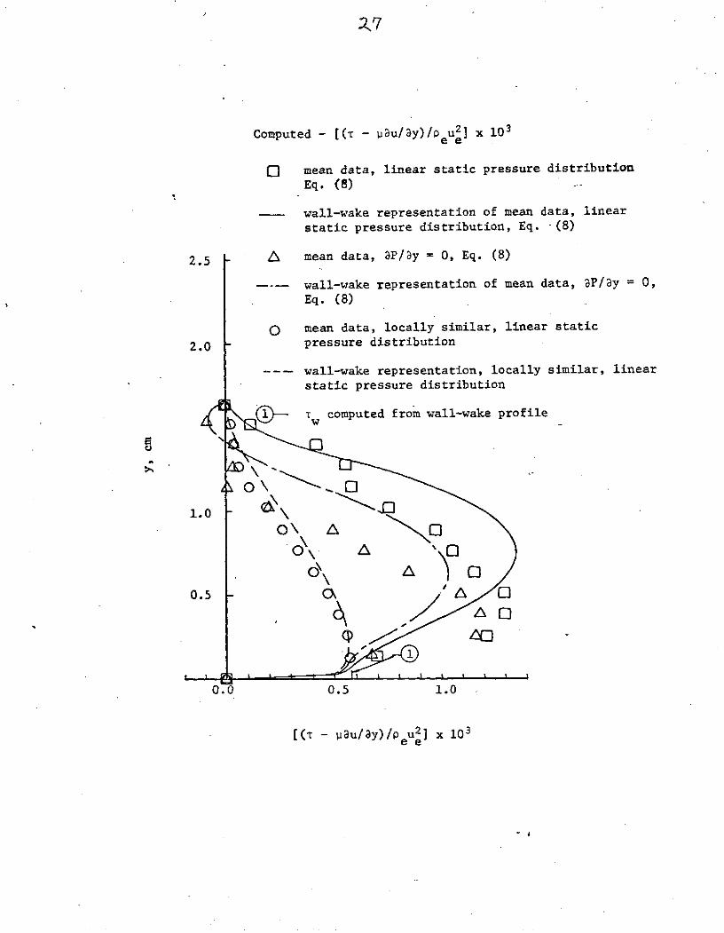
Computed - [(T - u3u/3y)/eu2] x 103

o mean data, linear static pressure distributionEq. (8)

wall-wake representation of mean data, linearstatic pressure distribution, Eq. -(8)

2.5 A mean data, 3P/y = 0, Eq. (8)

wall-wake representation of mean data, 3P/ay = 0,Eq. (8)

O mean data, locally similar, linear static

2.0 pressure distribution

---- wall-wake representation, locally similar, linearstatic pressure distribution

-- tw computed from wall-wake profile

1.0

0\ \o

0.5 - CX ' Z ~

10

0.0 0.5 1.0

[(t - pau/ay)/p u 2 ] x 10 3ee

1.0 x = 8.105 cm

0 measured data

wall-wake representation

x = 9.375 cm

A measured data

wall-wake representation

0.5

0.0

0.0 0.5 1.0

u/ue

1.0 x = 8.105 cm

O velocity

A density

x = 9.375 cm

/ velocity,

C3 density

0.5'

0.00.0 0.5- 1.0

u/ue , P/pe

Measured - [- p<u'v'>/p U 2 ] x 103

A hot-wire anemometer [6]

Computed - [(T - 1Vu/ay)/eUZe ] x 103

0.4 0 mean data, Eq. (11)

- wall-wake representation of mean data, Eq. (11)

0.3 A t computed from wall-wake profile

0.2

0.1 A

0.00.0 1.0 2.0 3.0 4.0

[- p<u'v'>/PeU2]x 10 3 , [(t - ~a fp u 2]x 103e ee

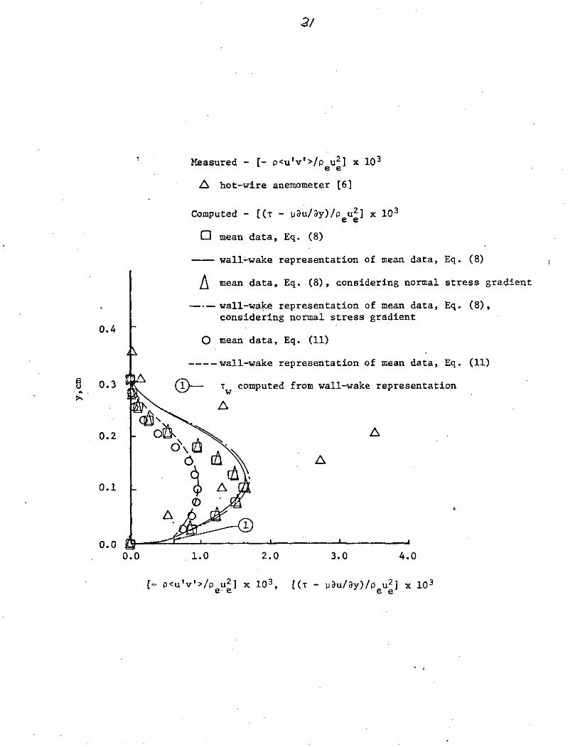
Measured - [- p<u'v'>/p u2] x 103ee

a hot-wire anemometer [6]

Computed - [(T - pau/ay)/Peu2 ] x 103

o mean data, Eq. (8)

-- wall-wake representation of mean data, Eq. (8)

A mean data, Eq. (8), considering normal stress gradient

--- wall-wake representation of mean data, Eq. (8),considering normal stress gradient

0.4O mean data, Eq. (11)

---- wall-wake representation of mean data, Eq. (11)

0.3 T- w computed from wall-wake representation

0.2 - O

0.1 - ( a

1

0.00.0 1.0 2.0 3.0 4.0

[- p<u'v'>/p u2] x 103 , [(T - paulay)/ u2 ] x 103eue ee

Computed - [(T - Pau/y)/p u2 ] x 10 3

ee

O mean data, Eq. (8)

- wall-wake representation of mean data, Eq. (8)0.4

O mean data, Eq. (11)

--- wall-wake representation of mean data, Eq. (11)

0.3 - - Tw computed from wall-wake representation

0.2

0.1

0. 00.0 1.0 2.0 3.0 4.0

[(r - Pau/3y)/P u2 ) x 10 3

e- e

Eddy Viscosity based on measured shear stress

0 x = 5.375 cm, laser velocimeter [4]

O x = 9.375 cm, laser velocimeter [5]

A x = 5.375 cm, hot-wire anemometer

A x = 9.375 cm, hot-wire anemometer

Eddy Viscosity based on computed shear stress

* x = 5.375 cm, computed from mean data, Eq. (8)

[] x = 9.375 cm, computed from mean data, Eq. (8)

x = 5.379 cm, computed from wall-wake representation ofmean data, Eq. (8)

x = 9.375 cm, computed from wall-wake representation8.0 of mean data, Eq. (8)

0

Oo

6.0/

r-I - A

N2.0 a

0.00.0 0.5 1.0

y/6

Mixing Length based on measured shear stress

0 x = 5.375 cm, laser velocimeter [4]

O x = 9.375 cm, laser velocimeter [5]

A x = 5.375 cm, hot-wire anemometer

A x = 9.375 cm, hot-wire anemometer

Mixing Length based on computed shear stress

S x = 5.375 cm, computed from mean data, Eq. (8)

[] x = 9.375 cm, computed from mean data, Eq. (8)

-- x = 5.375 cm, computed from wall-wake representation0.2 of mean data, Eq. (8)

x = 9.375 cm, computed from wall-wake representationof mean data, Eq. (8)

I = 0.4y

0.1 0 O

0.00.0 0.5 1.0

y/6

Eddy Viscosity based on measured shear stress

A x = 6.60 cm, hot-wire anemometer [6]

A x = 10.16 cm, hot-wire anemometer [6]

Eddy Viscosity based on computed shear stress

* x = 6.60 cm, computed from mean data [6]

- x = 6.60 cm, computed from wall-wake representationof mean data

O x = 10.16 cm, computed from mean data [6]

x = 10.16 cm, computed from wall-wake representationof mean data [6]

o x = 9.62 cm, computed from mean data [9]

8.0 ---- x = 9.62 cm, computed from wall-wake representationof mean data [9]

6.0

4.0

0.0 0.5 1.0

y/6y/S

Mixing Length based on measured shear stress

A x = 6.60 cm, hot-wire anemometer [6]

a x = 10.60 cm, hot-wire anemometer [6]

Mixing Length based on computed shear stress

* x = 6.60 cm, computed from mean data [6]

- x = 6.60 cm, computed from wall-wake representationof mean data [6]

o x = 10.16 cm, computed from mean data [6]

--- x = 10.16 cm, computed from wall-wake representationof mean data [6]

O x = 9.62 cm, computed from mean data [9]

-----x = 9.62 cm, computed from wall-wake representation0.2 of mean data [9]

A A

I = 0.4y 0

'0

0.1

0.0

0.0 0.5 1.0

y/6