1

Calculation of Ground State Potential Energy Surface and Observables for a Diatomic

Molecule

1. Introduction

2. Electronic structure methods

3. Kinds of calculations

4. Experimental

5. Lab report

6. Appendices

Electronic structure software, sometimes called computational chemistry software, is used in many areas of chemistry

and biochemistry. This software calculates the electronic wavefunction or probability density for a molecule. Based

on this, many useful properties (e.g. total energy, equilibrium bond length, vibrational frequency) may be reported in

the output.

In this lab, you will calculate the potential energy surface (PES) for a diatomic molecule. From the PES, you will

determine the equilibrium bond length (re), force constant (k), vibrational frequency (), and bond dissociation energy

(De and Do) of the molecule.

Introduction

The idea of a PES rests on the fact that electrons, being much less massive that atomic nuclei, adjust their positions

almost instantaneously to any change in the nuclear coordinates. A PES is calculated by treating this adjustment as if

it were fully instantaneous, an assumption called the Born-Oppenheimer (BO) approximation. You will calculate the

PES for a diatomic molecule for the electronic ground state (molecules have many different electronic states; each

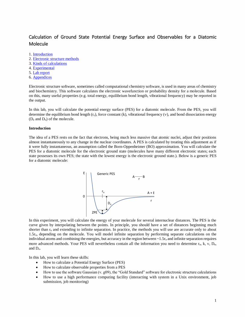
state possesses its own PES; the state with the lowest energy is the electronic ground state.). Below is a generic PES

for a diatomic molecule:

In this experiment, you will calculate the energy of your molecule for several internuclear distances. The PES is the

curve given by interpolating between the points. In principle, you should have a set of distances beginning much

shorter than re and extending to infinite separation. In practice, the methods you will use are accurate only to about

1.5ro, depending on the molecule. You will model infinite separation by performing separate calculations on the

individual atoms and combining the energies, but accuracy in the region between ~1.5re and infinite separation requires

more advanced methods. Your PES will nevertheless contain all the information you need to determine re, k, , De,

and Do.

In this lab, you will learn these skills:

How to calculate a Potential Energy Surface (PES)

How to calculate observable properties from a PES

How to use the software Gaussian (v. g09), the “Gold Standard” software for electronic structure calculations

How to use a high performance computing facility (interacting with system in a Unix environment, job

submission, job monitoring)

Do

ZPE

E

r

ro

Generic PESA B

r

A + B0

2

Electronic Structure Methods

There are many electronic structure methods available. All invoke some form of approximation for all molecules or

atoms other than the H atom. You will be using a method designated B3LYP/6-31G* unless your molecule contains

an H atom, in which case you will use B3LYP/6-31G**. The part preceding the forward slash specifies the method

proper; the part after the forward slash is the basis set. The method proper and basis set will be discussed in somewhat

greater depth at the beginning of the lab.

Kinds of calculations

You will perform four kinds of calculations to determine your PES and the associated observables. It is important to

do the calculations in the order given, as they will most sense when learned that way.

Single point energy (sp): Calculates the energy for one specified value of the internuclear distance (or more

generally for larger molecules, of the geometry).

PES scan (scan): Calculates the energy for a set of internuclear distances. Typically, one specifies the initial

distance, the number of steps, and the amount by which the distance is incremented from step to step. (For

larger molecules, one may also scan along values of other coordinates, such as bond angles.)

Geometry optimization (opt): Determines the internuclear distance for which the energy is at a minimum; in

other words, determines re. (When the molecule contains more than two atoms, all the atomic positions are

systematically adjusted until the conformation (geometry) has the lowest energy possible. It should be noted

that energy barriers cannot be crossed in geometry optimization. Therefore, the outputted conformation may

represent a local but not a global energy minimum. This is not an issue for a diatomic molecule.)

Frequency (freq): Calculates the vibrational frequency for the given internuclear distance. The inputted

geometry must represent an energy minimum; otherwise, the frequency calculated may not be meaningful.

However, this will not be an issue for you because you will issue a command (opt freq) that first does a

geometry optimization to locate the energy minimum, and then calculates the vibrational frequency. (Note

that when computations are done on larger molecules, there will be several different vibrational modes, each

having its own vibrational frequency.)

Experimental

1. SINGLE POINT ENERGIES (SP): Perform single point calculations for your diatomic molecule using the

distances 0.5, 1.0, 1.5, and 2.0 Å. Doing so is mainly for practice with single point calculations, but it also

serves as verification of the results of the PES scan (below). If there is a difference between a single point

energy and the PES scan, it indicates either that an error was made or that the calculated energy cannot be

trusted at that distance. Also perform single point calculations on the individual atoms from which your

molecule is made (one at a time, for each atom). It will be critical to determine the multiplicity (M) for your

molecule. This will be discussed at the beginning of the lab.

2. PES SCAN (SCAN): Perform a scan from a distance of 0.5 Å out to a distance of 2.0 Å, in increments of 0.1

Å. The outer distance may need to adjusted, depending on your molecule. Check whether the energies from

the scan are consistent with the single-point energies from step (1). Once you reach distances beyond the

attractive well, you may find that the energies of individual points are larger than the combined energy of the

individual atoms. That is probably just an indication that the method gives inaccurate results beyond the

attractive well. You should, though, be able to get several points on either side of the energy minimum, as

well as points in the vicinity of the repulsive wall.

3. GEOMETRY OPTIMIZATION + FREQUENCY (OPT FREQ): Perform a combined geometry optimization

/ vibrational frequency calculation by inputting a distance near the energy minimum identified in step (2) and

placing the “opt freq” command in the Gaussian script. The exact value of the internuclear distance that you

start with is not important, because the software will locate the minimum-energy geometry.

Lab report

1. Make a table in Excel (or similar program) of energy vs distance for step (2) of the Experimental. The last

row in your table should be the combined energies of the individual atoms from Experimental step (1); it is

not practical to assign them a distance of infinity when making a graph, so use the number 5 (or a similar

number) instead. Create a column in which all energies are given in electron volts (eV), and all energies are

relative to the energy of the infinitely separated atoms (subtract the energy of infinitely separated atoms from

3

all the energies; the energy of infinitely separated atoms will then appear as zero). Also make a table of the

single point energies for the diatomic molecule in Experimental step (1), and verify that they are in agreement

with the PES scan. If there is disagreement, be sure your calculations were done correctly, and disagreement

remains, note the distance(s) at which it occurs.

2. Make a plot of energy vs distance from the first table in Lab Report step (1), using the eV values with infinite

separation (which will actually show up as ~5 Å) representing the zero of energy. This is your PES.

3. Make a quadratic fit to the 5 points with lowest energy from your plot. Display the fitted curve and the

equation of the fit (including the R2 value). You may want to create a separate graph to do this. (DO NOT

TRY TO FIT A QUADRATIC EQUATION TO ALL OF YOUR DATA POINTS. The fit will be very poor,

and you will not be able to extract a meaningful data from it.)

4. The force constant, k, is the second derivative of the fitted quadratic function, and re is the distance that

corresponds to the minimum energy. Determine k and re. (Why is the force constant equal to the second

derivative of the fitted quadratic function? Think of the formula for a harmonic potential energy function,

and take the second derivative.)

5. Also determine the vibrational frequency () and the zero-point energy (ZPE). You may need to consult notes

from the lecture class or your text for the needed equations.

6. Finally, determine the bond dissociation energy from the minimum in the potential energy curve, De. Also

find Do. Do is the difference between the energy of the individual atoms and the energy of the molecule at

the equilibrium bond distance, including the zero-point energy:

De = (EA + EB) – EAB,re Do = De - ZPE

where 𝐸𝐴 is the energy of atom A, 𝐸𝐵 is the energy of atom B, and 𝐸𝐴𝐵,𝑟𝑒 is the energy of the diatomic

molecule at the equilibrium bond distance.

7. The “opt freq” calculation will also give you values for re, , and the ZPE. These will probably be more

accurate than those determined directly from your calculated PES because the geometry optimization part of

the command (opt) effectively uses a finer grid than 0.1 Å near the energy minimum to locate the minimum

precisely. Determine the percent difference between your values from step (4) and those obtained with “opt

freq.” Comment on the magnitude of the differences and their origin.

8. In the literature, look up experimental values for re, , and De. One good source for re and is the NIST

Webbook. For Do, you may need to search for the “bond dissociation energy” of your molecule. Enter your

molecule in the formula section and check “constants of diatomic molecules.” You will be given constants

for excited states as well as the ground state. The ground state will be the last one listed, and its symbol begins

with “X”. Your instructor will explain to you how to locate the multiplicity (M) in the symbol. Compare the

values for re, , De, and Do that you calculated in step (7) (the ones from the “opt freq” calculation) with the

experimental values. Again, make the comparison in terms of percent error. Discuss which observable(s)

is/are calculated most accurately.

9. You may wonder about the purpose of performing calculations. After all, the experimental data for the

observables in your case is probably of higher quality than the experimental data. Can you think of any value

added by calculations? Discuss this. You may want to talk with your instructor.

4

Appendices

1. Access to FIU’s HPC Cluster via hpcgui.fiu

2. Gaussian input files (scripts)

3. Submission file for Gaussian scripts

4. Gaussian output file: finding the results you want

5. Alternative ways to access FIU’s HPC cluster

Appendix 1: Access to FIU’s HPC cluster via hpcgui.fiu

The easiest access to FIU’s High Performance Computing (HPC) facility is via the web-based remote

terminal. Go to hpcgui.fiu.edu in your browser and login with you FIU account credentials. From home (or outside

FIU) campus, the site is accessible if you use FIU’s VPN.

On the Clusters tab choose >_Panther Shell Access to access an HPC terminal window, which will allow you to

submit GAUSSIAN calculation jobs to HPC:

5

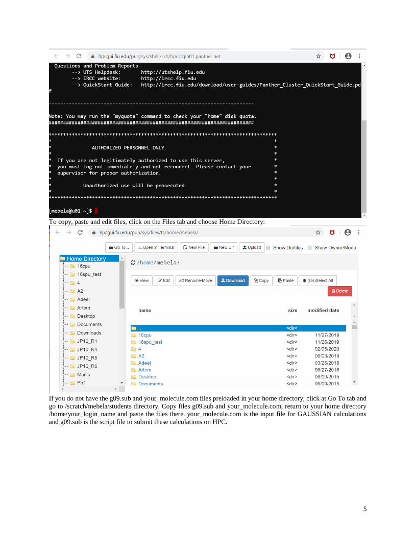
To copy, paste and edit files, click on the Files tab and choose Home Directory:

If you do not have the g09.sub and your_molecule.com files preloaded in your home directory, click at Go To tab and

go to /scratch/mebela/students directory. Copy files g09.sub and your_molecule.com, return to your home directory

/home/your_login_name and paste the files there. your_molecule.com is the input file for GAUSSIAN calculations

and g09.sub is the script file to submit these calculations on HPC.

6

Appendix 2: Description of the GAUSSIAN input file

# b3lyp/6-31G* opt freq !Route Section

!Blank line

Geometry optimization and frequencies for LiH !Title Section

!Blank line

0 1 !Charge and Multiplicity

Li !Molecule Specification

H 1 R

!Blank line

R=1.30

!Blank line

Make sure to include the blank line in the end. After revising the file you can rename it to a name of your choice.

Route section specifies the method and the type of calculations. The method is a quantum chemical procedure

to be used to find an approximate solution for the electronic Schrödinger equation and the basis set for

molecular wave function. The calculations should be carried out employing the density functional B3LYP

method with the 6-31G* basis set (or 6-31G** if your molecule contains an H atom). In density functional

theory (DFT), the electronic energy is expressed as a functional of electron density (square of the wave

function). This group of methods is the most popular and fast developing in quantum chemistry in recent years;

they take into account electronic correlation but are as time-efficient as the Hartree-Fock method.

The basis set is specified after the ‘/’. The need to have a basis set in the GAUSSIAN calculations is related to

the fact that the wave function for each electron in the molecule is expressed as a linear combination of atomic

orbitals, i.e. the orbitals of the hydrogen-atom type. The basis set specifies how many hydrogen-atom type s, p,

d, etc., orbitals are included.

The type of calculations is also specified in the route section with keywords ‘opt’ and ‘freq’. The ‘opt’ keyword

means ‘optimization’; the program is requested to optimize molecular geometry, i.e., to find the structure with

the lowest potential energy. The ‘freq’ keyword specifies calculations of vibrational frequencies. When single-

point calculations are carried out, the ‘opt’ and ‘freq’ commands should not be included and the route section

should look simply as

# b3lyp/6-31G*

The above line will be also used in the calculation of a separate atom since an atom does not have a ‘geometry’

to optimize, neither it has vibrational frequencies.

The route section for a potential energy scan is

# b3lyp/6-31G* opt=modredundant

and the variable for the scan (the interatomic distance) will be defined in a special way shown below.

The title section includes an arbitrary comment describing your calculations. It will be also found in the output

(log) file.

The charge and multiplicity section indicates molecular charge and multiplicity. For the neutral molecules, the

charge is specified as ‘0’. The multiplicity is the number of unpaired electrons in the molecule + 1, i.e., ‘1’ for

singlet, ‘2’ for doublet, ‘3’ for triplet, etc. Neutral atoms have zero charge and the multiplicity is determined by

their electronic structure, i.e, by the number of unpaired electrons.

The molecular specification section is used to input initial molecular geometry. It is specified in the form of

atomic Cartesian coordinates or a so-called z-matrix, which shows interatomic distances, bond angles, and

torsional angles. In the case of a diatomic molecule, students need to specify only the two atoms comprising the

molecule and the distance between them:

Li

H 1 R

7

Here, the first atom in the molecule is lithium ‘Li’ and the second is hydrogen ‘H’ The atomic specification will

include only one line with an atomic symbol. The Li-H distance is designated with the variable ‘R’, which will

be optimized during the calculations. The initial value for this variable is given (in angstrom) after a blank line:

R = 1.30

Make sure to include the blank line in the end!

For the potential energy scan calculations the variable is defined in the following way:

R = 0.5

1 2 s 17 0.1

Here, ‘0.5’ is the initial value of the variable, ‘1 2 s’ means that the distance between atoms 1 and 2 will be

scanned, ‘17’ is the number of steps in the scan calculation and ‘0.1’ is the step size. Make sure to separate the

two lines by a blank line and to include the blank line in the end!

Appendix 3: Description of the submission file for the Gaussian input file

#!/bin/bash

#SBATCH --qos pq_chm3411l

#SBATCH --account acc_chm3411l

#SBATCH -N 1

#SBATCH --cpus-per-task=1

#SBATCH --job-name=test_gaussian

#SBATCH --output=out_%j.log

. $MODULESHOME/../global/profile.modules

module load gaussian/09

export OMP_NUM_THREADS=$SLURM_CPUS_ON_NODE

pwd; hostname; date

echo "Running program on $SLURM_CPUS_ON_NODE CPU cores"

g09 your_molecule.com

date

When submitting different GAUSSIAN calculations the only thing you need to change every time is the name of

your GAUSSIAN input file shown in in bold above.

To submit your GAUSSIAN calculation using the terminal window type

sbatch g09.sub

To check the status of your running or pending jobs and their job ID number (JOBID) type

squeue –u your_login_name

When the calculation is completed, the job disappears from the list. Once the job is running, the output file

“your_molecule.log” with the calculation results is formed in your directory. You can browse this file using the Files

window.

To kill a running job type

scancel JOBID

8

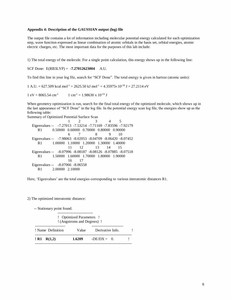
Appendix 4: Description of the GAUSSIAN output (log) file

The output file contains a lot of information including molecular potential energy calculated for each optimization

step, wave function expressed as linear combination of atomic orbitals in the basis set, orbital energies, atomic

electric charges, etc. The most important data for the purposes of this lab include:

1) The total energy of the molecule. For a single point calculation, this energy shows up in the following line:

SCF Done: E(RB3LYP) = -7.27012623004 A.U.

To find this line in your log file, search for “SCF Done”. The total energy is given in hartree (atomic units):

1 A.U. = 627.509 kcal mol-1 = 2625.50 kJ mol-1 = 4.3597510-18 J = 27.2114 eV

1 eV = 8065.54 cm-1 1 cm-1 = 1.98630 x 10-23 J

When geometry optimization is run, search for the final total energy of the optimized molecule, which shows up in

the last appearance of “SCF Done” in the log file. In the potential energy scan log file, the energies show up as the

following table:

Summary of Optimized Potential Surface Scan

1 2 3 4 5

Eigenvalues -- -7.27013 -7.53214 -7.71169 -7.83596 -7.92179

R1 0.50000 0.60000 0.70000 0.80000 0.90000

6 7 8 9 10

Eigenvalues -- -7.98063 -8.02053 -8.04709 -8.06420 -8.07452

R1 1.00000 1.10000 1.20000 1.30000 1.40000

11 12 13 14 15

Eigenvalues -- -8.07996 -8.08187 -8.08126 -8.07885 -8.07518

R1 1.50000 1.60000 1.70000 1.80000 1.90000

16 17

Eigenvalues -- -8.07066 -8.06558

R1 2.00000 2.10000

Here, ‘Eigenvalues’ are the total energies corresponding to various interatomic distances R1.

2) The optimized interatomic distance:

-- Stationary point found.

----------------------------

! Optimized Parameters !

! (Angstroms and Degrees) !

------------------------ -------------------------

! Name Definition Value Derivative Info. !

-----------------------------------------------------------------------------

! R1 R(1,2) 1.6209 -DE/DX = 0. !

-----------------------------------------------------------------------------

9

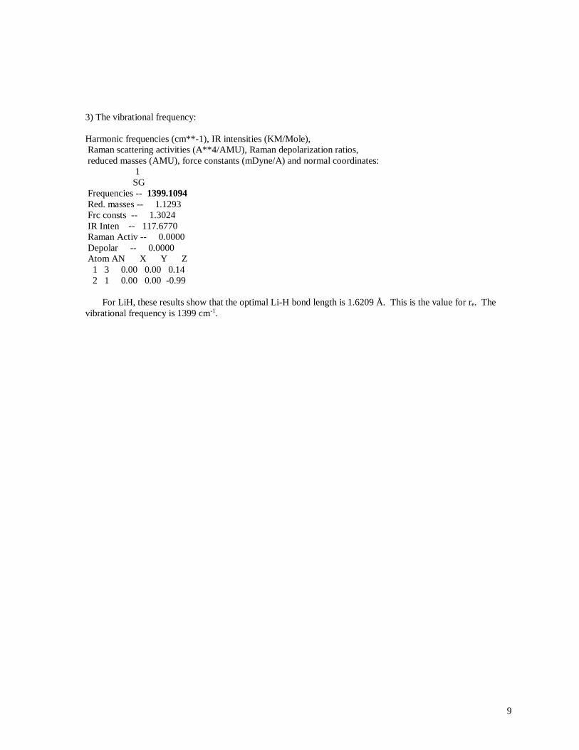
3) The vibrational frequency:

Harmonic frequencies (cm**-1), IR intensities (KM/Mole),

Raman scattering activities (A**4/AMU), Raman depolarization ratios,

reduced masses (AMU), force constants (mDyne/A) and normal coordinates:

1

SG

Frequencies -- 1399.1094

Red. masses -- 1.1293

Frc consts -- 1.3024

IR Inten -- 117.6770

Raman Activ -- 0.0000

Depolar -- 0.0000

Atom AN X Y Z

1 3 0.00 0.00 0.14

2 1 0.00 0.00 -0.99

For LiH, these results show that the optimal Li-H bond length is 1.6209 Å. This is the value for re. The

vibrational frequency is 1399 cm-1.

10

Appendix 5. Alternative ways to access FIU’s HPC cluster

If the remote terminal access (hpcgui.fiu.edu) is not available for some reason, you can install and use other

apps in its stead. Terminal app on Mac and PuTTY on PC can be used in place of the remote terminal ‘Panther Shell

Access” window.

If PuTTY is not preinstalled on your computer (PC) download and install PuTTY from the web. If you are

using a Mac, the Terminal app is included in your system and you do not need to install or use PuTTY.

Click at the PuTTY icon to connect with HPC. Type hpclogin01.fiu.edu as the host name and click at the “Open”

tab:

Enter you FIU accounts login and password:

11

Your connection with HPC is now established and you will be able to submit your GAUSSIAN calculations when

the input and submission files are ready.

If not preinstalled on your PC, download and install WinSCP (an SFTP client for file transfers) from the

web. A convenient SFTP client for Mac users is Cyberduck. WinSCP or Cyberduck will be used instead of the Files

window of the remote terminal access.

Click at the WinSCP icon to connect with HPC. Type hpclogin01.fiu.edu as the host name, enter your login and

password and then login:

12

Now you can access file both on your PC (left) and on HPC (right). You can edit the files and copy them

from your computer to HPC and vice versa by dragging them from left to right or from right to left:

Sample GAUSSIAN input file ‘your_molecule.com’ and GAUSSIAN submission file ‘g09.sub’ are placed in the

HPC directory /scratch/mebela/students. To access them, click on the right hand side of your WinSCP screen, type

ctrl+O, and open the /scratch/mebela/students directory:

13

Copy the files to your PC and revise them as required according to your molecule (see below). When the files are

ready, open your home directory on HPC:

14

Copy the revised files from your PC to your home directory on HPC.

Submit your calculation using the PuTTY window:

Once the job is running, the output file “your_molecule.log” is formed in your directory with the calculation results.

You can browse this file through the WinSCP window. As the calculations are completed, open the output file by

double-clicking on it in WinSCP.