Calculation of Areal Reduction Factors Using NEXRAD ... · CALCULATION OF AREAL REDUCTION FACTORS...

Technical Report Documentation . Report No. FHWA/TX-07/0-4642-3

2. Government Accession No.

3. Recipient's Catalog No. 5. Report Date October 2005 Published: November 2006

4. Title and Subtitle CALCULATION OF AREAL REDUCTION FACTORS USING NEXRAD PRECIPITATION ESTIMATES

6. Performing Organization Code

7. Author(s) Francisco Olivera, Dongkyun Kim, Janghwoan Choi and Ming-Han Li

8. Performing Organization Report No. Report 0-4642-3 10. Work Unit No. (TRAIS)

9. Performing Organization Name and Address Texas Transportation Institute The Texas A&M University System College Station, Texas 77843-3135

11. Contract or Grant No. Project 0-4642 13. Type of Report and Period Covered Technical Report: September 2003 - August 2005

12. Sponsoring Agency Name and Address Texas Department of Transportation Research and Technology Implementation Office P.O. Box 5080 Austin, Texas 78763-5080

14. Sponsoring Agency Code

15. Supplementary Notes Project performed in cooperation with the Texas Department of Transportation and the Federal Highway Administration. Project Title: GIS Static Storm Model Development URL: http://tti.tamu.edu/document/0-4642-3.pdf 16. Abstract In general, larger catchments are less likely than smaller catchments to experience high intensity storms over the whole of the catchment area. Therefore, the conversion of point precipitation into area-averaged precipitation is necessary whenever an area, large enough for rainfall not to be uniform, is to be modeled. However, while point precipitation has been well recorded because of the availability of rain gauge data, areal precipitation cannot be measured, and its estimation has been a subject of research for the last decades. With the understanding that the Next Generation Radar (NEXRAD) precipitation data distributed by the U.S. National Weather Service (NWS) are the best data with spatial coverage available for large areas, this report addresses the estimation of areal reduction factors (ARFs) using this type of data. The study site is the 685,000-km2 area of the state of Texas. Storms were assumed to be elliptically shaped of different aspect ratios and orientations. It was found that, in addition to the storm duration and area already considered in previous studies, ARFs depend also on the geographic region and the precipitation depth, which is associated with the storm frequency for a given duration. Researchers also studied storm shape and orientation. 17. Key Words Precipitation, Areal Reduction Factors, Geographic Information Systems (GIS), NEXRAD Precipitation Estimates, Texas

18. Distribution Statement No restrictions. This document is available to the public through NTIS: National Technical Information Service Springfield, Virginia 22161 http://www.ntis.gov

19. Security Classif.(of this report) Unclassified

20. Security Classif.(of this page) Unclassified

21. No. of Pages 84

22. Price

Form DOT F 1700.7 (8-72) Reproduction of completed page authorized

http://tti.tamu.edu/document/0-4642-3.pdf

http://www.ntis.gov

CALCULATION OF AREAL REDUCTION FACTORS USING NEXRAD PRECIPITATION ESTIMATES

by

Francisco Olivera, Ph.D., P.E. Assistant Professor

Department of Civil Engineering

Dongkyun Kim Graduate Assistant – Research


Janghwoan Choi Graduate Assistant – Research


and

Ming-Han Li, Ph.D. Assistant Professor

Department of Landscape Architecture and Urban Planning

Report 0-4642-3 Project 0-4642

Project Title: GIS Static Storm Model Development

Performed in cooperation with the Texas Department of Transportation

and the Federal Highway Administration

October 2005 Published: November 2006

TEXAS TRANSPORTATION INSTITUTE The Texas A&M University System College Station, Texas 77843-3135

v

DISCLAIMER

This research was performed in cooperation with the Texas Department of Transportation

(TxDOT) and the Federal Highway Administration (FHWA). The contents of this report reflect

the views of the authors, who are responsible for the facts and the accuracy of the data presented

herein. The contents do not necessarily reflect the official view or policies of the FHWA or

TxDOT. This report does not constitute a standard, specification, or regulation.

This report is not intended for construction, bidding, or permits purposes. The engineer in

charge of the project was Francisco Olivera, P.E. #88213.

The United States Government and the State of Texas do not endorse products or

manufacturers. Trade or manufacturers’ names appear herein solely because they are considered

essential to the object of this report.

vi

ACKNOWLEDGMENTS

This project was conducted in cooperation with TxDOT and FHWA.

The authors would like to thank Project Director Rose Marie Klee, Project Coordinator

David Stolpa, and Project Advisors Tedd Carter, George Herrmann, Amy Ronnfeldt, Jaime

Villena-Morales and David Zwernemann for their input and support during this project.

vii

TABLE OF CONTENTS

Page List of Figures............................................................................................................................. viii List of Tables ................................................................................................................................. x 1. Introduction............................................................................................................................... 1 2. Precipitation Data ..................................................................................................................... 7 3. Methodology ............................................................................................................................ 13 4. Results and Analysis ............................................................................................................... 17 5. ArcGIS_Storm Documentation ............................................................................................. 35 6. Moving Storms ........................................................................................................................ 61 7. Conclusions.............................................................................................................................. 69 8. References................................................................................................................................ 71

viii

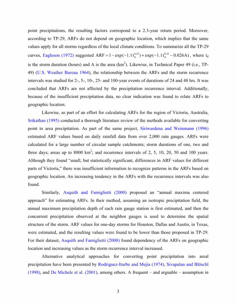
LIST OF FIGURES Page Figure 2.1: Texas WSR-88D Radars (Source: U.S. National Weather Service,

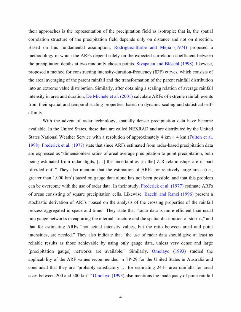
http://www.roc.noaa.gov/interactive/defaultIE.asp). .............................................................. 8 Figure 2.2: Scanning Domain of the Radars within and around Texas. Red Points: Radar

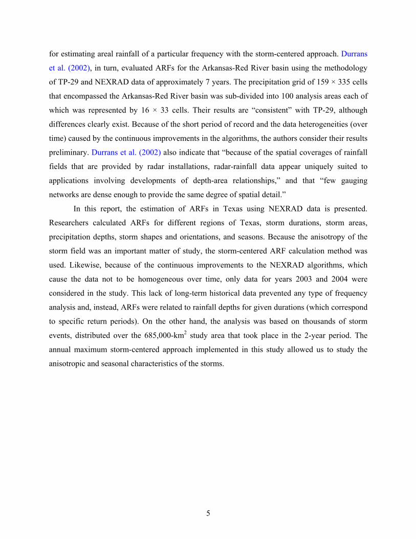
Locations; Blue Area: Radar Scanning Domain; and Black Outline: Texas Border.............. 8 Figure 2.3: Area Served by the West Gulf River Forecasting Center (Purple) and HRAP

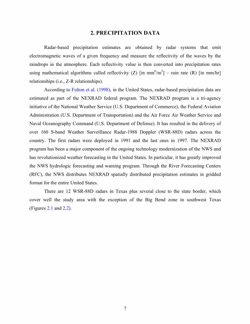
Grid Extent in Which the Data Are Distributed (Green). ..................................................... 11 Figure 3.1: West Gulf River Forecasting Center HRAP Grid. ..................................................... 13 Figure 3.2: 50 km Buffer around Texas........................................................................................ 13 Figure 3.3: 1-hr Duration Concurrent Precipitation Field for June 4, 2003, at 6:00 am.

The Color of Each Cell Represents the Precipitation Depth. Red Cells Have Higher Precipitation Depth than the Blue Ones................................................................................ 14

Figure 3.4: Location of the Cells for Which ARFs Were Calculated for a Storm Duration of 1 hr and Using Stage III Data of 2003.............................................................................. 15

Figure 3.5: Ellipses of Different Areas Shown on a Precipitation Field. Each Ellipse Has Its Own Aspect and Inclination Angle.................................................................................. 16

Figure 4.1: Effect of Location on the ARF Values....................................................................... 17 Figure 4.2: Effect of Precipitation Depth on the ARF Values...................................................... 18 Figure 4.3: Regions of Texas (U.S. Geological Survey 1998). .................................................... 18 Figure 4.4: ARF-Area Plot for Region 4 and Storm Duration of 24. Note the Scatter

of the Points around the Mean Line, Which Is Presumed to Be Caused by the Differences in Precipitation Depth........................................................................................ 19

Figure 4.5: ARF-Area Plot for Region 4 and Duration of 24 hrs. ................................................ 26 Figure 4.6: ARF-Area Plot for Region 4, Duration of 24 hrs and Depth between 64 mm

and 102 mm........................................................................................................................... 26 Figure 4.7a: Normalized Histograms of Aspect for a Duration of 1 hr. ....................................... 27 Figure 4.7b: Normalized Histograms of Aspect for a Duration of 3 hrs. ..................................... 28 Figure 4.7c: Normalized Histograms of Aspect for a Duration of 6 hrs....................................... 28 Figure 4.7d: Normalized Histograms of Aspect for a Duration of 12 hrs. ................................... 29 Figure 4.7e: Normalized Histograms of Aspect for a Duration of 24 hrs..................................... 29 Figure 4.8a: Normalized Histograms of Angle for a Duration of 1 hr. ........................................ 30 Figure 4.8b: Normalized Histograms of Angle for a Duration of 3 hrs........................................ 30 Figure 4.8c: Normalized Histograms of Angle for a Duration of 6 hrs. ....................................... 31 Figure 4.8d: Normalized Histograms of Angle for a Duration of 12 hrs...................................... 31 Figure 4.8e: Normalized Histograms of Angle for a Duration of 24 hrs. ..................................... 32 Figure 4.9: Comparison of ARF-Area Curves According to Different Studies. .......................... 33 Figure 5.1: ArcGIS_Storm Toolbar. ............................................................................................. 35 Figure 5.2: Project Working Directory Menu............................................................................... 35 Figure 5.3: The Project Set Up Window....................................................................................... 36 Figure 5.4: Project Folder Window. ............................................................................................. 36 Figure 5.5: Climate Region Frame. .............................................................................................. 36 Figure 5.6: Open Feature Class of Climate Region for Texas...................................................... 37 Figure 5.7: Select Watersheds Menu. ........................................................................................... 37 Figure 5.8: Select Watersheds Window........................................................................................ 38

ix

Figure 5.9: Example of Selecting Watersheds.............................................................................. 38 Figure 5.10: Hypothetical Storm Menu. ....................................................................................... 39 Figure 5.11: Hypothetical/FHS Menu........................................................................................... 40 Figure 5.12: Input Storm Properties Window............................................................................... 40 Figure 5.13: Storm Properties Window. ....................................................................................... 41 Figure 5.14: IDF Curves Window. ............................................................................................... 41 Figure 5.15: Edit IDF Curves Window......................................................................................... 42 Figure 5.16: Edit Durations Window............................................................................................ 43 Figure 5.17: Edit Isohyet Area Window. ...................................................................................... 44 Figure 5.18: Develop Storm Menu. .............................................................................................. 44 Figure 5.19: Developing Storm Window...................................................................................... 45 Figure 5.20: Symbology Setup. .................................................................................................... 45 Figure 5.21: Storm Feature Class Table. ...................................................................................... 46 Figure 5.22: PMP Menu................................................................................................................ 47 Figure 5.23: PMP Project Setup Menu. ........................................................................................ 47 Figure 5.24: PMP Project Setup Window..................................................................................... 48 Figure 5.25: Location of the HMR52 Executable File. ................................................................ 48 Figure 5.26: Location of the PMP Geodatabase. .......................................................................... 49 Figure 5.27: Input and Output File for HMR52............................................................................ 49 Figure 5.28: Prepare Storm Inputs Menu...................................................................................... 50 Figure 5.29: Input Data Window. ................................................................................................. 50 Figure 5.30: Edit Durations Window............................................................................................ 52 Figure 5.31: Edit Isohyet Areas Window. .................................................................................... 53 Figure 5.32: Basin Table............................................................................................................... 53 Figure 5.33: Run HMR52 Menu................................................................................................... 54 Figure 5.34: Execute HMR52 Window. ....................................................................................... 55 Figure 5.35: HMR52 DOS Window. ............................................................................................ 55 Figure 5.36: Develop Storm Menu. .............................................................................................. 56 Figure 5.37: Developing Storm Window...................................................................................... 56 Figure 5.38: PMP Storm. .............................................................................................................. 57 Figure 5.39: PMP Storm Table. .................................................................................................... 58 Figure 5.40: Modified PMP Menu................................................................................................ 58 Figure 5.41: Animation Toolbar. .................................................................................................. 59 Figure 5.42: Animation Setup Window. ....................................................................................... 59 Figure 6.1: Aspects of Frontal Rainstorms (Mellor 1996)............................................................ 62 Figure 6.2: Storm Analysis. .......................................................................................................... 63 Figure 6.3: Image Process by the Sobel Method. ......................................................................... 64 Figure 6.4: Image Process by Eliminating Noise.......................................................................... 64 Figure 6.5: Image Process Using the Canny Algorithm. .............................................................. 65 Figure 6.6: Segmentation by a Contour Line................................................................................ 65 Figure 6.7: Labeled Objects.......................................................................................................... 66 Figure 6.8: Mesoscale Convective Systems or Rain Bands (Longest Dimension > 100 km). ..... 66 Figure 6.9: Multicell Storms or Rain Cluster (Longest Dimension < 100 km). ........................... 67 Figure 6.10: Rain Cells (Longest Dimension ≈ 5 km).................................................................. 67 Figure 6.11: Storm Data Model. ................................................................................................... 68

x

LIST OF TABLES Page Table 3.1: Number of Cells for Which ARFs Were Calculated. .................................................. 15 Table 4.1: a, b and c for a Duration of 1 hr................................................................................... 21 Table 4.2: a, b and c for a Duration of 3 hrs. ................................................................................ 22 Table 4.3: a, b and c for a Duration of 6 hrs. ................................................................................ 23 Table 4.4: a, b and c for a Duration of 12 hrs. .............................................................................. 24 Table 4.5: a, b and c for a Duration of 24 hrs. .............................................................................. 25

1

1. INTRODUCTION

In general, “larger catchments are less likely than smaller catchments to experience high

intensity storms over the whole of the catchment area” (Siriwardena and Weinmann 1996).

Therefore, the conversion of point precipitation into area-averaged precipitation is necessary

whenever an area, large enough for rainfall not to be uniform, is to be modeled. However, while

point precipitation has been well studied because of the availability of rain gauge data, areal

precipitation cannot be measured, and its estimation has been a subject of research for the last

few decades (U.S. Weather Bureau 1957, 1958a, 1958b, 1959, 1960, 1964; Rodriguez-Iturbe and

Mejia 1974; Frederick et al. 1977; Omolayo 1993; Srikathan 1995; Bacchi and Ranzi 1996;

Siriwardena and Weinmann 1996; Sivapalan and Blöschl 1998; Asquith and Famiglietti 2000;

De Michele et al. 2001; Durrans et al. 2002). This report discusses the estimation of the ratios of

areal average precipitation to point precipitation – also called areal reduction factors (ARFs) –

using radar precipitation data. The study site is the 685,000-km2 area covered by the state of

Texas in the United States.

With the understanding that the Next Generation Radar (NEXRAD) data, the radar

precipitation data distributed by the United States National Weather Service (NWS), are the best

data with areal coverage in Texas, this report addresses the conversion of point precipitation into

areal precipitation using these radar data. It was found that, in addition to the storm duration and

area already considered in previous studies, ARFs depend on the precipitation depth and region

where the event takes place.

A number of approaches for converting point precipitation into areal precipitation are

based on observed precipitation data. Traditionally, ARF-estimation algorithms have been

grouped under two broad categories: those based on geographically fixed rain gauge networks

(known as geographically fixed ARFs) and those based on individual storm events (known as

storm-centered ARFs) (Srikathan 1995). The geographically fixed approach is particularly suited

for using discrete (i.e., point) precipitation data, and ARFs are calculated using data of rain

gauge networks. ARFs are calculated as the ratio of a representative precipitation depth over the

area covered by the network to a (not necessarily concurrent) representative point precipitation

depth. How to estimate the area covered by the network, the representative precipitation depth

over the area, or the representative point precipitation depth, however, changes from method to

method. Moreover, based on the algorithms used to calculate geographically fixed ARFs, it can

2

be said that they are sensitive to the configuration of the network (i.e., adding or removing a rain

gauge can affect the ARF values), and that they do not consider concurrent precipitation depths

(i.e., the areal and point precipitation do not correspond necessarily to the same event). The

storm-centered approach, on the other hand, is well suited for using continuous (i.e., surface)

precipitation data, such as radar data. In this case, ARFs are calculated for individual events for

which they describe their areal properties, and are equal to the ratio of the average precipitation

depth over an area to the concurrent point precipitation depth in the storm center. Because storm-

centered ARFs are estimated for individual events, they can capture the anisotropy of the rainfall

field (i.e., the storm shape and orientation) and the seasonal effect of the atmospheric processes.

The storm-centered approach, however, has the disadvantage that the ARFs are “applicable to

specific types of storm events” (Srikathan 1995), and, therefore, unless a large sample of storm-

centered ARF values are estimated, the main and seasonal trends in the area might not be

captured. In general, it can be observed that while geographically fixed ARFs are the result of

statistically processing precipitation data and then calculating ARF values, storm-centered ARFs

are the result of calculating ARF values for each of a large sample of storms and then statistically

processing them. Both approaches have strengths and weaknesses, and, in both cases, the

extrapolation to areas different from those for which the ARFs were derived should be done

carefully. Other approaches for calculating ARFs do exist, which, in a way, indicate the

complexity of the problem.

One of the first attempts at estimating ARFs in the United States was documented in

Technical Paper 29 – Parts 1 to 5, frequently referred to as TP-29 (U.S. Weather Bureau 1957,

1958a, 1958b, 1959, 1960). In TP-29, for the area associated with a precipitation gauge network,

the ARF values are estimated using the equation n n k

j ijj 1 j 1 i 1

ARF k P P= = =

= ∑ ∑∑ , where jP [L] is the

annual maximum areal precipitation in year j, Pij [L] is the annual maximum point precipitation

at gauge i in year j, k is the number of rain gauges in the network, and n is the number of years

considered in the calculations. The area is defined by k circles of diameter equal to the average

gauge spacing. The analysis was conducted for only 20 rain gauge networks – 13 of which were

located in the Midwest and eastern United States, and 7 along the Pacific Coast – and for periods

of record ranging from 5 to 16 years. ARFs for storm durations of 0.5, 1, 3, 6 and 24 hrs and

areas up to approximately 1,000 km2, were estimated. Because of the averaging of the areal and

3

point precipitations, the resulting factors correspond to a 2.3-year return period. Moreover,

according to TP-29, ARFs do not depend on geographic location, which implies that the same

values apply for all storms regardless of the local climate conditions. To summarize all the TP-29

curves, Eagleson (1972) suggested 0.25 0.25d dARF 1 exp( 1.1t ) exp( 1.1t 0.026A)= − − + − − , where td

is the storm duration (hours) and A is the area (km2). Likewise, in Technical Paper 49 (i.e., TP-

49) (U.S. Weather Bureau 1964), the relationship between the ARFs and the storm recurrence

intervals was studied for 2-, 5-, 10-, 25- and 100-year events of durations of 24 and 48 hrs. It was

concluded that ARFs are not affected by the precipitation recurrence interval. Additionally,

because of the insufficient precipitation data, no clear indication was found to relate ARFs to

geographic location.

Likewise, as part of an effort for calculating ARFs for the region of Victoria, Australia,

Srikathan (1995) conducted a thorough literature review of the methods available for converting

point to area precipitation. As part of the same project, Siriwardena and Weinmann (1996)

estimated ARF values based on daily rainfall data from over 2,000 rain gauges. ARFs were

calculated for a large number of circular sample catchments; storm durations of one, two and

three days; areas up to 8000 km2; and recurrence intervals of 2, 5, 10, 20, 50 and 100 years.

Although they found “small, but statistically significant, differences in ARF values for different

parts of Victoria,” there was insufficient information to recognize patterns in the ARFs based on

geographic location. An increasing tendency in the ARFs with the recurrence intervals was also

found.

Similarly, Asquith and Famiglietti (2000) proposed an “annual maxima centered

approach” for estimating ARFs. In their method, assuming an isotropic precipitation field, the

annual maximum precipitation depth of each rain gauge station is first estimated, and then the

concurrent precipitation observed at the neighbor gauges is used to determine the spatial

structure of the storm. ARF values for one-day storms for Houston, Dallas and Austin, in Texas,

were estimated, and the resulting values were found to be lower than those proposed in TP-29.

For their dataset, Asquith and Famiglietti (2000) found dependency of the ARFs on geographic

location and increasing values as the storm recurrence interval increased.

Alternative analytical approaches for converting point precipitation into areal

precipitation have been presented by Rodriguez-Iturbe and Mejia (1974), Sivapalan and Blöschl

(1998), and De Michele et al. (2001), among others. A frequent – and arguable – assumption in

4

their approaches is the representation of the precipitation field as isotropic; that is, the spatial

correlation structure of the precipitation field depends only on distance and not on direction.

Based on this fundamental assumption, Rodriguez-Iturbe and Mejia (1974) proposed a

methodology in which the ARFs depend solely on the expected correlation coefficient between

the precipitation depths at two randomly chosen points. Sivapalan and Blöschl (1998), likewise,

proposed a method for constructing intensity-duration-frequency (IDF) curves, which consists of

the areal averaging of the parent rainfall and the transformation of the parent rainfall distribution

into an extreme value distribution. Similarly, after obtaining a scaling relation of average rainfall

intensity in area and duration, De Michele et al. (2001) calculate ARFs of extreme rainfall events

from their spatial and temporal scaling properties, based on dynamic scaling and statistical self-

affinity.

With the advent of radar technology, spatially denser precipitation data have become

available. In the United States, these data are called NEXRAD and are distributed by the United

States National Weather Service with a resolution of approximately 4 km × 4 km (Fulton et al.

1998). Frederick et al. (1977) state that since ARFs estimated from radar-based precipitation data

are expressed as “dimensionless ratios of areal average precipitation to point precipitation, both

being estimated from radar digits, […] the uncertainties [in the] Z-R relationships are in part

‘divided out’.” They also mention that the estimation of ARFs for relatively large areas (i.e.,

greater than 1,000 km2) based on gauge data alone has not been possible, and that this problem

can be overcome with the use of radar data. In their study, Frederick et al. (1977) estimate ARFs

of areas consisting of square precipitation cells. Likewise, Bacchi and Ranzi (1996) present a

stochastic derivation of ARFs “based on the analysis of the crossing properties of the rainfall

process aggregated in space and time.” They state that “radar data is more efficient than usual

rain gauge networks in capturing the internal structure and the spatial distribution of storms,” and

that for estimating ARFs “not actual intensity values, but the ratio between areal and point

intensities, are needed.” They also indicate that “the use of radar data should give at least as

reliable results as those achievable by using only gauge data, unless very dense and large

[precipitation gauge] networks are available.” Similarly, Omolayo (1993) studied the

applicability of the ARF values recommended in TP-29 for the United States in Australia and

concluded that they are “probably satisfactory … for estimating 24-hr area rainfalls for areal

sizes between 200 and 500 km2.” Omolayo (1993) also mentions the inadequacy of point rainfall

5

for estimating areal rainfall of a particular frequency with the storm-centered approach. Durrans

et al. (2002), in turn, evaluated ARFs for the Arkansas-Red River basin using the methodology

of TP-29 and NEXRAD data of approximately 7 years. The precipitation grid of 159 × 335 cells

that encompassed the Arkansas-Red River basin was sub-divided into 100 analysis areas each of

which was represented by 16 × 33 cells. Their results are “consistent” with TP-29, although

differences clearly exist. Because of the short period of record and the data heterogeneities (over

time) caused by the continuous improvements in the algorithms, the authors consider their results

preliminary. Durrans et al. (2002) also indicate that “because of the spatial coverages of rainfall

fields that are provided by radar installations, radar-rainfall data appear uniquely suited to

applications involving developments of depth-area relationships,” and that “few gauging

networks are dense enough to provide the same degree of spatial detail.”

In this report, the estimation of ARFs in Texas using NEXRAD data is presented.

Researchers calculated ARFs for different regions of Texas, storm durations, storm areas,

precipitation depths, storm shapes and orientations, and seasons. Because the anisotropy of the

storm field was an important matter of study, the storm-centered ARF calculation method was

used. Likewise, because of the continuous improvements to the NEXRAD algorithms, which

cause the data not to be homogeneous over time, only data for years 2003 and 2004 were

considered in the study. This lack of long-term historical data prevented any type of frequency

analysis and, instead, ARFs were related to rainfall depths for given durations (which correspond

to specific return periods). On the other hand, the analysis was based on thousands of storm

events, distributed over the 685,000-km2 study area that took place in the 2-year period. The

annual maximum storm-centered approach implemented in this study allowed us to study the

anisotropic and seasonal characteristics of the storms.

7

2. PRECIPITATION DATA

Radar-based precipitation estimates are obtained by radar systems that emit

electromagnetic waves of a given frequency and measure the reflectivity of the waves by the

raindrops in the atmosphere. Each reflectivity value is then converted into precipitation rates

using mathematical algorithms called reflectivity (Z) [in mm6/m3] – rain rate (R) [in mm/hr]

relationships (i.e., Z-R relationships).

According to Fulton et al. (1998), in the United States, radar-based precipitation data are

estimated as part of the NEXRAD federal program. The NEXRAD program is a tri-agency

initiative of the National Weather Service (U.S. Department of Commerce), the Federal Aviation

Administration (U.S. Department of Transportation) and the Air Force Air Weather Service and

Naval Oceanography Command (U.S. Department of Defense). It has resulted in the delivery of

over 160 S-band Weather Surveillance Radar-1988 Doppler (WSR-88D) radars across the

country. The first radars were deployed in 1991 and the last ones in 1997. The NEXRAD

program has been a major component of the ongoing technology modernization of the NWS and

has revolutionized weather forecasting in the United States. In particular, it has greatly improved

the NWS hydrologic forecasting and warning program. Through the River Forecasting Centers

(RFC), the NWS distributes NEXRAD spatially distributed precipitation estimates in gridded

format for the entire United States.

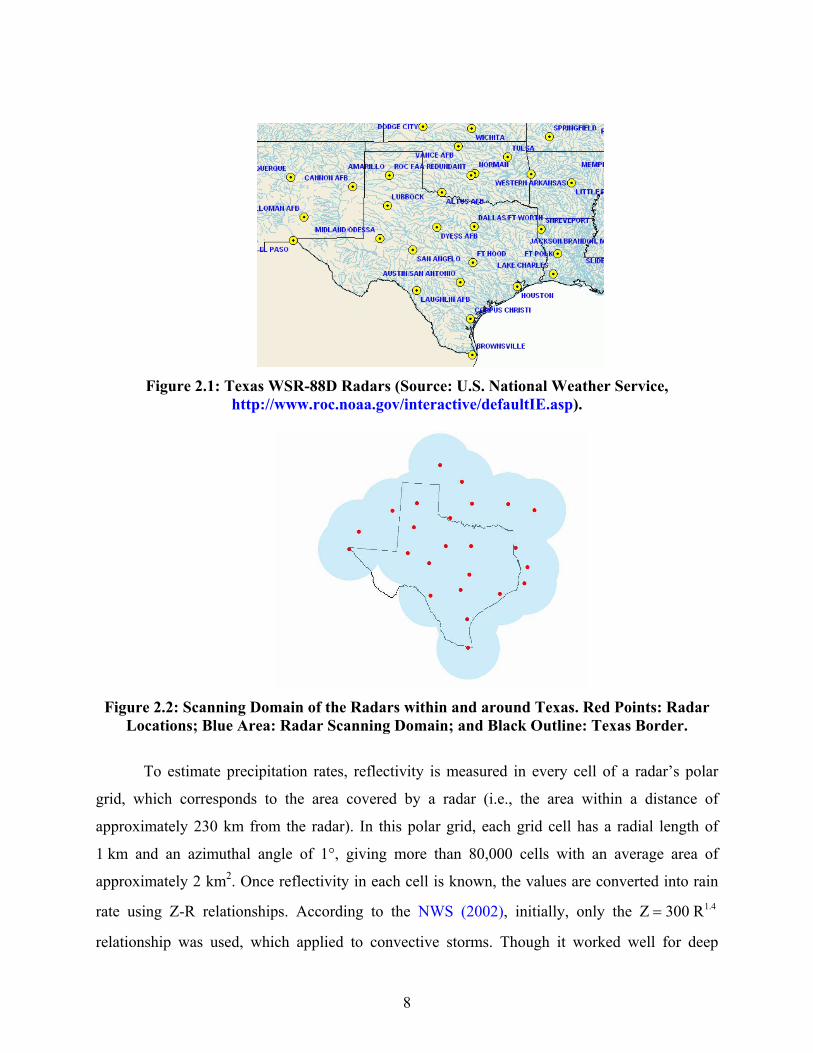
There are 12 WSR-88D radars in Texas plus several close to the state border, which

cover well the study area with the exception of the Big Bend zone in southwest Texas

(Figures 2.1 and 2.2).

8

Figure 2.1: Texas WSR-88D Radars (Source: U.S. National Weather Service,

http://www.roc.noaa.gov/interactive/defaultIE.asp).

Figure 2.2: Scanning Domain of the Radars within and around Texas. Red Points: Radar

Locations; Blue Area: Radar Scanning Domain; and Black Outline: Texas Border.

To estimate precipitation rates, reflectivity is measured in every cell of a radar’s polar

grid, which corresponds to the area covered by a radar (i.e., the area within a distance of

approximately 230 km from the radar). In this polar grid, each grid cell has a radial length of

1 km and an azimuthal angle of 1°, giving more than 80,000 cells with an average area of

approximately 2 km2. Once reflectivity in each cell is known, the values are converted into rain

rate using Z-R relationships. According to the NWS (2002), initially, only the 1.4Z 300 R=

relationship was used, which applied to convective storms. Though it worked well for deep

http://www.roc.noaa.gov/interactive/defaultIE.asp

9

convective precipitation systems, it underestimated, often severely, other types of storms. In

1997, the 1.2Z 250 R= relationship was proposed, which applied to hurricanes, tropical storms

and small scale deep-saturated storms fed by tropical oceanic moisture. Likewise, in 1999, the 1.6Z 200 R= relationship was developed for general stratiform events, and 2.0Z 130 R= and

2.0Z 75 R= for winter stratiform events east and west of the continental divide, respectively.

After estimating the rain rate in every cell, the values obtained for each two consecutive radial

cells are averaged defining a new polar grid in which the cells have a radial length of 2 km and

the same azimuthal angle of 1°. Further corrections are then applied to account for the existence

of hail cores in the thunderstorm clouds, which produce extremely high reflectivities that can be

misinterpreted as unusually high rain rates; abnormal rain rate changes over time in a cell; or

signal degradation from partial beam filling, which may reduce the estimates at far ranges

(Fulton et al. 1998). The hourly digital precipitation array (DPA) is then remapped from the

polar array in which the rain rates are computed onto the Hydrologic Rainfall Analysis Project

(HRAP) grid, which is a grid that covers the conterminous United States. The HRAP grid cell

size ranges from about 3.7 km at southern U.S. latitudes to about 4.4 km at northern U.S.

latitudes. A square HRAP grid of 131 × 131 cells, centered at the radar, covers the 230-km range

domain of the WSR-88D rainfall estimates. The DPA is mapped to this common grid so that it

can be mosaicked with other DPAs across the country in subsequent regional and national

rainfall processing. The resulting hourly precipitation estimates constitute the Stage I NEXRAD

data.

Stage II NEXRAD data provide an optimal estimate of hourly rainfall using a

multivariate objective analysis scheme incorporating both radar and rain gauge observations.

This multisensor estimate of rainfall is performed once per hour for each radar on the HRAP grid

using as input the hourly DPA product from Stage I and all available rain gauge data (Fulton et

al. 1998). First, a uniform mean field gauge–radar bias is applied using a Kalman filter approach.

This adjustment, in the form of a gauge–radar multiplicative bias, is applied uniformly over each

WSR-88D scanning domain and, therefore, is called mean field bias adjustment. Because these

computed hourly biases are representative of the total scanning domain, they do not account for

the spatial variability of the bias within individual storms. Thus, the mean field bias adjustment

is expected to account for spatially uniform radar estimation errors such as hardware

miscalibration, wet radome attenuation and inappropriate Z–R coefficients. Next, a second

10

nonuniform bias is applied, which may vary depending on the range, azimuthal angle, rainfall

type and other factors. To account for the spatial heterogeneity, the rainfall estimates are locally

adjusted using a multivariate optimal estimation procedure that incorporates observed gauge

data. In this estimation procedure, the weights for radar and gauge estimates at each HRAP grid

cell are determined such that their linear combination minimizes the expected error variance of

the estimate. A decreasing (increasing) weight is placed on the gauge (radar) accumulation as the

distance increases away from the gauge. Likewise, Stage III NEXRAD data are obtained by

mosaicking Stage II rainfall estimates from radars with overlapping scanning domains. Finally,

Multisensor Precipitation Estimator (MPE) NEXRAD data take advantage of precipitation values

from satellites in addition to those from radars and rain gauges. Satellite data are of great

importance for filling up the areas that are not covered by radars or rain gauges, such as the Big

Bend area in southwest Texas. With respect to Stage III, MPE also improves the mosaicking and

local bias correction algorithms (Seo 2003). A discussion on the algorithms for adjusting

precipitation estimates to gauge data is presented by Young et al. (2000).

Unavoidably, in the long process that expands from measuring reflectivity to estimating

precipitation depths, different errors can be made (NWS 2002). The vertical profile reflectivity

(VPR) effect, for example, can induce overestimation of reflectivity by a factor of 2 and

underestimation by a factor of 10. The erroneous reflectivity is obtained when the radar detector

samples the electromagnetic waves that hit the raindrops in the freezing level, which is located as

low as 2 km above the ground level in the cold season. The VPR effect is more pronounced in

the areas that are far from the radar. Likewise, the selection of the appropriate Z-R relationship

for the specific rainfall characteristics (i.e., tropical, stratiform or convective) affects the

precipitation estimates. Inconsistent sampling of electromagnetic waves (i.e., number of pulses

per sampling volume, number of scans per hour, beam width, among others) can also affect the

resulting estimates, but it is usually limited to geographically small locations. Finally, even

though the mean field bias adjustment enhances the overall quality of the radar measurement, it

can induce errors at specific locations.

Radar-based precipitation data have been widely used in different hydrologic applications

including rainfall runoff modeling and real-time flood warning systems (Ogden and Julien 1994;

Bedient et al. 2000; Ogden et al. 2000; Smith et al. 2001; Giannoni et al. 2003; Bedient et al.

2003; Vieux and Bedient 2004; Vieux and Vieux 2004; Moon et al. 2004). Notwithstanding the

11

fact that NEXRAD precipitation data are subject to inaccuracies due to a variety of error sources

(NWS 2002), at present, it is the only continuous spatially distributed precipitation database

available countrywide at its resolution.

According to Durrans et al. (2002), “the most significant limitations of radar-rainfall data,

both for frequency analysis and for development of depth-area relationships, are the shortness of

the records and the heterogeneities caused by continual improvements to the data processing

algorithms.” Because of this shortness of the records and data heterogeneities, only data for years

2003 and 2004 were considered in the study. This lack of long-term historical data prevented any

type of frequency analysis and, instead, ARFs were related to rainfall depths for given durations

(which correspond to specific return periods). On the other hand, the analysis was based on more

than 17,500 storm events of different durations that took place in the 2-year period, distributed

over the 685,000-km2 study area. This project used both MPE and Stage III NEXRAD data for

comparison purposes. Since Texas falls completely within the West Gulf River Forecasting

Center (WGRFC) area, the data were obtained for that specific RFC from the NWS website

(NWS 2005). The area served by the WGRFC comprises the drainage area of the Texas Gulf

including the Sabine River and the Rio Grande. The hourly DPA is distributed in HRAP grid

format and covers a much larger area than that served by the WGRFC (Figure 2.3).

Figure 2.3: Area Served by the West Gulf River Forecasting Center (Purple) and HRAP

Grid Extent in Which the Data Are Distributed (Green).

13

3. METHODOLOGY

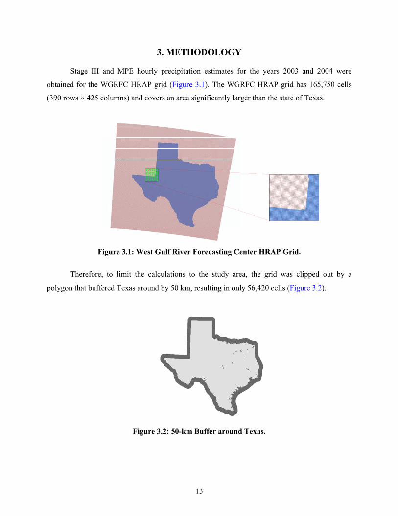
Stage III and MPE hourly precipitation estimates for the years 2003 and 2004 were

obtained for the WGRFC HRAP grid (Figure 3.1). The WGRFC HRAP grid has 165,750 cells

(390 rows × 425 columns) and covers an area significantly larger than the state of Texas.

Figure 3.1: West Gulf River Forecasting Center HRAP Grid.

Therefore, to limit the calculations to the study area, the grid was clipped out by a

polygon that buffered Texas around by 50 km, resulting in only 56,420 cells (Figure 3.2).

Figure 3.2: 50-km Buffer around Texas.

14

For each cell of the clipped grid, the annual maximum precipitation depth was calculated,

and its value was stored along with its corresponding time of occurrence. For durations other

than 1 hr (which is the time step of the original dataset), a moving window over time was defined

so that the annual maximum accounted for the consecutive hours that generated the maximum

depth for the given duration. As a result, grids of annual maxima and date of occurrence for

durations of 1 hr, 3 hrs, 6 hrs, 12 hrs and 24 hrs were generated.

ARF calculations were conducted only for those cells in which: (1) the annual maximum

was greater than a threshold depth value; and (2) the cell value was the greatest in a 21 × 21-cell

square window, centered at the cell, of concurrent precipitation. The threshold values were

20 mm for a storm duration of 1 hr, 25 mm for 3 hrs, 30 mm for 6 hrs, 30 mm for 12 hrs and

40 mm for 24 hrs, and correspond approximately to the 2-year precipitation depth for the given

duration according to TP-40 (U.S. Weather Bureau 1961). The requirement that the cell has to

have the greatest value in the neighborhood is necessary to ensure that the cell is the storm center

(Figure 3.3).

Figure 3.3: 1-hr Duration Concurrent Precipitation Field for June 4, 2003, at 6:00 am. The

Color of Each Cell Represents the Precipitation Depth. Red Cells Have Higher Precipitation Depth than the Blue Ones.

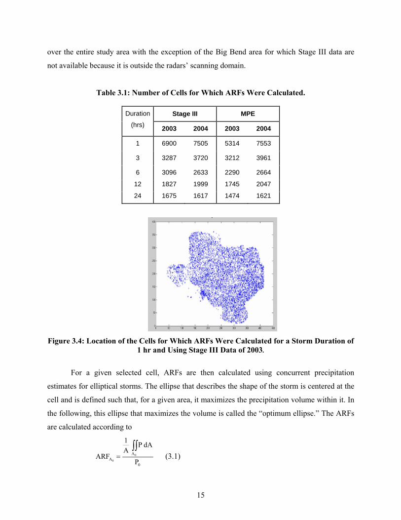
After selecting the cells that satisfy the conditions, ARFs were calculated for these cells

only. Table 3.1 indicates the number of cells for which ARFs were calculated per storm duration,

year and type of NEXRAD data, and Figure 3.4 shows their location for the specific case of a

1-hr duration, year 2003 and Stage III data. In Figure 3.4, note that the cells are well distributed

15

over the entire study area with the exception of the Big Bend area for which Stage III data are

not available because it is outside the radars’ scanning domain.

Table 3.1: Number of Cells for Which ARFs Were Calculated.

Stage III MPE Duration

(hrs) 2003 2004 2003 2004

1 6900 7505 5314 7553

3 3287 3720 3212 3961

6 3096 2633 2290 2664

12 1827 1999 1745 2047

24 1675 1617 1474 1621

Figure 3.4: Location of the Cells for Which ARFs Were Calculated for a Storm Duration of

1 hr and Using Stage III Data of 2003.

For a given selected cell, ARFs are then calculated using concurrent precipitation

estimates for elliptical storms. The ellipse that describes the shape of the storm is centered at the

cell and is defined such that, for a given area, it maximizes the precipitation volume within it. In

the following, this ellipse that maximizes the volume is called the “optimum ellipse.” The ARFs

are calculated according to

0

0

AA

0

1 P dAA

ARFP

=∫∫

(3.1)

16

where 0A

P dA∫∫ [L3] is the precipitation volume in the optimum ellipse A0, A [L2] is the area of

the optimum ellipse A0, P0 is the precipitation at the cell, and ARFA0 is the areal reduction factor

for the cell and area A. Note that there can be several optimum ellipses of different areas

centered at the same cell, thus giving different ARFs for different areas. Note, as well, that all

concurrent precipitation values can be retrieved because the time of occurrence of the cell

maximum was previously stored.

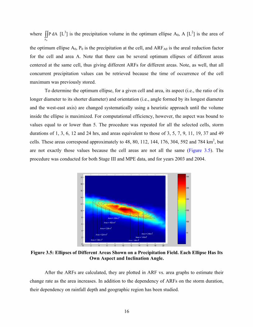
To determine the optimum ellipse, for a given cell and area, its aspect (i.e., the ratio of its

longer diameter to its shorter diameter) and orientation (i.e., angle formed by its longest diameter

and the west-east axis) are changed systematically using a heuristic approach until the volume

inside the ellipse is maximized. For computational efficiency, however, the aspect was bound to

values equal to or lower than 5. The procedure was repeated for all the selected cells, storm

durations of 1, 3, 6, 12 and 24 hrs, and areas equivalent to those of 3, 5, 7, 9, 11, 19, 37 and 49

cells. These areas correspond approximately to 48, 80, 112, 144, 176, 304, 592 and 784 km2, but

are not exactly those values because the cell areas are not all the same (Figure 3.5). The

procedure was conducted for both Stage III and MPE data, and for years 2003 and 2004.

Figure 3.5: Ellipses of Different Areas Shown on a Precipitation Field. Each Ellipse Has Its

Own Aspect and Inclination Angle.

After the ARFs are calculated, they are plotted in ARF vs. area graphs to estimate their

change rate as the area increases. In addition to the dependency of ARFs on the storm duration,

their dependency on rainfall depth and geographic region has been studied.

17

4. RESULTS AND ANALYSIS

The result of the ARF calculation was a 255,048-row and 10-column table, in which each

row corresponded to an ARF calculation and the columns were X-coordinate, Y-coordinate,

storm duration, precipitation depth in the cell, time of occurrence in the year, ellipse area, ellipse

aspect, ellipse orientation, geographic region and areal reduction factor. In the following, and for

the sake of brevity, these variables are referred to as X, Y, duration (td), depth (D), hour (H), area

(A), aspect (ρ), orientation (θ), region and areal reduction factor (ARF). These data were

analyzed to find patterns and relationships between the different variables. As mentioned above,

previous studies show that ARFs decrease with area and increase with duration; however,

noteworthy variability was found also with region and depth (Figures 4.1 and 4.2).

Figure 4.1: Effect of Location on the ARF Values.

18

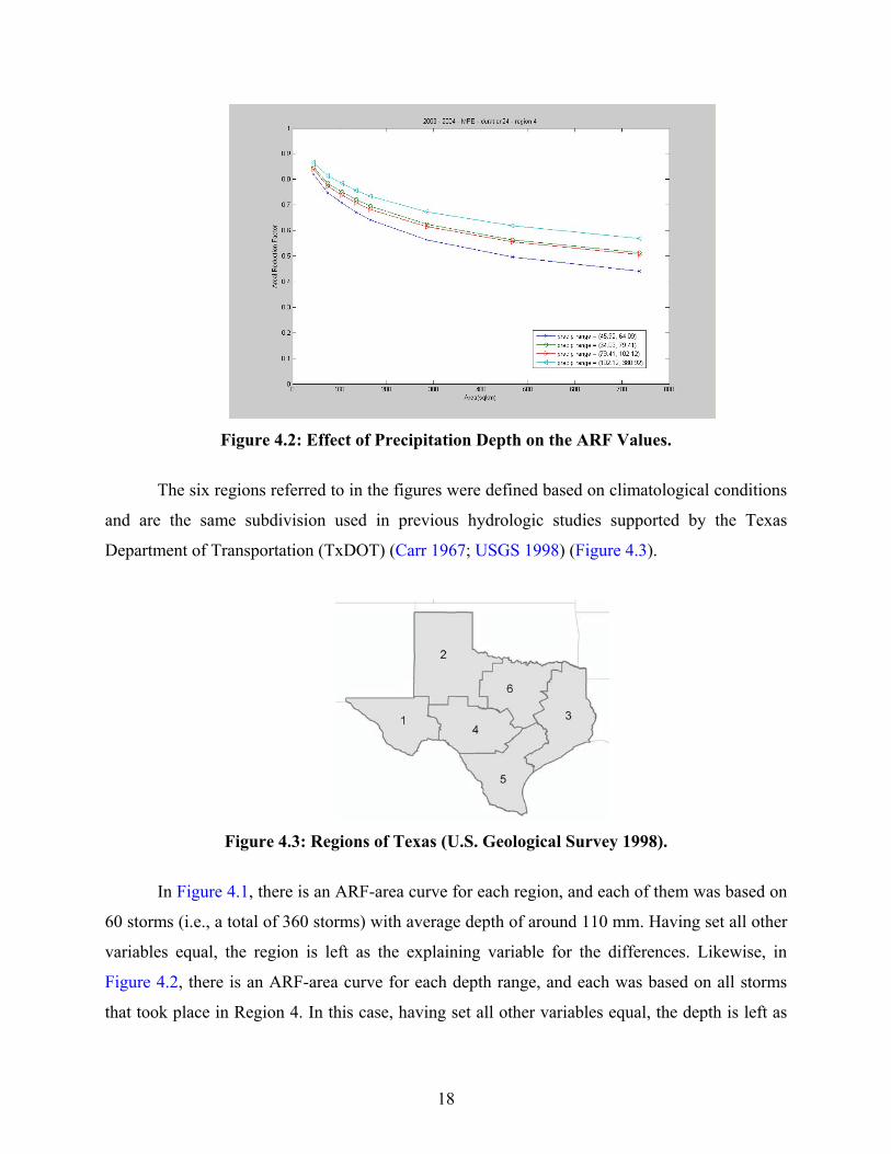
Figure 4.2: Effect of Precipitation Depth on the ARF Values.

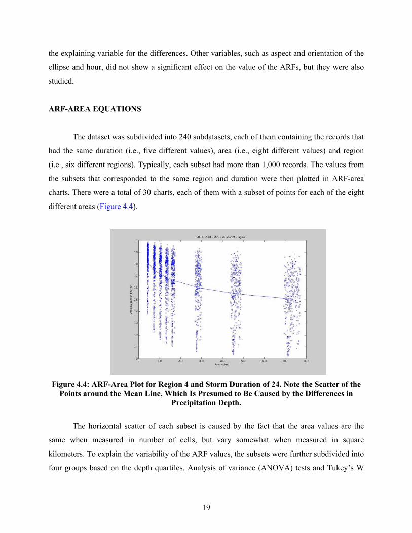
The six regions referred to in the figures were defined based on climatological conditions

and are the same subdivision used in previous hydrologic studies supported by the Texas

Department of Transportation (TxDOT) (Carr 1967; USGS 1998) (Figure 4.3).

Figure 4.3: Regions of Texas (U.S. Geological Survey 1998).

In Figure 4.1, there is an ARF-area curve for each region, and each of them was based on

60 storms (i.e., a total of 360 storms) with average depth of around 110 mm. Having set all other

variables equal, the region is left as the explaining variable for the differences. Likewise, in

Figure 4.2, there is an ARF-area curve for each depth range, and each was based on all storms

that took place in Region 4. In this case, having set all other variables equal, the depth is left as

19

the explaining variable for the differences. Other variables, such as aspect and orientation of the

ellipse and hour, did not show a significant effect on the value of the ARFs, but they were also

studied.

ARF-AREA EQUATIONS

The dataset was subdivided into 240 subdatasets, each of them containing the records that

had the same duration (i.e., five different values), area (i.e., eight different values) and region

(i.e., six different regions). Typically, each subset had more than 1,000 records. The values from

the subsets that corresponded to the same region and duration were then plotted in ARF-area

charts. There were a total of 30 charts, each of them with a subset of points for each of the eight

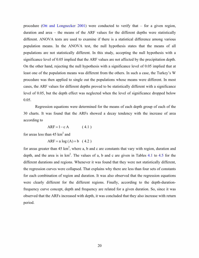
different areas (Figure 4.4).

Figure 4.4: ARF-Area Plot for Region 4 and Storm Duration of 24. Note the Scatter of the

Points around the Mean Line, Which Is Presumed to Be Caused by the Differences in Precipitation Depth.

The horizontal scatter of each subset is caused by the fact that the area values are the

same when measured in number of cells, but vary somewhat when measured in square

kilometers. To explain the variability of the ARF values, the subsets were further subdivided into

four groups based on the depth quartiles. Analysis of variance (ANOVA) tests and Tukey’s W

20

procedure (Ott and Longnecker 2001) were conducted to verify that – for a given region,

duration and area – the means of the ARF values for the different depths were statistically

different. ANOVA tests are used to examine if there is a statistical difference among various

population means. In the ANOVA test, the null hypothesis states that the means of all

populations are not statistically different. In this study, accepting the null hypothesis with a

significance level of 0.05 implied that the ARF values are not affected by the precipitation depth.

On the other hand, rejecting the null hypothesis with a significance level of 0.05 implied that at

least one of the population means was different from the others. In such a case, the Turkey’s W

procedure was then applied to single out the populations whose means were different. In most

cases, the ARF values for different depths proved to be statistically different with a significance

level of 0.05, but the depth effect was neglected when the level of significance dropped below

0.05.

Regression equations were determined for the means of each depth group of each of the

30 charts. It was found that the ARFs showed a decay tendency with the increase of area

according to

ARF 1 c A= − ( 4.1 )

for areas less than 45 km2 and

ARF a log (A) b= + ( 4.2 )

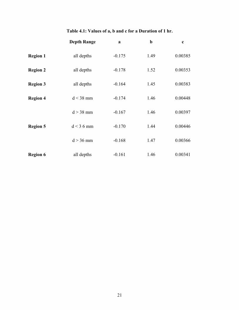
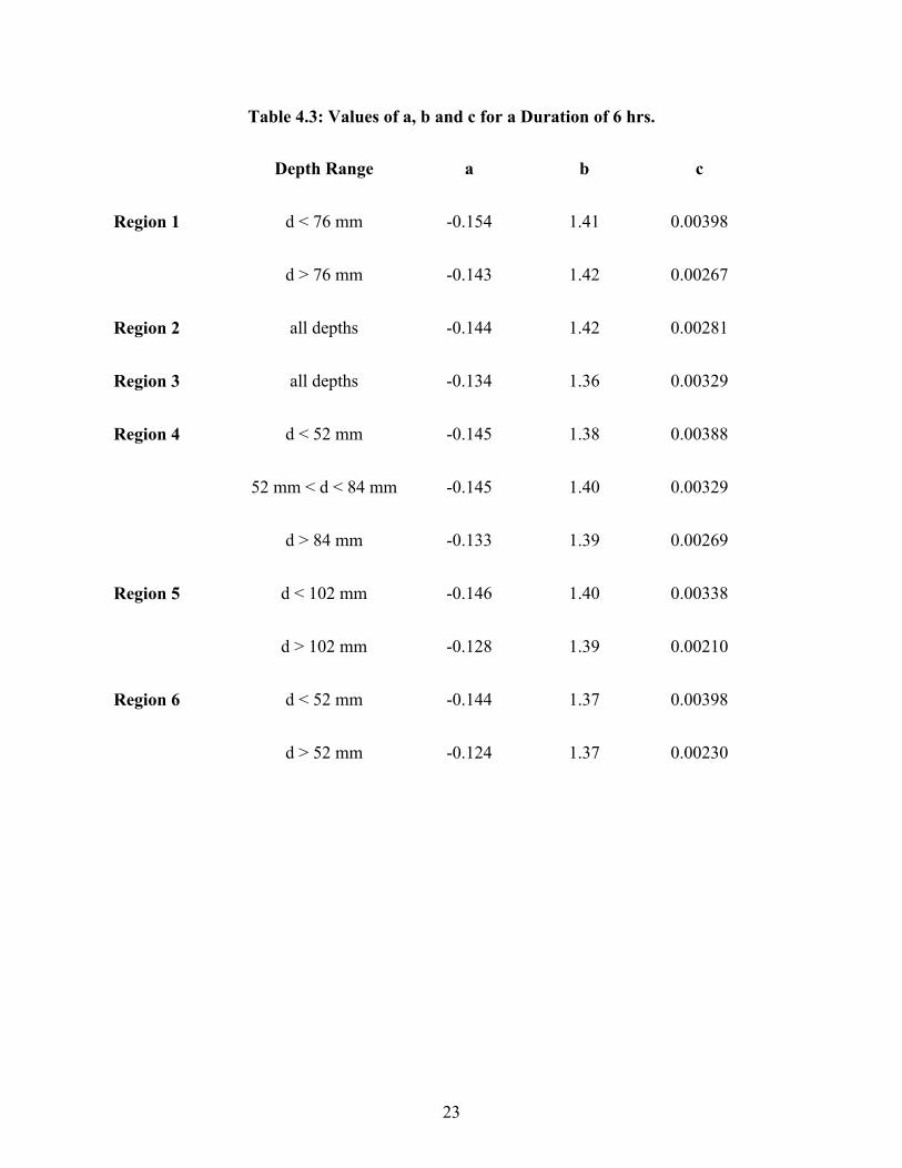
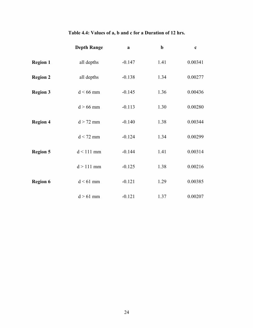
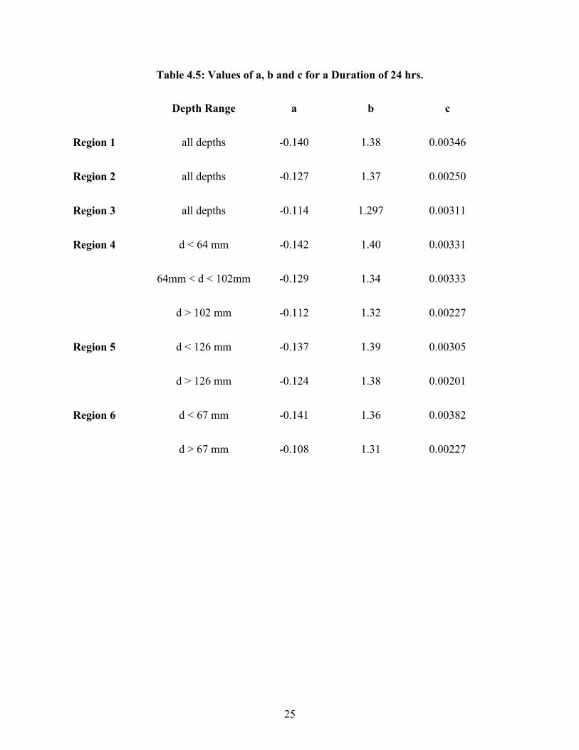
for areas greater than 45 km2, where a, b and c are constants that vary with region, duration and

depth, and the area is in km2. The values of a, b and c are given in Tables 4.1 to 4.5 for the

different durations and regions. Whenever it was found that they were not statistically different,

the regression curves were collapsed. That explains why there are less than four sets of constants

for each combination of region and duration. It was also observed that the regression equations

were clearly different for the different regions. Finally, according to the depth-duration-

frequency curve concept, depth and frequency are related for a given duration. So, since it was

observed that the ARFs increased with depth, it was concluded that they also increase with return

period.

21

Table 4.1: Values of a, b and c for a Duration of 1 hr.

Depth Range a b c

Region 1 all depths -0.175 1.49 0.00385



Region 4 d < 38 mm -0.174 1.46 0.00448

d > 38 mm -0.167 1.46 0.00397

Region 5 d < 3 6 mm -0.170 1.44 0.00446

d > 36 mm -0.168 1.47 0.00366


22

Table 4.2: Values of a, b and c for a Duration of 3 hrs.

Depth Range a b c




Region 4 d < 46 mm -0.157 1.42 0.00393

46 mm < d < 74 mm -0.146 1.39 0.00363

d > 74 mm -0.146 1.43 0.00269

Region 5 d < 66 mm -0.157 1.42 0.00387

d > 66 mm -0.151 1.45 0.00268

Region 6 d < 56 mm -0.132 1.34 0.00353

d > 56 mm -0.135 1.41 0.00244

23


Depth Range a b c

Region 1 d < 76 mm -0.154 1.41 0.00398

d > 76 mm -0.143 1.42 0.00267



Region 4 d < 52 mm -0.145 1.38 0.00388

52 mm < d < 84 mm -0.145 1.40 0.00329

d > 84 mm -0.133 1.39 0.00269

Region 5 d < 102 mm -0.146 1.40 0.00338

d > 102 mm -0.128 1.39 0.00210

Region 6 d < 52 mm -0.144 1.37 0.00398

d > 52 mm -0.124 1.37 0.00230

24


Depth Range a b c



Region 3 d < 66 mm -0.145 1.36 0.00436

d > 66 mm -0.113 1.30 0.00280

Region 4 d > 72 mm -0.140 1.38 0.00344

d < 72 mm -0.124 1.34 0.00299

Region 5 d < 111 mm -0.144 1.41 0.00314

d > 111 mm -0.125 1.38 0.00216

Region 6 d < 61 mm -0.121 1.29 0.00385

d > 61 mm -0.121 1.37 0.00207

25


Depth Range a b c




Region 4 d < 64 mm -0.142 1.40 0.00331

64mm < d < 102mm -0.129 1.34 0.00333

d > 102 mm -0.112 1.32 0.00227

Region 5 d < 126 mm -0.137 1.39 0.00305

d > 126 mm -0.124 1.38 0.00201

Region 6 d < 67 mm -0.141 1.36 0.00382

d > 67 mm -0.108 1.31 0.00227

26

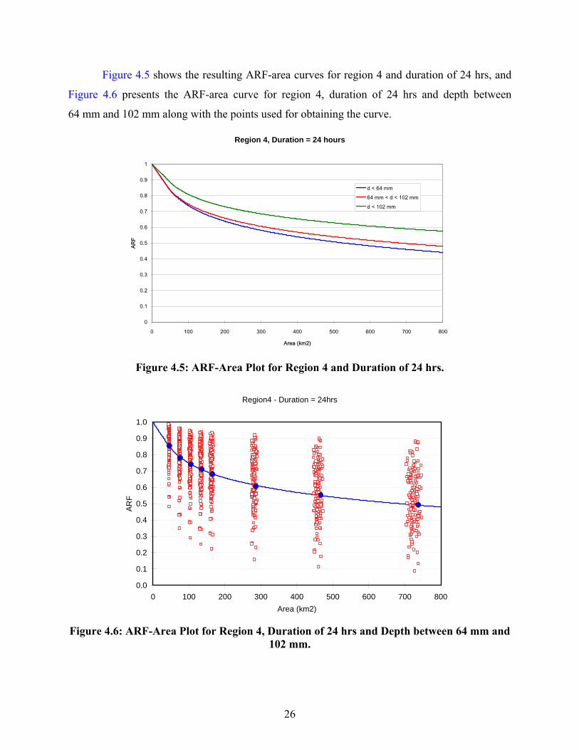
Figure 4.5 shows the resulting ARF-area curves for region 4 and duration of 24 hrs, and

Figure 4.6 presents the ARF-area curve for region 4, duration of 24 hrs and depth between

64 mm and 102 mm along with the points used for obtaining the curve.

Region 4, Duration = 24 hours

0

0.1

0.2

0.3

0.4

0.5

0.6

0.7

0.8

0.9

1

0 100 200 300 400 500 600 700 800

Area (km2)

ARF

d < 64 mm64 mm < d < 102 mmd < 102 mm

Figure 4.5: ARF-Area Plot for Region 4 and Duration of 24 hrs.

Region4 - Duration = 24hrs

0.0

0.1

0.2

0.3

0.4

0.5

0.6

0.7

0.8

0.9

1.0

0 100 200 300 400 500 600 700 800Area (km2)

ARF

Figure 4.6: ARF-Area Plot for Region 4, Duration of 24 hrs and Depth between 64 mm and

102 mm.

27

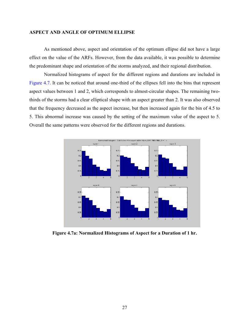
ASPECT AND ANGLE OF OPTIMUM ELLIPSE

As mentioned above, aspect and orientation of the optimum ellipse did not have a large

effect on the value of the ARFs. However, from the data available, it was possible to determine

the predominant shape and orientation of the storms analyzed, and their regional distribution.

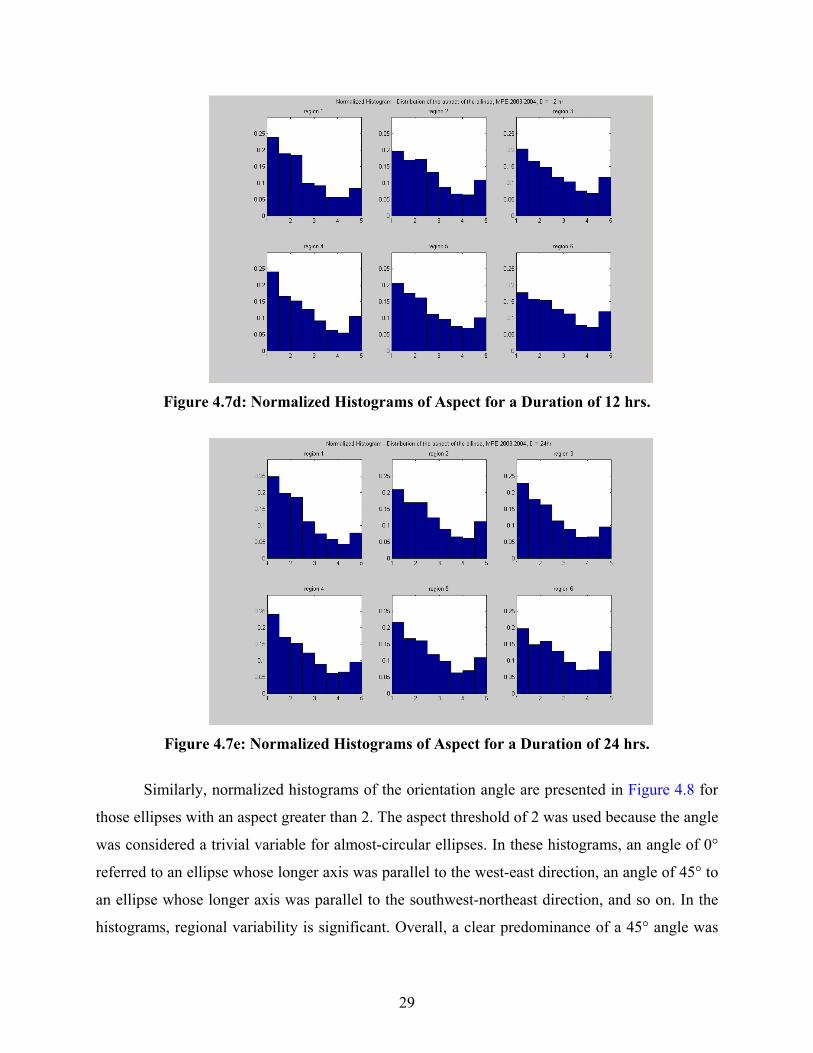
Normalized histograms of aspect for the different regions and durations are included in

Figure 4.7. It can be noticed that around one-third of the ellipses fell into the bins that represent

aspect values between 1 and 2, which corresponds to almost-circular shapes. The remaining two-

thirds of the storms had a clear elliptical shape with an aspect greater than 2. It was also observed

that the frequency decreased as the aspect increase, but then increased again for the bin of 4.5 to

5. This abnormal increase was caused by the setting of the maximum value of the aspect to 5.

Overall the same patterns were observed for the different regions and durations.

Figure 4.7a: Normalized Histograms of Aspect for a Duration of 1 hr.

28

Figure 4.7b: Normalized Histograms of Aspect for a Duration of 3 hrs.

Figure 4.7c: Normalized Histograms of Aspect for a Duration of 6 hrs.

29

Figure 4.7d: Normalized Histograms of Aspect for a Duration of 12 hrs.

Figure 4.7e: Normalized Histograms of Aspect for a Duration of 24 hrs.

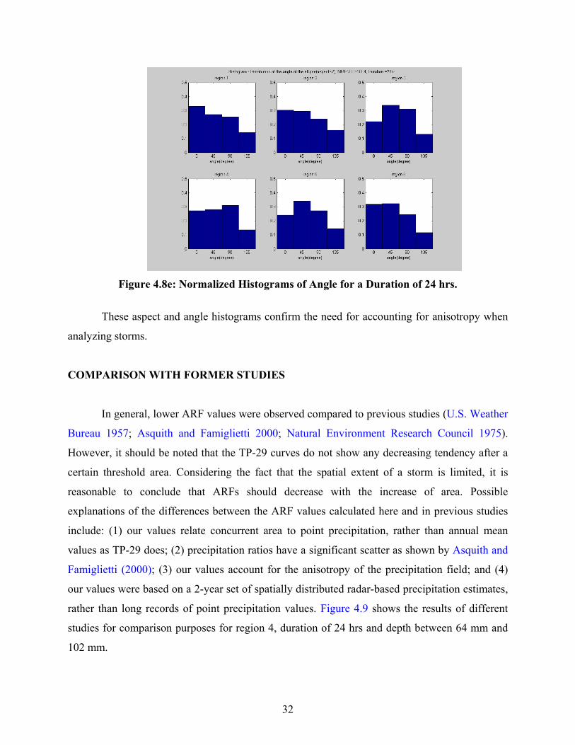
Similarly, normalized histograms of the orientation angle are presented in Figure 4.8 for

those ellipses with an aspect greater than 2. The aspect threshold of 2 was used because the angle

was considered a trivial variable for almost-circular ellipses. In these histograms, an angle of 0°

referred to an ellipse whose longer axis was parallel to the west-east direction, an angle of 45° to

an ellipse whose longer axis was parallel to the southwest-northeast direction, and so on. In the

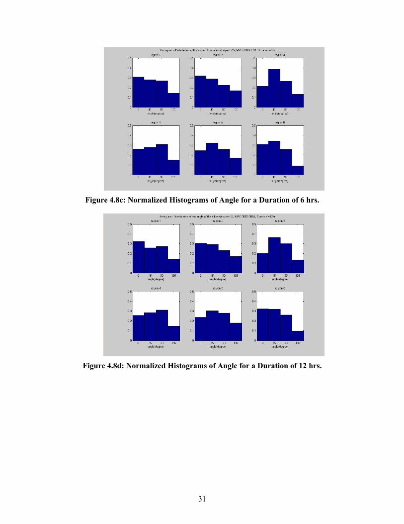
histograms, regional variability is significant. Overall, a clear predominance of a 45° angle was

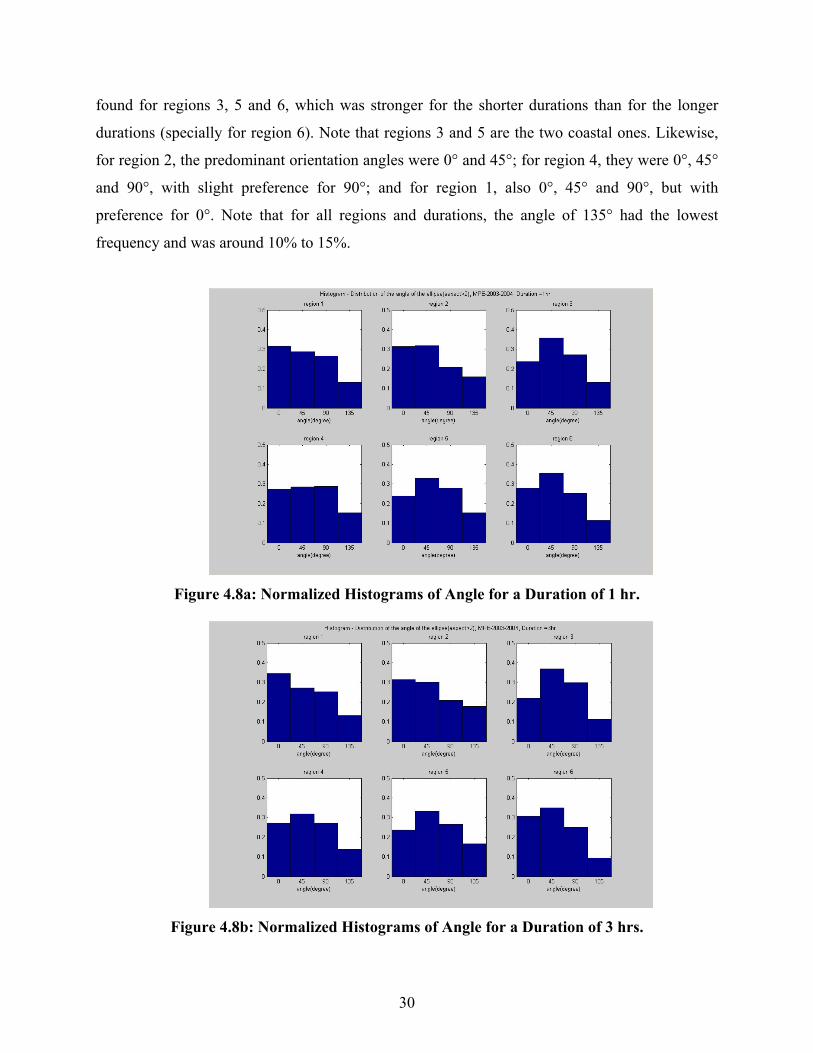
30

found for regions 3, 5 and 6, which was stronger for the shorter durations than for the longer

durations (specially for region 6). Note that regions 3 and 5 are the two coastal ones. Likewise,

for region 2, the predominant orientation angles were 0° and 45°; for region 4, they were 0°, 45°

and 90°, with slight preference for 90°; and for region 1, also 0°, 45° and 90°, but with

preference for 0°. Note that for all regions and durations, the angle of 135° had the lowest

frequency and was around 10% to 15%.

Figure 4.8a: Normalized Histograms of Angle for a Duration of 1 hr.

Figure 4.8b: Normalized Histograms of Angle for a Duration of 3 hrs.

31

Figure 4.8c: Normalized Histograms of Angle for a Duration of 6 hrs.

Figure 4.8d: Normalized Histograms of Angle for a Duration of 12 hrs.

32

Figure 4.8e: Normalized Histograms of Angle for a Duration of 24 hrs.

These aspect and angle histograms confirm the need for accounting for anisotropy when

analyzing storms.

COMPARISON WITH FORMER STUDIES

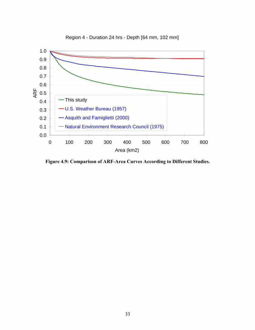
In general, lower ARF values were observed compared to previous studies (U.S. Weather

Bureau 1957; Asquith and Famiglietti 2000; Natural Environment Research Council 1975).

However, it should be noted that the TP-29 curves do not show any decreasing tendency after a

certain threshold area. Considering the fact that the spatial extent of a storm is limited, it is

reasonable to conclude that ARFs should decrease with the increase of area. Possible

explanations of the differences between the ARF values calculated here and in previous studies

include: (1) our values relate concurrent area to point precipitation, rather than annual mean

values as TP-29 does; (2) precipitation ratios have a significant scatter as shown by Asquith and

Famiglietti (2000); (3) our values account for the anisotropy of the precipitation field; and (4)

our values were based on a 2-year set of spatially distributed radar-based precipitation estimates,

rather than long records of point precipitation values. Figure 4.9 shows the results of different

studies for comparison purposes for region 4, duration of 24 hrs and depth between 64 mm and

102 mm.

33

Region 4 - Duration 24 hrs - Depth [64 mm, 102 mm]

0.0

0.1

0.2

0.3

0.4

0.5

0.6

0.7

0.8

0.9

1.0

0 100 200 300 400 500 600 700 800Area (km2)

AR

F

This study

U.S. Weather Bureau (1957)

Asquith and Famiglietti (2000)

Natural Environment Research Council (1975)

Figure 4.9: Comparison of ARF-Area Curves According to Different Studies.

35

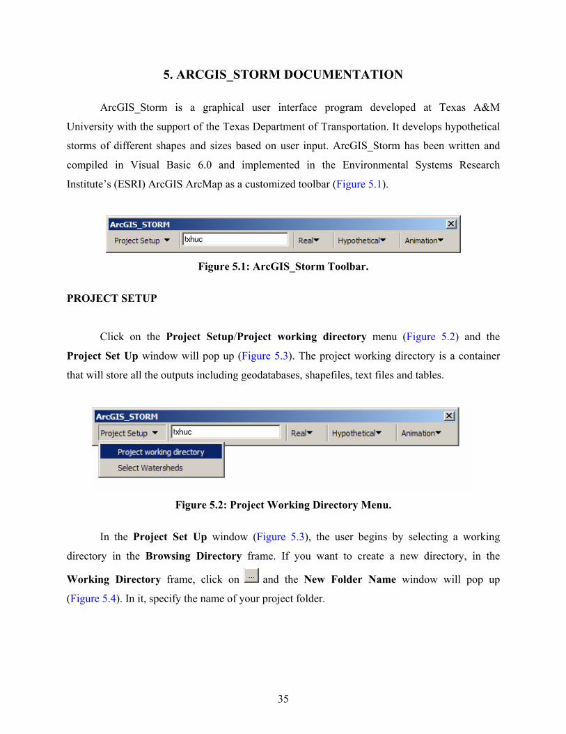
5. ARCGIS_STORM DOCUMENTATION

ArcGIS_Storm is a graphical user interface program developed at Texas A&M

University with the support of the Texas Department of Transportation. It develops hypothetical

storms of different shapes and sizes based on user input. ArcGIS_Storm has been written and

compiled in Visual Basic 6.0 and implemented in the Environmental Systems Research

Institute’s (ESRI) ArcGIS ArcMap as a customized toolbar (Figure 5.1).

Figure 5.1: ArcGIS_Storm Toolbar.

PROJECT SETUP

Click on the Project Setup/Project working directory menu (Figure 5.2) and the

Project Set Up window will pop up (Figure 5.3). The project working directory is a container

that will store all the outputs including geodatabases, shapefiles, text files and tables.

Figure 5.2: Project Working Directory Menu.

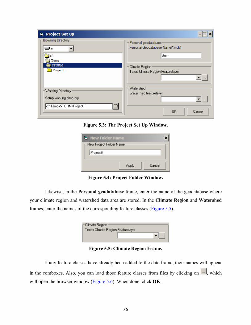
In the Project Set Up window (Figure 5.3), the user begins by selecting a working

directory in the Browsing Directory frame. If you want to create a new directory, in the

Working Directory frame, click on and the New Folder Name window will pop up

(Figure 5.4). In it, specify the name of your project folder.

36

Figure 5.3: The Project Set Up Window.

Figure 5.4: Project Folder Window.

Likewise, in the Personal geodatabase frame, enter the name of the geodatabase where

your climate region and watershed data area are stored. In the Climate Region and Watershed

frames, enter the names of the corresponding feature classes (Figure 5.5).

Figure 5.5: Climate Region Frame.

If any feature classes have already been added to the data frame, their names will appear

in the comboxes. Also, you can load those feature classes from files by clicking on , which

will open the browser window (Figure 5.6). When done, click OK.

37

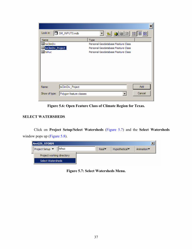
Figure 5.6: Open Feature Class of Climate Region for Texas.

SELECT WATERSHEDS

Click on Project Setup/Select Watersheds (Figure 5.7) and the Select Watersheds

window pops up (Figure 5.8).

Figure 5.7: Select Watersheds Menu.

38

Figure 5.8: Select Watersheds Window.

In Figure 5.8, the user begins by clicking on Select watershed polygon and selecting the

watershed polygons of interest on the map (Figure 5.9). The number of watersheds should be less

than 3. Once the watersheds are selected, click on Apply.

Figure 5.9: Example of Selecting Watersheds.

39

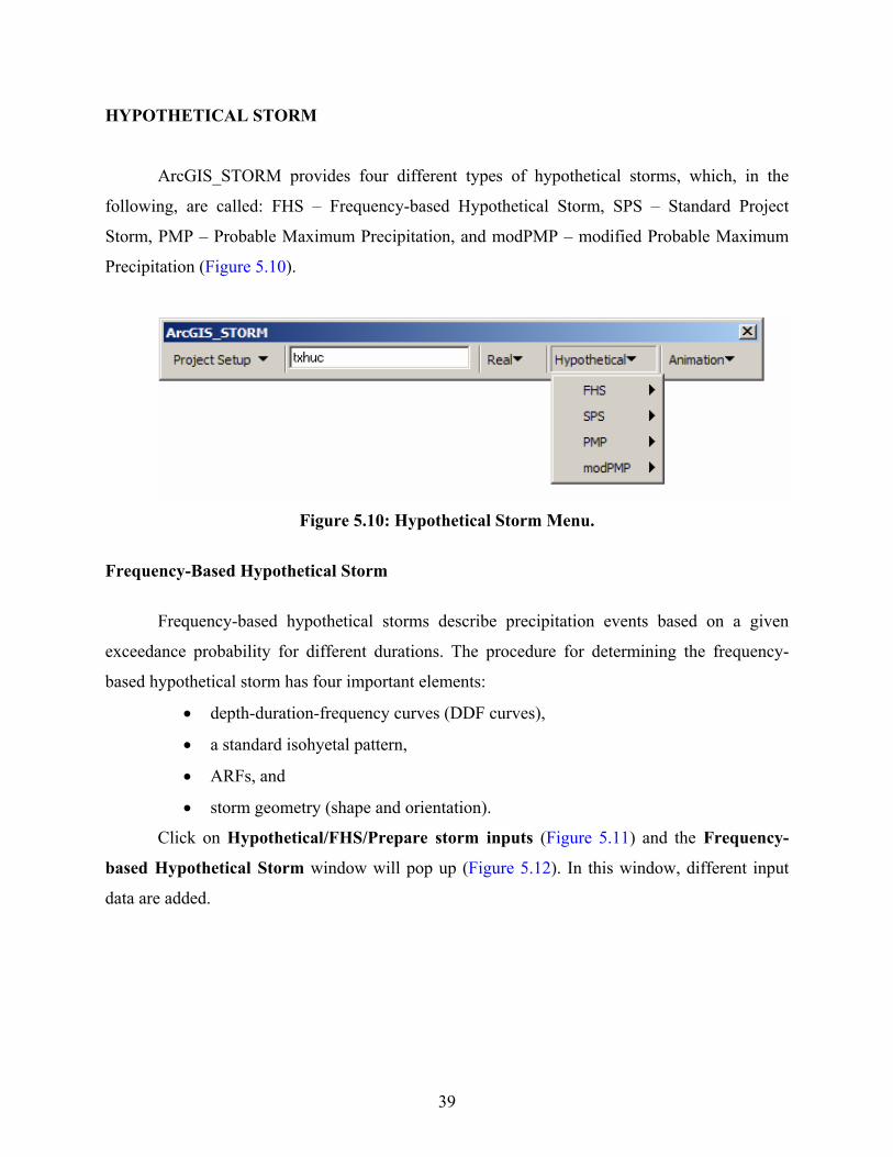
HYPOTHETICAL STORM

ArcGIS_STORM provides four different types of hypothetical storms, which, in the

following, are called: FHS – Frequency-based Hypothetical Storm, SPS – Standard Project

Storm, PMP – Probable Maximum Precipitation, and modPMP – modified Probable Maximum

Precipitation (Figure 5.10).

Figure 5.10: Hypothetical Storm Menu.

Frequency-Based Hypothetical Storm

Frequency-based hypothetical storms describe precipitation events based on a given

exceedance probability for different durations. The procedure for determining the frequency-

based hypothetical storm has four important elements:

• depth-duration-frequency curves (DDF curves),

• a standard isohyetal pattern,

• ARFs, and

• storm geometry (shape and orientation).

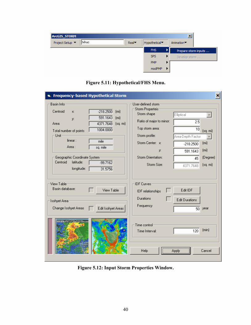
Click on Hypothetical/FHS/Prepare storm inputs (Figure 5.11) and the Frequency-

based Hypothetical Storm window will pop up (Figure 5.12). In this window, different input

data are added.

40

Figure 5.11: Hypothetical/FHS Menu.

Figure 5.12: Input Storm Properties Window.

41

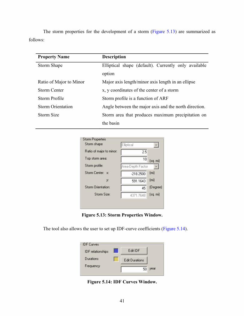
The storm properties for the development of a storm (Figure 5.13) are summarized as

follows:

Property Name Description

Storm Shape Elliptical shape (default). Currently only available

option

Ratio of Major to Minor Major axis length/minor axis length in an ellipse

Storm Center x, y coordinates of the center of a storm

Storm Profile Storm profile is a function of ARF

Storm Orientation Angle between the major axis and the north direction.

Storm Size Storm area that produces maximum precipitation on

the basin

Figure 5.13: Storm Properties Window.

The tool also allows the user to set up IDF-curve coefficients (Figure 5.14).

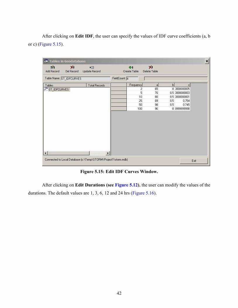
Figure 5.14: IDF Curves Window.

42

After clicking on Edit IDF, the user can specify the values of IDF curve coefficients (a, b

or c) (Figure 5.15).

Figure 5.15: Edit IDF Curves Window.

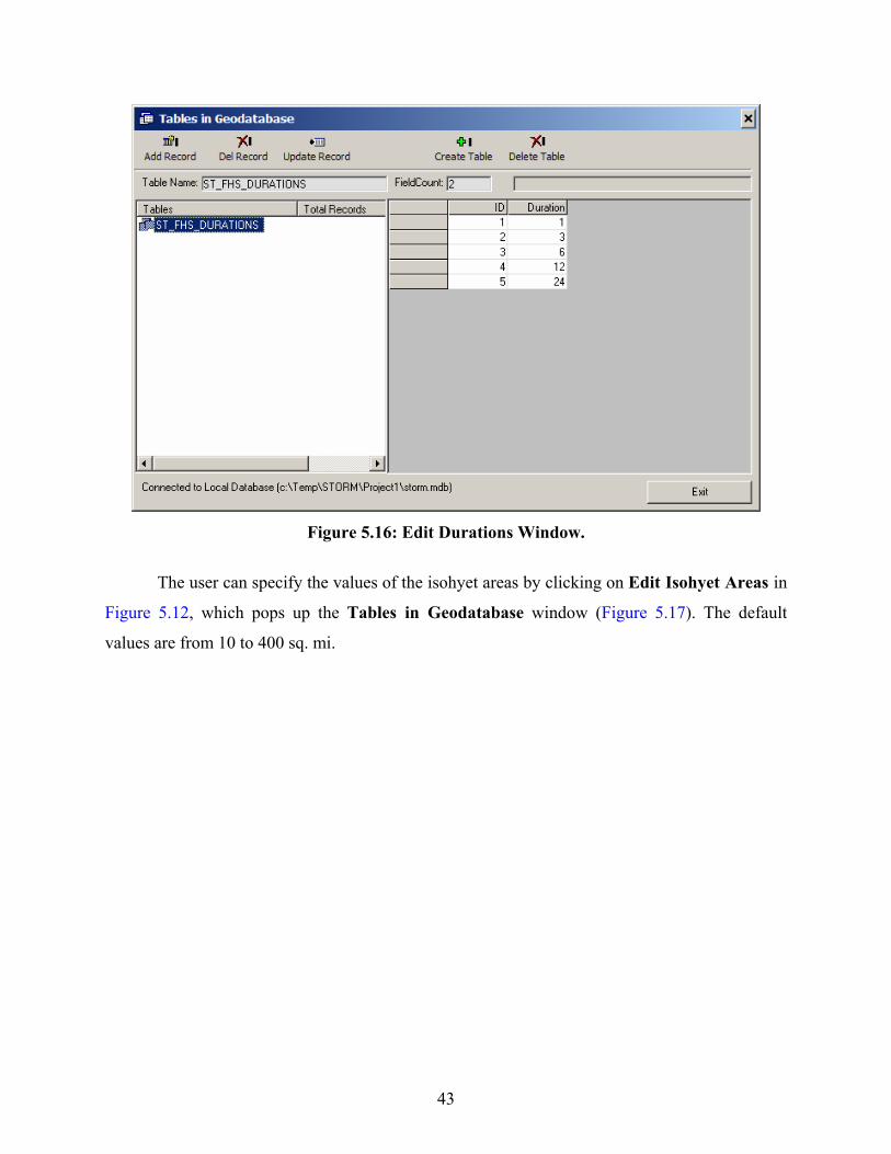
After clicking on Edit Durations (see Figure 5.12), the user can modify the values of the

durations. The default values are 1, 3, 6, 12 and 24 hrs (Figure 5.16).

43

Figure 5.16: Edit Durations Window.

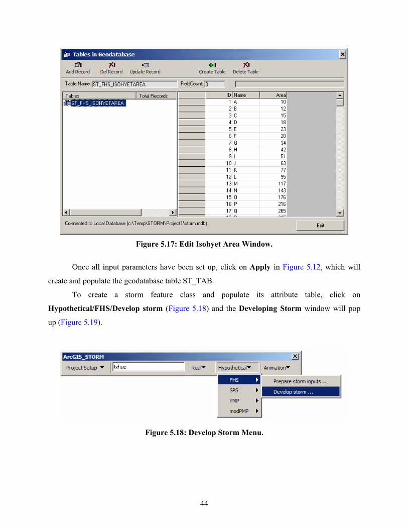
The user can specify the values of the isohyet areas by clicking on Edit Isohyet Areas in

Figure 5.12, which pops up the Tables in Geodatabase window (Figure 5.17). The default

values are from 10 to 400 sq. mi.

44

Figure 5.17: Edit Isohyet Area Window.

Once all input parameters have been set up, click on Apply in Figure 5.12, which will

create and populate the geodatabase table ST_TAB.

To create a storm feature class and populate its attribute table, click on

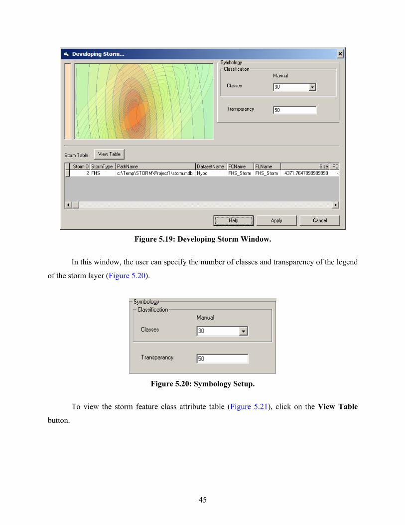
Hypothetical/FHS/Develop storm (Figure 5.18) and the Developing Storm window will pop

up (Figure 5.19).

Figure 5.18: Develop Storm Menu.

45

Figure 5.19: Developing Storm Window.

In this window, the user can specify the number of classes and transparency of the legend

of the storm layer (Figure 5.20).

Figure 5.20: Symbology Setup.

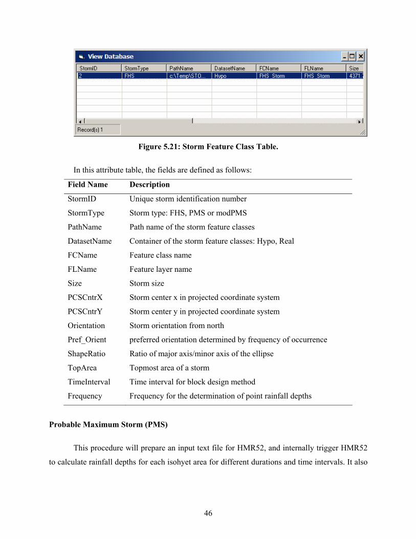
To view the storm feature class attribute table (Figure 5.21), click on the View Table

button.

46

Figure 5.21: Storm Feature Class Table.

In this attribute table, the fields are defined as follows:

Field Name Description

StormID Unique storm identification number

StormType Storm type: FHS, PMS or modPMS

PathName Path name of the storm feature classes

DatasetName Container of the storm feature classes: Hypo, Real

FCName Feature class name

FLName Feature layer name

Size Storm size

PCSCntrX Storm center x in projected coordinate system

PCSCntrY Storm center y in projected coordinate system

Orientation Storm orientation from north

Pref_Orient preferred orientation determined by frequency of occurrence

ShapeRatio Ratio of major axis/minor axis of the ellipse

TopArea Topmost area of a storm

TimeInterval Time interval for block design method

Frequency Frequency for the determination of point rainfall depths

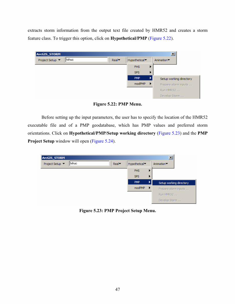
Probable Maximum Storm (PMS)

This procedure will prepare an input text file for HMR52, and internally trigger HMR52

to calculate rainfall depths for each isohyet area for different durations and time intervals. It also

47

extracts storm information from the output text file created by HMR52 and creates a storm

feature class. To trigger this option, click on Hypothetical/PMP (Figure 5.22).

Figure 5.22: PMP Menu.

Before setting up the input parameters, the user has to specify the location of the HMR52

executable file and of a PMP geodatabase, which has PMP values and preferred storm

orientations. Click on Hypothetical/PMP/Setup working directory (Figure 5.23) and the PMP

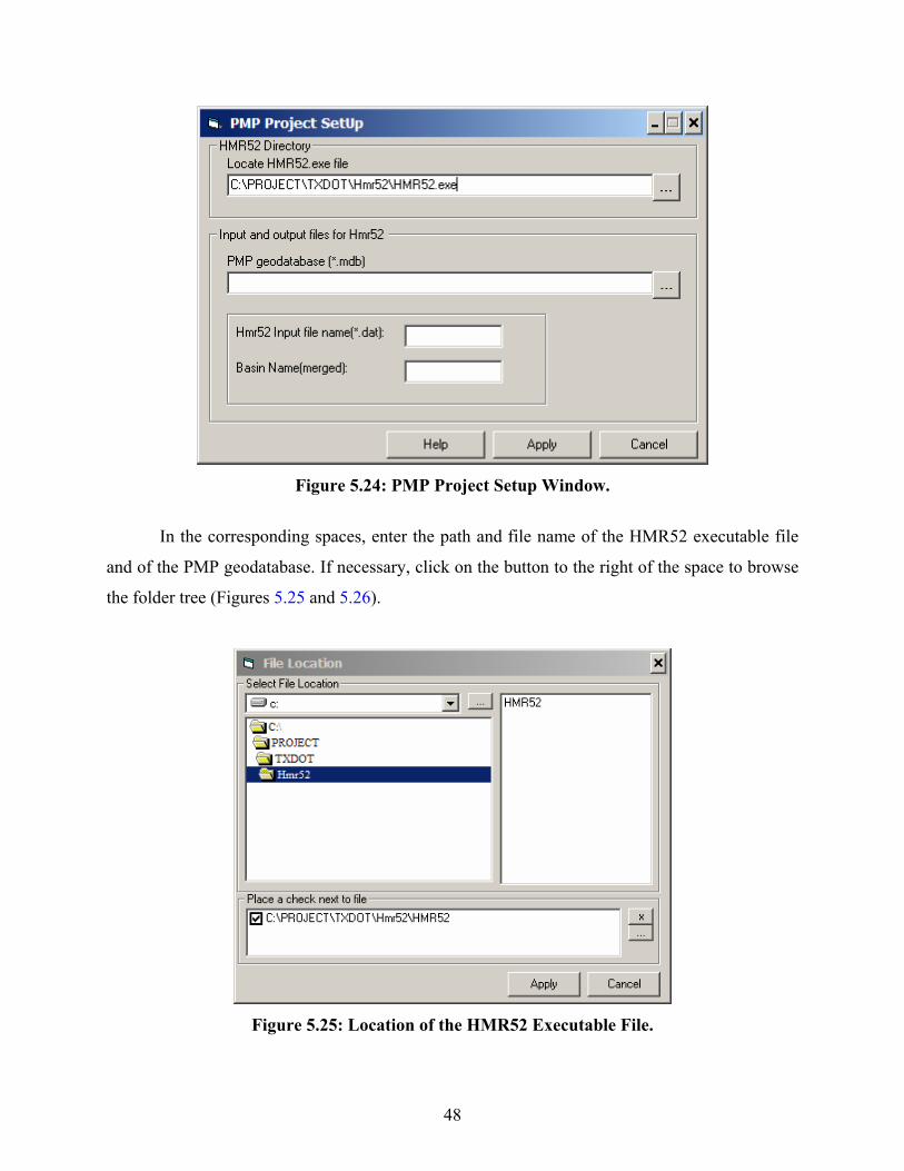
Project Setup window will open (Figure 5.24).

Figure 5.23: PMP Project Setup Menu.

48

Figure 5.24: PMP Project Setup Window.

In the corresponding spaces, enter the path and file name of the HMR52 executable file

and of the PMP geodatabase. If necessary, click on the button to the right of the space to browse

the folder tree (Figures 5.25 and 5.26).

Figure 5.25: Location of the HMR52 Executable File.

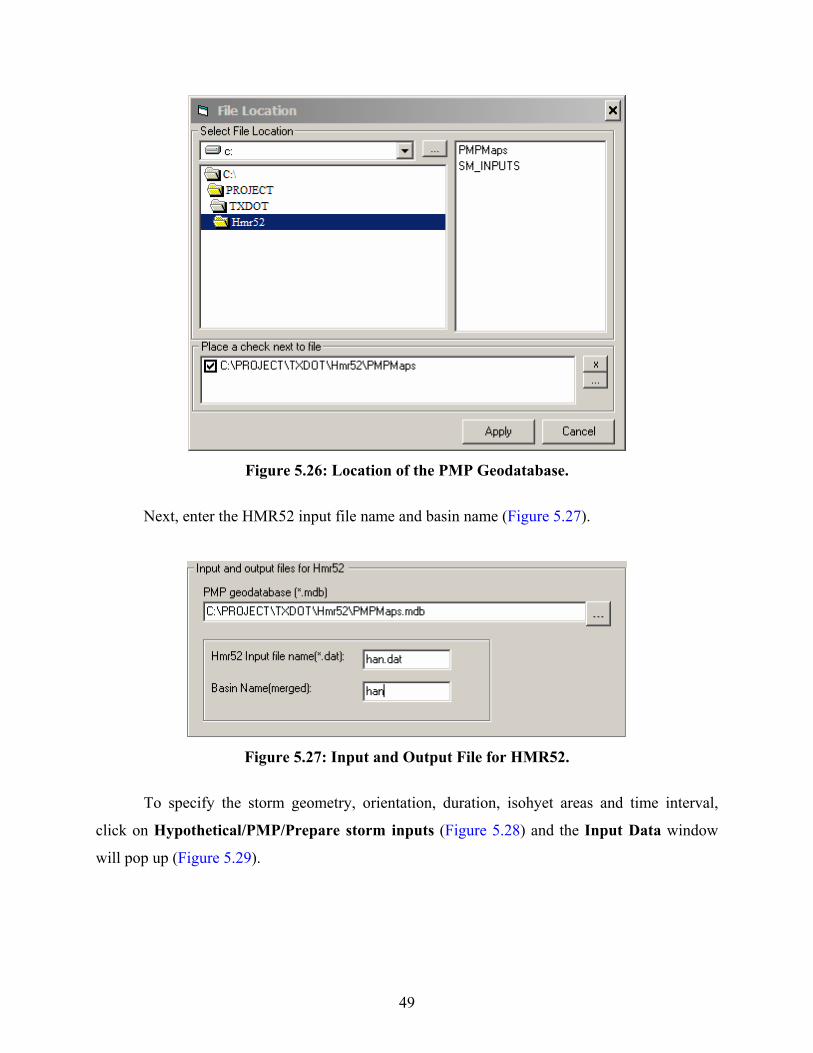
49

Figure 5.26: Location of the PMP Geodatabase.

Next, enter the HMR52 input file name and basin name (Figure 5.27).

Figure 5.27: Input and Output File for HMR52.

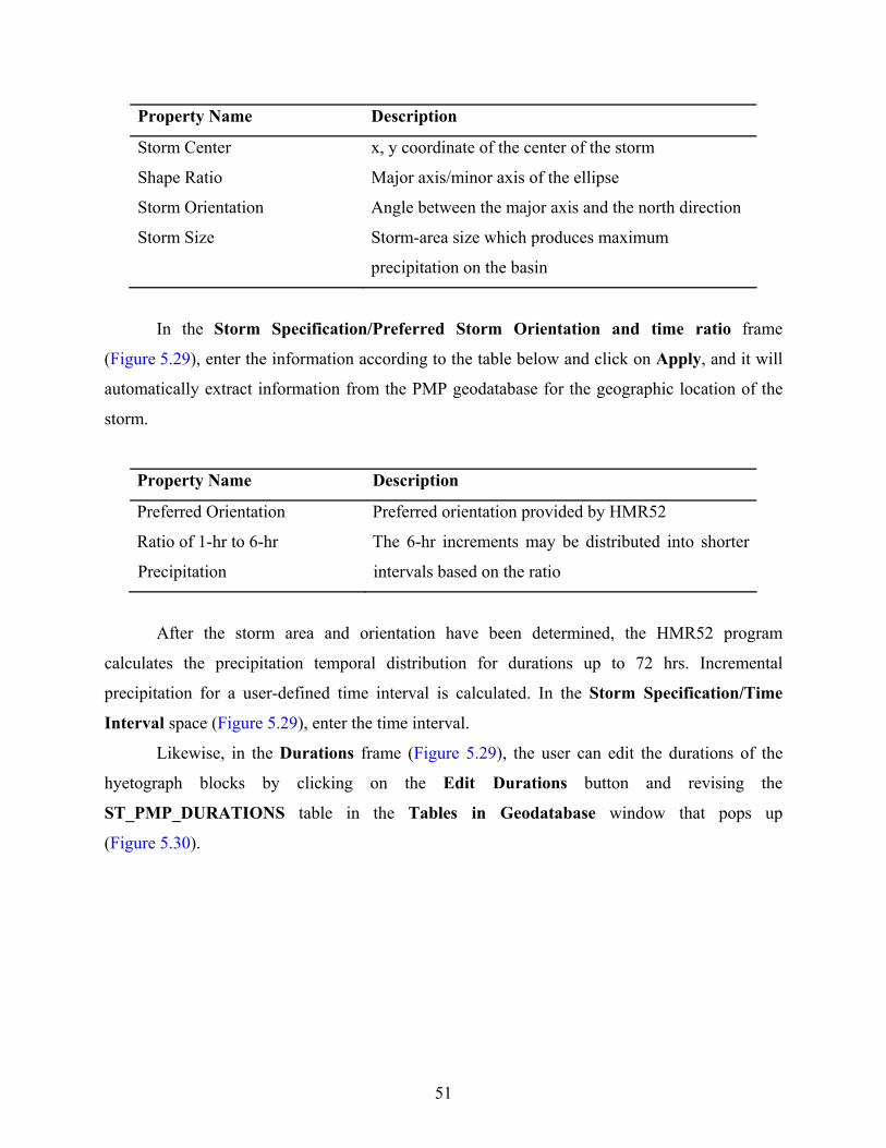
To specify the storm geometry, orientation, duration, isohyet areas and time interval,

click on Hypothetical/PMP/Prepare storm inputs (Figure 5.28) and the Input Data window

will pop up (Figure 5.29).

50

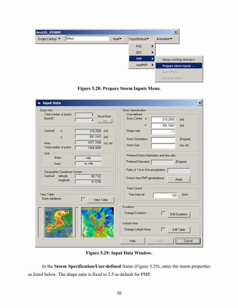
Figure 5.28: Prepare Storm Inputs Menu.

Figure 5.29: Input Data Window.

In the Storm Specification/User-defined frame (Figure 5.29), enter the storm properties

as listed below. The shape ratio is fixed to 2.5 as default for PMP.

51


Storm Center x, y coordinate of the center of the storm

Shape Ratio Major axis/minor axis of the ellipse

Storm Orientation Angle between the major axis and the north direction

Storm Size Storm-area size which produces maximum

precipitation on the basin

In the Storm Specification/Preferred Storm Orientation and time ratio frame

(Figure 5.29), enter the information according to the table below and click on Apply, and it will

automatically extract information from the PMP geodatabase for the geographic location of the

storm.


Preferred Orientation Preferred orientation provided by HMR52

Ratio of 1-hr to 6-hr

Precipitation

The 6-hr increments may be distributed into shorter

intervals based on the ratio

After the storm area and orientation have been determined, the HMR52 program

calculates the precipitation temporal distribution for durations up to 72 hrs. Incremental

precipitation for a user-defined time interval is calculated. In the Storm Specification/Time

Interval space (Figure 5.29), enter the time interval.

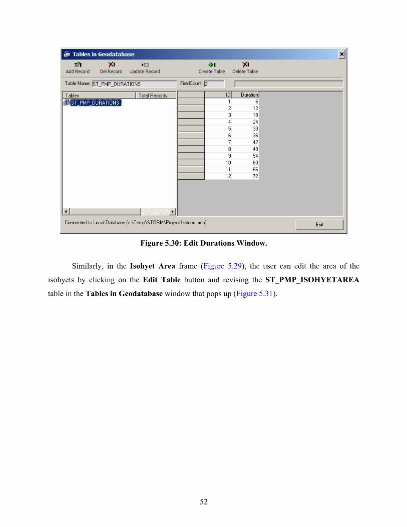
Likewise, in the Durations frame (Figure 5.29), the user can edit the durations of the

hyetograph blocks by clicking on the Edit Durations button and revising the

ST_PMP_DURATIONS table in the Tables in Geodatabase window that pops up

(Figure 5.30).

52

Figure 5.30: Edit Durations Window.

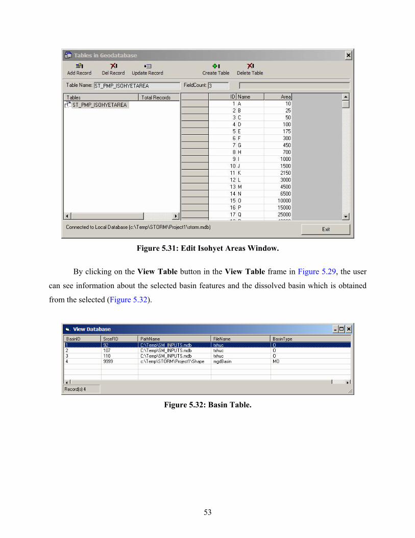
Similarly, in the Isohyet Area frame (Figure 5.29), the user can edit the area of the

isohyets by clicking on the Edit Table button and revising the ST_PMP_ISOHYETAREA

table in the Tables in Geodatabase window that pops up (Figure 5.31).

53

Figure 5.31: Edit Isohyet Areas Window.

By clicking on the View Table button in the View Table frame in Figure 5.29, the user

can see information about the selected basin features and the dissolved basin which is obtained

from the selected (Figure 5.32).

Figure 5.32: Basin Table.

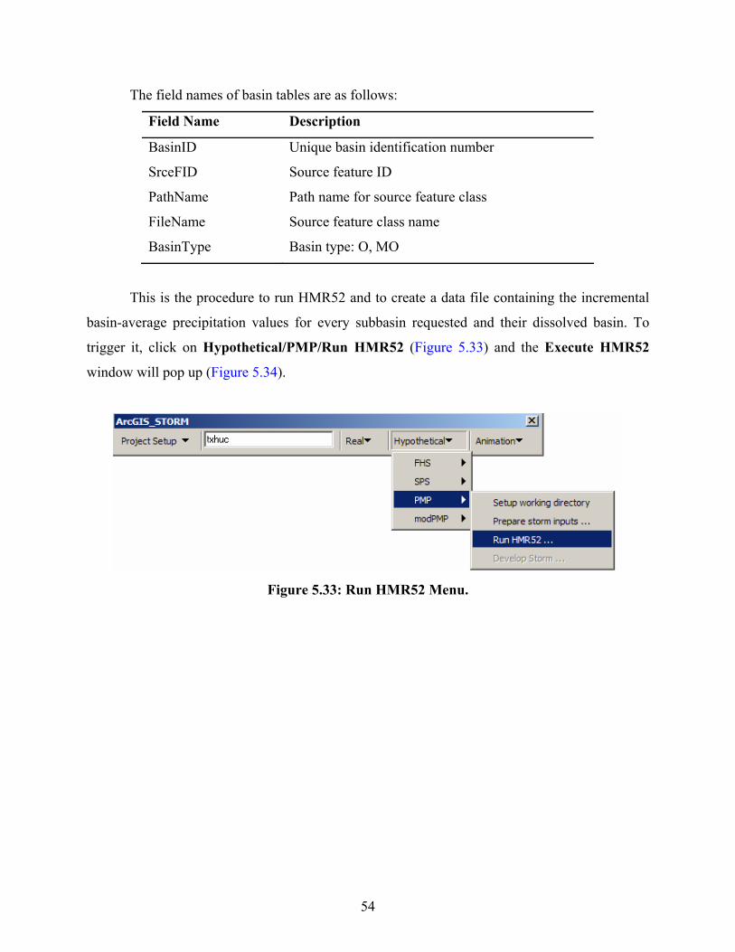
54

The field names of basin tables are as follows:

Field Name Description

BasinID Unique basin identification number

SrceFID Source feature ID

PathName Path name for source feature class

FileName Source feature class name

BasinType Basin type: O, MO

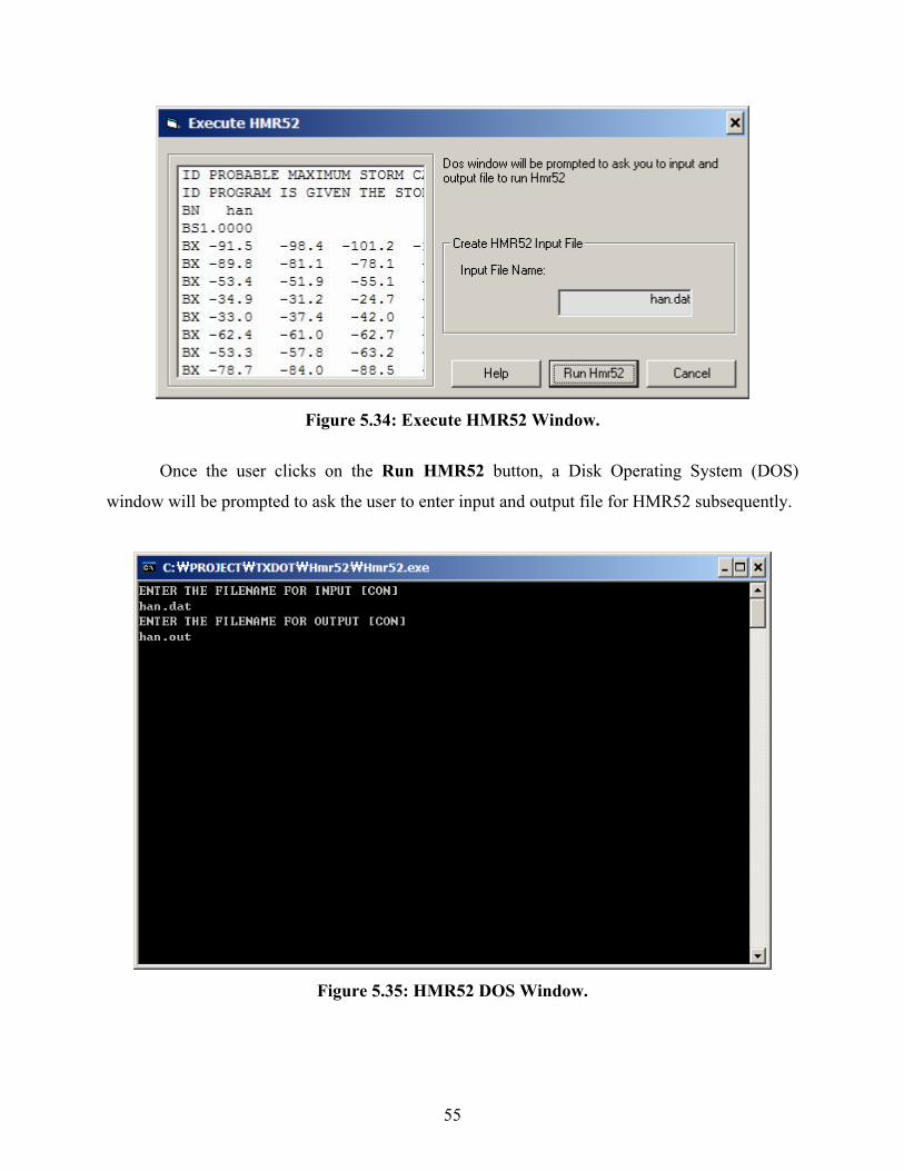
This is the procedure to run HMR52 and to create a data file containing the incremental

basin-average precipitation values for every subbasin requested and their dissolved basin. To

trigger it, click on Hypothetical/PMP/Run HMR52 (Figure 5.33) and the Execute HMR52

window will pop up (Figure 5.34).

Figure 5.33: Run HMR52 Menu.

55

Figure 5.34: Execute HMR52 Window.

Once the user clicks on the Run HMR52 button, a Disk Operating System (DOS)

window will be prompted to ask the user to enter input and output file for HMR52 subsequently.

Figure 5.35: HMR52 DOS Window.

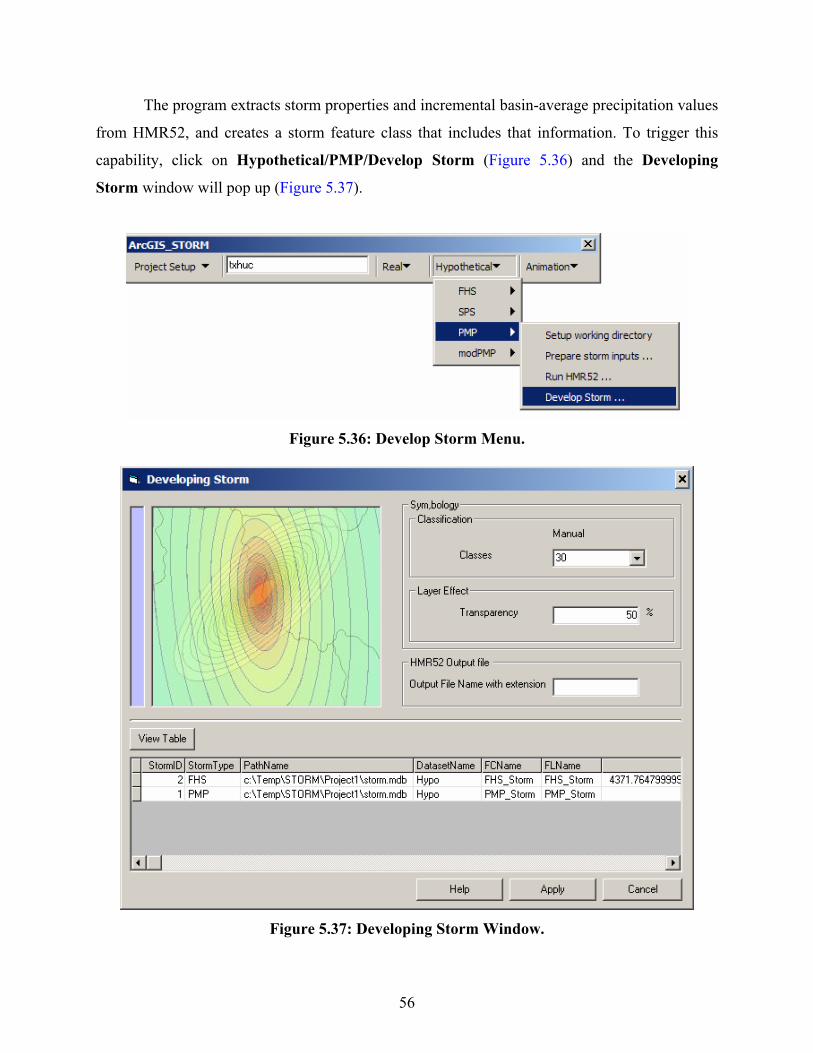
56

The program extracts storm properties and incremental basin-average precipitation values

from HMR52, and creates a storm feature class that includes that information. To trigger this

capability, click on Hypothetical/PMP/Develop Storm (Figure 5.36) and the Developing

Storm window will pop up (Figure 5.37).

Figure 5.36: Develop Storm Menu.

Figure 5.37: Developing Storm Window.

57

In the Symbology frame (Figure 5.37), the user can specify the number of classes and

transparency of the storm feature layer. In the HMR52 Output file frame (Figure 5.37), the user

also has to enter the name of the HMR52 output file. The program will use storm information

from this data file to create a storm feature class.

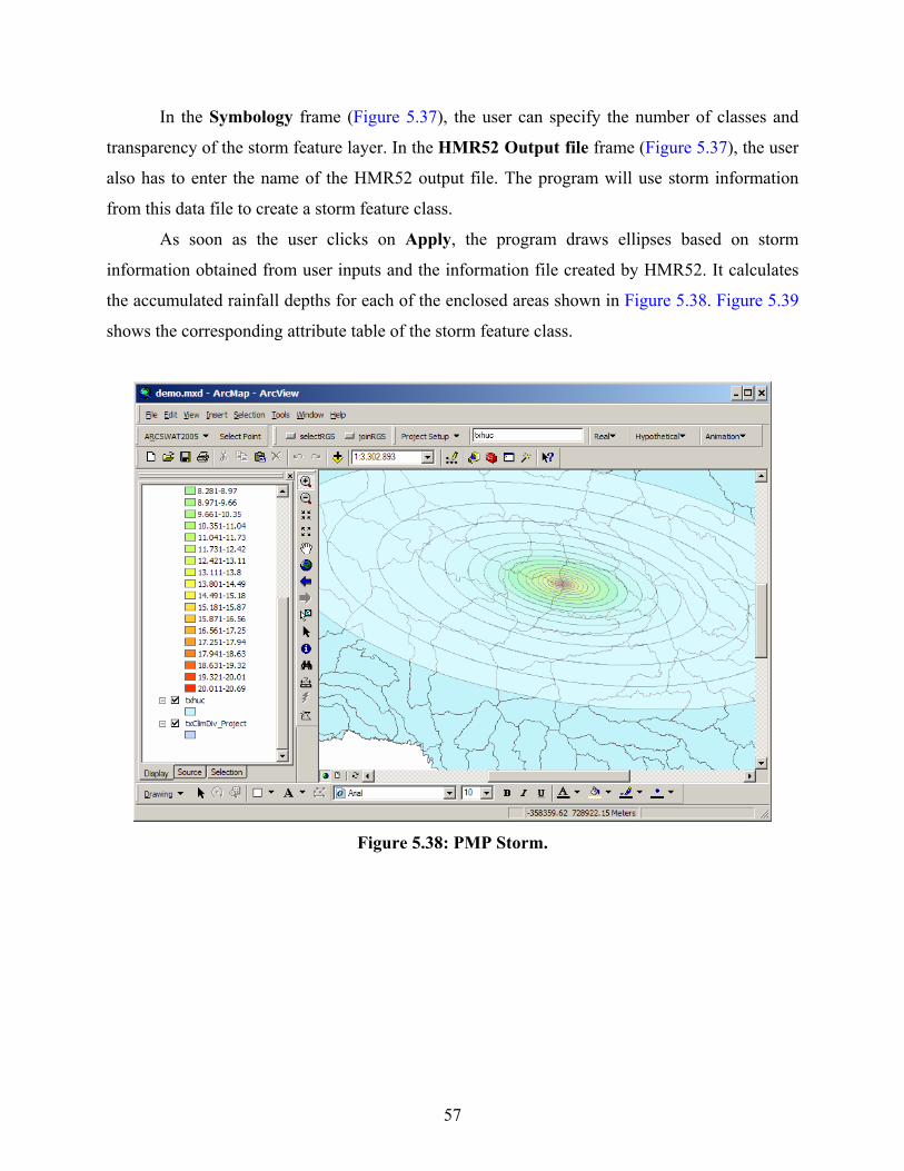
As soon as the user clicks on Apply, the program draws ellipses based on storm

information obtained from user inputs and the information file created by HMR52. It calculates

the accumulated rainfall depths for each of the enclosed areas shown in Figure 5.38. Figure 5.39

shows the corresponding attribute table of the storm feature class.

Figure 5.38: PMP Storm.

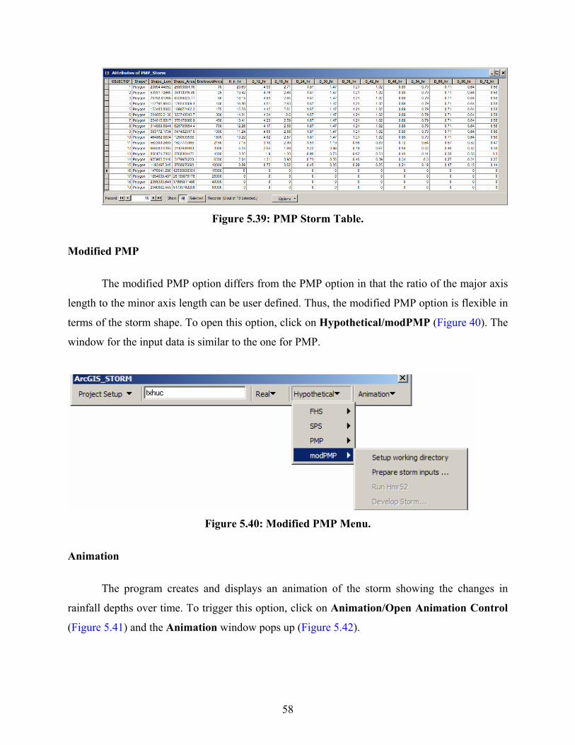
58

Figure 5.39: PMP Storm Table.

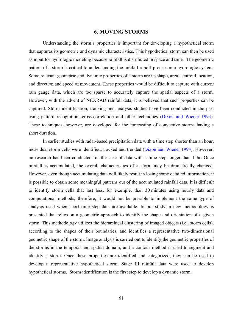
Modified PMP

The modified PMP option differs from the PMP option in that the ratio of the major axis

length to the minor axis length can be user defined. Thus, the modified PMP option is flexible in

terms of the storm shape. To open this option, click on Hypothetical/modPMP (Figure 40). The

window for the input data is similar to the one for PMP.

Figure 5.40: Modified PMP Menu.

Animation

The program creates and displays an animation of the storm showing the changes in

rainfall depths over time. To trigger this option, click on Animation/Open Animation Control

(Figure 5.41) and the Animation window pops up (Figure 5.42).

59

Figure 5.41: Animation Toolbar.

Figure 5.42: Animation Setup Window.

61

6. MOVING STORMS

Understanding the storm’s properties is important for developing a hypothetical storm

that captures its geometric and dynamic characteristics. This hypothetical storm can then be used

as input for hydrologic modeling because rainfall is distributed in space and time. The geometric

pattern of a storm is critical to understanding the rainfall-runoff process in a hydrologic system.

Some relevant geometric and dynamic properties of a storm are its shape, area, centroid location,

and direction and speed of movement. These properties would be difficult to capture with current

rain gauge data, which are too sparse to accurately capture the spatial aspects of a storm.

However, with the advent of NEXRAD rainfall data, it is believed that such properties can be

captured. Storm identification, tracking and analysis studies have been conducted in the past

using pattern recognition, cross-correlation and other techniques (Dixon and Wiener 1993).

These techniques, however, are developed for the forecasting of convective storms having a

short duration.

In earlier studies with radar-based precipitation data with a time step shorter than an hour,

individual storm cells were identified, tracked and trended (Dixon and Wiener 1993). However,

no research has been conducted for the case of data with a time step longer than 1 hr. Once

rainfall is accumulated, the overall characteristics of a storm may be dramatically changed.

However, even though accumulating data will likely result in losing some detailed information, it

is possible to obtain some meaningful patterns out of the accumulated rainfall data. It is difficult

to identify storm cells that last less, for example, than 30 minutes using hourly data and

computational methods; therefore, it would not be possible to implement the same type of

analysis used when short time step data are available. In our study, a new methodology is

presented that relies on a geometric approach to identify the shape and orientation of a given

storm. This methodology utilizes the hierarchical clustering of imaged objects (i.e., storm cells),

according to the shapes of their boundaries, and identifies a representative two-dimensional

geometric shape of the storm. Image analysis is carried out to identify the geometric properties of

the storms in the temporal and spatial domain, and a contour method is used to segment and

identify a storm. Once these properties are identified and categorized, they can be used to

develop a representative hypothetical storm. Stage III rainfall data were used to develop

hypothetical storms. Storm identification is the first step to develop a dynamic storm.

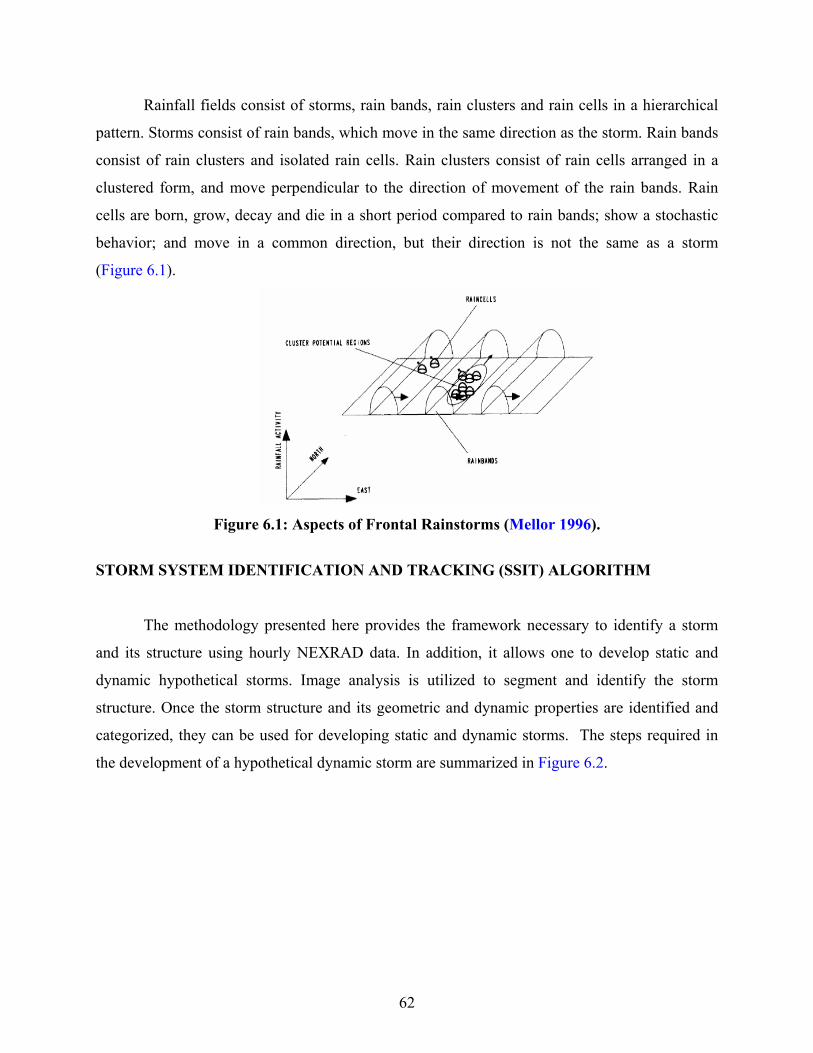
62

Rainfall fields consist of storms, rain bands, rain clusters and rain cells in a hierarchical

pattern. Storms consist of rain bands, which move in the same direction as the storm. Rain bands

consist of rain clusters and isolated rain cells. Rain clusters consist of rain cells arranged in a

clustered form, and move perpendicular to the direction of movement of the rain bands. Rain

cells are born, grow, decay and die in a short period compared to rain bands; show a stochastic

behavior; and move in a common direction, but their direction is not the same as a storm

(Figure 6.1).

Figure 6.1: Aspects of Frontal Rainstorms (Mellor 1996).

STORM SYSTEM IDENTIFICATION AND TRACKING (SSIT) ALGORITHM

The methodology presented here provides the framework necessary to identify a storm

and its structure using hourly NEXRAD data. In addition, it allows one to develop static and

dynamic hypothetical storms. Image analysis is utilized to segment and identify the storm

structure. Once the storm structure and its geometric and dynamic properties are identified and

categorized, they can be used for developing static and dynamic storms. The steps required in

the development of a hypothetical dynamic storm are summarized in Figure 6.2.

63

Spatial Analysis

Statistical Pattern Analysis

Geostatistical Analysis

Design Storm

Static design storm

Dynamic design storm

Spatial correlation: Moving storm analysisConvolution: Impact of moving storm

Feature extraction: Linear Discriminant Analysis, Principal Component Analysis (PCA), Kernel PCAProbability distribution estimation and clustering: Gaussian mixture model, K-means clustering

Trend analysis - mapping a trend: interpolating ARF, Storm properties (orientation, velocity) etc.

Figure 6.2: Storm Analysis.

Data Preparation

The SSIT algorithm was used to process the Stage III rainfall data of the West Gulf River

Forecast Center. Rainfall depths in the HRAP grid system were the only information contained

in the dataset. The cells of the annual maximum rainfall are identified and saved as a database

file. The storms that enclose the cells of annual maximum rainfall depths are the only cells

considered in this study.

Storm Detection Method

The general procedure is that the algorithm detects the boundaries of a storm, labels an

identified storm object in a pre-defined window and calculates statistical properties of each

identified storm object.

Segmentation

Three different image-processing methods are utilized to segment and identify storm

bands, storm clusters and storm cells, which are the Sobel method, the Canny algorithm and the

contour method. The Sobel and Canny algorithms use black and white images, referred to as

binary images, to segment an object. The image is converted to binary format to determine the

storm structure and area using feature detection methods. The contour method, on the other hand,

is based on rainfall values.

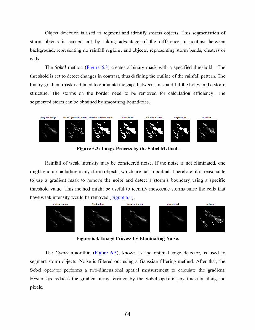
64

Object detection is used to segment and identify storms objects. This segmentation of

storm objects is carried out by taking advantage of the difference in contrast between

background, representing no rainfall regions, and objects, representing storm bands, clusters or

cells.

The Sobel method (Figure 6.3) creates a binary mask with a specified threshold. The

threshold is set to detect changes in contrast, thus defining the outline of the rainfall pattern. The

binary gradient mask is dilated to eliminate the gaps between lines and fill the holes in the storm

structure. The storms on the border need to be removed for calculation efficiency. The

segmented storm can be obtained by smoothing boundaries.

Figure 6.3: Image Process by the Sobel Method.

Rainfall of weak intensity may be considered noise. If the noise is not eliminated, one

might end up including many storm objects, which are not important. Therefore, it is reasonable

to use a gradient mask to remove the noise and detect a storm’s boundary using a specific

threshold value. This method might be useful to identify mesoscale storms since the cells that

have weak intensity would be removed (Figure 6.4).

Figure 6.4: Image Process by Eliminating Noise.

The Canny algorithm (Figure 6.5), known as the optimal edge detector, is used to

segment storm objects. Noise is filtered out using a Gaussian filtering method. After that, the

Sobel operator performs a two-dimensional spatial measurement to calculate the gradient.

Hysteresys reduces the gradient array, created by the Sobel operator, by tracking along the

pixels.

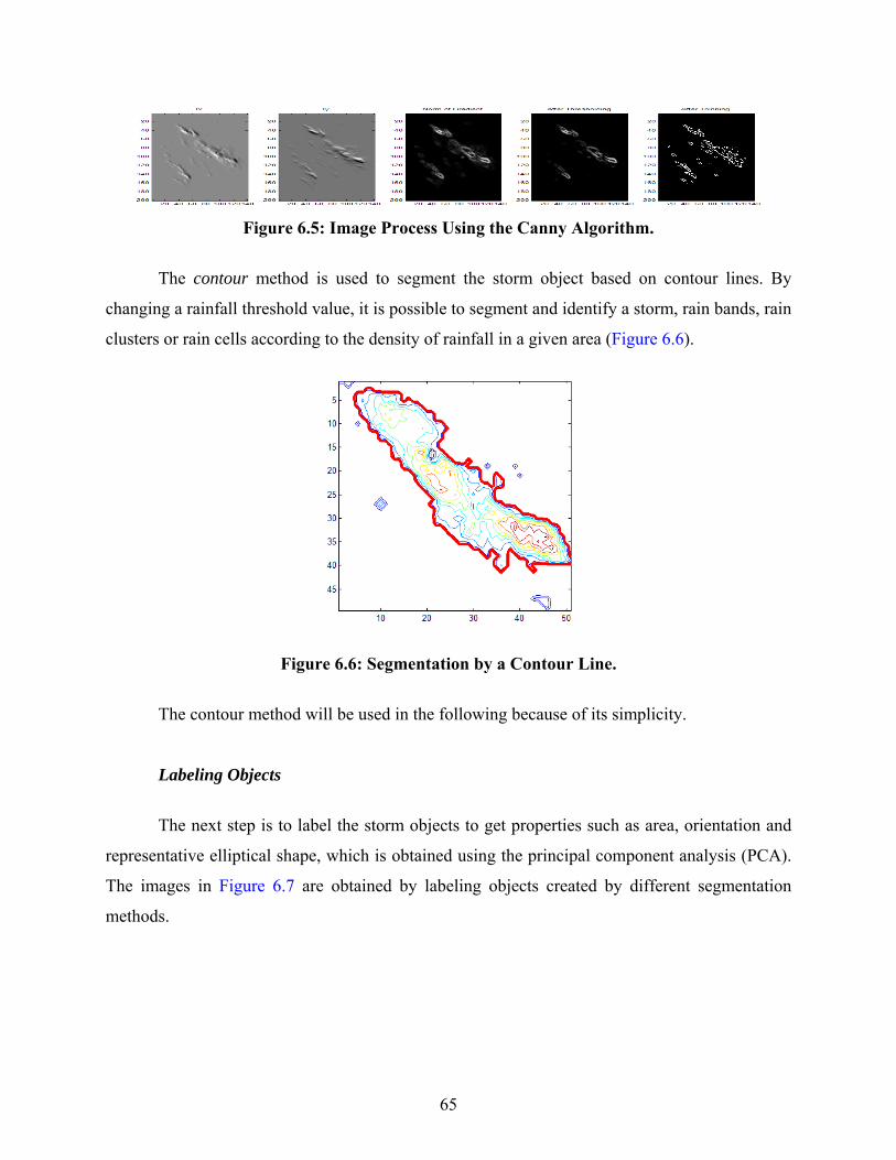
65

Figure 6.5: Image Process Using the Canny Algorithm.

The contour method is used to segment the storm object based on contour lines. By

changing a rainfall threshold value, it is possible to segment and identify a storm, rain bands, rain

clusters or rain cells according to the density of rainfall in a given area (Figure 6.6).

Figure 6.6: Segmentation by a Contour Line.

The contour method will be used in the following because of its simplicity.

Labeling Objects

The next step is to label the storm objects to get properties such as area, orientation and

representative elliptical shape, which is obtained using the principal component analysis (PCA).

The images in Figure 6.7 are obtained by labeling objects created by different segmentation

methods.

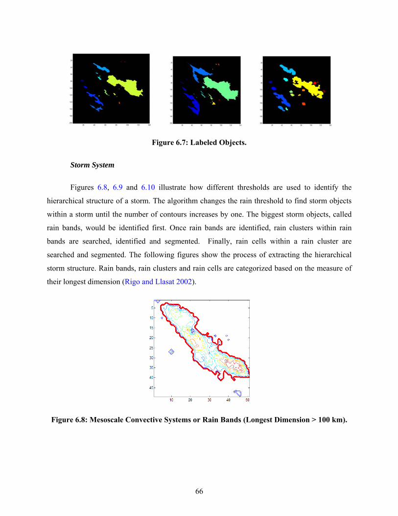
66

Figure 6.7: Labeled Objects.

Storm System

Figures 6.8, 6.9 and 6.10 illustrate how different thresholds are used to identify the

hierarchical structure of a storm. The algorithm changes the rain threshold to find storm objects

within a storm until the number of contours increases by one. The biggest storm objects, called

rain bands, would be identified first. Once rain bands are identified, rain clusters within rain

bands are searched, identified and segmented. Finally, rain cells within a rain cluster are

searched and segmented. The following figures show the process of extracting the hierarchical

storm structure. Rain bands, rain clusters and rain cells are categorized based on the measure of

their longest dimension (Rigo and Llasat 2002).

Figure 6.8: Mesoscale Convective Systems or Rain Bands (Longest Dimension > 100 km).

67

Figure 6.9: Multicell Storms or Rain Cluster (Longest Dimension < 100 km).

Figure 6.10: Rain Cells (Longest Dimension ≈ 5 km).

Storm Tracking

Once a storm is identified, its geometric properties are calculated. The geometric

properties can be centroid location, orientation and ratio of major axis length to minor axis length

when a storm is represented as an ellipse. The storm can then be matched in terms of similarity

of properties to other past storms. A function, representing a degree of similarity, would be used

to locate the storm at a later time, and determine the direction and speed of motion.

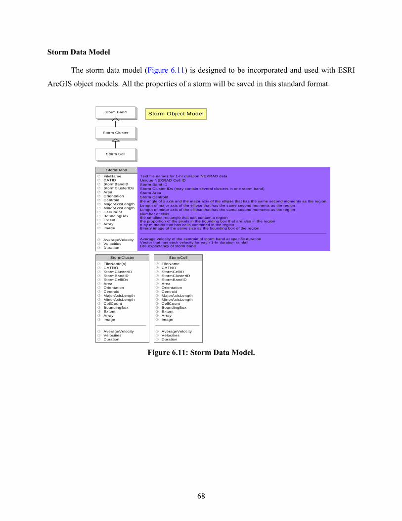
68

Storm Data Model

The storm data model (Figure 6.11) is designed to be incorporated and used with ESRI

ArcGIS object models. All the properties of a storm will be saved in this standard format.

Storm Band

Storm Cluster

Storm Cell

StormBand

FileNameCATIDStormBandIDStormClusterIDsAreaOrientationCentroidMajorAxisLengthMinorAxisLengthCellCountBoundingBoxExtentArrayImage

________________

AverageVelocityVelocitiesDuration

StormCell

FileNameCATNOStormCellIDStormClusterIDStormBandIDAreaOrientationCentroidMajorAxisLengthMinorAxisLengthCellCountBoundingBoxExtentArrayImage

___________________


StormCluster

FileName(s)CATNOStormClusterIDStormBandIDStormCellIDsAreaOrientationCentroidMajorAxisLengthMinorAxisLengthCellCountBoundingBoxExtentArrayImage

_____________________


Text file names for 1-hr duration NEXRAD dataUnique NEXRAD Cell IDStorm Band IDStorm Cluster IDs (may contain several clusters in one storm band)Storm AreaStorm Centroidthe angle of x axis and the major axis of the ellipse that has the same second moments as the regionLength of major axis of the ellipse that has the same second moments as the regionLength of minor axis of the ellipse that has the same second moments as the regionNumber of cells the smallest rectangle that can contain a regionthe proportion of the pixels in the bounding box that are also in the regionn by m matrix that has cells contained in the regionBinary image of the same size as the bounding box of the region________________________________________________________________________________

Average velocity of the centroid of storm band at specific durationVector that has each velocity for each 1-hr duration rainfallLife expectancy of storm band

Storm Object Model

Figure 6.11: Storm Data Model.

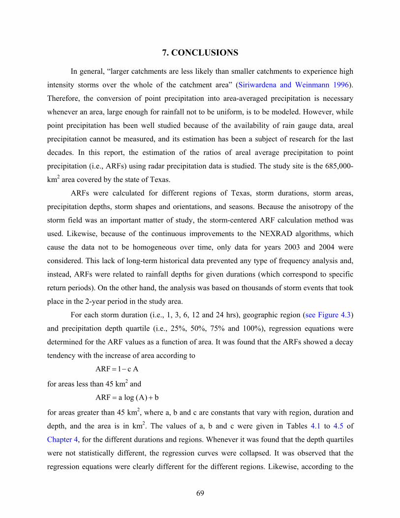
69

7. CONCLUSIONS

In general, “larger catchments are less likely than smaller catchments to experience high

intensity storms over the whole of the catchment area” (Siriwardena and Weinmann 1996).

Therefore, the conversion of point precipitation into area-averaged precipitation is necessary

whenever an area, large enough for rainfall not to be uniform, is to be modeled. However, while

point precipitation has been well studied because of the availability of rain gauge data, areal

precipitation cannot be measured, and its estimation has been a subject of research for the last

decades. In this report, the estimation of the ratios of areal average precipitation to point

precipitation (i.e., ARFs) using radar precipitation data is studied. The study site is the 685,000-

km2 area covered by the state of Texas.

ARFs were calculated for different regions of Texas, storm durations, storm areas,

precipitation depths, storm shapes and orientations, and seasons. Because the anisotropy of the

storm field was an important matter of study, the storm-centered ARF calculation method was

used. Likewise, because of the continuous improvements to the NEXRAD algorithms, which

cause the data not to be homogeneous over time, only data for years 2003 and 2004 were

considered. This lack of long-term historical data prevented any type of frequency analysis and,

instead, ARFs were related to rainfall depths for given durations (which correspond to specific

return periods). On the other hand, the analysis was based on thousands of storm events that took

place in the 2-year period in the study area.

For each storm duration (i.e., 1, 3, 6, 12 and 24 hrs), geographic region (see Figure 4.3)

and precipitation depth quartile (i.e., 25%, 50%, 75% and 100%), regression equations were

determined for the ARF values as a function of area. It was found that the ARFs showed a decay

tendency with the increase of area according to

ARF 1 c A= −

for areas less than 45 km2 and

ARF a log (A) b= +

for areas greater than 45 km2, where a, b and c are constants that vary with region, duration and

depth, and the area is in km2. The values of a, b and c were given in Tables 4.1 to 4.5 of

Chapter 4, for the different durations and regions. Whenever it was found that the depth quartiles

were not statistically different, the regression curves were collapsed. It was observed that the

regression equations were clearly different for the different regions. Likewise, according to the

70

depth-duration-frequency curve concept, depth and frequency are related for a given duration.

So, since it was observed that the ARFs increased with depth, it was concluded that they also

increase with return period.

Histograms of the aspect of the ellipses that represented the storms suggest that around

one-third of the ellipses had an aspect between 1 and 2, which corresponds to almost-circular

shapes. The remaining two-thirds of the storms had a clear elliptical shape with an aspect greater

than 2. It was also observed that the frequency decreased as the aspect increased. Overall the

same patterns were observed for the different regions and durations. Likewise, histograms of the

orientation angle show a clear predominance of a 45° angle for regions 3, 5 and 6, which was

stronger for the shorter durations than for the longer durations (specially for region 6). Note that

regions 3 and 5 are the two coastal ones. Additionally, for region 2, the predominant orientation

angles were 0° and 45°; for region 4, there was a slight preference for 90°; and for region 1, a

slight preference for 0°. Note that for all regions and durations, the angle of 135° had the lowest

frequency and was around 10% to 15%. The aspect and angle histograms confirmed the need for

accounting for anisotropy when analyzing storms.

In general, lower ARF values were observed compared to previous studies. Possible

explanations of the differences between the ARF values calculated here and in previous studies

include: (1) our values relate concurrent area to point precipitation, rather than annual mean

values as TP-29 does; (2) precipitation ratios have a significant scatter as shown by Asquith and

Famiglietti (2000); (3) our values account for the anisotropy of the precipitation field; and (4)

our values were based on a 2-year set of spatially distributed radar-based precipitation estimates,

rather than long records of point precipitation values.

ArcGIS_Storm is a geographical information system (GIS) tool developed as part of the

project. It generates storm isohyets based on the ARF equations presented in Chapter 4.

ArcGIS_Storm is an add-in of the ESRI GIS software package ArcGIS.

71

8. REFERENCES

• Asquith, W.H., and J.S. Famiglietti (2000), Precipitation areal-reduction factor estimation

using an annual-maxima centered approach, Journal of Hydrology 230 (1-2): 55-69.

• Bacchi, B., and R. Ranzi (1996), On the derivation of the areal reduction factor of storms,

Atmospheric Research 42: 123-135.

• Bedient, B.P., B.C. Hobilt, D.C. Gladwell and B.E. Vieux (2000), NEXRAD radar for flood

prediction in Houston, Journal of Hydrologic Engineering 5 (3): 269-277.

• Bedient, B.P., A. Holder, J. Benavides and B.E. Vieux (2003), Radar-based flood warning

system applied to tropical storm Allison, Journal of Hydrologic Engineering 8 (6): 308-318.

• Carr, J.T. (1967), The climate and physiography of Texas, Texas Water Development Board,

Report 53, 27 p.

• De Michele, C., N.T. Kottegoda and R. Rosso (2001), The derivation of areal reduction

factor of storm rainfall from its scaling properties, Water Resources Research 37 (12): 3247-

3252.

• Dixon, M., and G. Wiener (1993), TITAN: Thunderstorm identification, tracking, analysis,

and nowcasting – A radar-based methodology, Journal of Atmospheric and Oceanic

Technology 10 (6): 785-796.

• Durrans, S.R, L.T. Julian and M. Yekta (2002), Estimation of depth-area relationships using

radar-rainfall data, Journal of Hydrologic Engineering 7 (5): 356-367.

• Eagleson, P.S. (1972), Dynamics of flood frequency, Water Resources Research 8 (4): 878-

898.

• Frederick, R.H., V.A. Myers and E.P. Auciello (1977), Storm depth-area relations from

digitized radar returns, Water Resources Research 13: 675-679.

72

• Fulton, R.A., J.P. Breidenbach, D.J. Seo and D.A. Miller (1998), The WSR-88D rainfall

algorithm, Weather and Forecasting 13: 377-395.

• Giannoni, F., J.A. Smith, Y. Zhang and G. Roth (2003), Hydrologic modeling of extreme

floods using radar rainfall estimates, Advances in Water Resources 26: 195-203.

• Mellor, D. (1996), The modified turning bands (MTB) model for space-time rainfall. I. Model

definition and properties, Journal of Hydrology 175 (1-4): 113-127.

• Moon, J., R. Srinivasan and J.H. Jacobs (2004), Stream flow estimation using spatially

distributed rainfall in the Trinity River basin, Transactions of the ASAE 47 (5): 1445-1451.

• Natural Environmental Research Council (1975), Flood studies report, Vol. 2, Institute of

Hydrology, Wallingford.

• NWS (2002), About Stage III data, available online at

http://www.nws.noaa.gov/oh/hrl/dmip/stageiii_info.htm as of 6/1/2005.

• NWS (2005), Archive of River Forecast Center operational NEXRAD data, available online

at http://dipper.nws.noaa.gov/hdsb/data/nexrad/nexrad.html as of 8/26/2005.

• Ogden, F.L., and P.Y. Julien (1994), Runoff model sensitivity to radar rainfall resolution,

Journal of Hydrology 158 (1-2): 1-18.

• Ogden, F.L., H.O. Sharif, S.U.S. Senarath, J.A. Smith, M.L. Baeck and J.R. Richardson

(2000), Hydrologic analysis of the Fort Collins, Colorado, flash flood of 1997, Journal of

Hydrology 228 (1-2): 82-100.

• Omolayo, A.S. (1993), On the transposition of areal reduction factors for rainfall frequency

estimation, Journal of Hydrology 145 (1993): 191-205.

• Ott, R.L., and M.T. Longnecker (2001), An introduction to statistical methods and data

analysis, Fifth Edition, Duxbury Press.

http://www.nws.noaa.gov/oh/hrl/dmip/stageiii_info.htm

http://dipper.nws.noaa.gov/hdsb/data/nexrad/nexrad.html

73

• Rigo, T., and M.C. Llasat (2002), Analysis of convection in events with high amounts of

precipitation using the metrological radar, Proceedings of the 4th EGS Plinius Conference,

Mallorca, Spain.

• Rodriguez-Iturbe, I., and J.M. Mejia (1974), On the transformation of point rainfall to areal

rainfall, Water Resources Research 10 (4): 729-735.

• Seo, D.J. (2003), Multi-sensor precipitation estimation, NWSRFS International Workshop,

Kansas City, October 21, 2003.

• Siriwardena, L., and P.E. Weinmann (1996), Derivation of areal reduction factors for design

rainfalls in Victoria, Report 96/4, Cooperative Research Center for Catchment Hydrology,

available online at http://www.catchment.crc.org.au/pdfs/technical199604.pdf as of 6/2/2005.

• Sivapalan, M., and G. Blöschl (1998), Transformation of point rainfall to areal rainfall:

Intensity-duration-frequency curves, Journal of Hydrology 204 (1998): 150-167.

• Smith, J.A., M.L. Baeck, Y. Zhang and C. Doswell (2001), Extreme rainfall and flooding

from supercell thunderstorms, Journal of Hydrometeorology 2 (5): 469-489.

• Srikathan, R. (1995), A review of the methods for estimating areal reduction factors for

design rainfalls, Report 95/3, Cooperative Research Center for Catchment Hydrology,

available online at http://www.catchment.crc.org.au/pdfs/technical199503.pdf as of 8/2/2005.

• USGS (1998), Extreme precipitation depth for Texas, excluding the Trans-Pecos region,

Water Resources Investigations Report 98-4099, Austin, Texas.

• U.S. Weather Bureau (1957), Rainfall intensity-frequency regime – Part 1: The Ohio Valley,

Technical Paper No. 29 (TP-29), Washington, D.C.

• U.S. Weather Bureau (1958a), Rainfall intensity-frequency regime – Part 2: The

Southeastern United States, Technical Paper No. 29 (TP-29), Washington, D.C.

• U.S. Weather Bureau (1958b), Rainfall intensity-frequency regime – Part 3: The Middle

Atlantic Region, Technical Paper No. 29 (TP-29), Washington, D.C.

http://www.catchment.crc.org.au/pdfs/technical199604.pdf

http://www.catchment.crc.org.au/pdfs/technical199503.pdf

74

• U.S. Weather Bureau (1959), Rainfall intensity-frequency regime – Part 4: The Northeastern

United States, Technical Paper No. 29 (TP-29), Washington, D.C.

• U.S. Weather Bureau (1960), Rainfall intensity-frequency regime – Part 5: The Great Lakes

Region, Technical Paper No. 29 (TP-29), Washington, D.C.

• U.S. Weather Bureau (1961), Rainfall frequency atlas of the United States, Technical Paper

No. 40 (TP-40), Washington, D.C.

• U.S. Weather Bureau (1964), Two- to ten-day precipitation for return periods of 2 to 100

years in the contiguous United States, Technical Paper No 49 (TP-49), Washington, D.C.

• Vieux, B.E., and P.B. Bedient (2004), Assessing urban hydrologic prediction accuracy

through event reconstruction, Journal of Hydrology 299 (3-4): 217-236.

• Vieux, B.E., and J.E. Vieux (2004), Rainfall accuracy considerations using radar and rain

gauge networks for rainfall-runoff monitoring, in W. James, K.N. Irvine, E.A. McBean and

R.E. Pitt (eds.), Effective Modeling of Urban Water Systems, Monograph 13, ISBN 0-

9736716-0-2.

• Young, C.B., A.A. Bradley, W.F. Krajewski, A. Kruger and M.L. Morrisey (2000),

Evaluating NEXRAD multisensor precipitation estimates for operational hydrologic

forecasting, Journal of Hydrometeorology 1 (3): 241-254.

Calculation of Areal Reduction Factors Using NEXRAD ... · CALCULATION OF AREAL REDUCTION FACTORS...

Documents

Transcript of Calculation of Areal Reduction Factors Using NEXRAD ... · CALCULATION OF AREAL REDUCTION FACTORS...