De Bilt, 2020 | Technical report; TR-384

The Cabauw In-situ Observational Program 2000 - Present: Instruments, Calibrations and Set-up

F.C. Bosveld

Ministry of Infrastructure and Water Management

The Cabauw In-situ Observational Program 2000 – Present:

Instruments, Calibrations and Set-up

Fred C. Bosveld

(Contains pdf navigation)

Updates:

Date Chapter Remark

11-dec-2019 24 Separate section on psychrometers with extended description

03-oct-2019 16.3 Added date of resumed 100 m turbulence observations

05-sep-2019 7.2 Repositioning of 2-m visibility sensor

20-may-2019 24.2 Addition of psychrometer information

14-mar-2019 A start is made with hyperlinks to the maintenance work instructions as archived in Quality Management System (KMS) of KNMI

25-feb-2019 3 Link to mast drawing added

13-nov-2018 5 History information reorganized in Table 2

04-oct-2018 13 Nubiscope ground observations added

22-feb-2018 20 Additions to Ground water level descriptions

25-oct-2017 17 New soil heat flux observations EB-field added

25-oct-2017 20 Additions to Ground water level descriptions

17-oct-2017 19 New soil water content observation EB-field added

16-oct-2017 9.3 Dew point, addition to 3 month calibration and replacement procedure

09-oct-2017 16 New soil temperature observations EB-field added

1 Introduction The Cabauw observational program on land surface-atmosphere interaction aims at monitoring the physical aspects of the atmospheric boundary layer and the underlying surface. The program covers both the measurement of state variables (structure) and fluxes (processes). The measurements of the underlying surface (vegetation and soil) are limited to those aspects that have a significant influence on the state of the atmospheric boundary layer. The datasets derived from this program have been used, among others for: process studies, evaluation of land surface and turbulence schemes in atmospheric models, climate studies, and the validation of satellite retrieval schemes. The observational program has been setup along general physical principles to facilitate a broad range of possible applications. These principles are the surface budgets of radiation, heat, water and momentum. Observed are the profiles of wind speed and wind direction, temperature, humidity and visibility along the 200 m Cabauw meteorological mast, the surface flux of precipitation, the surface radiation budget consisting of the four components short wave up- and downward radiation and long wave up- and downward radiation, the components of the surface energy budget, sensible heat flux, latent heat flux and soil heat flux, the momentum flux and auxiliary parameters to judge the state of the land surface like soil water content and radiative vegetation temperature. As a by-product the surface flux of carbon-dioxide is also measured.

This report is one in a series of 4 information sources. It gives a comprehensive description of relevant aspects of the observations enabling the user to judge the quality of the observations, and whether the observations are suitable for the intended user. Described are the instruments, their calibration and set-up of the instruments in the field, data logging and data processing, quality checks and dissemination into datasets. Further relevant aspects of the location and the surroundings of the measurement site at Cabauw and the changes over time are described in so far it is needed to interpret the observations.

The four information sources are:

a) Detailed information on actions performed on instruments, electronic components, data loggers, and measurement locations. Further, all relevant changes at and around the Cabauw site which may have an influence on the observed parameters. This information is stored in the KNMI KMS (Quality Management System), in KNMI Topdesk and in web-pages displayed at the KNMI internal home page of the author. This information is very detailed, and much of this information is not relevant for the user of the datasets. For example, if an instrument is interchanged, either because of the end of its calibration period or due to mal functioning, then after replacement the data will have the same accuracy, either because the replacing instrument has the same calibration factor, or because the change in calibration factor is accounted for in the post processing of the data.

b) This technical report which describes instruments, calibrations and set-up.

c) A scientific report in which detailed analysis are presented that further helps to judge the quality of the observations and which helps to interpret the observations.

d) A report that describes the methods used for gap-filling of the datasets.

Hyperlinks in this document are often accompanied by information on the type of information that is behind this hyperlink. For example: Type of document (pdf, Word,..); Language (Dutch,…); KNMI-only. In the latter case the document is only available from the KNMI intranet, and thus not accessible from outside of KNMI. In such case the document can be obtained on request by sending an e-mail to fred.bosveld@knmi.nl.

2 The site 1The Cabauw mast is located in the western part of the Netherlands (51.971 oN, 4.927 oE). This site was chosen, because it is rather representative for this part of the Netherlands and because only minor landscape developments were planned in this region. Indeed the present surroundings of Cabauw do not differ significantly from those in 1973. The North Sea is more than 50 km away to the WNW, and there are no urban agglomerations within 15 km radius. The nearby region is agricultural, and surface elevation changes are at most a few meters over 20 km. Within 40 km radius there are four major synoptic weather stations, among which is the regular radiosonde station at De Bilt, ensuring a permanent supporting mesoscale network. Near the mast, the terrain is open pasture for at least 400 m in all directions, and in the WSW direction for 2 km. Farther away, the landscape is generally very open in the West sector, while the distant East sector is rather rough (windbreaks, orchards, low houses). The distant North and South sectors are mixed landscapes, much pasture and some windbreaks. So the highest mast levels have in all directions a long fetch of landscape roughness which is usefully similar to the roughness observed in the lower surface layer (Wieringa, 1989). An effective all azimuth mesoscale roughness length of 0.15 m matches well with observed ABL behavior. Sector wise roughness lengths are given by Van Ulden et al. (1976) and by Beljaars and Holtslag (1991). Panoramic photos from the top of the mast are shown by Driedonks (1981). On the mast itself no undisturbed measurements can be made below 20 m. Auxiliary 20 m masts are installed to the SE and the NW at sufficient distance from the mast foot building. South and North of the mast are well-kept observation field for micrometeorological observations. The soil consists of 0.6m of river-clay, overlying a thick layer of peat; its structure has been investigated in some detail (Jager et al., 1976). The water table is about 1 m below the surface, but can be higher during wet periods.

Since then the most significant changes in the surroundings is the expansion of the village of Lopik east of the site from the year 2000 on, and the placement of three wind turbines 3 km to the east of the site in 2007.

References

Beljaars A. C. M. and A. A. M. Holtslag (1991). Flux parameterization over land surfaces for atmospheric models. J. Appl. Meteorol., 30, 3, 327-341.

Driedonks A.G.M. (1981). Dynamics of the Well-mixed Atmospheric Boundary Layer. KNMI-WR81-02. Jager C. J., T. C. Nakken and C. L. Palland (1976). Bodemkundig onderzoek van twee graslandpercelen nabij Cabauw. N.V.Heidemaatschappij beheer, Arnhem, maart 1976. (In Dutch)

Ulden A. P. van and J. Wieringa (1996). Atmospheric boundary layer research at Cabauw. Boundary Layer Meteorology, 78, 39-69.

Wieringa J. (1989). Shapes of annual frequency distributions of wind speed observed on high meteorological masts. Boundary Layer Meteorol., 47, 85-110.

Ulden A.P. van, J.G. van der Vliet and J. Wieringa (1976). Temperature and Wind observations at heights from 2 to 200 m at Cabauw in 1973. KNMI-WR76-07.

2.1 Site Coordinates

The Cabauw site is situated in the west of the Netherlands (lat. 51.971 oN, long. 4.927 oE, altitude -0.7 m a.s.l.).

1 This section is a slightly adapted version of Ulden and Wieringa (1996, p40).

2.2 Land use

Dominant land cover at the measurement site is grassland with a canopy height of 0.1 m

Land cover within 50 m of site: Grassland

Land cover within 500 m of site: Grassland

Land cover within 12 km of site: Grassland

Seasonal land cover changes: Crop field (Maize) West of the site (from 2002-2014)

Major changes in land cover: Since 2002 Maize is grown West of the site which considerably affects the surface flux observations with Westerly winds until September 2006. After this date the flux tower was moved to avoid this interference. From 2015 on this field was changed to grassland.

Slope at the site: No slope

2.3 Vegetation at the site and its maintenance

2The vegetation cover at Cabauw is close to 100 % all year round. Even in winter, after mowing or after a dry spell it is unusual to see any bare soil. The leaf area index has never been measured, but it is considerably larger than one (for a leaf area index near one, the bare soil would be visible). Saugier and Ripley (1978) give typical values for natural grassland (not at Cabauw). They specify a leaf area index of 0.35 to 1.5 for the green leaves, dependent on season, and an index of 3 to 4.2 for the dead leaves. Subjective estimates of the dominant grass species at the measuring field are Lolium perenne (55%), Festuca pratense (15%), and Phleüm pratense (15%). The surrounding area is dominated by Lolium perenne (40 %), Poa trivialis (20%) and Alopecurus genculatus (10%). The mixture of grass species in this area has been selected for high yield under the given climatological conditions and for the given soil type.

Most of the grass-fields at the sites are grazed by sheep. If the grass on these fields are becoming too tall (> 15 cm) than the grass is mowed and the mowed grass is removed. At a few fenced observational fields grass no sheep’s are allowed and these fields are mowed on a regular basis, keeping the height between 8-12 cm.

2.4 Landsurface parameters

Albedo: A typical value for grassland is 0.23. For more details consult Beljaars and Bosveld (1997, p1177)

Roughness length for momentum: For the local roughness of the grass land 0.03 m is a representative value

2 This section is taken from Beljaars and Bosveld (1997, p1175).

Regional roughness length are tabulated in Beljaars and Bosveld (1997) for 20 degrees classes of wind direction and summer and winter taken from Beljaars (1987)

DD(o) Summer (m) Winter (m) 000-020 0.06 0.04 020-040 0.08 0.05 040-060 0.10 0.05 060-080 0.15 0.07 080-100 0.15 0.10 100-120 0.15 0.12 120-140 0.11 0.02 140-160 0.08 0.02 160-180 0.04 0.02 180-200 0.04 0.03 200-220 0.04 0.03 220-240 0.04 0.02 240-260 0.07 0.04 260-280 0.06 0.03 280-300 0.06 0.03 300-320 0.06 0.04 320-340 0.05 0.04 340-360 0.05 0.03

Roughness length for heat: 0.003 m, which is 0.1 times the local roughness length of momentum for grass.

References

Beljaars (1987). -The measurements of gustiness at routine wind stations. WMO Tech. Conf. on Instruments and Methods of Computation, Leipzig, Germany, World Meteor. Org., 311316.

Beljaars A.C.M. and F.C. Bosveld (1997). Cabauw data for the validation of land surface parametrization schemes. J. of Climate, 10, 1172-1193.

Saugier B. and E. A. Ripley (1978). Evaluation of the aerodynamic method of determining fluxes over natural grassland. Quart. J. Roy. Meteor. Soc., 104, 257-270.

2.5 Soil 3The soil characteristics for the Cabauw area were studied by Jager et al. (1976), with the help of laboratory analysis of soil samples and a visual inspection of the soil profile in a 120-cm-deep profile pit. They describe the vertical structure as follows:

• 0-3 cm is the turf zone 3 This section is taken from Beljaars and Bosveld (1997, pp1175-1176.

• 3-18 cm is 35%-50% clay (particles ≤2 µm) and 8%-12% organic matter with high root density

• 18 - 60 cm is 45%-55% clay (particles ≤2 µm) and 1%-3% organic matter with low root density

• 60 - 75 cm is a mixture of clay and peat • 75 - 700 cm is peat

Drainage of the terrain is through narrow parallel ditches, which are on average 40 m apart. The water level in the ditches is artificially maintained at about 40 cm below the surface. This keeps the peat layer and bottom part of the clay always saturated. The height of the water table in the soil depends on the distance from the nearest ditch. It can be very close to the surface after abundant rain and can go down to the top of the peat layer after dry spell.

Physical soil properties are important for the parametrization of hydrology inland surface schemes. We use the soil type classification for the Netherlands proposed by Wösten et al. (1994) because the physical properties of their soil classes are well documented on the basis of many soil samples taken in the Netherlands. The soil types that are close to the texture description given above are the upper-soil type B11 (fairly heavy clay; top 18 cm) and the deep soil types O12 (fairly heavy clay; between 18 and 60 cm) and O16 (peat; below 75 cm ). The soil properties that correspond to the soil types are given by Wösten et al. (1994)on the basis of a large number of samples. The water retention curves and conductivity curves are fitted with the empirical relations proposed by Van Genuchten (1980; see Fig1 and Table 2). The second source of information is the study of Jager et al. (1976). They analyzed soil samples taken at Cabauw at three locations at depth intervals of 10 cm, and concluded that the 60-cm-deep clay layer has fairly uniform characteristics. The average water retention curve from all the clay samples taken by Jager et al. (1976) is reproduced in Fig. 1a (see original manuscript Beljaars and Bosveld, 1997). Correspondence with the Wösten et al. (1994) clay types is good at low potentials, but it should be realized that the uncertainty in the curves from individual samples is large. We also think that the analysis by Wösten et al. (1994) is more accurate because it is done with more recent technology and based on a larger number of samples.

Jager et al. (1976) determine soil characteristics at two terrains, for each terrain three pits were used. The terrains are the southern guy anchor terrain (south of the main tower) and the energy balance terrain (north of the main tower). Table 1a and b lists average values over the three pits.

Depth Density pF0 pF4.2 m kg m-3 % % 0.05 1273 61.2 38.5 0.15 1260 59.7 41.8 0.35 1200 61.1 38.6 0.45 1197 60.0 35.7 0.55 1110 64.8 36.0 0.65 0277 91.1 35.6 0.75 0260 86.8 39.6

Table 1a Soil characteristics at the Southern guy anchor terrain

Depth Density pF0 pF4.2 m kg m-3 % % 0.15 1020 70.6 36.0 0.25 1095 67.4 35.5 0.33 1097 63.1 35.8 0.75 0252 88.8 37.0

Table 1b Soil characteristics at the Energy Balance terrain

Typical variations 2% were found among the three pits at each location

In 1997 additional soil characterizations for the site were reported by Vullings (1997) and used in a SVAT model case study by Fengming (1997).

Common parameters derived from the water-retention curves are the permanent wilting point θpwp and the field capacity θfcp, defined as the volumetric water content at matric potentials of 16 000 hPa and 250 hPa, respectively (Wösten et al., 1994). For soil type O12, θpwp = 0.253 m3 m-3 and θfcp= 0.468 m3 m-3. This makes the water-holding capacity of a 70-cm-deep clay layer equal to 0.7(0.468-0.253) = 0.15 cm.

Around the construction of the tower (1969) soil surveys have been performed and put into maps:

• 14 soil profiles spread over the KNMI site • Peat thickness and ground level at Energy-Balance terrain • Clay thickness and ground level at Energy-Balance terrain • Cross-section lines and ground level at Energy-Balance terrain • 11 soil vertical plane cross-section at Energy-Balance terrain • Ground levels at Southern part KNMI site • Ground levels at Northern part KNMI site • Ground levels at Energy-Balance terrain

A Map of the site with some of the infrastructure can be found here, this map was produced in 1996 and revised in 2003

References

Beljaars A. C. M. and F. C. Bosveld (1997). Cabauw data for the validation of land surface parametrization schemes. J. of Climate, 10, 1172-1193.

Fengming Y. (1997). Physical soil schematisation for SWAPS Model: A case study. Report, Wageningen University and Research, Wageningen, The Netherlands.

Genuchten M. T. van (1980). A closed form equation for presicting the hydaulic conductivity of unsaturated soils. Soil Sci. Soc. Amer. J., 44, 892-898.

Jager C. J., T. C. Nakken and C. L. Palland (1976). Bodemkundig onderzoek van twee graslandpercelen nabij Cabauw. N.V.Heidemaatschappij beheer, Arnhem, maart 1976. (In Dutch)

Vullings W. (1997). Physical Soil Schematisation. Report, Wageningen University and Research, Wageningen, The Netherlands.

Wösten J. H. M., G. J. Veerman an J. Stolte (1994). Waterretentie- en doorlatendheidskarakteristieken van boven- en ondergronden in Nederland: Staringreeks. Vernieuwde uitgave 1994. Technisch Document 18, Wageningen. (In Dutch)

3 The infrastructure A Google Earth place marker file of the different fields can be found here.

Table 1 Names and locations of masts and fields where instruments are situated. Locations are given as distance and direction of the centre relative to the A-mast. For the fields also the width and length, with width perpendicular, and length parallel to the direction of the didges.

Name Location

A-mast 213 m mast central

B-mast 30 m 1270

C-masts 70 and 140 m, 3070

AWS mast 140 m 1870

Meteo field 40 m 1170 (66x82m)

BSRN field 250 m 2560 (34x62m)

Energy Balance -field 210 m 3350 (131x128m)

Remote sensing field 338 m 1400 (20x132m)

Windprofiler/RASS field 300 m 1670 (13x25m)

RIVM air quality housing 510 m 3370 (5x10m)

3.1 A-mast

The 213 m mast is specially designed for meteorological observations. The mast consists of a cylinder, 2 m in diameter. Each 20 m an observational level is available consisting of booms in three directions. This enable observations free from flow obstruction. The tips of the booms are 10.4 m from the center of the mast. The booms can be swung upward with a hydraulic system, enabling instrument maintenance from working levels 6 m above the boom levels.

Note that the actual direction of the booms in the A-mast deviate from 0, 120 and 240o by an amount of 7o. The easterly guy-wire is in fact perpendicular to the Zijdeweg. The Zijdeweg is in the direction 337o, thus the guy-wire in the direction 67o, and thus the U00 boom in the direction of 7o, U12 in the direction of 127o and U24 in the direction of 247o.

Around the foot of the mast stands a 3 m high building with a diameter of 9 m.

A technical drawing of the mast can be found here (pdf, KNMI-only).

4 The observational program This report describes observations from the year 2000 onward. For observations before that year the reader may consult Driedonks et al. (1978), Van Ulden and Wieringa (1996), and Van der Vliet (1998).

Driedonks A.G.M., H. van Dop, and W. Kohsiek (1978). Meteorological observations on the 213 m mast at cabauw, in the Netherlands. Fourth Symposium on meteorological observations and instrumentation. Apr 10-14, 1978, Denver, CO, USA. Published by the American Meteorological Society, Boston, Mass, USA.

Ulden A. P. van and J. Wieringa (1996). Atmospheric boundary layer research at Cabauw. Boundary Layer Meteorology, 78, 39-69.

Van der Vliet JG (1998). Elf jaar Cabauw metingen. KNMI Technical report 210. (in Dutch)

4.1 The infrastructure

The infrastructure that supports the observational program consists of the 200-m meteorological tower (A-mast), a field where a number of surface observations are performed adjacent to south of the A-mast (meteo-field). At this meteo field an auxiliary 20-m mast is located (B-mast) to enable undisturbed measurements when southerly wind prevail. To the north of the A-mast a 10 and 20-m mast (C-mast) serves the same purpose when the wind is from the north. Farther to the north observations of fluxes are taken as well as soil observations (EB-field, from Energy Budget).

4.2 Start of observations

The first measurements in this new observational program came available in May 2000. In the course of time more instruments became operational. Table 4.1 shows the list of observed parameter and their dates of operation.

Table 4.1 Start and end dates of observed in-situ parameters at Cabauw since the year 2000.

Instrument Start date End date Surface pressure 200006 none Precipitation 200006 none Wind profile 200006 none Temperature profile 200006 none Humidity profile 200006 none Radiation 4 components 200006 none Ground water level 200006 none Turbulent surface fluxes 200009 none Net radiation 200206 201211 Soil heat flux 200108 none Scintillometer 200101 200403 Net radiation 200211 none Soil water content 200301 none Soil temperature 200303 none Visibility at 2 m 200712 none Scintillometer 200801 none Visibility in profile 201105 none Radiation down at 200 m 201212 none Grass temperature 201309 none

4.3 Instrument list

A list of instruments used in the past and currently used can be found here

4.4 Coordinate systems

The wind vector represents where the air moves to. The wind vector can be represented in the north-east frame, with the northward and eastward component respectively. The convention of the representation of direction is: north being 0 degrees and east being 90 degrees In this convention north is the principal axis, hence (N,E)-frame. This defines an orientation of the coordinate system. Looking from above this is a clockwise orientation. This coordinate system can be rotated. For example such that the north axis is aligned with the mean wind. If the wind veers the component along the rotated east-axis will attain a positive value. Equivalently we call the orientation of the (N,E)-frame veering. The direction of the wind vector can be derived in the (N,E)-frame from θ=atan2(E,N), where the function atan2 is defined as: α=atan2(sin(α),cos(α)).

In models the mathematical convention of representing vectors is followed. The wind vector is decomposed into a zonal (eastward, U) and meridional (northward, V) component. Here the zonal direction defines the principle axis. This choice thus leads to an anti-clockwise (backing) orientation for this (U,V)-frame. In this mathematical-frame the direction β of a vector is defined as 0 degrees eastward and 90 degrees northward. and can be derived from β=atan2(V,U).

The vertical wind (W) is defined positive upward. Extending the (N,E)-frame with W leads the left handed (N,E,W) coordinate system. Extending the (U,V)-frame with W leads the right handed (U,V,W) coordinate system.

Meteorological wind direction (θ) is defined as the direction where the air comes from. If we say that the wind has an east component then the east component of the wind vector is negative. This meteorological convention is only used for speed and direction, speed being the magnitude of the wind vector and direction being the opposite of the direction of the wind vector. In the (N,E)-frame the relation is : θ=(φ+180) mod 360. In the (U,V)-frame the relation is: θ=(270-β) mod 360.

Coordinate frames are important when processing sonic anemometer data. Over the years two different types of sonics with different internal coordinate frames have been used. Whatever the orientation of the transducer-pairs each sonic has the choice to output wind data in an orthogonal coordinate system. A sonic will have a principle direction, we call this the sonic north. If the wind is into this direction one of the sonic components (Ys) will be positive and the other (Xs) will be zero. If the wind veers then the Xs-component will become either positive or negative. When positive we call this a veering frame, when negative a backing frame. The vertical sonic component (Zs) is always positive.

The Kaijo Denki sonic anemometers used in the past all had a veering frame as can be seen here from the drawing taken from the manual. Here Ys = Y and Xs = X. The Gill sonic anemometers currently in use all have a backing frame as can be seen here. Where Ys = U and Xs = V. To be independent of sonic type we always transform sonic wind data to a veering

frame (Us,Vs). For the Kaijo Denki sonic anemometer we have Us = Y and Vs = X. For the Gill sonic anemometer we have Us = U and Vs = -V.

In micro-meteorology the frame oriented into the mean wind plays a special role. The approximate mirror symmetry in a vertical plane through the mean wind direction, structures turbulent statistical quantities in an elegant way. In the post-processing of the sonic data all the turbulent covariance’s are transformed into a transformed version of the (Us,Vs)-frame with the principal (longitudinal) axis (Us') aligned into the mean wind and the secondary (lateral) axis (Vs') perpendicular. The orientation thus remaining veering. The mean wind components are retained in (Us,Vs)-frame of the instrument.

If the transformations are done correctly one should be able to recover that under neutral conditions the longitudinal variance of the wind <uu> is larger than the lateral variance of the wind <vv> (Panofsky and Dutton, 1984). This confirms that the axis are not interchanged. The mirror symmetry is only approximate since the wind direction will in general veers with height. Under exact mirror symmetry one would expect <uv> = 0. With veering wind one might expect <uv> > 0 in a veering coordinate system. This may confirm that the orientation is treated correctly.

For vertical fluxes the micro-meteorological convention is used. Fluxes away from the surface are positive. Since the vertical velocity of the sonic anemometers is already positive upward no special post-processing is needed here.

4.5 Data logging

SIAM

AD-converter

Campbell

Data transport

Data processing

5 Datasets From the available in-situ observations thematic datasets are formed. Datasets are available from the CESAR Database System (CDS) (www.cesar-database.nl). These datasets are in NetCdf format following the CF-convention. In the CDS datasets can only be acquired through web-browser interaction. Work is in progress to connect the CDS to the KNMI Data Center (KDC). The KDC allows for data access by scripting. Until then a copy of the Cabauw in-situ datasets is archived at an ftp-server. Additionally this includes also the same information in ASCII format. Access directions to this ftp-server can be obtained from the author.

Various levels of the same datasets are available:

• la1 unvalidated, near real time, updated each 10 minutes • lb1 validated, previous month available in the course of the next month • lc1 gap filled, previous month available in the course of the next month

The la1 (unvalidated) datasets contain the original data as they are obtained from the data logging system. Some of these measurements have an automatic quality control, which consists of tests of the electronics and of the exceedance of physical limits for the parameter at hand. Other instruments are lacking such automatic quality control.

After the data are stored in the database a manual (on-eye) check is performed and together with information from the logbook data are rejected if appropriate. These data are stored in lb1 (validated) datasets.

Only a limited number of datasets have the gap filled version. They are: cesar_surface_flux; cesar_surface_meteo; cesar_surface_radiation; and cesar_tower_meteo. The lc1 datasets may contain less or slightly different parameters For a description of the gap filling procedures click here. For a more precise account of the currently available time periods for the different datasets click here.

Dataset Levels Archives

la1 lb1 lc1 CDS FTP

cesar_surface_meteo X X X X X

cesar_tower_meteo X X X X X

cesar_surface_radiation X X X X X

cesar_surface_flux X X X X X

cesar_soil_heat X X X X

cesar_soil_water X X X X

cesar_tower_flux X X X

cesar_tower_scintillometer X X X

cesar_surface_geowind X X X

cesar_regional_meteo*

Table 2 Datasets, available levels and archives. Click on dataset name for the meta data of the dataset (CDS-only). Version histories are clickable (X) for the different levels (txt-file). * In preparation.

6 Automatic Weather station

A KNMI automatic weather station is operated at Cabauw. Meteorological surface observations of air pressure, precipitation, visibility, radiation, wind speed, wind direction, humidity, temperature at 1,5 and 0.1 m height, and snow height are performed at the Cabauw meteorological observation field. Visibility and precipitation type are available from 200801, snow height from 201201, and grass temperature from 20130809.

A number of these parameters are also measured at other positions at Cabauw. In this chapter we only treat those parameters that are only measured as part of the automatic weather station.

6.1 Surface pressure

Air pressure is measured at the 10-m wind mast of the automatic weather station, 200 m south-west of the main tower. This sensor is part of the Cabauw-AWS.

CESAR MOBIBASE Unit Description Period Database

P0 AP0 hPa Air pressure at mean sea level 200005 - now cesar_surface_meteo

The instrument is a Paroscientific 1016B-01. Provisions are made against dynamic pressure effects. Calibration is done at KNMI. Instruments are replaced after 26 month. Accuracy is 0.1 hPa. Resolution is 0.1 hPa. Data logging is with the KNMI XP1-SIAM Pressure.

6.2 Precipitation

6.2.1 Precipitation parameters

CESAR MB Unit Description Period CESAR dataset MB dataset

ANI mm Precipitation amount 200005-now caboper

AND s Precipitation duration 200005 -now caboper

NICE mm Precipitation amount 200005-now caboper

NDCE s Precipitation duration 200005 -now caboper

RAIN ANI:NICE mm Precipitation amount 200005-now surface_meteo

RDUR AND:NDCE s Precipitation duration 200005 -now surface_meteo

6.2.2 Instruments and set up

Rain amount and duration are observed at the meteo-field south of the main tower. Rain is measured with the KNMI rain gauge. To suppress flow obstruction the rain gauge is positioned in an Ott wind shield. This is the configuration that is used currently in the NL meteorological network. Rain duration is derived from the same rain gauge observations. Calibration is done at KNMI. Instruments are replaced after 14 month. Accuracy is 0.2 mm. Resolution is 0.1 mm. This instrument is part of the Cabauw-AWS.

An identical KNMI rain gauge is positioned at the same meteo-field, in a circular pit of 3 m diameter which is surrounded by a circular slope. This so-called English configuration has been used in the past in the KNMI meteorological network, and is thought to have a slightly better wind shielding.

(20190711) It was noted that the rim of the circular slope of the English configuration was not well attached to the top of the brick-wall. This is a result of the continuous dry soil conditions which already started during 2018.

(20191202) The soil/grass slope was adapted to fit to the brick wall of the English configuration

6.2.3 Data logging

Data logging of both rain gauges is done with the KNMI Precipitation SIAM (pdf, KNMI only). The way the SIAM data has entered MOBIBASE has changed over time.

(200005 – 200312) AWS data have been archived with shifted time intervals.

(20060216 – 200902230945) At the time of introduction of the EAS data distribution system the data channel for NICE was fed by accident with ANI data.

(20090223 – now) The correct NICE data were fed and NICE data are reliable since then.

Both precipitation intensity and precipitation duration is given. Occasionally very small noise levels occurs in the intensity reading during dry episodes. These are taken care of in the calculation of the duration.

6.2.4 Datasets

The AWS rain gauge is the primary source for the cesar dataset cesar_surface_meteo with the English configuration as back-up.

6.3 Present weather

Automatic present weather observations are a substitute for man-made characterization of the state of the atmosphere in terms of WMO weather codes. Present weather sensors are capable of covering a limited number of these WMO codes.

6.3.1 Present weather parameters

Visibility and precipitation type are measured at surface level.

Parameter Unit Description Period CESAR Database

ZMA m Visibility at 2 m 200801 - now cesar_surface_meteo

PWA code Precipitation type at 2 m 200801 - now cesar_surface_meteo

6.3.2 Instrument and set up

Visibility at the 2-m level is measured with a weather sensor, at the meteo-field 100 m east of the main tower. The instrument is a Vaisala FD12P. The maximum detectable visibility is 50 km. Apart from visibility the sensor gives rain intensity, rain duration and precipitation type.

This information is from the KNMI SIAM documentation and translated into English with the WMO table on present weather coding. Note that the codes do not fully match with the WMO coding.

This observation is part of the Cabauw AWS station.

6.3.3 Data logging

Data logging is with the KNMI XZ4-SIAM. Precipitation type is given as numbers with the following meaning:

00 - No precipitation; 40 - Precipitation; 50 - drizzle; 55 - undercooled drizzle; 57 - rain and drizzle; 60 - rain; 65 - undercooled rain; 67 - drizzle or rain and snow; 70 - snow; 75 -Ice rain; 77 drizzling snow; 78 - ice crystals; 87 snow pellets and hail; 89 - hail.

6.3.4 Datasets

Rain intensity and rain duration of the present weather sensor are archived in MOBIBASE for consistency checks. In the CESAR database these parameters are derived from the more accurate rain gauge measurements.

7 Visibility Visibility is measured at seven levels between 2 and 200 m.

7.1 Visibility parameters

Parameter Unit Description Period CESAR Database

ZMA200 m Visibility at 200 m 201105 - now cesar_tower_meteo

ZMA140 m Visibility at 140 m 201105 - now cesar_tower_meteo

ZMA080 m Visibility at 80 m 201105 - now cesar_tower_meteo

ZMA040 m Visibility at 40 m 201105 - now cesar_tower_meteo

ZMA020 m Visibility at 20 m 201105 - now cesar_tower_meteo

ZMA010 m Visibility at 10 m 201105 - now cesar_tower_meteo

ZMA002 m Visibility at 2 m 201105 - now cesar_tower_meteo

7.2 Instruments and set up

(20110501) A visibility profile is measured at the levels 200, 140, 80 and 40 m in the A-mast and at levels 20, 10 and 2 m in the B-mast. Observations are done with light scattering sensors of type Biral SWS-100. Maximum range is 20 km. The SWS-100 has a limited present weather facility.

(20180417) The 2 m visibility sensor has been moved by 6 m from the B-mast in the direction of the 2-m temperature sensor. This to avoid possible influence of the mast and boxes around the B-mast.

7.3 Maintenance

Maintenance is done each week according to a work instruction (Word, Dutch, KNMI only)

7.4 Data logging

Data logging is done with the KNMI DZ3 SIAM.(pdf, KNMI only). Data are temporary stored in the KNMI KMDS and archived from there in the MOBIBASE 1 min database cabkmds. From there 10 min values are stored in MOBIBASE caboper.

7.5 Data processing

The sensor gives 1’ values. The SIAM polls the instrument each 12”. This means that the SIAM receives 5 identical values before the instrument updates its visibility sensor value. Averaging is done by inverting the 12” samples to extinction, which then are averaged over the 10 min interval (50 samples) and then inverted back to visibility.

7.6 Datasets

Visibilities are disseminated through the CESAR database. The present weather information is archived in the MOBIBASE database cabkmds since July 2014. These data are not archived in the CESAR database.

7.7 Calibrations

In January 2014 Biral has moved to a new calibration standard. This new standard compares very good with the KNMI transmission meter calibration facility. Visibility of sensors that refer to the old standard should be multiplied by 1.075 to arrive at values compatible with the new standard.

The older instruments had a 580 nm LED. This LED is not available anymore, and new 550nm LEDs are now used in the visibility sensors. This also means that new calibration plates are needed to calibrate the instruments which contains these new LEDs, because the light diffusion of the plate is wave length dependent. Over time all sensors with 580 nm LEDs has been upgraded to 550 nm LEDs, at the same time they adhere to the new calibration standard.

Table 7.1 lists the dates at which the new calibration standard applies both for the observational levels and for the instruments.

Table 7.1 Dates of change from 580 nm LED to 550 nm LED. At the same time the sensor adheres to the new calibration standard. (Left) For observational levels, (Right) For instrument serial number.

Level (m) Date upgrade 200 20141231 140 20150902 080 20150710 040 20150710 020 20150902 010 20140430 002 20141230

SN Date upgrade 1 20150710 2 20140430 3 20150710 4 20150710 5 20150710 6 20141230 7 20141231

(20160810) All sensors are now equal to the KNMI sensors in the KNMI sensor pool, and calibration and adjustment is performed in-house with a calibration diffuser plate, before the sensor is placed in the field. Accuracy is 3%.

7.8 Quality checks

The SIAM data logger performs real time automatic checks. When severe errors occur data are set to missing values.

At the beginning of a new month data of the previous month are visualized and checked for obvious problems. Time series are displayed. For the 2 m sensor a direct comparison is done with the AWS Present Weather sensor. During a fog event all sensors up to a certain height should indicate a limited visibility. During low cloud conditions all sensors from the top down to a certain level should indicate limited visibility. During clear conditions, as indicated by the present weather sensor all sensors should indicate high visibility. When the present weather sensor indicates visibility better than 20 km it is likely that at all levels the visibility is better than 20 km, and the sensors therefor should give their maximum value (20 km).

in the next paragraph a specific malfunctioning of one of the sensors is described. This incident triggered an extension of the monthly on eye check. Scatterplots are produced with data of adjacent sensors on the x and y axis. Although these data are highly scattered, a concentration of data approximately along the 1:1 line is almost always visible. These concentration of data is often not exactly at the 1:1 line because during fog events visibility often decreases with height. By comparing for a specific level the two scatter plots with the neighboring higher and lower sensor a possible deviation can be detected.

First signs of deviations of one sensor, then at the 80 m level were found in November 2011. At 28-mar-2012 the sensors were checked by BIRAL with a diffuser plate simulating 200 m visibility. Six of the seven sensors gave visibilities of 190 or 200 m. Which, given the non-ideal

background visibilities at the moment of test, was acceptable. No adjustments were performed. The suspect sensor gave too high values. It was taken for repair and replaced at 25-apr-2012. This sensor had been on the 80 m level until 22-feb-2012, on the 140 m level until 2-mar-2012 and then at the 2 m level until 28-mar-2012.

Figure 7.1 Visibility sensor during calibration at the 2 m level.

8 Wind

8.1 Wind parameters

Wind speed and wind direction is measured at six levels.

Parameter Unit Description CESAR dataset MB dataset

F200 m s-1 Wind speed at 200 m selected and corrected Cesar_tower_meteo caboper

F140 m s-1 Wind speed at 140 m selected and corrected Cesar_tower_meteo caboper

F080 m s-1 Wind speed at 80 m selected and corrected Cesar_tower_meteo caboper

F040 m s-1 Wind speed at 40 m selected and corrected Cesar_tower_meteo caboper

F020 m s-1 Wind speed at 20 m selected and corrected Cesar_tower_meteo caboper

F010 m s-1 Wind speed at 10 m selected and corrected Cesar_tower_meteo caboper

D200 degree Wind direction at 200 m selected and corrected Cesar_tower_meteo caboper

D140 degree Wind direction at 140 m selected and corrected Cesar_tower_meteo caboper

D080 degree Wind direction at 80 m selected and corrected Cesar_tower_meteo caboper

D040 degree Wind direction at 40 m selected and corrected Cesar_tower_meteo caboper

D020 degree Wind direction at 20 m selected and corrected Cesar_tower_meteo caboper

D010 degree Wind direction at 10 m selected and corrected Cesar_tower_meteo caboper

Time series are reduced to 10 minute values. Each parameter consists of four variables i.e: Mean value, standard deviation, maximum value, and minimum value, denoted with the names,

For wind speed:

Variable Description CESAR dataset MB dataset

<parameter> Mean value Tower_meteo caboper

S<parameter> Standard deviation Tower_meteo caboper

P<parameter> Maximum value Tower_meteo caboper

M<parameter> Minimum value Tower_meteo caboper

For wind direction:

Variable Description CESAR dataset MB dataset

<parameter> Mean value Tower_meteo caboper

S<parameter> Standard deviation Tower_meteo caboper

P<parameter> Maximum value caboper

M<parameter> Minimum value caboper

Wind speed maximum is equivalent to wind gust.

8.2 Instruments and set-up

Wind direction is measured with the KNMI wind vane (drawing, pdf, KNMI only). The wind vane contains a 8 bits code disk which results in a resolution of 1.5o.Vane dynamical parameters are given by Wieringa (1967) for the KNMI-VII vane, which is a vane for macro-meteorological operations. Damping ratio is 0.30 and the damped wave length is 7.0 m. At this stage it is uncertain whether any modification of the KNMI wind vane has been implemented that may influence the dynamical characteristics of the instrument.

Wind speed is measured with the KNMI cup-anemometer (drawing, pdf, KNMI only). The cup anemometer contains a photo-chopper with 32 slits. The sensitivity is 1.98 m per rotation, which results in 62 mm air path per pulse. The distance constant is 2.9 ± 0.4 m (Monna, 1978, p17). At this stage it is

uncertain whether any modification of the KNMI cup-anemometer has been implemented that may influence the dynamical characteristics of the instrument.

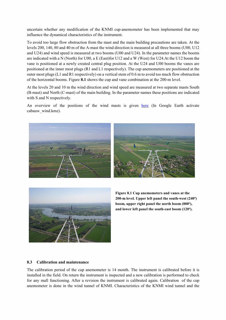
To avoid too large flow obstruction from the mast and the main building precautions are taken. At the levels 200, 140, 80 and 40 m of the A-mast the wind direction is measured at all three booms (U00, U12 and U24) and wind speed is measured at two booms (U00 and U24). In the parameter names the booms are indicated with a N (North) for U00, a E (East)for U12 and a W (West) for U24.At the U12 boom the vane is positioned at a newly created central plug position. At the U24 and U00 booms the vanes are positioned at the inner most plugs (R1 and L1 respectively). The cup anemometers are positioned at the outer most plugs (L1 and R1 respectively) on a vertical stem of 0.6 m to avoid too much flow obstruction of the horizontal booms. Figure 8.1 shows the cup and vane combination at the 200-m level.

At the levels 20 and 10 m the wind direction and wind speed are measured at two separate masts South (B-mast) and North (C-mast) of the main building. In the parameter names these positions are indicated with S and N respectively.

An overview of the positions of the wind masts is given here (In Google Earth activate cabauw_wind.kmz).

Figure 8.1 Cup anemometers and vanes at the 200-m level. Upper left panel the south-west (240o) boom, upper right panel the north boom (000o), and lower left panel the south-east boom (120o).

8.3 Calibration and maintenance

The calibration period of the cup anemometer is 14 month. The instrument is calibrated before it is installed in the field. On return the instrument is inspected and a new calibration is performed to check for any mall functioning. After a revision the instrument is calibrated again. Calibration of the cup anemometer is done in the wind tunnel of KNMI. Characteristics of the KNMI wind tunnel and the

application for calibration are described by Wieringa (1968) and by Monna (1983). A calibration results in a calibration factor (sensitivity) an offset and a threshold velocity. The WMO requirement of an accuracy of 0.5 m/s is met. In fact accuracy is better characterized by the largest of 1% or 0.1 m/s. The threshold velocity is better than 0.5 m/s. When these values are not met the instrument is rejected.

The calibration period of the wind vane is 26 month. Revision of the wind vanes consist of mechanically balancing and of testing the code disk directions. No dynamical calibration in the wind tunnel takes place. The WMO requirement of 3o is met. The orientation of the code disk is much better than this 3o. The vane blades undergo an on eye inspection of its flatness. At this stage it is uncertain what the influence of non-flatness is on the wind vane orientation. Relevant documents in KMS are:

• Calibratie uitrichtapparaat windvanen (pdf, KNMI-only, in Dutch)

• IJken windvanen (pdf, KNMI-only, in Dutch)

• Windvaan onderhoud (pdf, KNMI-only, in Dutch)

• Windvaan KNMI verwisselen (pdf, KNMI-only, in Dutch)

The azimuth of the wind vane plugs at the tip of the booms are determined with a camera relative to distant objects at close to the horizon. Relevant documents in KMS are (in Dutch, KNMI-only):

• Vaanplug richtcamera kalibreren (pdf, KNMI-only, in Dutch)

• Uitrichten vaanpluggen (pdf, KNMI-only, in Dutch)

8.4 Data logging

The instruments are logged with the KNMI wind SIAM (documentation, pdf, KNMI only, in Dutch). For wind speed a 3 sec running mean is calculated with an update frequency of 4 Hz. From this the 10 minute mean, gust, minimum and standard deviation are derived. Wind direction statistics are based on a 4 Hz sampled time series.

8.5 Corrections

For each 10 minute interval instruments are selected that are best exposed to the undisturbed wind. Even for the best exposed instruments some flow obstruction remains due to the presence of the tower and the supporting booms. Corrections at the 200, 140, 80 and 40 m level are applied according to Wessels (1983). These corrections depend on the plug position of the instrument. Obstruction around the B-mast differ from that around the A-mast. Measurements at the 20 and 10 m level performed in the B-mast are also corrected for flow obstruction. Corrections in the wind speed are typically 3% and corrections in wind direction are typically 3o. Flow obstruction corrections are also applied on the standard deviation of wind speed, the standard deviation of wind direction and on the wind gust. Some uncertainty in the wind gust remains because the wind direction at the moment of the gust may be different from the mean wind direction used to calculate the correction. Also dynamical effects of quickly changing wind direction on the wake of the tower may introduce uncertainties in the correction. Minimum wind speed, minimum wind direction and maximum wind direction are not corrected for flow obstruction.

8.6 Post Processing

The original wind speed and wind direction data of all wind sensors are archived (mean, sdv, max, min) together with the flow corrected values. For each level the value of the best exposed sensor is used for the wind parameter at a given height. The procedure to find the best exposed sensor is described in van der Vliet (1998, p45-46, in Dutch).

8.7 Data sets

10 minute values of the selected and corrected data (parameter values) are available from the CESAR database in the dataset cesar_tower_meteo. Original data and flow corrected data on a 10 minute basis are archived in the MOBIBASE dataset caboper starting at 20000321 for the levels 200, 140, 80 and 40 m. From 20000706 onward observations at all levels are available. From 20050610 onward 1 minute data are archived in the MOBIBASE dataset cabkmds. 12 second values can be extracted from the caboper sample files for the period starting at 20130101.

8.8 Quality checks

Automatic quality checks are performed by the KNMI wind SIAM (documentation, KNMI only). After each month all wind observations are displayed and an on-eye inspection takes place. Further tests on the performance of the sensors in the field are done by using redundancy in the wind observations.

8.9 Compare wind directions at one level

Graphs described in this section are displayed here.

At each level in the A-mast (200, 140, 80 and 40 m) three wind vanes are available. . For each month and for each level we plot the difference of the wind direction (U12 – U00, U24 – U12, and U00 - U24) as a function of wind direction. These plots are used to detect deviations from the normal influence of flow obstruction due to the mast, boom and the neighbouring cup anemometer. The distribution of the data points show a symmetric spread around the line that bisects the boom directions.

To monitor the observations over time we may select a specific wind direction interval and calculate for each month the mean wind direction difference. Here we select the wind direction interval with its centre at the bisect of the two boom directions. The advantage is that here the data are at a parabolic minimum, which makes the result relatively insensitive to the precise distribution of the data points within this wind direction interval. At this symmetry line we may expect that the deviations in observed wind directions due to flow obstruction are equal in magnitude but opposite in sign. For the current configuration the deviation in wind direction at the symmetry line is +2o for the boom with the largest direction, and -2o for the boom with the smallest direction. For the difference we expect -4o.

In the graph in section 2 we observe that over time smaller and larger changes in wind direction have occurred. Often these changes come in the form of jumps at moments that a vane is exchanged. When a jump is larger than 2o action is taken.

Note that with this test we can only say something about the relative orientation of the various vanes, not about the absolute orientation.

To investigate the small jumps in observed wind directions after wind vane replacements we started in 2016 with an additional control in the field. Each time a vane is replacement the orientation of the plug is determined. Just prior to the start of this new control program the KNMI instrumental department had, independently, already decided to replace the vane blade of each vane before it is put in the field. The results until now are:

Position Date Plug Vane Date Plug Vane

200 - 000

200 - 120

200 - 240

140 - 000 20160307 Oke -0.5

140 - 120

140 - 240

080 - 000

080 – 120 20160307 Oke -2.0

080 – 240 20160307 Oke -1.0

040 - 000

040 - 120 20160307 Oke +1.0

040 - 240

Table 2 Plug orientation and jump in observed wind direction after replacement of wind vanes in the A tower.

8.10 Compare wind speeds at one level

Graphs described in this section are displayed here. At each level in the A-mast (200, 140, 80 and 40 m) two cup anemometers are available. For each month and for each level we plot the ratio of the

wind speed (U00 / U24) as a function of wind direction. These plots are used to detect deviations from the normal influence of flow obstruction due to the mast and the neighbouring wind vane. We can

follow the relative sensitivity of the cup anemometers by selecting data from a specific wind direction sector and determine, on a monthly bases, the mean ratio. When the wind direction is along the

symmetry line between two booms we may expect that the deviations in observed wind speeds are equal and thus the ratio between the two should be 1.00. This idea is exploited by selecting data with: a) wind speeds larger than 3 m/s, which gives a well-defined wind direction and a well-defined wind

speed ratio; b) wind direction between -30 and +30o deviation from the symmetry line direction (310o). We observe that the influence of the flow obstruction is an anti-symmetric function of Δφ, the

angle between the wind direction and the symmetry line. A regression is performed of the form:

( )3310 ϕϕ ∆⋅+∆⋅+= aaaFratio (8.1)

Where Fratio is the wind speed ratio. The offset (a0) is now the monthly estimate for the wind speed ratio, and is plotted as function of time.

In the graph in section 2 we observe jumps which sometimes are related to the exchange of a cup anemometer. At other occasions there is a gradual drift in the wind speed ratio. When the ratio comes outside of the range [0.99:1.01] action is taken.

Note that with this test we can only say something about the relative sensitivity of the various cup anemometers, not about the absolute accuracy.

8.11 Treshold sensitivity of the wind vane

According to WMO and ICAO regulations the wind direction should be reported accurately when the wind speed is larger than 2 m/s (Handboek waarnemingen H5, H5.2.3, in Dutch ). Typical threshold wind speeds for vanes to respond are below 1 m/s (Monna, 1978, H4.5). The behaviour of the KNMI wind vanes at Cabauw were analysed for a low wind speed situation at 13-dec-2015 and maximum threshold speeds of 1.0 m/s were found for some of the vanes (see cleaning specials number 16).

8.12 Non-standard situations during operation

Period Parameter Issue Correction

20080213 - 20130424 F140 U24 Stem is missing No

20090909 – 20110321 D040-U12 Misalignment plug +12o

20110328 – 20120323 D140-U24 Misalignment plug -4.2o

201210 – 201305 F140-240o 2% deviation in ratio No, no cause found, calibrations oke.

20121010 D200-120o Misalignment plug +1.4o

201407 – 201503 F040 > 1% deviation in ratio No, cause could be traced to a specific cup-anemometer

8.13 Open issues

Jumps in wind vane orientation may occur when the vane plug changes orientation while tightening the nut of the vane on the plug. . Another reason may be deformation of the vane blade. Subjects that are currently (25-jun-2015) under investigation.

8.14 References

Monna WAA (1983). De KNMI windtunnel. KNMI Technical Report 32. Monna WAA (1978). Comparative investigation of dynamic properties of some propeller vanes. KNMI

Scientific-Report 78-11. Van der Vliet JG (1998). Elf jaar Cabauw metingen. KNMI Technical report 210. (in Dutch) Wessels HRA (1983). Distortion of the wind field by the Cabauw meteorological tower. KNMI Scientific Report

83-15. Wieringa J (1967). Evaluation and design of wind vanes. J. Appl. Meteorol., 6, 1114-1122. Wieringa J (1968). Nauwkeurigheid van anemometerijkingen in de KNMI windtunnel. KNMI-Verslag-211

9 Air temperature and dewpoint temperature In the definition phase of the observational program at Cabauw for 2000 and following years it was specified that the basic meteorological parameters should be measured with the same instruments as

used in the NL network of automatic weather stations. For humidity this meant that the accuracy was not good enough to resolve the structure of the humidity profile along the 200-m tower. In 2010 a project was started to improve the accuracy of the humidity observations. This resulted in 2014 in the introduction of new sensors (EE-33) and the increase of the frequency of sensor calibration.

9.1 Temperature and Humidity parameters

Temperature is measured at eight and Humidity is measured at seven levels.

Parameter Unit Description Period CESAR dataset MB dataset

TA200 degC Air temperature at 200 m 200005 - now tower_meteo caboper

TA140 degC Air temperature at 140 m 200005 - now tower_meteo caboper

TA080 degC Air temperature at 80 m 200005 - now tower_meteo caboper

TA040 degC Air temperature at 40 m 200005 - now tower_meteo caboper

TA020 degC Air temperature at 20 m 200005 - now tower_meteo caboper

TA010 degC Air temperature at 10 m 200005 - now tower_meteo caboper

TA002 degC Air temperature at 1.5 m 200005 - now tower_meteo caboper

TA000 degC Air temperature at 0.1 m 20130809 - now tower_meteo caboper

TD200 degC Dew point temperature at 200 m 200005 - now tower_meteo caboper

TD140 degC Dew point temperature at 140 m 200005 - now tower_meteo caboper

TD080 degC Dew point temperature at 80 m 200005 - now tower_meteo caboper

TD040 degC Dew point temperature at 40 m 200005 - now tower_meteo caboper

TD020 degC Dew point temperature at 20 m 200005 - now tower_meteo caboper

TD010 degC Dew point temperature at 10 m 200005 - now tower_meteo caboper

TD002 degC Dew point temperature at 1.5 m 200005 - now tower_meteo caboper

Time series are reduced to 10 minute values. Each parameter consists of four variables i.e: Mean value, standard deviation, maximum value, and minimum value, denoted with the names:

Variable Description CESAR dataset MB dataset

<parameter> Mean value tower_meteo caboper

S<parameter> Standard deviation caboper

P<parameter> Maximum value caboper

M<parameter> Minimum value caboper

9.2 Instruments and set-up

The instruments at the highest 4 levels are positioned at the south-east booms of the A-mast. The instruments at 10 and 20 m are positioned in the B-mast. The 1.5-m and 0.1-m instruments are positioned at the Meteo-field.

(200005 - 201004) The Air temperature is measured with a KNMI Pt500-element in an unventilated KNMI temperature hut. Dew point temperature is measured with a Vaisala HMP243 heated relative humidity sensor with a metal filter in a separate Vaisala unventilated hut. This hut is open in construction.

(201004 - 2014) Air temperature and humidity are measured in one unventilated hut, which consists of two compartments on top of each other. In the lowest compartment air temperature is measured with a EPLUSE Pt1000 element. In the upper compartment dew point temperature is measured with a heated EPLUSE 33 polymer sensor. At the 2-m level the temperature and dew point sensor remain situated in two separate huts adjacent of each other. The reason being that close to the surface vertical gradients can be significant over the depth of the hut. Various improvements on the dew point sensors has been performed in cooperation with the manufactory.

(20130809 – now) Air temperature at 0.1 m is measured with a KNMI Pt500-element in a special unventilated hut

(2014 – now) A design has been implemented of the EPLUSE 33 dew point sensor with improved electric shielding and coating.

9.3 Calibration, maintenance and accuracy

Temperature

Calibration is done at KNMI. Temperature sensors are calibrated in a well-steered deep alcohol bath. Temperature sensors are replaced each 38 month. Accuracy is 0.1 degC. Resolution is 0.1 degC.

Humidity

Humidity sensors are calibrated in a climate chamber against a dew-point mirror sensor. Dew point sensors are subject to contamination and drift of calibration. This makes it necessary to replace them more often.

(20005 – 201004) Replacement and calibration of the dew points sensors each 8 month. Accuracy is 3.5% RH. Resolution is 0.1 degC.

(201004 – 2014) Replacement and calibration of the dew points sensors each 3 month. Accuracy is 3.5% RH. Resolution is 0.1 degC. This is a test period to learn what calibration period is needed to obtain a significant better accuracy than before.

(2014 – now) Replacement and calibration of the dew points sensors each 3 month. Accuracy is 1.5 % RH. Resolution is 0.1 degC. Two batches of 7 Cabauw specific sensors are available which are always interchanged at the same time. This is to minimize differences due to drift in the field. Each batch consists of 4 electrically shielded sensors to be used in the A-mast (40, 80, 140 and 200m). This is for lightning protection. And three sensors not shielded to be used in the B-mast (2, 10 and 20 m). For both

the shielded and the unshielded are available one spare sensor. When a sensor fails, the spare sensor is used and the defect sensor is repaired if possible. The spare sensor is not allowed to have a last calibration longer than 3 moth ago at the moment of regular (3 month) replacement. If that would be the case, the spare sensor is first calibrated before it is placed in the field. In principle the original batch is in place when after more than 3 month they are replaced again in the field. But when repair takes more time, the spare sensor is used instead.

9.4 Performance and accuracy

The use of unventilated huts, compared to ventilated configurations, keeps maintenance to a minimum and is less prone to discontinuities in the observations. However, at conditions with low wind speed and high irradiation this configuration may result in overestimations of the air temperature of a few 0.1 degC (Meijer, 2000, pdf).

The humidity sensor often overestimates during drying episodes after dew, fog or rain, because of a wet shielding or sensor. This may result in observed dew point temperatures higher than the air temperature. Heating of the sensor, the change to metal filters and the open hut improves the functioning during high humidity conditions relative to older version of the Vaisala sensors. With the introduction of the EE-33 sensors an even better performance is achieved.

9.5 Datalogging

Data logging is done with the KNMI XU2-SIAM Temperatuur/Vocht HMP243 (documentation, pdf, KNMI only). From this the 10 minute mean, maximum, minimum and standard deviation are derived. With the introduction of the EE-33 sensors a new type of temperature/humidity SIAM was designed.

9.6 Corrections

No corrections

9.7 Post Processing

No post processing

9.8 Data sets

10 minute values of temperature and dew point for the levels 2, 10, 20, 40, 80, 140 and 200 m are available from the CESAR database in the dataset cesar_tower_meteo. 10 minute values of temperature and dew point for the level 2 m and temperature at 0.1 m are available from the CESAR database in the dataset cesar_surface_meteo.

9.9 Quality checks

Automatic quality checks are performed by the KNMI temperature SIAM (documentation, pdf, KNMI only). When fatal status codes are generated by the SIAM the operational service takes appropriate measures. After each month all temperature and humidity observations are visualized and an on-eye inspection takes place. Erroneous data are flagged and if necessary appropriate measures are taken.

9.10 Open issues

Calibration is done at KNMI against a dew point mirror instrument. This means that at dewpoints above 0 oC the value is against water and below 0 oC it is against ice (frost point temperature). When

converting dew point temperatures to absolute humidity one has to use the two different Magnus formulas for water and ice for dew points above and below 0 oC respectively. Specific humidity

Specific humidity is derived from dew point temperature and air pressure. Air pressure at height z above the surface is calculated from the observed surface pressure by adding 0.125*z hPa, where z is in meters.

9.11 Literature

Meijer EMJ (2000). Evaluation of humidity and temperature measurements of Vaisala"s HMP243 plus PT100 with two reference psychrometers. KNMI technical report 229.

10 Short wave radiation Short wave and longwave upward and downward radiation at the surface are measured at Cabauw. These observations are specifically done for the monitoring of land-atmosphere interaction at Cabauw. They differ from Cabauw BSRN observations in that the time series goes further back in time and that also upward fluxes are observed. Quality of the observations has improved over time and are currently close to BSRN standard.

10.1 Short wave radiation parameters.

CESAR MB Unit Description Period CESAR dataset MB dataset

SWD SWD W m-2 Short wave downward radiation MF: 200005 –

20121031

EB: 20121101 - now

surface_radiation

surface_meteo caboper

SWDMF W m-2 Short wave downward radiation 20000413 - 20130516 caboper

SWDEB W m-2 Short wave downward radiation 20110330 -now bsrncab

SWU SWU W m-2 Short wave upward radiation 200005 - now surface_radiation caboper

SWUMF W m-2 Short wave downward radiation 20000419 - 20130516 caboper

SWUEB W m-2 Short wave downward radiation 20110330 -now bsrncab

SWDTP W m-2 Short wave downward radiation

at 213 m

201209 - now surface_radiation bsrncab

10.2 Instruments and set up

[SWDMF][SWUMF]

Short wave upward and downward radiation are measured at the meteo field south of the A-mast at 1.5 m height. The two sensors are positioned 4 m apart. The downward looking sensor (albedo) is on a boom of 1 m length. The porting structure is painted black to get a well-defined radiation condition. Since December 2002 the instruments are ventilated and heated to avoid formation of dew, snow and rime. The instruments are Kipp&Zn CM11 pyranometers.

The instruments have small offsets ( a few W m-2) due to long wave cooling. This results in negative values during night time. These values are set to zero. Note that this negative offset is also present during daytime and will result in a systematic bias.

[SWDEB][SWUEB]

Short wave upward and downward radiation are measured at the energy balance field. The instruments are mounted at 1.5 m height at the same position, and at the same position as the long wave instruments [LWDEB][LWUEB]. The instruments are Kipp&Zn CM22

pyranometers, which are of the same type as used at the Cabauw BSRN site. The instruments are heated and ventilated to avoid formation of dew, snow and rime formation at the domes. Ventilation also helps to reduce the influence of long wave cooling.

[SWD][SWU]

The MF and EB are merged.

[SWDTP]

For the fog observational program a ventilated and heated Kipp&Zn CM22 pyranometer is installed at the top of the A-mast. To reduce interference with the drizzle radar (IDRA) at the top of the mast, the sensor is installed on a boom extended 2 m to the south from the top platform at 213 m height.

The boom is mounted along the fence at the east side of the top plateau and can be pulled inward along the fence for maintenance. Leveling of the instruments and controlling this leveling is not straight forward, because the inclinometers cannot be seen when the boom is extended into the measuring position. To establish a level mounting the boom with instruments is mounted temporarily along the fence 2 m to the north east, in such a way that the instruments inclinometers can be seen. The instruments were than adjusted to the horizontal plane. Then, the whole boom configuration was moved along the fence to its final position at the south tip of the plateau. A check was performed to assure that the two fence segments used for the mountings where parallel. At this stage no regular check is performed on the leveling of the instruments.

10.3 Calibration and maintenance

[SWDMF][SWUMF] The CM11 sensors are calibrated at KNMI against a reference instrument which itself is calibrated at the World Radiation Center in Davos (Switzerland).

[SWDEB][SWUEB] The CM22 sensors are calibrated directly at the World Radiation Center in Davos (Switzerland).

The domes of the instruments are cleaned once a week.

10.4 Data logging and processing

[SWDMF][SWUMF] Data logging of the CM11 pyranometers is done with the KNMI XQ1/XD0/XF0-SIAM for radiation with a sampling rate of 12 s. Negative values which occur during nights with long wave cooling are set to zero.

[SWDEB][SWUEB][SWDTP] Data logging of the CM22 pyranometers is done with the KNMI-BSRN Q-SIAM and KNMI-BSRN T-SIAM for radiation with a sampling rate of 1 s. Negative values which occur during nights with long wave cooling are retained.

For the parameters [SWD] and [SWU] the data of the first period [SWDMF][SWUMF] and of the second period [SWDEB][SWUEB] are merged into one time series.

10.5 Non-standard situations

At the 16th of January 2003 the albedo instrument [SWUMF] was moved some 12 m to the West, distance from SWDMF now 8 m. The reason being the presence of a small ditch in the field of view of the instrument which could reflect direct sunlight into the instrument. This became particularly obvious during a cold spell period with ice forming in the ditch. At this new location a small depression in the field close to the albedo instrument was present in which surface water could form during very wet episodes. At the 10th of February 2003 the grass around the new location was removed, soil was applied and the grass was replaced again. At the start of the growing season the surface at the albedo location rapidly became the same as its surroundings.

When the first observations at the energy balance field started in 2011 the underlying terrain was not representative for the grass land at Cabauw due to the ground manipulation at build up time. Thus SWDEB data are not representative during this first stage. During 2012 it was found that the radiation poles at the meteo field were eroded and the instruments there had to be removed. This resulted in the transition from MF to EB observations in the merged time series at the start of 201211.

The short wave radiation observations at the energy balance field suffer from occasional

10.6 Quality checks

Automatic quality checks are performed by the KNMI temperature SIAM (documentation, pdf, KNMI only) After each month all short wave radiation observations are visualized and an on-eye inspection takes place. Erroneous data are flagged and if necessary appropriate measures are taken.

More subtle changes in the instruments are monitored on a monthly basis by: 1) Comparing with the BSRN observations, and 2) Looking at the zero offset and its relation with net long wave cooling.

11 Long wave radiation Longwave upward and downward radiation at the surface are measured at Cabauw. These observations are specifically done for the monitoring of land-atmosphere interaction at Cabauw. They differ from Cabauw BSRN observations in that the time series goes further back in time and that also upward fluxes are observed. Quality of the observations has improved over time and are currently close to BSRN standard.

From the long wave upward radiation an estimate of the surface (skin) radiative temperature can be derived through Stefan-Boltzmann law. A correction for reflected down ward long wave radiation may be applied given that the emissivity of the surface is less than 1.00. The emissivity of the grassland at cabauw has never been measured, literature values range from 095 -1.00, 0.97 may be a reasonable value. See also Chapter 13 on radiative temperatures.

11.1 Long wave radiation parameters

CESAR MB Unit Description Period CESAR dataset MB dataset

LWD LWD W m-2 Long wave downward radiation 200005 - now surface_radiation caboper

LWDMF W m-2 Long wave downward radiation 20000609 - 20121106 caboper

LWDEB W m-2 Long wave downward radiation 20110805 - now bsrncab

LWU LWU W m-2 Long wave upward radiation 200005 - now surface_radiation caboper

LWUMF W m-2 Long wave upward radiation 200005 - 201210 caboper

LWUEB W m-2 Long wave upward radiation 201104 -now bsrncab

LWDTP W m-2 Long wave downward radiation

at 213 m

201209 - now surface_radiation bsrncab

11.2 Instruments and set-up

[LWDMF][LWUMF]

Long wave upward and downward radiation are measured at the meteo field South of the A-mast at 1.5 m height. The sensors are on a boom of circa 1 m length. The instruments are mounted in one housing to assure equal house temperatures. They are ventilated to avoid formation of dew, snow and rime and to minimize heating of the domes through irradiation. The domes are equipped with small thermistors. Corrections are applied for heating of the domes. The instruments are Eppley pyrgeometers (PIR). Calibration is done at the World Radiation Center in Davos (Switzerland).

[LWDEB][LWUEB]

Two pyrgeometers were installed at the energy balance field to measure long wave downward and upward radiation. The instruments are mounted at 1.5 m height at the same position, and at the same position as the short wave instruments [SWDEB][SWUEB]. The instruments are Kipp&Zn CG4 pyrgeometers, which are of the same type as used at the Cabauw BSRN site. The instruments are heated and ventilated to avoid formation of dew, snow and rime formation at the domes. Ventilation also helps to decrease the temperature difference between the domes and the house. These instruments don’t need corrections for dome temperature.

[LWDTP]

For the fog observational program a ventilated and heated Kipp&Zn CG4 pyrgeometer was installed at the top of the A-mast. To reduce interference with the drizzle radar (IDRA) at the top of the mast, the sensor was installed on a boom extended 2 m to the south from the platform.

11.3 Measurement principle

The pyrgeometer contains of a housing and a horizontal sensor surface which is exposed to the electro-magnetic radiation of the hemisphere. The sensor surface is thermally coupled to the housing by material with a well-defined heat conduction coefficient. An optical filter assures that only infrared radiation in the range 4.5 – 50 µm is passed to the sensor surface. The net radiation of the sensor surface will be balanced by the conductive heat exchange with the housing. The instrument measures the temperature of the housing and the difference between the housing and the sensor surface. Given the heat conduction coefficient between the sensor surface and the housing, the latter is thus a measure of the difference of

the long wave radiation emitted by the sensor surface and the long wave radiation received by the sensor form the hemisphere. Together with the housing temperature and by applying the Stefan-Boltzmann law for black body radiation the incoming thermal radiation can be derived.

Keeping temperature differences between sensor surface, dome and housing helps for obtaining accurate measurements. This can be accomplished by ventilation and/or by shading the instrument against direct solar light. Some instruments measure the dome temperature, which allow for corrections.

11.4 Data logging and processing

[LWDMF][LWUMF] Data logging for the Eppley pyrgeometer is done with the KNMI XL0-SIAM (documentation, pdf, KNMI only) for Eppley radiation with a sampling rate of 12 s.

[LWDEB][LWUEB][LWDTP] Data logging for the Kipp&Zn pyrgeometer is done with the KNMI-BSRN Q and KNMI-BSRN T-SIAM for radiation with a sampling rate of 1 s.

For the parameters [LWD] and [LWU] the data of the first period [LWDMF][LWUMF] and of the second period [LWDEB][LWUEB] are merged into one time series.

11.5 Non-standard situations

(Added 09-nov-2007) Doubts exists about the reliability of the long wave downward radiation. A number of scientists, who compared the long wave downward radiation observations with their radiation transport models, reported significant deviations. Currently a comparison is performed between the PIR and new instruments from the Cabauw BSRN station. The preliminary conclusion is that the PIR overestimates long wave downward radiation. It appears that the sensitivity of the sensor (which measures the difference between the black body radiation of the housing of the instrument and the long wave downward radiation) is 10% smaller then assumed. A correction of 10% has been applied to the data.

(Added 09-nov-2007) After a replacement of the data logger of the instruments around the 20th of June 2007 the long wave downward radiation shows an extra offset of circa +7 W/m2. Further investigations revealed problem in the design of this specific SIAM data logger. The offset appears to be stable over time. A correction of 7 W m-2 has been applied.

In December 2012 it was found that during rainy episodes LWUEB occasionally gave unexpected values. The instrument is positioned upside down, and it was found that water was trapped in the white shielding of the instrument. A small hole was drilled to allow for the drainage of rain water.

11.6 Quality checks

Automatic quality checks are performed by the SIAM. After each month all long wave radiation observations are visualized and an on-eye inspection takes place. Erroneous data are flagged and if necessary appropriate measures are taken.

More subtle changes in the instruments are monitored on a monthly basis by: 1) Comparing with the BSRN observations, and 2) deriving the sensitivity for short wave radiation.

12 Net radiation

12.1 Net radiation parameters

CESAR MB Unit Description Period CESAR dataset MB dataset

QNET W m-2 Net radiation 20020725 - 20121214 caboper

CRD W m-2 Total wave downward radiation

corrected

20020725 - 20121214 caboper

CRU W m-2 Total wave upward radiation

corrected

20020725 - 20121214 caboper

RD W m-2 Total wave downward radiation 20020725 - 20121214 caboper

RU W m-2 Total wave upward radiation 20020725 - 20121214 caboper

QNBAL QNBAL W m-2 Net radiation from balance 200005 - now surface_radiation caboper

SWD W m-2 Short wave downward radiation 200005 - 201210 caboper

LWD W m-2 Long wave downward radiation 201104 -now bsrncab

SWU W m-2 Short wave upward radiation 200005 - 201210 caboper

LWU W m-2 Long wave upward radiation 201104 -now bsrncab

12.2 Instruments and set-up

[QNET]

Net radiation is measured at the meteo field south of the main tower at 1.5 m height. The sensor is positioned at a boom of 0.8 m. The instrument is a Schulze net radiometer type LXG055 (Schulze-Daeke type). The instrument measures the total, long and short wave, downward radiation [RD] and the total upward radiation [RU] separately. The instrument is ventilated and heated to prevent dew formation and to keep temperature differences small. Net radiation is derived by taking the difference of the downward and upward components.

[QNBAL]

Net radiation is derived from the budget of the four components [SWD], [SWU], [LWD] and [LWU].

12.3 Calibration and maintenance

[QNET] Calibration of the short wave sensitivity is done at KNMI.

12.4 Data logging and processing

[QNET] Data logging is done with KNMI XL1-SIAM for Schulze (document, pdf,KNMI-only).

12.5 Quality checks

Automatic quality checks are performed by the KNMI XL1-SIAM for Schulze (documentation, pdf, KNMI only) After each month all long wave radiation observations are visualized and an on-eye inspection takes place. Erroneous data are flagged and if necessary appropriate measures are taken.

More subtle changes in the instruments are monitored on a daily basis by comparing sensitivities for long and short wave radiation, both for upward and downward components, with the instruments for the individual radiation components. The following regression coefficients are used:

CSWDBXLWRDAXLWRD +⋅+−⋅=− )(

CSWUBXLWRUAXLWRU +⋅+−⋅=− )(

Where XLW is the black body radiation of the Schulze housing which is added to the sensor value to arrive at total radiation. A, B, and C are regression coefficients.

For the downward component the range in the long wave component is

13 Radiative temperature Radiative temperature observations are closely related to the observation of long wave radiation flux. But where the latter is broad band and hemispheric (the total flux through a surface) to obtain an energy flux, the radiative temperature instrument measures radiation fluxes in a smaller spectral band and in a smaller solid angle by collimation of the infrared light. This enables the remote measurement of the temperature of a specific object, by choosing a spectral band where the influence of radiation from the atmosphere between sensor and object can be neglected. The same instrument can be used to detect the presence of clouds by exploiting the contrast in radiation temperature of the cloud ceiling and the clear sky. The influence of emissivity’s less than 1.00 has not been investigated so far.

13.1 Radiative temperature parameters

CESAR MB Unit Description Period CESAR dataset MB dataset

TIRUH degC Radiation temperature EB-files

from A-mast 200 m level

20010914 - now

cabsurf

TIRUL degC Radiation temperature Soil-plot 20010908 - now cabsurf

TIREB degC Radiation temperature from

long wave upward EB-field

20110908 - now

cabsurf

TIRDA degC Radiation temperature sky

zenith

20021112 - now

cabsurf

TIRDB degC Radiation temperature sky

zenith

20021112 -20110906

cabsurf

TGND1 degC Radiation temperature

Nubiscope surface east ward

nubiscop

TGND2 degC Radiation temperature

Nubiscope surface west ward

nubiscop

13.2 Instruments and set-up

Here we use Heitronic KT15 instruments. They come in various type: small opening angle (K6, 30) or large opening angle (M6, 400), and wide band 8-14 µm and small band 9.6-11.5 µm, which gives more or less sensitivity to atmospheric moisture. The small band versions are preferably used when the distance to the object of interest is large.

In the early period there were doubts about the temperature stability of the sensor. Therefor the sensors are mounted in a housing and thermostated. Thermostat temperature is kept at 32 degC. When air temperatures rise above 25degC the housing temperature in general starts to increase.

Later it was judged that thermal stability had increased, and it was realized that accuracy of the measurements is better when the object temperature is close to the housing temperature. Therefor in the second period the sensors were not thermostated, but due to the housing and the heat produced by the instrument housing temperature is typically 10 degC above air temperature.

[TIRDA][TIRDB]

(200109) Cloud detection is done by upward looking pyrometers with small band spectral filter and small opening angle (KT15.85A, K6, 9.6-11.5µm, thermostated). The sensors are positioned at the remote sensing field. A rain detector triggers a shutter that protects the instrument against rain.

(20040305) [TIRDB] is moved to the wind profiler/RASS field for colocation.

(20110812) [TIRDA] instrument replaced by type KT15.85IIP (K6, 9.6-11.5µm, not thermostated)

(20110907) [TIRDB] discontinued

[TIRUH]

(20010914) Surface temperature of the grassland is measured with a sensor positioned at 206 m height in the A-mast looking downward in an easterly direction (azimuth and elevation not exactly known). The instrument is a KT15.85A (K6, 9.6-11.5µm,, thermostated) with a small field of view.

(20110812) The instrument is replaced with a KT15.IIP (M6, 9.6-11.5µm, thermostated) with a wide field of view and oriented north towards the energy balance field.

[TIRUL]

Surface radiation temperature of the grassland is measured at the meteo field (soil plot) from 2 m height looking vertically down. The instrument is a KT15.SMD (M6, 8-14µm, thermostated) with a wide field of view. (20140706) thermostat does not function anymore.

[TIREB]

Surface radiation temperature of the grassland is measured at the energy balance field (soil plot) from 2 m height looking vertically down. The instrument is a KT15.IIP (M6, 9.6-11.5µm, not thermostated) with a wide field of view.

[TGND1][TGND2]

A Nubiscope (KNMI report, pdf) is operational at the BSRN site. It performs sky hemispheric scan every 10 minutes. During this scan it also measures the surface radiative temperature of two land surface points. When the scan cycle has arrived at 90o azimuth, and at 270o one sample is taken at an elevation angle of -45o, resulting in TGND1 and TGND2 respectively.

(20180715 - ) [TGND2] The west ward land surface point has become more or less bare soil due to the continuing drought (photo east 03-Oct-2018) (photo west 03-Oct-2018). This results in a much higher variability and extreme high temperatures during sunny periods.

13.3 Calibration

(2001 – 201108) The instruments are calibrated in 2003 as reported by Kohsiek 2004 (document, pdf)

(201109- now) Except for the instrument at the meteo field [TIRUL] all instruments are now regularly calibrated.

13.4 Maintenance

The instruments optics are regularly cleaned. Since 2011 the procedure for cleaning has been described in ????.

13.5 Datalogging

In the first period Skipper loggers were used with memory cards. During 2002 the logging of the instruments was subsequently transferred to a PC with a Microstar DA-converter. (20110908) Logging is by the KNMI H-SIAM for pyrometers (documentation, pdf, KNMI-only)

14 Photo-active radiation Photo active radiation is the part of the visible and near-infrared light that plays a role in the photosynthesis of plants.

14.1 Photo-active radiation parameters

CESAR MB Unit Description Period CESAR dataset MB dataset

PARLIC W/m2 Upward photo-active radiation 20070221 - 20170523 bsrncab

14.2 Instruments and set-up

Upward photo active radiation has been measured by Alterra at the BSRN site. Instrument type is LICOR 190 SA.

15 Surface flux

15.1 Surface Energy Budget.

A general problem in micrometeorology is the observed imbalance in the surface energy budget. Typical imbalances are 15% during day time and up to 100% during night time. During stable atmospheric conditions the imbalance appears to be a function of wind speed. The lower the wind speed the larger the imbalance. A poster on this topic has been presented at the EMS 5th Annual Meeting, 12-16 sep 2005, Utrecht, The Netherlands.

15.2 Net radiation

Net radiation is derived from observations of the individual components of the surface radiation budget. A description and the data of the observations of the radiation budget can be found with the dataset: "cesar_surface_radiation".

15.3 Soil heat flux

Surface soil heat flux is derived from a combination of observations with soil heat flux plates and soil temperature needles. A description and the data of the observations of the soil thermal system can be found with the dataset: "cesar_soil_heat".

15.4 Turbulent surface fluxes

Turbulent fluctuations of wind, temperature, humidity and CO2 are measured with a combination of a sonic anemometer/thermometer (wind vector and sonical temperature) and an optical open path sensor (H2O and CO2). From this the vertical fluxes of momentum, sensible heat, latent heat and CO2 are derived by means of the eddy correlation technique.

Let wi be a sampled time series of the vertical wind speed and ci the quantity for which the vertical flux is to be determined. The average turbulent flux (Fc)for a given time period (T) in which N samples are acquired is then given by:

Fc=1/N*SUM((wi-<w>)*(ci-<c>)

Where <w> and <c> denotes the average values over the period T

Corrections

Corrections to the sonical temperature are applied for moisture and lateral wind. Humidity and CO2 fluctuations are corrected for density fluctuation induced by temperature and humidity fluctuations (Webb-correction). Wind fluctuations are corrected for streamline tilt due to flow obstruction around the supporting mast and instruments. Low frequency losses are corrected according to Bosveld (1999), this method is verified by Schalkwijk et al. (2010). No corrections for sensor separation and path averaging is applied until now. Comparing co-spectra of wt and wq for the current 3 m configuration shows a typical loss of 6% in wq due to the sensor separation between the sonic and the licor. Spectral losses in wt will be significantly smaller since the paths of the temperature and vertical wind observations coincide. (ongoing work)

Details and limitations of the eddy correlation technique have been described extensively in the open literature. A good introduction can be found in Xuhui Lee, W. J. Massman, Beverly E. Law (2004)

Uncertainties in flux estimates

There are several sources of uncertainty when looking at eddy-correlation flux estimates:

1. Uncertainty in corrections for spectral attenuation at the high frequency side

See Chapter 4 of Lee X., W. Massman and B. Law (2004). Handbook of micrometeorology: A guide for surface flux measurements and analysis. Atmospheric and Oceanographic Sciences Library. Kluwer Academic Publishers. ISBN 1-4020-2264 (HB); ISBN 1-4020-2265-4 (e-book).

but also the papers of:

Moore C. J. (1986). Frequency response corrections for eddy correlation systems. Boundary Layer Meteorology, 37, 17-35. and Moncrieff J. B., J. M. Massheder, H de Bruin, J. Elbers, T. Friborg, B. Heusinkveld, P. Kabat, S. Scott, H. Soegaard and A. Verhoef (1997). A system to measure surface fluxes of momentum, sensible heat, water vapour and carbon dioxide. Journal of Hydrology 188-189, 589-611.

Depending on the configuration corrections are typically around 5 %. And hopefully when the corrections are applied appropriately the remaing uncertainty is a few percent and may be systematic.

For an account on delay times in the instruments and datalogging of the period before 2007 click here

2. Uncertainty in corrections for spectral attenuation at the low frequency side

Chapter 5 of the Handbook of micrometeorology is devoted to this topic. Here we implemented a correction scheme described in Ch6 of The Garderen experiment. For measurements at low height the corrections are in general only a few percent. After correction maybe an uncertainty of 1 % remains.

3. random uncertainty due to the stochastic property of turbulence.

This is an easy one and described by Wyngaard in Ch 3.7 of the Workshop on micrometeorology, Hauden D. (ed.) (1973). Published by the American Meteorological Society. For a 10 minute averaged heat flux measured at z=3m, under convective conditions and with wind speed of 5 m/s this amounts to 10% random uncertainty. Uncertainty will be smaller when stability increases.

4. Representativity uncertainty, footprint under inhomogenuous conditions.

Very dependent on the situation, when fetch is ideal no problem.

5. Surface Energy Budget Closure.

Probably the biggest problem of them all and unsolved. At Cabauw imbalance is typically 10-15 % during day time and more during night time, Here is a link to a paper I wrote for the KNMI triennual on the status of SEB Closure at Cabauw. What can be done is use the Bowen ratio as measured by the eddy correlation system and distribute the available energy (=Net radiation minus- soil heat flux) over the two heat fluxes in proportion.

15.5 Additional fluxes

The sonic temperature flux cross wind corrected but without moisture correction is almost equal to the virtual temperature flux. The latter being proportional to the buoyancy flux as it appears for example in the calculation of the Obokhov stability length scale.

In Cabauw the local roughness length for momentum (3 cm) is much smaller then the regional scale roughness (0.15 cm). A friction velocity representative for the regional scale is derived from the observed 10 m wind and sensible heat flux based on regional roughness values published by Beljaars (1988), later reproduced in Beljaars and Bosveld (1997). Note that Verkaik and Holtslag (2007) published new results on roughness length at Cabauw which do not differ to much from the earlier findings.

Instruments

(20000801) The sonic anemometer is a Kaijo-Denki, probe type TR60-A, electronic unit DAT-300 or DAT-600. The sonic path is 0.2 m. Resolution is 0.1 K. The H2O/CO2-sensor is a KNMI Infrared Fluctuation Meter (IFM). Pathlength is 0.3 m. Resolution is 0.003 g/m3 H2O and 0.15 ppm CO2.

(20051101) IFM is replaced by LICOR 7500 Open path H2O/CO2 sensor

(20060913 – now) Kaijo Denki is replace by Gill R3 sonic anemometer/thermometer.

Configuration

(20000801) Turbulent surface fluxes are measured at 5 m height approximately 200 m South of the main tower . A sonic anemometer/thermometer is used to measure turbulent fluctuations of the three wind components and (sonical) temperature. The sonical temperature is measured along the vertical transducer pair. An open path infrared fluctuation meter is used to measure turbulent fluctuations of humidity and carbondioxide. The sonic anemometer has an azimuthal opening angle of 120o for horizontal wind measurements. The open path sensor is positioned vertically just behind the sonic probe at a distance of 0.3 m from the vertical sonical path. The instruments are mounted on a 1 m thin vertical cylinder to avoid a too strong flow obstruction due to the supporting mast. The vertical cylinder is supported by a rotator which is controlled by a wind direction tracking system and automatically turned into the mean wind direction each 2 hours. An inclinometer is positioned between the rotator and the supporting cylinder.

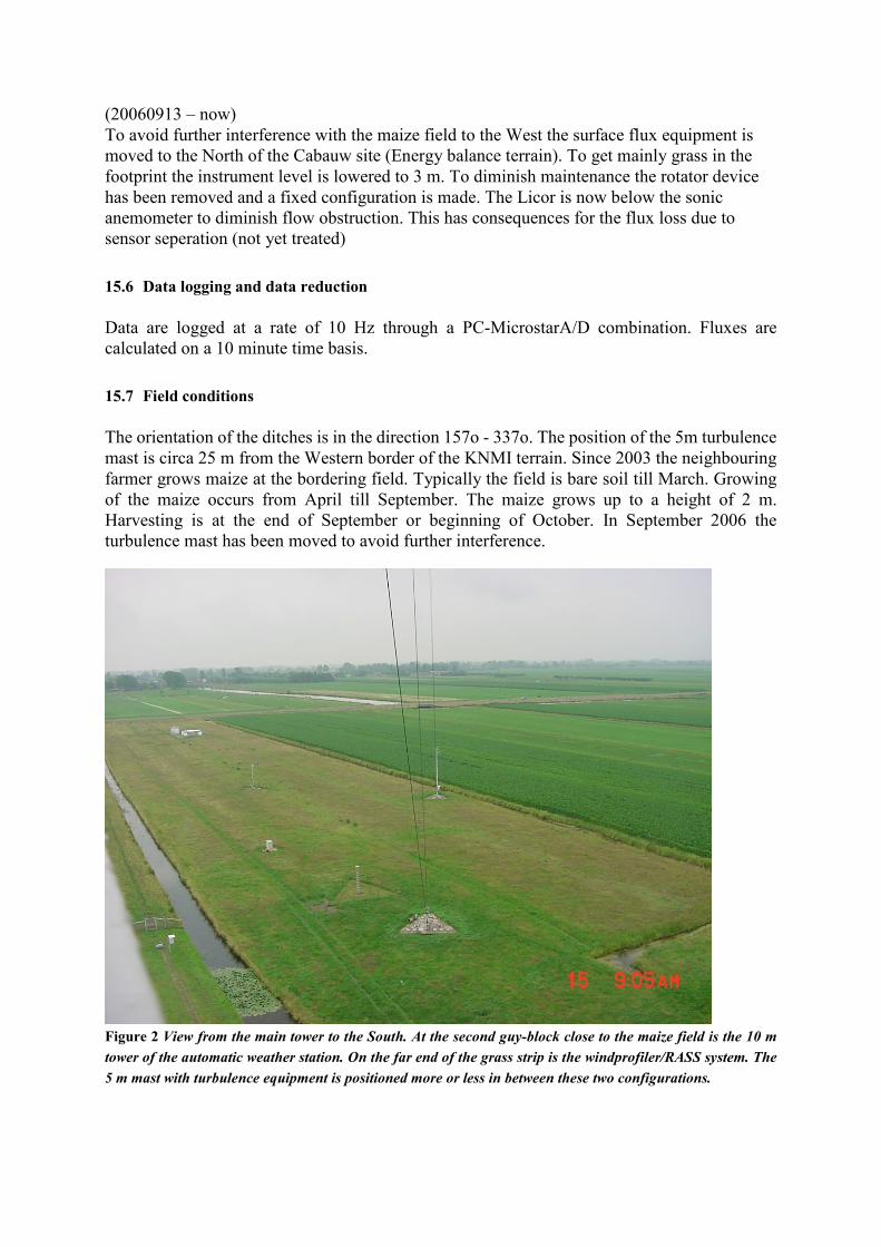
(20060913 – now) To avoid further interference with the maize field to the West the surface flux equipment is moved to the North of the Cabauw site (Energy balance terrain). To get mainly grass in the footprint the instrument level is lowered to 3 m. To diminish maintenance the rotator device has been removed and a fixed configuration is made. The Licor is now below the sonic anemometer to diminish flow obstruction. This has consequences for the flux loss due to sensor seperation (not yet treated)

15.6 Data logging and data reduction

Data are logged at a rate of 10 Hz through a PC-MicrostarA/D combination. Fluxes are calculated on a 10 minute time basis.

15.7 Field conditions

The orientation of the ditches is in the direction 157o - 337o. The position of the 5m turbulence mast is circa 25 m from the Western border of the KNMI terrain. Since 2003 the neighbouring farmer grows maize at the bordering field. Typically the field is bare soil till March. Growing of the maize occurs from April till September. The maize grows up to a height of 2 m. Harvesting is at the end of September or beginning of October. In September 2006 the turbulence mast has been moved to avoid further interference.

Figure 2 View from the main tower to the South. At the second guy-block close to the maize field is the 10 m tower of the automatic weather station. On the far end of the grass strip is the windprofiler/RASS system. The 5 m mast with turbulence equipment is positioned more or less in between these two configurations.

15.8 Calibration

Calibration of the sonic anemometer is done, approximately each second year, in a wind tunnel of TNO-Apeldoorn. Occasionally temperature calibrations has been performed at KNMI. H2O and CO2 calibration is performed in the field each year according to the calibration procedure provided by the manufacturer. Currently a calibration procedure for temperature, humidity and CO2 calibration is setup in the calibration laboratory at KNMI

15.9 Known Problems

Sonic temperatures were compared with the standard temperature observations at Cabauw. By regression for each day an estimate of the sensitivity of the sonic temperature was obtained. It was found that sensitivity was 0.97 before February 2003 after that sensitivity started to deviate till june 2004. After that the instrument was replaced and sensitivity was back to 1.00. Covariances with temperature are corrected according to the table below. For intermediate dates sensitivity values were interpolated.

date sensitivity

20000101 0.97

20030201 0.97

20030609 0.81

20040301 0.81

20040719 0.65

20040811 1.00

20491231 1.00

15.10 Quality Checks and processing

Data are archived near real-time in 10 minute intervals. This makes up the unvalidated dataset. After each month data are checked for completeness. Data are checked and flagged for malfunctioning by visualisation of time series. This make up the the validated dataset Data rejection mostly takes place under unfavourable conditions like rain and dew formation.

15.11 Parameters in CESAR database

A short description of each parameter is in the long_name attribute in the header of the NetCdf file (see below). For some parameters additional information is given here.

USTED Friction velocity derived from eddy-correlation observation close to the surface ( at 3 (after sep-2006) or 5 m (before sep-2006) height) It is derived from the component of the horizontal stress vector along the mean wind direction. The observations are corrected for streamline tilt and for low-frequency flux loss due to the finite averaging time of 10 minutes. The observations are representative for the local grass land which has a roughness length of approximately 0.03 m.

USTAB The same as USTED except that it is derived from the length of the horizontal stress vector. In general differences will be small except under convective low wind speed cases where USTED can become undefined.

USTPR is the friction velocity derived from the 10 m wind observations and the regional scale roughness length table as given in Beljaars and Bosveld (1997). Stability corrections are derived by using the sonic temperature heat flux as derived from the eddy-correlation observations close to the surface. This friction velocity is representative for the regional scale around Cabauw.

15.12 References

Beljaars A.C.M. (1988). The measurement of gustiness at routine wind stations. Paper presented at the WMO technical conference on instruments and methods of observation (TECO-1988). Leipzig, German Democratic Republic, 16-20 May 1988. Published in WMO Instruments and Observing Methods Report No. 33.

Bosveld F.C. (1999).The KNMI Garderen experiment, micro-meteorological observations 1988-1989: corrections. KNMI publication: WR-99-03.

Beljaars A.C.M. and F.C. Bosveld (1997). Cabauw data for the validation of land surface parametrization schemes. J. of Climate, 10, 1172-1193.

Schalkwijk, J., F.C. Bosveld and A.P. Siebesma (2010). Timescales and structures in vertical transport in the atmospheric boundary layer. KNMI publication: WR-2010-02.

Verkaik J.W. and A.A.M. Holtslag (2007). Wind profiles, momentum fluxes and roughness lengths at Cabauw revisited. Boundary Layer Meterology, 122, 3, 701-719.

Xuhui Lee, W.J. Massman, Beverly E. Law (2004). Handbook of micrometeorology: a guide for surface flux measurement and analysis.

16 Turbulence and turbulent fluxes

Eddy correlation fluxes are measured at three levels in the tower (60, 100 and 180m). At each level a sonic anemometer/thermometer and an open path H2O/CO2 sensor is installed at the South-East (130o) boom. With wind coming from 280 to 340 degrees mast interference is too large to obtain reliable observations. This wind sector should be excluded from any analysis. The open path sensors don't function properly during moist conditions (rain or dew).

Two types of sonic anemometers have been used over the years. The Kaijo Denki DAT 300 asymmetric probe has an obvious coordinate system with the main axis along the line of symmetry through the 120 degrees opening of the transducers. The positive direction is into this 120 degree opening angle. The Gill R3 probe has a frame with three spars in which the three transducer pairs are mounted. The probe has a 120 degree symmetry. One of the spars is indicated by a notch and the symbol N (North). The coordinate system can be configured in two ways. Either the main axis aligned along the N spar, with positive direction from the center to the N spar, or the main axis aligned along the first transducer pair. This is the transducer pair with an angle of 30 degrees relative to the N spar. The upper transducer is closest to the N spar, and the positive direction is from the center to this upper transducer. See drawing 1210-K-063 “R3 Anemometer U, V, W Axis Definition” in the manual. In our case the Gill R3 is always configured with the main axis along the first transducer pair.

16.1 Turbulence at 3/5 m

(20000801) Turbulence observations are performed 200 m south of the main tower at 5 m height. Instruments are a Kaijo Denki DAT 300 asymmetric sonic anemometer thermometer, and a home build H2O/CO2 open path sensor. The open path sensor is positioned behind the sonic anemometer and the combination is put on a rotor device which orients the sonic into the mean wind direction. Orientation is done each 2nd hour. Analogue data logging is performed.

(20060913) In the period 2004-2006 Maize was grown to the west of the turbulence mast. It was decided to move the turbulence mast to 200 m to the north of the main tower, where the instruments are exposed only to grassland. This movement was combined with a change of equipment. A Gill R3 symmetric version was combined with a Licor 7500 open path H2O/CO2 sensor. The instrument where placed at 3 m height. The rotor device has been removed. Therefor the open path sensor is positioned below the sonic measuring volume to avoid too much flow obstruction. Analogue data logging is performed.

(20160120) Gill R3 (user manual, pdf) is logged digitally. With this digital data stream comes various pieces of status information of the instrument. These pieces are packed in subsequent raw data records, and are continuously repeated. Part of the information is static in a given period, like anemometer type and anemometer configuration. Others are dynamic and indicate problems of the instruments like reduced transducer gain. Each piece is in an 8 bit word. Some of them are packed into 16 bits words.

MB Description GILL Address MB dataset

S1G<level> Error codes A00 cabturb3

S2G<level> Instrument configuration 256*A 01+A06 cabturb3

S3G<level> Data output configuration 256*A 03+A02 cabturb3

S4G<level> Transducer gain and errors 256*A 04+A05 cabturb3

AGC<level> Transmissivity of the optics cabturb3

Table 3 GILL R3 status codes as stored in MOBIBASE. GILL address refers to the status addresses A00 .. A06 as documented in the GILL R3 user manual section 7.1.3.

(20160120) Licor 7500A (user manual, pdf) is logged digitally. With this digital data stream comes status information. Most notably the transmissivity of the optics

16.2 Turbulence at 60 m

(20030813)

In cooperation with the USA-National Science Foundation turbulence instruments are operated in the main tower at 60 m height. Boom direction 120o. A Kaijo-Denki 20 cm path sonic anemometer/thermometer and a Licor open path infrared fluctuation meter are used to measure turbulent fluctuations of the three wind components, temperature, humidity and carbon dioxide. The instruments are mounted on a thin vertical cylinder to avoid a too strong flow obstruction of the supporting boom. An inclinometer is mounted between the instruments and the boom. Expected observational period: 13-August-2003 till 31-dec-2005.

(20061026) The Kaijo Denki is replaced by Gill R3 sonic anemometer.

(20160430) Reconfiguration of wiring and data logging, no observations

(20161110 - now) Observations resumed

16.3 Turbulence at 100 m

(20030523)

In cooperation with Alterra Wageningen turbulence instruments are operated in the main tower at 100 m height. Boom direction is 120o. A Solent 20 cm path sonic anemometer/thermometer and a Licor openpath infrared fluctuation meter are used to measure turbulent fluctuations of the three wind components, temperature, humidity and carbon dioxide. The instruments are mounted on a thin vertical cylinder to avoid a too strong flow obstruction of the supporting boom. An inclinometer is mounted between the instruments and the boom.

(201510) Mal functioning, change in wiring and datalogging, no observations

(20180110 – now) Observations resumed.

16.4 Turbulence at 180 m

(20020501)

The location is in the main tower at 180 m height. Boom direction is 240o. A Kaijo-Denki 20 cm path sonic anemometer/thermometer and an KNMI Infrared Fluctuation Meter is used to measure turbulent fluctuations of the three wind components, temperature, humidity and carbon dioxide. The instruments are mounted on a thin vertical cylinder to avoid a too strong flow obstruction of the supporting boom. An inclinometer is mounted between the instruments and the boom. Expected observational period: August-2002 till 31-dec-2005.

(20020715) Boom direction changed to 0o.

(20030827) KNMI IFM is replaced by LICOR 7500. Boom direction changed to 120o

(20061019) The Kaijo Denki is replaced by Gill R3 sonic anemometer.

(20160501) Change in wiring and data logging, no observations

(20170315 - now) Observations resumed

17 Soil temperature

In the vegetation-soil system we discriminate between the mineral soil, with on top of that an organic layer with dead grass leaves, roots and plant stem tissue from which the living grass layers extend into the vegetation layer. The mineral soil is interspersed with grass roots. The soil temperature sensors are positioned in the mineral soils and depths refer to the interface between the mineral soil and the organic layer. Of course reality is less one dimensional then the conceptual picture that is sketched here.

17.1 Parameters

CESAR MB Unit Description Period CESAR dataset MB dataset

TSnn TSnn degC Soil temperature at nn cm depth MF: 20030227 –

20160630

EB: 20160701 - now

cesar_soil_heat

cabsurf

TSnnMF degC Soil temperature at nn cm depth

Meteo Field (MF)

20030227 - 20170412

cabsurf

TSAnn degC Soil temperature at nn cm depth

EB-field A-profile

20091006 – now nccabs

TSBnn degC Soil temperature at nn cm depth

EB-field B-profile

20091006 – now nccabs

nn is 00, 02, 04, 06, 08, 12, 20, 30, and 50

17.2 Instruments and set-up

[TS00MF] [TS02MF] [TS04MF] [TS06MF] [TS08MF] [TS12MF] [TS20MF] [TS30MF] [TS50MF]

(20030227 – 20170412)

Soil temperatures are measured at the meteo-field soil-plot, 100 m South of the main tower. The temperature needles are buried horizontally at depths of 0.004, 0.02, 0.04, 0.06, 0.08, 0.12, 0.20, 0.30 and 0.50 m.

Instruments are manufactured at KNMI. They are Nickle wired needles with an electric resistance of 500 Ohm and a sensitive length of 0.35 m. Calibration is done at KNMI. Data logging is at a Campbell Scientific CR21X data logger.

The 0.06 m sensor never worked properly

(20120407) The 0.30 cm sensor stopped working

(20160701) Until here these observations are used for TSnn.

(20170412) Data logging was stopped and this soil field was dismantled. Sensors were found 5-6 cm deeper than they were positioned at the start.

[TSA00] [TSA02] [TSA04] [TSA06] [TSA08] [TSA12] [TSA20] [TSA30] [TSA50]

[TSB00] [TSB02] [TSB04] [TSB06] [TSB08] [TSB12] [TSB20] [TSB30] [TSB50]

(20091006 – now)

Soil temperatures are measured at the EB-field soil-plot, 300 m North of the main tower. To reduce the risk of failing sensors two equal profiles (A and B) where installed. The temperature needles are buried horizontally at depths of 0.004, 0.02, 0.04, 0.06, 0.08, 0.12, 0.20, 0.30 and 0.50 m.

Apart from having soil temperature observations there is also a need for estimating surface soil heat flux from the rate of change of the heat content in a vertical column of the soil. To get a reasonable accuracy of surface soil heat flux over 10 minute periods an accuracy in soil temperature of 0.01 K is required.

Instruments are designed at KNMI (pdf, in Dutch). They have five Pt100 elements, in series, regularly spaced in a steel capillary. Total electric resistance is 500 Ohm and the sensitive length is 0.37 m. Calibration is done at KNMI. Data logging is with a special developed SIAM (pdf, KNMI only, in Dutch). Accuracy is 0.008 K, and the relative comparability of the sensors is 0.005 K.

(20090916) Sensors placed

(20100401) The measurements are reliable

(2014) A vole (woelmuis) plague has disrupted the soil to the extent that the measurements are disturbed.

(20150512) Start with renovation of soil plot to prevent future invasion of animals. Top sensors where carefully excavated. Grass layer removed. The plot was equalized with the same clay soil. The top sensors where molded in wet clay at the prescribed heights in the soil. The top of the mineral soil was covered with stainless steel gauze. On the edges of the 5x5 m2 plot the gauze was digged in vertically to a depth of 0.3 m.

(20151028) End of renovation. Grass seeded. The following months form an interesting period with increasing grass cover.

(20160701) Grass has grown sufficient to a degree comparable with the surroundings. From here the measurements are used for TSnn.

17.3 Post processing

[TS00] [TS02] [TS04] [TS06] [TS08] [TS12] [TS20] [TS30] [TS50]

(20030227 – now)

Soil temperature data of the meteo-field and the EB-field are concatenated in time with the cut at 20160701.

17.4 Corrections

[TSXXMF]

Already from the beginning there has been some doubts about the quality of the soil temperature observations. There were problems with the stability of the sensor output during calibrations. To assess the quality of the observations yearly mean values have been calculated over the period 2003-2009. Here we assume that on the yearly scale differences between levels are small. Considerable spread, up to 0.6 oC, between the sensors at different depths were found as can be seen from Figure 3. Differences were found to be constant over the years. From the recent soil temperature observations at the EB-field we find indeed that yearly soil temperature is almost constant with depth (see Fout! Verwijzingsbron niet gevonden.). Corrections were calculated such that on average the sensors gave the same value and such that the difference with air temperature is 1 oC.

Figure 3 Yearly mean values during 2003-2015 for soil temperatures at Meteo-field and 1.5 m air temperature (TA002).

Figure 4 Yearly mean values during 2010-2015 for soil temperature profile A and B at EB-field.

De gekoppelde afbeelding kan niet worden weergegeven. Het bestand is mogelijk verplaatst, heeft een andere naam gekregen of is verwijderd. Controleer of de koppeling verwijst naar het juiste bestand en de juiste locatie.

De gekoppelde afbeelding kan niet worden weergegeven. Het bestand is mogelijk verplaatst, heeft een andere naam gekregen of is verwijderd. Controleer of de koppeling verwijst naar het juiste bestand en de juiste locatie.De gekoppelde afbeelding kan niet worden weergegeven. Het bestand is mogelijk verplaatst, heeft een andere naam gekregen of is verwijderd. Controleer of de koppeling verwijst naar het juiste bestand en de juiste locatie.

Figure 5 Yearly mean soil temperatures Meteo-field relative to 50 cm soil temperature A-profile EB-field.

Here we have assumed that differences between sensors can be described by a constant offset. Deviations between sensors may also be caused by different sensitivities. This can only be investigated by using data on shorter time scales. For shorter time scales however the assumption of constant temperature with depth fails.

To arrive at corrected values apply:

TS00MF + 0.10

TS02MF + 0.31

TS04MF - 0.24

TS06MF defect

TS08MF + 0.00

TS12MF - 0.23

TS20MF - 0.15

TS30MF - 0.37

TS50MF + 0.13

18 Soil heat flux The surface soil heat flux is one of the components of the surface energy budget. Soil heat flux plates give the most direct measurement of soil heat flux. However, when applied at the top of the mineral soil the plates will disturb the coverage of the vegetation to the extent that the observations become unreliable. Therefore these measurements are performed at some depth and an extrapolation procedure

De gekoppelde afbeelding kan niet worden weergegeven. Het bestand is mogelijk verplaatst, heeft een andere naam gekregen of is verwijderd. Controleer of de koppeling verwijst naar het juiste bestand en de juiste locatie.

is applied to arrive at the surface soil heat flux. Here we treat the observations of the soil heat flux plates. In Chapter19 different methods to arrive at the surface heat flux are treated.

18.1 Parameters

CESAR MB Unit Description Period CESAR dataset MB dataset

G05 G05 W m-2 Soil heat flux at 5 cm depth

averaged

MF: 20010908 – 20160630

EB: 20160701 - now cesar_soil_heat

cabsurf

G10 G10 W m-2 Soil heat flux at 10 cm depth

averaged

MF: 20010908 – 20160630

EB: 20160701 - now cesar_soil_heat

cabsurf

G05MF W m-2 Soil heat flux at 5 cm depth,

averaged, Meteo-field

20010908 - 20170411

cabsurf

G10MF W m-2 Soil heat flux at 10 cm depth,

averaged, Meteo-field

20010908 – 20170411

cabsurf

GS05 W m-2 Soil heat flux at 5 cm depth south

Meteo-field

20010914 -20120914

cabsurf

GS10 W m-2 Soil heat flux at 10 cm depth south

Meteo-field

20010914 -20070307

cabsurf

GW05 W m-2 Soil heat flux at 5 cm depth west

Meteo-field

20010908 -20170411

cabsurf

GW10 W m-2 Soil heat flux at 10 cm depth west

Meteo-field

20010908 - 20170411

cabsurf

GE05 W m-2 Soil heat flux at 5 cm depth east

Meteo-field

20010908 - 20170411

cabsurf

GE10 W m-2 Soil heat flux at 10 cm depth east

Meteo-field

20010908 -20170411

cabsurf

G05EB W m-2 Soil heat flux at 5 cm depth,

averaged, EB-field

20101209 - now

nccabs

G10EB W m-2 Soil heat flux at 10 cm depth,

averaged, EB-field

20101209 - now

nccabs

GSNW05 W m-2 Soil heat flux at 5 cm depth west

EB-field

20101209 - now

nccabs

GSNW10 W m-2 Soil heat flux at 10 cm depth west

EB -field

20101209 - now

nccabs

GSNE05 W m-2 Soil heat flux at 5 cm depth east EB

-field

20101209 - now

nccabs

GSNE10 W m-2 Soil heat flux at 10 cm depth east

EB -field

20101209 - now

nccabs

GSSS05 W m-2 Soil heat flux at 5 cm depth south

EB -field

20101209 - now

nccabs

GSSS10 W m-2 Soil heat flux at 10 cm depth south

EB -field

20101209 - now

nccabs

18.2 Instrument set-up

[GS05] [GS10] [GW05] [GW10] [GE05] [GE10]

(20010908 – 20170411)

Soil heat flux is measured at the soil-terrain, 50 m South of the main tower, with soil heat flux plates. The six plates are buried at the three vertices of an equilateral triangle with sides of 2 m at depths of 0.05 and 0.10 m. The instruments are manufactured by TNO-Delft. Type: WS31S, measuring principle: thermo-pile, diameter 0.11 m, thickness 5 mm, sensitive surface: central square of 25*25 mm2. Thermal conductivity of the sensor is 0.2-0.3 W m-1 K-1. Calibration is done by TNO-Delft. Data logging is with a Campbell Scientific CR21X data logger. Measurements are taken 5 times in a 10 minute interval. Averages over 10 minutes are saved.

At high rain intensities soil heat flux sensors, especially at the 0.05 m depths may give peak values which are probably not realistic estimates of the actual soil heat flux.

(20070307) [GS10] stopped working

(20120914) [GS05] stopped working

(20170412) Data logging was stopped and this soil field was dismantled. Sensors were found 5-6 cm deeper than they were positioned at the start.

[GSSS05] [GSSS10] [GSNW05] [GSNW10] [GSNE05] [GSNE10]

(20101209 - now)

At the soil plot at the EB-terrain again six plates are buried at the three vertices of an equilateral triangle with sides of 2 m at depths of 0.05 and 0.10 m. Here self-calibrating heat flux plates Hukseflux HFPSC01 (pdf) are used. Diameter is 80 mm, thickness is 5 mm. Thermal conductivity of the sensor is 0.8 W m-1 K-1. A special SIAM (pdf, KNMI-only, in Dutch) is developed which also takes care of the self-calibration cycle. Calibration can be done either at intervals of 6, 12 or 24 hours.

(20101209 - 20160517)

As a test the three sets have different cycle time e.g. [GSNE] 24 hours, [GSNW] 12 hours and [GSSS] 6 hours. Time in the day is not fixed, and depends on the (re) start time of the SIAM.

(20160517 –now)

A diurnal cycle in calibration coefficient was found with extreme values in the afternoon and in the late night, especially during the summer half year. This is related to the drying and wetting cycle of the top soil due to strong root uptake during day time and capillary rise of moisture during the night. Therefore the three SIAMs where synchronized with respect to their calibration cycle and the calibration was performed two time a day at 04:00 and 16:00 UTC respectively.

18.3 Post processing

[G05MF][G10MF]

(20010908 – 20170411)

The soil heat flux data from the meteo-field are averaged over the available plates at each depth.

[G05EB][G10EB]

(20101209 - now)

The soil heat flux data from the EB-field are averaged over the three plates at each depth.

[G05] [G10]

(20010908 – now)

Soil heat flux data of the meteo-field and the EB-field are concatenated in time with the cut at 20160701.

18.4 Corrections and uncertainties

If the heat flux plate have the same thermal characteristics as the soil in which it is placed, than the observed soil heat flux is the same as it would be in the undisturbed soil. In a (semi) stationary situation the heat capacity doesn’t play a role and only thermal conductivity is of importance. If the thermal conductivity of the plate is larger than the soil, more heat flux will be drawn through the plate, and the sensor will overestimate the soil heat flux. Philip (1961) gives for the undisturbed heat flux:

Where Gp is the heat flux through the plate, Tp is the thickness, dp is the diameter, λ and λp are the heat conductivity of the medium and the plate respectively. Given λ = 1.0 W m-1 K-1we find for the TNO-plates a correction factor of typically 1.26. For the Hukseflux sensors the correction factor would be 1.03.

−−= )1(92.11

pp

pp d

TGG

λλ

19 Surface soil heat flux There are several methods to estimate the surface soil heat flux. Various combinations of the of soil heat flux (Ch.17), soil temperature (Ch.16), and soil water content (Ch.19) are used.

19.1 Parameters

CESAR MB Unit Description Period CESAR dataset MB dataset

G0 G0 W m-2 Soil heat flux at surface , Slob method 20010908 - now cesar_soil_heat

cesar_surface_flux cabsurf

CG0 W m-2 Soil heat flux at surface , Slob method,

bias corrected

20010908 - now

cabsurf

FG0 W m-2 Soil heat flux at surface , Fourier

extrapolation

20010908 - now

cabsurf

FG1 W m-2 Soil heat flux at surface , Fourier

extrapolation , sensor depth corrected,

first estimate

20010908 - now

cabsurf

FG2 W m-2 Soil heat flux at surface , Fourier

extrapolation , sensor depth corrected,

second estimate

20010908 - now

cabsurf

LG0 W m-2 Soil heat flux at surface , Laplace

respons driven by soil temperature

sensor at 0 cm

20010908 - now

cabsurf

19.2 Methods

[G0]

The standard method for estimating surface soil heat flux at Cabauw has been developed by Slob at KNMI and is described in De Bruin and Holtslag (1982, Appendix A). The method involves the average soil heat flux at 10 and 5 cm depth and the soil temperature difference between 0 and 2 cm. The diurnal Fourier amplitudes of the 10 (G10) and 5 (G05) cm soil heat flux are extrapolated to a diurnal Fourier amplitude of the surface soil heat flux. This can be done under the assumption of a homogenous soil, then each Fourier amplitude will decay exponentially with depth. Thus, if the deepest sensor is at a depth exactly 2 times the depth of the other sensor the following relation holds for the amplitudes A: A00/A05=A05/A10.

This extrapolated surface amplitude is then related to the diurnal Fourier amplitude of the upper soil temperature gradient derived from 0 (TS00) and 2 (TS02) cm temperature sensors.. This gives a relation between the observed upper soil temperature gradient and the surface soil heat flux. The Diurnal Fourier amplitudes are calculated after subtracting a linear detrending in time, obtained from the values at the beginning and end of the 24 time interval. By using the top temperature gradient observations, a high resolution in time is obtained, provided that these sensors are really at the top of the soil layer. In the original implementation 24 hour periods

were taken from 04:00 UTC without further argumentation. A motivation could be that the driving factors for the surface soil heat flux are largest during daytime, and that the soil heat flux during the subsequent night is to a large extend a response to this forcing of the previous daytime period. With such an argumentation taking the moment in the day of the earliest sun rise seems a rational choice. In the current implementation the intervals are taken from 00:00 UTC for ease of coding, and no detrending is performed.

[CG0]

Due to offsets in the temperature sensors a bias in surface soil heat flux G0 may be introduced. Here we assume that G05 and G10 are unbiased. The bias in G0 is then estimated from the difference between the 24 h average of the Fourier extrapolation method FG0 and of G0. CG0 is derived by correcting for this bias.

[FG0]

Surface soil heat flux can also be derived from the soil heat flux observations alone. We resolve the 24h time series of G05 and G10 in its Fourier components. Corresponding components can then be extrapolated to the surface in the same way as described above for the diurnal Fourier component. Subsequently an inverse Fourier transformation is performed on the extrapolated components to construct the time series of the surface soil heat flux. The penetration depth for short time scales becomes small. This means that for these high frequency components the signal may be hidden in distortions of the observations, either noise or deviations because the time series is not a response to a perfect cyclic forcing with a period of 24 hours. In the current implementation the first 9 Fourier components are used, thus the fastest resolved cycle has a length of 2h40m. Extrapolation of component is done when the amplitude of the 10 cm Fourier component is > 1 W m-2 and when the amplitude of the 5cm sensor is less than 3 times the amplitude of the 10 cm sensor. If this conditions are not met the amplitude of the 5 cm sensor is used.

[LG0]

For a homogeneous half infinite soil system with given heat capacity and heat conductivity, the surface soil heat flux is completely defined when the temperature at the surface as function of time is known (Bosveld et al., 1999, Appendix A). Here TS00, the observed temperature at z=0 cm is used. Assumed is a heat capacity of 1.85 MJ m-3 K-1, and a heat conductivity of 1.00 W m-1 K-1. The half infinite soil system is replaced by a slab of 30 cm depth with a zero flux at the lower boundary. This depth is sufficient when the longest time scale to resolve is the diurnal cycle.

19.3 Quality Checks and processing

Data are archived at the end of each day. This makes up the unvalidated dataset. After each month data are checked for completeness. Data are checked and flagged for mall functioning by visualization of time series. Only in rare occasions this results in rejection of data.

19.4 Literature

De Bruin H. A. R.and A.A.M. Holtslag (1982). Applied modelling of the nighttime surface energy balance over land. J. Appl. Meteorol., 27, 6, 689-704.

Bosveld F.C., A.A.M. Holtslag and B.J.J.M. van den Hurk (1999). Night time convection in the interior of a dense Douglas fir forest. Boundary-Layer Meteorology 93: 171–195.

20 Soil water content

20.1 Parameters

CESAR MB Unit Description Period CESAR dataset MB dataset

TH03 TH03MF m3 m-3 Soil water content at 3 cm depth

M-field

20030106 -20170411 cesar_soil_water cabsurf

TH08 TH08MF m3 m-3 Soil water content at 8 cm depth

M-field

20030106 -20151212 cesar_soil_water cabsurf

TH20 TH20MF m3 m-3 Soil water content at 20 cm

depth

M-field

20030106 -20110811 cesar_soil_water cabsurf

TH05 THL1|THR1 m3 m-3 Soil water content at 5 cm depth

EB-field, combined*)

20140225 – Now cesar_soil_water nccabs

TH19 THL2|THR2 m3 m-3 Soil water content at 19 cm

depth

EB-field, combined*)

20140225 - Now cesar_soil_water nccabs

TH33 THL3|THR3 m3 m-3 Soil water content at 33 cm

depth

EB-field, combined*)

20140225 - Now cesar_soil_water nccabs

TH40 THL4|THR4 m3 m-3 Soil water content at 40 cm

depth

EB-field, combined*)

20140225 - Now cesar_soil_water nccabs

TH56 THL5|THR5 m3 m-3 Soil water content at 56 cm

depth

EB-field, combined*)

20140225 - Now cesar_soil_water nccabs

THL<n> m3 m-3 Soil water content in layer <n>

EB-field, left profile.

20140225 - Now nccabs

THR<n> m3 m-3 Soil water content in layer <n>

EB-field, right profile.

20140225 - Now nccabs

THL<n>T oC Soil temperature in layer <n>

EB-field, left profile.

20140225 - Now nccabs

THR<n>T oC Soil temperature in layer <n> 20140225 - Now Nccabs

EB-field, right profile.

THL<n>C S m-1 Soil conductivity in layer <n>

EB-field, left profile.

20140225 - Now nccabs

THR<n>C S m-1 Soil conductivity in layer <n>

EB-field, right profile.

20140225 - Now Nccabs

n is 1, 2, 3, 4, and 5

*) If THL<n> is missing THR<n> is chosen

20.2 Instruments and set-up

(2000531 – 20170412)

[TH03MF] [TH08MF] [TH20MF]

Soil water content is measured at the soil-terrain, 100 m South of the main tower, with TDR-sensors. Three sensors are buried horizontally at depths of 0.03, 0.08 and 0.20 m.

The instruments are manufactured by Campbell Scientific. Type CS615, principle: Time domain reflectometry, rod length = 30 cm, width between the two rods: 32 mm. Calibration is done by the manufacturer.

Data logging is with a Campbell Scientific CR21X data logger. Measurements are taken 5 times in a 10 minute interval. Averages over 10 minutes are saved.

(20000531) Installation of sensors

(20030106) First data in MOBIBASE

(20110811) [TH20] stopped working

(20151212) [TH08] stopped working

(20170412) Data logging was stopped and this soil field was dismantled. Sensors were found 5-6 cm deeper than they were positioned at the start.

(20130702 – now)

[THL1] [THL2] [THL3] [THL4] [THL5]

[THR1] [THR2] [THR3] [THR4] [THR5]

Soil water content is measured at the EB-field soil plot. Two vertical profiles of 5 sensors each are available. The redundancy is to have a backup when sensors fail over time. Depth are chosen to cover the soil layers with different properties (horizonten). They are at approximate depths

of 0.05, 0.19, 0.33, 0.40, and 0.56 m. These different layers are described as: 1) vegetation layer; 2) mixed layer; 3) upper clay layer; 4) lower clay layer; and 5) peat layer respectively.

The instruments are TRIME-PICO TDR sensors manufactured by IMKO (manual, pdf). The sensors have only a small sensitivity to soil conductivity, this is especially important for the clay soils at Cabauw. In the top layer the small version (32) is applied to avoid interference with the air-layer aloft. This sensor has a rod length of 110 mm and a measuring volume of typical 0.25 liter. In the four deeper layers the larger version (64) is used. This sensor has a rod length of 160 mm and a measuring volume of typical 1.25 liter. The sensors also measure soil temperature and conductivity, which are archived in MOBIBASE but no quality checks are performed.

Calibration of the sensors is done by the manufacturer. The sensor calibrations were checked at KNMI by applying glass beats obtained from the manufacturer. With these glass beats emerged into water a 50% water content could be produced. In practice it turned out to be difficult to accurately reproduce the manufacturers calibration. However, a reasonable trust could be obtained in the functioning of the sensors, and their inter-comparability.

Data logging is with a specially designed SIAM (CAB-M) data logger (pdf, KNMI-only, in Dutch). Some problems with the RS485 were reported.

(20130702) Sensors placed in the soil plot. (pdf, KNMI only, in Dutch)

(20140225) First data in MOBIBASE.

(2014) A vole (woelmuis) plague has disrupted the soil (see description in Ch. 16.2 on soil temperature).

(20150512) Start with renovation of soil plot to prevent future invasion of animals. (see description in Ch. 16.2 on soil temperature). CESAR data archiving stopped.

(20151028) End of renovation (see description in Ch. 16.2 on soil temperature).

(20160701) Grass has grown sufficient to a degree comparable with the surroundings (see description in Ch. 16.2 on soil temperature). CESAR data archiving resumed.

20.3 Campbell sensors CS615, calibration and quality of the measurements

[TH03MF] [TH08MF] [TH20MF]

The manufacturer gives calibration curves for different soil electric conductivity. Different curves are given for soils with conductivity 0.8, 1.8 and 3.0 dS/m.

We advise to use the observations only in a qualitative manner. The uncertainty in the observations are unknown. A standard calibration curve is used to transform the sensor output signal into physical values, whereas it is known that TDR observations are influenced by the specific electrical properties of the clay soil. Good indication between wet and dry periods can be obtained from the observations but absolute values may be unreliable.

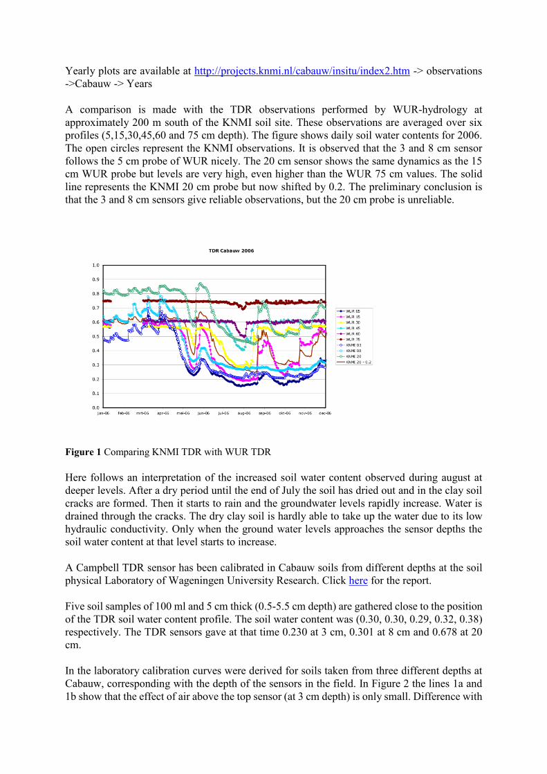
Yearly plots are available at http://projects.knmi.nl/cabauw/insitu/index2.htm -> observations ->Cabauw -> Years

A comparison is made with the TDR observations performed by WUR-hydrology at approximately 200 m south of the KNMI soil site. These observations are averaged over six profiles (5,15,30,45,60 and 75 cm depth). The figure shows daily soil water contents for 2006. The open circles represent the KNMI observations. It is observed that the 3 and 8 cm sensor follows the 5 cm probe of WUR nicely. The 20 cm sensor shows the same dynamics as the 15 cm WUR probe but levels are very high, even higher than the WUR 75 cm values. The solid line represents the KNMI 20 cm probe but now shifted by 0.2. The preliminary conclusion is that the 3 and 8 cm sensors give reliable observations, but the 20 cm probe is unreliable.

Figure 1 Comparing KNMI TDR with WUR TDR

Here follows an interpretation of the increased soil water content observed during august at deeper levels. After a dry period until the end of July the soil has dried out and in the clay soil cracks are formed. Then it starts to rain and the groundwater levels rapidly increase. Water is drained through the cracks. The dry clay soil is hardly able to take up the water due to its low hydraulic conductivity. Only when the ground water levels approaches the sensor depths the soil water content at that level starts to increase.

A Campbell TDR sensor has been calibrated in Cabauw soils from different depths at the soil physical Laboratory of Wageningen University Research. Click here for the report.

Five soil samples of 100 ml and 5 cm thick (0.5-5.5 cm depth) are gathered close to the position of the TDR soil water content profile. The soil water content was (0.30, 0.30, 0.29, 0.32, 0.38) respectively. The TDR sensors gave at that time 0.230 at 3 cm, 0.301 at 8 cm and 0.678 at 20 cm.

In the laboratory calibration curves were derived for soils taken from three different depths at Cabauw, corresponding with the depth of the sensors in the field. In Figure 2 the lines 1a and 1b show that the effect of air above the top sensor (at 3 cm depth) is only small. Difference with

the standard Campbell calibration line (CS EC=1.0 dS/m) is between 0.05 and 0.10 volume fraction. The two deeper layers give approximately the same calibration curve. Deviations with the standard Campbell curve is even larger and range between 0.1 and 0.2. Clay soils have a large electric conductivity and Campbell recommends specific curves for such soils. These curves are also displayed in the figure. The current calibration curves for 8 and 20 cm are about 0.1 below the Campbell curve with the largest EC=3.0 dS/m.

Figure 2 Calibration results and Campbell curves for soils with different Electric Conductivity

The conclusion is that soil specific calibration is important for the Cabauw clay soil type. Also specific calibration for the soil types encountered in the vertical profile is of importance. The calibration curve for the 3 cm level corresponds reasonable with the fabric curve for EC=3.0 dS/ml. The curves for the 8 and 20 cm level are even below this extreme curve. The next step is to implement the soil specific calibration in the dataset (not yet done).

We found a difference between the results of Western and Seyfried (2005) on the one hand and Campbell standard calibration curves and the current Cabauw calibration curves on the other hand. Western and Seyfried found an exponent smaller than 1, whereas Campbell and WUR find an exponent larger than 1 leading to a considerable different relationship. This issue is not yet solved.

20.4 Quality Checks and processing

[TH03MF] [TH08MF] [TH20MF]

Data are archived at the end of the day. This makes up the unvalidated dataset. After each month data are checked for completeness. Data are checked and flagged for mall functioning by visualization of time series. This makes up the validated dataset. Apart from the issues mentioned above no further problems are known for the soil water content observations.

[THL1] [THL2] [THL3] [THL4] [THL5]

[THR1] [THR2] [THR3] [THR4] [THR5]

The sensors produce status codes which are used to judge possible measurement problems. Daily automatic reports signal possible problems in the observations. After each month the data are checked for completeness. Data are checked and flagged for mall functioning by visualization of time series.

21 Ground water level Ground water level at Cabauw is managed. This means that water level in the ditches is regulated to get water out of the polder during wet episodes and into the polder during dry spells, the latter being the exception the first being the rule.

21.1 Parameters

CESAR MB Unit Description Period CESAR dataset MB dataset

GWLSLN GWLSLN m Ground water level r.t. NAP*

Ditch

20000922 - now cesar_soil_water

cabsurf

GWLWNN GWLWNN m Ground water level r.t. NAP*

Meteo-field (soil plot)

20000922 - now cesar_soil_water

cabsurf

GWLWSN GWLWSN m Ground water level r.t. NAP*

Meteo-field (central)

20000922 - now cesar_soil_water

cabsurf

GWLW1N GWLW1N m Ground water level r.t. NAP*

Grass strip (ditch side)

20000922 - now cesar_soil_water

cabsurf

GWLW2N GWLW2N m Ground water level r.t. NAP*

Grass strip (central)

20000922 - now cesar_soil_water

cabsurf

GWLEBN GWLEBN m Ground water level r.t. NAP*

EB-field (soil plot)

20000922 - now cesar_soil_water

cabsurf

GWLWNS GWLWNS m Ground water level r.t. surface

Meteo-field (soil plot)

20000922 - now cesar_soil_water

cabsurf

GWLWSS GWLWSS m Ground water level r.t. surface

Meteo-field (central)

20000922 - now cesar_soil_water

cabsurf

GWLW1S GWLW1S m Ground water level r.t. surface

Grass strip (ditch side)

20000922 - now cesar_soil_water

cabsurf

GWLW2S GWLW2S m Ground water level r.t. surface

Grass strip (central)

20000922 - now cesar_soil_water

Cabsurf

GWLEBS GWLEBS m Ground water level r.t.surface

EB-field (soil plot)

201108009 - now cesar_soil_water

Cabsurf

GWLSL Pa Ground water sensor pressure Ditch 20000922 - now cabsurf

GWLWN Pa Ground water sensor pressure

Meteo-field (soil plot)

20000922 - now

cabsurf

GWLWS Pa Ground water sensor pressure

Meteo-field (central)

20000922 - now

cabsurf

GWLW1 Pa Ground water sensor pressure

Grass strip (ditch side)

20000922 - now

cabsurf

GWLW2 Pa Ground water sensor pressure

Grass strip (central)

20000922 - now

cabsurf

GWLEB Pa Ground water sensor pressure EB-

field (soil plot)

20000922 - now

cabsurf

*Relative to mean sea level (NAP, Normaal Amsterdams Peil)

21.2 Instruments and set-up

[GWLSL] [GWLWN] [WGLWS] [GWLW1] [GWLW2]

(20000922 – now)

Ground water level is measured at 5 positions along an East-West line 100 m South of the main tower. The line crosses a ditch. One of the positions is in the ditch. Pressure sensors (Keller, 26W/8369,0-250mbar) are used to measure the ground water table. Ground water table is measured at 5 locations. A hole of 1.5 m depth and 15 cm diameter is drilled into the ground. A tube with a diameter 48.2 mm is led into the hole and the region between the tube and the hole is filled with small stones. The upper part is filled with the local soil. The tube has holes in the lower part to give access to the ground water. The holes are covered with a fine metal grid to avoid particles entering the measuring region. The sensor is led down into the tube to a well-defined depth. This is defined by the length of a PVC pipe through which the sensor cable is led, with the sensor tight to the lower end of the pipe and the top of the pipe positioned at the cover which is connected to the upper side of the tube.

The sensor in the ditch has a slightly different configuration. Instead of the 15 cm diameter drilled hole there is a 20 cm diameter PVC pipe of uncertain depth (but probably 1.5 m). This PVC pipe is then filled with small stones surrounding the smaller tube. This configuration may lead to delays in adjustment of the water level in the PVC pipe to the actual didge water level outside the PVC pipe.

The instruments are Keller, type 26W/8369,0-250mbar.

(20160830 – 20171030) At the end of this period [GWLSL] was found with the top cap incorrectly positioned. After repositioning an upward change in pressure of 10 mm water equivalent was found. The start of this problem could be traced back. Measurements for this period were corrected.

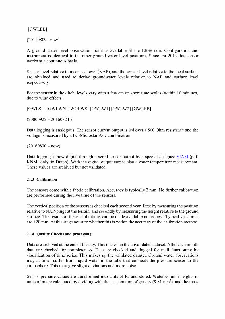
[GWLEB]

(20110809 - now)

A ground water level observation point is available at the EB-terrain. Configuration and instrument is identical to the other ground water level positions. Since apr-2013 this sensor works at a continuous basis.

Sensor level relative to mean sea level (NAP), and the sensor level relative to the local surface are obtained and used to derive groundwater levels relative to NAP and surface level respectively.

For the sensor in the ditch, levels vary with a few cm on short time scales (within 10 minutes) due to wind effects.

[GWLSL] [GWLWN] [WGLWS] [GWLW1] [GWLW2] [GWLEB]

(20000922 – 20160824 )

Data logging is analogous. The sensor current output is led over a 500 Ohm resistance and the voltage is measured by a PC-Microstar A/D combination.

(20160830 – now)

Data logging is now digital through a serial sensor output by a special designed SIAM (pdf, KNMI-only, in Dutch). With the digital output comes also a water temperature measurement. These values are archived but not validated.

21.3 Calibration

The sensors come with a fabric calibration. Accuracy is typically 2 mm. No further calibration are performed during the live time of the sensors.

The vertical position of the sensors is checked each second year. First by measuring the position relative to NAP-plugs at the terrain, and secondly by measuring the height relative to the ground surface. The results of these calibrations can be made available on request. Typical variations are ±20 mm. At this stage not sure whether this is within the accuracy of the calibration method.

21.4 Quality Checks and processing

Data are archived at the end of the day. This makes up the unvalidated dataset. After each month data are checked for completeness. Data are checked and flagged for mall functioning by visualization of time series. This makes up the validated dataset. Ground water observations may at times suffer from liquid water in the tube that connects the pressure sensor to the atmosphere. This may give slight deviations and more noise.

Sensor pressure values are transformed into units of Pa and stored. Water column heights in units of m are calculated by dividing with the acceleration of gravity (9.81 m/s2) and the mass

of 1 m3 of water (1000 kg). Ground water levels relative to NAP and relative to the local surface level are calculated and stored.

21.5 Quicklooks

Yearly graphs of groundwater levels are displayed here (htm, click in table). The graph of the current year is updated each day.

22 Surface geostrophic wind

For the relevant equations relating the pressure field to the geowind see pdf-file.

22.1 Introduction

The geowind appears in the dynamic equaton of the horizontal wind speed as the apparent wind who's Coriolis force would balance the force related to the horizontal pressure gradient. The geowind is one of the important parameters determining the structure of the vertical wind profile. The geowind at a specific location can be derived from accurate pressure observations from nearby weather stations reduced to a horizontal reference frame. By using the data reduced to sea level the surface geowind is derived. At higher levels the geowind is influenced by the thermal wind which is a result of horizontal temperature gradients. Here we limit to surface geowind. Cats (1977, KNMI-WR-77-02) derives geowinds over the Netherlands by means of a principle component analysis of the pressure field over the Netherlands from all the available land surface pressure observations. This method is very efficient for analysing fields. Here we are interested in the geowind at one location, e.g. Cabauw. This can adequately be done by fitting the pressure observations to a polynomial expansion with the x- and y-directional coordinates as arguments. Estimating geowind for one location is a trade of between high resolution in time, by using only nearby stations, and high accuracy by using more and more distant stations.

22.2 Implementation

Figure 6 shows the AWS station over land and sea. In the current observational network data are stored at a rate of 10 minutes (last 1 minute averages) (from december 2002 onward). A longer time series exists of hourly values (synop) where 1-min mean pressure data taken at hh:50 UTC (10 minute to the hour) are archived. Over the time a number of sea locations has been installed which are interesting for the determination of geowind in the Western part of The Netherlands. Reduction to mean sea level is described in " Handboek Waarnemingen" (In Dutch). The method is an approximation of the WMO formulas suitable for the Netherlands were station levels are limited in height. Effects of temperature and humidity on the weight of the air column is accounted for.

We derive various flavours of geowind:

1. From all station with a distance of approximately 50 km or less from Cabauw. This stations are 210, 240, 260, 265, 330, 344, 348, 350. Only linear terms in the representation of the pressure field are used. When all station observations are available the standard deviation in Ugeo = 1.10 m/s and in Vgeo = 0.97 m/s with negligible correlation between the errors in the two components. For the derivation of this standard deviation an accuracy of 0.1 hPa in the pressure observations is assumed. Moreover it is assumed that the linear approximation is not limiting. Both Soesterberg (265) and De Bilt (260) which are relatively close together are incorporated. With a perfect model field this would not be a problem and would increase the accuracy of the estimation. When the linear approximation is not correct this may give too much emphasis on the region around De Bilt-Soesterberg. Observations at station 265 has stopped in 2005.

2. and 3. As 1. but with stations included up to a distance of approximately 100 km from Cabauw. These are 225, 254|554 268|269 275 320 340 370 375. Geostrophic wind estimates are produced both with a linear and a quadratic approximation of the pressurefield. For the linear analysis standard deviation in Ugeo = 0.55 m/s and in Vgeo = 0.43 m/s and negligible correlation between the errors in the two components. Standard deviation in Ugeo = 0.64 m/s and in Vgeo = 0.46 m/s and negligible correlation between the errors in the two components

4.As 3. but with station included up to a distance of 200 km from Cabauw. These are 235 242 250|251 252|550 270 280 290 310|553 380. Because of the larger distances a second order polynomial is used to approximate the pressure field. Standard deviation in Ugeo = 0.28 m/s and in Vgeo = 0.26 m/s and negligible correlation between the errors in the two components.

A number of sea stations has been implemented over the last decade which might be of interest for a more accurate determination of geostrophic wind at Cabauw. Not all these stations has been included yet.

Military airports are in the synop, but until recently not in the AWS database.

For a preliminary account on Lagrangian derivative of the geowind and its interpretation see pdf-file.

Figure 6 (Left panel) AWS stations at land with radii of 50 and 100 km from Cabauw. (Right panel) AWS stations at sea with radii of 100 and 200 km. status 2015)

23 Extra large Aperture Scintillometer (XLAS) Scintillometers make use of a beam of monochromatic electro-magnetic radiation send horizontally through the atmosphere by a transmitter. The beam interacts with refractive index variations in the atmosphere induced by turbulence. This interaction results in fluctuations of the intensity of the beam at the receiver side. The magnitude of the fluctuations can be related to the surface flux of heat and or water vapor. At optical wave lengths the scintillometer is most sensitive to temperature induced density fluctuation.

23.1 XLAS parameters

CESAR MB Unit Description Period CESAR dataset MB dataset

HSCN2 W m-2 CN2 derived sensible heat flux 20020107-20040414

20080110- now

cabsurf

HSCN1 HSCN1 W m-2 CN2 derived sensible heat flux 20020107-20040414

20080110- now

cesar_scintillometer cabsurf

CN2 CN2 degC Structure parameter of

refractive index

20020107-20040414

20080110- now

cesar_scintillometer cabsurf

XLAS XLAS degC XLAS carrier signal 20020107-20040414

20080110- 20170414

cesar_scintillometer cabsurf

XLASD XLASD degC XLAS demodulation signal 20020107-20040414

20080110- now

cesar_scintillometer cabsurf

23.2 Instruments and set-up

An eXtra-Large Aperture Scintillometer is operated over a 9.8 km path from the IJsselstein TV-tower to the Cabauw meteorological tower. The instrument gives the weighted path averaged structure parameter of the refractive index (Cn

2) at the near-infrared wavelength of 0.94 µm. At this wavelength Cn

2 is mainly determined by CT2 the structure parameter of air temperature,

humidity plays a minor but significant role. With Monin-Obukhov similarity CT2 can be related

to the path averaged sensible heat flux. For more information see Kohsiek et al (2002).

[20020107 - 20040414] An XLAS, developed in a cooperation between KNMI and WUR was used at a height of 40 m.

[20080110 – 20151001] The XLAS MkI of Kipp&Zn is operated (manual, pdf). This instrument is based on the earlier versions developed by WUR and KNMI. To avoid the possibility of saturation at high sensible heat fluxes the instrument is now operated with the beam at 60 m height.

[20151002 – 20170414] The XLAS MkI is upgraded to MkII, which includes a better optical focus and a digital data interface (manual, pdf). The same analog data logging is still applied.

[20170131-20170414] Digital data logging is performed in parallel through the EAS. Status codes of the instrument are logged. The meaning of the status codes is given in Appendix E section 2 of the manual. A comparison was made which showed good correspondence between the digital and analogue output of the instrument.

[20170414 – now] Analogue data logging is abandoned

23.3 Calibration

The aperture of the XLAS is of direct importance for the quantitative determination of Cn2 from the scintillometer output signal. It is determined by applying different apertures in front of the receiver and the transmitter. The carrier signal strength should give a quadratic relation with the apertures. The fitted quadratic curve of aperture can be extrapolated to the carrier signal strength received when no aperture is applied.

23.4 Data processing

The instrument gives a demodulation signal (typically -50 mV) and an output signal (V_out, between 0 and -5 V). Both signals are sampled with 2 Hz and treated in a standard way to give 10 minute based statistics. The structure parameter is derived with the following formula:

Cn2 = 10(3.+V_out) in units 10-15 m-2/3

and is applied at sample level. This Cn2 values too are treated in the standard way to get a 10 minute based mean value.

Kohsiek W., W. M. L. Meijninger, A. F. Moene, B.G. Heusinkveld, O.K. Hartogensis, W. C. A. M. Hillen and H. A. R. de Bruin (2002). An extra large aperture scintillometer (XLAS) for long range applications. Boundary Layer Meteorology., 105, 119-127.

A short note (pdf) (still in concept) is under development listing the relevant aspect and formulas to come to a correct interpretation of the XLAS observation.

For interpretation of scintillometer observations at heights well above the surface see:

Braam, M., F.C. Bosveld and A.F. Moene, On MOST scaling in and above the surface layer: the complexities of elevated scintillometer measurements Bound.-Layer Meteorol., 2012, 144, 157-177, doi:10.1007/s10546-012-9716-7.

In short term experiments after 2004 it was found that the XLAS is susceptible for direct sunlight at sun rise (sensor side) and possibly sun set (source side). If possible scintillometer paths are chosen in directions to avoid this possibility, but here we don't have a choice. In the design of the Kipp and Zn instrument care is taken that the sun burning trace through the interior of the instrument just before sunset and just after sunrise cannot damage the wiring. Direct hit of sunlight on the sensor or transmitter can only occur at the moment of sunset and sunrise. At that moments the sunlight intensity seems in all cases be too low to cause damage to the instruments.

23.5 Maintenance

On a regular basis check the desiccant in the drying cartridges. This is a self-indicating silica-gel. When it requires replacement the color changes from orange to clear.

23.6 QA/QC

The received light intensity is monitored. After each month the 10 minute intervals with high visibility are selected and the average of the demodulation signal strength is determined. A decreased value may indicate misalignment of the XLAS system or a degrading light source (see graph).

Each month the XLAS data are visually inspected in a month plot.

24 Bowen ratio from psychrometers

The accuracies of the standard temperature and humidity sensors as described in Section 9 is not sufficient for the accurate estimation of the Bowen ratio. The KNMI psychrometer (Slob, 1978) (KNMI-report, pdf) with double shielding, strong ventilation and temperature measurements based on thermocouples and in-house developed thermocouple amplifiers has been operational at Cabauw until 1996. These sensors have, under favorable conditions an accuracy of a few 0.01 K, which is sufficient for a reliable estimation of the Bowen ratio. The sensors have been redesigned to hold Pt100 elements as temperature sensors and the specially designed SIAM (CAB-P) datalogger (pdf, KNMI-only, in Dutch).

24.1 Psychrometer parameters

CESAR MB Unit Description Period CESAR dataset MB dataset

TD1 oC Dry-bulb temperature at 1 m 20070907- now psychcab

TD2 oC Dry-bulb temperature at 2 m 20070907- now psychcab

TD4 oC Dry-bulb temperature at 4 m 20070907- now psychcab

TW1 oC Wet-bulb temperature at 1 m 20070907- now psychcab

TW2 oC Wet-bulb temperature at 2 m 20070907- now psychcab

TW4 oC Wet-bulb temperature at 4 m 20070907- now psychcab

24.2 Instruments and set-up

(20070907). Three psychrometers are installed in a Bowen ratio configuration at the Energy Balance field. Heights are 1.00, 2.00 and 3.90 m above the surface (see Figure 7). Direction of the psychrometer arms is 257.5 degrees. The ventilation is done with vans placed in the psychrometer arms. Water supply to the wet-bulbs remain problematic. Ventilators are quite often defect. Ventilation speed is around 6 m/s. We have doubts whether this is sufficient to a obtain a good wet-bub temperature. If the wicks are not applied correctly, or if the water supply is to large water bridges may occur as can be seen in Figure 8.

(20170424) Internal ventilators replaced by the good-old Stephan ventilator sucking air through all three psychrometers. Ventilation speed is now much higher, and wet-bulb temperature seems to be more reliable. Also water-bridges are less likely to form as water droplets are blown away.

(20180314) Water supply improved, from now on the measurements are more reliable than before.

(20190507) Ventilator was in the along psychrometer arm direction and outflow was perpendicular to the North. This gives a broad range of wind directions where the psychrometers (specifically the 1 m) may be influenced by the outflow. Ventilator moved to the North of the mast and outflow directed to the North

(20190514) The top sensor height was found to be 388.8 m. The 2 and 4 m height sensors were found to be not level. The 1 m sensor where leveled with help of an inclinometer. The 2 and 4 m sensors by measuring the distances with the 1 m sensors. The ventilator repositioned in the downwind direction of the arms of the psychrometer (approximately NE) and now the outflow also turned into the downwind direction.

Figure 7 Bowen ratio system at Energy Balance terrain with psychrometers at 1, 2 and 4 m above the surface.

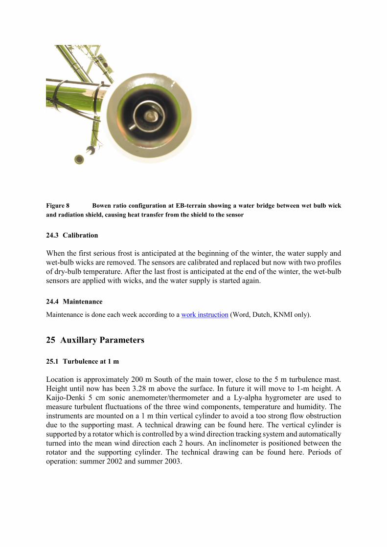
Figure 8 Bowen ratio configuration at EB-terrain showing a water bridge between wet bulb wick and radiation shield, causing heat transfer from the shield to the sensor

24.3 Calibration

When the first serious frost is anticipated at the beginning of the winter, the water supply and wet-bulb wicks are removed. The sensors are calibrated and replaced but now with two profiles of dry-bulb temperature. After the last frost is anticipated at the end of the winter, the wet-bulb sensors are applied with wicks, and the water supply is started again.

24.4 Maintenance

Maintenance is done each week according to a work instruction (Word, Dutch, KNMI only).

25 Auxillary Parameters

25.1 Turbulence at 1 m

Location is approximately 200 m South of the main tower, close to the 5 m turbulence mast. Height until now has been 3.28 m above the surface. In future it will move to 1-m height. A Kaijo-Denki 5 cm sonic anemometer/thermometer and a Ly-alpha hygrometer are used to measure turbulent fluctuations of the three wind components, temperature and humidity. The instruments are mounted on a 1 m thin vertical cylinder to avoid a too strong flow obstruction due to the supporting mast. A technical drawing can be found here. The vertical cylinder is supported by a rotator which is controlled by a wind direction tracking system and automatically turned into the mean wind direction each 2 hours. An inclinometer is positioned between the rotator and the supporting cylinder. The technical drawing can be found here. Periods of operation: summer 2002 and summer 2003.

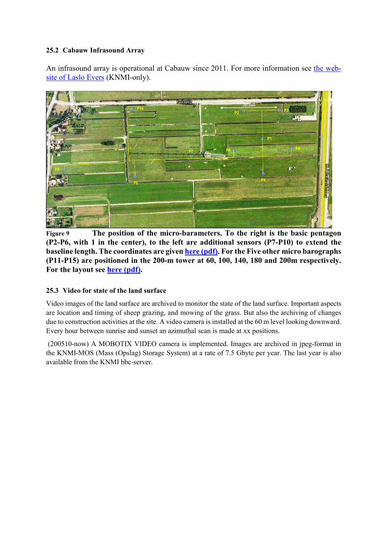
25.2 Cabauw Infrasound Array

An infrasound array is operational at Cabauw since 2011. For more information see the web-site of Laslo Evers (KNMI-only).

Figure 9 The position of the micro-barameters. To the right is the basic pentagon (P2-P6, with 1 in the center), to the left are additional sensors (P7-P10) to extend the baseline length. The coordinates are given here (pdf). For the Five other micro barographs (P11-P15) are positioned in the 200-m tower at 60, 100, 140, 180 and 200m respectively. For the layout see here (pdf).

25.3 Video for state of the land surface

Video images of the land surface are archived to monitor the state of the land surface. Important aspects are location and timing of sheep grazing, and mowing of the grass. But also the archiving of changes due to construction activities at the site. A video camera is installed at the 60 m level looking downward. Every hour between sunrise and sunset an azimuthal scan is made at xx positions.

(200510-now) A MOBOTIX VIDEO camera is implemented. Images are archived in jpeg-format in the KNMI-MOS (Mass (Opslag) Storage System) at a rate of 7.5 Gbyte per year. The last year is also available from the KNMI bbc-server.

26 Regional meteo

Meteorological surface observations of precipitation, cloudfraction, radiation, air pressure, wind speed, wind direction, temperature, relative humidity and visibility from the Automatic Weather station Cabauw and four weather stations surrounding Cabauw are combined into one dataset.

The stations are:

Name WMO number Height Latitude Longitude

Schiphol 6240 -4.4 52.301389 4.774167

De Bilt 6260 2.0 52.100833 5.1775

Zestienhoven 6344 -4.8 51.954722 4.443611

Cabauw 6348 -0.7 51.971667 4.926944

Gilze Rijen 6350 11.1 51.567778 4.933056

26.1 Quality

Maintenance and calibration are are the same as for the Cabauw AWS.

26.2 Origin of the data

Data are derived from the KNMI Climatological Information System. The data are quality checked. Gaps that only occasionally occur are filled.

Royal Netherlands Meteorological Institute

PO Box 201 | NL-3730 AE De BiltNetherlands | WWW.knmi.nl