CA NP 275 1 Q. Evidence of Dr. Vander Weide: When did Dr ...

CA NP 275

Requests for Information NP 2012 COC

Newfoundland Power Inc. – 2012 Cost of Capital Application of 1

Q. Evidence of Dr. Vander Weide: When did Dr. Vander Weide last file evidence on 1

behalf of a U.S. electricity utility in which he provided an estimate of the firm’s cost 2

of equity? Please provide a copy of the evidence filed. 3

4 A. Dr. Vander Weide filed evidence on the cost of equity before the Federal Energy 5

Regulatory Commission (“FERC”) using the FERC’s DCF formula approach on behalf 6

of Mississippi Power Company. The testimony is attached. 7

CA NP 275

Attachment A

Requests for Information NP 2012 COC

Newfoundland Power Inc. – 2012 Cost of Capital Application

Federal Energy Regulatory Commission

Docket No. ER012-___-000

Testimony of Dr. James H. Vander Weide

UNITED STATES OF AMERICA

BEFORE THE

FEDERAL ENERGY REGULATORY COMMISSION

MISSISSIPPI POWER COMPANY / DOCKET NO. ER012-___-000

MISSISSIPPI POWER COMPANY

PREPARED DIRECT TESTIMONY OF DR. JAMES H. VANDER WEIDE

NOVEMBER 2011

i

MISSISSIPPI POWER COMPANY RATE OF RETURN

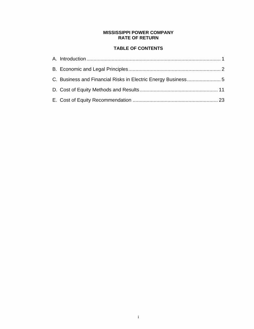
TABLE OF CONTENTS

A. Introduction ................................................................................................ 1

B. Economic and Legal Principles.................................................................. 2

C. Business and Financial Risks in Electric Energy Business ........................ 5

D. Cost of Equity Methods and Results........................................................ 11

E. Cost of Equity Recommendation ............................................................. 23

MISSISSIPPI POWER COMPANY RATE OF RETURN

LIST OF EXHIBITS AND APPENDICES

ii

Schedule 1 Summary of Discounted Cash Flow Analysis Group I-Large

Proxy Electric Company Group Using the Commission’s

Methodology in 92 FERC ¶ 61,070 (2000)

Schedule 2 Summary of Discounted Cash Flow Analysis Group II-Electric

Company Group with BBB+ or Higher Bond Ratings Using the

Commission’s Methodology in 92 FERC ¶ 61,070 (2000)

Schedule 3 Summary of Discounted Cash Flow Analysis for Large Proxy

Electric Company Group Using a Quarterly DCF Model

Appendix 1 Appendix 1 Derivation of the Quarterly DCF Model

Appendix 2 Appendix 2 Adjusting for Flotation Costs in Determining a Public

Utility’s Allowed Rate of Return on Equity

Appendix 3 Statement of Qualifications

Attachment 1 Summary of Professional Experience

UNITED STATES OF AMERICA 1 BEFORE THE 2

FEDERAL ENERGY REGULATORY COMMISSION 3

MISSISSIPPI POWER COMPANY DOCKET NO. ER012-___-000 4

PREPARED DIRECT TESTIMONY OF JAMES H. VANDER WEIDE 5 ON BEHALF OF 6

MISSISSIPPI POWER COMPANY 7

A. Introduction 8

Q. 1 Please state your name, title, and business address for the record. 9

A. 1 My name is James H. Vander Weide. I am Research Professor of 10

Finance and Economics at Duke University, the Fuqua School of 11

Business. I am also President of Financial Strategy Associates, a firm 12

that provides strategic and financial consulting services to corporate 13

clients. My business address is 3606 Stoneybrook Drive, Durham, North 14

Carolina 27705. 15

Q. 2 Please describe your educational background and prior academic 16

experience. 17

A. 2 I graduated from Cornell University with a Bachelor's Degree in 18

Economics and from Northwestern University with a Ph.D. in Finance. 19

After joining the faculty of the School of Business at Duke University, I 20

was named Assistant Professor, Associate Professor, Professor, and 21

then Research Professor. I have published research in the areas of 22

finance and economics and taught courses in these fields at Duke for 23

more than thirty-five years. I am now retired from my teaching duties at 24

Duke. A summary of my research, teaching, and other professional 25

experience is presented in Attachment 1. 26

Q. 3 Have you previously testified on financial or economic issues? 27

A. 3 Yes. As an expert on financial and economic theory and practice, I have 28

participated in more than 400 regulatory and legal proceedings before 29

the U.S. Congress, the Canadian Radio-Television and 30

Telecommunications Commission, the Federal Communications 31

Commission, the National Telecommunications and Information 32

Administration, the Federal Energy Regulatory Commission, the National 33

Energy Board (Canada), the public service commissions of forty-three 34

states and three Canadian provinces, the insurance commissions of five 1

states, the Iowa State Board of Tax Review, the National Association of 2

Securities Dealers, and the North Carolina Property Tax Commission. In 3

addition, I have prepared expert testimony in proceedings before the 4

U.S. Tax Court, the U.S. District Court for the District of Nebraska; the 5

U.S. District Court for the District of New Hampshire; the U.S. District 6

Court for the District of Northern Illinois; the U.S. District Court for the 7

Eastern District of North Carolina; the Montana Second Judicial District 8

Court, Silver Bow County; the U.S. District Court for the Northern District 9

of California; the Superior Court, North Carolina; the U.S. Bankruptcy 10

Court for the Southern District of West Virginia; and the U. S. District 11

Court for the Eastern District of Michigan. 12

Q. 4 What is the purpose of your testimony? 13

A. 4 I have been asked by Mississippi Power Company (“Mississippi Power” 14

or “the Company”) to prepare an independent appraisal of Mississippi 15

Power’s cost of equity and to recommend a rate of return on equity 16

(“ROE”) that is fair, that allows Mississippi Power to attract capital on 17

reasonable terms, and that allows Mississippi Power to maintain its 18

financial integrity. 19

B. Economic and Legal Principles 20

Q. 5 How do economists define the required rate of return, or cost of capital, 21

associated with particular investment decisions, such as the decision to 22

invest in electric generation, transmission, and distribution facilities? 23

A. 5 Economists define the cost of capital as the return investors expect to 24

receive on alternative investments of comparable risk. 25

Q. 6 How does the cost of capital affect a firm’s investment decisions? 26

A. 6 The goal of a firm is to maximize the value of the firm. This goal can be 27

accomplished by accepting all investments in plant and equipment with 28

an expected rate of return greater than the cost of capital. Thus, a firm 29

should continue to invest in plant and equipment only so long as the 30

return on its investment is greater than or equal to its cost of capital. 31

Q. 7 How does the cost of capital affect investors’ willingness to invest in a 32

company? 33

A. 7 The cost of capital measures the return investors can expect on 1

investments of comparable risk. The cost of capital also measures the 2

investor’s required rate of return on investment because rational 3

investors will not invest in a particular investment opportunity if the 4

expected return on that opportunity is less than the cost of capital. Thus, 5

the cost of capital is a hurdle rate for both investors and the firm. 6

Q. 8 Do all investors have the same position in the firm? 7

A. 8 No. Debt investors have a fixed claim on a firm’s assets and income that 8

must be paid prior to any payment to the firm’s equity investors. Since 9

the firm’s equity investors have a residual claim on the firm’s assets and 10

income, equity investments are riskier than debt investments. Thus, the 11

cost of equity exceeds the cost of debt. 12

Q . 9 What is the overall or average cost of capital? 13

A. 9 The overall or average cost of capital is a weighted average of the cost 14

of debt and cost of equity, where the weights are the percentages of debt 15

and equity in a firm’s capital structure. 16

Q. 10 Can you illustrate the calculation of the overall or weighted average cost 17

of capital? 18

A. 10 Yes. Assume that the cost of debt is 7 percent, the cost of equity is 19

13 percent, and the percentages of debt and equity in the firm’s capital 20

structure are 50 percent and 50 percent, respectively. Then the 21

weighted average cost of capital is expressed by .50 times 7 percent 22

plus .50 times 13 percent, or 10.0 percent. 23

Q. 11 How do economists define the cost of equity? 24

A. 11 Economists define the cost of equity as the return investors expect to 25

receive on alternative equity investments of comparable risk. Since the 26

return on an equity investment of comparable risk is not a contractual 27

return, the cost of equity is more difficult to measure than the cost of 28

debt. However, as I have already noted, there is agreement among 29

economists that the cost of equity is greater than the cost of debt. There 30

is also agreement among economists that the cost of equity, like the cost 31

of debt, is both forward looking and market based. 32

Q. 12 Does the required rate of return on an investment vary with the risk of 33

that investment? 34

A. 12 Yes. Since investors are averse to risk, they require a higher rate of 1

return on investments with greater risk. 2

Q. 13 Do economists and investors consider future industry changes when 3

they estimate the risk of a particular investment? 4

A. 13 Yes. Economists and investors consider all the risks that a firm might 5

incur over the future life of the company. 6

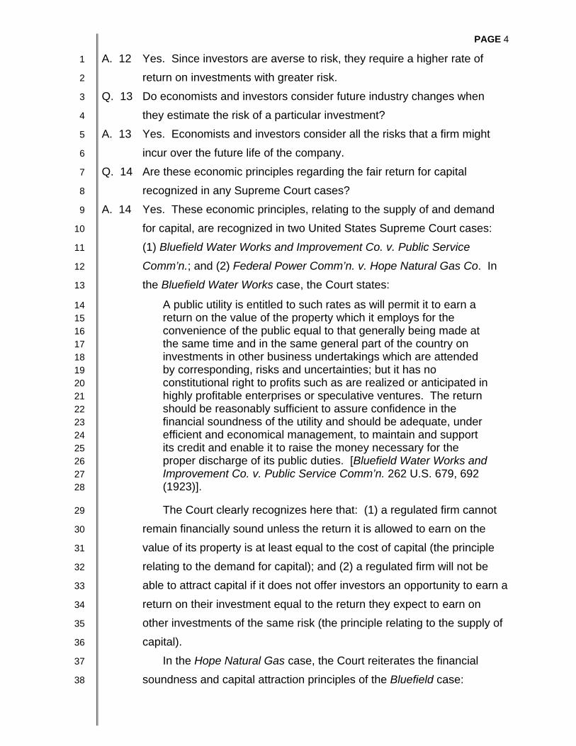
Q. 14 Are these economic principles regarding the fair return for capital 7

recognized in any Supreme Court cases? 8

A. 14 Yes. These economic principles, relating to the supply of and demand 9

for capital, are recognized in two United States Supreme Court cases: 10

(1) Bluefield Water Works and Improvement Co. v. Public Service 11

Comm’n.; and (2) Federal Power Comm’n. v. Hope Natural Gas Co. In 12

the Bluefield Water Works case, the Court states: 13

A public utility is entitled to such rates as will permit it to earn a 14 return on the value of the property which it employs for the 15 convenience of the public equal to that generally being made at 16 the same time and in the same general part of the country on 17 investments in other business undertakings which are attended 18 by corresponding, risks and uncertainties; but it has no 19 constitutional right to profits such as are realized or anticipated in 20 highly profitable enterprises or speculative ventures. The return 21 should be reasonably sufficient to assure confidence in the 22 financial soundness of the utility and should be adequate, under 23 efficient and economical management, to maintain and support 24 its credit and enable it to raise the money necessary for the 25 proper discharge of its public duties. [Bluefield Water Works and 26 Improvement Co. v. Public Service Comm’n. 262 U.S. 679, 692 27 (1923)]. 28

The Court clearly recognizes here that: (1) a regulated firm cannot 29

remain financially sound unless the return it is allowed to earn on the 30

value of its property is at least equal to the cost of capital (the principle 31

relating to the demand for capital); and (2) a regulated firm will not be 32

able to attract capital if it does not offer investors an opportunity to earn a 33

return on their investment equal to the return they expect to earn on 34

other investments of the same risk (the principle relating to the supply of 35

capital). 36

In the Hope Natural Gas case, the Court reiterates the financial 37

soundness and capital attraction principles of the Bluefield case: 38

From the investor or company point of view it is important that 1 there be enough revenue not only for operating expenses but 2 also for the capital costs of the business. These include service 3 on the debt and dividends on the stock [citation omitted]. By that 4 standard the return to the equity owner should be commensurate 5 with returns on investments in other enterprises having 6 corresponding risks. That return, moreover, should be sufficient 7 to assure confidence in the financial integrity of the enterprise, so 8 as to maintain its credit and to attract capital. [Federal Power 9 Comm’n. v. Hope Natural Gas Co., 320 U.S. 591, 603 (1944)]. 10

C. Business and Financial Risks in Electric Energy Business 11

Q. 15 What are the primary factors that affect the business and financial risks 12

of electric energy companies such as Mississippi Power? 13

A. 15 The business and financial risks of electric energy companies such as 14

Mississippi Power are affected by a number of economic factors, 15

including: 16

1. Demand Uncertainty. Demand uncertainty is one of the primary 17

business risks of investing in electric energy companies such as 18

Mississippi Power. Demand uncertainty is caused by: (a) the strong 19

dependence of electric demand on the state of the economy and 20

weather patterns; (b) the ability of customers to choose alternative 21

forms of energy, such as natural gas or oil; (c) the ability of some 22

customers to locate facilities in the service areas of competitors; 23

(d) the ability of some customers to conserve energy or produce their 24

own electricity under cogeneration or self-generation arrangements; 25

and (e) the ability of municipalities to go into the energy business 26

rather than renew the company’s franchise. Demand uncertainty is a 27

problem for electric companies because of the need to plan for 28

infrastructure additions many years in advance of demand. 29

2. Operating Uncertainty. The business risk of electric energy 30

companies is also increased by the inherent uncertainty in the typical 31

electric energy company’s operations. Operating uncertainty arises 32

as a result of: (a) high volatility in fuel prices or interruptions in fuel 33

supply; (b) the prospect of rising employee health care and pension 34

expenses; (c) uncertainty over plant outages, the cost of purchased 35

power, and the revenues achieved from off system sales; 36

(d) variability in maintenance costs and the costs of other materials, 37

(e) uncertainty over outages of the transmission and distribution 1

systems, as well as storm-related expenses; and (f) the prospect of 2

increased expenses for security. 3

3. Investment Uncertainty. The electric energy business requires very 4

large investments in the generation, transmission, and distribution 5

facilities required to deliver energy to customers. The future 6

amounts of required investments in these facilities are highly 7

uncertain as a result of: (a) demand uncertainty; (b) the prospect 8

that Congress or state legislatures will pass stricter environmental 9

regulations and clean air requirements; (c) the prospect of needing to 10

incur additional investments to insure the reliability of the company’s 11

transmission and distribution networks; (d) uncertainty regarding the 12

regulatory and management structure of the electric transmission 13

network; and (e) uncertainty regarding future decommissioning 14

costs. Furthermore, the risk of investing in electric energy facilities is 15

increased by the irreversible nature of the company’s investments in 16

generation, transmission, and distribution facilities. For example, if 17

an electric energy company decides to make a major capital 18

expenditure in a generation plant, and, as a result of new 19

environmental regulations, energy produced by the plant becomes 20

uneconomic, the company may not be able to recover its investment. 21

4. High Operating Leverage. The electric energy business requires a 22

large commitment to fixed costs in relation to the operating margin 23

on sales, a situation known as high operating leverage. The 24

relatively high degree of fixed costs in the electric energy business 25

arises from the average electric energy company’s large investment 26

in fixed generation, transmission, and distribution facilities. High 27

operating leverage causes the average electric energy company’s 28

operating income to be highly sensitive to revenue fluctuations. 29

5. High Degree of Financial Leverage. The large capital requirements 30

for building economically efficient electric generation, transmission, 31

and distribution facilities, along with the traditional regulatory 32

preference for the use of debt, have encouraged electric utilities to 33

maintain highly debt-leveraged capital structures as compared to 34

non-utility firms. High debt leverage is a source of additional risk to 1

utility stock investors because it increases the percentage of the 2

firm’s costs that are fixed. The use of financial leverage also 3

reduces the firm’s interest coverage and increases vulnerability to 4

variations in earnings. 5

6. Regulatory Uncertainty. Investors’ perceptions of the business and 6

financial risks of electric energy companies are strongly influenced 7

by their views of the quality of regulation. Investors are painfully 8

aware that regulators in some jurisdictions have been unwilling at 9

times to set rates that allow companies an opportunity to recover 10

their cost of service and earn a fair and reasonable return on 11

investment. As a result of the perceived increase in regulatory risk, 12

investors will demand a higher rate of return for electric energy 13

companies operating in those states. On the other hand, if investors 14

perceive that regulators will provide a reasonable opportunity for the 15

company to maintain its financial integrity and earn a fair rate of 16

return on its investment, investors will view regulatory risk as 17

minimal. 18

Q. 16 Have any of these risk factors changed in recent years? 19

A. 16 Yes. The risk of investing in electric energy companies has increased as 20

a result of significantly greater macroeconomic uncertainty; higher 21

projected electric energy company capital expenditures; greater volatility 22

in fuel prices; greater uncertainty in the cost of satisfying environmental 23

requirements; more volatile purchased power and off system sales 24

prices; greater uncertainty in employee health care and pension 25

expenses; greater uncertainty with regard to legislative mandates related 26

to generation mix, such as renewable portfolio standards; and greater 27

uncertainty in the expenses associated with system outages, storm 28

damage, and security. Each of these factors puts pressure on customer 29

rates and therefore increases regulatory risk. 30

Q. 17 How does greater macroeconomic uncertainty affect the business and 31

financial risks of investing in electric energy companies such as 32

Mississippi Power? 33

A. 17 Greater macroeconomic uncertainty increases the business and financial 1

risks of investing in electric energy companies such as Mississippi Power 2

by fundamentally increasing demand uncertainty, investment uncertainty, 3

and regulatory uncertainty. 4

Q. 18 Why does macroeconomic uncertainty increase demand uncertainty? 5

A. 18 Macroeconomic uncertainty increases demand uncertainty because the 6

demand for electric energy services depends on the state of the 7

economy. The greater the uncertainty regarding the state of the 8

economy, the greater will be the uncertainty regarding the demand for 9

energy. 10

Q. 19 How does increased demand uncertainty affect the uncertainty of the 11

future return on investment for Mississippi Power? 12

A. 19 Increased demand uncertainty greatly increases the uncertainty of the 13

future return on investment for Mississippi Power because most of the 14

Company’s costs are fixed, while its revenues are variable. Thus, 15

greater volatility in revenues produces greater volatility in return on 16

investment. 17

Q. 20 Why does macroeconomic uncertainty increase investment cost 18

uncertainty? 19

A. 20 Increased macroeconomic uncertainty greatly increases the uncertainty 20

of investment costs for electric companies like Mississippi Power 21

because it increases the uncertainty regarding: the demand for electric 22

energy; the economics of alternative generating technologies; the cost of 23

environmental regulations; the cost of construction materials and labor; 24

and the amount of additional investment required to ensure the reliability 25

of the company’s transmission and distribution networks. 26

Q. 21 Why does macroeconomic uncertainty increase regulatory uncertainty? 27

A. 21 Regulatory uncertainty arises because investors are not certain that 28

regulators will be willing to set rates that allow companies an opportunity 29

to recover their costs of service and earn a fair and reasonable return on 30

investment. Regulatory uncertainty increases in difficult economic times 31

because investors recognize that regulators are likely to face greater 32

pressure to restrain rate increases in difficult economic times than in 33

good economic times. 34

Q. 22 How do greater projected capital expenditures affect the business risks 1

of investing in electric energy companies such as Mississippi Power? 2

A. 22 Greater projected capital expenditures increase the business risks of 3

investing in electric energy companies such as Mississippi Power by 4

increasing investment cost uncertainty, operating leverage, and 5

regulatory uncertainty. 6

Q. 23 Why do greater projected capital expenditures increase an electric 7

energy company’s investment cost uncertainty? 8

A. 23 Greater projected capital expenditures increase investment cost 9

uncertainty because investments in new generation, transmission, and 10

distribution facilities take many years to complete. As investors found 11

during the last electric energy investment boom of the 1980s, actual 12

costs of building new generation, transmission, and distribution facilities 13

can differ from forecasted costs as a result of changes in environmental 14

regulations, materials costs, capital costs, and unexpected delays. 15

Q. 24 Why do greater projected capital expenditures increase operating 16

leverage? 17

A. 24 As noted above, operating leverage increases when a firm’s commitment 18

to fixed costs rises in relation to its operating margin on sales. Increased 19

capital expenditures increase operating leverage because investment 20

costs are fixed, the investment period is long, and revenues do not 21

generally increase in line with investment costs until the investment is 22

entirely included in rate base. Thus, the ratio of fixed costs to operating 23

margin increases when capital expenditures increase. 24

Q. 25 Why do greater projected capital expenditures increase regulatory 25

uncertainty? 26

A. 25 As noted above, regulatory uncertainty arises because investors are 27

aware that regulators in some states have been unwilling at times to set 28

rates that allow a company an opportunity to recover its cost of service, 29

including the cost of capital. Regulatory uncertainty is most pronounced 30

when rates are projected to increase. Greater projected capital 31

expenditures increase regulatory uncertainty because they frequently 32

cause rates to increase. 33

Q. 26 How do greater projected capital expenditures affect the financial risk of 1

investing in electric energy companies? 2

A. 26 The effect of greater projected capital expenditures on the financial risk 3

of investing in electric energy companies depends on the regulatory 4

treatment of Construction Work in Progress (“CWIP”). Greater capital 5

expenditures generally increase financial risk because the plant and 6

equipment associated with the capital expenditures are not included in 7

rate base until the project is complete. However, the impact of higher 8

capital expenditures on financial risk is reduced if CWIP is included in 9

rate base. 10

Q. 27 Is the Company projecting significant capital expenditures over the next 11

several years? 12

A. 27 The Company is projecting capital expenditures of $818 million in 2011, 13

$1 billion in 2012, and $878 million in 2013. Most of these construction 14

expenditures are associated with Mississippi Power’s investment in the 15

Kemper Integrated Gasification Combined Cycle (“IGCC”) generation 16

plant, which has been approved by the Mississippi Public Service 17

Commission. In contrast to these projected capital expenditures, the 18

Company’s capital expenditures were approximately $102 million in 2009 19

and $247 million in 2010.[1] 20

Q. 28 Why are investments in new generation facilities especially risky? 21

A. 28 Investment in new generation facilities is especially risky because the 22

required investment is large, illiquid, and irreversible; the investment 23

horizon is unusually long; the investment and operating costs are highly 24

uncertain; and environmental and safety regulations may change 25

significantly over the life of the investment. In addition, there is no 26

consensus on the best generation option for all utilities. The natural gas 27

option has a lower investment cost and shorter investment horizon, but 28

fuel costs are highly volatile. The coal and nuclear options have 29

significantly lower long-run expected operating costs, but a higher 30

required investment and a longer investment horizon. Renewable 31

energy, though desirable from an environmental standpoint, may be 32

[1] See Mississippi Power Company, 2010 Form 10-K, p. II - 360.

more expensive than other alternatives and may not produce reliable 1

energy in peak periods. The uncertainties associated with all generation 2

options create additional risks for electric utilities. 3

Q. 29 Can the risks facing Mississippi Power and other electric energy 4

companies be distinguished from the risks of investing in companies in 5

other industries? 6

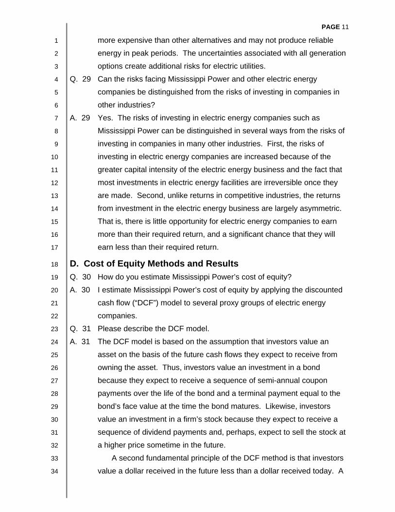
A. 29 Yes. The risks of investing in electric energy companies such as 7

Mississippi Power can be distinguished in several ways from the risks of 8

investing in companies in many other industries. First, the risks of 9

investing in electric energy companies are increased because of the 10

greater capital intensity of the electric energy business and the fact that 11

most investments in electric energy facilities are irreversible once they 12

are made. Second, unlike returns in competitive industries, the returns 13

from investment in the electric energy business are largely asymmetric. 14

That is, there is little opportunity for electric energy companies to earn 15

more than their required return, and a significant chance that they will 16

earn less than their required return. 17

D. Cost of Equity Methods and Results 18

Q. 30 How do you estimate Mississippi Power’s cost of equity? 19

A. 30 I estimate Mississippi Power’s cost of equity by applying the discounted 20

cash flow (“DCF”) model to several proxy groups of electric energy 21

companies. 22

Q. 31 Please describe the DCF model. 23

A. 31 The DCF model is based on the assumption that investors value an 24

asset on the basis of the future cash flows they expect to receive from 25

owning the asset. Thus, investors value an investment in a bond 26

because they expect to receive a sequence of semi-annual coupon 27

payments over the life of the bond and a terminal payment equal to the 28

bond’s face value at the time the bond matures. Likewise, investors 29

value an investment in a firm’s stock because they expect to receive a 30

sequence of dividend payments and, perhaps, expect to sell the stock at 31

a higher price sometime in the future. 32

A second fundamental principle of the DCF method is that investors 33

value a dollar received in the future less than a dollar received today. A 34

future dollar is valued less than a current dollar because investors could 1

invest a current dollar in an interest earning account and increase their 2

wealth. This principle is called the time value of money. 3

Applying the two fundamental DCF principles noted above to an 4

investment in a bond leads to the conclusion that investors value their 5

investment in the bond on the basis of the present value of the bond’s 6

future cash flows. Thus, the price of the bond should be equal to: 7

EQUATION 1 8

where: 9

PB = Bond price; 10

C = Cash value of the coupon payment (assumed for 11

notational convenience to occur annually rather than 12

semi-annually); 13

F = Face value of the bond; 14

i = The rate of interest the investor could earn by investing 15

his money in an alternative bond of equal risk; and 16

n = The number of periods before the bond matures. 17

Applying these same principles to an investment in a firm’s stock 18

suggests that the price of the stock should be equal to: 19

EQUATION 2 20

where: 21

PS = Current price of the firm’s stock; 22

D1, D2...Dn = Expected annual dividend per share on the firm’s stock; 23

Pn = Price per share of stock at the time the investor expects 24

to sell the stock; and 25

k = Return the investor expects to earn on alternative 1

investments of the same risk, i.e., the investor’s required 2

rate of return. 3

Equation (2) is frequently called the annual discounted cash flow 4

model of stock valuation. Assuming that dividends grow at a constant 5

annual rate, g, this equation can be solved for k, the cost of equity. The 6

resulting cost of equity equation is k = D1/Ps + g, where k is the cost of 7

equity, D1 is the expected next period annual dividend, Ps is the current 8

price of the stock, and g is the constant annual growth rate in earnings, 9

dividends, and book value per share. The term D1/Ps is called the 10

dividend yield component of the annual DCF model, and the term g is 11

called the growth component of the annual DCF model. 12

Q. 32 Has the Commission made any decision on the DCF methodology that is 13

applicable to electric companies? 14

A. 32 Yes. The Commission described such a DCF methodology in its 2000 15

SCE decision, subsequently affirmed in the Midwest ISO, New England 16

ISO, and other orders.[2] 17

Q. 33 How does the Commission estimate the dividend yield component of the 18

DCF model in that case? 19

A. 33 The Commission estimates the average low and high dividend yield for 20

each month in a six-month period. It then adjusts the low and high 21

dividend yields for one-half year of growth. 22

Q. 34 How does the Commission estimate the growth component of the DCF 23

model in that case? 24

A. 34 The Commission estimates the growth component of the DCF model in 25

two ways. First, it uses the familiar Gordon equation, br + sv, where br is 26

internal growth and sv is growth from external financing. Second, the 27

Commission uses the I/B/E/S mean estimate of long-term growth for 28

each company. 29

Q. 35 Do you apply the Commission’s DCF method from the SCE case? 30

[2] See, for example, Southern California Edison Co., 92 FERC¶ 61,070

(2000) (“SCE”); Midwest Independent Transmission System Operator, Inc., 100 FERC ¶ 61,292 (2002) (“Midwest ISO”); Bangor Hydro-Electric Co., 117 FERC¶ 61,129 (2006) (“New England ISO”).

A. 35 Yes. I apply the Commission’s DCF methodology to two groups of proxy 1

electric companies. Group I consists of Value Line electric utilities that: 2

(1) paid dividends during every quarter and did not decrease dividends 3

during the last two years; (2) have at least two analysts included in the 4

I/B/E/S mean growth forecast; (3) have a Value Line Safety Rank of 1, 2, 5

or 3; (4) have an investment grade bond rating; and (5) are not the 6

subject of a merger offer that has not been completed. Group II consists 7

of electric utilities that satisfy the same criteria as Group I, but also have 8

Standard & Poor’s bond ratings in the range BBB+ or higher. 9

Q. 36 Group I contains twenty-nine electric utilities. Are there any benefits 10

from including a large group of electric utilities in a proxy group for the 11

purpose of estimating the cost of equity? 12

A. 36 Yes. The DCF model requires inputs of quantities such as investors’ 13

growth expectations that are inherently uncertain because they relate to 14

the future rather than the past. Since investors’ growth expectations are 15

inherently uncertain, there is also some degree of uncertainty 16

surrounding the estimate of the cost of equity for each company. 17

However, the uncertainty in the estimate of the cost of equity for an 18

individual company can be greatly reduced by applying the DCF model 19

to a reasonably large sample of comparable companies. Intuitively, 20

unusually high estimates for some individual companies are offset by 21

unusually low estimates for other individual companies. Thus, financial 22

economists invariably apply cost of equity methodologies to a group of 23

comparable companies. In utility regulation, the practice of using a 24

group of comparable companies is further supported by the regulatory 25

standard that the utility should be allowed to earn a return on its 26

investment that is commensurate with returns being earned on other 27

investments of the same risk.[3] 28

Q. 37 In your second proxy group, Group II, why do you include only those 29

companies with bond ratings of BBB+ or higher? 30

[3] See Bluefield Water Works and Improvement Co. v. Public Service

Comm’n., 262 U.S. 679, 692 (1923) and Federal Power Comm’n v. Hope Natural Gas Co., 320 U.S. 591, 603 (1944).

A. 37 I include only those companies with bond ratings of BBB+ or higher in 1

Group II because Mississippi Power’s bond rating is A, and some 2

analysts might consider companies with bond ratings in the BBB+ or 3

higher range to be similar in risk to Mississippi Power. 4

Q. 38 Did the Commission use a range of bond ratings to select proxy 5

companies in its SCE Decision? 6

A. 38 Yes. The Commission selected companies with bond ratings in the 7

range A+ to A- at a time when SCE’s bond rating was A. 8

Q. 39 Has the Commission changed its criteria for selecting proxy companies 9

in recent decisions? 10

A. 39 Yes. The Commission seems to have changed its preferred criteria for 11

selecting proxy companies in the Midwest ISO, New England ISO, and 12

Atlantic Path Orders[4]. In these orders, the Commission selects proxy 13

groups composed of electric energy companies that operate in the same 14

region of the country as the entity whose rates are being set. 15

Q. 40 Does financial and economic theory require that proxy companies 16

operate in the same region of the country as the company (the target 17

company) whose cost of equity is being estimated? 18

A. 40 No. Financial economists define the cost of equity as the return 19

investors expect to earn on other investments of the same or comparable 20

risk. As long as the proxy group has approximately the same risk on 21

average as the target company, the geographic region in which the proxy 22

companies operate is irrelevant to cost of equity estimation. This 23

conclusion is especially true in a world where capital flows freely across 24

geographic boundaries. 25

Q. 41 Are there any problems with limiting the set of proxy companies only to 26

those companies that operate in the same geographic region as the 27

target company? 28

A. 41 Yes. First, the companies that operate in the same geographic region as 29

the target company may not be comparable in risk to the target 30

[4] See, for example, Midwest ISO; New England ISO; and Atlantic Path 15,

LLC, 122 FERC ¶ 61,135 (2008) (“Atlantic Path”).

company. In such a case, the average cost of equity for the proxy 1

companies will not equal the target company’s cost of equity. 2

Second, restricting the proxy group only to companies that operate in 3

the same geographic region unnecessarily limits the number of 4

companies in the sample group. As discussed above, the uncertainty in 5

the estimate of the cost of equity for an individual company can be 6

significantly reduced by applying cost of equity methodologies to a 7

reasonably large sample of comparable companies rather than to a 8

smaller group that operates in the same geographic region as the target 9

company. 10

Third, the choice of boundaries for the geographic region in which 11

the target company operates can be subjective. When the analyst 12

applies judgment to select a geographic region for the proxy company 13

group, the analyst may be tempted to choose a region that includes 14

proxy companies that produce a desired result. The analyst can 15

eliminate the possibility of selection bias by starting with the largest 16

possible group of comparable risk companies and eliminating only those 17

companies with insufficient data to estimate the cost of equity. 18

Fourth, the use of geographic region as a criteria for selecting proxy 19

companies could result in different estimates of the cost of equity for 20

comparable risk companies with operations in different regions of the 21

country. Such an outcome would produce incorrect economic signals for 22

investment decisions. 23

Q. 42 What results do you obtain from your application of the Commission’s 24

DCF model to the electric utilities in Groups I and II? 25

A. 42 For both Group I and Group II, I obtain midpoint DCF results of 26

11.1 percent, median results of 9.6 percent, and average results of 27

9.6 percent (see Schedule 1 and Schedule 2). The average of the 28

midpoint, median, and mean results is 10.1 percent. This average result 29

excludes low DCF results that are less than one hundred basis points 30

above the six-month average 2011 yield on bonds with the same rating 31

as the company, and excludes high DCF results that exceed 1

17.7 percent.[5] 2

Q. 43 How does the Commission arrive at its cost of equity in the SCE Order? 3

A. 43 The Commission arrives at its cost of equity by calculating the midpoint 4

of the range of DCF results for each company in the proxy group. 5

Q. 44 Has the Commission continued to base the cost of equity on the midpoint 6

of DCF results in recent decisions? 7

A. 44 No. In recent decisions, the Commission has based the approved cost 8

of equity on the median rather than the midpoint of the proxy group DCF 9

results.[6] 10

Q. 45 Do you agree with the Commission’s use of the median DCF result of its 11

chosen proxy group to set the allowed return on equity? 12

A. 45 No. However, I respectfully disagree with the Commission’s use of the 13

median DCF result because the median result is generally an unreliable 14

estimate of a company’s cost of equity. 15

Q. 46 Can you explain why the median DCF result for a proxy group of 16

companies is likely to be an unreliable indicator of the cost of equity? 17

A. 46 Yes. The median result is likely to be an unreliable indicator of the cost 18

of equity because it considers only the rank order of the results and not 19

the values of any results other than those of the one or two middle 20

companies. 21

Q. 47 Have you also estimated Mississippi Power’s cost of equity using an 22

alternative DCF methodology? 23

A. 47 Yes. 24

Q. 48 How does your alternative DCF methodology differ from the 25

Commission’s methodology described in the SCE case? 26

[5] See, for example, SCE and New England ISO. In SCE, the Commission

excludes a return that is insufficiently above the cost of debt, stating: “Because investors generally cannot be expected to purchase stock if debt, which has less risk than stock, yields essentially the same return, this low end-return cannot be considered reliable in this case.” 92 FERC at ¶ 61,266. In New England ISO, the Commission excludes a high result of 17.7 percent. See 117 FERC at ¶¶ 8 and 16.

[6] See, for example, Golden Spread Electric Cooperative, Inc. 123 FERC ¶ 61,047 (2008) (“Golden Spread”).

A. 48 My approach differs from that employed by the Commission in several 1

ways. First, I recommend using a quarterly DCF model rather than an 2

annual DCF model. Second, I rely on the I/B/E/S analysts’ earnings 3

growth estimates as the estimate of growth in the DCF model, rather 4

than on a combination of I/B/E/S and the “br + sv” growth used by the 5

Commission. Third, I recommend the use of the average of the high and 6

low stock prices for the most recent three-month period rather than the 7

most recent six-month period. Fourth, I recommend including an 8

allowance for flotation costs. 9

Q. 49 Please explain why you recommend use of a quarterly DCF model. 10

A. 49 I recommend the use of a quarterly DCF model because it is the only 11

model that produces correct estimates of a firm’s cost of equity capital if 12

the firm pays quarterly dividends, whereas the annual DCF model of 13

stock valuation produces correct estimates of a firm’s cost of equity 14

capital if the firm pays dividends only once a year. Since most U.S. 15

industrial and utility companies pay dividends quarterly, the annual DCF 16

model produces downwardly-biased estimates of the cost of equity. 17

Investors can expect to earn a higher annual effective return on an 18

investment in a firm that pays quarterly dividends than in one which pays 19

the same amount of dollar dividends once at the end of each year. An 20

analysis of the implications of the quarterly payment of dividends on the 21

DCF model is provided in Appendix 1. 22

Q. 50 Does the Commission’s DCF approach correctly recognize that 23

dividends are paid quarterly? 24

A. 50 No. In multiplying the current dividend by one-half of the expected future 25

growth rate, the Commission states that it is recognizing that dividends 26

are paid quarterly. However, the Commission’s approach fails to 27

recognize that there is a time value of money associated with future 28

quarterly dividends. Thus, the Commission’s approach fails to discount 29

the expected future dividends over the next year for the time value of 30

money. My quarterly DCF model corrects this deficiency. 31

Q. 51 Please describe the quarterly DCF model you use. 32

A. 51 The quarterly DCF model I use is described in Appendix 1. The quarterly 33

DCF equation shows that the cost of equity is: the sum of the future 34

dividend yield and the growth rate, where the dividend in the dividend 1

yield is the equivalent dividend at the end of the year, and the growth 2

rate is the expected growth in dividends or earnings per share. 3

Q. 52 How do you estimate the quarterly dividend payments in your quarterly 4

DCF model? 5

A. 52 The quarterly DCF model requires an estimate of the dividends, d1, d2, 6

d3, and d4, investors expect to receive over the next four quarters. I 7

estimate the next four quarterly dividends by multiplying the previous four 8

quarterly dividends by the factor, (1 + the growth rate, g). 9

Q. 53 How do you estimate the growth component of the quarterly DCF model? 10

A. 53 I use the consensus analysts’ estimates of future earnings per share 11

(EPS) growth reported by I/B/E/S Thomson Reuters. 12

Q. 54 Why do you rely on analysts’ projections of future EPS growth in 13

estimating the investors’ expected growth rate rather than giving equal 14

weight to the analysts’ projections and the br + sv approach? 15

A. 54 I rely on the analysts’ projections for two reasons. First, my studies 16

demonstrate that stock prices are more highly correlated with analysts’ 17

forecasts than with retention growth forecasts, such as those embodied 18

in the br + sv approach.[7] Second, I find that the br + sv approach 19

suffers from the fundamental difficulty that it relies on circular reasoning. 20

Namely, the br + sv approach requires an estimate of the rate of return 21

on equity as a basic input in the approach. Yet, the rate of return on 22

equity is the very subject of this proceeding. 23

Q. 55 What price do you use in your DCF model? 24

A. 55 I use a simple average of the monthly high and low stock prices for each 25

firm for the three-month period ending September 2011. I obtain the 26

high and low stock prices from Thomson Reuters. 27

Q. 56 Why do you use the three-month average stock price in applying the 28

DCF method, rather than the Commission’s six-month stock price? 29

[7] See Vander Weide and Carleton, “Investor Growth Expectations and

Stock Prices: Analysts vs. History,” The Journal of Portfolio Management, Spring 1988. My studies were updated by researchers at State Street Financial using data through year-end 2003. Their results confirm the conclusions reported in my earlier paper.

A. 56 There are two reasons why I use the three-month average stock price in 1

applying the DCF method rather than the Commission’s six-month stock 2

price. First, stock prices fluctuate daily, while financial analysts’ 3

forecasts for a given company are generally changed less frequently, 4

often on a quarterly basis. Thus, to match the stock price with an 5

earnings forecast, it is appropriate to average stock prices over a three-6

month period. Six-month stock prices fail to match analysts’ earnings 7

forecasts. Second, my three-month average stock price includes the 8

high and low observation for each of three months, for a total of six 9

observations. The six-month approach rejects all but the highest and 10

lowest dividend yield over the six-month period; and, thus, results are 11

based on only two stock price observations. The use of six observations 12

over the recent three-month time period is more likely to provide an 13

accurate estimate of current price levels than the use of two price 14

observations over a six-month time period. 15

Q. 57 Do you include an allowance for flotation costs in your DCF analysis? 16

A. 57 Yes. I include a five percent allowance for flotation costs in my DCF 17

calculations. 18

Q. 58 Please explain your inclusion of flotation costs. 19

A. 58 All firms that have sold securities in the capital markets have incurred 20

some level of flotation costs, including underwriters’ commissions, legal 21

fees, printing expense, etc. These costs are withheld from the proceeds 22

of the stock sale or are paid separately, and must be recovered over the 23

life of the equity issue. Costs vary depending upon the size of the issue, 24

the type of registration method used and other factors, but in general 25

these costs range between three and five percent of the proceeds from 26

the issue [see Lee, Inmoo, Scott Lochhead, Jay Ritter, and 27

Quanshui Zhao, “The Costs of Raising Capital,” The Journal of Financial 28

Research, Vol. XIX No 1 (Spring 1996), 59-74, and Clifford W. Smith, 29

“Alternative Methods for Raising Capital,” Journal of Financial Economics 30

5 (1977) 273-307]. In addition to these costs, for large equity issues (in 31

relation to outstanding equity shares), there is likely to be a decline in 32

price associated with the sale of shares to the public. On average, the 33

decline due to market pressure has been estimated at two to 34

three percent [see Richard H. Pettway, “The Effects of New Equity Sales 1

Upon Utility Share Prices,” Public Utilities Fortnightly, May 10, 1984, 2

35—39]. Thus, the total flotation cost, including both issuance expense 3

and market pressure, could range anywhere from five to eight percent of 4

the proceeds of an equity issue. I believe a combined five percent 5

allowance for flotation costs is a conservative estimate that should be 6

used in applying the DCF model in this proceeding. A complete 7

explanation of the need for flotation costs is contained in Appendix 2. 8

Q. 59 Does Mississippi Power issue common stock? 9

A. 59 No. Although Mississippi Power does not issue equity in the capital 10

markets, its parent must issue equity to provide Mississippi Power the 11

necessary financing to make investments in Mississippi Power’s 12

operations. If the parent is not able to recover its flotation costs through 13

Mississippi Power’s rates, it will have no incentive to invest in Mississippi 14

Power. 15

Q. 60 Is a flotation cost adjustment only appropriate if a company issues stock 16

during the test year? 17

A. 60 No. As described in Appendix 2, a flotation cost adjustment is required 18

whether or not a company issued new stock during the test year. 19

Previously incurred flotation costs have not been recovered in previous 20

rate cases; rather, they are a permanent cost associated with past issues 21

of common stock. Just as an adjustment is made to the embedded cost 22

of debt to reflect previously incurred debt issuance costs (regardless of 23

whether additional bond issuances were made in the test year), so 24

should an adjustment be made to the cost of equity regardless of 25

whether additional stock was issued during the test year. 26

Q. 61 How do you select your group of proxy electric energy companies for the 27

purpose of applying your DCF method? 28

A. 61 I use the same selection criteria described for my selection of proxy 29

Group I, namely, I select all the companies in Value Line’s groups of 30

electric companies that: (1) paid dividends during every quarter and did 31

not decrease dividends during the past two years; (2) have at least 32

two analysts included in the I/B/E/S mean growth forecast; (3) have a 33

Value Line Safety Rank of 1, 2, or 3; (4) have an investment grade bond 34

rating; and (5) are not the subject of a merger offer that has not been 1

completed. These companies are shown on Schedule 3. 2

Q. 62 Why do you require that your proxy companies pay dividends? 3

A. 62 I require that my proxy companies pay dividends because the DCF 4

model assumes that each future dividend is equal to the previous 5

dividend times (1 + the growth rate, g). Under this assumption, if the 6

current dividend is zero, then all future dividends will also be assumed to 7

be zero. But if all future dividends are assumed to be zero, the stock 8

price in the DCF model must also be zero, a clearly nonsensical result. 9

Q. 63 Why do you require that a proxy company not have reduced its dividend? 10

A. 63 The DCF model requires the assumption that dividends will grow at a 11

constant positive rate into the indefinite future. If a company has 12

decreased its dividend in recent years, an assumption that the 13

company’s dividend will grow at the same positive rate into the indefinite 14

future is questionable. 15

Q. 64 Why do you include only companies that have at least two analysts 16

included in the I/B/E/S consensus forecasts? 17

A. 64 The DCF Model also requires a reliable estimate of a company’s 18

expected future growth. For most companies, the I/B/E/S mean growth 19

forecast is the best available estimate of the growth term in the DCF 20

Model. However, the I/B/E/S estimate may be less reliable if the mean 21

estimate is based on the input of only one analyst. 22

Q. 65 Why do you eliminate companies that are being acquired in transactions 23

that are not yet completed? 24

A. 65 A merger announcement generally increases the target company’s stock 25

price, but not the acquiring company’s stock price. Analysts’ growth 26

forecasts for the target company, on the other hand, are necessarily 27

related to the company as it currently exists. The use of a stock price 28

that includes the growth-enhancing prospects of potential mergers in 29

conjunction with growth forecasts that do not include the growth-30

enhancing prospects of potential mergers produces DCF results that 31

tend to distort a company’s cost of equity. 32

Q. 66 Please summarize the results of your application of your alternative DCF 33

method to the Value Line electric energy companies. 34

A. 66 As shown on Schedule 3, my application of my alternative DCF method 1

to the Value Line electric energy companies produces a midpoint DCF 2

result of 11.5 percent, a median DCF result of 10.7 percent, and an 3

average result of 10.6 percent. 4

E. Cost of Equity Recommendation 5

Q. 67 Based on your studies, what is your conclusion regarding the cost of 6

equity for your proxy companies? 7

A. 67 On the basis of my studies, I conclude that the cost of equity for my 8

proxy companies is 10.4 percent. This finding is based on my 9

application of the Commission’s DCF model to two groups of proxy 10

companies and on my application of my alternative DCF approach to a 11

large group of Value Line electric companies (see TABLE 1 below). 12

TABLE 1 13 SUMMARY OF DCF RESULTS 14

GROUP I (LARGE PROXY GROUP)

GROUP II (BBB+-

AND HIGHER)

QUARTERLY MODEL

Midpoint 11.1% 11.1% 11.5%Median 9.6% 9.6% 10.7%Mean 9.6% 9.6% 10.6%Average 10.1% 10.1% 10.9%

Q. 68 What is your recommended rate of return on equity for Mississippi 15

Power? 16

A. 68 I recommend that Mississippi Power be allowed a rate of return on equity 17

equal to 10.4 percent. 18

Q. 69 Does this conclude your testimony? 19

A. 69 Yes, it does. 20

SCHEDULE 1 MISSISSIPPI POWER COMPANY

DISCOUNTED CASH FLOW ANALYSIS FOR LARGE ELECTRIC ENERGY COMPANY GROUP USING THE COMMISSION’S METHODOLOGY

LINE NO.

COMPANY D0 P0 I/B/E/S BR+SV AVERAGE

LOW YIELD

AVERAGE HIGH YIELD

LOW G HIGH G LOW

RESULT HIGH

RESULT

1 ALLETE 1.78 39.30 6.00% 3.71% 4.34% 4.74% 3.71% 6.00% 8.1% 10.9%

2 Alliant Energy 1.70 39.43 6.50% 5.02% 4.14% 4.51% 5.02% 6.50% 9.3% 11.2%

3 Amer. Elec. Power 1.84 37.01 3.97% 4.71% 4.79% 5.18% 3.97% 4.71% 8.9% 10.0%

4 Ameren Corp. 1.54 28.97 1.00% 2.61% 5.10% 5.56% 1.00% 2.61% 6.1% 8.2%

5 Avista Corp. 1.10 24.43 4.67% 3.23% 4.30% 4.74% 3.23% 4.67% 7.6% 9.5%

6 Black Hills 1.46 30.82 5.00% 2.00% 4.51% 5.03% 2.00% 5.00% 6.6% 10.2%

7 CenterPoint Energy 0.79 18.93 6.44% 4.37% 4.00% 4.37% 4.37% 6.44% 8.5% 10.9%

8 CMS Energy Corp. 0.84 19.44 6.03% 5.49% 4.16% 4.51% 5.49% 6.03% 9.8% 10.7%

9 Consol. Edison 2.40 53.29 3.55% 3.58% 4.37% 4.65% 3.55% 3.58% 8.0% 8.3%

10 Dominion Resources 1.97 47.60 3.34% 5.38% 4.00% 4.30% 3.34% 5.38% 7.4% 9.8%

11 DTE Energy 2.32 49.75 3.47% 3.35% 4.50% 4.85% 3.35% 3.47% 7.9% 8.4%

12 Duke Energy 0.99 18.66 3.36% 2.57% 5.14% 5.49% 2.57% 3.36% 7.8% 8.9%

13 Edison Int'l 1.29 37.86 2.90% 4.58% 3.28% 3.55% 2.90% 4.58% 6.2% 8.2%

14 G't Plains Energy 0.83 20.00 5.80% 2.45% 3.97% 4.38% 2.45% 5.80% 6.5% 10.3%

15 Hawaiian Elec. 1.24 24.08 8.60% 2.93% 4.93% 5.41% 2.93% 8.60% 7.9% 14.2%

16 IDACORP Inc. 1.20 38.47 4.67% 5.30% 3.00% 3.25% 4.67% 5.30% 7.7% 8.6%

17 Integrys Energy 2.72 50.25 9.40% 2.26% 5.21% 5.66% 2.26% 9.40% 7.5% 15.3%

18 ITC Holdings 1.38 71.68 17.98% 11.69% 1.85% 2.01% 11.69% 17.98% 13.6% 20.2%

19 NextEra Energy 2.20 55.62 5.80% 6.51% 3.82% 4.11% 5.80% 6.51% 9.7% 10.8%

20 Northeast Utilities 1.10 34.34 7.69% 5.72% 3.09% 3.33% 5.72% 7.69% 8.9% 11.2%

21 OGE Energy 1.52 49.55 7.17% 7.55% 2.93% 3.24% 7.17% 7.55% 10.2% 10.9%

22 Pepco Holdings 1.08 19.03 7.50% 1.30% 5.45% 5.93% 1.30% 7.50% 6.8% 13.7%

23 PG&E Corp. 1.82 42.71 3.81% 4.87% 4.11% 4.44% 3.81% 4.87% 8.0% 9.4%

24 Pinnacle West Capital 2.10 43.14 6.25% 3.39% 4.68% 5.08% 3.39% 6.25% 8.1% 11.5%

25 Portland General 1.06 24.53 5.32% 4.38% 4.16% 4.51% 4.38% 5.32% 8.6% 9.9%

26 SCANA Corp. 1.94 39.64 4.82% 4.49% 4.70% 5.11% 4.49% 4.82% 9.3% 10.1%

LINE NO.

COMPANY D0 P0 I/B/E/S BR+SV AVERAGE

LOW YIELD

AVERAGE HIGH YIELD

LOW G HIGH G LOW

RESULT HIGH

RESULT

27 Sempra Energy 1.92 52.37 6.77% 6.15% 3.53% 3.83% 6.15% 6.77% 9.8% 10.7%

28 Southern Co. 1.87 39.71 5.94% 4.86% 4.57% 4.87% 4.86% 5.94% 9.5% 11.0%

29 TECO Energy 0.85 18.41 5.81% 5.22% 4.44% 4.83% 5.22% 5.81% 9.8% 10.8%

30 UIL Holdings 1.73 32.16 4.05% 1.70% 5.17% 5.62% 1.70% 4.05% 6.9% 9.8%

31 Vectren Corp. 1.39 27.30 5.57% 2.82% 4.89% 5.32% 2.82% 5.57% 7.8% 11.0%

32 Westar Energy 1.28 26.22 5.18% 3.15% 4.70% 5.09% 3.15% 5.18% 7.9% 10.4%

33 Wisconsin Energy 1.04 30.77 7.13% 6.36% 3.27% 3.51% 6.36% 7.13% 9.7% 10.8%

34 Xcel Energy Inc. 1.03 24.10 5.05% 4.48% 4.13% 4.43% 4.48% 5.05% 8.7% 9.6%

35 Midpoint 11.1%

36 Median 9.6%

37 Mean 9.6%

Notes: Dividend is the annual dividend per Value Line, price is the average of the monthly high and low prices for the six months ending September 2011, b x r +sv growth rate calculated as described in the Commission’s Order in 92 FERC ¶ 61,070 (2000), I/B/E/S long-term growth September 2011, br + sv growth calculated using Value Line Investment Survey issues dated 5 August 2011, 26 August 2011, and 23 September 2011. The summary results exclude results that are less than one hundred basis points above the yield on the company’s debt and results that are greater than 17.7 percent. The average A-rated utility bond yield at the time of Dr. Vander Weide’s studies is 5.1 percent, and the average BBB-rated utility bond yield is 5.6 percent. Thus, results for A-rated companies that are equal to or below 6.1 percent and results for BBB-rated companies that are equal to or below 6.6 percent are eliminated from the summary results.


DISCOUNTED CASH FLOW ANALYSIS FOR ELECTRIC COMPANIES RATED BBB+ OR HIGHER USING THE COMMISSION’S METHODOLOGY

LINE NO.

COMPANY D0 P0 I/B/E/S BR+SV AVERAGE LOW YIELD

AVERAGE HIGH YIELD

LOW G HIGH G LOW

RESULT HIGH RESULT

1 ALLETE 1.78 39.30 6.00% 3.71% 4.34% 4.74% 3.71% 6.00% 8.1% 10.9%

2 Alliant Energy 1.70 39.43 6.50% 5.02% 4.14% 4.51% 5.02% 6.50% 9.3% 11.2%

3 Consol. Edison 2.40 53.29 3.55% 3.58% 4.37% 4.65% 3.55% 3.58% 8.0% 8.3%

4 Dominion Resources 1.97 47.60 3.34% 5.38% 4.00% 4.30% 3.34% 5.38% 7.4% 9.8%

5 DTE Energy 2.32 49.75 3.47% 3.35% 4.50% 4.85% 3.35% 3.47% 7.9% 8.4%

6 Duke Energy 0.99 18.66 3.36% 2.57% 5.14% 5.49% 2.57% 3.36% 7.8% 8.9%

7 Integrys Energy 2.72 50.25 9.40% 2.26% 5.21% 5.66% 2.26% 9.40% 7.5% 15.3%

8 NextEra Energy 2.20 55.62 5.80% 6.51% 3.82% 4.11% 5.80% 6.51% 9.7% 10.8%

9 OGE Energy 1.52 49.55 7.17% 7.55% 2.93% 3.24% 7.17% 7.55% 10.2% 10.9%

10 Pepco Holdings 1.08 19.03 7.50% 1.30% 5.45% 5.93% 1.30% 7.50% 6.8% 13.7%

11 PG&E Corp. 1.82 42.71 3.81% 4.87% 4.11% 4.44% 3.81% 4.87% 8.0% 9.4%

12 SCANA Corp. 1.94 39.64 4.82% 4.49% 4.70% 5.11% 4.49% 4.82% 9.3% 10.1%

13 Sempra Energy 1.92 52.37 6.77% 6.15% 3.53% 3.83% 6.15% 6.77% 9.8% 10.7%

14 Southern Co. 1.87 39.71 5.94% 4.86% 4.57% 4.87% 4.86% 5.94% 9.5% 11.0%

15 Vectren Corp. 1.39 27.30 5.57% 2.82% 4.89% 5.32% 2.82% 5.57% 7.8% 11.0%

16 Wisconsin Energy 1.04 30.77 7.13% 6.36% 3.27% 3.51% 6.36% 7.13% 9.7% 10.8%

17 Xcel Energy Inc. 1.03 24.10 5.05% 4.48% 4.13% 4.43% 4.48% 5.05% 8.7% 9.6%

18 Midpoint 11.1%

19 Median 9.6%

20 Mean 9.6%

Notes: Dividend is the annual dividend per Value Line, price is the average of the monthly high and low prices for the six months ending September 2011, b x r +sv growth rate calculated as described in the Commission’s Order in 92 FERC ¶ 61,070 (2000), I/B/E/S long-term growth September 2011, br + sv growth calculated using Value Line Investment Survey issues dated 5 August 2011, 26 August 2011, and 23 September 2011. The summary results exclude results that are less than one hundred basis points above the yield on the company’s debt and results that are greater than 17.7 percent. The average A-rated utility bond yield at the time of Dr. Vander Weide’s studies is 5.1 percent, and the average BBB-rated utility bond yield is 5.6 percent. Thus, results for A-rated companies that are equal to or below 6.1 percent and results for BBB-rated companies that are equal to or below 6.6 percent are eliminated from the summary results.


SUMMARY OF DISCOUNTED CASH FLOW ANALYSIS FOR VALUE LINE ELECTRIC ENERGY COMPANY GROUP

USING A QUARTERLY DCF MODEL

LINE NO.

COMPANY D0 P0 GROWTH COST OF EQUITY

1 ALLETE 0.45 38.898 6.00% 11.3%

2 Alliant Energy 0.43 39.062 6.50% 11.5%

3 Amer. Elec. Power 0.46 37.163 3.97% 9.6%

4 Ameren Corp. 0.39 29.002 1.00% 6.8%

5 Avista Corp. 0.28 24.422 4.67% 9.7%

6 Black Hills 0.37 29.822 5.00% 10.6%

7 CenterPoint Energy 0.20 19.289 6.44% 11.2%

8 CMS Energy Corp. 0.21 19.253 6.03% 11.1%

9 Consol. Edison 0.60 54.337 3.55% 8.5%

10 Dominion Resources 0.49 48.595 3.34% 7.8%

11 DTE Energy 0.59 49.183 3.47% 8.6%

12 Duke Energy 0.25 18.672 3.36% 9.3%

13 Edison Int'l 0.32 36.970 2.90% 6.7%

14 G't Plains Energy 0.21 19.500 5.80% 10.7%

15 Hawaiian Elec. 0.31 23.432 8.60% 15.0%

16 IDACORP Inc. 0.30 38.113 4.67% 8.2%

17 Integrys Energy 0.68 49.007 9.40% 16.2%

18 NextEra Energy 0.55 54.862 5.80% 10.3%

19 Northeast Utilities 0.28 33.790 7.69% 11.5%

20 OGE Energy 0.38 48.241 7.17% 10.8%

21 Pepco Holdings 0.27 18.747 7.50% 14.4%

22 PG&E Corp. 0.46 41.427 3.81% 8.8%

23 Pinnacle West Capital 0.53 42.548 6.25% 12.0%

24 Portland General 0.27 24.085 5.32% 10.3%

25 SCANA Corp. 0.49 39.052 4.82% 10.5%

26 Sempra Energy 0.48 50.753 6.77% 11.0%

27 Southern Co. 0.47 40.140 5.94% 11.3%

28 TECO Energy 0.22 17.948 5.81% 11.2%

29 UIL Holdings 0.43 32.330 4.05% 10.1%

30 Vectren Corp. 0.35 26.767 5.57% 11.5%

31 Westar Energy 0.32 25.659 5.18% 10.9%

32 Wisconsin Energy 0.26 30.648 7.13% 10.9%

33 Xcel Energy Inc. 0.26 23.913 5.05% 10.0%

34 Midpoint 11.5%

35 Average 10.6%

36 Median 10.7%

Notes:

d1,d2,d3,d4 = Next four quarterly dividends, calculated by multiplying the last four quarterly dividends per Value Line, by the factor (1 + g).

P0 = Average of the monthly high and low stock prices during the three months ending September 2011 per Thomson Reuters.

FC = Flotation costs expressed as a percent of gross proceeds. g = I/B/E/S forecast of future earnings growth September 2011. k = Cost of equity using the quarterly version of the DCF model.

gFCP

dkdkdkdk

)1(

)1()1()1(

0

425.

350.

275.

1

.

APPENDIX 1 MISSISSIPPI POWER COMPANY

DERIVATION OF THE QUARTERLY DCF MODEL

The simple DCF Model assumes that a firm pays dividends only at the end

of each year. Since firms in fact pay dividends quarterly and investors appreciate

the time value of money, the annual version of the DCF Model generally

underestimates the value investors are willing to place on the firm's expected future

dividend stream. In these work papers, we review two alternative formulations of

the DCF Model that allow for the quarterly payment of dividends.

When dividends are assumed to be paid annually, the DCF Model suggests

that the current price of the firm's stock is given by the expression:

where

P0 = current price per share of the firm's stock,

D1, D2,...,Dn = expected annual dividends per share on the firm's stock,

Pn = price per share of stock at the time investors expect to sell the

stock, and

k = return investors expect to earn on alternative investments

of the same risk, i.e., the investors' required rate of return.

Unfortunately, expression (1) is rather difficult to analyze, especially for the

purpose of estimating k. Thus, most analysts make a number of simplifying

assumptions. First, they assume that dividends are expected to grow at the

constant rate g into the indefinite future. Second, they assume that the stock

price at time n is simply the present value of all dividends expected in periods

subsequent to n. Third, they assume that the investors' required rate of return, k,

exceeds the expected dividend growth rate g. Under the above simplifying

assumptions, a firm's stock price may be written as the following sum:

where the three dots indicate that the sum continues indefinitely.

As we shall demonstrate shortly, this sum may be simplified to:

g)-(k

g)+(1D = P0

0

First, however, we need to review the very useful concept of a geometric

progression.

Geometric Progression

Consider the sequence of numbers 3, 6, 12, 24,…, where each number after

the first is obtained by multiplying the preceding number by the factor 2. Obviously,

this sequence of numbers may also be expressed as the sequence 3, 3 x 2, 3 x 22,

3 x 23, etc. This sequence is an example of a geometric progression.

Definition: A geometric progression is a sequence in which each term after

the first is obtained by multiplying some fixed number, called the common ratio, by

the preceding term.

A general notation for geometric progressions is: a, the first term, r, the

common ratio, and n, the number of terms. Using this notation, any geometric

progression may be represented by the sequence:

a, ar, ar2, ar3,…, arn-1.

In studying the DCF Model, we will find it useful to have an expression for the

sum of n terms of a geometric progression. Call this sum Sn. Then

However, this expression can be simplified by multiplying both sides of

Equation (3) by r and then subtracting the new equation from the old. Thus,

rSn = ar + ar2 + ar3 +… + arn

and Sn - rSn = a - arn ,

or

(1 - r) Sn = a (1 - rn) .

Solving for Sn, we obtain:

r)-(1

)r-a(1 = S

n

n (4)

as a simple expression for the sum of n terms of a geometric progression.

Furthermore, if |r| < 1, then Sn is finite, and as n approaches infinity, Sn

approaches a ÷ (1-r). Thus, for a geometric progression with an infinite number of

terms and |r| < 1, Equation (4) becomes:

r- 1

a =S (5)

Application to DCF Model

Comparing Equation (2) with Equation (3), we see that the firm's stock price

(under the DCF assumption) is the sum of an infinite geometric progression with the

first term

k)+(1

g)+(1D = a 0

and common factor

k)+(1

g)+(1 = r

Applying equation (5) for the sum of such a geometric progression, we obtain

g-k

g)+(1D = g-k

k+1

k)+(1

g)+(1D =

k+1

g+1-1

1

k)+(1

g)+(1D = r)-(1

1 a =S 000

as we suggested earlier.

Quarterly DCF Model

The Annual DCF Model assumes that dividends grow at an annual rate of g% per

year (see Figure 1). Figure 1

Annual DCF Model

D0 D1

0 1

Year

D0 = 4d0 D1 = D0(1 + g)

Figure 2

Quarterly DCF Model (Constant Growth Version)

d0 d1 d2 d3 D1

0 1

Year

d1 = d0(1+g).25 d2 = d0(1+g).50

d3 = d0(1+g).75 d4 = d0(1+g)

In the Quarterly DCF Model, it is natural to assume that quarterly dividend

payments differ from the preceding quarterly dividend by the factor (1 + g).25, where

g is expressed in terms of percent per year and the decimal .25 indicates that the

growth has only occurred for one quarter of the year. (See Figure 2.) Using this

assumption, along with the assumption of constant growth and k > g, we obtain a

new expression for the firm's stock price, which takes account of the quarterly

payment of dividends. This expression is:

where d0 is the last quarterly dividend payment, rather than the last annual dividend

payment. (We use a lower case d to remind the reader that this is not the annual

dividend.)

Although Equation (6) looks formidable at first glance, it too can be greatly

simplified using the formula [Equation (4)] for the sum of an infinite geometric

progression. As the reader can easily verify, Equation (6) can be simplified to:

)g+(1- )k+(1

)g+(1d = P4

1

4

1

4

1

00 (7)

Solving Equation (7) for k, we obtain a DCF formula for estimating the cost

of equity under the quarterly dividend assumption:

1 - )g+(1 + P

)g+(1d = k 4

1

0

4

1

0

4

(8)

An Alternative Quarterly DCF Model

Although the constant growth Quarterly DCF Model [Equation (8)] allows for

the quarterly timing of dividend payments, it does require the assumption that the

firm increases its dividend payments each quarter. Since this assumption is difficult

for some analysts to accept, we now discuss a second Quarterly DCF Model that

allows for constant quarterly dividend payments within each dividend year.

Assume then that the firm pays dividends quarterly and that each dividend

payment is constant for four consecutive quarters. There are four cases to

consider, with each case distinguished by varying assumptions about where we are

evaluating the firm in relation to the time of its next dividend increase. (See Figure

3.)

Figure 3

Quarterly DCF Model (Constant Dividend Version)

Case 1

d0 d1 d2 d3 d4

0 1

Year

d1 = d2 = d3 = d4 = d0(1+g)

Case 2

d0 d1 d2 d3 d4

0 1

Year

d1 = d0

d2 = d3 = d4 = d0(1+g)

Figure 3 (continued)

Case 3

d0 d1 d2 d3 d4

0 Year 1

d1 = d2 = d0

d3 = d4 = d0(1+g)

Case 4

d0 d1 d2 d3 d4 0 1

Year

d1 = d2 = d3 = d0

d4 = d0(1+g)

If we assume that the investor invests the quarterly dividend in an alternative

investment of the same risk, then the amount accumulated by the end of the year

will in all cases be given by

D1* = d1 (1+k)3/4+ d2 (1+k)1/2 + d3 (1+k)1/4 + d4

where d1, d2, d3 and d4 are the four quarterly dividends. Under these new

assumptions, the firm's stock price may be expressed by an Annual DCF Model of

the form (2), with the exception that

D1* = d1 (1 + k)3/4 + d2 (1 + k)1/2 + d3 (1 + k)1/4 + d4 (9)

is used in place of D0(1+g). But, we already know that the Annual DCF Model may

be reduced to

g-k

g)+(1D = P0

0

Thus, under the assumptions of the second Quarterly DCF Model, the firm's cost of

equity is given by

g + P

D = k0

*1 (10)

with D1* given by (9).

Although Equation (10) looks like the Annual DCF Model, there are at least

two very important practical differences. First, since D1* is always greater than

D0(1+g), the estimates of the cost of equity are always larger (and more accurate)

in the Quarterly Model (10) than in the Annual Model. Second, since D1* depends

on k through Equation (9), the unknown “k” appears on both sides of (10), and an

iterative procedure is required to solve for k.


ADJUSTING FOR FLOTATION COSTS IN DETERMINING A PUBLIC UTILITY’S

ALLOWED RATE OF RETURN ON EQUITY

Introduction

Regulation of public utilities is guided by the principle that utility revenues

should be sufficient to allow recovery of all prudently incurred expenses,

including the cost of capital. As set forth in the 1944 Hope Natural Gas Case

[Federal Power Comm'n v. Hope Natural Gas Co., 320 U.S. 591, 603 (1944)], the

U. S. Supreme Court states:

From the investor or company point of view it is important that there be enough revenue not only for operating expenses but also for the capital costs of the business. These include service on the debt and dividends on the stock. [citation omitted] By that standard the return to the equity owner should be commensurate with returns on investments in other enterprises having corresponding risks.

Since the flotation costs arising from the issuance of debt and equity

securities are an integral component of capital costs, this standard requires that

the company’s revenues be sufficient to fully recover flotation costs.

Despite the widespread agreement that flotation costs should be recovered

in the regulatory process, several issues still need to be resolved. These include:

1. How is the term “flotation costs” defined? Does it include only the

out-of-pocket costs associated with issuing securities (e. g., legal

fees, printing costs, selling and underwriting expenses), or does it

also include the reduction in a security’s price that frequently

accompanies flotation (i. e., market pressure)?

2. What should be the time pattern of cost recovery? Should a

company be allowed to recover flotation costs immediately, or

should flotation costs be recovered over the life of the issue?

3. For the purposes of regulatory accounting, should flotation costs be

included as an expense? As an addition to rate base? Or as an

additional element of a firm’s allowed rate of return?

4. Do existing regulatory methods for flotation cost recovery allow a

firm full recovery of flotation costs?

In this paper, I review the literature pertaining to the above issues and

discuss my own views regarding how this literature applies to the cost of equity

for a regulated firm.

Definition of Flotation Cost

The value of a firm is related to the future stream of net cash flows (revenues

minus expenses measured on a cash basis) that can be derived from its assets.

In the process of acquiring assets, a firm incurs certain expenses which reduce

its value. Some of these expenses or costs are directly associated with revenue

production in one period (e. g., wages, cost of goods sold), others are more

properly associated with revenue production in many periods (e. g., the

acquisition cost of plant and equipment). In either case, the word “cost” refers to

any item that reduces the value of a firm.

If this concept is applied to the act of issuing new securities to finance asset

purchases, many items are properly included in issuance or flotation costs.

These include: (1) compensation received by investment bankers for

underwriting services, (2) legal fees, (3) accounting fees, (4) engineering fees,

(5) trustee’s fees, (6) listing fees, (7) printing and engraving expenses, (8) SEC

registration fees, (9) Federal Revenue Stamps, (10) state taxes, (11) warrants

granted to underwriters as extra compensation, (12) postage expenses, (13)

employees' time, (14) market pressure, and (15) the offer discount. The finance

literature generally divides these flotation cost items into three categories,

namely, underwriting expenses, issuer expenses, and price effects.

Magnitude of Flotation Costs

The finance literature contains several studies of the magnitude of the

flotation costs associated with new debt and equity issues. These studies differ

primarily with regard to the time period studied, the sample of companies

included, and the source of data. The flotation cost studies generally agree,

however, that for large issues, underwriting expenses represent approximately

one and one-half percent of the proceeds of debt issues and three to five percent

of the proceeds of seasoned equity issues. They also agree that issuer

expenses represent approximately 0.5 percent of both debt and equity issues,

and that the announcement of an equity issue reduces the company’s stock price

by at least two to three percent of the proceeds from the stock issue. Thus, total

flotation costs represent approximately two percent8 of the proceeds from debt

issues, and five and one-half to eight and one-half percent of the proceeds of

equity issues.

Lee et. al. [14] is an excellent example of the type of flotation cost studies

found in the finance literature. The Lee study is a comprehensive recent study of

the underwriting and issuer costs associated with debt and equity issues for both

utilities and non-utilities. The results of the Lee et. al. study are reproduced in

Tables 1 and 2. Table 1 demonstrates that the total underwriting and issuer

expenses for the 1,092 debt issues in their study averaged 2.24 percent of the

proceeds of the issues, while the total underwriting and issuer costs for the 1,593

seasoned equity issues in their study averaged 7.11 percent of the proceeds of

the new issue. Table 1 also demonstrates that the total underwriting and issuer

costs of seasoned equity offerings, as a percent of proceeds, decline with the

size of the issue. For issues above $60 million, total underwriting and issuer

costs amount to from three to five percent of the amount of the proceeds.

Table 2 reports the total underwriting and issuer expenses for 135 utility debt

issues and 136 seasoned utility equity issues. Total underwriting and issuer

expenses for utility bond offerings averaged 1.47 percent of the amount of the

proceeds and for seasoned utility equity offerings averaged 4.92 percent of the

amount of the proceeds. Again, there are some economies of scale associated

with larger equity offerings. Total underwriting and issuer expenses for equity

[8] The two percent flotation cost on debt only recognizes the cost of newly-

issued debt. When interest rates decline, many companies exercise the call provisions on higher cost debt and reissue debt at lower rates. This process involves reacquisition costs that are not included in the academic studies. If reacquisition costs were included in the academic studies, debt flotation costs could increase significantly.

offerings in excess of 40 million dollars generally range from three to four percent

of the proceeds.

The results of the Lee study for large equity issues are consistent with results

of earlier studies by Bhagat and Frost [4], Mikkelson and Partch [17], and Smith

[24]. Bhagat and Frost found that total underwriting and issuer expenses

average approximately four and one-half percent of the amount of proceeds from

negotiated utility offerings during the period 1973 to 1980, and approximately

three and one-half percent of the amount of the proceeds from competitive utility

offerings over the same period. Mikkelson and Partch found that total

underwriting and issuer expenses average five and one-half percent of the

proceeds from seasoned equity offerings over the 1972 to 1982 period. Smith

found that total underwriting and issuer expenses for larger equity issues

generally amount to four to five percent of the proceeds of the new issue.

The finance literature also contains numerous studies of the decline in price

associated with sales of large blocks of stock to the public. These articles relate

to the price impact of: (1) initial public offerings; (2) the sale of large blocks of

stock from one investor to another; and (3) the issuance of seasoned equity

issues to the general public. All of these studies generally support the notion that

the announcement of the sale of large blocks of stock produces a decline in a

company’s share price. The decline in share price for initial public offerings is

significantly larger than the decline in share price for seasoned equity offerings;

and the decline in share price for public utilities is less than the decline in share

price for non-public utilities. A comprehensive study of the magnitude of the

decline in share price associated specifically with the sale of new equity by public

utilities is reported in Pettway [19], who found the market pressure effect for a

sample of 368 public utility equity sales to be in the range of two to three percent.

This decline in price is a real cost to the utility, because the proceeds to the utility

depend on the stock price on the day of issue.

In addition to the price decline associated with the announcement of a new

equity issue, the finance literature recognizes that there is also a price decline

associated with the actual issuance of equity securities. In particular,

underwriters typically sell seasoned new equity securities to investors at a price

lower than the closing market price on the day preceding the issue. The Rules of

Fair Practice of the National Association of Securities Dealers require that

underwriters not sell shares at a price above the offer price. Since the offer price

represents a binding constraint to the underwriter, the underwriter tends to set

the offer price slightly below the market price on the day of issue to compensate

for the risk that the price received by the underwriter may go down, but cannot

increase. Smith provides evidence that the offer discount tends to be between

0.5 and 0.8 percent of the proceeds of an equity issue. I am not aware of any

similar studies for debt issues.

In summary, the finance literature provides strong support for the conclusion

that total underwriting and issuer expenses for public utility debt offerings

represent approximately two percent of the amount of the proceeds, while total

underwriting and issuer expenses for public utility equity offerings represent at

least four to five percent of the amount of the proceeds. In addition, the finance

literature supports the conclusion that the cost associated with the decline in

stock price at the announcement date represents approximately two to three

percent as a result of a large public utility equity issue.

Time Pattern Of Flotation Cost Recovery

Although flotation costs are incurred only at the time a firm issues new

securities, there is no reason why an issuing firm ought to recognize the expense

only in the current period. In fact, if assets purchased with the proceeds of a

security issue produce revenues over many years, a sound argument can be

made in favor of recognizing flotation expenses over a reasonably lengthy period

of time. Such recognition is certainly consistent with the generally accepted

accounting principle that the time pattern of expenses match the time pattern of

revenues, and it is also consistent with the normal treatment of debt flotation

expenses in both regulated and unregulated industries.

In the context of a regulated firm, it should be noted that there are many

possible time patterns for the recovery of flotation expenses. However, if it is felt

that flotation expenses are most appropriately recovered over a period of years,

then it should be recognized that investors must also be compensated for the

passage of time. That is to say, the value of an investor’s capital will be reduced

if the expenses are merely distributed over time, without any allowance for the

time value of money.

Accounting For Flotation Cost In A Regulatory Setting

In a regulatory setting, a firm’s revenue requirements are determined by the

equation:

Revenue Requirement = Total Expenses + Allowed Rate of Return x Rate

Base

Thus, there are three ways in which an issuing firm can account for and recover

its flotation expenses: (1) treat flotation expenses as a current expense and

recover them immediately; (2) include flotation expenses in rate base and

recover them over time; and (3) adjust the allowed rate of return upward and

again recover flotation expenses over time. Before considering methods

currently being used to recover flotation expenses in a regulatory setting, I shall

briefly consider the advantages and disadvantages of these three basic recovery

methods.

Expenses. Treating flotation costs as a current expense has several

advantages. Because it allows for recovery at the time the expense occurs, it is

not necessary to compute amortized balances over time and to debate which

interest rate should be applied to these balances. A firm’s stockholders are

treated fairly, and so are the firm’s customers, because they pay neither more

nor less than the actual flotation expense. Since flotation costs are relatively

small compared to the total revenue requirement, treatment as a current expense

does not cause unusual rate hikes in the year of flotation, as would the

introduction of a large generating plant in a state that does not allow Construction

Work in Progress in rate base.

On the other hand, there are two major disadvantages of treating flotation

costs as a current expense. First, since the asset purchased with the acquired

funds will likely generate revenues for many years into the future, it seems unfair

that current ratepayers should bear the full cost of issuing new securities, when

future ratepayers share in the benefits. Second, this method requires an

estimate of the underpricing effect on each security issue. Given the difficulties

involved in measuring the extent of underpricing, it may be more accurate to

estimate the average underpricing allowance for many securities than to estimate

the exact figure for one security.

Rate Base. In an article in Public Utilities Fortnightly, Bierman and Hass [5]

recommend that flotation costs be treated as an intangible asset that is included

in a firm’s rate base along with the assets acquired with the stock proceeds. This

approach has many advantages. For ratepayers, it provides a better match

between benefits and expenses: the future ratepayers who benefit from the

financing costs contribute the revenues to recover these costs. For investors, if

the allowed rate of return is equal to the investors' required rate of return, it is

also theoretically fair since they are compensated for the opportunity cost of their

investment (including both the time value of money and the investment risk).

Despite the compelling advantages of this method of cost recovery, there are

several disadvantages that probably explain why it has not been used in practice.

First, a firm will only recover the proper amount for flotation expenses if the rate

base is multiplied by the appropriate cost of capital. To the extent that a

commission under or over estimates the cost of capital, a firm will under or over

recover its flotation expenses. Second, it is may be both legally and

psychologically difficult for commissioners to include an intangible asset in a

firm’s rate base. According to established legal doctrine, assets are to be

included in rate base only if they are “used and useful” in the public service. It is

unclear whether intangible assets such as flotation expenses meet this criterion.

Rate of Return. The prevailing practice among state regulators is to treat

flotation expenses as an additional element of a firm’s cost of capital or allowed

rate of return. This method is similar to the second method above (treatment in

rate base) in that some part of the initial flotation cost is amortized over time.

However, it has a disadvantage not shared by the rate base method. If flotation

cost is included in rate base, it is fairly easy to keep track of the flotation cost on

each new equity issue and see how it is recovered over time. Using the rate of

return method, it is not possible to track the flotation cost for specific issues

because the flotation cost for a specific issue is never recorded. Thus, it is not

clear to participants whether a current allowance is meant to recover (1) flotation

costs actually incurred in a test period, (2) expected future flotation costs, or (3)

past flotation costs. This confusion never arises in the treatment of debt flotation

costs. Because the exact costs are recorded and explicitly amortized over time,

participants recognize that current allowances for debt flotation costs are meant

to recover some fraction of the flotation costs on all past debt issues.

Existing Regulatory Methods

Although most state commissions prefer to let a regulated firm recover

flotation expenses through an adjustment to the allowed rate of return, there is

considerable controversy about the magnitude of the required adjustment. The

following are some of the most frequently asked questions: (1) Should an

adjustment to the allowed return be made every year, or should the adjustment

be made only in those years in which new equity is raised? (2) Should an

adjusted rate of return be applied to the entire rate base, or should it be applied

only to that portion of the rate base financed with paid-in capital (as opposed to

retained earnings)? (3) What is the appropriate formula for adjusting the rate of

return?

This section reviews several methods of allowing for flotation cost recovery.

Since the regulatory methods of allowing for recovery of debt flotation costs is

well known and widely accepted, I will begin my discussion of flotation cost

recovery procedures by describing the widely accepted procedure of allowing for

debt flotation cost recovery.

Debt Flotation Costs

Regulators uniformly recognize that companies incur flotation costs when they

issue debt securities. They typically allow recovery of debt flotation costs by

making an adjustment to both the cost of debt and the rate base (see Brigham

[6]). Assume that: (1) a regulated company issues $100 million in bonds that

mature in 10 years; (2) the interest rate on these bonds is seven percent; and (3)

flotation costs represent four percent of the amount of the proceeds. Then the

cost of debt for regulatory purposes will generally be calculated as follows:

%71.7

000,000,4$000,000,100$

000,400$000,000,7$

costs flotation dUnamortize - value Principal

costs flotation of oni Amortizat expense InterestDebt of Cost

Thus, current regulatory practice requires that the cost of debt be adjusted

upward by approximately 71 basis points, in this example, to allow for the

recovery of debt flotation costs. This example does not include losses on

reacquisition of debt. The flotation cost allowance would increase if losses on

reacquisition of debt were included.

The logic behind the traditional method of allowing for recovery of debt

flotation costs is simple. Although the company has issued $100 million in

bonds, it can only invest $96 million in rate base because flotation costs have

reduced the amount of funds received by $4 million. If the company is not

allowed to earn a 71 basis point higher rate of return on the $96 million invested

in rate base, it will not generate sufficient cash flow to pay the seven percent

interest on the $100 million in bonds it has issued. Thus, proper regulatory

treatment is to increase the required rate of return on debt by 71 basis points.

Equity Flotation Costs

The finance literature discusses several methods of recovering equity

flotation costs. Since each method stems from a specific model, (i. e., set of

assumptions) of a firm and its cash flows, I will highlight the assumptions that

distinguish one method from another.

Arzac and Marcus. Arzac and Marcus [2] study the proper flotation cost

adjustment formula for a firm that makes continuous use of retained earnings and

external equity financing and maintains a constant capital structure (debt/equity

ratio). They assume at the outset that underwriting expenses and underpricing

apply only to new equity obtained from external sources. They also assume that

a firm has previously recovered all underwriting expenses, issuer expenses, and

underpricing associated with previous issues of new equity.

To discuss and compare various equity flotation cost adjustment formulas,

Arzac and Marcus make use of the following notation:

k = an investors’ required return on equity

r = a utility’s allowed return on equity base

S = value of equity in the absence of flotation costs

Sf = value of equity net of flotation costs

Kt = equity base at time t

Et = total earnings in year t

Dt = total cash dividends at time t

b = (Et-Dt) ÷ Et = retention rate, expressed as a fraction of

earnings

h = new equity issues, expressed as a fraction of earnings

m = equity investment rate, expressed as a fraction of

earnings,

m = b + h < 1

f = flotation costs, expressed as a fraction of the value of an

issue.

Because of flotation costs, Arzac and Marcus assume that a firm must issue

a greater amount of external equity each year than it actually needs. In terms of

the above notation, a firm issues hEt ÷ (1-f) to obtain hEt in external equity

funding. Thus, each year a firm loses:

EQUATION 3

ttt hE

f

fhE

f

hEL

11

due to flotation expenses. The present value, V, of all future flotation expenses

is:

EQUATION 4

mrk

rK

f

fh

kf

fhEV

tt

t

0

1 1)1)(1(

To avoid diluting the value of the initial stockholder’s equity, a regulatory

authority needs to find the value of r, a firm’s allowed return on equity base, that

equates the value of equity net of flotation costs to the initial equity base (Sf =

K0). Since the value of equity net of flotation costs equals the value of equity in

the absence of flotation costs minus the present value of flotation costs, a

regulatory authority needs to find that value of r that solves the following

equation:

.LSSf

This value is:

EQUATION 5

f

fhk

r

11

To illustrate the Arzac-Marcus approach to adjusting the allowed return on

equity for the effect of flotation costs, suppose that the cost of equity in the

absence of flotation costs is 12 percent. Furthermore, assume that a firm obtains

external equity financing each year equal to 10 percent of its earnings and that

flotation expenses equal 5 percent of the value of each issue. Then, according to

Arzac and Marcus, the allowed return on equity should be:

%06.121206.

95.

)1).(.05(.1

12.

r

Summary. With respect to the three questions raised at the beginning of this

section, it is evident that Arzac and Marcus believe the flotation cost adjustment

should be applied each year, since continuous external equity financing is a

fundamental assumption of their model. They also believe that the adjusted rate

of return should be applied to the entire equity-financed portion of the rate base

because their model is based on the assumption that the flotation cost

adjustment mechanism will be applied to the entire equity financed portion of the

rate base. Finally, Arzac and Marcus recommend a flotation cost adjustment

formula, Equation (3), that implicitly excludes recovery of financing costs

associated with financing in previous periods and includes only an allowance for

the fraction of equity financing obtained from external sources.

Patterson. The Arzac-Marcus flotation cost adjustment formula is

significantly different from the conventional approach (found in many introductory

textbooks) which recommends the adjustment equation:

EQUATION 6

gfP

Dr

t

t

)1(1

where Pt-1 is the stock price in the previous period and g is the expected dividend

growth rate. Patterson [18] compares the Arzac-Marcus adjustment formula to

the conventional approach and reaches the conclusion that the Arzac-Marcus

formula effectively expenses issuance costs as they are incurred, while the

conventional approach effectively amortizes them over an assumed infinite life of

the equity issue. Thus, the conventional formula is similar to the formula for the

recovery of debt flotation costs: it is not meant to compensate investors for the

flotation costs of future issues, but instead is meant to compensate investors for

the flotation costs of previous issues. Patterson argues that the conventional

approach is more appropriate for rate making purposes because the plant

purchased with external equity funds will yield benefits over many future periods.

Illustration. To illustrate the Patterson approach to flotation cost recovery,

assume that a newly organized utility sells an initial issue of stock for $100 per

share, and that the utility plans to finance all new investments with retained

earnings. Assume also that: (1) the initial dividend per share is six dollars; (2)

the expected long-run dividend growth rate is six percent; (3) the flotation cost is

five percent of the amount of the proceeds; and (4) the payout ratio is 51.28

percent. Then, the investor’s required rate of return on equity is [k = (D/P) + g =

6 percent + 6 percent = 12 percent]; and the flotation-cost-adjusted cost of equity

is [6 percent (1/.95) + 6 percent = 12.316 percent].

The effects of the Patterson adjustment formula on the utility’s rate base,

dividends, earnings, and stock price are shown in Table 3. We see that the

Patterson formula allows earnings and dividends to grow at the expected

six percent rate. We also see that the present value of expected future

dividends, $100, is just sufficient to induce investors to part with their money. If

the present value of expected future dividends were less than $100, investors

would not have been willing to invest $100 in the firm. Furthermore, the present

value of future dividends will only equal $100 if the firm is allowed to earn the

12.316 percent flotation-cost-adjusted cost of equity on its entire rate base.

Summary. Patterson’s opinions on the three issues raised in this section are

in stark contrast to those of Arzac and Marcus. He believes that: (1) a flotation

cost adjustment should be applied in every year, regardless of whether a firm

issues any new equity in each year; (2) a flotation cost adjustment should be

applied to the entire equity-financed portion of the rate base, including that

portion financed by retained earnings; and (3) the rate of return adjustment

formula should allow a firm to recover an appropriate fraction of all previous

flotation expenses.

Conclusion

Having reviewed the literature and analyzed flotation cost issues, I conclude

that:

Definition of Flotation Cost: A regulated firm should be allowed to recover

both the total underwriting and issuance expenses associated with issuing

securities and the cost of market pressure.

Time Pattern of Flotation Cost Recovery. Shareholders are indifferent

between the alternatives of immediate recovery of flotation costs and recovery

over time, as long as they are fairly compensated for the opportunity cost of their

money. This opportunity cost must include both the time value of money and a

risk premium for equity investments of this nature.

Regulatory Recovery of Flotation Costs. The Patterson approach to

recovering flotation costs is the only rate-of-return-adjustment approach that

meets the Hope case criterion that a regulated company’s revenues must be

sufficient to allow the company an opportunity to recover all prudently incurred

expenses, including the cost of capital. The Patterson approach is also the only

rate-of-return-adjustment approach that provides an incentive for investors to

invest in the regulated company.

Implementation of a Flotation Cost Adjustment. As noted earlier,

prevailing regulatory practice seems to be to allow the recovery of flotation costs

through an adjustment to the required rate of return. My review of the literature

on this subject indicates that there are at least two recommended methods of

making this adjustment: the Patterson approach and the Arzac-Marcus

approach. The Patterson approach assumes that a firm’s flotation expenses on

new equity issues are treated in the same manner as flotation expenses on new

bond issues, i. e., they are amortized over future time periods. If this assumption

is true (and I believe it is), then the flotation cost adjustment should be applied to

a firm’s entire equity base, including retained earnings. In practical terms, the

Patterson approach produces an increase in a firm’s cost of equity of

approximately thirty basis points. The Arzac-Marcus approach assumes that

flotation costs on new equity issues are recovered entirely in the year in which

the securities are sold. Under the Arzac-Marcus assumption, a firm should not

be allowed any adjustments for flotation costs associated with previous

issuances. Instead, a firm should be allowed only an adjustment on future

security sales as they occur. Under reasonable assumptions about the rate of

new equity sales, this method produces an increase in the cost of equity of

approximately six basis points. Since the Arzac-Marcus approach does not allow

the company to recover the entire amount of its flotation cost, I recommend that

this approach be rejected and the Patterson approach be accepted.

BIBLIOGRAPHY

1. Armknecht, Raymond, Fred Grygiel and Patrick Hess, “Market Pressure: The Sales of New

Common Equity and Rate of Return Regulation, “Proceedings of the Business and Economic

Statistics Section of the American Statistical Association, 1974, pp. 80—91.

2. Arzac, E. R., and M. Marcus, “Flotation Cost Allowance in Rate of Return Regulation: A

Note,” Journal of Finance, December 1981, pp. 1199—1202.

3. Barclay, M. J. and R. H. Litzenberger, 1988, “Announcement Effects of New Equity Issues

and the Use of Intraday Price Data,” Journal of Financial Economics 21, 71—99.

4. Bhagat, S. and P. A. Frost, 1986, “Issuing Costs to Existing Shareholders in Competitive and

Negotiated Underwritten Public Utility Equity Offerings,” Journal of Financial Economics 15,

233—59.

5. Bierman, H., and J. E. Hass, “Equity Flotation Cost Adjustments in Utilities' Cost of Service,”

Public Utilities Fortnightly, March 1, 1983, pp.46—49 .

6. Bowyer, Jr., John W., and Jess B. Yawitz, “The Effect of New Equity Issues on Utility Stock

Prices,” Pubic Utilities Fortnightly, May 22, 1980.

7. Brigham, Eugene F., Dana Aberwald, and Louis C. Gapenski, “Common Equity Flotation

Costs and Rate Making,” Public Utilities Fortnightly, May 2, 1985, pp. 28—26.

8. Calomiris, C. W. and D. M. G Raff, 1995, “The Evolution of Market Structure, Information, and

Spreads in American Investment Banking,” in M. B. Bordo and R. Sylla, eds., Anglo-American

Finance: Financial Markets and Institutions in 20th Century North America and the U. K.

(Business One-Irwin Homewood, IL), 103—60.

9. Dunbar, C. G., 1995, “The Use of Warrants as Underwriter Compensation in Initial Public

Offerings,” Journal of Financial Economics 38, 59—78.

10. Evans, Robert E., “On the Existence, Measurement, and Economic Significance of Market

Pressure in the Pricing of New Equity Shares,” unpublished dissertation, University of

Wisconsin, 1978.

11. Howe, K. M., “Flotation Cost Allowance in Rate of Return Regulation: Comment,” Journal of

Finance, March 1984, pp. 289—290.

12. Howe, K. M., “Flotation Cost Allowance for the Regulated Firm: A Comparison of

Alternatives,” unpublished working paper, School of Business, Iowa State University.

13. Ibbotson, R. C., “Price Performance of Common Stock New Issues,” Journal of Financial

Economics, 1975, pp. 235—272.

14. Lee, Inmoo, Scott Lochhead, Jay Ritter, and Quanshui Zhao, “The Costs of Raising Capital,”

The Journal of Financial Research, Vol XIX No 1 (Spring 1996), 59—74

15. Logue, D. E., “On the Pricing of Unseasoned Equity Offerings: 1965—1969,” Journal of

Financial and Quantitative Analysis, January 1973, pp. 91—103.

16. McDonald, J. G. and A. K. Fisher, “New Issue Stock Price Behavior,” Journal of Finance,

March 1972, pp. 97—102.

17. Mikkelson, Wayne H. and M. Megan Partch, “Valuation Effects of Security Offerings and the

Issuance Process,” Journal of Financial Economics 15 (1986), pp. 31-60.

18. Patterson, C. S., “Flotation Cost Allowance in Rate of Return Regulation: Comment,” Journal

of Finance, September 1983, pp. 1335—1338.

19. Pettway, R. H., “The Effects of New Equity Sales Upon Utility Share Prices,” Public Utilities

Fortnightly, May 10, 1984, pp. 35—39.

20. Reilly, F. K. and K. Hatfield, “Investor Experience with New Stock Issues,” Financial Analysts'

Journal, September--October 1969, pp. 73—80.

21. Richter, P. H., “The Ever Present Need for an Underpricing Allowance,” Public Utilities

Fortnightly, February 18, 1982, pp. 58—61.

22. Scholes, M., “The Market for New Securities: Substitution versus Price Pressure and the

Effects of Information on Share Prices,” Journal of Business, April 1972, pp. 179—211.

23. Securities and Exchange Commission, Report of Special Study on Securities Markets, U. S.

Government Printing Office, Washington, D. C. 1963.

24. Smith, Clifford W. Jr., “Alternative Methods for Raising Capital,” Journal of Financial

Economics 5 (1977) 273-307.

TABLE 1 DIRECT COSTS AS A PERCENTAGE OF GROSS PROCEEDS

FOR EQUITY (IPOS AND SEOS) AND STRAIGHT AND CONVERTIBLE BONDS OFFERED BY DOMESTIC OPERATING COMPANIES 1990—19949

EQUITIES IPOs SEOs

Line No.

Proceeds

($ in millions)

No. of

Issues

Gross

Spreads

Other Direct

Expenses

Total Direct Costs

No. of

Issues

Gross

Spreads

Other Direct

Expenses

Total Direct Costs

1 2-9.99 337 9.05% 7.91% 16.96% 167 7.72% 5.56% 13.28%2 10-19.99 389 7.24% 4.39% 11.63% 310 6.23% 2.49% 8.72%3 20-39.99 533 7.01% 2.69% 9.70% 425 5.60% 1.33% 6.93%4 40-59.99 215 6.96% 1.76% 8.72% 261 5.05% 0.82% 5.87%5 60-79.99 79 6.74% 1.46% 8.20% 143 4.57% 0.61% 5.18%6 80-99.99 51 6.47% 1.44% 7.91% 71 4.25% 0.48% 4.73%7 100-199.99 106 6.03% 1.03% 7.06% 152 3.85% 0.37% 4.22%8 200-499.99 47 5.67% 0.86% 6.53% 55 3.26% 0.21% 3.47%9 500 and up 10 5.21% 0.51% 5.72% 9 3.03% 0.12% 3.15%

10 Total/Average 1,767 7.31% 3.69% 11.00% 1,593 5.44% 1.67% 7.11%

Bonds

Convertible Bonds Straight Bonds

Line No.

Proceeds

($ in millions)

No. of

Issues

Gross

Spreads

Other Direct

Expenses

Total DirectCosts

No. of

Issues

Gross

Spreads

Other Direct

Expenses

Total Direct Costs

1 2-9.99 4 6.07% 2.68% 8.75% 32 2.07% 2.32% 4.39%2 10-19.99 14 5.48% 3.18% 8.66% 78 1.36% 1.40% 2.76%3 20-39.99 18 4.16% 1.95% 6.11% 89 1.54% 0.88% 2.42%4 40-59.99 28 3.26% 1.04% 4.30% 90 0.72% 0.60% 1.32%5 60-79.99 47 2.64% 0.59% 3.23% 92 1.76% 0.58% 2.34%6 80-99.99 13 2.43% 0.61% 3.04% 112 1.55% 0.61% 2.16%7 100-199.99 57 2.34% 0.42% 2.76% 409 1.77% 0.54% 2.31%8 200-499.99 27 1.99% 0.19% 2.18% 170 1.79% 0.40% 2.19%9 500 and up 3 2.00% 0.09% 2.09% 20 1.39% 0.25% 1.64%10 Total/Average 211 2.92% 0.87% 3.79% 1,092 1.62% 0.62% 2.24%

[9] Inmoo Lee, Scott Lochhead, Jay Ritter, and Quanshui Zhao, “The Costs of

Raising Capital,” Journal of Financial Research Vol 19 No 1 (Spring 1996) pp. 59-74.

Notes:

Closed-end funds and unit offerings are excluded from the sample. Rights offerings for SEOs are also excluded. Bond offerings do not include securities backed by mortgages and issues by Federal agencies. Only firm commitment offerings and non-shelf-registered offerings are included. Gross Spreads as a percentage of total proceeds, including management fee, underwriting fee, and selling concession. Other Direct Expenses as a percentage of total proceeds, including management fee, underwriting fee, and selling concession. Total Direct Costs as a percentage of total proceeds (total direct costs are the sum of gross spreads and other direct expenses).

TABLE 2 DIRECT COSTS OF RAISING CAPITAL 1990—1994

UTILITY VERSUS NON-UTILITY COMPANIES10

EQUITIES Non-Utilities IPOs SEOs

Line No.

Proceeds

($ in millions) No.

of Issues

Gross

Spreads Total Direct

Costs No.

Of Issues

Gross

Spreads Total Direct

Costs 1 2-9.99 332 9.04% 16.97% 154 7.91% 13.76%2 10-19.99 388 7.24% 11.64% 278 6.42% 9.01%3 20-39.99 528 7.01% 9.70% 399 5.70% 7.07%4 40-59.99 214 6.96% 8.71% 240 5.17% 6.02%5 60-79.99 78 6.74% 8.21% 131 4.68% 5.31%6 80-99.99 47 6.46% 7.88% 60 4.35% 4.84%7 100-199.99 101 6.01% 7.01% 137 3.97% 4.36%8 200-499.99 44 5.65% 6.49% 50 3.27% 3.48%9 500 and up 10 5.21% 5.72% 8 3.12% 3.25%10 Total/Average 1,742 7.31% 11.01% 1,457 5.57% 7.32%

11 Utilities Only 12 2-9.99 5 9.40% 16.54% 13 5.41% 7.68%13 10-19.99 1 7.00% 8.77% 32 4.59% 6.21%14 20-39.99 5 7.00% 9.86% 26 4.17% 4.96%15 40-59.99 1 6.98% 11.55% 21 3.69% 4.12%16 60-79.99 1 6.50% 7.55% 12 3.39% 3.72%17 80-99.99 4 6.57% 8.24% 11 3.68% 4.11%18 100-199.99 5 6.45% 7.96% 15 2.83% 2.98%19 200-499.99 3 5.88% 7.00% 5 3.19% 3.48%20 500 and up 0 1 2.25% 2.31%21 Total/Average 25 7.15% 10.14% 136 4.01% 4.92%

[10] Lee et al, op. cit.

TABLE 2 (CONTINUED) DIRECT COSTS OF RAISING CAPITAL 1990—1994

UTILITY VERSUS NON-UTILITY COMPANIES11

BONDS Non- Utilities Convertible Bonds Straight Bonds

Line No.

Proceeds ($ in millions)

No. of Issues

Gross Spreads

Total Direct Costs

No. of Issues

Gross Spreads

Total Direct Costs

1 2-9.99 4 6.07% 8.75% 29 2.07% 4.53%2 10-19.99 12 5.54% 8.65% 47 1.70% 3.28%3 20-39.99 16 4.20% 6.23% 63 1.59% 2.52%4 40-59.99 28 3.26% 4.30% 76 0.73% 1.37%5 60-79.99 47 2.64% 3.23% 84 1.84% 2.44%6 80-99.99 12 2.54% 3.19% 104 1.61% 2.25%7 100-199.99 55 2.34% 2.77% 381 1.83% 2.38%8 200-499.99 26 1.97% 2.16% 154 1.87% 2.27%9 500 and up 3 2.00% 2.09% 19 1.28% 1.53%10 Total/Average 203 2.90% 3.75% 957 1.70% 2.34%

11 Utilities Only 12 2-9.99 0 3 2.00% 3.28%13 10-19.99 2 5.13% 8.72% 31 0.86% 1.35%14 20-39.99 2 3.88% 5.18% 26 1.40% 2.06%15 40-59.99 0 14 0.63% 1.10%16 60-79.99 0 8 0.87% 1.13%17 80-99.99 1 1.13% 1.34% 8 0.71% 0.98%18 100-199.99 2 2.50% 2.74% 28 1.06% 1.42%19 200-499.99 1 2.50% 2.65% 16 1.00% 1.40%

20 500 and up 0 1 3.50% na12 21 Total/Average 8 3.33% 4.66% 135 1.04% 1.47%

Notes: Total proceeds raised in the United States, excluding proceeds from the exercise of over allotment options. Gross spreads as a percentage of total proceeds (including management fee, underwriting fee, and selling concession). Other direct expenses as a percentage of total proceeds (including registration fee and printing, legal, and auditing costs).

[11] Lee et al, op. cit.

[12] Not available because of missing data on other direct expenses.

TABLE 3 ILLUSTRATION OF PATTERSON APPROACH TO FLOTATION COST RECOVERY

Line No.

Time Period

Rate Base

Earnings@

12.32%

Earnings@

12.00%

Dividends Amortization

Initial FC 1 0 95.00 2 1 100.70 11.70 11.40 6.00 0.30003 2 106.74 12.40 12.08 6.36 0.31804 3 113.15 13.15 12.81 6.74 0.33715 4 119.94 13.93 13.58 7.15 0.35736 5 127.13 14.77 14.39 7.57 0.37877 6 134.76 15.66 15.26 8.03 0.40158 7 142.84 16.60 16.17 8.51 0.42569 8 151.42 17.59 17.14 9.02 0.4511

10 9 160.50 18.65 18.17 9.56 0.478211 10 170.13 19.77 19.26 10.14 0.506812 11 180.34 20.95 20.42 10.75 0.537313 12 191.16 22.21 21.64 11.39 0.569514 13 202.63 23.54 22.94 12.07 0.603715 14 214.79 24.96 24.32 12.80 0.639916 15 227.67 26.45 25.77 13.57 0.678317 16 241.33 28.04 27.32 14.38 0.719018 17 255.81 29.72 28.96 15.24 0.762119 18 271.16 31.51 30.70 16.16 0.807820 19 287.43 33.40 32.54 17.13 0.856321 20 304.68 35.40 34.49 18.15 0.907722 21 322.96 37.52 36.56 19.24 0.962123 22 342.34 39.77 38.76 20.40 1.019924 23 362.88 42.16 41.08 21.62 1.081125 24 384.65 44.69 43.55 22.92 1.145926 25 407.73 47.37 46.16 24.29 1.214727 26 432.19 50.21 48.93 25.75 1.287628 27 458.12 53.23 51.86 27.30 1.364829 28 485.61 56.42 54.97 28.93 1.446730 29 514.75 59.81 58.27 30.67 1.533531 30 545.63 63.40 61.77 32.51 1.625532 Present Value@12% 195.00 190.00 100.00 5.00


STATEMENT OF QUALIFICATIONS JAMES H. VANDER WEIDE, PH.D.

Q 1 Please state your name, title, and business address for the record.

A 1 My name is James H. Vander Weide. I am Research Professor of Finance

and Economics at Duke University, the Fuqua School of Business. I am also

President of Financial Strategy Associates, a firm that provides strategic and

financial consulting services to corporate clients. My business address is

3606 Stoneybrook Drive, Durham, North Carolina 27705.

Q 2 Please describe your educational background and prior academic

experience.

A 2 I graduated from Cornell University with a Bachelor’s Degree in Economics

and from Northwestern University with a Ph.D. in Finance. After joining the

faculty of the School of Business at Duke University, I was named Assistant

Professor, Associate Professor, Professor, and then Research Professor. I

have published research in the areas of finance and economics and taught

courses in these fields at Duke for more than thirty-five years. I am now

retired from my teaching duties at Duke. A summary of my research,

teaching, and other professional experience is presented in Attachment 1.

Q 3 Have you previously testified on financial or economic issues?

A 3 Yes. As an expert on financial and economic theory and practice, I have

participated in more than four hundred regulatory and legal proceedings

before the U.S. Congress, the Canadian Radio-Television and

Telecommunications Commission, the Federal Communications

Commission, the National Telecommunications and Information

Administration, the Federal Energy Regulatory Commission, the National

Energy Board (Canada), the public service commissions of forty-three states

and four Canadian provinces, the insurance commissions of five states, the

Iowa State Board of Tax Review, the National Association of Securities

Dealers, and the North Carolina Property Tax Commission. In addition, I

have prepared expert testimony in proceedings before the U.S. Tax Court,

the U.S. District Court for the District of Nebraska; the U.S. District Court for

the District of New Hampshire; the U.S. District Court for the District of

Northern Illinois; the U.S. District Court for the Eastern District of North

Carolina; the Montana Second Judicial District Court, Silver Bow County; the

U.S. District Court for the Northern District of California; the Superior Court,

North Carolina; the U.S. Bankruptcy Court for the Southern District of West

Virginia; and the U. S. District Court for the Eastern District of Michigan.

Q 4 What is the purpose of your testimony?

A 4 I have been asked by Mississippi Power Company (“Mississippi Power” or

“the Company”) to prepare an independent appraisal of Mississippi Power’s

cost of equity and to recommend a rate of return on equity (ROE) that is fair,

that allows Mississippi Power to attract capital on reasonable terms, and that

allows Mississippi Power to maintain its financial integrity.

Q 5 Does this conclude your statement of qualifications?

A 5 Yes, it does.

ATTACHMENT 1 MISSISSIPPI POWER COMPANY JAMES H. VANDER WEIDE, Ph.D.

3606 Stoneybrook Drive Durham, NC 27705 Tel. 919.383.6659

[email protected]

James H. Vander Weide is Research Professor of Finance and Economics at Duke

University, the Fuqua School of Business. Dr. Vander Weide is also founder and President of

Financial Strategy Associates, a consulting firm that provides strategic, financial, and economic

consulting services to corporate clients, including cost of capital and valuation studies.

Educational Background and Prior Academic Experience

Dr. Vander Weide holds a Ph.D. in Finance from Northwestern University and a Bachelor

of Arts in Economics from Cornell University. He joined the faculty at Duke University and was

named Assistant Professor, Associate Professor, Professor, and then Research Professor of

Finance and Economics.

Since joining the faculty at Duke, Dr. Vander Weide has taught courses in corporate

finance, investment management, and management of financial institutions. He has also taught

courses in statistics, economics, and operations research, and a Ph.D. seminar on the theory of

public utility pricing. In addition, Dr. Vander Weide has been active in executive education at

Duke and Duke Corporate Education, leading executive development seminars on topics

including financial analysis, cost of capital, creating shareholder value, mergers and acquisitions,

real options, capital budgeting, cash management, measuring corporate performance, valuation,

short-run financial planning, depreciation policies, financial strategy, and competitive strategy.

Dr. Vander Weide has designed and served as Program Director for several executive education

programs, including the Advanced Management Program, Competitive Strategies in

Telecommunications, and the Duke Program for Manager Development for managers from the

former Soviet Union.

Publications

Dr. Vander Weide has written a book entitled Managing Corporate Liquidity: An

Introduction to Working Capital Management published by John Wiley and Sons, Inc. He has

also written a chapter titled, “Financial Management in the Short Run” for The Handbook of

Modern Finance; a chapter titled “Principles for Lifetime Portfolio Selection: Lessons from

Portfolio Theory” for The Handbook of Portfolio Construction: Contemporary Applications of

Markowitz Techniques; and written research papers on such topics as portfolio management,

capital budgeting, investments, the effect of regulation on the performance of public utilities, and

cash management. His articles have been published in American Economic Review, Financial

Management, International Journal of Industrial Organization, Journal of Finance, Journal of

Financial and Quantitative Analysis, Journal of Bank Research, Journal of Portfolio Management,

Journal of Accounting Research, Journal of Cash Management, Management Science, Atlantic

Economic Journal, Journal of Economics and Business, and Computers and Operations

Research.

Professional Consulting Experience

Dr. Vander Weide has provided financial and economic consulting services to firms in the

electric, gas, insurance, telecommunications, and water industries for more than twenty-five

years. He has testified on the cost of capital, competition, risk, incentive regulation, forward-

looking economic cost, economic pricing guidelines, depreciation, accounting, valuation, and

other financial and economic issues in more than 400 cases before the United States Congress,

the Canadian Radio-Television and Telecommunications Commission, the Federal

Communications Commission, the National Energy Board (Canada), the National

Telecommunications and Information Administration, the Federal Energy Regulatory

Commission, the public service commissions of forty-three states, the District of Columbia, four

Canadian provinces, the insurance commissions of five states, the Iowa State Board of Tax

Review, the National Association of Securities Dealers, and the North Carolina Property Tax

Commission. In addition, he has testified as an expert witness in telecommunications-related

proceedings before the United States District Court for the District of New Hampshire, United

States District Court for the Northern District of California, United States District Court for the

Northern District of Illinois, Montana Second Judicial District Court Silver Bow County, the United

States Bankruptcy Court for the Southern District of West Virginia, and United States District

Court for the Eastern District of Michigan. He also testified as an expert before the United States

Tax Court, United States District Court for the Eastern District of North Carolina; United States

District Court for the District of Nebraska, and Superior Court of North Carolina. Dr. Vander

Weide has testified in thirty states on issues relating to the pricing of unbundled network elements

and universal service cost studies and has consulted with Bell Canada, Deutsche Telekom, and

Telefónica on similar issues. He has also provided expert testimony on issues related to electric

and natural gas restructuring. He has worked for Bell Canada/Nortel on a special task force to

study the effects of vertical integration in the Canadian telephone industry and has worked for

Bell Canada as an expert witness on the cost of capital. Dr. Vander Weide has provided

consulting and expert witness testimony to the following companies:

ELECTRIC, GAS, OIL, AND WATER COMPANIES

Kinder Morgan Energy Partners

Alcoa Power Generating, Inc. Maritimes & Northeast Pipeline

Alliant Energy and subsidiaries MidAmerican Energy and subsidiaries

AltaLink, L.P. National Fuel Gas

Ameren Nevada Power Company

American Water Works NICOR

Atmos Energy and subsidiaries North Carolina Natural Gas

BP p.l.c. North Shore Gas

Central Illinois Public Service Northern Natural Gas Company

Citizens Utilities NOVA Gas Transmission Ltd.

Consolidated Natural Gas and subsidiaries PacifiCorp

Dominion Resources and subsidiaries Peoples Energy and its subsidiaries

Duke Energy and subsidiaries PG&E

Empire District Electric Company Progress Energy

EPCOR Distribution & Transmission Inc. PSE&G

EPCOR Energy Alberta Inc. Public Service Company of North Carolina

FortisAlberta Inc. Sempra Energy/San Diego Gas and Electric

Hope Natural Gas South Carolina Electric and Gas

Interstate Power Company Southern Company and subsidiaries

Iberdrola Renewables Tennessee-American Water Company

Iowa Southern The Peoples Gas, Light and Coke Co.

Iowa-American Water Company TransCanada

Iowa-Illinois Gas and Electric Trans Québec & Maritimes Pipeline Inc.

Kentucky Power Company Union Gas

Kentucky-American Water Company United Cities Gas Company

Virginia-American Water Company

TELECOMMUNICATIONS COMPANIES

ALLTEL and subsidiaries Phillips County Cooperative Tel. Co.

Ameritech (now AT&T new) Pine Drive Cooperative Telephone Co.

AT&T (old) Roseville Telephone Company (SureWest)

Bell Canada/Nortel SBC Communications (now AT&T new)

BellSouth and subsidiaries Sherburne Telephone Company

Centel and subsidiaries Siemens

Cincinnati Bell (Broadwing) Southern New England Telephone

Cisco Systems Sprint/United and subsidiaries

Citizens Telephone Company Telefónica

Concord Telephone Company Tellabs, Inc.

Contel and subsidiaries The Stentor Companies

Deutsche Telekom U S West (Qwest)

GTE and subsidiaries (now Verizon) Union Telephone Company

Heins Telephone Company United States Telephone Association

JDS Uniphase Valor Telecommunications (Windstream)

Lucent Technologies Verizon (Bell Atlantic) and subsidiaries

Minnesota Independent Equal Access Corp. Woodbury Telephone Company

NYNEX and subsidiaries (Verizon)

Pacific Telesis and subsidiaries

INSURANCE COMPANIES

Allstate

North Carolina Rate Bureau

United Services Automobile Association (USAA)

The Travelers Indemnity Company

Gulf Insurance Company

Other Professional Experience

Dr. Vander Weide conducts in-house seminars and training sessions on topics such as

creating shareholder value, financial analysis, competitive strategy, cost of capital, real options,

financial strategy, managing growth, mergers and acquisitions, valuation, measuring corporate

performance, capital budgeting, cash management, and financial planning. Among the firms for

whom he has designed and taught tailored programs and training sessions are ABB Asea Brown

Boveri, Accenture, Allstate, Ameritech, AT&T, Bell Atlantic/Verizon, BellSouth, Progress

Energy/Carolina Power & Light, Contel, Fisons, GlaxoSmithKline, GTE, Lafarge, MidAmerican

Energy, New Century Energies, Norfolk Southern, Pacific Bell Telephone, The Rank Group,

Siemens, Southern New England Telephone, TRW, and Wolseley Plc. Dr. Vander Weide has

also hosted a nationally prominent conference/workshop on estimating the cost of capital. In

1989, at the request of Mr. Fuqua, Dr. Vander Weide designed the Duke Program for Manager

Development for managers from the former Soviet Union, the first in the United States designed

exclusively for managers from Russia and the former Soviet republics.

Early in his career, Dr. Vander Weide helped found University Analytics, Inc., which was one of

the fastest growing small firms in the country. As an officer at University Analytics, he designed

cash management models, databases, and software packages for use by most major U.S. banks

in consulting with their corporate clients. Having sold his interest in University Analytics, Dr.

Vander Weide now concentrates on strategic and financial consulting, academic research, and

executive education.

UNITED STATES OF AMERICA

BEFORE THE FEDERAL ENERGY REGULATORY COMMISSION

INRE:

Application of Mississippi Power Company for Authority to Increase Rates for Wholesale All Requirements Electric Service

DOCKET NO. EROll- -000

AFFIDAVIT OF JAMES H. V ANDER WEIDE

PERSONALL Y appeared before the undersigned officer authorized to administer oaths,

JAMES H. V ANDER WEIDE, who being duly sworn, deposes and says; that the foregoing

direct testimony was prepared by him or under his supervision; that said testimony was prepared

for use as direct testimony on behalf of Mississippi Power Company in the captioned proceeding; . ~ 1, '

that the facts stated therein are true to the bes't' ofLhi'~ knowledge, information and belief; and that

if asked the questions appearing therein, his answers, under oath, would be the same.

Dated at Durham, North Carolina, the Q'l day of October, 2011.

Sworn to and subscribed before me this the ~'l day of October, 2011.

~ Q . ~nu~ Nota blic

M Co mission Expires:

96299. 1

CA NP 275 1 Q. Evidence of Dr. Vander Weide: When did Dr ...

Documents

Transcript of CA NP 275 1 Q. Evidence of Dr. Vander Weide: When did Dr ...