CA Models for Epidemic Diseases

8/16/2019 CA Models for Epidemic Diseases

http://slidepdf.com/reader/full/ca-models-for-epidemic-diseases 1/11

Mathematical Models in Biology

1

CELLULAR AUTOMATA MODELS FOREPIDEMIC DISEASES

Cristina López Godínez

January 19, 2012

The purpose of this project is to introduce general Cellular automata modelsas another way to include spatial and time information in a mathematicalmodel. Therefore, we will relate a specific automaton for modellingepidemics (Greenberg-Hasting) with the ODE models that we have seenduring the lectures.

Introduction to Cellular Automata

A cellular automaton is a system with an environment of cells that can have alimited number of states. For example, 0 or 1, life or death. Time goes by indiscrete steps.

According to a number of local rules, which are the same for each cell, the state ofa cell in the next time generation depends on its own present state and the statesof all its surrounding cells in the present period.

The essential properties of a CA are:

Parallelism: A system is said to be parallel when its constituents evolvesimultaneously and independently. In that case cells update is performedindependently of each other.

Locality: The new state of a cell only depends on its actual state and on theneighborhood.

Homogeneity: The laws are universal, that's to say common to the wholespace of cellular automata.

The basic element of a CA is the cell that is represented by states . In the simplestcase, each cell has the binary state 1 or 0, which may representsusceptible/infectious in an epidemic disease. In more complex simulations, the

cells can have multiple states. These cells are arranged in a lattice. The mostcommon CA are built in one or two dimensions. The cells can change state bytransition strategies, which determine the state of the cells for the next time step.For example, in the case of infectious diseases, such a rule could be, “If at leastone of my neighbors is infected, I will become infected myself” .

In cellular automata, a rule defines the state of a cell in dependence ofthe neighborhood of the cell. The neighborhood defines the sphere of influence ofthe cells, and the type of neighborhood can affect the results of the simulations.The most common neighborhoods for two-dimensional CA are given in the followingfigure.




2

Cellular automata models are interesting in Biology for several reasons. First, manystructures are discrete (for instance, DNA or RNA sequence data) so a naturalmodel to describe them would be a discrete one. Second, it is a simple way tospecify rules for birth, death or migration. On the other hand, cells in a CA can beseen as biological cells, molecules, individuals, etc. Finally, the results a CA

provides have a direct interpretation in biological terms.

History

The history of cellular automata dates back to the forties with Stan Ulam. Thismathematician was interested in the evolution of graphic constructions generatedby simple rules. The base of his construction was a two-dimensional space dividedinto "cells", a sort of grid. Each of these cells could have two states: ON or OFF.Starting from a given pattern, the following generation was determined accordingto neighbourhood rules. For example, if a cell was in contact with two "ON" cells, itwould switch on too; otherwise it would switch off. Ulam, who used one of the first

computers, quickly noticed that this mechanism permitted to generate complex andgraceful figures and that these figures could, in some cases, self-reproduce.Extremely simple rules permitted to build very complex patterns.

As a side-line, John von Neumann, relying on A. Turing's works, interested himon the theory of self-reproductive automata and worked on the conception of a self-reproductive machine, the "kinematon". Such a machine was supposed to be ableto reproduce any machine described in its programs, including a copy of itself.

Ulam suggested von Neumann to use what he named "cellular spaces" to buildhis self-reproductive machine. He designed an about 200.000 29 states cells,containing a universal replicator, a description of itself and a Turing machine forsupervision.

Since the main tool to investigate CA is to create a simulation, only a few resultson the topic were published until powerful computers were available.

Cellular automata left laboratories in 1970 with the now famous Game of Life ofJohn Horton Conway.

Definition. A cellular automaton is a tuple of a grid of cells, a set ofelementary states E, a set defining the neighbourhood U, and a local rule f.

Once we have a grid of cells with several possible elementary states and aneighbourhood, we define the state of the grid as a map which gives eachgrid cell an elementary state. Then | is the occupation of the neighbourhood ofcell x. The local rule, f, describe what happens from one time step to the next. So, thenew state of x at time-step t+1, depends only on its neighbourhood state at timestep t: |




3

Wolfram’s Classification

Let us consider the class of 1D-elementary cellular automata formed by

} }

There are possible occupations of the neighbourhood. The local function canmap to each configuration to zero or one, this means different localfunctions (i.e. local different automata).Attending at their qualitative dynamics, Wolfram [2] proposed four classes tocharacterize CA:

Class I: Evolution leads to a homogeneous state.Class II: Evolution leads to a set of separated simple stable or periodic structures.Class III: Evolution leads to a chaotic pattern.Class IV: Evolution leads to complex localized structures, sometimes long-lived.

He also constructed a simple way to enumerate each of the 256 different functions:First, we order the 8 possible configurations seen as 3-digit binary numbers from0 to 7. Then, the number of this rule is ∑, where is the next state of .

As a result, the evolution of an elementary cellular automaton can completely bedescribed by a table specifying the state a given cell will have in the nextgeneration.

The table giving the evolution of rule 30 ( ) is illustrated above. Inthis diagram, the possible values of the three neighbour cells are shown in the toprow of each panel, and the resulting value the central cell takes in the nextgeneration is shown below in the center.The evolution of a one-dimensional cellular automaton can be illustrated by startingwith the initial state (generation zero) in the first row, the first generation on thesecond row, and so on. For example, the following figure illustrates the first 20generations of the rule 30 starting with a single black cell:




4

Rule 30 is of special interest because it is chaotic, with central column given by 1,1, 0, 1, 1, 1, 0, 0, 1, 1, 0, 0, 0, 1,...In fact, this rule is used as the random number generator used for large integers inMathematica.

Let us see in more details the rules with the numbers 222, 50, and 90.

Rule 222: The local function for this situation is

| where is the number of infected neighbours of cell . Thedynamical behaviour of this rule is easy to understand. If we see it as a simpleinfection automaton and start with a random configuration of ones and zeros, it

leads to a state where all the cells are in state one, i.e. all the cells becomeinfected. If we start with all cells zero, then all cells will stay zero forever and also astationary pattern occurs. So is an example of class I.

Rule 222 is illustrated above together with the evolution of a single black cell itproduces after 15 steps.




5

Rule 50: We can see this rule as another simple infection model where a cellbecomes infected if one of its neighbours is infected, but infectious cells recoverafter one iteration. Thus,

| We get a pattern where every cell periodically changes from zero to one and back.Therefore, it belongs to Wolfram class II.

Starting with a single black cell, the n-th term is given by

so computation of the n-th generation is computationally reducible for an initialconfiguration consisting of a single black cell. has generating function

Rule 90: The fractal produced by this class III rule was described by Sierpiński in1915 and appearing in Italian art from the 13th century. It is therefore also knownas the Sierpiński sieve, Sierpiński gasket, or Sierpiński triangle. The binomialcoefficient () mod 2 can be computed using the XOR operation XOR , makingPascal's triangle mod 2 very easy to construct. Moreover, coloring all odd numbers

black and even numbers white in Pascal's triangle produces a Sierpiński sieve :




6

Rule 90 is one of the eight additive elementary cellular automata.

A special rule

Amazingly, the rule 110 cellular automaton is universal, as first conjectured byWolfram and subsequently proved his assistant Matthew Cook. This importantdiscovery followed a program begun by Wolfram in 1985 to establish universality ofrule 110. The main elements of the proof were put in place in 1994, with additionaldetails and corrections continuing for several years.

250 iterations of rule 110 are illustrated above.

Note: One could simulate each of these 254 rules using the code inhttp://wiki.sagemath.org/interact/misc#Cellular_automata




8

Finally, we enumerate some theoretical remarks:

The evolution of most initial conditions cannot be predicted. So, smallchanges in the initial configuration may lead to totally different patterns.

There exist patterns with large periods and unbounded ones which expandforever across the grid.

The Game of Life is computationally universal, in the sense that it iseffectively capable of emulating any cellular automaton, Turing machine, orany other system that can be translated into a system known to beuniversal.

It is plausible that it is an example of Wolfram class IV.

Greenberg-Hastings Automata

When J. M. Greenberg, C. Greene, and S. P. Hastings wrote [4] , they did not knowthe term cellular automata, and so it does not appear in the title or elsewhere inthe paper. The model in question has been formulated as a discrete model forexcitable media , such as the cardiac muscle, forest fires or infectious diseases.

For an epidemic disease case, each cell represents an individual or the territorywhere an individual lives. Cells are represented by their epidemiological state:susceptible, infectious or immune. A remarkable assumption is that infection onlyhappens by direct contact. Let us consider the following rules to model the disease:

If a susceptible cell has at least one infectious neighbour, it becomesinfectious.

An infected cell remains infectious for steps.

An immune cell stays immune for steps.

Then an infection is described by the transitions:

In a strictly formulation, Greenberg-Hastings automata is composed by:

}

( |)

We also assume

⁄; i.e. we have at least the

same number of immune as infectious stages.




9

Considering an initial configuration with a finite support, there are two possibilities.Either in any finite region of the grid all cells will be in state zero in finite time (i.e.the epidemic “dies out”), or there is at least one cell which becomes infected againand again; that is, the pattern persist.Greenberg, Greene, and Hastings proved a theorem which allows one to predictfrom the initial condition an important aspect of the long-time behaviour of thismodel. The theorem is based on defining a topological invariant for the model. Wenow define some important concept in order to investigate this prediction in moredetail.

Definition. The distance between two states of cells is defined as

| | | |}

Since one can identify every state with a point on the unit circle in the complexplane, the signed distance between is:

{ ̅ In the following figure, we illustrate how we calculate distances between statesmodulo

Attending to the topological structure of cells, we define:

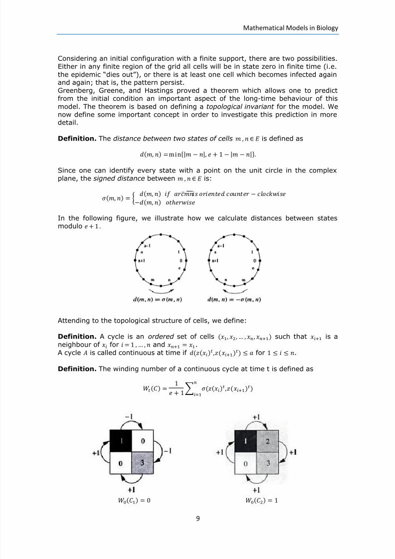
Definition. A cycle is an ordered set of cells such that is aneighbour of for and .A cycle is called continuous at time if for .

Definition. The winding number of a continuous cycle at time t is defined as




10

In the figure above, we give an example of two possible continuous cycles with fourdifferent cells ( ). The first one has winding number zero andthe other has winding number one. As a result of the following theorem, we will seethat different patterns occur and only a cycle with nonzero winding number ensures

persistence.Greenberg, Greene and Hastings theorem. Given a Greenberg-Hastingsautomaton with ⁄ , a configuration with finite supportis persistent if and only if , for some continuous cycle.

Back to our example, we will show the patterns at 0, 13, 14, 15, 16 and 17iterations using the previous cycles as initial conditions.

In the case of , an epidemic wave travels once across the grid and the dies out:

In the case of , it leads to persistence of the epidemic and a periodic patternevolves.

So, to achieve persistence we have to ensure that susceptible cells of a cycle will beinfected again.

Relation to an SIR Model

Consider the Kermack-McKendrick ODE Model:

̇ ̇ ̇where is the incidence function, is the rate of immunization and is therate of recovery.

The similarities one can observe between both models are: , the mean time anindividual stays in the infectious class, corresponds to . Analogously, corresponds to the number of recovery states .

On the other hand, the main difference is the relation between the incidencefunction and the infection rules. In the classical Kermack-McKendrick model, a massaction term is chosen, . This means that the individuals are well




11

mixed, and every susceptible has the same chance to be infected. As we said, inGreenberg-Hastings automaton, infectious cells can only infect neighbouringsusceptibles.

However, we can approximate each model with the other. Introducing a spatialmixing rule in the Greenberg-Hastings automaton, it leads to the ODE model and inthe other way, different incidence functions can be considerated to include theeffect of local infection.

References

[1]”A Course in Mathematical Biology : Quantitative Modeling with Mathematical andComputational Methods ” G. de Vries, T. Hillen, M. Lewis, J. Müller, B. Schönfisch.[2]"University and Complexity in Cellular Automata" [Physica D 10 (1984) 1-35]

[3] http://mathworld.wolfram.com[4] Greenberg, J, Greene, C., and Hastings, S.P., ”A combinatorial problem aris ingin the study of reaction-diffusion equations ” , Siam J. of Algebra and DiscreteMethods vol. 1, (1980), 34-42.[5] http://en.wikipedia.org/wiki/Cellular_automaton

CA Models for Epidemic Diseases

Documents

Transcript of CA Models for Epidemic Diseases