Bump at the End of the Bridge Enhanced Remediation Decision Making via 3D Measurement and Advanced 3D Dynamic Analysis Research Final Report from The University of Memphis | Charles V. Camp, Shahram Pezeshk, Ali Kashani, and Donny Dangkua | August 31, 2021

Sponsored by Tennessee Department of Transportation Long Range Planning

Research Office & Federal Highways Administration

i

DISCLAIMER This research was funded through the State Planning and Research (SPR) Program by the Ten-nessee Department of Transportation and the Federal Highway Administration under RES 2019-21: Bump at the End of the Bridge: Enhanced Remediation Decision Making via 3D Measurement and Advanced 3D Dynamic Analysis.

This document is disseminated under the sponsorship of the Tennessee Department of Trans-portation and the United States Department of Transportation in the interest of information ex-change. The State of Tennessee and the United States Government assume no liability of its con-tents or use thereof.

The contents of this report reflect the views of the author(s) who are solely responsible for the facts and accuracy of the material presented. The contents do not necessarily reflect the official views of the Tennessee Department of Transportation or the United States Department of Trans-portation.

ii

Technical Report Documentation Page

1. Report No. RES2019-21

2. Government Accession No. 3. Recipient's Catalog No.

4. Title and Subtitle

Bump at the End of the Bridge: Enhanced Remediation Decision Making via 3D Measurement and Advanced 3D Dynamic Analysis

5. Report Date July 2021

6. Performing Organization Code

7. Author(s) Charles V. Camp and Shahram Pezeshk

8. Performing Organization Report No.

9. Performing Organization Name and Address The University of Memphis3720 Alumni AveMemphis, TN, 38152

10. Work Unit No. (TRAIS)

11. Contract or Grant No. Grant RES2019-21

12. Sponsoring Agency Name and AddressTennessee Department of Transportation505 Deaderick Street, Suite 900Nashville, TN 37243

13. Type of Report and Period Covered Final Report December 2018 – August 2021 14. Sponsoring Agency Code

15. Supplementary Notes Conducted in cooperation with the U.S. Department of Transportation, Federal Highway Administration. A sup-plementary document with additional information is available upon request.

16. Abstract

The Tennessee Department of Transportation (TDOT) and transportation departments across the country havelong recognized that approach slabs and pavements at bridges are prone to both settlement and cracking, which have been widely recognized as the "bump at the end of the bridge" (BEB). This study seeks to provide guidance and aid TDOT officials in their decision-making process regarding potential BEB remediation strategies using non-destructive 3D subsurface measurements and advanced 3D dynamic analyses. An innovative strategy was utilized that combines survey data from multi-frequency ground penetrating radar (GPR) and multi-channel anal-ysis of surface waves (MASW) to develop accurate 3D subsurface soil maps of bridge approach slabs and foun-dations. PLAXIS 3D was used to developed sophisticated dynamic finite element (FE) models of the soil-structure system subjected to moving truckloads were developed for the bridge approach from the developed subsurface maps. The FE models were used as a framework for evaluating different remediation actions to address various types of BEB problems. For example, using these techniques, a PLAXIS 3D model was developed for the Horn Lake Creek Bridge to examine the effects of reinforcing the approach foundation. In this case, the foundation under the approach pavement was reinforced with geogrids as defined by TDOT in STD-10-2. Compared to an unreinforced foundation, the predicted pavement displacements at the soil-structure interface using geogrid rein-forcement were reduced by more than 40%. 17. Key Words

GROUND PENETRATING RADAR (GPR); MULTI-CHANNEL ANALYSIS OF SURFACE WAVES (MASW); 3D DY-NAMIC FINITE ELEMENT MODELS

18. Distribution Statement No restriction. This document is available to the public from the sponsoring agency at the website http://www.tn.gov/

19. Security Classif. (of this report) Unclassified

20. Security Classif. (of this page) Unclassified

21. No. of Pages 58

22. Price

iii

Executive Summary The Tennessee Department of Transportation (TDOT) and transportation departments across the country have long recognized that approach slabs and pavements at bridges are prone to both settlement and cracking, which have been widely recognized as the "bump at the end of the bridge” (BEB). The primary objective of this study was to provide guidance and aid TDOT officials in their decision-making process regarding bridge approach remediation via an improved under-standing of BEB issues. The research activity had the following two specific objectives:

1. Conduct 3D subsurface measurements using a combination of ground-penetrating radar (GPR) and multi-channel analysis of surface waves (MASW) to delineate soil layers, and

2. Develop advanced 3D dynamic analyses of the approach slab and pavement using the subsurface maps.

Detailed 3D subsurface maps of the approach slab and pavement at four bridges in Shelby County, Tennessee, were developed using a combination of GPR and MASW data. These 3D sub-surface maps were used to developed sophisticated finite element (FE) models of the soil and pavement systems under dynamic loading. These models' results help understand current bridge conditions and provide a framework for evaluating different mitigation and repair strategies.

An innovative strategy three-stage procedure was used to develop 3D subsurface soil models. At each bridge approach site, data were collected using GPR and MASW. In Stage 1, MASW data was recorded in the middle of each lane at the entrance and exit zones of the bridge and analyzed to estimate the shear-wave velocity. In Stage 2, GPR data was collected using 100 MHz and 500 MHz antennae. In Stage 3, a 3D subsurface soil model was developed using MASW results to adjust the soil velocity for the GPR test and accurately measure each soil layer's depth and thickness.

For the MASW surveys, a set of 24 geophones were used along a longitudinal section of a bridge approach slab and pavement. At each bridge site, thirteen arrays of 24-channel were recorded for each lane. The data collected from each field setup were processing to generate a dispersion image at the mid-point of the array. Each of the thirteen dispersion curves was then inverted to solve for 1-D shear wave velocity profiles at the mid-point of the array. The resulting thirteen 1-D shear wave profiles are then integrated to develop 2-D shear wave velocity. A 3-D shear-wave velocity model was developed using a 3D Delaunay triangulation based on the 1-D velocity pro-files as input points.

The GPR surveys were conducted along a gridline system drawn on the roadway surface using a 5 ft. interval between lines along longitudinal and traverse to the pavement. GPR data were col-lected along each grid line using a 500 MHz antenna for shallower depths (up to 1 m) and a 100 MHz antenna to survey deeper depths (up to 10 m). The 2D GPR images were located within the gridline system to form a partial 3D subsurface survey. The MASW results were used to adjust the shear wave velocity of the 2D GPR images and accurately estimate the depth and thickness of each soil layer within the gridline system. A 3D soil model was generated by interpolating the gridline data using an open-source, multi-platform data analysis and visualization application.

The 3D subsurface models developing using MASW and GPR surveys were used to develop PLAXIS 3D simulations of the approach slab and pavement under dynamic loadings. Dynamic loads were based on the American Association of State Highway and Transportation Officials

iv

(AASHTO) HL-93 design truckloads. The PLAXIS 3D models provided a framework to evaluate the dynamic effects on displacement and stress in the bridge and surrounding soil foundation due to moving truckload loadings. A PLAXIS 3D model was developed for the Horn Lake Creek Bridge (Bridge #79-175-0.18) located in Shelby County, Tennessee, to examine the effects of reinforcing the approach foundation. For this case, the original PLAXIS 3D model was compared to one where the foundation under the approach pavement was reinforced with geogrids as defined by TDOT in STD-10-2. The PLAXIS 3D results predicted an 85% reduction in maximum displacement and a 70% reduction in absolute stress at the soil-structure interface for the reinforced foundation. Also, there was about a 40% reduction in the maximum displacement and a 48% reduction in the maximum principal stress throughout the entire model.

Key Findings • Non-destructive 3D subsurface surveys provide information on the current state of bridge

approach foundations for assessing BEB issues • Accurate 3D soil maps were be developed by combining MASW and GPR data • Dynamic PLAXIS 3D models of the bridge approach system were developed from the 3D

surveyed 3D soil maps • The resulting dynamic PLAXIS 3D models can provide a platform for evaluating BEB miti-

gation strategies and alternative retrofit designs

Key Recommendations • Combine MASW with GPR to provide an effective non-destructive method for developing

accurate 3D subsurface surveys • Use MASW and GPR surveys to provide an additional level of quality control on new con-

struction • Consider the results from 3D soil-structure models when evaluating alternative BEB miti-

gation strategies

v

Table of Contents DISCLAIMER .................................................................................................................................................. i

Technical Report Documentation Page ................................................................................................... ii

Executive Summary ................................................................................................................................... iii

Key Findings ........................................................................................................................................... iv

Key Recommendations ......................................................................................................................... iv

List of Tables ............................................................................................................................................. vii

List of Figures ........................................................................................................................................... viii

Chapter 1 Introduction........................................................................................................................ 1

Chapter 2 Literature Review ................................................................................................................ 3

2.1 Causes of BEB Problem ................................................................................................................... 3

2.2 Mitigation Techniques ..................................................................................................................... 4

2.3 Approach Slab Stiffness ................................................................................................................... 5

2.4 Drainage Improvement and Erosion Mitigation .......................................................................... 5

2.5 Retrofitting Techniques ................................................................................................................... 5

2.6 Integral Abutment Bridges .............................................................................................................. 5

Chapter 3 Methodology ....................................................................................................................... 7

3.1 Multi-channel Analysis of Surface Waves (MASW) ....................................................................... 7

3.1.1 MASW Equipment ........................................................................................................................ 7

3.1.2 Trigger Effect and Stacking ........................................................................................................ 10

3.1.3 MASW Testing Procedure .......................................................................................................... 10

3.1.4 MASW Date Analysis .................................................................................................................. 11

3.2 Ground Penetration Radar (GPR) ................................................................................................. 14

3.2.1 GPR Limitations .......................................................................................................................... 15

3.2.4 GPR Data Collection Method ..................................................................................................... 16

3.2.5 GPR Data Analysis ...................................................................................................................... 20

3.2.6 Data Analysis Using EKKO Project Software .............................................................................. 21

3.3 PLAXIS 3D Modeling ....................................................................................................................... 30

3.4.1 Modeling Basic Principles .......................................................................................................... 31

3.4.2 PLAXIS 3D ................................................................................................................................... 33

Chapter 4 Results and Discussion .................................................................................................... 35

4.1. 3D Subsurface Soil Maps.............................................................................................................. 35

4.2. 3D Dynamic Analysis..................................................................................................................... 36

vi

4.3. Evaluation of Soil Reinforcement ................................................................................................ 42

Chapter 5 Conclusion ......................................................................................................................... 45

Key Recommendations ........................................................................................................................ 45

References ................................................................................................................................................. 47

vii

List of Tables TABLE 3-1. ...................................................................................................................................................................... 32 TABLE 3-2. ...................................................................................................................................................................... 33 TABLE 4-1 ....................................................................................................................................................................... 36

viii

List of Figures Figure 2-1. Illustration of bump mechanics [7] .............................................................................................................. 4 Figure 2-2. Thermal effects on the bridge and integral abutment [15] ......................................................................... 6 Figure 3-1. Depth sampled by Rayleigh waves with different wavelengths [18] .......................................................... 8 Figure 3-2. Variation of horizontal and vertical normalized components of displacements induced by Rayleigh waves

with normalized depth in a homogeneous isotropic, elastic half-space ............................................................... 8 Figure 3-3 Vertical geophone with a corner frequency of 4.5 Hz .................................................................................. 9 Figure 3-4. Geophone cable: (a) red end-connection and the yellow slot for geophone hookup, (b) black end-

connection, and (c) details of the end-connection ............................................................................................... 9 Figure 3-5. Geometrics Geode 24 channel digitizer ...................................................................................................... 9 Figure 3-6. Data transfer cable from geode to geode, or from geode to software console on laptop ....................... 10 Figure 3-7. The trigger that attaches to the sledgehammer and signals the hit time ................................................. 10 Figure 3-8. Overall MASW setup [19] .......................................................................................................................... 11 Figure 3-9. MASW geophone setup ............................................................................................................................. 11 Figure 3-10. Dispersion image generated from analyzing the multi-channel records ................................................ 12 Figure 3-11. 1-D shear wave velocity profiles (solid line) inverted from the extracted dispersion curves based on the

initial model (dashed line) ................................................................................................................................... 13 Figure 3-12. 2-D shear wave velocity images developed from the 1-D shear wave velocity profiles ......................... 13 Figure 3-13. The 3-D shear wave velocity model ......................................................................................................... 14 Figure 3-14. Principle of GPR Data Collection [21] ...................................................................................................... 15 Figure 3-15. GPR equipment: (a) 100 MHz antennae; (b) 500 MHz antennae, and (c) controller [22][23] ................ 16 Figure 3-16. The concept of reflection and transmission ............................................................................................ 17 Figure 3-17. Point objects and the difference in reflections based on the material [24] ............................................ 17 Figure 3-18. Reflection of buried object [22] ............................................................................................................... 18 Figure 3-19. Surveying strategy based on pseudo-grid on a semi-random path [25] ................................................. 19 Figure 3-20. Surveying strategy based on grid line path [23][25]................................................................................ 20 Figure 3-21. Gridlines for GPR data collection on the Horn Lake Creek Bridge ........................................................... 21 Figure 3-22. The EKKO Project view of data collected the 500 MHz GPR antenna ..................................................... 22 Figure 3-23. GPR images using a 500 MHz antenna along the X-direction ................................................................. 23 Figure 3-24. GPR images along the Y-direction lines on the concrete approach path ................................................ 24 Figure 3-25. GPR images along Y-direction lines on the road surface ......................................................................... 25 Figure 3-26. MASW profile for the exit zone of the Horn Lake Creek Bridge .............................................................. 26 Figure 3-27. Soil layer delineations 500 MHz antennae along the X-direction ........................................................... 27 Figure 3-28. The 2D surface at the depth levels near the first layer ........................................................................... 28 Figure 3-29. The 2D surface at the depth levels near the first layer ........................................................................... 29 Figure 3-30. The 3D model for Horn Lake Creek Bridge using Paraview software. ..................................................... 30 Figure 3-31. Problems Leading to the Existence of a Bump [38] ................................................................................. 32 Figure 3-32. The cross-section of the Horn Lake Creek Bridge (provided by TDOT) ................................................... 33 Figure 3-33. AASHTO HL-93 design truckload [40] ...................................................................................................... 34 Figure 3-34. Maximum pavement deflections due to moving loads ........................................................................... 34 Figure 4-1. 3D soil layer model for I-269 at Fletcher Creek Bridge .............................................................................. 36 Figure 4-2. Position of AASHTO HL-93 truckloads with time ....................................................................................... 37 Figure 4-3. Maximum pavement deflections due to moving loads ............................................................................. 38 Figure 4-4. Pavement deflection contours due to moving loads ................................................................................. 40 Figure 4-5. Displacement at soil-structure interface ................................................................................................... 41 Figure 4-6. Stress at soil-structure interface ............................................................................................................... 41 Figure 4-7. TDOT STD-10-2 Misc. Abutment & Pavement at Bridge Ends Backfill Details 2020 .................................. 42 Figure 4-8. Displacement at the soil-structure interface for reinforced and unreinforced foundations .................... 42 Figure 4-9. Change in displacement at the soil-structure interface for reinforced and unreinforced foundations .... 43 Figure 4-10. Stress at the soil-structure interface for reinforced and unreinforced foundations ............................... 43

1

Chapter 1 Introduction Transportation departments across the country have long recognized that approach slabs and pavements at bridges are prone to both settlement and cracking, which have been established as the "bump at the end of the bridge" (BEB). Bridge approach span problems affect about 25% of U.S. bridges, and hundreds of millions of dollars have been spent on repairs dealing with this issue [1].

A bump often develops at the end of a bridge near the abutment and embankment interface. Reduction in steering response, the distraction of driver, maintenance cost, citizen dissatisfac-tion, and negative perception are all undesirable effects of BEB.

The difference in elevation between the approach pavement and the bridge deck is a complex problem involving the interaction of many components. According to the National Cooperative Highway Research Program (NCHRP) Synthesis 234 report [1], the most commonly reported con-tributing factor of the bump are the interaction of the bridge structure, backfill soils, and foun-dation soils; inadequate drainage; settlement of the natural soil under the embankment; poor construction practices; high traffic loads; inferior fill materials, loss of fill by erosion; poor joints; temperature cycles. The settlements can result in unsafe driving conditions, rider discomfort, structural deterioration of bridges, and long-term maintenance costs.

The Tennessee Department of Transportation (TDOT) routinely receives complaints from motor-ists about BEB issues at the bridge and roadway interface. The problems related to the BEB have been the subject of numerous research and investigations. Despite these research efforts, the characterization and identification of the underlying issues that cause BEB are problematic, which impedes remediation efforts.

This study utilized an innovative strategy that combines data from multi-frequency ground pen-etrating radar (GPR) and multi-channel analysis of surface waves (MASW) to develop 3D subsur-face maps of bridge approach slabs and foundations. Advanced finite element (FE) models sub-jected to dynamic moving truckloads were developed for the bridge approach from the subsur-face maps. Combining the 3D subsurface maps and FE model provides a general framework for evaluation issues ranging from structural rehabilitation, maintenance options, and repair strate-gies. Also, the 3D maps and FE models provide information on the current conditions of the bridge approach and some insight on understanding the root causes for approach slab issues.

This research project was organized around four related tasks. First, perform non-destructive 3D measurements of road-bridge interface structure and supporting foundation for bridges with varying BEB problems and bridges without bump problems. Next, develop detailed 3D subsur-face models and use them to establish the current condition of the foundation and examine the potential causes of the BEB issues. Then, use the subsurface model to develop advanced 3D finite element (FE) analyses of the bridge approach system subjected to dynamic vehicle loadings. Lastly, use the FE models as a framework for evaluating different remediation actions to address various types of BEB problems.

2

In Chapter 2, a brief review of published literature is presented that defines the scope and extent of the BEB problem throughout the U.S. and summarizes crucial causes and effective mitigation and retrofitting techniques. A general introduction to GPR and MASW techniques and the associ-ated data analysis and details on the FE modeling process is discussed in Chapter 3. The devel-oped 3D subsurface models and FE model results for all surveyed sites are presented in Chapter 4. The FE models form the framework for evaluating different design strategies and remediation actions.

3

Chapter 2 Literature Review Differential settlements between bridge deck or abutment and approach pavement at both ends of bridges are referred to as the bump at the end of the bridge (BEB). In general, the two main conditions that cause BEB to occur are the change in the slope at the approach slab-bridge deck interface and the soil-structure boundary at the approach slab-roadway pavement interface. At first glance, it may not be a serious structural problem, though many complaints have been re-ported about rider discomfort when entering and exiting the bridges. Besides, the BEB can result in unsafe driving conditions, structural deterioration of bridges, and long-term maintenance costs.

Based on a highway survey conducted by Briaud et al. [1], about 150,000 out of 600,000 US high-way bridges (as of 1995), nearly 25%, experienced BEB problems. According to Wahls [2], differ-ential settlements over ½-inch are noticeable by driving public. As differential settlements at the bridge abutment increase, the potential risk of vehicle damage and accidents due to loss of con-trol become a significant concern [3][4]. Once the bridge approach settlement becomes unac-ceptable, state Departments of Transportation (DOTs) need to repair or reconstruct the bridge approach.

The difference in elevation between the approach pavement and the bridge deck is a complex problem involving the interaction of many components. According to the National Cooperative Highway Research Program (NCHRP) Synthesis 234 report [1], the most commonly reported con-tributing factor of the bump are the interaction of the bridge structure, backfill soils, and foun-dation soils; inadequate drainage; settlement of the natural soil under the embankment; poor construction practices; high traffic loads; inferior fill materials, loss of fill by erosion; poor joints; temperature cycles [5].

Numerous comprehensive studies of mitigation related to the BEB have been sponsored over the years by various state DOTs and the Federal Highway Administration (FHWA). The effects of embankment and foundation settlement on the approach settlement depend on conditions at the bridge site.

In a nutshell, after reviewing previous studies, the most crucial causes and the most effective mitigation and retrofitting techniques can be summarized as follows.

2.1 Causes of BEB Problem The BEB problem is generally attributed to the differential settlement between the approach slab or pavement and bridge abutment [6]. Figure 2-1 illustrates two different kinds of bumps that occur due to differential settlements, one at the connection of approach slab and pave-ment (Bump 1) and the other at the intersection of bridge and approach slab (Bump 2). The root causes of differential settlement can be the following: settlement of the natural soil, poor construction practices, compression of the fill material, poor fill material, high traffic loads, ero-sion, and degradation of expansion joints [5].

4

Figure 2-1. Illustration of bump mechanics [7]

2.2 Mitigation Techniques Many researchers have investigated methods to relieve the BEB problem, primarily by reducing differential settlement.

A. The quality of fill material. Several considerations were suggested for minimum grading requirements based on the area where the bridges are constructed. Some general rec-ommendations are using granular or non-cohesive soils over cohesive soils [8]. In cohe-sionless soil, settlement of foundation soil is not usually time-dependent. During con-struction, when dead loads are applied gradually, settlements can be observed. So, the main difference is time; in cohesionless soil long term settlement is absent.

B. The compaction of fill material. To be more exact, the more compacted the material, the less the differential settlement. However, this would not be an easy task when the aim is the compaction of the backfill behind the abutment and beneath the approach slab [5]. Two solutions were proposed for this problem [9]: 1) constructing the abutment without any notches and overhangs, and 2) giving enough time to the soil to settle as much as possible.

C. The use of predictive techniques. Evaluating soil conditions and treatments can provide enough information to design sub-structural elements tied to the bump problems.

D. The use of geosynthetic material helps to reduce the settlement and increase the soil's bearing capacity. Successful applications of geosynthetics have been reported since the 1980s [10]. Some researchers recommended combining geosynthetic reinforcement with a polyethylene sheet or filter fabric underneath the approach slab [11].

E. Improving the foundation soil. For example, removing and replacing the weak soil, using chemicals (e.g., deep soil mixing or grout or lime stabilization), surcharging, and deep foundations [12].

In 2020, TDOT updated its standard structural drawings (STD 10-2 and STD 10-3) for abutments and pavements to include additional requirements and details for backfill and ditches at the

5

bridge end to mitigate excessive settlement. For backfill, TDOT requires four 9 in. layers of ge-otextile and geogrid reinforcement wrap at the face of the abutment and wingwalls over the approach slab and the first 15 ft. of the pavement.

2.3 Approach Slab Stiffness In an investigation conducted by Louisiana Transportation Research Center, increasing the ap-proach slab's flexural rigidity was shown to be an effective way of controlling settlement [7]. The focus of this technique was reducing the difference in flexural stiffness between the bridge and the embankment [9][13]. Abu-Farsakh and Chen [7] tried to overcome the stiffness issue by incorporating geosynthetic reinforcement into foundation soil.

2.4 Drainage Improvement and Erosion Mitigation Inadequate drainage systems, either on the surface or subsurface, play a pivotal role in the differential settlement [12][14]. Inefficient drainage systems cause differential settlement by making voids in the soil and resulting in settlement. Several recommendations to mitigate this issue are improved slope drainage systems [12], using geosynthetic reinforced backfill [14], and consistent maintenance of joints and drainage systems [8].

2.5 Retrofitting Techniques Several retrofitting techniques have been applied to BEB locations. The first method is lifting and realigning, where holes are drilled in the approach slab, and the voids are filled with sand, clay mixtures, or special foams [9]. Although some states used this methodology successfully, there are some drawbacks: 1) this technique does not work for large voids [10]; and 2) when drainage systems becoming clogged, it is difficult for them to be replaced [8]. A second faster and less expensive alternative is overlaying, where BEE is paved over and smoothed out [6]. Overlaying also increases the total weight and, consequently, the backfill stresses [10]. The third strategy is the complete replacement of the approach slab [12].

2.6 Integral Abutment Bridges In these bridges, the abutment and bridge deck are rigidly connected without expansion joints. In this case, construction and maintenance costs are reduced while improving seismic perfor-mance since the abutment and the deck work as a single structure [15]. Despite successful applications of these solutions, the BEB problem can reoccur in these structures due to cycling loadings. For instance, as shown in Figure 2-2, thermal-induced cyclic loads cause expansion and contraction movements and finally result in voids behind the abutment and beneath the approach slab [16][17].

6

Figure 2-2. Thermal effects on the bridge and integral abutment [15]

In addition, the movement of the abutment can induce lateral earth pressure on the abutment [17]. All of these conditions cause settlement of the approach slab and damage to the abutment back wall. Many solutions have been proposed to reduce this issue: using an expansion joint at the end of the approach slab [13], using geosynthetic reinforcement and a spacer [10], and using polyethylene sheets to decrease friction from horizontal movements [11].

7

Chapter 3 Methodology Detailed information on the methodology and equipment required to develop 3D surface profiles and perform 3D dynamic analysis of bridge approach systems proposed in this study are listed below. Multi-channel analysis of surface waves (MASW) was used to evaluate soil profiles' struc-tural and dynamic properties. Accurately estimating soil properties is critical in developing dy-namic models of bridge-roadway interface for both static and dynamic loadings.

Ground penetrating radar (GPR) is the general term for techniques that employ radio waves in the range of 1 to 2,000 MHz frequencies and map structures and features in man-made struc-tures and soil profiles. GPR is a non-destructive technique in which radar is transmitted into the ground using an antenna pushed across the ground surface. The radar travels through underly-ing materials and is reflected by subsurface features. The results from MASW are combined with GPR data to develop 3D subsurface models delineating soil layers.

The 3D subsurface maps established from MASW and GPR surveys were used to develop PLAXIS 3D simulations of the approach slab and pavement under dynamic loadings. PLAXIS 3D is a state-of-the-art three-dimensional FE analysis for complex geotechnical problems, capable of predict-ing differential settlements and stresses under time-dependent loadings for multi-layered soil foundations.

3.1 Multi-channel Analysis of Surface Waves (MASW) Rayleigh waves generate a circular particle motion in an infinite half-space. This motion's am-plitude is an exponential function that is tied to frequency and wavelength. The lower frequen-cies (longer wavelengths) have a more extensive range of motion, and higher frequencies (shorter wavelengths) have a smaller range of particle motion. Consequently, higher frequency Rayleigh waves sample shallower depths and lower frequencies sample deeper through the soil layers, as shown in Figure 3-1. Knowing the velocity of seismic waves is a function of soil shear-wave velocity. We can find out that different frequency ranges (phases) of Rayleigh waves travel at different phase velocities since they sample different soil layers with other seismic characteristics. This effect is called the dispersion of surface waves. Figure 3-2 shows the nor-malized vertical and horizontal particle motion exponentially decreasing with depth.

The entire data processing sequence, from generating dispersion image, picking dispersion curve, inverting dispersion curve to obtain 1-D shear wave velocity profile, and developing 2-D shear wave velocity image, were performed using SurfSeis MASW software the Kansas Geolog-ical Survey.

3.1.1 MASW Equipment MASW equipment consists of the following:

• Vertical geophones to convert surface perturbations into electric analog signals (Figure 3-3)

• Geophone cables for all 24 geophones to transmit the electrical signals to the digitizing unit (Figure 3-4)

• Digitizing units that transform the electric analog signal into digital data recordable as a computer file; three (3) Geometrics Geodes® were used for this study (Figure 3-5)

8

• Data cables to transfer the digitized data into a PC (Figure 3-6) • A laptop connected to the data cable to record incoming digitized signals into data files • A software console handling communication with the digitizers, recording the digitized

signals into a file, and setting parameters related to the experiment • A source of energy like a sledgehammer • A trigger attached to the hammer and an extension cable to connect the trigger to the

digitizer (Figure 3-8)

Figure 3-1. Depth sampled by Rayleigh waves with different wavelengths [18]

Figure 3-2. Variation of horizontal and vertical normalized components of displacements induced by Ray-leigh waves with normalized depth in a homogeneous isotropic, elastic half-space

10

Figure 3-6. Data transfer cable from geode to geode, or from geode to software console on laptop

Figure 3-7. The trigger that attaches to the sledgehammer and signals the hit time

3.1.2 Trigger Effect and Stacking Considering the presence of noise in the recorded data, it is common practice to repeat each hit several times and stack the recorded data so that the random nature of the noise results in the cancellation of the noise and the strengthening of the signal. It is expected that when a trigger is used, all data recorded at a different hit have the same signal, which can be added point by point.

3.1.3 MASW Testing Procedure Figure 3-8 illustrates the overall MASW setup. A 10-lb sledgehammer was used to generate sur-face waves with a source offset of 6 ft. from the first receiver. The propagating surface waves were recorded using 24 4.5 Hz-vertical geophones with a receiver interval of 3 ft. The survey was performed in roll-over push mode every 3 ft. to develop two-dimensional shear wave ve-locity profiles. Three records are acquired at all locations and then summed into one to sup-press the urban ambient noise.

9

Figure 3-3 Vertical geophone with a corner frequency of 4.5 Hz

Figure 3-4. Geophone cable: (a) red end-connection and the yellow slot for geophone hookup, (b) black end-connection, and (c) details of the end-connection

Figure 3-5. Geometrics Geode 24 channel digitizer

Once the test setup is complete, Rayleigh waves are generated by striking a metal plate with a sledgehammer at a specific location. The trigger signals the digitizer to start recording at the onset of hit time, and the digitizer sends the data from the geophones to the software console on the laptop.

11

Figure 3-8. Overall MASW setup [19]

Figure 3-9 shows a typical set of 24 geophones along a longitudinal section of a bridge approach slab and pavement. At each bridge site, thirteen arrays of 24-channel were recorded for each lane. The data collected from each field setup were processing to generate a dispersion image at the mid-point of the array. An example of a single acquired multi-channel record is shown on the right-hand side of Figure 3-8.

Figure 3-9. MASW geophone setup

3.1.4 MASW Date Analysis Figure 3-10 shows an example of a dispersion image generated from multi-channel records using the SurfSeis MASW Software. The dispersion curve (indicated by the white squares in Figure 3-10) is extracted based on the peak amplitude level in the image.

12

Figure 3-10. Dispersion image generated from analyzing the multi-channel records

13

The dispersion curves are then inverted to solve for a 1-D shear wave velocity profile at the mid-point of the array. Figure 3-11 shows 1-D shear wave velocity profiles for a point on a bridge approach slab.

Figure 3-11. 1-D shear wave velocity profiles (solid line) inverted from the extracted dispersion curves based on the initial model (dashed line)

The 1-D shear wave profiles are then used to develop 2-D shear wave velocity images, as shown in Figure 3-12. In this example, the bridge was located on the left side of the image. It can be observed from Figure 3-12 that there was a low-velocity layer (up to 600 ft/s) at the surface, followed by a higher velocity layer (600-1,200 ft/s). Another low-velocity layer below is followed by another higher velocity layer down to the bottom of the profile. Also, the top three layers are dipping down at the interface with the bridge.

Figure 3-12. 2-D shear wave velocity images developed from the 1-D shear wave velocity profiles

The 1-D shear wave velocity profiles were used to develop the 3-D velocity model using the ParaView visualization software [20]. A 3-D shear-wave velocity model was developed using a filter that constructs a 3D Delaunay triangulation based on the 1-D velocity profiles as input

14

points. Figure 3-13 shows an example 3-D shear wave velocity model for the subsurface of a bridge approach.

Figure 3-13. The 3-D shear wave velocity model

3.2 Ground Penetration Radar (GPR) New and advanced software and equipment now provide cost-effective procedures to identify existing underground utilities, pavement, and soil information to the desired depth. GPR is the general term for techniques that employ radio waves in the range of 1 to 2,000 MHz frequencies and map structures and features in man-made structures and soil profiles. GPR is a non-de-structive technique in which radar is transmitted into the ground using an antenna pushed across the ground surface. The radar travels through underlying materials and is reflected by subsurface features. The magnitude of the reflections is based on contrasts in dielectric con-stant (a dimensionless unit that is a measure of the capacity of a material to store charge when an electric field is applied) and electrical conductivity of the subsurface features. Subsurface voids or other subsurface features may be detected based on the dielectric constant between soil and air-filled void space or obstructions. The time required for the reflected signal to travel down and back is recorded. GPR surveying can be conducted using various antenna frequen-cies, generally ranging between 100 MHz and 2,000 MHz. Generally, lowering frequency im-proves the depth of exploration because attenuation primarily increases with frequency, as shown in Figure 3-14. Typically, pavement-related investigations related to shallower features may be resolved using higher frequency antennae.

15

Figure 3-14. Principle of GPR Data Collection [21]

A GPR system is comprised of three main components: i) control unit, ii) antenna, and iii) power supply. The control unit is an electronic device used to operate and manage the data collection process. It consists of the digital video logger (DVL), battery, and power cables for connecting to antennas and transducers. A series of images are captured from pulses of radar energy that are triggered by the DVL unit. The triggering progress can be set manually, automatically using a preset interval time, or mechanically while moving the equipment. The antenna amplifies the triggered signals and sends them into the ground. DVL also has a built-in computer and memory to store data for processing after fieldwork. Figure 3-15 shows that both 500 MHz and 100 MHz antennae were used for the subsurface survey of all bridge approaches. The 500 MHz system was used to provide subsurface information just below the pavement, and the 100 MHz system was used to survey deeper depths (up to 10 m).

3.2.1 GPR Limitations GPR cannot identify a buried object based solely on reflected image. For example, rounded linear shapes whose diameters are about the same at the same depth level or the same diam-eters at different depth levels would produce similar images and requires other complemen-tary information to complete the survey. GPR penetration depth depends directly on the fre-quency of the antenna and the dielectric conductivity of the materials. The moisture content of the ground can be misleading in data interpretation. The velocity of the waves changes based on the material properties and can lead to different interpretations of the depth where an ob-ject is located.

16

Figure 3-15. GPR equipment: (a) 100 MHz antennae; (b) 500 MHz antennae, and (c) controller [22][23]

3.2.4 GPR Data Collection Method GPR maps the subsurface by producing a 2D image of the depth along a surveyed line on the surface by emitting a set of signals through a material over a given time interval and recording the strength and the travel time of any reflected waves. Reflections occur when the transmitted pulse encounters a material with different electrical conductivity. The strength of the reflection is a function of the contrast in the dielectric permittivity of the two materials. While some of the GPR energy pulses are reflected to the antenna, energy also keeps traveling through the mate-rial until it either dissipates (attenuates), or the GPR control unit has closed its time window.

17

Reflection works in the same way that a piece of glass mirrors an image while the object can be seen from the other side (reflection and transmission simultaneously, as shown in Figure 3-16).

Figure 3-16. The concept of reflection and transmission

The percentage of the reflected energy is defined using the reflection coefficient R given as

where K1 and K2 are the relative permittivities of the two materials.

Metals are complete reflectors and do not allow any amount of signal to pass through. Materi-als beneath a metal sheet, fine metal mesh, or pan decking are not visible. The final 2D image is obtained by putting these reflections together over a single surveyed line. The quality of the GPR image is affected by the number of transmitted signals.

As shown in Figure 3-17, point objects (i.e., something with a different material from the sur-rounding area or rod-like material such as pipe, wire, tree roots, etc., in the perpendicular di-rection to the survey line) emerged as arch-shaped images on the screen. These arches are produced because GPR signals emitted from the antenna travel into the ground like a 3D cone. The two-way travel time for energy at the leading edge of the cone is longer than for energy directly beneath the antenna. Therefore, the images' reflections appear even though an object is not directly located below the GPR sensor.

Figure 3-17. Point objects and the difference in reflections based on the material [24]

18

Thus, an object can be seen at some distance before and after the sensor goes over the top of it (see Figure 3-18). The top of the arch is the object's position, and the depth to the top of the arch is an estimated depth. GPR is a highly accurate device for locating different objects under the ground. The buried items appear on the computer screen in real-time as the GPR equip-ment moves along. Hence, their locations on the ground surface can be detected precisely by moving the GPR back and forth. Moreover, the material (metallic or non-metallic), the shape (circular, square, or jagged), and the direction (perpendicular to the survey line direction or inclined) of the objects can even be detected in some special cases based on the features of reflections.

Figure 3-18. Reflection of buried object [22]

The depth of an observed object is based upon the material being surveyed (different types of soil and asphalt, rock, etc.) because of the change in the signal velocity. The depth D of an object can be computed as

where V is the velocity of the wave and t is the travel time for a wave to go toward the object and coming back to the antenna. The factor of 2 in the denominator of Equation (2) accounts for the travel time to and from the object. Therefore, it is vital to calibrate the velocity (soil type calibration) and set it accurately during the analysis. Soil type calibration can be performed by: (i) matching the shape of a target arch, (ii) using a target at a known depth, and (iii) using the moisture level of the soil.

To start using the GPR, we assembled all the device parts and set all appropriate parameters based on the manufacturing recommendations for utilized antenna frequency and target ma-terials. The effective parameters that should be set in the control unit before running the test are 1) antenna frequency, 2) time window, 3) temporal sampling interval, 4) antenna separation, 5) antenna step size, 6) radar velocity, and 7) system stacking. The time window determines how long the radar system probes the subsurface that should be set based on the capacity of the antenna and the depth of the survey target. The GPR system samples the signals returning to the receiver in a series of numbers representing signal amplitude at equally spaced time intervals. The temporal sampling interval is the time interval between points on the trace. Se-lecting too large an interval makes the data under-sampled, which does not accurately repre-sent the actual signal. At the same time, too small an interval increases the data volume unnec-

19

essarily and slows down the data collection process. Antenna separation is the distance be-tween transmitter and receiver. If the distance between the antennas is too small, the receiver is overloaded by the transmitted signals, resulting in data clipping. Antenna step size deter-mines the distance the antenna pair should be moved each time to collect a new trace. Radar velocity depends on the wave propagation speed in different materials. System stacking im-proves the signal to noise, which means collecting more than one trace at each survey position. Manufacturers usually provide recommended values for these parameters in their technical manuals.

Several strategies are typically used for data collection: 1) line data, 2) pseudo-grid data, and 3) grid data. In the first strategy, data is along a line and viewed as a cross-sectional image. A buried object would appear as a hyperbolic image is approached at a transverse angle using this strategy. The second strategy collects data in a semi-random path to cover the whole area of interest, as shown in Figure 3-19. A third strategy is to draw a series of gridlines on the ground, and then data are collected independently along each grid line. Figure 3-20 shows a sample grid line system. In this study, we used a grid line system for all surveys.

Figure 3-19. Surveying strategy based on pseudo-grid on a semi-random path [25]

20

Figure 3-20. Surveying strategy based on grid line path [23][25]

3.2.5 GPR Data Analysis Analyzing and interpreting GPR data was the most critical step after data collection. In this pro-ject, we used the 100 MHz and 500 MHz antennas produced by Sensors and Software and the backup software for analysis called EKKO Project V5 R3. The 500 MHz antenna was utilized for the shallower data collection, while the 100 MHz antenna was selected for inspecting deeper soil layers. A critical step in the analysis is determining the velocity of waves in the soil based on the dielectric constant. Normally. A series of field and lab tests must be conducted to meas-ure the dielectric constant. In this study, we used a novel procedure for estimating velocity based on the MASW test results. We overlapped the GPR data with the soil stratification results from MASW and adjusted velocities until both data sets produced similar soil layer delineations. These velocities were then used to analyze the remainder of the GPR dataset.

A three-step procedure was used to develop 3D subsurface soil models. For each bridge ap-proach site, data were collected using 100 MHz and 500 MHz GPR antennas and MASW. The process for analyzing the data and generating a 3D model is listed as follows:

21

• Stage 1 (MASW test): 1) perform the test for the middle lane at each zone (entrance and exit zones of the bridge), and 2) capturing the soil stratification, the boundaries of chang-ing shear-wave velocity, and their depth.

• Stage 2 (100 MHz and 500 MHz tests): 1) a grid line system was drawn on the roadway with a 5 ft. interval between lines along longitudinal and traverse to the pavement, 2) GPR device was calibrated along a measured length, 3) along each grid line, data were collected for shallow depths using the 500 MHz antenna, and 4) data were collected along the same grid lines using the 100 MHz antenna to survey deeper depths.

• Stage 3 (3D model development): 1) MASW results were used to adjust the velocity for the GPR test to extract the soil layers' bounds and thickness, and 2) the GPR data was im-ported into Paraview, an open-source, multi-platform data analysis and visualization ap-plication, and a 3D soil model was generated.

3.2.6 Data Analysis Using EKKO Project Software The first bridge approach pavement surveyed was the northern end of Bridge #79-175-0.18 (SR 175 over Horn Lake Creek), located in Memphis, Tennessee. Figure 3-21 shows the general lay-out of the gridline system used to collect the GPR data. Gridlines were drawn on the pavement for the northern entrance and exit zones of the bridge. The gridlines oriented parallel with the roadway were donated as the X-lines, and those perpendicular to the roadway are Y-lines (see Figure 3-21). Figure 3-22 shows an example of data collected using the 500 MHz antenna for the Horn Lake Creek Bridge displayed in the EKKO Project software.

Figure 3-21. Gridlines for GPR data collection on the Horn Lake Creek Bridge

22

Figure 3-22. The EKKO Project view of data collected the 500 MHz GPR antenna

23

Figure 3-22 shows a series of captured GPR images along gridlines in the direction of the road-way (long lines in the X-direction) using the 500 MHz antenna.

The strong reflections in Figure 3-22 represent considerable differences between the dielectric constants of materials and objects. In all the figures, there are some continuous linear and some round shape reflections. Figure 3-23 shows GPR images along six X-direction lines where the red vertical line indicates the boundary between the roadway and bridge approach slab (BEB location). This area is observable in Figure 3-21, along a line where the pavement and concrete change colors. At the left side of the red line in Figure 3-23, the image of the concrete approach slab is visualized. The circular reflections in this area are the rebars in the reinforced concrete. The shadow of those reflections can be observed in the deeper layers, and while they follow the same pattern as the primary reflections, they have weaker reflections. Therefore, these must not be considered independent reflections. However, on the right side of this red line is a soil embankment. The first black straight line at the top of the image is the reflection of the ground surface. The other black lines beneath that line are the boundaries between dif-ferent soil layers in which the material properties changed.

Figure 3-23. GPR images using a 500 MHz antenna along the X-direction

24

Accurately interpreting the captured images required complementary data that were not avail-able; however, based on the well-established standards defined for the pavement design, we were to proceed with generating the 3D model. There were various layers within the pave-ment's first 1-meter depth (e.g., dressing, surface course, base course). However, it appears that the primary source of the bump was the settlement in the deeper layers, not the shallower ones. Therefore, we eliminate using the higher frequency antennas than 500 MHz to capture details of those shallower layers. Moreover, we used a 100 MHz antenna for the deeper layers, which is more efficient than 500 MHz at that level.

Figures 3-24 and 3-25 show the surveyed lines along the Y-direction on the concrete approach path and road surface, respectively. It should be noted that Figure 3-24(f) is right above the interface of the roadway and approach slab where a BEB problem exists.

Figure 3-24. GPR images along the Y-direction lines on the concrete approach path

25

Figure 3-25. GPR images along Y-direction lines on the road surface

26

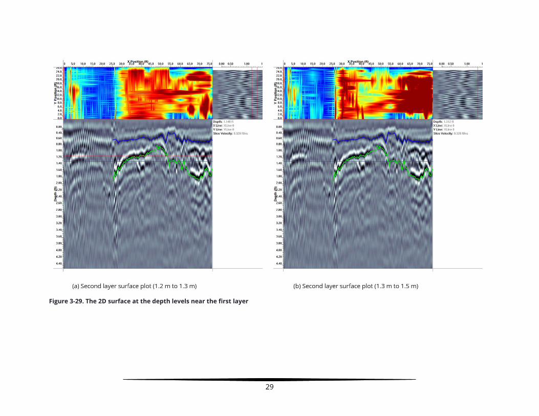
As shown in Figure 3-21, a grid strategy was used to develop 3D subsurface models. All the GPR surveys made along all the X and Y lines were georeferenced and combined, and the depths of soil layers at the intersection of those lines were extracted. Also, the MASW results (see Figure 3-26) were used to establish the wave's velocity and match the soil layer depths. The resulting model is like that shown in Figure 3-20(b). The velocity term for each line was adjusted. The boundary of a soil layer was located by comparing and matching MASW and GPR images along two perpendicular lines (one along X-direction and the other along the Y). Figure 3-27 shows the two top layers indicated by the blue and green lines. Soil settlement that potentially caused a BEB at the intersection of the roadway and bridge deck is indicated by the steep inclination of the green line in the second layer. Figures 3-28 and 3-29 show 2D surface plots at the depths of the first and second layers.

Figure 3-26. MASW profile for the exit zone of the Horn Lake Creek Bridge

27

Figure 3-27. Soil layer delineations 500 MHz antennae along the X-direction

28

Figure 3-28. The 2D surface at the depth levels near the first layer

29

Figure 3-29. The 2D surface at the depth levels near the first layer

30

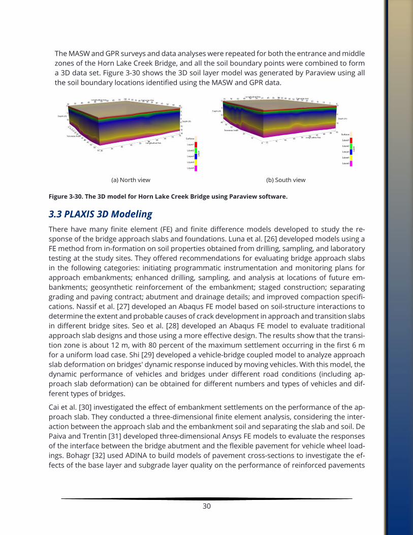
The MASW and GPR surveys and data analyses were repeated for both the entrance and middle zones of the Horn Lake Creek Bridge, and all the soil boundary points were combined to form a 3D data set. Figure 3-30 shows the 3D soil layer model was generated by Paraview using all the soil boundary locations identified using the MASW and GPR data.

Figure 3-30. The 3D model for Horn Lake Creek Bridge using Paraview software.

3.3 PLAXIS 3D Modeling There have many finite element (FE) and finite difference models developed to study the re-sponse of the bridge approach slabs and foundations. Luna et al. [26] developed models using a FE method from in-formation on soil properties obtained from drilling, sampling, and laboratory testing at the study sites. They offered recommendations for evaluating bridge approach slabs in the following categories: initiating programmatic instrumentation and monitoring plans for approach embankments; enhanced drilling, sampling, and analysis at locations of future em-bankments; geosynthetic reinforcement of the embankment; staged construction; separating grading and paving contract; abutment and drainage details; and improved compaction specifi-cations. Nassif et al. [27] developed an Abaqus FE model based on soil-structure interactions to determine the extent and probable causes of crack development in approach and transition slabs in different bridge sites. Seo et al. [28] developed an Abaqus FE model to evaluate traditional approach slab designs and those using a more effective design. The results show that the transi-tion zone is about 12 m, with 80 percent of the maximum settlement occurring in the first 6 m for a uniform load case. Shi [29] developed a vehicle-bridge coupled model to analyze approach slab deformation on bridges' dynamic response induced by moving vehicles. With this model, the dynamic performance of vehicles and bridges under different road conditions (including ap-proach slab deformation) can be obtained for different numbers and types of vehicles and dif-ferent types of bridges.

Cai et al. [30] investigated the effect of embankment settlements on the performance of the ap-proach slab. They conducted a three-dimensional finite element analysis, considering the inter-action between the approach slab and the embankment soil and separating the slab and soil. De Paiva and Trentin [31] developed three-dimensional Ansys FE models to evaluate the responses of the interface between the bridge abutment and the flexible pavement for vehicle wheel load-ings. Bohagr [32] used ADINA to build models of pavement cross-sections to investigate the ef-fects of the base layer and subgrade layer quality on the performance of reinforced pavements

31

under monotonic loading and study the effects of the interface friction between the geosynthet-ics and pavement layers. Gibigaye et al. [33] investigated the dynamic response of a pavement plate resting on the soil.

Madsen [34] develop a FE formulation for transient dynamic loading of a layered half-space is developed. Load speed was investigated, and the influence of the modulus ratio between the surface layer and the underlying soil for different load speeds was investigated. Ahirwar and Mandal [35] access the functioning of geogrids in the flexible pavement through FE analysis with PLAXIS 2D software. Their FE analysis results showed a reduction in vertical surface deformation when the geogrids were added between the pavement layers. Hu et al. [36] developed a 3D ABAQUS FE model to investigate and quantify the effects of tire inclination and dynamic loading on the stress-strain responses of a pavement structure under varying loading and environmental conditions.

3.4.1 Modeling Basic Principles One of the most critical factors in the development of BEB issues is the settlement of the abut-ment and embankment foundations. For example, long-term settlement can be an issue for silty and clayey foundations, while it is not the case for rock, gravel, or sand. Table 3-1 identifies a series of design considerations that contribute to the performance of a bridge approach [37][38]. Figure 3-31 illustrates factors involved in developing BEB problems [1][38]. Another factor is the potential settlement of the approach fill material. For example, fill materials that are adequately compacted can reduce the likelihood of large settlements. The abutment and wingwalls have two functions: 1) supporting the structural loads and 2) retaining the approach embankment. The types of abutment and the sequence of its construction can affect the de-velopment of BEB issues. Joints in the concrete pavement can cause BEB problems if not im-properly constructed or maintained.

The 3D subsurface soil model developed using both the GPR and MASW surveys highlighted the importance of fill material settlement. In this study, the factors listed in Table 3-1 were as-sumed to be adequately considered in the bridge design and that there were no issues during construction. Also, the soil embankments adjacent to an abutment wall were included in the dynamic analysis of the bridge. The soil is confined from the lateral movements, and the wall is modeled as a rigid element. The bridge superstructure is prevented from the vertical settle-ment. The foundation of the soil embankment was considered to have enough bearing capacity to prevent settlement during the analysis. The focus of this study was to model the defor-mations and stresses in the roadway fill embankment due to traffic loads from transport vehi-cles exiting and entering the bridge.

32

TABLE 3-1. ITEMS AFFECTING BRIDGE APPROACH PERFORMANCE [37][38]

Soil type

• Rock • Granular • Compressible soil • Expansive soil

Foundation type

• Pile supported • Spread footing (shallow) • Spread footing (deep) • Spread footing on MSE wall

Structure type • CIP concrete • Precast, prestressed concrete • Post-tensioned concrete, steel

Abutment type

• Spill through • Pile supported • Column and spread footing supported • Vertical wall • Integral with superstructure

Bridge-end condition

• Fixed • Expansion

Construction meth-ods

• Build structure first • Build end fills, then bridge end bents • Construct wingwalls on falsework • Construct wingwalls on fills

Roadway paving • AC paving, PC paving • Terminal anchor for CRCP paving

Bridge/roadway joint • Expansion joint • No expansion joint

Figure 3-31. Problems Leading to the Existence of a Bump [38]

33

3.4.2 PLAXIS 3D Geotechnical applications require advanced constitutive models for simulations of soil or rock's nonlinear, time-dependent, and anisotropic behavior. An additional challenge is modeling the interaction between structures and the surrounding soil. PLAXIS 3D is a finite element-based (FE) software developed to simulate complex geotechnical systems with nonlinear, time-de-pendent, anisotropic material behavior with a full 3D pre-processor and post-processor. Also, PLAXIS 3D offers various analysis packages, including static, elastoplastic deformation, plastic, advanced soil models, stability analysis, consolidation, and safety analysis. Dynamic analysis is possible through an add-on module to PLAXIS 3D that considers soil and nearby structural vi-brations. In this study, PLAXIS 3D was utilized to model the nonlinear dynamic analysis of the interaction between fill embankment and bridge superstructure under vehicles moving loads.

A PLAXIS 3D model of the bridge approach was developed by combining the 3D soil model generated by the MASW and GPR surveys with detailed structural information. TDOT officials provided detailed plans of all surveyed bridges. As an example, Figure 3-32 shows a cross-sec-tion of the Horn Lake Creek Bridge. Table 3-2 listed the soil properties for each layer [39].

Figure 3-32. The cross-section of the Horn Lake Creek Bridge (provided by TDOT)

TABLE 3-2. SOIL PROPERTIES USED IN PLAXIS 3D SIMULATIONS

Layer Thickness

(mm)

Unit weight (kN/m3)

Elastic Modulus

(MPa)

Poisson's ratio

Friction Angle (°)

Deltation Angle (°)

Cohesion (kPa)

Pavement 100 24 1,500 0.3

Base 200 20 70 0.3 42 12 5

Subbase 200 19 50 0.3 40 10 6

Subgrade - 17 10 0.3 10 0 40

Dynamic loads on the model were based on the American Association of State Highway and Transportation Officials (AASHTO) HL-93 design truckload (total weight=72 kips) [40]. Figure 3-33 shows the AASHTO HL-93 design truckload. The moving loads are modeled so that the bridge

34

and fill embankment boundary was subjected to the most severe loading condition (four vehi-cles passing over the bump location simultaneously, each moving at 45 mph).

Figure 3-33. AASHTO HL-93 design truckload [40]

While the PLAXIS 3D results for displacements and stresses are best viewed as animations to visualize the time-depended changes and the dynamic vibration of the soil due to the moving truckloads, frame images at critical periods illustrate the model's complexity. Figure 3-34 shows a single time frame for scaled displacements of the pavement near the maximum value of the entire loading sequence.

Figure 3-34. Maximum pavement deflections due to moving loads

The PLAXIS 3D models provide a framework to evaluate the dynamic effects on displacement and stress in the bridge and surrounding soil foundation due to moving loadings. Also, these models can provide bridge engineers and other stakeholders a better understanding of the complex nature of the dynamic interaction between the soil-filled embankment and concrete structures.

35

Chapter 4 Results and Discussion For decades TODs have worked to minimize the dif-ferential settlement at the soil-structure interface of the approach slab at bridges to mitigate the effects of the "bump at the end of the bridge" (BEB). It has been estimated that approximately 25% of U.S. bridges have BEB issues, costing hundreds of mil-lions of dollars for repairs [1].

The behavior of the soil-structure interface in the ap-proach pavement is a complex geotechnical prob-lem. Many factors contribute to the development of BEB problems [1]. This study was focused on applying non-destructive methods to develop accurate subsurface maps, which were the basis for sophisticated nonlinear finite element (FE) of the soil-structure interface due to moving truck-loads.

This research project was organized around four related tasks. First, non-destructive surveys were conducted for bridges with varying BEB problems using an innovative strategy that com-bines data from multi-frequency ground penetrating radar (GPR) and multi-channel analysis of surface waves (MASW). Next, accurate 3D subsurface models were developed using the MASW and GPR data. Then, Using the 3D soil layer models, advanced 3D FE nonlinear models were de-veloped for the bridge approach system subjected to dynamic vehicle loadings. To conclude, the effectiveness of nonlinear FE models as a framework for evaluating mitigation strategies was demonstrated by evaluating the effects of using geogrid reinforcement in the backfill at bridge ends.

4.1. 3D Subsurface Soil Maps As described in Chapter 3, an innovative strategy was that combined and coordinated data from MASW and GPR was applied to develop 3D subsurface maps. The resulting maps accu-rately delineated soil layers within a bridge's foundation under the approach pavement.

MASW data was recorded using an array of 24 geophones layout along longitudinal sections on the approach section of the bridge. The array was moved at 3-ft. increments along the roadway, and 13 sets of multi-channel data were collected (e.g., Figure A-2). Dispersion images were gen-erated at the mid-point of the array (e.g., Figure A-4) using the SurfSeis MASW software. Each dispersion curve was then inverted to solve for a 1-D shear wave velocity profile at the mid-point of the array (e.g., Figure A-6). These 1-D shear wave profiles were then used to develop 2-D shear wave velocity images (e.g., Figure A-8). When multiple 2D shear wave velocity images were recorded at a bridge site, a 3D model was generated using the ParaView visualization software (e.g., Figure A-9).

GPR data were recorded using a grid strategy, and all the resulting images were then georefer-enced and combined. The depth and thickness of each identified soil layer were estimated at the intersection of all gridlines. Shear wave velocities generated from the MASW results were

36

used to establish the GPR wave's velocity. The boundary of a soil layer was located by compar-ing and matching MASW and GPR images along two perpendicular lines (gridlines oriented par-allel with the roadway donate the X-lines, and those perpendicular to the roadway are Y-lines). In general, the MASW and GPR surveys and data analyses were repeated for each lane of the roadway and combined to generate a comprehensive 3D data set. Figure 4-1 shows the 3D soil layer model developed by Paraview at the bridge approach at I-269 over Fletcher Creek.

Figure 4-1. 3D soil layer model for I-269 at Fletcher Creek Bridge

TDOT provided a list of bridges located in Shelby County, Tennessee, with various levels of BEB issues. Site inspections were conducted, and three bridges were identified with visible BEB problems at the roadway and bridge approach interface. Table 4.1 lists the bridges surveyed in this study.

TABLE 4-1 SURVEYED TDOT BRIDGE NUMBER AND LOCATION

Site # TDOT Bridge

A Bridge #79-175-0.18 (SR 175 over Horn Lake Creek) B Bridge #79-385-15.16 (SR 385 over Progress Road) C Bridge #24-I0269-02.04 (I269 over Fletcher Creek)

4.2. 3D Dynamic Analysis A PLAXIS 3D model of the northern bridge approach of Bridge #79-175-0.18 (SR 175 over Horn Lake Creek) was developed using the 3D soil model generated by the MASW and GPR surveys and detailed structural information. TDOT officials provided detailed plans of all surveyed bridges.

Field inspections indicated that the Horn Lake Creek Bridge does not have an approach slab, and the fill embankment was constructed right beside the abutment. In the Horn Lake Creek Bridge model, the abutment wall was assumed to be a rigid support. PLAXIS 3D interface ele-ments were used to model the soil-structure interface between the soil-filled embankment and the concrete abutment wall. The roadway was designed to be constructed with an inclination

37

of 1 to 3 at both two ends. The roadway was modeled with two lanes for both the bridge en-trance and exit portions, with a single middle turning lane. The width of each lane was 12.8 ft. The width of the sidewalks at both sides of the bridge was 6 ft.

The PLAXIS 3D model has two essential features: 1) it was based on the detailed 3D soil map generated from the MASW and GPR, and 2) utilized the dynamic load module to simulate sets of AASHTO HL-93 design truckloads moving in opposite directions over the bridge. The Horn Lake Creek Bridge is a four-lane roadway with an additional middle turn lane. In these simula-tions, four HL-93 truckloads moving at 45 mph were applied to the bridge.

Figure 4-2 shows the positions of the truckloads as they move towards and then over the soil-structure interface. Initially, the northbound and southbound sets of trucks are positioned about 38.4 ft. from the interface. Moving at 45 mph, the front axle wheel loads arrive at the interface in 0.58 s, the second axel loads at 0.79 s, and the rear axle loads at 1.24 s. The simu-lation continues until all the rear axle loads are approximately 100 ft. past the soil-structure interface. The total time of the model is 2.5 s. The moving loads were timed so that each axle load of all trucks was applied at the soil-structure interface simultaneously.

Figure 4-2. Position of AASHTO HL-93 truckloads with time

As discussed in Chapter 3, PLAXIS 3D results for displacement and stress are best viewed as animations to visualize the complex dynamic behavior of the approach foundation. Individual frames at critical times were captured to illustrate the behavior of the pavement and the ap-proach foundation. Figure 4-3 shows an example of two views of the displacements of the pave-ment near the maximum value of the entire loading sequence.

38

Figure 4-3. Maximum pavement deflections due to moving loads

39

The complex behavior of the displacements at the soil-structure interface was due to the truck-loads leaving the concrete structure and impacting the softer soil materials (see the left-hand lanes in Figure 4-3) and the dynamic effects through the soil from the approaching truckloads (the right-hand lanes). The maximum displacement was positive due to the dynamic effects of the approaching truckloads combined with the uplift displacements from the truckloads exiting the bridge. Figure 4-4 shows displacement contours for approximately the same time step. Fig-ure 4-4(a) shows the displacement contours before the second axle passes over the interface, and Figure 4-4(b) just after. These contour plots clearly show the secondary displacements in the surrounding foundations and indicate the dynamic nature of the loading.

40

Figure 4-4. Pavement deflection contours due to moving loads

41

Displacements and stress can be tracked at any point in the model to visualize the time-de-pended response. Figure 4-5 shows the vertical displacement at the point of maximum dis-placement in the pavement for the right lanes. Recall that the two sets of truckloads pass over the soil-structure interface simultaneously at this point in the simulation. As shown in Figure 4-5, the initial displacement was zero as the trucks approach the interface. Before the front axle loads arrived at the interface, at approximately 0.6 s, there was some displacement associated with the approach truckloads. At approximately 0.65 s in the simulation, the front axle loads arrived at the interface, and there was a marked increase in displacement. At about 0.8 s, there was a significant negative displacement associated with the second axials of the truckload. Then, at 1.25 s, there was another negative displacement due to the rear axial loads from the trucks leaving the bridge. Some uplift displacement was associated with the truckloads leaving the pavement and entering the bridge in the opposite lanes. After 1.5 s, the uplift displacement was relatively unchanged. The rapid change in displacement was due to the dynamic effects of the truckloads.

Figure 4-5. Displacement at soil-structure interface

Figure 4-6 shows the change in stress at the point of maximum stress in the pavement for the right lanes. As expected, the stress was maximum while front and rear axial truckloads passed over the interface.

Figure 4-6. Stress at soil-structure interface

42

4.3. Evaluation of Soil Reinforcement The PLAXIS 3D Horn Lake Creek Bridge model was used to examine the effects of reinforcing the approach foundation. In this case, the foundation under the approach pavement was rein-forced with geogrids as defined by TDOT in STD-10-2 (see Figure 4-7).

Figure 4-7. TDOT STD-10-2 Misc. Abutment & Pavement at Bridge Ends Backfill Details 2020

Some structural notes on the backfill include 1) geotextile reinforcement between the embank-ment material and open-graded stone shall be Type IV woven fabric and meet the material requirements of TDOT QPL 36, 2) geotextile and geogrid reinforcement wrap at the face of the abutment, and wingwalls shall be pulled back slack free with its end anchored to open-graded stone underneath with staples or pins, and 3) minimum splice lengths of geotextile and geogrid reinforcement shall consist of a minimum of 6 in. overlap.

Figure 4-8 shows the vertical displacement with and without geogrid reinforcement at the point of maximum displacement in the pavement for the right lanes. The simulated truckloads were the same as those described previously. Overall, the general shape of the response of the re-inforced foundation is similar to the unreinforced soil. However, the maximum displacements associated with the second and rear axle loads were almost six to seven times smaller in the reinforced soil. Figure 4-9 shows that the change displacements were significantly lower in the reinforced soil and that the effects of vibration were lower in the stiffer reinforced soil.

Figure 4-8. Displacement at the soil-structure interface for reinforced and unreinforced foundations

43

Figure 4-9. Change in displacement at the soil-structure interface for reinforced and unreinforced foun-dations

Figure 4-10 shows the variation in stress at the point of maximum stress in the pavement for reinforced and unreinforced soil foundations. As expected, the overall stress was lower in the reinforced soils. Also, the rate of change in the stresses was generally lower in the model with the reinforced soil.

Figure 4-10. Stress at the soil-structure interface for reinforced and unreinforced foundations

The Horn Lake Creek Bridge PLAXIS 3D model provided a sophisticated framework to evaluate the dynamic effects on displacement and stress in the bridge and surrounding soil foundation due to moving loadings. More importantly, these types of models can be used to measure the short-term effects of migration and design strategies, including using soil reinforcement in the zone of fill material beneath the approach slab and increasing the flexural rigidity of the ap-proach slab. Also, these models can provide bridge engineers and other stakeholders a better understanding of the complex nature of the dynamic interaction between the soil-filled em-bankment and concrete structures.

The PLAXIS 3D results predicted an 85% reduction in maximum displacement and a 70% reduc-tion in absolute stress at the soil-structure interface for the reinforced foundation (based on

44

TDOT STD-10-2 specifications). Also, there was about a 40% reduction in the maximum dis-placement and a 48% reduction in the maximum principal stress when considering the results from the entire model.

45

Chapter 5 Conclusion The "bump at the end of the bridge" (BEB) has long been recognized by transportation depart-ments across the country as a source of rider distraction and discomfort and increased long-term maintenance costs. BEB issues are general associated with differences in elevation between the approach pavement and the bridge deck. The settlement and cracking of the approach slabs and pavements at bridges is a complex problem involving the interaction of many components. One primary source of BEB is the settlement of backfill and foundation soils due to inadequate fill materials and erosion.

This study used an innovative non-destructive strategy that combines data from multi-frequency ground penetrating radar (GPR) and multi-channel analysis of surface waves (MASW) to provide accurate 3D subsurface measurements. Data from the 3D survey were used to develop detailed 3D subsurface models, establish the foundation's current condition, and examine the potential causes of the BEB issues. Data from the surveys were used to develop 3D finite element (FE) models to investigate the behavior of the soil-structure interaction in the bridge approach system subjected to dynamic vehicle loadings. These FE models were used as a framework for evaluating different mitigation actions to address BEB problems.

Key Recommendations • Combine MASW with GPR to provide an effective non-destructive method for developing

accurate 3D subsurface surveys • Use MASW and GPR surveys to provide an additional level of quality control on new con-

struction and periodical inspections on existing bridges • Consider the results from 3D soil-structure models when evaluating alternative BEB miti-

gation strategies

The combination of MASW data with GPR helps overcome a fundamental limitation of stand-only GPR. In the analysis of GPR signals, the penetration depth depends directly on the frequency of the antenna and the dielectric conductivity of the materials. Without soil wave velocity infor-mation, it is difficult to accurately measure the depth of various soil layers. In this study, the ad-dition of MASW data with traditional GPR images proved to be an effective non-destructive method for developing accurate 3D subsurface surveys.

MASW-GPR surveys to generated accurate 3D soil maps could be part of a post-construction quality control process. 3D maps could be used to verify the placement of backfill and foundation materials. Shear wave velocity profiles generated with MASW could be used to measure the con-sistent compaction of fill material. Suppose differences between as-constructed foundation con-ditions and those specified in the design are detected. In that case, additional testing and other mitigation response could be considered putting the bridge in service, possibly reducing long-term maintenance issues.

46

The 3D subsurface models developing using MASW and GPR surveys were used to develop PLAXIS 3D simulations of the approach slab and pavement under dynamic loadings. The capabil-ities of PLAXIS 3D to model complex nonlinear soil-structure interactions subjected to dynamic loads provide a framework to evaluate a wide range of BEB mitigation strategies. For example, a PLAXIS 3D model was developed for the Horn Lake Creek Bridge (Bridge #79-175-0.18) located in Shelby County, Tennessee. One application of the 3D model was to assess the performance of reinforcing the approach foundation and pavement with geogrids. The original 3D model was compared to one where the foundation under the approach pavement was reinforced with ge-ogrids as defined by TDOT in STD-10-2. The results predicted significant reductions in the maxi-mum displacement and stress in the approach. The increase in foundation stiffness and the de-crease of displacements should reduce the likelihood of BEB long-term problems. Also, the PLAXIS 3D model could be used to evaluate and prioritized various alternative foundation de-signs.

47

References [1] J.-L. Briaud, R. W. James, and S. B. Hoffman, “‘NCHRP Synthesis 234: Settlement of Bridge

Approaches (The Bump at the End of the Bridge).’ Transportation Research Board, National Research Council, Washington, DC.,” 1997.

[2] H. E. Wahls, “NCHRP Synthesis of Highway Practice No. 159: Design and Construction of Bridge Approaches,” 1990.

[3] M. Zaman, G. Arumugam, and L. J. G., “Consolidation Settlement of Bridge Approach Foundation,” J. Geotech. Eng., vol. 117, no. 2, pp. 219–240, Feb. 1991, doi: 10.1061/(ASCE)0733-9410(1991)117:2(219).

[4] T. D. Stark, S. M. Olson, and J. H. Long, “Differential Movement at the Embankment/Structure Interface Mitigation and Rehabilitation,” 1995.

[5] H. Ha, J. Seo, and J.-L. Briaud, “‘Investigation of Settlement at Bridge Approach Slab Expansion Joint: Survey and Site Investigations,’ Rep. No. FHWA/TX03/4147-1, Texas Transportation Institute, Texas A&M University, College Station, TX.,” 2002.

[6] T. H. Short, N. E. Wierschem, M. D. Denavit, and R. M. Bennett, “Bump at the End of the Bridge: Review and Analysis of Rider Discomfort,” 2018.

[7] M. Y. Abu-Farsakh and Q. Chen, “Field demonstration of new bridge approach slab designs and performance. Field demonstration of new bridge approach slab designs and performance (No. FHWA/LA. 13/520). Louisiana Transportation Research Center.” 2014, [Online]. Available: https://rosap.ntl.bts.gov/view/dot/27323.

[8] A. Puppala, E. Archeewa, S. Saride, S. Nazarian, and L. Hoyos, “Recommendations for Design, Construction, and Maintenance of Bridge Approach Slabs. Technical Report, Department of Civil Engineering, The University of Texas at Arlington, 386.,” 2011.

[9] R. Luna, “Evaluation of Bridge Approach Slabs, Performance and Design. Final Report, Department of Civil, Architectural and Environmental Engineering, University of Missouri- Rolla, 106.,” 2004.

[10] K. Ng, S. Yasrobi, and T. Edgar, “Investigation of Approach Slab and its Settlement for Roads and Bridges. Final Report, Department of Civil and Architectural Engineering, University of Wyoming, 169.,” 2014.

[11] V. Mistry, “Integral Abutment and Jointless Bridges,” in The 2005 FHWA Conference, Baltimore, Maryland, 2005, pp. 3–11.

[12] S. M. B. Helwany, T. E. Koutnik, and A. Ghorbanpoor, “Evaluation of Bridge Approach Settlement Mitigation Methods. Department of Civil Engineering and Mechanics, The University of Wisconsin- Milwaukee, 131.,” p. 280, 2007.

[13] B. M. Phares, D. J. White, J. Bigelow, M. Berns, and J. Zhang, “Identification and evaluation of pavement-bridge interface ride quality improvement and corrective strategies (No. FHWA/OH-2011/1). Ohio. Dept. of Transportation. Office of Research and Development.,” no. 134375, p. 264, 2011, [Online]. Available: http://www.intrans.iastate.edu/reports/ODOT_pvmt-bridge_interface_report_w_cvr.pdf.

[14] G. A. Miller, C. Osborne, K. Hatami, and A. B. Cerato, “Applied Approach Slab Settlement

48

Research, Design/Construction. Final Report, School of Civil Engineering and Environmental Science, University of Oklahoma, 162.,” 2011.

[15] S. Arsoy, J. M. Duncan, and R. M. Barker, “Performance of Piles Supporting Integral Bridges,” Transp. Res. Rec., vol. 1808, no. 1, pp. 162–167, Jan. 2002, doi: 10.3141/1808-19.

[16] L. Greimann, B. Phares, A. Faris, and J. Bigelow, “Integral Bridge Abutment-to-Approach Slab Connection. Final Report, Center for Transportation Research, Iowa State University, 166.,” 2008.

[17] C. D. Huffaker, “Behavior and analysis of an integral abutment bridge,” Utah State University, 2013.

[18] K. H. Stokoe and J. Carlos Santamarina, “‘Seismic-wave Based Testing in Geotechnical Engineering.’ Plenary Paper, International Conference on Geotechnical and Geological Engineering, GeoEng 2000, Melbourne, Australia, pp. 1490-1536.,” ISRM International Symposium 2000, IS 2000. Nov. 19, 2000.

[19] C. Park, “Data Acquisition,” MASW. www.masw.com/DataAcquisition.html.

[20] U. Ayachit, The ParaView Guide: A Parallel Visualization Application. Kitware, 2015.

[21] A. Korczak R. and Abd El Halim, “Case Studies and Innovative Uses of GPR for Pavement Engineering Applications,” in Innovations in Pavement Management, Engineering and Technologies Session, 2017, vol. 87, no. 1,2, pp. 149–200.

[22] “pulseEKKO Product Manual,” Sensors & Software, 2018. www.sensoft.ca.

[23] “pulseEKKO Pro User’s Guide,” Sensors & Software, 2012. www.sensoft.ca.

[24] “What Is GPR: A Brief Description by GSSI,” GSSI Geophysical Survey Systems, Inc. www.geophysical.com/whatisgpr.

[25] “EKKO_Project SliceView Module,” Sensors & Software, 2018. www.sensoft.ca.

[26] R. Luna, J. L. Robinson, and A. J. Wilding, “Evaluation of Bridge Approach Slabs, Performance and Design. Research, Development, and Technology, University of Missouri-Rolla RDT 04-010.,” 2004.

[27] H. Nasssif, T. Abu-Amra, and N. Shah, “Finite Element Modeling of Bridge Approach and Transition Slabs. NJDOT Research Project, FHWA NJ 2002-007.,” 2002.

[28] J. B. Seo, H. Ha, and J. L. Briaud, “Investigation of settlement at bridge approach slab expansion joint: Numerical simulations and model tests. Rep. No. 4147-2, to the Texas Department of Transportation, published by the Texas Transportation Institute, Texas A&M Univ. System, College Statio,” 2003.

[29] X. Shi, “Structural performance of approach slab and its effect on vehicle induced bridge dynamic response,” LSU Doctoral Dissertations. 2752, 2006.

[30] C. S. Cai, X. M. Shi, G. Z. Voyiadjis, and Z. J. Zhang, “Structural Performance of Bridge Approach Slabs under Given Embankment Settlement,” J. Bridg. Eng., vol. 10, no. 4, pp. 482–489, Jul. 2005, doi: 10.1061/(ASCE)1084-0702(2005)10:4(482).

[31] L. De Paiva and L. C. Trentin, “A Finite Element Method For Bridge Approach,” Int. J. Eng. Res. Appl., vol. 3, no. 1, pp. 729–732, 2013.

49

[32] A. A. Bohagr, “Finite element modeling of geosynthetic reinforced pavement subgrades,” Washington State University, USA, 2013.

[33] M. Gibigaye, C. P. Yabi, and I. E. Alloba, “Dynamic Response of a Rigid Pavement Plate Based on an Inertial Soil,” Int. Sch. Res. Not., vol. 2016, p. 4975345, 2016, doi: 10.1155/2016/4975345.

[34] S. S. Madsen, “Dynamic Modeling of Pavements with Application to Deflection Measurements. Kgs. Lyngby: Technical University of Denmark (DTU). (DCAMM Special Report; No. S210).” Technical University of Denmark, Kgs. Lyngby, 2016.

[35] S. K. Ahirwar and J. N. Mandal, “Finite Element Analysis of Flexible Pavement with Geogrids,” Procedia Eng., vol. 189, pp. 411–416, 2017, doi: https://doi.org/10.1016/j.proeng.2017.05.065.

[36] X. Hu, A. N. M. Faruk, J. Zhang, M. I. Souliman, and L. F. Walubita, “Effects of tire inclination (turning traffic) and dynamic loading on the pavement stress-strain responses using 3-D finite element modeling,” Int. J. Pavement Res. Technol., vol. 10, no. 4, pp. 304–314, 2017, doi: https://doi.org/10.1016/j.ijprt.2017.04.005.

[37] J. Bellin, “‘Written Communication.’ Oregon Department of Transportation Bridge Division, Salem, Oregon,” 1995.

[38] J. B. Seo, “The bump at the end of the bridge: an investigation. Doctoral dissertation, Texas A&M University. Texas A&M University.,” Doctoral dissertation, Texas A&M University. Texas A&M University, 2003.

[39] I. Al-abboodi, O. Al-salih, and A. Dakhil, “Dynamic modelling of bridge approach slabs under moving loads,” J. King Saud Univ. - Eng. Sci., vol. 33, no. 1, pp. 30–36, 2021, doi: https://doi.org/10.1016/j.jksues.2019.12.003.

[40] AASHTO LRFD bridge design specifications. Fourth edition with 2008 interim revisions. Washington, D.C. : American Association of State Highway and Transportation Officials, [2008] ©2007.