bSLOPE: A General Limit Equilibrium Slope Stability Analysis Code ...

bSLOPE: A Limit Equilibrium Slope Stability Analysis Code for iOS

by Oliver C. Rickard

and Nicholas Sitar

Geotechnical Engineering Report No. UCB/GT/12-01

May 2012 Updated August 2012

bSLOPE:

A Limit Equilibrium Slope Stability Analysis Code for iOS

by

Oliver C. Rickard

and

Nicholas Sitar

Geotechnical Engineering Report No. UCB/GT/12-01

May 2012

Updated August 2012

Department of Civil and Environmental Engineering

UC Berkeley

Berkeley, CA, 94720

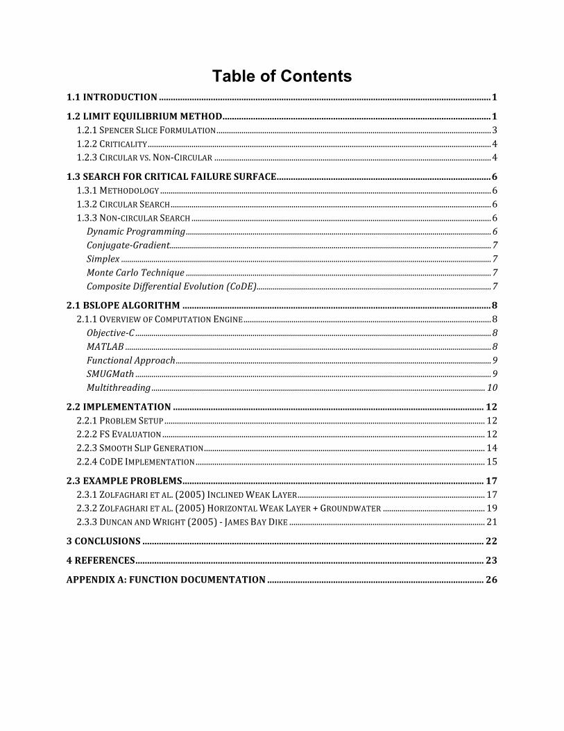
Table of Contents 1.1 INTRODUCTION ............................................................................................................................................. 1

1.2 LIMIT EQUILIBRIUM METHOD .................................................................................................................. 1 1.2.1 SPENCER SLICE FORMULATION .................................................................................................................................... 3 1.2.2 CRITICALITY ..................................................................................................................................................................... 4 1.2.3 CIRCULAR VS. NON-‐CIRCULAR ..................................................................................................................................... 4

1.3 SEARCH FOR CRITICAL FAILURE SURFACE ........................................................................................... 6 1.3.1 METHODOLOGY ............................................................................................................................................................... 6 1.3.2 CIRCULAR SEARCH .......................................................................................................................................................... 6 1.3.3 NON-‐CIRCULAR SEARCH ................................................................................................................................................ 6 Dynamic Programming ....................................................................................................................................................... 6 Conjugate-‐Gradient ............................................................................................................................................................... 7 Simplex ....................................................................................................................................................................................... 7 Monte Carlo Technique ....................................................................................................................................................... 7 Composite Differential Evolution (CoDE) .................................................................................................................... 7

2.1 BSLOPE ALGORITHM ................................................................................................................................... 8 2.1.1 OVERVIEW OF COMPUTATION ENGINE ....................................................................................................................... 8 Objective-‐C ................................................................................................................................................................................ 8 MATLAB ..................................................................................................................................................................................... 8 Functional Approach ............................................................................................................................................................ 9 SMUGMath ................................................................................................................................................................................ 9 Multithreading ..................................................................................................................................................................... 10

2.2 IMPLEMENTATION .................................................................................................................................... 12 2.2.1 PROBLEM SETUP .......................................................................................................................................................... 12 2.2.2 FS EVALUATION ........................................................................................................................................................... 12 2.2.3 SMOOTH SLIP GENERATION ....................................................................................................................................... 14 2.2.4 CODE IMPLEMENTATION ........................................................................................................................................... 15

2.3 EXAMPLE PROBLEMS ................................................................................................................................ 17 2.3.1 ZOLFAGHARI ET AL. (2005) INCLINED WEAK LAYER .......................................................................................... 17 2.3.2 ZOLFAGHARI ET AL. (2005) HORIZONTAL WEAK LAYER + GROUNDWATER ................................................. 19 2.3.3 DUNCAN AND WRIGHT (2005) -‐ JAMES BAY DIKE .............................................................................................. 21

3 CONCLUSIONS ................................................................................................................................................. 22

4 REFERENCES .................................................................................................................................................... 23

APPENDIX A: FUNCTION DOCUMENTATION ............................................................................................ 26

Acknowledgments The iOS implementation of the Limit Equilibrium algorithm used herein is based on a MATLAB code written by Mr. Mohammed Tabarroki of the University of Science of Malaysia. His advice and generosity in sharing his insights into the computational aspects of the implementation are gratefully acknowledged. Professor Stephen Wright pointed out an error in the May 2012 report, and we are grateful to him for his assistance. The James Bay test case has been updated with the results from our corrected, released version of the application.

1.1 Introduction The purpose of this project was to demonstrate the capabilities of mobile devices for advanced computation and analysis. bSLOPE, is a slope stability code adapted for iOS and for iPad using a new computational engine based on the work of Tabarroki (Tabarroki 2012), and Wang (2011). To this end the fundamentals of Limit Equilibrium slope stability analysis are reviewed first and then the computational algorithms are introduced as they are implemented in bSLOPE. This report has two objectives: (1) To acquaint the user with the process that is used in bSLOPE to analyze a particular slope in order to understand the internal structure of the algorithms and the limitations of the code; and (2) To give other researchers the information necessary to improve and extend bSLOPE’s open source computation engine. bSLOPE represents a new approach to slope stability analysis and engineering applications in general. Traditional slope stability packages contain proprietary, closed-source computation engines, and have limited user interfaces. These user interfaces often become the bottleneck in processing of slopes. bSLOPE uses innovative touch interfaces and drafting systems that take advantage of new technology in graphical interfaces. These interfaces allow the user of bSLOPE to rapidly formulate cross-sections and quickly perform the necessary analyses in the field. bSLOPE focuses on the most common tasks that an engineer would need to do in order to verify a slope’s safety. Its aim is to be simple and easy to use, while still using the most recent advances in numerical limit equilibrium algorithms. bSLOPE is not intended to be a replacement for many commercially accepted codes which have more analysis options. It is intended to complement these applications with a field component.

1.2 Limit Equilibrium Method The limit equilibrium method of analysis for static slopes is still the most widely used tool to analyze the stability of a given soil slope. It considers a soil continuum of different strata, and given a particular failure surface in the form of lines or arcs, a “Factor of Safety” is found through the application of force and/or moment equilibrium. The factor of safety is defined as the ratio of the resisting force or moment to the driving force or moment. So if a particular failure surface has a Factor of Safety (FS) of 1, then it is at the “limit” of equilibrium assumptions. A Factor of Safety less than 1 means that the driving forces are greater than the resisting forces and the slope will fail either in rotation, translation, or a combination thereof. In order to take an arbitrary geometry and automate the procedure of calculating a FS for a particular failure surface geometry, it is necessary to divide the sliding mass into sections. There are a variety of methods for performing this task; however, the most common method is to divide the mass into vertical slices. This is called the method of slices. The equilibrium

1

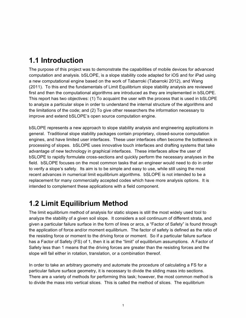
conditions are applied to each slice and contributions to either driving or resisting force or moment are computed. The sum of all driving and resisting moments and forces are then used to compute the overall Factor of Safety for the discretized sliding mass. Traditionally, the failure surfaces were defined as circular. This can be an accurate assumption in many homogenous soils; however, it is not true in most real world situations. Non-circular failure surfaces are much more likely in heterogeneous soils or where geological units form a complex geometry. There are several methods for computation of FS from a particular sliced sliding mass. Table 1, below, summarizes the methods most commonly used in practice and gives an overview of their use cases and assumptions. Method Limitations, Assumptions, and Equilibrium Conditions Satisfied Ordinary method of slices

(Fellenius 1927) Factors of safety low – very inaccurate for flat slopes with high pore pressures; only for circular

slip surfaces; assumes that normal force on the base of each slice is W cos α; one equation (moment equilibrium of entire mass), one unknown (factor of safety)

Bishop’s modified method (Bishop 1955)

Accurate method; only for circular slip surfaces; satisfies vertical equilibrium and overall moment equilibrium; assumes side forces on slices are horizontal; N+1 equations and unknowns

Force equilibrium methods

Satisfy force equilibrium; applicable to any shape of slip surface; assume side force inclinations, which may be the same for all slices or may vary from slice to slice; small side force inclinations result in values of F less than calculated using methods that satisfy all conditions of equilibrium; large inclinations result in values of F higher than calculated using methods that satisfy all conditions of equilibrium; 2N equations and unknowns

Janbu’s simplified method (Janbu 1968)

Force equilibrium method; applicable to any shape of slip surface; assumes side forces are horizontal (same for all slices); factors of safety are usually considerably lower than calculated using methods that satisfy all conditions of equilibrium; 2N equations and unknowns

Modified Swedish method (US Army Corps of Engineers 1970)

Force Equilibrium method, applicable to any shape of slip surface; assumes side force inclinations are equal to the inclination of the slope (same for all slices); factors of safety are often considerably higher than calculated using methods that satisfy all conditions of equilibrium; 2N equations and unknowns

Lowe and Karafiath’s method (Lowe and Karafiath 1960)

Generally most accurate of the force equilibrium methods; applicable to any shape of slip surface; assumes side force inclinations are average of slope surface and slip surface (varying from slice to slice); satisfies vertical and horizontal force equilibrium; 2N equations and unknowns

Janbu’s generalized procedure of slices (Janbu 1968)

Satisfies all conditions of equilibrium; applicable to any shape of slip surface; assumes heights of side forces above base of slice (varying from slice to slice); more frequent numerical convergence problems than some other methods; accurate method; 3N equations and unknowns

Spencer’s Method (Spencer 1967)

Satisfies all conditions of equilibrium; applicable to any shape of slip surface; assumes that inclinations of side forces are the same for every slice; side force inclination is calculated in the process of solution so that all conditions of equilibrium are satisfied; accurate method; 3N equations and unknowns

Morgensertn and Price’s method (Morgenstern and Price 1965)

Satisfies all conditions of equilibrium; applicable to any shape of slip surface; assumes that inclinations of side forces follow prescribed pattern, called f(x); side force inclinations can be the same or can vary from slice to slice; side force inclinations are calculated in the process of solution so that all conditions of equilibrium are satisfied; accurate method; 3N equations and unknowns

Sarma’s method (Sarma 1973)

Satisfies all conditions of equilibrium; applicable to any shape of slip surface; assumes that magnitudes of vertical side forces follow prescribed patterns; calculates horizontal acceleration for barely stable equilibrium; by prefactoring strengths and iterating to find the value of the prefactor that results in zero horizontal acceleration for barely stable equilibrium, the value of the conventional factor of safety can be determined; 3N equations, 3N unknowns.

Table 1: List of FS evaluation methods, after Duncan (1996)

2

Most methods of computing the FS for a failure surface can be calculated through a common formulation published by Fredlund and Krahn (1977) called the General Limit Equilibrium method (GLE). The GLE encompasses the Simplified Bishop, Spencer’s, Janbu’s simplified, Janbu’s rigorous, and the Morgenstern-Price methods. This approach is used in bSLOPE as the basis for its FS calculations. This allows bSLOPE to rapidly compute the FS value for many different methods using essentially the same algorithm.

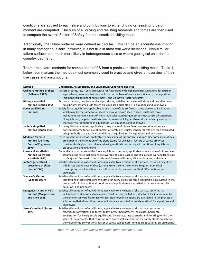
1.2.1 Spencer Slice Formulation In order to understand how the algorithm works, we must first understand how the FS computation is executed within the algorithm.

Fig. 1. Forces acting for the method of slices applied to a composite sliding surface. After Fredlund and Krahn (1977) The algorithm specifies the variables associated with each slice using the following notation. bSLOPE parameter names follow in blue according to Tabarroki’s (Tabarroki 2012) original naming scheme. 𝑊 = Total weight of the slice of width b and height h. (sliceWeight) 𝑃 = Total normal force on the base of the slice over a length l. (sliceNm and sliceNf for

moment and force equilibrium, respectively) 𝑆! = Shear force mobilized on the base of the slice. It is a percentage of the shear strength

as defined by the Mohr-Coulomb equation. That is, 𝑆! = 𝑙 {𝑐! + !!− 𝑢 tan𝜙!}/𝐹𝑆

where 𝑐! = effective cohesion parameter, 𝜙! = effective angle of internal friction, 𝐹𝑆 = factor of safety, and 𝑢 = pore-water pressure.

𝑅 = Radius or the moment arm associated with the mobilized shear force 𝑆!. (sliceR) 𝑓 = Perpendicular offset of the normal force from the center of rotation. (slicef)

3

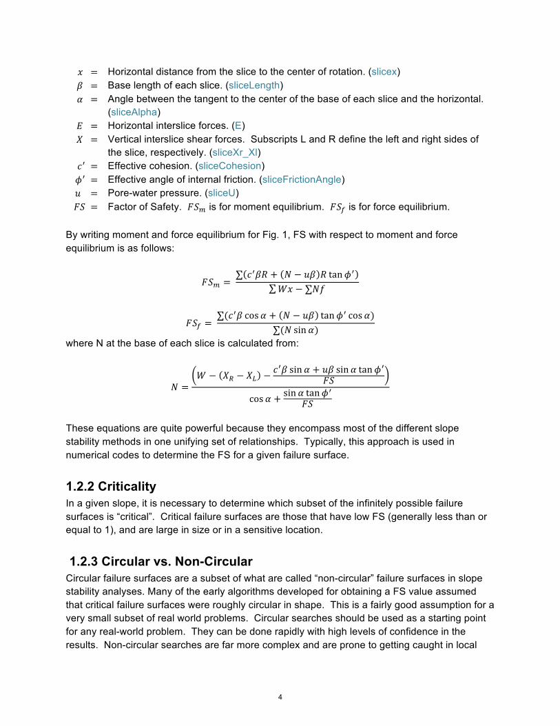
𝑥 = Horizontal distance from the slice to the center of rotation. (slicex) 𝛽 = Base length of each slice. (sliceLength) 𝛼 = Angle between the tangent to the center of the base of each slice and the horizontal.

(sliceAlpha) 𝐸 = Horizontal interslice forces. (E) 𝑋 = Vertical interslice shear forces. Subscripts L and R define the left and right sides of

the slice, respectively. (sliceXr_Xl) 𝑐! = Effective cohesion. (sliceCohesion) 𝜙! = Effective angle of internal friction. (sliceFrictionAngle) 𝑢 = Pore-water pressure. (sliceU) 𝐹𝑆 = Factor of Safety. 𝐹𝑆! is for moment equilibrium. 𝐹𝑆! is for force equilibrium.

By writing moment and force equilibrium for Fig. 1, FS with respect to moment and force equilibrium is as follows:

𝐹𝑆! = ∑ 𝑐!𝛽𝑅 + 𝑁 − 𝑢𝛽 𝑅 tan𝜙!

𝑊𝑥 − ∑𝑁𝑓

𝐹𝑆! = ∑(𝑐!𝛽 cos𝛼 + 𝑁 − 𝑢𝛽 tan𝜙! cos𝛼)

∑(𝑁 sin 𝛼)

where N at the base of each slice is calculated from:

𝑁 =𝑊 − 𝑋! − 𝑋! − 𝑐

!𝛽 sin 𝛼 + 𝑢𝛽 sin 𝛼 tan𝜙!𝐹𝑆

cos𝛼 + sin 𝛼 tan𝜙!

𝐹𝑆

These equations are quite powerful because they encompass most of the different slope stability methods in one unifying set of relationships. Typically, this approach is used in numerical codes to determine the FS for a given failure surface.

1.2.2 Criticality In a given slope, it is necessary to determine which subset of the infinitely possible failure surfaces is “critical”. Critical failure surfaces are those that have low FS (generally less than or equal to 1), and are large in size or in a sensitive location.

1.2.3 Circular vs. Non-Circular Circular failure surfaces are a subset of what are called “non-circular” failure surfaces in slope stability analyses. Many of the early algorithms developed for obtaining a FS value assumed that critical failure surfaces were roughly circular in shape. This is a fairly good assumption for a very small subset of real world problems. Circular searches should be used as a starting point for any real-world problem. They can be done rapidly with high levels of confidence in the results. Non-circular searches are far more complex and are prone to getting caught in local

4

minima. Therefore, non-circular searches should be attempted very carefully. The geometry of the problem may prevent convergence. Engineering judgment is required in selecting entry or exit regions that will guide the slip surface to areas that are believed to be most susceptible to failure.

5

1.3 Search for Critical Failure Surface

1.3.1 Methodology In general, the search for the critical failure surface in a given slope is a problem of minimization. In slope stability analysis, we are attempting to find the failure surface with the minimum FS that is also meaningful in the real-world context. We do not want the search to get caught on infinitesimally small failures, or generate kinematically inadmissible slip surfaces. The objective function in this case is the GLE, the inputs are the X and Y coordinates of the slip surfaces, and the output is the FS. By intelligently analyzing the output of the objective function after each iteration, it is possible to modify the inputs (in this case, the slip surface) to attempt to attain a lower-FS failure surface.

1.3.2 Circular Search If the failure surface is limited to circular geometry then the optimization problem becomes very simple. We must only consider center, radii, and the boundaries of the slope. This process has been implemented in many codes as a “grid-and-radius” search in which the user specifies a grid of centers and a range of radii to test. The FS values from the permutations of these two parameters are computed, and the lowest value of FS is assumed to be from the critical surface. A “heat map” of FS can then be generated. bSLOPE implements a very simple evolutionary algorithm that varies three parameters to locate the minimum, entry and exit location, and the radius of the circle.

1.3.3 Non-circular Search If failure surfaces are not constrained to be circular, then the search for criticality becomes much more complex. Traditionally, engineers would have to use their experience to define several predicted non-circular failure modes based on the geology of the slope. These would be input into the computer application, which would then calculate the FS for these special cases. This limited search requires a great deal of work and a trial-and-error approach, which can easily lead to problems if important failure surfaces are not considered. The task of the non-circular search algorithm therefore is to find the critical, kinematically admissible failure surface within a user-defined region. There are many approaches to this problem. The first algorithms developed were deterministic in nature however they have become highly complex to deal with the many different types of failures and situations. Other search algorithms have been developed based on advanced evolutionary or statistical methods that automatically optimize to the correct solution. These methods have the benefit of being easy to understand in theory, and if managed properly, can match deterministic approaches to the problem in both speed and accuracy.

6

Dynamic Programming Bellman (1957) originally created a mathematical minimization technique called dynamic programming. The algorithm was first applied to slope stability by Baker in 1980. The method is very complex compared to many of the other optimization methods, and requires many more parameters to be specified for the soil strata, such as Poisson’s ratio and elastic modulus. This introduces additional uncertainty in the results, and this method has not been used widely since its introduction.

Conjugate-Gradient Arai and Tagyo (1985) used the conjugate gradient method, which is probably the most prominent method of solving sparse systems of linear equations. It is often used in finite element codes, and works well here, though more efficient algorithms have been proposed.

Simplex A simplex is a geometrical figure in a N-dimensional space consisting of N+1 vertices and all their interconnecting line segments (Bardet and Kapuskar 1989). In the case of the N-dimensional slip surface with N+1 vertices, the simplex is used along with reflection, reflection plus expansion, local contraction, and global contraction to generate successively lower FS simplex geometries.

Monte Carlo Technique Monte Carlo minimization techniques operate through random search for a function with several variables. The first implementations of this technique in the slope stability context were inefficient and required a tremendous number of iterations before the critical failure surface could be found. To address this constraint, Greco (1996) presented the first “random walk” Monte Carlo method. Through intelligent generation of kinematically admissible slip surfaces for each iteration of the algorithm, Greco’s algorithm is comparable in speed to many deterministic algorithms.

Composite Differential Evolution (CoDE) This method was proposed as a general optimization algorithm by Wang (2011). It is a highly efficient variant of the Differential Evolution process whereby an initial population is modified through mutation, crossover, and selection to produce succeeding generations closer to the global optimum. This general optimization algorithm was competitive with other general methods (Wang 2011). Tabarroki (Tabarroki 2012) used MATLAB to implement a version of this optimization technique for the X and Y coordinates of the non-circular slip surface and was able to create the high-performance solution that is implemented in bSLOPE.

7

2.1 bSLOPE Algorithm

2.1.1 Overview of Computation Engine The computation engine for bSLOPE was ported from an implementation of the Composite Differential Evolution algorithm originally written by Tabarroki (Tabarroki 2012). The majority of the work in the creation of bSLOPE was in translating and optimizing this MATLAB code to the high-level native programming language Objective-C. Through extensive memory analysis and refactoring many of the individual functions to utilize modern multi-cored discrete graphics and CPUs, bSLOPE has been able to attain a 5-10x increase in speed over the MATLAB implementation on the same hardware. A major problem for the industry has been the closed-source nature of the existing computation platforms. Codes like SLOPE/W (Geo-Slope 2001) use methods of analysis that are well-established and rigorously defined, yet they are closed-source and proprietary, which means that their improvement and optimization for the entire industry depends on the authors of the code only. Consequently, slope stability research routinely entails either “reinventing the wheel” by writing a limit equilibrium code from scratch, or using an outdated core written in the 70’s. bSLOPE’s open computational engine will be available for all researchers to use and extend moving forward.

Objective-C Objective-C is a relatively widely used language that has many advantages for high-speed scientific computing on limited resources. It is a superset of the low-level C language, which means that anything written in C will also run in Objective-C. Objective-C however also has high-level Object-oriented systems in place which give it great flexibility in its memory management. Its primary advantage over other high-level languages such as Ruby or Java is its memory management and speed. Objective-C is a compiled language, which means that the resulting compiled binary package runs directly on the processor of the system without an interpreter or virtual machine layer between the program and the hardware. This allows it to use intelligent memory allocations and modifiers within objective wrappers without the heavy overhead of automatic “garbage” disposal in Ruby or Java. C++ is another logical choice for bSLOPE; however, its unintuitive syntax would be challenging for many researchers to use, especially if they are used to MATLAB. Objective-C uses similar syntax to many other high-level programming languages such as Ruby or Java, and contains many of the niceties of recent advancements in computer science.

MATLAB MATLAB is an interpreted language with dynamic, inferenced types. It is a high-level language with nice syntax for performing matrix operations, and has many high-performance matrix math libraries built-in. However, when building a large custom code, it has limitations. The interpreter

8

is quite good at optimizing matrix computations, but can never be as fast as a compiled code due to the large overhead associated with the interpretation layer and garbage collector. The interpretation layer of MATLAB also has problems with I/O operations to memory buffers where its variables are stored. These I/O operations often take much more time than the actual computations do. C allows the user to pass variables as pointers to locations in memory and does not necessitate the duplication of that memory to work on a particular variable. MATLAB also uses high-precision computing for many of its core libraries, which makes computations much slower than single floating-point precision calculations. In rewriting the code, C float (single precision) primitives were used which are more than accurate enough for slope stability calculations. C floats retain accuracy out to about the 6th decimal place, which is sufficient for our purposes. The primary challenge in translating the code from MATLAB was replicating the functionality of many of MATLAB’s built-in vector and matrix math functions. Custom implementations for these functions were written in Obj-C.

Functional Approach There are many application structure paradigms that can be implemented to make a body of code more easily understandable and maintainable. The two primary approaches currently popular are Object Oriented applications and functional applications. Of course, most real-world applications are a mix of the two, they generally fall somewhere on the spectrum closer to one side or the other. bSLOPE’s computation engine was built with a functional approach. This means that the stages of computation are broken up into functional components and these components have strict rules for input and output. Generally, functions with pointer arguments will not modify the memory of parent functions and they will allocate and free their own workspaces in memory. This has many benefits from a research perspective. Each individual function can be replaced without destroying the functionality of the entire application, and refactoring becomes much simpler. Performance enhancements from minute changes in particular functions can be measured and calibrated simply. Of course, there are many object-oriented parts of bSLOPE as well, starting with its math library which uses objects to represent abstract data types. Objective-C has a great facility for easing the use of either application paradigm.

SMUGMath The SMUGMath library was used as a base and heavily extended to mimic these functionalities in Objective-C. At the basis of this library is the RealVector class. This class acts as an Objective-C wrapper for a C float array. They allow C float arrays to be created and destroyed through retain counting. RealVectors use the virtual Digital Signals Processing library from Apple (vDSP) to perform in-place mathematical transformations on floats. This reduces memory duplication and allows bSLOPE to use the multicored discrete graphics chips in Apple’s devices.

9

For matrix operations, bSLOPE uses the RealMatrix class to represent the matrix data. A RealMatrix is a wrapper for a RealVector with a specific mapping from elements in the 2D matrix to specific elements in the vector. Processor intensive matrix operations like sorting and searching are done with the vDSP library, which has highly optimized implementations.

Multithreading MATLAB has some great multithreading tools that make it incredibly simple to implement a parallel algorithm for multi-core processors. Tabarroki (Tabarroki 2012) used the “parfor” function to parallelize FS evaluations for each stage of the evolutionary algorithm. There is no simple way to duplicate this functionality in Objective-C. The performance gains associated with splitting individual threads is often elusive if not done in the proper way. The overhead associated with creating and running a new thread is not small. Also, deciding the optimal number and execution order of threads to ensure that resources are not wasted and performance is negatively impacted is difficult. Objective C as implemented in iOS provides a multithreading library that is not quite as simple as the “parfor” command in MATLAB. It is called Grand Central Dispatch, and optimizes the execution order and number of concurrent processes for the current memory and processor demands. It creates and manages C threads, and allows applications to queue code in the form of Objective-C “blocks”. Blocks are compiled pieces of code that are similar to standard C functions, but can be passed as part of other functions’ variable scope at runtime. Grand Central Dispatch manages queues of blocks that are executed on the correct number of threads for the current runtime environment to assure the fastest execution. bSLOPE mimics the “parfor” functionality by queuing blocks that evaluate each individual FS evaluation. These blocks then queue completion blocks on the main thread that insert their results into a synchronous data source held in a singleton data object. Once all FS evaluation blocks have been processed, the last item in the queue begins the next stage of post-processing these FS and trial vector selection. Thread safety is one of the biggest challenges faced by creators of multithreaded code. The functional approach to bSLOPE makes this issue relatively simple to deal with. Each function is passed its object parameters as pointers to locations in memory where the objects are located and all primitives are passed as values. Functions are not allowed to modify the objects passed in and are responsible for allocating and freeing the memory required to perform their operations. The only operation that is not thread-safe by default is the access to the passed in objects. This is solved by placing @synchronized blocks around the accessors, which requires successive requests to wait in a queue in order to read the memory. Most of the mobile processors that bSLOPE is designed for are single-core ARM chips, and so are not able to see any performance gains by implementing this code. In fact, this approach will tremendously slow down the code because of the management overhead associated with the creation and destruction of thread processes and memory spaces. The third-generation iPad does have a dual core A5X chip, but in our testing the performance gains from multithreading

10

the code on this small processor were nonexistent. By default, bSLOPE’s computation engine has this section of code disabled until quad-core CPUs are introduced for iPad. Although multithreaded computation is disabled for the CPU, discrete graphics chips are used for the vector computation when present in the device. In the third-generation iPad, a quad-core discrete graphics chip is in place that performs matrix math at high speed through Apple’s vDSP library. This allows dramatic increases in speed when compared to the same computations on the CPU.

11

2.2 Implementation

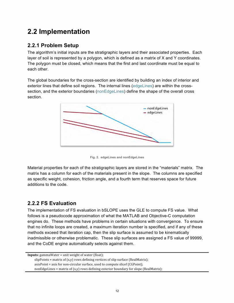
2.2.1 Problem Setup The algorithm’s initial inputs are the stratigraphic layers and their associated properties. Each layer of soil is represented by a polygon, which is defined as a matrix of X and Y coordinates. The polygon must be closed, which means that the first and last coordinate must be equal to each other. The global boundaries for the cross-section are identified by building an index of interior and exterior lines that define soil regions. The internal lines (edgeLines) are within the cross-section, and the exterior boundaries (nonEdgeLines) define the shape of the overall cross section.

Fig. 2. edgeLines and nonEdgeLines

Material properties for each of the stratigraphic layers are stored in the “materials” matrix. The matrix has a column for each of the materials present in the slope. The columns are specified as specific weight, cohesion, friction angle, and a fourth term that reserves space for future additions to the code.

2.2.2 FS Evaluation The implementation of FS evaluation in bSLOPE uses the GLE to compute FS value. What follows is a pseudocode approximation of what the MATLAB and Objective-C computation engines do. These methods have problems in certain situations with convergence. To ensure that no infinite loops are created, a maximum iteration number is specified, and if any of these methods exceed that iteration cap, then the slip surface is assumed to be kinematically inadmissible or otherwise problematic. These slip surfaces are assigned a FS value of 99999, and the CoDE engine automatically selects against them. Inputs: gammaWater = unit weight of water (float);

slipPoints = matrix of (x,y) rows defining vertices of slip surface (RealMatrix); axisPoint = axis for non-‐circular surface, used to compute slicef (CGPoint); nonEdgeLines = matrix of (x,y) rows defining exterior boundary for slope (RealMatrix);

12

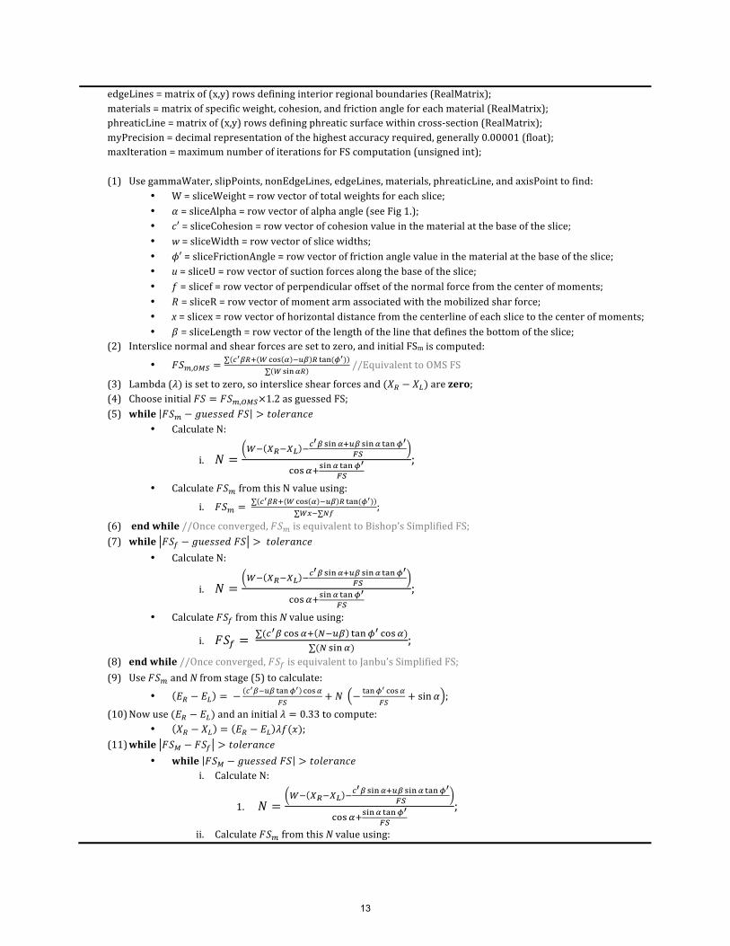
edgeLines = matrix of (x,y) rows defining interior regional boundaries (RealMatrix); materials = matrix of specific weight, cohesion, and friction angle for each material (RealMatrix); phreaticLine = matrix of (x,y) rows defining phreatic surface within cross-‐section (RealMatrix); myPrecision = decimal representation of the highest accuracy required, generally 0.00001 (float); maxIteration = maximum number of iterations for FS computation (unsigned int); (1) Use gammaWater, slipPoints, nonEdgeLines, edgeLines, materials, phreaticLine, and axisPoint to find:

• W = sliceWeight = row vector of total weights for each slice; • 𝛼 = sliceAlpha = row vector of alpha angle (see Fig 1.); • 𝑐′ = sliceCohesion = row vector of cohesion value in the material at the base of the slice; • w = sliceWidth = row vector of slice widths; • 𝜙′ = sliceFrictionAngle = row vector of friction angle value in the material at the base of the slice; • u = sliceU = row vector of suction forces along the base of the slice; • 𝑓 = slicef = row vector of perpendicular offset of the normal force from the center of moments; • 𝑅 = sliceR = row vector of moment arm associated with the mobilized shar force; • x = slicex = row vector of horizontal distance from the centerline of each slice to the center of moments; • 𝛽 = sliceLength = row vector of the length of the line that defines the bottom of the slice;

(2) Interslice normal and shear forces are set to zero, and initial FSm is computed:

• 𝐹𝑆!,!"# =∑ !!!"! ! !"# ! !!" ! !"#(!!)

∑ ! !"#!" //Equivalent to OMS FS

(3) Lambda (𝜆) is set to zero, so interslice shear forces and (𝑋! − 𝑋!) are zero; (4) Choose initial 𝐹𝑆 = 𝐹𝑆!,!"#×1.2 as guessed FS; (5) while 𝐹𝑆! − 𝑔𝑢𝑒𝑠𝑠𝑒𝑑 𝐹𝑆 > 𝑡𝑜𝑙𝑒𝑟𝑎𝑛𝑐𝑒

• Calculate N:

i. 𝑁 =!! !!!!! !!

!! !"#!!!" !"#! !"#!!

!"

!"#!!!"#! !"#!!

!"

;

• Calculate 𝐹𝑆! from this N value using:

i. 𝐹𝑆! = ∑ !!!"! ! !"# ! !!" ! !"#(!!)∑!"!∑!"

;

(6) end while //Once converged, 𝐹𝑆! is equivalent to Bishop’s Simplified FS; (7) while 𝐹𝑆! − 𝑔𝑢𝑒𝑠𝑠𝑒𝑑 𝐹𝑆 > 𝑡𝑜𝑙𝑒𝑟𝑎𝑛𝑐𝑒

• Calculate N:

i. 𝑁 =!! !!!!! !!

!! !"#!!!" !"#! !"#!!

!"

!"#!!!"#! !"#!!

!"

;

• Calculate 𝐹𝑆! from this N value using:

i. 𝐹𝑆! = ∑(!!! !"#!! !!!" !"#!! !"#!)

∑(! !"#!);

(8) end while //Once converged, 𝐹𝑆! is equivalent to Janbu’s Simplified FS; (9) Use 𝐹𝑆! and N from stage (5) to calculate:

• 𝐸! − 𝐸! = − !!!!!" !"#!! !"#!!"

+ 𝑁 − !"#!! !"#!!"

+ sin𝛼 ;

(10) Now use (𝐸! − 𝐸!) and an initial 𝜆 = 0.33 to compute: • 𝑋! − 𝑋! = 𝐸! − 𝐸! 𝜆𝑓(𝑥);

(11) while 𝐹𝑆! − 𝐹𝑆! > 𝑡𝑜𝑙𝑒𝑟𝑎𝑛𝑐𝑒 • while 𝐹𝑆! − 𝑔𝑢𝑒𝑠𝑠𝑒𝑑 𝐹𝑆 > 𝑡𝑜𝑙𝑒𝑟𝑎𝑛𝑐𝑒

i. Calculate N:

1. 𝑁 =!! !!!!! !!

!! !"#!!!" !"#! !"#!!

!"

!"#!!!"#! !"#!!

!"

;

ii. Calculate 𝐹𝑆! from this N value using:

13

1. 𝐹𝑆! = ∑ !!!"! ! !"# ! !!" ! !"#(!!)∑!"!∑!"

;

• end while • while 𝐹𝑆! − 𝑔𝑢𝑒𝑠𝑠𝑒𝑑 𝐹𝑆 > 𝑡𝑜𝑙𝑒𝑟𝑎𝑛𝑐𝑒

i. Calculate N:

1. 𝑁 =!! !!!!! !!

!! !"#!!!" !"#! !"#!!

!"

!"#!!!"#! !"#!!

!"

;

ii. Calculate 𝐹𝑆! from this N value using:

1. 𝐹𝑆! = ∑(!!! !"#!! !!!" !"#!! !"#!)

∑(! !"#!);

• end while • Use 𝐹𝑆! and N from stage (5) to calculate:

i. 𝐸! − 𝐸! = − !!!!!" !"#!! !"#!!"

+ 𝑁 − !"#!! !"#!!"

+ sin𝛼 ;

• Use Newton-‐Raphson method to compute 𝜆. Use this and (𝐸! − 𝐸!) to compute: i. 𝑋! − 𝑋! = 𝐸! − 𝐸! 𝜆𝑓(𝑥);

(12) end while //Once converged, the joint FS value here is equal to either the Morgenstern-‐Price or the Spencer’s FS value depending on the function 𝑓(𝑥);

Output: FS value for the given slip surface;

Fig. 3. Pseudocode for FS evaluation

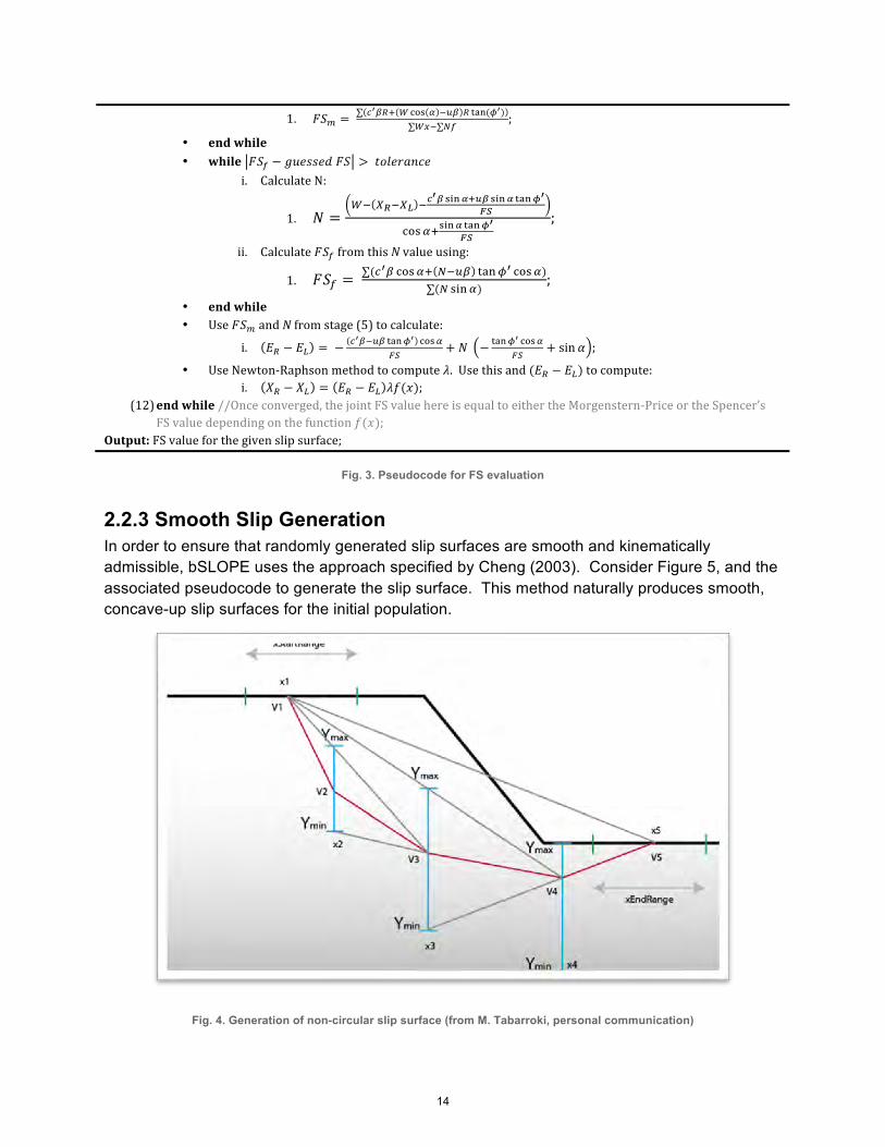
2.2.3 Smooth Slip Generation In order to ensure that randomly generated slip surfaces are smooth and kinematically admissible, bSLOPE uses the approach specified by Cheng (2003). Consider Figure 5, and the associated pseudocode to generate the slip surface. This method naturally produces smooth, concave-up slip surfaces for the initial population.

Fig. 4. Generation of non-circular slip surface (from M. Tabarroki, personal communication)

14

Input: ground = matrix representation of path defining the ground surface – composed of (x,y) row vectors;

bedrock = matrix representation of path defining “bedrock”, a lower boundary for our search – composed of (x,y) row vectors;

xStartRange = row vector with an upper and lower X bound for the start range of the slip in the ground surface;

xEndRange = row vector with upper and lower X bound for the end range of the slip in the ground surface;

(1) Generate a random 𝑥! and 𝑥! within the xStartRange and xEndRange, respectively; (2) Generate 𝑥! through 𝑥!!! by uniformly dividing the horizontal distance between 𝑥! and 𝑥!; (3) 𝑌!"# and 𝑌!"# are calculated for 𝑥!!!; (4) 𝜎!!! is randomly generated between 0 and 1; (5) 𝑦!!! = 𝜎!!! 𝑌!"# − 𝑌!"# + 𝑌!"# ; (6) Steps 3-‐5 are repeated for each successive x-‐coordinate back towards 𝑥!;

Output: matrix of [𝑥!, 𝑥!,𝜎!,… 𝜎!!!] defining the slip;

[G = generation number; FES = number of function evaluations; F & Cr = control parameter settings]

Fig. 5. Pseudocode of general CoDE Algorithm (from Wang et al. 2011)

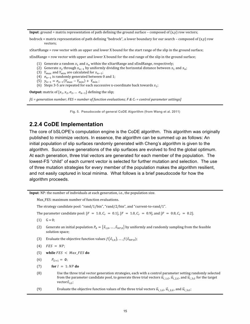
2.2.4 CoDE Implementation The core of bSLOPE’s computation engine is the CoDE algorithm. This algorithm was originally published to minimize vectors. In essence, the algorithm can be summed up as follows: An initial population of slip surfaces randomly generated with Cheng’s algorithm is given to the algorithm. Successive generations of the slip surfaces are evolved to find the global optimum. At each generation, three trial vectors are generated for each member of the population. The lowest-FS “child” of each current vector is selected for further mutation and selection. The use of three mutation strategies for every member of the population makes the algorithm resilient, and not easily captured in local minima. What follows is a brief pseudocode for how the algorithm proceeds.

Input: NP: the number of individuals at each generation, i.e., the population size.

Max_FES: maximum number of function evaluations.

The strategy candidate pool: “rand/1/bin”, “rand/2/bin”, and “current-‐to-‐rand/1”.

The parameter candidate pool: [𝐹 = 1.0,𝐶! = 0.1], [𝐹 = 1.0,𝐶! = 0.9], and [𝐹 = 0.8,𝐶! = 0.2].

(1) G = 0;

(2) Generate an initial population 𝑃! = 𝑥!,!,… , 𝑥!",! by uniformly and randomly sampling from the feasible solution space;

(3) Evaluate the objective function values 𝑓 𝑥!,! ,… , 𝑓(𝑥!",!);

(4) 𝐹𝐸𝑆 = 𝑁𝑃;

(5) while 𝐹𝐸𝑆 < 𝑀𝑎𝑥_𝐹𝐸𝑆 do

(6) 𝑃!!! = ∅;

(7) for 𝐼 = 1:𝑁𝑃 do

(8) Use the three trial vector generation strategies, each with a control parameter setting randomly selected from the parameter candidate pool, to generate three trial vectors 𝑢!_!,! , 𝑢!_!,! , and 𝑢!_!,! for the target vector𝑥!,!;

(9) Evaluate the objective function values of the three trial vectors 𝑢!_!,! , 𝑢!_!,! , and 𝑢!_!,!;

15

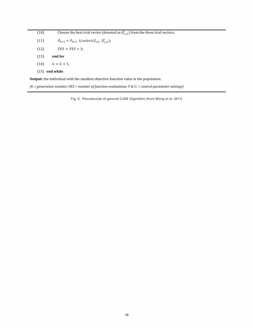
(10) Choose the best trial vector (denoted as 𝑢!!,!∗ ) from the three trial vectors;

(11) 𝑃!!! = 𝑃!!! 𝑠𝑒𝑙𝑒𝑐𝑡(𝑥!,! , 𝑢!!,!∗ );

(12) 𝐹𝐸𝑆 = 𝐹𝐸𝑆 + 3;

(13) end for

(14) 𝐺 = 𝐺 + 1;

(15) end while

Output: the individual with the smallest objective function value in the population.

[G = generation number; FES = number of function evaluations; F & Cr = control parameter settings]

Fig. 6. Pseudocode of general CoDE Algorithm (from Wang et al. 2011)

16

2.3 Example Problems

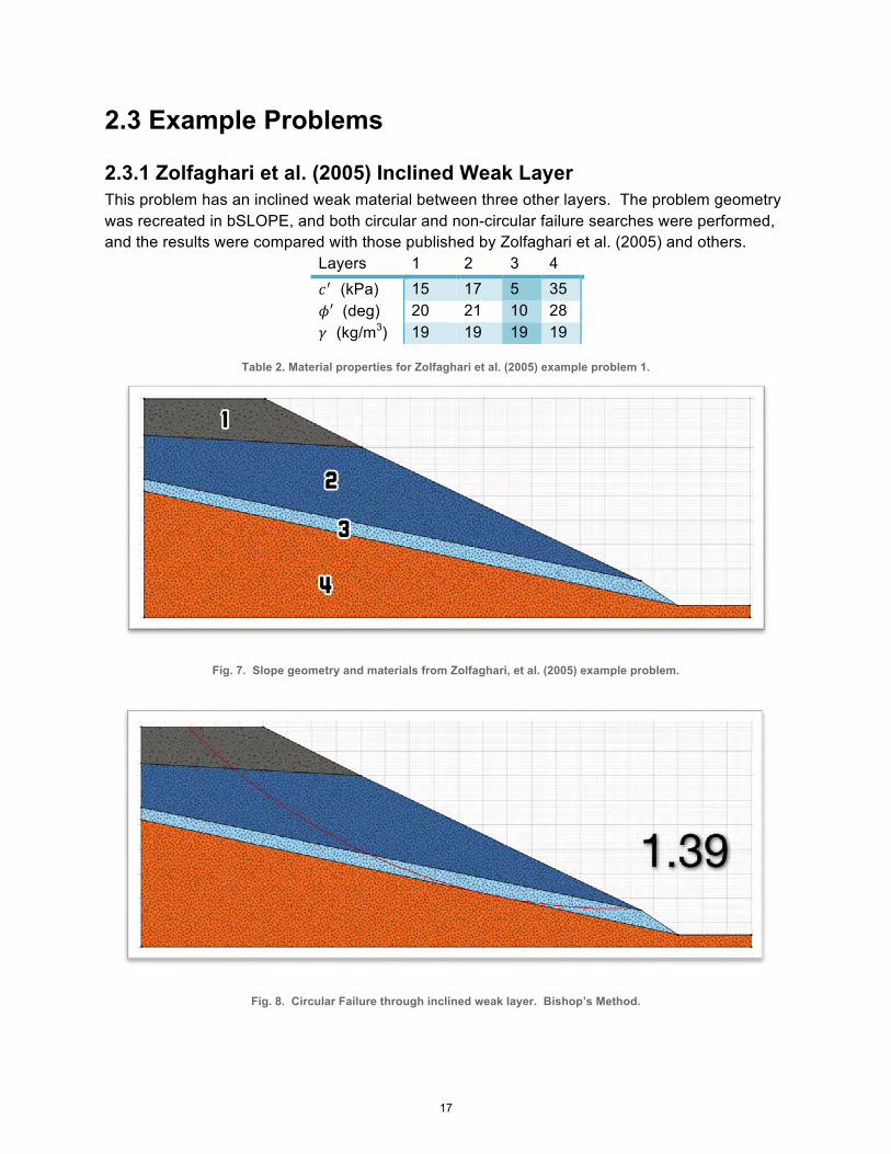
2.3.1 Zolfaghari et al. (2005) Inclined Weak Layer This problem has an inclined weak material between three other layers. The problem geometry was recreated in bSLOPE, and both circular and non-circular failure searches were performed, and the results were compared with those published by Zolfaghari et al. (2005) and others.

Layers 1 2 3 4 𝑐! (kPa) 15 17 5 35 𝜙′ (deg) 20 21 10 28 𝛾 (kg/m3) 19 19 19 19

Table 2. Material properties for Zolfaghari et al. (2005) example problem 1.

Fig. 7. Slope geometry and materials from Zolfaghari, et al. (2005) example problem.

Fig. 8. Circular Failure through inclined weak layer. Bishop’s Method.

17

Search Method FS Value Simple Genetic Algorithm (Zolfaghari et al. 2005),

Bishop 1.475

CoDE (Tabarroki 2012, this report), Bishop 1.39

Table 3. FS values from circular failure in Example Problem 1.

The FS values for the circular failure analysis are very close, and the CoDE engine produced a slip surface that is nearly identical to the results in Zolfaghari et al. (2005). bSLOPE produces a FS that is 5.7% less than the reference value.

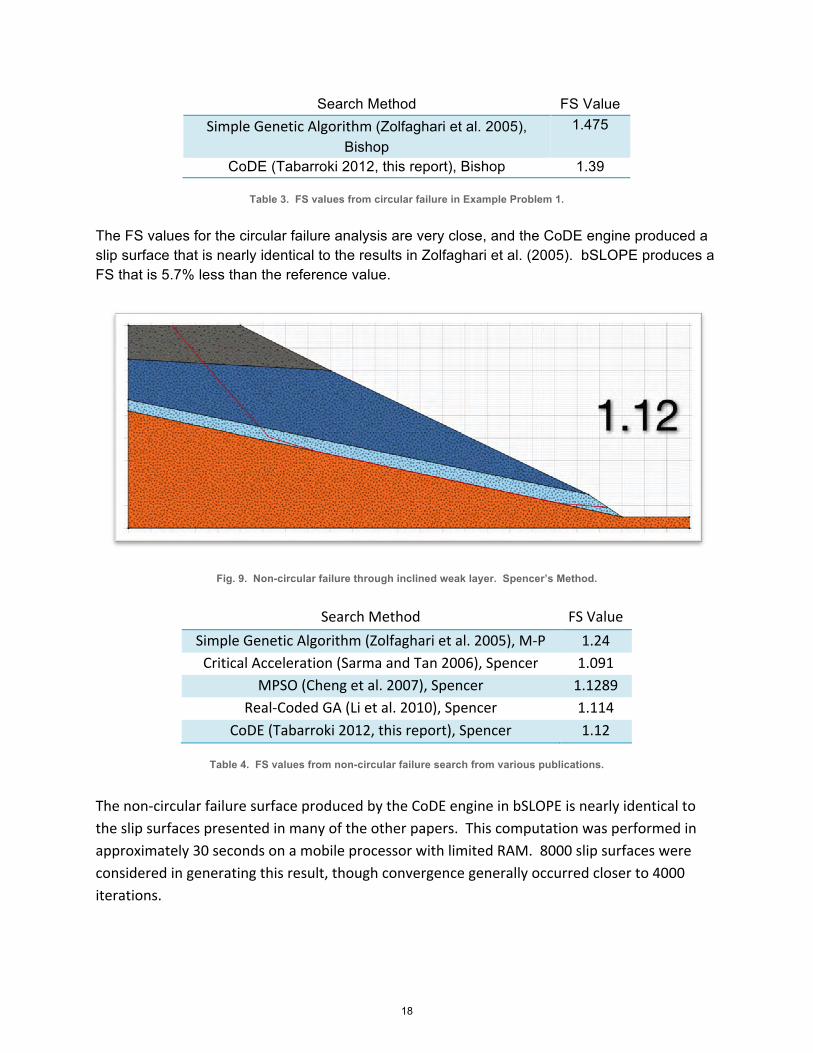
Fig. 9. Non-circular failure through inclined weak layer. Spencer’s Method.

Search Method FS Value

Simple Genetic Algorithm (Zolfaghari et al. 2005), M-‐P 1.24 Critical Acceleration (Sarma and Tan 2006), Spencer 1.091

MPSO (Cheng et al. 2007), Spencer 1.1289 Real-‐Coded GA (Li et al. 2010), Spencer 1.114

CoDE (Tabarroki 2012, this report), Spencer 1.12

Table 4. FS values from non-circular failure search from various publications.

The non-‐circular failure surface produced by the CoDE engine in bSLOPE is nearly identical to the slip surfaces presented in many of the other papers. This computation was performed in approximately 30 seconds on a mobile processor with limited RAM. 8000 slip surfaces were considered in generating this result, though convergence generally occurred closer to 4000 iterations.

18

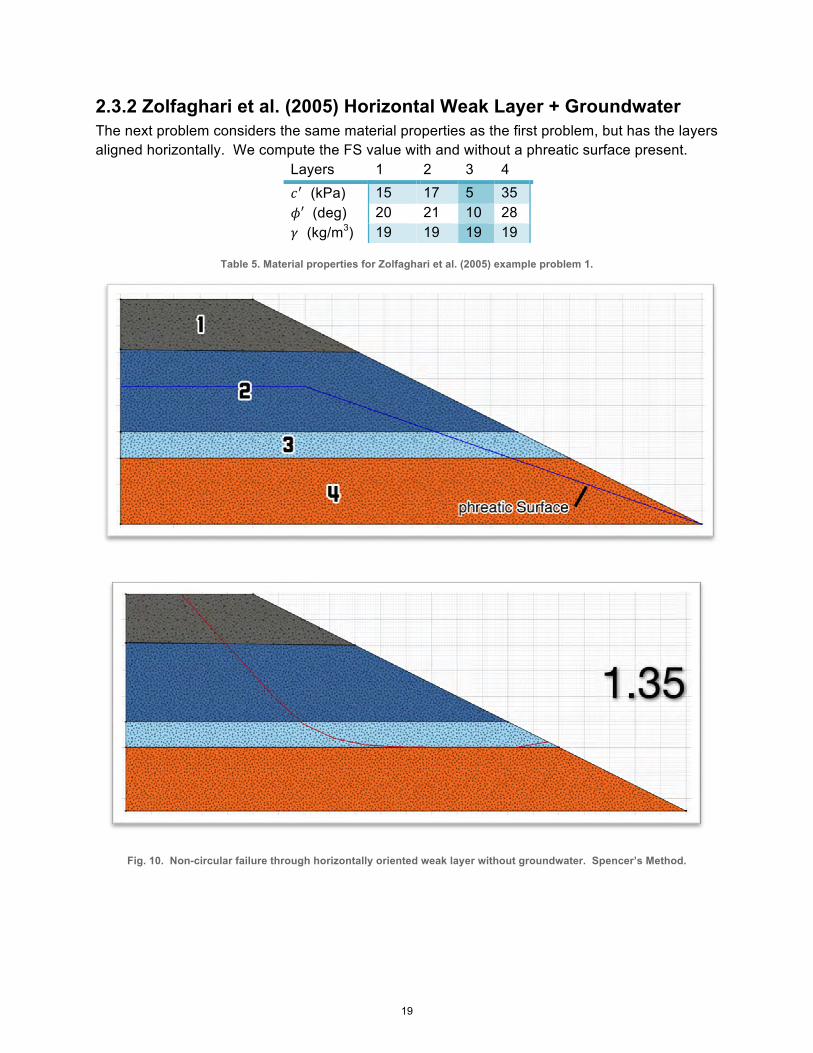
2.3.2 Zolfaghari et al. (2005) Horizontal Weak Layer + Groundwater The next problem considers the same material properties as the first problem, but has the layers aligned horizontally. We compute the FS value with and without a phreatic surface present.

Layers 1 2 3 4 𝑐! (kPa) 15 17 5 35 𝜙′ (deg) 20 21 10 28 𝛾 (kg/m3) 19 19 19 19

Table 5. Material properties for Zolfaghari et al. (2005) example problem 1.

Fig. 10. Non-circular failure through horizontally oriented weak layer without groundwater. Spencer’s Method.

19

Search Method FS Value Simple Genetic Algorithm (Zolfaghari et al. 2005), M-‐P 1.48 Simulated Annealing (Cheng and Lau 2008), Spencer 1.3961 Genetic Algorithm (Cheng and Lau 2008), Spencer 1.3733

Simple Harmony Search (Cheng and Lau 2008), Spencer 1.3729 Modified Harmony Search (Cheng and Lau 2008), Spencer 1.3501


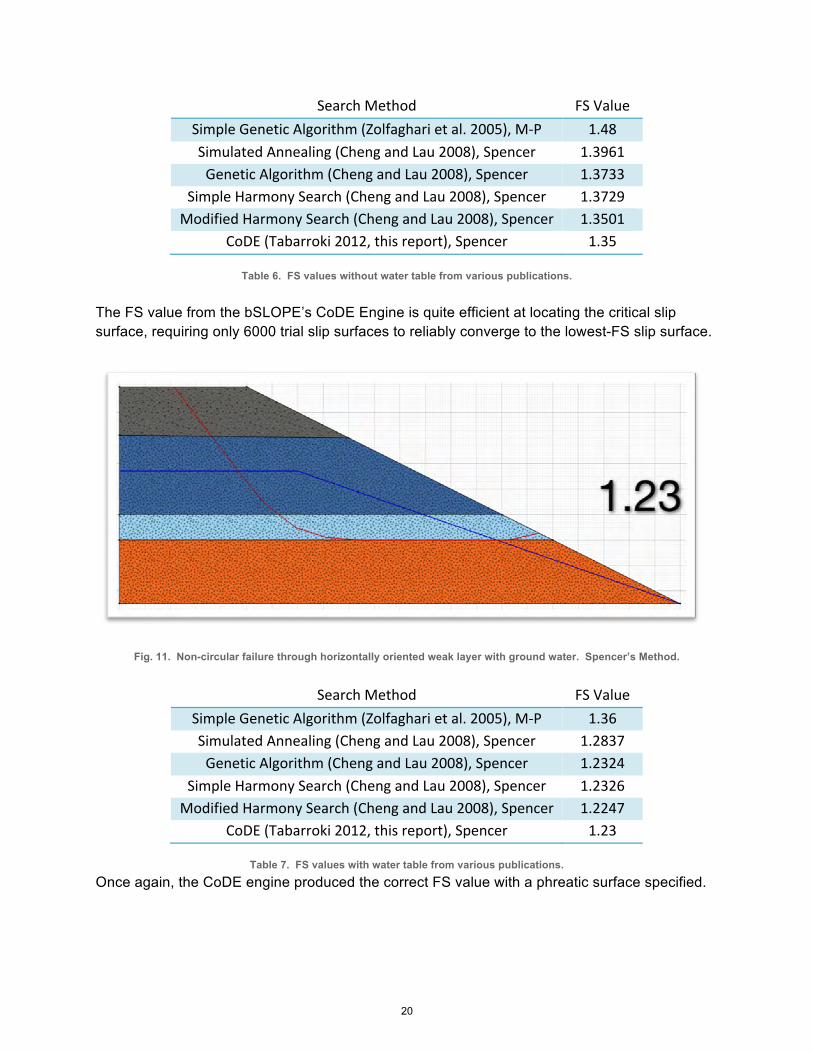
Table 6. FS values without water table from various publications. The FS value from the bSLOPE’s CoDE Engine is quite efficient at locating the critical slip surface, requiring only 6000 trial slip surfaces to reliably converge to the lowest-FS slip surface.

Fig. 11. Non-circular failure through horizontally oriented weak layer with ground water. Spencer’s Method.

Search Method FS Value Simple Genetic Algorithm (Zolfaghari et al. 2005), M-‐P 1.36 Simulated Annealing (Cheng and Lau 2008), Spencer 1.2837 Genetic Algorithm (Cheng and Lau 2008), Spencer 1.2324

Simple Harmony Search (Cheng and Lau 2008), Spencer 1.2326 Modified Harmony Search (Cheng and Lau 2008), Spencer 1.2247


Table 7. FS values with water table from various publications.

Once again, the CoDE engine produced the correct FS value with a phreatic surface specified.

20

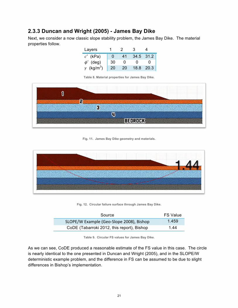
2.3.3 Duncan and Wright (2005) - James Bay Dike Next, we consider a now classic slope stability problem, the James Bay Dike. The material properties follow.

Layers 1 2 3 4 𝑐! (kPa) 0 41 34.5 31.2 𝜙′ (deg) 30 0 0 0 𝛾 (kg/m3) 20 20 18.8 20.3

Table 8. Material properties for James Bay Dike.

Fig. 11. James Bay Dike geometry and materials.

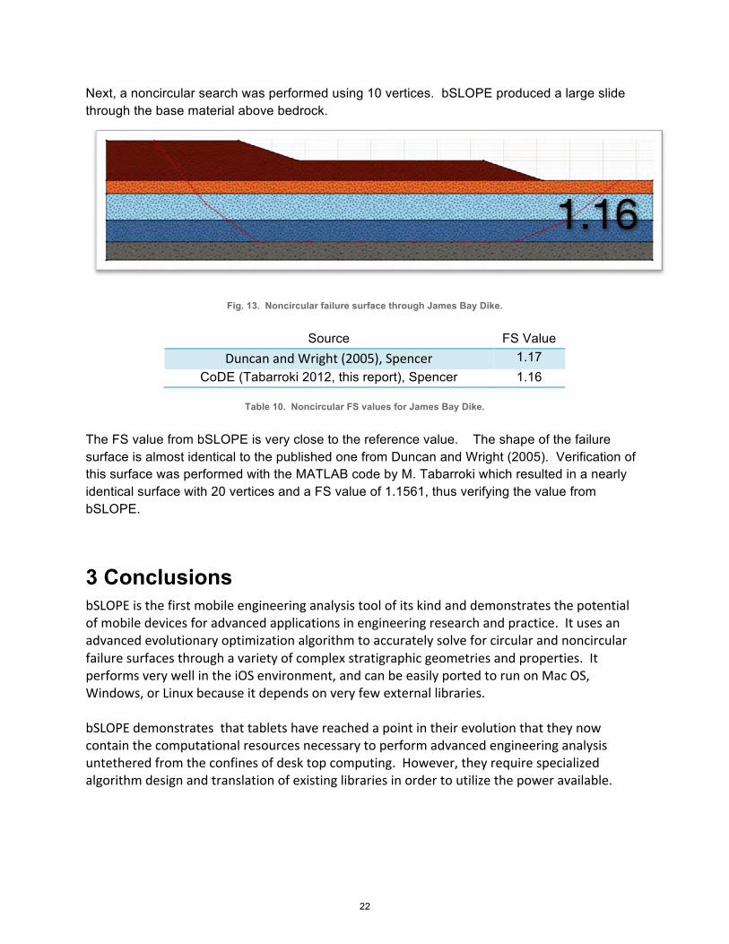
Fig. 12. Circular failure surface through James Bay Dike.

Source FS Value SLOPE/W Example (Geo-‐Slope 2008), Bishop 1.459 CoDE (Tabarroki 2012, this report), Bishop 1.44

Table 9. Circular FS values for James Bay Dike. As we can see, CoDE produced a reasonable estimate of the FS value in this case. The circle is nearly identical to the one presented in Duncan and Wright (2005), and in the SLOPE/W deterministic example problem, and the difference in FS can be assumed to be due to slight differences in Bishop’s implementation.

21

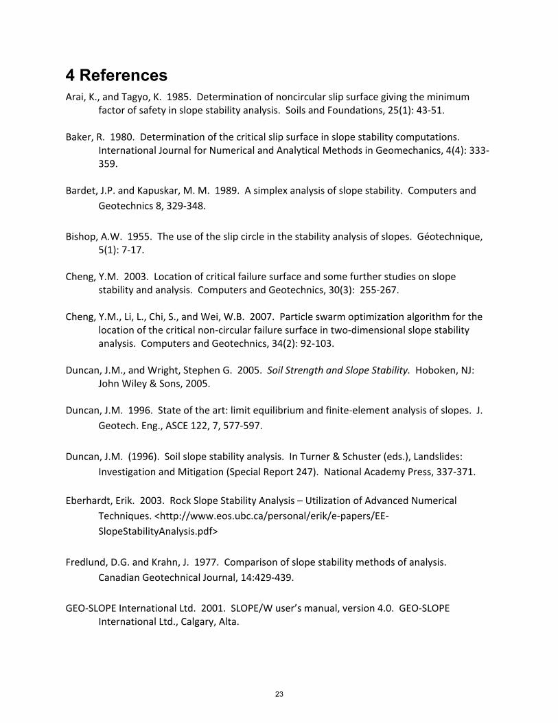
Next, a noncircular search was performed using 10 vertices. bSLOPE produced a large slide through the base material above bedrock.

Fig. 13. Noncircular failure surface through James Bay Dike.

Source FS Value

Duncan and Wright (2005), Spencer 1.17 CoDE (Tabarroki 2012, this report), Spencer 1.16

Table 10. Noncircular FS values for James Bay Dike. The FS value from bSLOPE is very close to the reference value. The shape of the failure surface is almost identical to the published one from Duncan and Wright (2005). Verification of this surface was performed with the MATLAB code by M. Tabarroki which resulted in a nearly identical surface with 20 vertices and a FS value of 1.1561, thus verifying the value from bSLOPE.

3 Conclusions bSLOPE is the first mobile engineering analysis tool of its kind and demonstrates the potential of mobile devices for advanced applications in engineering research and practice. It uses an advanced evolutionary optimization algorithm to accurately solve for circular and noncircular failure surfaces through a variety of complex stratigraphic geometries and properties. It performs very well in the iOS environment, and can be easily ported to run on Mac OS, Windows, or Linux because it depends on very few external libraries. bSLOPE demonstrates that tablets have reached a point in their evolution that they now contain the computational resources necessary to perform advanced engineering analysis untethered from the confines of desk top computing. However, they require specialized algorithm design and translation of existing libraries in order to utilize the power available.

22

4 References Arai, K., and Tagyo, K. 1985. Determination of noncircular slip surface giving the minimum

factor of safety in slope stability analysis. Soils and Foundations, 25(1): 43-‐51. Baker, R. 1980. Determination of the critical slip surface in slope stability computations.

International Journal for Numerical and Analytical Methods in Geomechanics, 4(4): 333-‐359.

Bardet, J.P. and Kapuskar, M. M. 1989. A simplex analysis of slope stability. Computers and

Geotechnics 8, 329-‐348. Bishop, A.W. 1955. The use of the slip circle in the stability analysis of slopes. Géotechnique,

5(1): 7-‐17. Cheng, Y.M. 2003. Location of critical failure surface and some further studies on slope

stability and analysis. Computers and Geotechnics, 30(3): 255-‐267. Cheng, Y.M., Li, L., Chi, S., and Wei, W.B. 2007. Particle swarm optimization algorithm for the

location of the critical non-‐circular failure surface in two-‐dimensional slope stability analysis. Computers and Geotechnics, 34(2): 92-‐103.

Duncan, J.M., and Wright, Stephen G. 2005. Soil Strength and Slope Stability. Hoboken, NJ:

John Wiley & Sons, 2005. Duncan, J.M. 1996. State of the art: limit equilibrium and finite-‐element analysis of slopes. J.

Geotech. Eng., ASCE 122, 7, 577-‐597. Duncan, J.M. (1996). Soil slope stability analysis. In Turner & Schuster (eds.), Landslides:

Investigation and Mitigation (Special Report 247). National Academy Press, 337-‐371. Eberhardt, Erik. 2003. Rock Slope Stability Analysis – Utilization of Advanced Numerical

Techniques. <http://www.eos.ubc.ca/personal/erik/e-‐papers/EE-‐SlopeStabilityAnalysis.pdf>

Fredlund, D.G. and Krahn, J. 1977. Comparison of slope stability methods of analysis.

Canadian Geotechnical Journal, 14:429-‐439. GEO-‐SLOPE International Ltd. 2001. SLOPE/W user’s manual, version 4.0. GEO-‐SLOPE

International Ltd., Calgary, Alta.

23

GEO-‐SLOPE International Ltd. 2008. Probability – James Bay Case History. SLOPE/W Example Problem. GEO-‐SLOPE International Ltd., Calgary, Alta.

Greco, V.R. 1996. Efficient Monte Carlo technique for locating critical slip surface. Journal of

Geotechnical Engineering, ASCE, 122, 517–525. Janbu, N. 1954. Application of composite slip surfaces for stability analysis. In Proceedings of

the European Conference on Stability of Earth Slopes. Stockholm, Sweden. Vol. 3, pp. 43-‐49.

Li, Yu-‐Chao, et al. 2010. An efficient approach for locating the critical slip surface in slope

stability analyses using a real-‐coded genetic algorithm. NRC Research Press Web Site. 25 June.

Morgenstern, N.R., and Price, V.E. 1965. The analysis of the stability of general slip surfaces.

Géotechnique, 15(1): 79-‐93. Nguyen, V.U. 1985. Determination of critical slope failure surfaces. J. Geotech. Eng. ASCE,

111:238-‐250. Pham, Ha T.V. and Fredlund, Delwyn G. 2003. The application of dynamic programming to

slope stability analysis. NRC Research Press, 11 August. <http://www.soilvision.com/downloads/docs/pdf/research/DynamicProgramming.pdf>

Sarma, S.K. 1973. Stability analysis of embankments and slopes. Géotechnique, 23(3): 423-‐

433. Sarma, S.K. 1979. Stability analysis of embankments and slopes. Journal of Geotechnical

Engineering, ASCE, 105(12): 1511-‐1524. Spencer, E. 1967. A method for analysis of the stability of embankments assuming parallel

interslice forces. Géotechnique, 17(1): 11-‐26. Tabarroki, M. 2012. Computer Aided Slope Stability Analysis Using Optimization and Parallel

Computing Techniques. M.Sc. thesis, University of Science Malaysia. Wang, Yong, et al. 2011. Differential Evolution with Composite Trial Vector Generation

Strategies and Control Parameters. Evolutionary Computation, IEEE Transactions on, vol.15, no.1, pp.55-‐66, Feb.

24

Zolfaghari, A.R., Heath, A.C., and McCombie, P.F. 2005 Simple genetic algorithm search for critical non-‐circular failure surface in slope stability analysis. Computers and Geotechnics, 32(3): 139-‐152.

25

Appendix A: Function Documentation

26

of 23

MWCoDEEngine.m 5/9/12 3:41 PM

//// MWCoDEEngine.m// bSLOPE//// Created by Oliver Rickard on 2/19/12.// Copyright (c) 2012 Mobile World Software. All rights reserved.// Port of MATLAB code by Mohammad Tabarroki, published// with his permission.//

#import "MWCoDEEngine.h"#import "SMUGMath.h"#include <Accelerate/Accelerate.h>#include "JSGCDDispatcher.h"#include "FSSlipPointsDataController.h"

/** This method uses the CoDE (Composite Differential Evolution, Yong Wang 2011

) to generate a new slip surface from an existing one. Input parameters are: RealMatrix *p: initial matrix in the form [x1,xn,sigma2,...sigman-1], where

sigmai is between 0 and 1. RealMatrix *lu: Lower and upper bounds for each x-coordinate, generated

through Cheng 2003 strategy. int i: current index of the slip surface. RealVector *F: Calibration parameter vector. Contains one F value for each

generation strategy. See Yong Wang 2011. RealVector *CR: Calibration parameter vector. Contains one CR value for

each generation strategy. See Yong Wang 2011. int popsize: size of the current population of slip surfaces. int n: selection index. RealVector *paraIndex: vector of parameter indices. These are randomized

from the set of F and CR for each slip surface. Output is a new RealMatrix of three row vectors which represent mutants of

the three vector generation strategies.*/static RealMatrix *generator(RealMatrix *p, RealMatrix *lu, int i,

RealVector *F, RealVector *CR, int popsize, int n, RealVector *paraIndex) { }

@implementation MWCoDEEngine

#pragma mark - Utility Functions for Circular Surfaces

/** This function is for circular slip surfaces. It simply computes the 2D

arctangent between 0 and 360 degrees. Input parameters are: float y: y-value float x: x-value Output is the float value of the 2-D arctangent of the x and y values.

27

of 23


*/+(float)atan2d_0_360Y:(float)y X:(float)x;{ }

/** This function is for circular slip surfaces. It finds the center of a

circle of Radius R which intersects points p1 and p2. Input parameters: CGPoint p1: CGPoint C struct value with x and y parameters. First point

value. CGPoint p2: CGPoint C struct value with x and y parameters. Second point

value. float R: float value representing the radius of the circle. Output is the CGPoint struct representing the center of the circle. */+(CGPoint)findCenterP1:(CGPoint)p1 P2:(CGPoint)p2 R:(float)R;{ }

/** This function is for circular slip surfaces. It finds the minimum radius

of a circle containing points p1 and p2. Input parameters: CGPoint p1: CGPoint C struct value with x and y parameters. First point

value. CGPoint p2: CGPoint C struct value with x and y parameters. Second point

value. Output is the float value of the radius.*/+(float)findMinR2P1:(CGPoint)p1 P2:(CGPoint)p2;{ }

#pragma mark - Utility Functions

/** This function finds the intersection between two lines defined by [p1,p2]

and [p3,p4]. Input Parameters: CGPoint p1: CGPoint C struct with x and y parameters. One of the points

defining a line. CGPoint p2: CGPoint C struct with x and y parameters. One of the points



defining a line. Output is a CGPoint value for the intersection between the two lines. */+(CGPoint)lineSegmentCrossP1:(CGPoint)p1 P2:(CGPoint)p2 P3:(CGPoint)p3 P4:

(CGPoint)p4;28

of 23


{ }

/** This interpolates between p1 and p2, with the restriction that the

interpolated value must be below the ground surface. If it is above the ground surface, then the value is interpolated in the ground matrix.

CGPoint p1: First point defining line, usually line between vertices on a slip surface. CGPoint C struct with x and y parameters.

CGPoint p2: Second point defining line, usually line between vertices on a slip surface. CGPoint C struct with x and y parameters.

RealMatrix *ground: Matrix of (x,y) row vectors of vertices of the ground surface.

Output is the interpolated y value. */+(float)lineOrBelowP1:(CGPoint)p1 P2:(CGPoint)p2 X:(float)x ground:

(RealMatrix *)ground;{ }

/** Function that generates a RealMatrix from an array of RealMatrix objects. Input Parameters: NSArray *arr: NSArray of RealMatrix objects. Do not have to be all the

same size. Output is a RealMatrix with each matrix appended to the bottom of a larger

matrix. The largest column number is taken for the output matrix, and zeros are inserted in the matrix for any matrices with less columns.

*/+(RealMatrix *)matrixFromArray:(NSArray *)arr;{ }

/** This function finds the radius of the moment arm betweent the point, and

the line defined by v1 and v2. Input parameters: CGPoint p1: Center of the rotation. CGPoint C struct with x and y

parameters. CGPoint v1: One of the points defining the direction of the force vector.

CGPoint C struct with x and y parameters. CGPoint v2: The other point defining the direction of the force vector.

CGPoint C struct with x and y parameters. Output is the float value of the radius of moment arm.*/+(float)getMomentArmPt:(CGPoint)pt V1:(CGPoint)v1 V2:(CGPoint)v2;{ }

/** This function computes the perpendicular offset of the normal placed at the

midpoint of [v1,v2] towards pt between the that normal ray, and pt. Input parameters:

29

of 23


CGPoint pt: CGPoint C struct with x and y parameters. This is the point that the distance is calculated from.

CGPoint v1: CGPoint C struct with x and y parameters. Defines one side of the line.

CGPoint v2: CGPoint C struct with x and y parameters. Defines other side of the line.

Output is the float distance from pt to the line normal to [v1,v2].*/+(float)point_prpnd_line:(CGPoint)pt V1:(CGPoint)v1 V2:(CGPoint)v2;{ }

/** This function computes a linearly interpolated yVal value between two

neighboring points. xVal must be between neighbor1.x and neighbor2.x, and neighbor1.x must be less than neighbor2.x.

Input Parameters: CGPoint neighbor1: This is the left neighbor of the point that needs to be

interpolated. CGPoint C struct with x and y parameters. CGPoint neighbor2: This is the right neighbor of the point that needs to be

interpolated. CGPoint C struct with x and y parameters. float xVal: This is the x value for which we want to interpolate a y value. Output is a float y interpolation. */+(float)interp:(CGPoint)neighbor1 neighbor2:(CGPoint)neighbor2 xVal:(float)

xVal;{ }

/** This function computes linearly interpolated yVal between two neighboring

points. neighbor1 and neighbor2 need not be in any particular order. The if tree is in place to ensure that the minimum possible number of comparisons is done for most use cases.

Input Parameters: CGPoint neighbor1: This is the first neighbor of the point that needs to be

interpolated. CGPoint C struct with x and y parameters. CGPoint neighbor2: This is the other neighbor of the point that needs to be

interpolated. CGPoint C struct with x and y parameters. float xVal: This is the x value for which we want to interpolate a y value. float defValue: Default interpolation value if xVal is not within the range

[neighbor1.x,neighbor2.x] or [neighbor2.x,neighbor1.x]. Output is the y value of the interpolation. If the xVal is not within the

correct range, then the default value will be returned. */+(float)safeInterp:(CGPoint)neighbor1 neighbor2:(CGPoint)neighbor2 xVal:

(float)xVal defValue:(float)defValue;{ }

/** This function performs a safeInterp on all of the values in xVals. Input Parameters:

30

of 23


CGPoint neighbor1: This is the first neighbor of the point that needs to be interpolated. CGPoint C struct with x and y parameters.

CGPoint neighbor2: This is the other neighbor of the point that needs to be interpolated. CGPoint C struct with x and y parameters.

RealVector *xVals: These are the x values for which we want to interpolate y values.

float defValue: Default interpolation value if xVal is not within the range [neighbor1.x,neighbor2.x] or [neighbor2.x,neighbor1.x].

Output is a vector of interpolated y values. If the xVal is not within the

correct range, then the default value will be inserted at that index. */+(RealVector *)safeInterp:(CGPoint)neighbor1 neighbor2:(CGPoint)neighbor2

xVals:(RealVector *)xVals defValue:(float)defValue;{ }

/** Linearly interpolates between the values in x and y for all x-values in xi.

Default value is inserted in the return vector for any values outside of x.

Input Parameters: RealVector *x: x-values for the points between which we want to interpolate

. RealVector *y: y-values for the points between which we want to interpolate

. RealVector *xi: x-values that we want to interpolate a y value. float defValue: Default value if a particular xi is not within the x range. Output is a vector of y-values at each xi. *///Linearly interpolates between the values (x,y) for all x-values in xi.+(RealVector *)lininterp1fX:(RealVector *)x Y:(RealVector *)y Xi:(RealVector

*)xi DefValue:(float)defValue;{ }

#pragma mark - GLE Implementation, non-circular

/** Newton Raphson method to provide a new lambda value. See Newton Raphson on

Wikipedia. Input Parameters: float FSm: FS from moment equilibrium. float FSmOld: Old FS from moment equilibrium. float FSf: FS from force equilibrium. float FSfOld: Old FS from force equilibrium float myLambda: Current lambda value. float myLambdaOld: old lambda value. Output is the new lambda given the input parameters. */+(float)newtonRaphsonFSm:(float)FSm FSmOld:(float)FSmOld FSf:(float)FSf

FSfOld:(float)FSfOld myLambda:(float)myLambda myLambdaOld:(float)myLambdaOld;

{ }31

of 23


/** This function computes the force-equilibrium FS value for the slices given

the parameters in the vector arguments. Computed according to the GLE formulation in Fredlund and Krahn.

Input parameters: RealVector *sCohesion: This is a vector containing one cohesion value for

the base of each slice. Units of kPa. RealVector *sLength: Vector containing the length of the line defining the

base of each slice. Units of m. RealVector *sAlpha: Vector containing the angle from horizontal of the line

defining the base of each slice. Units of degrees. RealVector *sN: Vector containing the normal force along the bottom of each

slice. Units of kPa. RealVector *sU: Vector containing the suction force along the bottom of

each slice. Units of kPa. RealVector *sFrictionAngle: Vector containing the internal friction angle

of the soil along the base of each slice. Units of degrees. Output is a float value for the force-equilibrium FS.*/+(float)GLEfsFSliceCohesion:(RealVector *)sCohesion sliceLength:(RealVector

*)sLength sliceAlpha:(RealVector *)sAlpha sliceN:(RealVector *)sN sliceU:(RealVector *)sU sliceFrictionAngle:(RealVector *)sFrictionAngle;

{ }

/** This function computes the moment-equilibrium FS value for the slices given

the parameters in the vector arguments. Computed according to the GLE formulation in Fredlund and Krahn.



base of each slice. Units of m. RealVector *sR: Vector containing the moment arm for each slice. Units of

m. RealVector *sAlpha: Vector containing the angle from horizontal of the line

defining the base of each slice. Units of degrees. RealVector *sN: Vector containing the normal force along the bottom of each



of the soil along the base of each slice. Units of degrees. RealVector *sWeight: Vector containing weight of the material in each slice

. Units of kN. RealVector *sf: Vector containing perpendicular offset of the normal force

from the center of rotation. Units of m. RealVector *sx: Vector containing horizontal distance from the slice to the

center of rotation. Units of m. Output is a float value for the moment-equilibrium FS. */

32

of 23


+(float)GLEfsMSliceCohesion:(RealVector *)sCohesion sliceLength:(RealVector *)sLength sliceR:(RealVector *)sR sliceN:(RealVector *)sN sliceU:(RealVector *)sU sliceFrictionAngle:(RealVector *)sFrictionAngle sliceWeight:(RealVector *)sWeight slicef:(RealVector *)sf slicex:(RealVector *)sx;

{ }

/** This function generates the sliceN vector, which is the total nomral force

on the base of each slice in vector form. Input parameters: RealVector *sWeight: Vector containing the weight of each slice. Units of

kN. RealVector *sXr_Xl: Vector containing the resultant of the vertical

interslice shear forces for each slice. Units of kPa. RealVector *sCohesion: This is a vector containing one cohesion value for


base of each slice. Units of m. RealVector *sAlpha: Vector containing the angle from horizontal of the line

defining the base of each slice. Units of degrees. RealVector *sU: Vector containing the suction force along the bottom of

each slice. Units of kPa. RealVector *sliceFrictionAngle: Vector containing the internal friction

angle of the soil along the base of each slice. Units of degrees. float trialF: The current FS for the current trial vector. Output is a vector of slice normal forces, sliceN.*///This function generates the sliceN vector, the total normal force on the

base of the slice.+(RealVector *)GLEsliceNSliceWeight:(RealVector *)sWeight sliceXr_Xl:

(RealVector *)sXr_Xl sliceCohesion:(RealVector *)sCohesion sliceLength:(RealVector *)sLength sliceAlpha:(RealVector *)sAlpha sliceU:(RealVector *)sU sliceFrictionAngle:(RealVector *)sFrictionAngle trialF:(float)trialF;

{ }

/** This function finds the FS using the ordinary method of slices (OMS), which

is the first stage of the GLE solution. Input Parameters: RealVector *sliceWeight: Vector containing weights of each slice. Units of

kN. RealVector *sliceAlpha: Vector containing the angle from horizontal of the

base of each slice. Units of degrees. RealVector *sliceCohesion: Vector containing cohesion value at the base of

each slice. Units of kPa. RealVector *sliceLength: Vector containing the length of the line that

defines the bottom of each slice. Units of m. RealVector *sliceFrictionAngle: Vector containing the friction angle of

each slice at the base. Units of degrees. RealVector *sliceU: Vector containing suction value at the base of each

slice. Units of kPa.33

of 23


RealVector *sliceR: Vector containing length of moment arm to where forces act. Units of m.

Output is the FS as a float value. */+(float)ordinaryFSBuilderv2SliceWeight:(RealVector *)sliceWeight sliceAlpha:

(RealVector *)sliceAlpha sliceCohesion:(RealVector *)sliceCohesion sliceLength:(RealVector *)sliceLength sliceFrictionAngle:(RealVector *)sliceFrictionAngle sliceU:(RealVector *)sliceU sliceR:(RealVector *)sliceR;

{ }

/** This function finds the GLE simplified Bishop FS for the given slip surface

. Input Parameters: float FSm: FS value for moment equilibrium as initial guess for this

function. float myPrecision: Decimal value defining the precision at which

convergence has been reached. Generally 0.001 to 0.00001. Floats are generally precise to 0.000001, though not always.

RealVector *sliceWeight: Vector containing weights of each slice. Units of kN.

RealVector *sliceCohesion: Vector containing cohesion value at the base of each slice. Units of kPa.

RealVector *sliceLength: Vector containing the length of the line that defines the bottom of each slice. Units of m.

RealVector *sliceAlpha: Vector containing the angle from horizontal of the base of each slice. Units of degrees.

RealVector *sliceU: Vector containing suction value at the base of each slice. Units of kPa.

RealVector *sliceFrictionAngle: Vector containing the friction angle of each slice at the base. Units of degrees.

RealVector *slicef: Vector containing perpendicular offset of the normal force from the center of rotation. Units of m.

RealVector *slicex: Vector containing horizontal distance from the slice to the center of rotation. Units of m.


unsigned int maxIteration: Maximum number of iterations before the slip surface is assumed to not converge.

Output is an array of moment-equilibrium FS and N value associated in an

NSArray, in that order. */+(NSArray *)gleBishopTrialF:(float)FSm myPrecision:(float)myPrecision

sliceWeight:(RealVector *)sliceWeight sliceCohesion:(RealVector *)sliceCohesion sliceLength:(RealVector *)sliceLength sliceAlpha:(RealVector *)sliceAlpha sliceU:(RealVector *)sliceU sliceFrictionAngle:(RealVector *)sliceFrictionAngle slicef:(RealVector *)slicef slicex:(RealVector *)slicex sliceR:(RealVector *)sliceR maxIteration:(unsigned int)maxIteration;

{ }

/**34

of 23


This function finds the GLE simplified Janbu FS for the given slip surface. Input Parameters: float FSf: FS value for force equilibrium as initial guess for this










Output is an array of force-equilibrium FS and N value associated in an

NSArray, in that order. */+(NSArray *)gleJanbuTrialF:(float)FSf myPrecision:(float)myPrecision

sliceWeight:(RealVector *)sliceWeight sliceCohesion:(RealVector *)sliceCohesion sliceLength:(RealVector *)sliceLength sliceAlpha:(RealVector *)sliceAlpha sliceU:(RealVector *)sliceU sliceFrictionAngle:(RealVector *)sliceFrictionAngle maxIteration:(unsigned int)maxIteration;

{ }

/** This function finds the inter-slice horizontal force resultant from the

difference between right and left side. Done for each slice, and stored in a vector.

Input Parameters: RealVector *sliceCohesion: Vector containing cohesion value at the base of


defines the bottom of each slice. Units of m. RealVector *sliceN: Vector containing the normal force along the bottom of

each slice. Units of kPa. RealVector *sliceAlpha: Vector containing the angle from horizontal of the

base of each slice. Units of degrees. RealVector *sliceU: Vector containing suction value at the base of each

slice. Units of kPa. RealVector *sliceFrictionAngle: Vector containing the friction angle of

each slice at the base. Units of degrees. float trialF: Current trial FS float value. Output is a vector of the Er-El float value at each slice. */

35

of 23


+(RealVector *)GLESliceEr_ElSliceCohesion:(RealVector *)sliceCohesion sliceLength:(RealVector *)sliceLength sliceN:(RealVector *)sliceN sliceAlpha:(RealVector *)sliceAlpha sliceU:(RealVector *)sliceU sliceFrictionAngle:(RealVector *)sliceFrictionAngle trialF:(float)trialF;

{ }

/** This function computes the force-equilibrium for a slip surface. This is

the last stage of the force GLE solution. Input Parameters: float FSf: Initial guess for force-equilibrium for the current slip surface

. float myPrecision: Decimal representing the precision at which convergence

is assumed to have occurred. Generally 0.001 to 0.00001. RealVector *sliceWeight: Vector containing weights of each slice. Units of

kN. RealVector *sliceCohesion: Vector containing cohesion value at the base of


defines the bottom of each slice. Units of m. RealVector *sliceAlpha: Vector containing the angle from horizontal of the

base of each slice. Units of degrees. RealVector *sliceU: Vector containing suction value at the base of each

slice. Units of kPa. RealVector *sliceFrictionAngle: Vector containing the friction angle of

each slice at the base. Units of degrees. RealVector *sliceNf: Vector containing initial N value guess. float myLambda: Current lambda value from either an initial guess or the

Newton-Raphson method. unsigned int maxIteration: Maximum number of iterations before the slip

surface is assumed to not converge. Output is a NSArray of the force-equilibrium FS and the associated N value,

in that order. */+(NSArray *)gleSolverFSf:(float)FSf myPrecision:(float)myPrecision

sliceWeight:(RealVector *)sliceWeight sliceCohesion:(RealVector *)sliceCohesion sliceLength:(RealVector *)sliceLength sliceAlpha:(RealVector *)sliceAlpha sliceU:(RealVector *)sliceU sliceFrictionAngle:(RealVector *)sliceFrictionAngle sliceNf:(RealVector *)sliceNf myLambda:(float)myLambda maxIteration:(unsigned int)maxIteration;

{ }

/** This function computes the moment-equilibrium for a slip surface. This is

the last stage of the moment GLE solution. Input Parameters: float FSm: Initial guess for moment-equilibrium for the current slip

surface. float myPrecision: Decimal representing the precision at which convergence

is assumed to have occurred. Generally 0.001 to 0.00001. RealVector *sliceWeight: Vector containing weights of each slice. Units of

kN.36

of 23







RealVector *slicef: Vector containing perpendicular offset of the normal force from the center of rotation. Units of m.

RealVector *slicex: Vector containing horizontal distance from the slice to the center of rotation. Units of m.


RealVector *sliceNm: Vector containing initial guess of N value. float myLambda: Current lambda value from either an initial guess or the

Newton-Raphson method. unsigned int maxIteration: Maximum number of iterations before the slip

surface is assumed to not converge. Output is a NSArray of the moment-equilibrium FS and the associated N value

, in that order. */+(NSArray *)gleSolverFSm:(float)FSm myPrecision:(float)myPrecision

sliceWeight:(RealVector *)sliceWeight sliceCohesion:(RealVector *)sliceCohesion sliceLength:(RealVector *)sliceLength sliceAlpha:(RealVector *)sliceAlpha sliceU:(RealVector *)sliceU sliceFrictionAngle:(RealVector *)sliceFrictionAngle slicef:(RealVector *)slicef slicex:(RealVector *)slicex sliceR:(RealVector *)sliceR sliceNm:(RealVector *)sliceNm myLambda:(float)myLambda maxIteration:(unsigned int)maxIteration;

{ }

/** This function is the primary analyzer engine that finds the FS for the

failure surface specified in slipPoints. It uses the GLE to determine Morgenstern-Price and Spencer FS.

Input Parameters: float gammaWater: Specific weight of water. Units of kN/m3. RealMatrix *slipPoints: Matrix of (x,y) row vectors defining the current

slip surface. CGPoint axisPoint: CGPoint C struct with x and y parameters. Point about

which moments are computed. RealMatrix *nonEdgeLines: Matrix of (x,y) row-vectors that define the outer

boundaries of the slope. RealMatrix *edgeLines: Matrix of (x,y) row-vectors that define the

boundaries between stratigraphic units inside of the slope. RealMatrix *materials: Matrix of material properties. Each material is a

column vector. RealMatrix *phreaticLine: Matrix of (x,y) row-vectors that define the path

of the phreatic surface within the slope. float myPrecision: Decimal representing precision at which convergence is

assumed to have occurred.37

of 23



Output is the converged FS value for the given failure surface. */+(float)analyzerEngineNonCircGammaWater:(float)gammaWater slipPoints:

(RealMatrix *)slipPoints axisPoint:(CGPoint)axisPoint nonEdgeLines:(RealMatrix *)nonEdgeLines edgeLines:(RealMatrix *)edgeLines materials:(RealMatrix *)materials phreaticLine:(RealMatrix *)phreaticLine myPrecision:(float)myPrecision maxIteration:(unsigned int)maxIteration;

{ }

/** This function is the real workhorse of the app. It takes an initial

population of "pos" vectors that define slip surfaces, then it generates failure surfaces for those vectors, and evaluates the FS for them using the GLE from Fredlund and Krahn. This is the single-threaded function.

Input Parameters: RealMatrix *pos: Matrix of "pos" row vectors. The first two values in the

row are the entry and exit x values, then the rest of the values are the vertical placement of the vertex between 0 and 1.

CGPoint axisPoint: CGPoint C struct with x and y parameters. This is the center about which moments are computed.

unsigned int noSlice: This is the number of slices for each slip surface. float tolSlicing: Minimum width of a slice before it is removed. RealMatrix *nonEdgeLines: Matrix of (x,y) row-vectors that define the outer





assumed to have occurred. unsigned int maxIteration: Maximum number of iterations before the slip

surface is assumed to not converge. RealMatrix *ground: Matrix of (x,y) row vectors representing the top of the

cross section. Realmatrix *bedrock: Matrix of (x,y) row vectors representing the bottom of

the cross section. float gammaWater: Specific weight of water. Units of kN/m3. NSMutableArray *layersCord: Array of polygons defining stratigraphic layers

. Each polygon is a RealMatrix with (x,y) row vector. completionBlock: This is an Objective-C block to execute upon completion of

FS evaluations. This is here to retain the same method signature between the single-threaded and multithreaded versions of this function.

Output is stored in the FSSlipPointsController singleton as an array of FS

values, and an array of RealMatrix slip points. */+(void)FSsEvalPos:(RealMatrix *)pos axisPoint:(CGPoint)axisPoint noSlice:

(unsigned int)noSlice tolSlicing:(float)tolSlicing nonEdgeLines:38

of 23


(RealMatrix *)nonEdgeLines edgeLines:(RealMatrix *)edgeLines materials:(RealMatrix *)materials phreaticLine:(RealMatrix *)phreaticLine myPrecision:(float)myPrecision maxIteration:(unsigned int)maxIteration ground:(RealMatrix *)ground bedrock:(RealMatrix *)bedrock gammaWater:(float)gammaWater layersCord:(NSMutableArray *)layersCord completionBlock:(void (^)())completionBlock;

{ }

#pragma mark - Slice Info Methods

/** This function gets the weight of a given slice. Input Parameters: float sWidth: Width of the given slice. Units of m. RealVector *yVals: Vector containing the y-values of the slice's centerline

with the stratigraphic boundaries. Units of m. RealVector *matVals: Vector containing the material indices for each

stratigraphic layer that the slice intersects. RealVector *materialsWeight: Vector containing the material weights for all

materials. Output is the weight of the slice in units of kN.*/+(float)slWeightBuilderSliceWidth:(float)sWidth yVals:(RealVector *)yVals

matVals:(RealVector *)matVals materialsWeight:(RealVector *)materialsWeight;

{ }

/** This function builds the sliceInfo matrix which contains the relevant

parameters for each slice. Input Parameters: float gammaWater: Specific weight of water. Units of kN/m3. RealMatrix *slipPoints: Matrix representation of the slipPoints that define

the failure surface. Matrix of (x,y) row-vectors. RealMatrix *nonEdgeLines: Matrix of (x,y) row-vectors that define the outer




of the phreatic surface within the slope. CGPoint axisPoint: CGPoint C struct with x and y parameters. This is the

center of rotation for the FS calculations. Output is the sliceInfo matrix that contains rows in this order:

sliceWeight, sliceAlpha, sliceCohesion, sliceWidth, sliceFrictionAngle, sliceU, slicef, sliceR, slicex.

*/+(RealMatrix *)sliceInfoBuilderv2GammaWater:(float)gammaWater slipPoints:

(RealMatrix *)slipPoints nonEdgeLines:(RealMatrix *)nonEdgeLines edgeLines:(RealMatrix *)edgeLines materials:(RealMatrix *)materials phreaticLine:(RealMatrix *)phreaticLine axisPoint:(CGPoint)axisPoint;

39

of 23


{ }

/** This function generates additional vertices for the failure

surfacecontained in origSlipPoints according to the rules in Cheng. Input Parameters: NSMutableArray *layersCord: Array of RealMatrix objects which define the

stratigraphic elements in the cross section as polygons. Each RealMatrix has (x,y) row vectors.

RealMatrix *origSlipPoints: Original matrix of slip points that compose the failure surface. (x,y) row vectors.

Output is a RealMatrix of the origSlipPoints, plus the new inserted points.*/+(RealMatrix *)moreSlicesRegionPointsLayersCord:(NSMutableArray *)layersCord

slipPoints:(RealMatrix *)origSlipPoints;{ }

/** This function generates additional vertices for the failure

surfacecontained in origSlipPoints according to the rules in Cheng. Input Parameters: NSMutableArray *layersCord: Array of RealMatrix objects which define the


RealMatrix *slip: Original matrix of slip points that compose the failure surface. (x,y) row vectors.

Output is a RealMatrix of the slip, plus the new inserted points. */+(RealMatrix *)moreSlicesCrossBoundaryLayersCord:(NSMutableArray *)

layersCord slipPoints:(RealMatrix *)slip;{ }

/** This method refines the mesh of slices. It starts by adding slices at

important locations such as where the slip surface crosses stratigraphic boundaries. Picks the biggest slice and splits it until it reaches the specified number of slices (noSlice).

Input Parameters: NSMutableArray *layersCord: Array of RealMatrix objects which define the



unsigned int noSlice: Number of slices for each slip surface. float tolSlicing: The smallest allowed slice width. Any smaller, and the

slice is removed from the slip surface. Output is the matrix defining the new slip surface with the added points.*/+(RealMatrix *)moreSlicesLayersCord:(NSMutableArray *)layersCord slipPoints:

(RealMatrix *)origSlipPoints noSlice:(unsigned int)noSlice tolSlicing:40

of 23


(float)tolSlicing;{ }

#pragma mark - Problem Setup Functions

/** This function extracts the top and bottom boundaries of the cross section

from the nonEdgeLines matrix. Input Parameters: RealMatrix *nonEdgeLines: Matrix of (x,y) row vectors defining the lines

that make up the exterior boundary of the cross-section. Output is an NSArray of the top (ground) and bottom (bedrock) of the cross

section.*/+(NSArray *)grndBdrckExtractorNonEdgeLines:(RealMatrix *)nonEdgeLines;{ }

/** This function examines the array of stratigraphic layers, and builds a

matrix of internal (edgeLines) and exterior (nonEdgeLines) edges. Input Parameters: NSMutableArray *layersCord: Array of RealMatrix objects which define the


Output is the array of edgeLines and nonEdgeLines matrices with (x,y) row

vectors.*/+(NSArray *)edgeAndNonEdgeLayersCord:(NSMutableArray *)layersCord;{ }

#pragma mark - CoDE Methods

/** This function generates the lower and upper range of potential x values for

the entry and exit points, and the vertical positioning of each vertex in the failure surface (sigma in the paper).

Input Parameters: RealVector *xStartRange: Vector containing two values that define the range

of acceptable entry points for a slip surface through the cross section.

RealVector *xEndRange: Vector containing two values that define the range of acceptable exit points for a slip surface through the cross section.

unsigned int noVertices: The number of vertices in the slip surface. Output is a RealVector of length noVertices and with two rows. The first

row is the lower bound of potential slip surfaces, and the second row is the upper bound. This matrix is called "lu" for lower-upper in other parts of the code.

*/+(RealMatrix *)luGeneratorV2XStartRange:(RealVector *)xStartRange xEndRange:

(RealVector *)xEndRange noVertices:(unsigned int)noVertices;41

of 23


{ }

/** This function generates the x and y values for a slip surface based on the

upper boundary (ground), bottom boundary (bedrock), and the vector with the beginning and end x values, then the sigma values in a vector called pos.

Input Parameters: RealMatrix *ground: Matrix of (x,y) row vectors defining the top boundary

of the cross section. RealMatrix *bedrock: Matrix of (x,y) row vectors defining the bottom

boundary of the cross section. RealVector *pos: Vector with the entry and exit x-values, and sigma values

between 0 and 1 that define each slip vertex's y-location between the lower and upper boundary for each x value between the beginning and end.

Output is the RealMatrix of (x,y) row vectors of the generated slip surface

, after processing the pos vector.*/+(RealMatrix *)slipGeneratorNonConvexV2Ground:(RealMatrix *)ground bedrock:

(RealMatrix *)bedrock pos:(RealVector *)pos;{ }

/** This function is the Composite Differential Evolution algorithm. See Yong

Wang 2011 and attached paper for info on its implementation. Input Parameters: unsigned int popsize: Population size of the slip surfaces to be evolved. unsigned int noSlice: Number of slices in each slip surface. unsigned int Niter: The number of successive iterations of evolution of the

population of slip surfaces. CGPoint axisPoint: CGPoint C struct with x and y parameters. Point about

which rotation is calculated. unsigned int noVertice: Number of initial vertices to generate for the slip

surfaces. float myPrecision: Decimal used to judge whether or not convergence has

been reached. Generally 0.001 to 0.00001. unsigned int maxIteration: Maximum number of iterations for each slip

surface FS evaluation. RealMatrix *ground: Matrix of (x,y) row vectors representing the top of the


the cross section. RealVector *xStartRange: Vector containing two values that define the range



float tolSlicing: Minimum width of a slice before it is removed. RealMatrix *nonEdgeLines: Matrix of (x,y) row-vectors that define the outer


boundaries between stratigraphic units inside of the slope.42

of 23


RealMatrix *materials: Matrix of material properties. Each material is a column vector.

RealMatrix *phreaticLine: Matrix of (x,y) row-vectors that define the path of the phreatic surface within the slope.

float gammaWater: Specific weight of water. Units of kN/m3. NSMutableArray *layersCord: Array of polygons defining stratigraphic layers

. Each polygon is a RealMatrix with (x,y) row vector. NSObject *notified: Object to be notified on the progress of the CoDE

Engine. Output is an array of the slip surface, and the FS value for the lowest-FS

slip surface, in that order.*/+(NSArray *)CoDEEnginePopsize:(unsigned int)popsize noSlice:(unsigned int)

noSlice Niter:(unsigned int)Niter axisPoint:(CGPoint)axisPoint noVertice:(unsigned int)noVertice myPrecision:(float)myPrecision maxIteration:(unsigned int)maxIteration ground:(RealMatrix *)ground bedrock:(RealMatrix *)bedrock xStartRange:(RealVector *)xStartRange xEndRange:(RealVector *)xEndRange tolSlicing:(float)tolSlicing nonEdgeLines:(RealMatrix *)nonEdgeLines edgeLines:(RealMatrix *)edgeLines materials:(RealMatrix *)materials phreaticLine:(RealMatrix *)phreaticLine gammaWater:(float)gammaWater layersCord:(NSMutableArray *)layersCord notified:(NSObject *)notified;

{ }

#pragma mark - Main CoDE Function

/** This function is what gets called by the user interface to begin a

computation. All that is needed to begin a computation are these four objects.

Input Parameters: NSMutableArray *layersCord: Array of polygons defining stratigraphic layers

. Each polygon is a RealMatrix with (x,y) row vector. RealVector *xStartRange: Vector containing two values that define the range



NSObject *notified: Object to be notified on the progress of the CoDE Engine. Generally the object that calls this function. The updateCoDEProgress:(float)progress function is called with a value from 0 to 1 signifying the completion of the task.

This function terminates without a direct output. It calls the

setSlipSurface:(RealMatrix *)slipSurface and setFS:(float)FS functions on the notified object.

*/+ (void)mainCoDE:(NSMutableArray *)layersCord materials:(RealMatrix *)

materials phreaticLine:(RealMatrix *)phreaticLine xStartRange:(RealVector *)xStartRange xEndRange:(RealVector *)xEndRange nonCircular:(BOOL)nonCircular notified:(NSObject *)notified;

{ }

43

of 23


#pragma mark - Circular CoDE Implementation/** This function is the Composite Differential Evolution algorithm. See Yong

Wang 2011 and attached paper for info on its implementation. Input Parameters: unsigned int popsize: Population size of the slip surfaces to be evolved. unsigned int noSlice: Number of slices in each slip surface. unsigned int Niter: The number of successive iterations of evolution of the

population of slip surfaces. CGPoint axisPoint: CGPoint C struct with x and y parameters. Point about

which rotation is calculated. unsigned int noVertice: Number of initial vertices to generate for the slip

surfaces. float myPrecision: Decimal used to judge whether or not convergence has

been reached. Generally 0.001 to 0.00001. unsigned int maxIteration: Maximum number of iterations for each slip

surface FS evaluation. RealMatrix *ground: Matrix of (x,y) row vectors representing the top of the


the cross section. RealVector *xStartRange: Vector containing two values that define the range



float tolSlicing: Minimum width of a slice before it is removed. RealMatrix *nonEdgeLines: Matrix of (x,y) row-vectors that define the outer




of the phreatic surface within the slope. float gammaWater: Specific weight of water. Units of kN/m3. NSMutableArray *layersCord: Array of polygons defining stratigraphic layers

. Each polygon is a RealMatrix with (x,y) row vector. NSObject *notified: Object to be notified on the progress of the CoDE

Engine. Output is an array of the slip surface, and the FS value for the lowest-FS

slip surface, in that order. */+(NSArray *)CoDEEngineCircPopsize:(unsigned int)popsize noSlice:(unsigned

int)noSlice maxRFactor:(int)maxRFactor Niter:(unsigned int)Niter axisPoint:(CGPoint)axisPoint myPrecision:(float)myPrecision maxIteration:(unsigned int)maxIteration ground:(RealMatrix *)ground bedrock:(RealMatrix *)bedrock xStartRange:(RealVector *)xStartRange xEndRange:(RealVector *)xEndRange tolSlicing:(float)tolSlicing nonEdgeLines:(RealMatrix *)nonEdgeLines edgeLines:(RealMatrix *)edgeLines materials:(RealMatrix *)materials phreaticLine:(RealMatrix *)

44

of 23


phreaticLine gammaWater:(float)gammaWater layersCord:(NSMutableArray *)layersCord notified:(NSObject *)notified;

{ }

/** This function generates the lower and upper range of potential x values for

the entry and exit points, radius for the slip surface. Input Parameters: RealVector *xStartRange: Vector containing two values that define the range



Output is a RealVector of length 3 and with two rows. The first row is the

lower bound of potential slip surfaces, and the second row is the upper bound. This matrix is called "lu" for lower-upper in other parts of the code.

*/+(RealMatrix *)luGeneratorCircXStartRange:(RealVector *)xStartRange

xEndRange:(RealVector *)xEndRange;{ }

/** This function generates the x and y values for a slip surface based on the

upper boundary (ground), bottom boundary (bedrock), and the vector with the beginning and end x values, radius sigma in V.

Input Parameters: int numSlice: number of slices to construct from the circular failure

surface. RealMatrix *ground: Matrix of (x,y) row vectors defining the top boundary

of the cross section. RealMatrix *bedrock: Matrix of (x,y) row vectors defining the bottom

boundary of the cross section. RealVector *V: Vector with the entry and exit x-values, and one sigma

values between 0 and 1 that defines the radius. Output is the RealMatrix of (x,y) row vectors of the generated slip surface

, after processing the pos vector. */+(NSArray *)slipGeneratorCircNumSlice:(int)numSlice ground:(RealMatrix *)

ground bedrock:(RealMatrix *)bedrock maxRFactor:(float)maxRFactor V:(RealVector *)V;

{ }

#pragma mark - Circular GLE Implementation

/** This function computes the circular moment-equilibrium FS value for the

slices given the parameters in the vector arguments. Computed according to the GLE formulation in Fredlund and Krahn.


45

of 23



base of each slice. Units of m. RealVector *sN: Vector containing the normal force along the bottom of each



of the soil along the base of each slice. Units of degrees. RealVector *sWeight: Vector containing weight of the material in each slice

. Units of kN. RealVector *sAlpha: Vector containing the angle from horizontal of the line

defining the base of each slice. Units of degrees. Output is a float value for the circular moment-equilibrium FS. */+(float)GLEfsMCircSliceCohesion:(RealVector *)sCohesion sliceLength:

(RealVector *)sLength sliceN:(RealVector *)sN sliceU:(RealVector *)sU sliceFrictionAngle:(RealVector *)sFrictionAngle sliceWeight:(RealVector *)sWeight sliceAlpha:(RealVector *)sAlpha;

{ }

/** This function finds the circular FS using the ordinary method of slices

(OMS), which is the first stage of the GLE solution. Input Parameters: RealVector *sliceWeight: Vector containing weights of each slice. Units of

kN. RealVector *sliceAlpha: Vector containing the angle from horizontal of the

base of each slice. Units of degrees. RealVector *sliceCohesion: Vector containing cohesion value at the base of


defines the bottom of each slice. Units of m. RealVector *sliceFrictionAngle: Vector containing the friction angle of

each slice at the base. Units of degrees. RealVector *sliceU: Vector containing suction value at the base of each

slice. Units of kPa. Output is the FS as a float value. */+(float)ordinaryFSBuilderv2CircSliceWeight:(RealVector *)sliceWeight

sliceAlpha:(RealVector *)sliceAlpha sliceCohesion:(RealVector *)sliceCohesion sliceLength:(RealVector *)sliceLength sliceFrictionAngle:(RealVector *)sliceFrictionAngle sliceU:(RealVector *)sliceU;

{ }

/** This function finds the circular simplified Bishop FS for the given slip

surface. Input Parameters: float FSm: FS value for moment equilibrium as initial guess for this


46

of 23










Output is an array of moment-equilibrium FS and N value associated in an

NSArray, in that order. */+(NSArray *)gleBishopCircTrialF:(float)FSm myPrecision:(float)myPrecision

sliceWeight:(RealVector *)sliceWeight sliceCohesion:(RealVector *)sliceCohesion sliceLength:(RealVector *)sliceLength sliceAlpha:(RealVector *)sliceAlpha sliceU:(RealVector *)sliceU sliceFrictionAngle:(RealVector *)sliceFrictionAngle maxIteration:(unsigned int)maxIteration;

{ }

/** This function is the primary analyzer engine that finds the circular FS for

the failure surface specified in slipPoints. It uses the GLE to determine Spencer FS.

Input Parameters: RealMatrix *slipPoints: Matrix of (x,y) row vectors defining the current

slip surface. float gammaWater: Specific weight of water. Units of kN/m3. RealMatrix *nonEdgeLines: Matrix of (x,y) row-vectors that define the outer






surface is assumed to not converge. Output is the converged FS value for the given failure surface. If

convergence is not achieved, or the slip is not admissable, then 99999 is returned for FS. The CoDE engine then evolves the slip surface to avoid inadmissable or non-computable surfaces.

*/+(float)analyzerEngineCircSlipPoints:(RealMatrix *)slipPoints gammaWater:

47

of 23


(float)gammaWater nonEdgeLines:(RealMatrix *)nonEdgeLines edgeLines:(RealMatrix *)edgeLines materials:(RealMatrix *)materials phreaticLine:(RealMatrix *)phreaticLine myPrecision:(float)myPrecision maxIteration:(unsigned int)maxIteration;

{ }

/** This function is the circular workhorse of the app. It takes an initial

population of "pos" vectors that define slip circles, then it generates failure surfaces for those vectors, and evaluates the FS for them using the GLE from Fredlund and Krahn. This is the single-threaded function.

Input Parameters: RealMatrix *pos: Matrix of "pos" row vectors. The first two values in the

row are the entry and exit x values, then the rest of the values are the vertical placement of the vertex between 0 and 1.

unsigned int noSlice: This is the number of slices for each slip surface. int maxRFactor: This is the maximum radius multiplier that is allowed for

the circle. float tolSlicing: Minimum width of a slice before it is removed. RealMatrix *nonEdgeLines: Matrix of (x,y) row-vectors that define the outer






surface is assumed to not converge. RealMatrix *ground: Matrix of (x,y) row vectors representing the top of the


the cross section. float gammaWater: Specific weight of water. Units of kN/m3. NSMutableArray *layersCord: Array of polygons defining stratigraphic layers

. Each polygon is a RealMatrix with (x,y) row vector. completionBlock: This is an Objective-C block to execute upon completion of

FS evaluations. This is here to retain the same method signature between the single-threaded and multithreaded versions of this function.

Output is stored in the FSSlipPointsController singleton as an array of FS

values, and an array of RealMatrix slip points. */+(void)FSsEvalCircPos:(RealMatrix *)pos axisPoint:(CGPoint)axisPoint

noSlice:(unsigned int)noSlice maxRFactor:(int)maxRFactor tolSlicing:(float)tolSlicing nonEdgeLines:(RealMatrix *)nonEdgeLines edgeLines:(RealMatrix *)edgeLines materials:(RealMatrix *)materials phreaticLine:(RealMatrix *)phreaticLine myPrecision:(float)myPrecision maxIteration:(unsigned int)maxIteration ground:(RealMatrix *)ground bedrock:(RealMatrix *)bedrock gammaWater:(float)gammaWater layersCord:(NSMutableArray *)layersCord completionBlock:(void (^)())completionBlock;

48

of 23


{ }

#pragma mark - Circular Slice Info Functions

/** This function builds the sliceInfo matrix which contains the relevant

parameters for each slice. Input Parameters: float gammaWater: Specific weight of water. Units of kN/m3. RealMatrix *slipPoints: Matrix representation of the slipPoints that define

the failure surface. Matrix of (x,y) row-vectors. RealMatrix *nonEdgeLines: Matrix of (x,y) row-vectors that define the outer




of the phreatic surface within the slope. Output is the sliceInfo matrix that contains rows in this order:

sliceWeight, sliceAlpha, sliceCohesion, sliceWidth, sliceFrictionAngle, sliceU.

*/+(RealMatrix *)sliceInfoBuilderv2CircGammaWater:(float)gammaWater

slipPoints:(RealMatrix *)slipPoints nonEdgeLines:(RealMatrix *)nonEdgeLines edgeLines:(RealMatrix *)edgeLines materials:(RealMatrix *)materials phreaticLine:(RealMatrix *)phreaticLine;

{ }

/** This method refines the mesh of slices. It starts by adding slices at

important locations such as where the slip surface crosses stratigraphic boundaries. Then it ensures that the slip surfaces have vertices wherever strata above them contain discontinuities. Finally, picks the biggest slice and splits it until it reaches the specified number of slices (noSlice).

Input Parameters: NSMutableArray *layersCord: Array of RealMatrix objects which define the



float tolSlicing: The smallest allowed slice width. Any smaller, and the slice is removed from the slip surface.

Output is the matrix defining the new slip surface with the added points. */+(RealMatrix *)moreSlicesCircLayersCord:(NSMutableArray *)layersCord

slipPoints:(RealMatrix *)origSlipPoints tolSlicing:(float)tolSlicing;{ }

@end

49

bSLOPE: A General Limit Equilibrium Slope Stability Analysis Code ...

Documents

Transcript of bSLOPE: A General Limit Equilibrium Slope Stability Analysis Code ...