Bsc Project MASTER

2015

408MHz Radio Telescope Supervisor: Leon Ellison

PH3110 Thomas Leigh Student No.100712227

Abstract:

A Radio Telescope can be used to identify celestial bodies unavailable to optical telescopes. A survey

of the sky will be completely different to that seen with the eye. This project focuses on the

procedures, design and problems of building a working Radio telescope. 408MHz is used specifically

because it is a reserved radio astronomy frequency. The type of telescope is a phase switched

interferometer with paired yagis antenna arrays. The techniques covered in this project will focus on

the concepts of signal gain, noise and radio astronomy.

Experimental or Theoretical Project – Thomas Leigh 1000712227

1

Table of Contents Abstract: ........................................................................................................................................................ 0

Introduction .................................................................................................................................................. 2

Radio astronomy ....................................................................................................................................... 2

Noise ......................................................................................................................................................... 4

The types of noise: ................................................................................................................................ 4

External noise ........................................................................................................................................ 7

Man-made or Interference noise .......................................................................................................... 7

Signal-to-noise ratio (SNR) .................................................................................................................... 8

Power supplies and Voltage drift .............................................................................................................. 8

Interferometry and its relevance to Radio astronomy ............................................................................. 9

Phase switch ........................................................................................................................................... 11

Standing wave ratio .................................................................................................................................. 9

The plan for the radio telescope ................................................................................................................. 13

Testing components ....................................................................................... Error! Bookmark not defined.

The oscilloscope: ..................................................................................................................................... 26

Signal generator ...................................................................................................................................... 26

Type of connectors ................................................................................................................................. 27

Testing the previous year’s receiver ........................................................................................................... 14

Designing the phasing harness ................................................................................................................... 16

Yagis discussion ....................................................................................................................................... 16

Designing pre-amplifiers ............................................................................................................................. 19

Amplifiers ................................................................................................................................................ 19

First design .............................................................................................................................................. 19

Second design ......................................................................................................................................... 20

Third design ............................................................................................................................................. 21

Testing the system ...................................................................................................................................... 23

The Signal generator problem ................................................................................................................ 23

Conclusion ................................................................................................................................................... 24

Future projects. ........................................................................................................................................... 24

References .................................................................................................................................................. 26

https://d.docs.live.net/a8376672014ac789/Documents/Bsc%20Project%20MASTER.docx#_Toc413272878


2

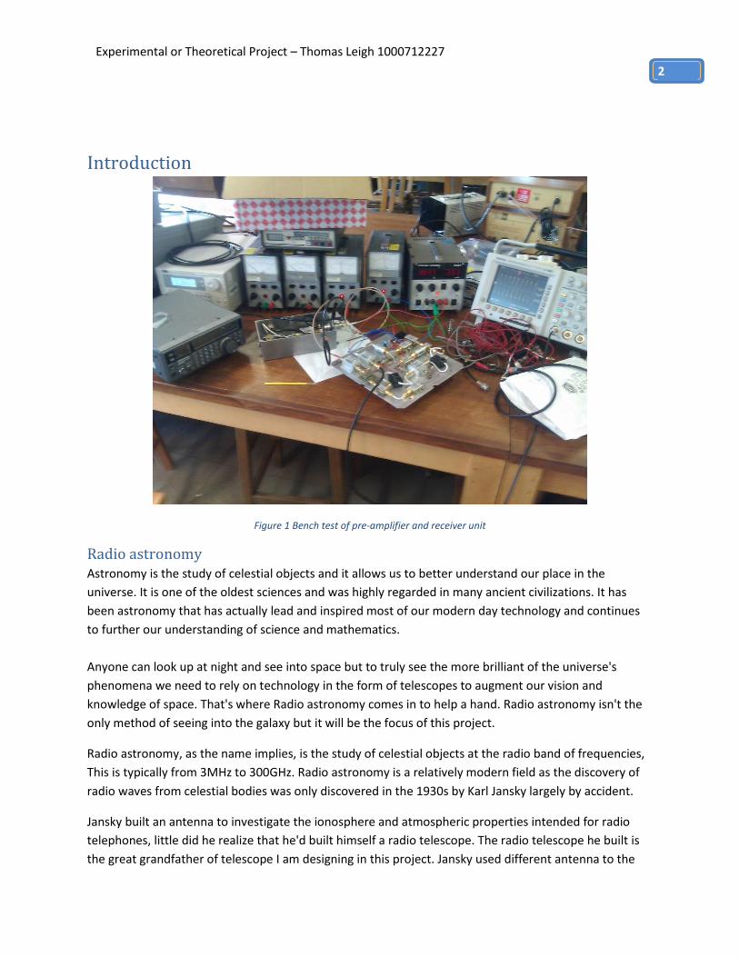
Introduction

Figure 1 Bench test of pre-amplifier and receiver unit

Radio astronomy Astronomy is the study of celestial objects and it allows us to better understand our place in the

universe. It is one of the oldest sciences and was highly regarded in many ancient civilizations. It has

been astronomy that has actually lead and inspired most of our modern day technology and continues

to further our understanding of science and mathematics.

Anyone can look up at night and see into space but to truly see the more brilliant of the universe's

phenomena we need to rely on technology in the form of telescopes to augment our vision and

knowledge of space. That's where Radio astronomy comes in to help a hand. Radio astronomy isn't the

only method of seeing into the galaxy but it will be the focus of this project.

Radio astronomy, as the name implies, is the study of celestial objects at the radio band of frequencies,

This is typically from 3MHz to 300GHz. Radio astronomy is a relatively modern field as the discovery of

radio waves from celestial bodies was only discovered in the 1930s by Karl Jansky largely by accident.

Jansky built an antenna to investigate the ionosphere and atmospheric properties intended for radio

telephones, little did he realize that he'd built himself a radio telescope. The radio telescope he built is

the great grandfather of telescope I am designing in this project. Jansky used different antenna to the


3

ones in this project but the concept is still the same: an antenna, receiver unit and data recorder (for

him this was pen-and-paper). The project will use better equipment then back then but the results will

be much the same.

At 408MHz the most brilliant radio sources are:

Table 1 408MHz brilliance table, comparing the brightest radio sources at 408MHz

Source Identification RA(2000) Dec(2000) Flux Density(f.u.)

Sun Star Varies Varies >250000

Cassiopeia A Supernova Remnant 23h 23.4m 58°49' 4500

Cygnus A Radio Galaxy 19h 59.5m 40°44' 4000

Taurus A Supernova Remnant 05h 34.5m 22°01' 1250

Virgo A Radio Galaxy 12h 30.8m 12°23' 450

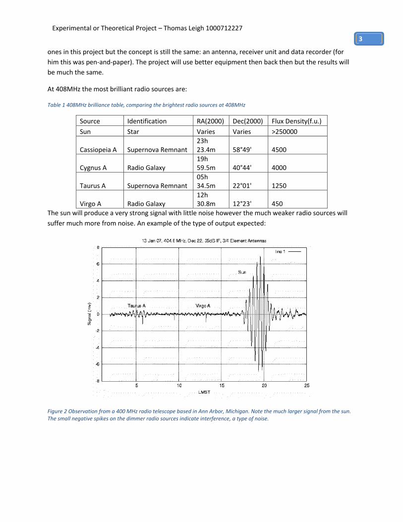
The sun will produce a very strong signal with little noise however the much weaker radio sources will

suffer much more from noise. An example of the type of output expected:

Figure 2 Observation from a 400 MHz radio telescope based in Ann Arbor, Michigan. Note the much larger signal from the sun. The small negative spikes on the dimmer radio sources indicate interference, a type of noise.


4

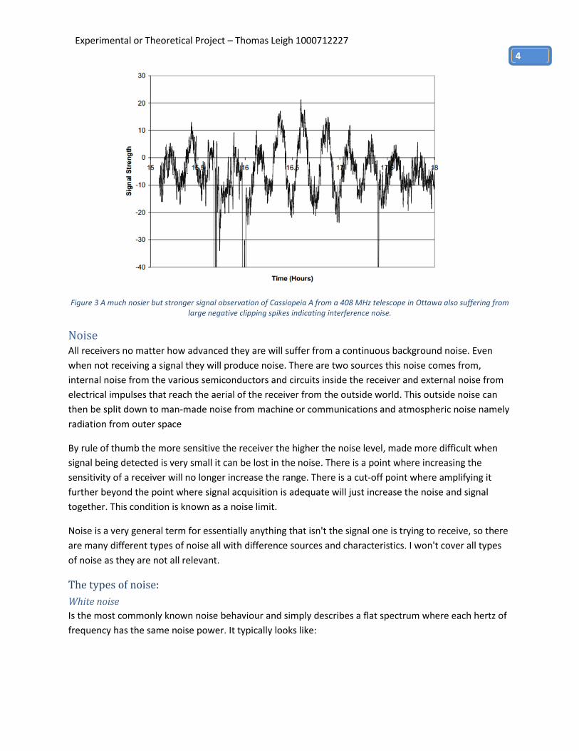
Figure 3 A much nosier but stronger signal observation of Cassiopeia A from a 408 MHz telescope in Ottawa also suffering from large negative clipping spikes indicating interference noise.

Noise All receivers no matter how advanced they are will suffer from a continuous background noise. Even

when not receiving a signal they will produce noise. There are two sources this noise comes from,

internal noise from the various semiconductors and circuits inside the receiver and external noise from

electrical impulses that reach the aerial of the receiver from the outside world. This outside noise can

then be split down to man-made noise from machine or communications and atmospheric noise namely

radiation from outer space

By rule of thumb the more sensitive the receiver the higher the noise level, made more difficult when

signal being detected is very small it can be lost in the noise. There is a point where increasing the

sensitivity of a receiver will no longer increase the range. There is a cut-off point where amplifying it

further beyond the point where signal acquisition is adequate will just increase the noise and signal

together. This condition is known as a noise limit.

Noise is a very general term for essentially anything that isn't the signal one is trying to receive, so there

are many different types of noise all with difference sources and characteristics. I won't cover all types

of noise as they are not all relevant.

The types of noise:

White noise

Is the most commonly known noise behaviour and simply describes a flat spectrum where each hertz of

frequency has the same noise power. It typically looks like:


5

Figure 4 A white noise spectrum of intensity verses frequency.

Internal noise

The main way to discern internal noise from external noise is by unplugging the aerial and checking to

see if one's noise level persists. Assuming that no component one uses in a receiver is faulty or has

faulty wiring the main sources of internal noise are: Thermal noise, shot noise and flicker noise.

Thermal noise

Thermal noise or also ‘Johnson noise’ is typically behaves as white noise and produced by the random

motion of charge carriers in conductors.

Electrons in a conductor are in constant motion and that motion increases proportionally to the

temperature of that conductor. The voltage produced by those electrons add together like alternating

current voltages (the square of the sum of squares). Adding two conductors of the same resistance

joined in series their sum noise voltage produced is root two times what it would be singularly.

𝑉 𝑛𝑜𝑖𝑠𝑒(𝑅𝑀𝑆) = (4𝑘𝑇𝑅𝐵)1/2

Where K is Boltzmann's constant T is the temperature in kelvin, R is the resistance of the conductor and

B is the bandwidth in Hertz. As this type of noise is so closely related to the temperature of a device it is

always present. A draconian solution to reducing this type of noise is to immerse one's receiver in liquid

nitrogen.


6

Figure 5 Shows the relationship between Thermal noise voltages against resistance (National Semiconductor Corp.)

The amplitude of this type of noise is impossible to predict as it in its nature manifests itself as chaotic

particle motion (Brownian motion). It does however follow a Gaussian distribution:

Figure 6 Shows noise voltage RMS (Vn), where p(V) dV is the probability that instantaneous voltage is between V and V + dV.

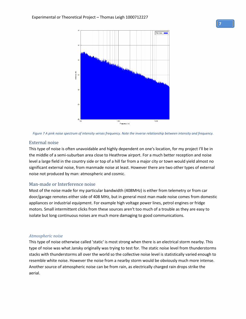
Flicker noise (1/f)

Otherwise known as 'pink noise' in amplifying devices give an additional source of noise at low

frequencies. This follows an inverse proportionality to noise power with respect to one over frequency.

This type of noise is present in all devices like semiconductors, even at high frequencies (albeit much

smaller). It is a result of short comings of the materials used to make them or imperfections in

fabrication. It typically looks like:


7

Figure 7 A pink noise spectrum of intensity verses frequency. Note the inverse relationship between intensity and frequency.

External noise

This type of noise is often unavoidable and highly dependent on one's location, for my project I'll be in

the middle of a semi-suburban area close to Heathrow airport. For a much better reception and noise

level a large field in the country side or top of a hill far from a major city or town would yield almost no

significant external noise, from manmade noise at least. However there are two other types of external

noise not produced by man: atmospheric and cosmic.

Man-made or Interference noise

Most of the noise made for my particular bandwidth (408MHz) is either from telemetry or from car

door/garage remotes either side of 408 MHz, but in general most man made noise comes from domestic

appliances or industrial equipment. For example high voltage power lines, petrol engines or fridge

motors. Small intermittent clicks from these sources aren't too much of a trouble as they are easy to

isolate but long continuous noises are much more damaging to good communications.

Atmospheric noise

This type of noise otherwise called 'static' is most strong when there is an electrical storm nearby. This

type of noise was what Jansky originally was trying to test for. The static noise level from thunderstorms

stacks with thunderstorms all over the world so the collective noise level is statistically varied enough to

resemble white noise. However the noise from a nearby storm would be obviously much more intense.

Another source of atmospheric noise can be from rain, as electrically charged rain drops strike the

aerial.


8

Cosmic noise

Quite a bit of noise is received from the Milky Way and other galaxies as radiation. While the ionosphere

protects us from some of this radiation, it is transparent as certain wavelengths and not only changes

from day to night due to changes in density and therefore refractive index.

Signal-to-noise ratio (SNR)

Signal to noise ratio is simply the noise root mean square (RMS) against the signal RMS to the input

defined by

Equation 1 Signal to noise ratio in decibels

𝑆𝑁𝑅 = 10𝑙𝑜𝑔10 (𝑉𝑠

2

𝑉𝑛2) 𝑑𝐵

Where Vs is the RMS of the signal voltage and Vn is the RMS of the noise voltage. This will be given at a

particular bandwidth and centre frequency as the SNR will drop significantly as the bandwidth is

increased.

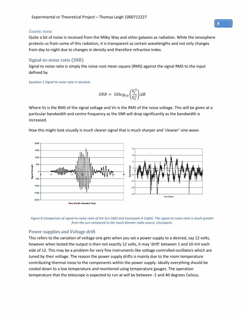
How this might look visually is much clearer signal that is much sharper and ‘cleaner’ sine wave:

Figure 8 Comparison of signal-to-noise ratio of the Sun (left) and Cassiopeia A (right). The signal-to-noise ratio is much greater from the sun compared to the much dimmer radio source, Cassiopeia.

Power supplies and Voltage drift

This refers to the variation of voltage one gets when you set a power supply to a desired, say 12 volts,

however when tested the output is then not exactly 12 volts, it may 'drift' between 1 and 10 mV each

side of 12. This may be a problem for very fine instruments like voltage controlled oscillators which are

tuned by their voltage. The reason the power supply drifts is mainly due to the room temperature

contributing thermal noise to the components within the power supply. Ideally everything should be

cooled down to a low temperature and monitored using temperature gauges. The operation

temperature that the telescope is expected to run at will be between -1 and 40 degrees Celsius.


9

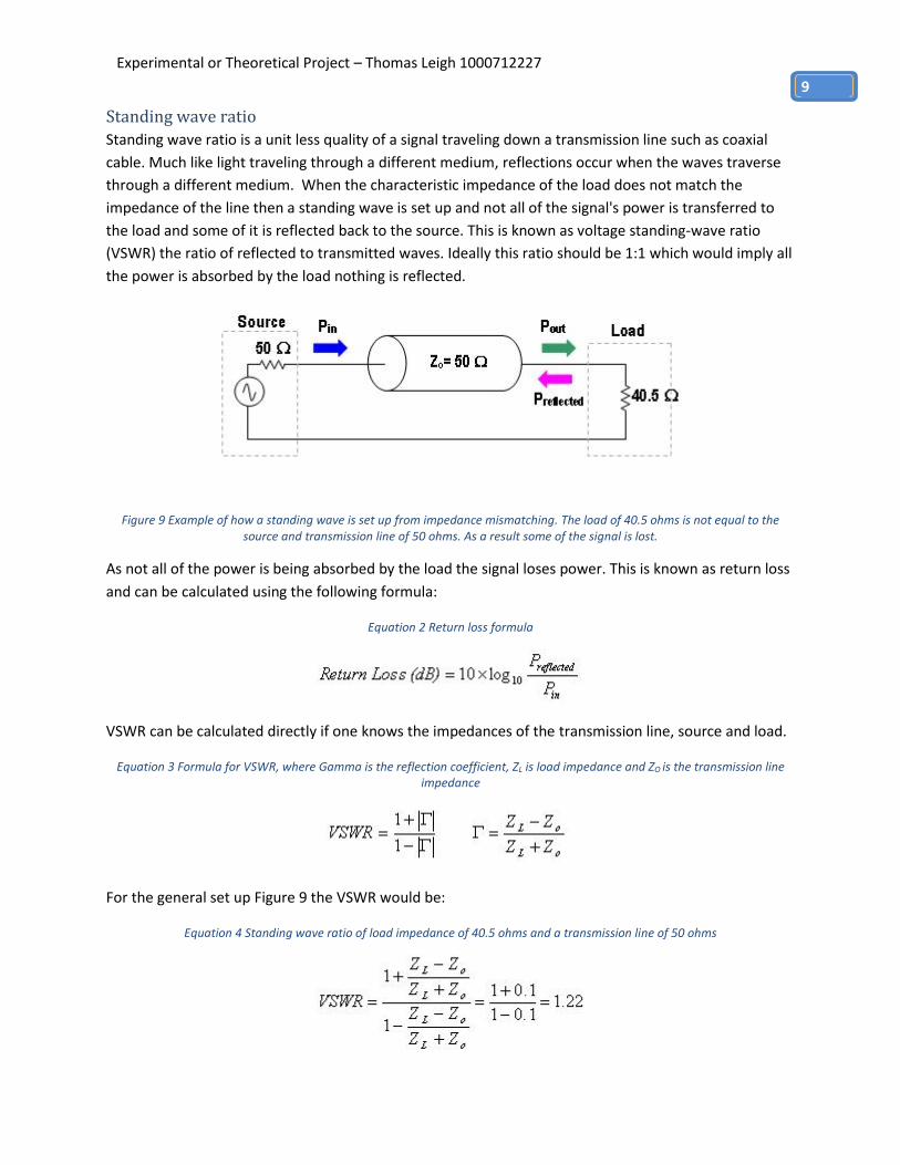
Standing wave ratio

Standing wave ratio is a unit less quality of a signal traveling down a transmission line such as coaxial

cable. Much like light traveling through a different medium, reflections occur when the waves traverse

through a different medium. When the characteristic impedance of the load does not match the

impedance of the line then a standing wave is set up and not all of the signal's power is transferred to

the load and some of it is reflected back to the source. This is known as voltage standing-wave ratio

(VSWR) the ratio of reflected to transmitted waves. Ideally this ratio should be 1:1 which would imply all

the power is absorbed by the load nothing is reflected.

Figure 9 Example of how a standing wave is set up from impedance mismatching. The load of 40.5 ohms is not equal to the source and transmission line of 50 ohms. As a result some of the signal is lost.

As not all of the power is being absorbed by the load the signal loses power. This is known as return loss

and can be calculated using the following formula:

Equation 2 Return loss formula

VSWR can be calculated directly if one knows the impedances of the transmission line, source and load.

Equation 3 Formula for VSWR, where Gamma is the reflection coefficient, ZL is load impedance and ZO is the transmission line impedance

For the general set up Figure 9 the VSWR would be:

Equation 4 Standing wave ratio of load impedance of 40.5 ohms and a transmission line of 50 ohms


10

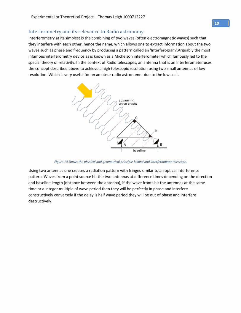
Interferometry and its relevance to Radio astronomy Interferometry at its simplest is the combining of two waves (often electromagnetic waves) such that

they interfere with each other, hence the name, which allows one to extract information about the two

waves such as phase and frequency by producing a pattern called an 'Interferogram'.Arguably the most

infamous interferometry device as is known as a Michelson interferometer which famously led to the

special theory of relativity. In the context of Radio telescopes, an antenna that is an Interferometer uses

the concept described above to achieve a high telescopic resolution using two small antennas of low

resolution. Which is very useful for an amateur radio astronomer due to the low cost.

Figure 10 Shows the physical and geometrical principle behind and interferometer telescope.

Using two antennas one creates a radiation pattern with fringes similar to an optical interference

pattern. Waves from a point source hit the two antennas at difference times depending on the direction

and baseline length (distance between the antenna), if the wave fronts hit the antennas at the same

time or a integer multiple of wave period then they will be perfectly in phase and interfere

constructively conversely if the delay is half wave period they will be out of phase and interfere

destructively.


11

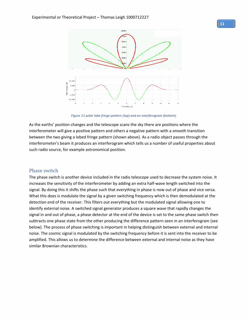
Figure 11 polar lobe fringe pattern (top) and an interferogram (bottom)

As the earths’ position changes and the telescope scans the sky there are positions where the

interferometer will give a positive pattern and others a negative pattern with a smooth transition

between the two giving a lobed fringe pattern (shown above). As a radio object passes through the

interferometer's beam it produces an interferogram which tells us a number of useful properties about

such radio source, for example astronomical position.

Phase switch The phase switch is another device included in the radio telescope used to decrease the system noise. It

increases the sensitivity of the interferometer by adding an extra half-wave length switched into the

signal. By doing this it shifts the phase such that everything in phase is now out of phase and vice versa.

What this does is modulate the signal by a given switching frequency which is then demodulated at the

detection end of the receiver. This filters out everything but the modulated signal allowing one to

identify external noise. A switched signal generator produces a square wave that rapidly changes the

signal in and out of phase, a phase detector at the end of the device is set to the same phase switch then

subtracts one phase state from the other producing the difference pattern seen in an interferogram (see

below). The process of phase switching is important in helping distinguish between external and internal

noise. The cosmic signal is modulated by the switching frequency before it is sent into the receiver to be

amplified. This allows us to determine the difference between external and internal noise as they have

similar Brownian characteristics.


12

Figure 12 An example of the two states of the phase switch (0/320 degrees and 180 degrees) and their resulting difference pattern in an interfeogram


13

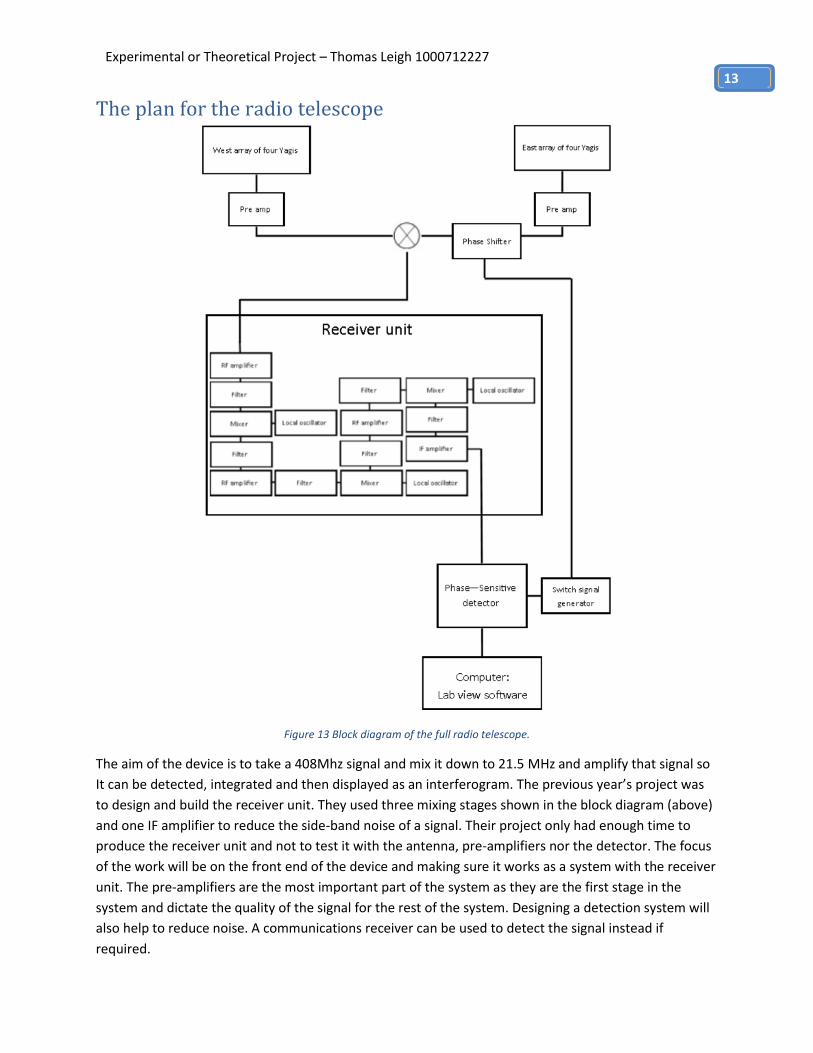
The plan for the radio telescope

Figure 13 Block diagram of the full radio telescope.

The aim of the device is to take a 408Mhz signal and mix it down to 21.5 MHz and amplify that signal so

It can be detected, integrated and then displayed as an interferogram. The previous year’s project was

to design and build the receiver unit. They used three mixing stages shown in the block diagram (above)

and one IF amplifier to reduce the side-band noise of a signal. Their project only had enough time to

produce the receiver unit and not to test it with the antenna, pre-amplifiers nor the detector. The focus

of the work will be on the front end of the device and making sure it works as a system with the receiver

unit. The pre-amplifiers are the most important part of the system as they are the first stage in the

system and dictate the quality of the signal for the rest of the system. Designing a detection system will

also help to reduce noise. A communications receiver can be used to detect the signal instead if

required.


14

Testing the previous year’s receiver I needed to make sure that the receiver last year’s project still correctly amplified at 408 MHz, doing this

required testing the input voltage and checking the receiver with an oscilloscope and test signal.

The experimental equipment was set up like so:

Figure 14 A test signal of 10 mV and varying frequency was used to find the largest amplitude gain on the oscilloscope, the multi-meters were attached to each of the oscillators output to check for consistency.

I used a multi-meter to check each mixing stage’s oscillator then waited to make sure they stabilized.

Table 2 The voltages of first, second and third mixing stages over four hours from powering the voltage regulator on the device.

Voltage (volts) mili

amps hours

first Second Third current time

9.64 4.16 11.14 3.92 0

9.62 4.16 11.12 3.93 2

9.62 4.16 11.12 3.94 4

Table 3 Oscillator voltages, power supply current, elapsed time after turn on and peak frequency of receiver unit

Voltage (volts) mili amps hours MHz

first second third current time frequency

9.7 4.18 11.22 3.93 0 405.4

9.63 4.15 11.15 3.93 0.49 408.2

9.63 4.15 11.14 3.92 1.03 408.1

9.62 4.15 11.14 3.93 1.51 407.9

9.62 4.16 11.12 3.94 2.86 408


15

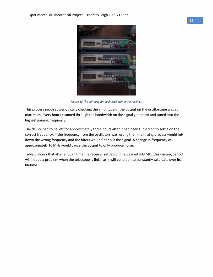
Figure 15 The voltages for each oscillator in the receiver.

This process required periodically checking the amplitude of the output on the oscilloscope was at

maximum. Every hour I scanned through the bandwidth on the signal generator and tuned into the

highest gaining frequency.

The device had to be left for approximately three hours after it had been turned on to settle on the

correct frequency. If the frequency from the oscillators was wrong then the mixing process would mix

down the wrong frequency and the filters would filter out the signal. A change in frequency of

approximately 10 MHz would cause the output to only produce noise.

Table 3 shows that after enough time the receiver settled on the desired 408 MHz this waiting period

will not be a problem when the telescope is finish as it will be left on to constantly take data over its

lifetime.


16

Designing the phasing harness

Yagis discussion

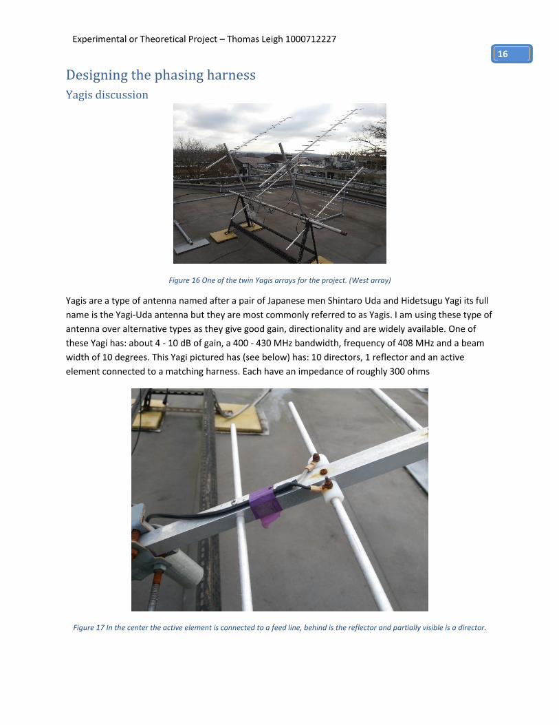
Figure 16 One of the twin Yagis arrays for the project. (West array)

Yagis are a type of antenna named after a pair of Japanese men Shintaro Uda and Hidetsugu Yagi its full

name is the Yagi-Uda antenna but they are most commonly referred to as Yagis. I am using these type of

antenna over alternative types as they give good gain, directionality and are widely available. One of

these Yagi has: about 4 - 10 dB of gain, a 400 - 430 MHz bandwidth, frequency of 408 MHz and a beam

width of 10 degrees. This Yagi pictured has (see below) has: 10 directors, 1 reflector and an active

element connected to a matching harness. Each have an impedance of roughly 300 ohms

Figure 17 In the center the active element is connected to a feed line, behind is the reflector and partially visible is a director.


17

A Yagi will have an active element which is effectively a simple dipole to which the coaxial cable is

attached, also known as the 'driven antenna'. The Driven element is the only part of the Yagi that is

attached to the feed line. The other metal bars known as 'directors' are required to change the shape of

the radiation pattern (See below) and increase the gain of the antenna in a certain direction. The metal

bar behind and slightly larger than the driven element called a 'reflector' this is to minimize the back

lobes on the radiation pattern otherwise this would contribute undesired noise. Any element on a Yagi

that aren't electronically connected to the feed line are known as 'parasitic elements' they work by

acting as passive resonator cancelling out waves in certain directions like the reflector and combining

waves in other directions like the directors.

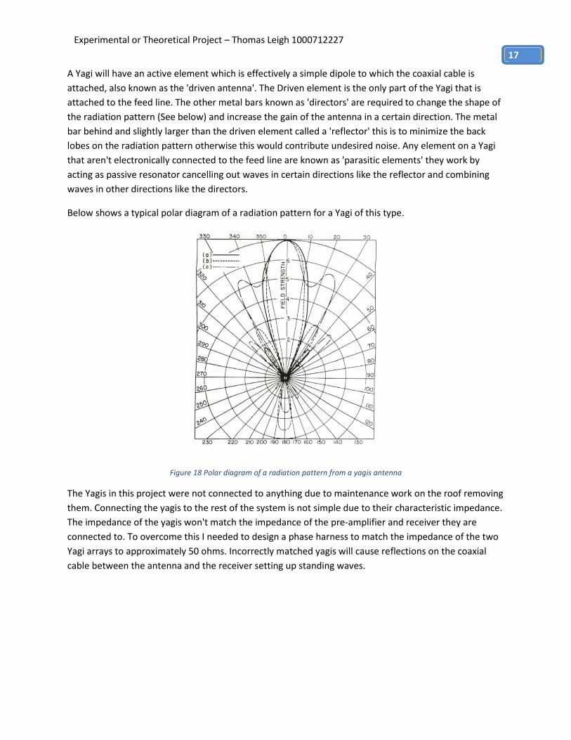
Below shows a typical polar diagram of a radiation pattern for a Yagi of this type.

Figure 18 Polar diagram of a radiation pattern from a yagis antenna

The Yagis in this project were not connected to anything due to maintenance work on the roof removing

them. Connecting the yagis to the rest of the system is not simple due to their characteristic impedance.

The impedance of the yagis won't match the impedance of the pre-amplifier and receiver they are

connected to. To overcome this I needed to design a phase harness to match the impedance of the two

Yagi arrays to approximately 50 ohms. Incorrectly matched yagis will cause reflections on the coaxial

cable between the antenna and the receiver setting up standing waves.


18

Figure 19 Matching harness for matching the impedance of two yagis antenna down to 75 ohms

Using the template above, I adapted it to match four Yagis to 50 ohms:

Figure 20 Hand drawn adaptation of the figure above to match four antenna instead of two.

Designing the phasing harness simply required applying the concept in the template three times. One

for each pair in the array. Then another stage for both pairs. However for the final stage I removed the

75 ohm coaxial termination as the quarter wavelength segment comfortably combines the 75 Ohm

inputs from yagis A to D to 51 ohms. This is an acceptable impedance for the receiver device.


19

Designing pre-amplifiers

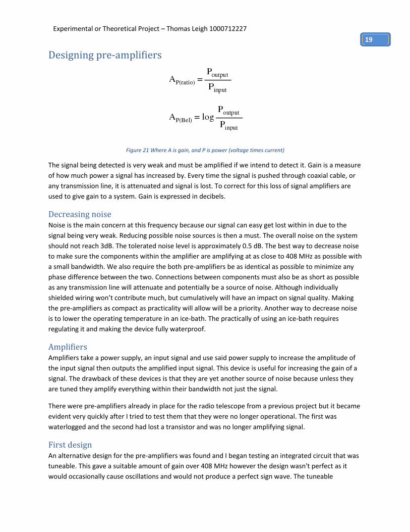
Figure 21 Where A is gain, and P is power (voltage times current)

The signal being detected is very weak and must be amplified if we intend to detect it. Gain is a measure

of how much power a signal has increased by. Every time the signal is pushed through coaxial cable, or

any transmission line, it is attenuated and signal is lost. To correct for this loss of signal amplifiers are

used to give gain to a system. Gain is expressed in decibels.

Decreasing noise Noise is the main concern at this frequency because our signal can easy get lost within in due to the

signal being very weak. Reducing possible noise sources is then a must. The overall noise on the system

should not reach 3dB. The tolerated noise level is approximately 0.5 dB. The best way to decrease noise

to make sure the components within the amplifier are amplifying at as close to 408 MHz as possible with

a small bandwidth. We also require the both pre-amplifiers be as identical as possible to minimize any

phase difference between the two. Connections between components must also be as short as possible

as any transmission line will attenuate and potentially be a source of noise. Although individually

shielded wiring won’t contribute much, but cumulatively will have an impact on signal quality. Making

the pre-amplifiers as compact as practicality will allow will be a priority. Another way to decrease noise

is to lower the operating temperature in an ice-bath. The practically of using an ice-bath requires

regulating it and making the device fully waterproof.

Amplifiers Amplifiers take a power supply, an input signal and use said power supply to increase the amplitude of

the input signal then outputs the amplified input signal. This device is useful for increasing the gain of a

signal. The drawback of these devices is that they are yet another source of noise because unless they

are tuned they amplify everything within their bandwidth not just the signal.

There were pre-amplifiers already in place for the radio telescope from a previous project but it became

evident very quickly after I tried to test them that they were no longer operational. The first was

waterlogged and the second had lost a transistor and was no longer amplifying signal.

First design An alternative design for the pre-amplifiers was found and I began testing an integrated circuit that was

tuneable. This gave a suitable amount of gain over 408 MHz however the design wasn't perfect as it

would occasionally cause oscillations and would not produce a perfect sign wave. The tuneable


20

capacitors on the circuit board were changed to correct the oscillating and after two attempts the circuit

board pre-amplifier was getting better gains and not oscillating. This design became unusable as two

identical versions were required to match phase and producing a second copy with an identical

frequency was difficult. I eventually decided that they weren't worth spending any more time on. This

design proved that a tuneable pre-amplifier produces the best gain.

Tuneable amplifier 1

peak frequency Input voltage (mili volts) Pk-Pk Voltage (mili volts) Gain

408 MHz 10 mV 178 mV 17.8

Testing to find the best gain on the first amplifier design (without oscillations)

Figure 22 The first pre amplifier design with tunable capacitors.

Second design Going back to the original pre-amplifiers, found in the old pre-amplifier box, I saw they contained a

circuit board and a large cavity with a screw that allowed for tuning. As it turned out after replacing a

transistor in the circuitry one of them still worked. When I tested this amplifier on its own it didn't give

as much gain as the previous design but it did however have a very narrow and very accurate bandwidth

around 408 MHz which was perfect for reducing noise into the system.

Testing the cavity amp it gave notably less gain then the tunable amplifier however it was not as prone

to oscillations then the first design.

Cavity amp


408 MHz 10 mV 35 mV 3.5


21

Figure 23 second design, resonance cavity pre-amplifier with circuit still inside.

Fortunately there was still a prototype cavity amplifier in storage meaning we had two identical cavity

amplifiers which is exactly what I needed.

The gain on the cavity amplifiers was still relatively small though so I considered using the first amplifier

design in tandem with the cavity.

Cavity amp plus first design amplifier in series


408 MHz 10 mV 360 mV 36

Although this gave a good gain at a narrow bandwidth it still had the problem that I didn't have two

identical versions of the first design however it did prove that using an extra preamplifier in series with

the cavity was the best option.

Third design Finally we found a spare 'minicircuits' amplifier, the small metal rectangle pictured below, which we

initially thought to be broken when I was testing different devices. My supervisor managed to fix it by

replacing a semi-conductor on the circuit board inside. Using this with the cavity gave a high gain and we

had two of them.

Cavity amp plus Minicircuits amp in series 400-420 MHz bandwith



22

408 MHz 10 mV 76 mV 7.6

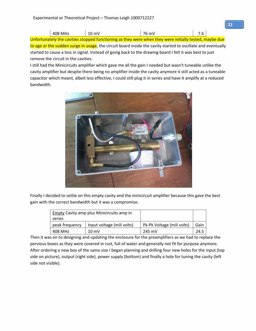
Unfortunately the cavities stopped functioning as they were when they were initially tested, maybe due

to age or the sudden surge in usage, the circuit board inside the cavity started to oscillate and eventually

started to cause a loss in signal. Instead of going back to the drawing board I felt it was best to just

remove the circuit in the cavities.

I still had the Minicircuits amplifier which gave me all the gain I needed but wasn't tuneable unlike the

cavity amplifier but despite there being no amplifier inside the cavity anymore it still acted as a tuneable

capacitor which meant, albeit less effective, I could still plug it in series and have it amplify at a reduced

bandwidth.

Finally I decided to settle on this empty cavity and the minicircuit amplifier because this gave the best

gain with the correct bandwidth but it was a compromise.

Empty Cavity amp plus Minicircuits amp in series


408 MHz 10 mV 245 mV 24.5

Then it was on to designing and updating the enclosure for the preamplifiers as we had to replace the

pervious boxes as they were covered in rust, full of water and generally not fit for purpose anymore.

After ordering a new box of the same size I began planning and drilling four new holes for the input (top

side on picture), output (right side), power supply (bottom) and finally a hole for tuning the cavity (left

side not visible).


23

Below is the first template I used for designing the box for the preamplifier initially I had the input on

the bottom side but then realized this would be impractical given the length of cabling I had so moved it

to the other side of the box. I also neglected to account for the power supply which I later amended. My

supervisor then pointed out it would be advantageous to put in a hole for tuning the cavity after it was

set up as the capacitance would not be the same when finally plugged in on the roof compared to

testing it on the bench in the lab. Lining up the cavity to the hole was particularly tricky and I had to use

blue-tac, many rulers and a pen marker to make sure I could get a screwdriver through the hole to the

screw in the cavity. In the end I did manage it and it is possible to reach the screw in the cavity but the

hole was slightly off about a centimeter which made me appreciate how difficult it is measuring and

engineering something that requires very fine dimensions.

Testing the system

The Signal generator problem When initially learning about man made noise and amplifiers my supervisor was showing me a radio

receiver and demonstrating what noise sounds like. It gave me an appreciation for how intrusive and

how abundant it was, scanning through anything from 300 MHz all the way up to 2000 MHz one could

find many intelligent and random signals, some of them extremely strong.

I was testing the radio receiver curiously tuning into any signal I could find while I waited for oscillators

in the receiver I mentioned earlier to settle. When suddenly to my utter dismay I found a signal on 408

MHz using the radio receiver (which was located on the roof). I was quite surprised because I was led to

understand by my supervisor that 408 MHz was a frequency reserved for radio astronomy and the signal

I was getting was around 20 dB. After spending roughly half an hour to an hour trying to figure out what

was causing this signal (and panicking) I went back to my testing the receiver and turned it off satisfied it

was working correctly. When I went to check the radio again the mysterious signal had completely

disappeared.

What had happened was the signal generator was not properly shielded and was radiating its generated

408 MHz signal I’d been using to test the receiver all around the room and to the radio antenna on the

roof. Turned out the mysterious signal swamping my reserved frequency was myself!

After explaining my accidental blunder to my supervisor he then demonstrated that if one puts a 400 Hz

modulation on the signal generator one can play a tone on the radio. Which meant to my utter


24

amusement I could play a simple tune or transmit a Morse code messages by repeatedly turning the

signal generator on and off.

Conclusion What I gathered from this project was a thorough understanding of electronics and an appreciation for

elegance and complexity of signal processing. After having the opportunity to play with the amplifiers

and simple integrated circuits it really increased my confidence with not only building electronic for the

telescope but even simple domestic electronics. I found myself trying to fix Ethernet cables and rewiring

plugs that I would have never even attempted prior to this project.

I also have an appreciation for the nature of radio waves and how antennas work seeing detailed polar

diagrams of different antenna how even putting one’s hand through a simple dipole connected to the

signal generator effects the power of the received signal gave me a very visceral understanding of how

delicate and prone to noise they can be.

Which brings me on to the nightmare that is noise a bane to every amateur radio astronomer especially

when one lives in a built up area close to a major city, at the time of writing I was living in Egham of

Surrey, even worse when a major airport is close by. Noise for me was pretty much unavoidable but if I

ever got the opportunity later in life to build my own radio telescope I would love to find some clean

open rural location where noise was almost nonexistent.

I really enjoyed building the radio telescope, it felt nice to work towards something tangible and useful.

All too often University assignments tend to be self-fulfilling, learning for the sake of learning, but this

project gave me a sense of learning while I was doing. Doing a project to build something gives a great

context to the skills I gained to which I will never forget.

Future projects.


25


26

Appendix

The oscilloscope: The oscilloscope used is a 5 GS/s, 400MHz, 50 ohm TDS 3044B and requires a BNC connector.

Figure 24 An example oscilloscope output, shown is output through a preamplifier and coaxial cable

Signal generator The signal generator is a 2GHz RF sine wave generator and requires an N-type connector. The signal

generator was not properly shielded and would leak radio waves around the room as I found out in my

testing.

Figure 25 The signal generator left used to test the bandwidth of a filter.


27

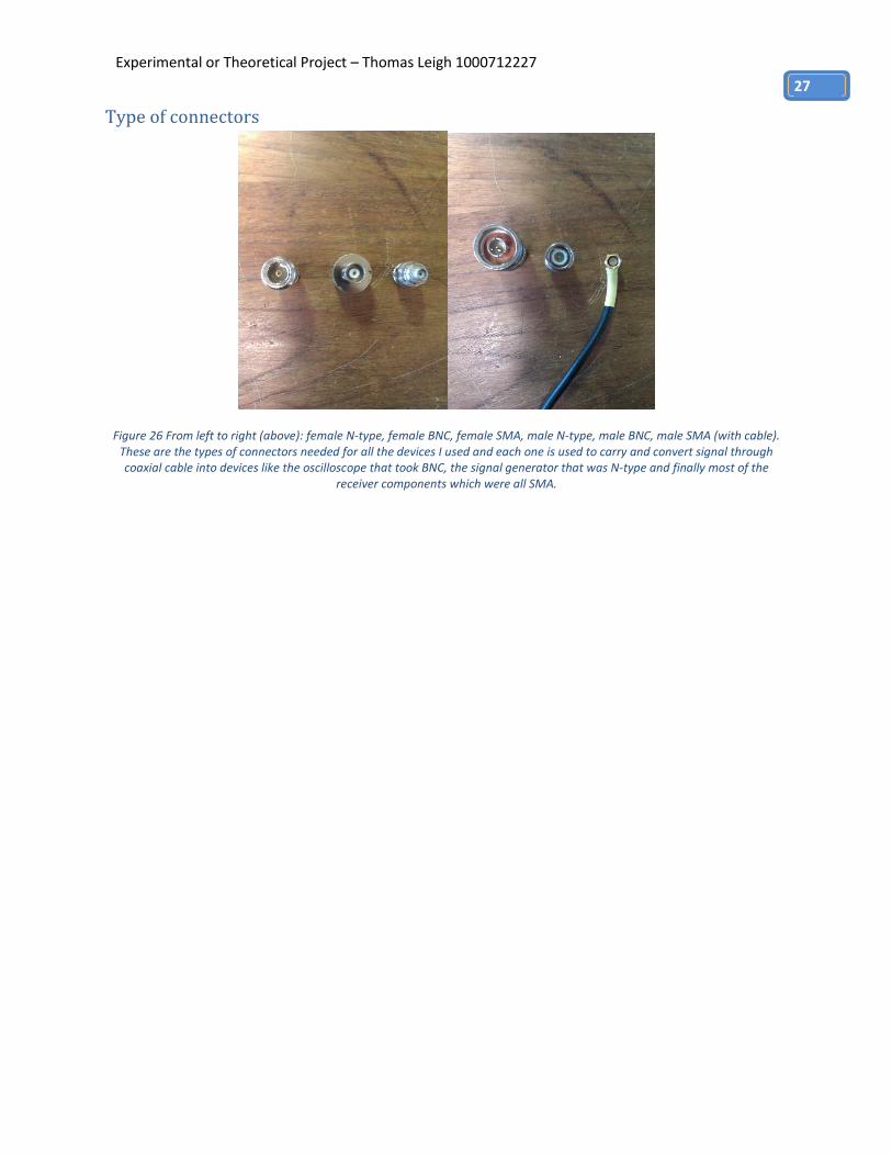
Type of connectors

Figure 26 From left to right (above): female N-type, female BNC, female SMA, male N-type, male BNC, male SMA (with cable). These are the types of connectors needed for all the devices I used and each one is used to carry and convert signal through coaxial cable into devices like the oscilloscope that took BNC, the signal generator that was N-type and finally most of the

receiver components which were all SMA.


28

References [Needs expanding!]

yagi polar diagram

R. M. Fishenden and E. R. Wiblin: "Design of Yagi Aerials," Proc. IEE (London), pt. III, vol. 96 p. 6, January,

1949.

interferometer

http://www.radioastronomy.me.uk/html/interferometry.html

interferogram

http://fringes.org/ra101_fr.html

Radio hand book

Horowitz and hill

Antenna engineering handbook – Jasik

TO DO LIST:

contents

coaxial cable

future projects

picture legends

detailed Refferences

http://fringes.org/ra101_fr.html

Bsc Project MASTER

Documents

Transcript of Bsc Project MASTER