Brownian dynamics simulations of bead-rod and bead-spring...

J. Non-Newtonian Fluid Mech. 108 (2002) 227–255

Brownian dynamics simulations of bead-rod and bead-springchains: numerical algorithms and coarse-graining issues

Madan Somasia, Bamin Khomamia,∗, Nathanael J. Woob,Joe S. Hurc, Eric S.G. Shaqfehc

a Department of Chemical Engineering and Materials Research Laboratory, Washington University,Campus Box 1198, St. Louis, MO 63130, USA

b Scientific Computing/Computational Mathematics Program, Stanford University, Stanford, CA 9305, USAc Department of Chemical and Mechanical Engineering, Stanford University, Stanford, CA 9305, USA

Received 6 August 2001; received in revised form 10 October 2001

Abstract

The efficiency and robustness of various numerical schemes have been evaluated by performing Brownian dynam-ics simulations of bead-rod and three popular nonlinear bead-spring chain models in uniaxial extension and simpleshear flow. The bead-spring models include finitely extensible nonlinear elastic (FENE) springs, worm-like chain(WLC) springs, and Pade approximation to the inverse Langevin function (ILC) springs. For the bead-spring chainstwo new predictor–corrector algorithms are proposed, which are much superior to commonly used explicit and otherfully implicit schemes. In the case of bead-rod chain models, the mid-point algorithm of Liu [J. Chem. Phys. 90(1989) 5826] is found to be computationally more efficient than a fully implicit Newton’s method. Furthermore,the accuracy and computational efficiency of two different stress expressions for the bead-rod chains, namely theKramers–Kirkwood and the modified Giesekus have been evaluated under both transient and steady conditions. Itis demonstrated that the Kramers–Kirkwood with stochastic filtering is the preferred choice for transient flow whilethe Giesekus expression is better suited for steady state calculations. The issue of coarse graining from a bead-rodchain to a bead-spring chain has also been investigated. Though bead-spring chains are shown to capture onlysemi-quantitatively the response of the bead-rod chains in transient flows, a systematic coarse-graining procedurethat provides the best description of bead-rod chains via bead-spring chains is presented.© 2002 Elsevier Science B.V. All rights reserved.

Keywords: Brownian dynamics; Dilute polymer solution; Bead-spring model; Bead-rod model; Shear flow; Extensional flow;Algorithm; Coarse graining

∗ Corresponding author. Tel.:+1-314-935-6065; fax:+1-314-935-7211.E-mail address: [email protected] (B. Khomami).

0377-0257/02/$ – see front matter © 2002 Elsevier Science B.V. All rights reserved.PII: S0377-0257(02)00132-5

228 M. Somasi et al. / J. Non-Newtonian Fluid Mech. 108 (2002) 227–255

1. Introduction

Quantitative predictions of the velocity and stress distributions in complex flows of polymeric solutionsis a challenging goal, but offers the promise of more rational design of polymer processing operations.The conventional approach to modeling the flow of dilute polymeric solutions is based on solving theequations of conservation of mass, momentum and energy in conjunction with a closed-form constitutiveequation for the polymeric stress (e.g.[1–3]). To date, the most commonly used closed-form constitutiveequations for dilute polymeric solutions have been obtained by approximating models based on kinetictheory. However, such approximations commonly referred to as ‘closure approximations’ often distortthe predictions of the original kinetic theory based model[4].

In recent years, continuum level discretization techniques have been successfully merged with Brow-nian dynamics (BD) techniques to allow direct use of micro-structural models for polymer dynamics inflow simulations, thus by-passing the need for closed-form constitutive equations[5–8]. Algorithms forefficient continuum/mesoscopic simulation have advanced at a rapid rate since their first introduction inthe early 90s. However, even with the most efficient multi-scale algorithms, complex flow simulationshave been limited to include only very simple micro-structural models for the polymeric molecule, suchas the elastic dumbbell model. This is due to the fact that this class of simulations is very CPU inten-sive primarily due to the large ensemble required to obtain accurate polymeric stresses from Browniandynamic simulations. Hence, use of more complex micro-structural models such as bead-rod chains incomplex flow simulations is beyond the reach of the current computing power.

In order to improve the efficiency and predictive capability of combined mesoscopic/continuum sim-ulation techniques, two issues need to be addressed. First, more CPU efficient BD algorithms need to bedeveloped. Secondly, accurate coarse-graining procedures from a molecular level (i.e. atomistic) to meso-scopic level (e.g. bead-rod and bead-spring chains) need to be developed. In what follows, we will brieflydescribe the basic approach in coarse graining from an atomistic to a mesoscopic level of description.

The coarse graining from an atomistic level to the bead-rod description is based on sound statisticalmechanic principles. Specifically, atomic vibrations are neglected leading to ‘freely rotating bonds’.Moreover, the distance between the adjacent beads, i.e. the ‘Kuhn step’ can be determined based on thefact that pair-wise inter-atomic potential interactions can be neglected beyond a certain distance. Furthercoarse graining from a bead-rod to a bead-spring chain relies on the assumption of local equilibratedmotion of many Kuhn steps. Hence, a number of Kuhn steps are replaced by a ‘phantom entropic spring’.It should be noted that depending on the flow strength, the number of Kuhn steps that can be equivalentlyreplaced by an entropic spring is different; hence systematic coarse-graining procedures from the bead-rodto the bead-spring chains are rarely available. Finally, in the most coarse-grained approximation, one canneglect the internal structure of the molecule and represent the whole molecule as a single dumbbell withan entropic spring. However, an alternative procedure has been suggested by Ghosh et al.[9] who haverecently proposed a coarse-graining procedure based on an adaptive length scale principle, where theproperties of the entropic spring are adjusted based on the flow strength.

As mentioned earlier, flow simulations of dilute polymeric solutions with micromechanical modelscontaining sufficient molecular level information to describe the nonlinear rheology of polymeric solu-tions, require fast BD algorithms as well as the need for accurate coarse-graining procedures. Hence, wehave focused our attention on the development of CPU efficient BD simulation algorithms for bead-rodand bead-spring chains as well as the development of a rational coarse-graining procedure to repre-sent a bead-rod chain by a smaller bead-spring chain. Specifically, we have compared the performance

M. Somasi et al. / J. Non-Newtonian Fluid Mech. 108 (2002) 227–255 229

of a fully implicit Newton’s method against the commonly used two-step mid-point technique for BDsimulation of bead-rod chains. In addition, the accuracy and CPU efficiency of thestochastically fil-tered Kramers–Kirkwood and the modified Giesekus expressions for evaluating the polymeric stress inbead-rod simulations have been compared.

Similarly, for the bead-spring models the performance of conventional explicit techniques with a fullyimplicit technique based on Newton’s method have been examined. In addition, two new predictor–corrector based techniques are introduced. Continued iteration of these methods results in fully self-consistent methods and their performance relative to the other two techniques is discussed. Finally,coarse graining from a bead-rod to a bead-spring chain is examined. The aim is to find the numberof Kuhn steps that can be replaced by an equivalent nonlinear entropic spring such that the polymericstress computed from both micro-structural models are equivalent over a wide range of flow types andWeissenberg numbers.

The manuscript is organized as follows. The governing equations and the expressions for the stresstensor for various nonlinear bead-spring chains and the Kramers chains are introduced inSection 2.Following this, the various numerical methods used to solve the governing equations for both bead-rodand bead-spring models are discussed. The two new algorithms for flow simulation of the three differentbead-spring chains are introduced in this section. The relative performance of the various numericaltechniques discussed inSection 2is also examined inSection 3. Specifically, the accuracy of the solutionand the computational efficiencies of the various techniques are examined. This is followed by thediscussion of the scaling relationships and coarse-graining procedures inSection 4. We conclude byhighlighting the best simulation algorithms.

2. Governing equations

In the following, a brief description of the governing equations for the two micro-structural models,namely the bead-rod chain and the bead-spring chain necessary to evaluate the chain dynamics underflow will be discussed.

The bead-rod chain consists ofNk beads connected byNk −1 rigid rods of lengtha (Fig. 1). The beadsserve as interaction points with the solvent and the massless rods act as rigid constraints in the chain thatkeep every bead at a constant distancea away from its neighboring beads.

Fig. 1. The freely jointed bead-rod chain (Kramers chain) model for a polymer chain.


The governing equations for the dynamics of the chain are obtained by summing the external forcesacting on the beads,

F Hi + F C

i + F Bi = 0, i = 1,2, . . . , Nk (1)

where the subscripti refers to the bead number andF H, F C, F B are the hydrodynamic drag force, theconstraint force and the Brownian force, respectively. The hydrodynamic force is the Stokes drag actingon the beads in the absence of hydrodynamic interaction and fluid inertia and is simply given by,

F Hi = −ζ(r i − u∞

i ) (2)

whereζ is the drag coefficient (i.e. the drag tensor has been assumed to be isotropic),r i the velocity of thebead andu∞

i is the solvent velocity at beadi. The constraint force is the force that keeps two neighboringbeads at a constant distancea away from each other, and can be written in terms of the tensionsTi in therods as follows,

F Ci = Tiui − Ti−1ui−1 (3)

whereui = (r i+1 − r i)/a is the orientation of rodi connecting beadsi andi + 1 with position vectorsr i

andr i+1, respectively. The Brownian force is used to represent the frequent collisions between the beadand the solvent molecules and is mathematically represented as a quantity with zero mean (because of theisotropic nature of the collisions) and a second moment that balances the dissipative forces (also knownas the fluctuation–dissipation theorem of the second kind[11]). Therefore,F B is chosen such that

〈F Bi (t)〉 = 0 (4)

〈F Bi (t)F

Bj (t + �t)〉 = 2kTζ δijδ(�t) ≈ 2kTζ δij

�t(5)

wherek is the Boltzmann’s constant,T the absolute temperature,δij the Dirac delta andδ is the unittensor. In the above equations,〈· · · 〉 represents an ensemble average.

After substitution of different forces acting on the beads intoEq. (1)and rearranging, one can obtainthe following set of equations governing the evolution of the position vectors of the beads:

dr i =[u∞i + F C

i

ζ

]dt +

√2kT

ζdW i , i = 1,2, . . . , Nk (6)

where dW i is a Wiener process mathematically represented by a Gaussian random number with a meanof zero and variance dt. The above set of equations have to be solved subject to the constraints that thedistance of separation between any two adjacent beads at any instant of time is fixed ata, or

(r i+1 − r i) · (r i+1 − r i) − a2 = φ2, i = 1,2, . . . , Nk − 1 (7)

whereφ2 is a specified tolerance (typically 10−6 to 10−8).Eqs. (6) and (7)result in 2Nk−1 equations forNk

position variablesr i andNk −1 tensionsTi , which can be solved in a number of ways. In the next section,two numerical schemes, namely the Newton’s method and the method of Lagrange multipliers will bediscussed. To facilitate comparison with the bead-spring results, we have chosen to non-dimensionalizethe above equations as follows. The distance between adjacent beadsa serves as the length scale of theproblem, the bead diffusion time,ζa2/kT serves as the characteristic time scale and the forces are madedimensionless withkT/a.


Once the position vectors of all the beads have been determined, the polymer contribution to the totalstress,τ p can be obtained using the Kramers–Kirkwood expression (neglecting the isotropic contribution)as,

τp =Nk∑i=1

〈RiFHi 〉 (8)

whereRi is the position of beadi relative to the center of mass of the chain, i.e.,

Ri = r i − rc (9)

where

rc = 1

Nk

Nk∑i=1

r i . (10)

In Eq. (8)the polymer stressτ p has been non-dimensionalized usingnpkT, with np being the numberdensity of the polymers in solution. Furthermore, in order to obtain smooth averages, we have followed thenoise reduction technique proposed by Doyle et al.[10]. In addition to the Kramers–Kirkwood expressiondiscussed above, the polymer stress can also be obtained using the modified Giesekus expression as givenby [11,12]

τp = −1

2

[Nk∑i=1

〈RiRi〉](1)

(11)

where the superscript (1) denotes the upper convected derivative,

X(1) = ∂X

∂t− Pe(κ† · X + X · κ) (12)

wherePe = γ (ζa2/kT) is the bead Peclet number, which can be interpreted as the ratio of the beaddiffusion time to the characteristic flow time.

Although the modified Giesekus expression for the polymer stress is more useful in evaluating thepolymeric stress under steady state conditions, we have chosen to evaluate its usefulness in transientflows as well, since it is simpler to evaluate than the Kramers–Kirkwood expression with the noisereduction technique of Doyle et al.[10].

2.1. Simulation procedure

The initial conditions for the positions vectors of each bead in a chain are obtained by simulating arandom walk, i.e. each successiver i+1 − r i is obtained by invoking a random unit vector on a surface ofa sphere. The first bead is assumed to be at the origin, which thus specifies the remaining position vectorsuniquely. However, since it is known that, at equilibrium, a Kramers chain does not exactly follow a randomwalk structure[12], the correct initial distribution is obtained by allowing all the chains to equilibrate fora significant time period (typically 106–107 time steps, which corresponds to around 1000 times the beaddiffusion time). Once the correct equilibrium distribution has been obtained, the chains are subject to flowat timet = 0, after which,Eq. (6) is integrated in time subject to the constraints and any macroscopic


properties such as the stress are obtained via appropriate averages. Typically, 1000–4000 chains are usedin every transient simulation, with time steps of 10−3 to 10−5 depending on the flow strength.

2.2. Bead-spring chains

A bead-spring chain consists ofM beads connected byNs = M − 1 entropic springs. While the beadsserve as interaction points with the solvent, the springs represent entropic effects due to the internaldegrees of freedom which have been lost in the process of coarse graining. The governing equations areobtained as before by summing the external forces acting on the beads

F Hi + F E

i + F Bi = 0, i = 1,2, . . . ,M (13)

where the subscripti refers to the bead number andF H, F E, F B are the hydrodynamic drag force, theeffective spring force and the Brownian force, respectively.

The expressions for the hydrodynamic force (i.e.Eq. (2)) and the Brownian force (Eqs. (4) and (5)) areidentical to the corresponding bead-rod chain expressions. The effective spring force on beadi is givenas

F Ei =

F s1 if i = 1

F si − F s

i−1 if 1 < i < M

F sM−1 if i = M

(14)

whereF si is the spring force associated with springi. Depending on the force law used for the springs, one

can arrive at different models. In this work, we shall make use of three widely used nonlinear spring forcelaws to model the springs, i.e. the finitely extensible nonlinear elastic (FENE) force law, the worm-likechain (WLC) force law[13] and a Pade approximation to the inverse Langevin force law (ILC)[14]. Theforce laws are summarized below for comparison:

F FENEi = HsQi

1 − Q2/Q20

(15)

F WLCi = kT

bK

[1

2

1

(1 − (Q/Q0))2− 1

2+ 2Q

Q0

]Qi

Q0(16)

F ILCi = kT

bK

Qi

Q0

[3 − (Q/Q0)

2

1 − (Q/Q0)2

](17)

whereQi = r i+1 − r i is the connector vector of theith spring,Hs the spring constant,Q the magnitudeof Qi andQ0 is the maximum extensibility of each spring. InEq. (16)we have used the fact that theKuhn lengthbK is twice the persistence lengthlp, i.e.bK = 2lp. Lastly, we note that all spring force lawsin Eqs. (15)–(17)follow the Hookean spring force law in the small deformation limit.

Eq. (13)can be rearranged to obtain the stochastic differential equation (SDE) governing the evolutionof the position vectors of the beads of the bead-spring chain as

dr i =[u∞i + F E

i

ζ

]dt +

√2kT

ζdW i , i = 1,2, . . . ,M (18)


Furthermore, the polymer stress,τ p, is given by the Kramers expression as follows

τp =Ns∑i=1

〈QiFsi〉 (19)

To begin the simulations, typically 1000–10,000 chains are chosen which satisfy the equilibrium dis-tribution function of a bead-spring chain comprised of Hookean springs. As in our bead-rod simulations,these chains are allowed to equilibrate for 104–106 steps such that the correct distribution for a givenforce law is obtained. The flow field is then introduced and the evolution of the chains is monitored.Furthermore, macroscopic properties such as the viscosity and its first normal stress coefficient are ob-tained at any time through appropriate averaging. In order to facilitate comparisons with the bead-rodsimulations, it is important to introduce the characteristic scales for non-dimensionalization. The averageequilibrium length of a Hookean dumbbell,

√kT/Hs, has been chosen as the length scale in the simula-

tions. Time is made dimensionless byζ /4Hs (i.e. the relaxation time of a Hookean dumbbell), and stress isnon-dimensionalized withnpkT as before. We define the Weissenberg number as the product of the longestrelaxation time (λ) and the shear rate (γ ). For bead-rod chains,We = λγ = 0.0142N2

k γ (ξka2/kT). Sim-

ilarly for bead-spring chains,We = λdγ = λdγ (ξ/4Hs). The detail of how the longest relaxation timesfor both bead-rod and bead-spring chains are calculated from the simulation is outlined inSection 4.3.For both chains,We is the product of the dimensionless longest relaxation time andPe. The dimensionlessform of the equations and the numerical techniques used to solve them are introduced in the next section.

3. Numerical techniques

To compare the accuracy and CPU efficiency of various techniques, simulations have been performedin two homogeneous flows, namely the start-up of steady shear and uniaxial extensional flow. In the caseof steady shear flow, the velocity field is given as

vx = γ y; vy = vz = 0 (20)

and for uniaxial extensional flow, the velocity field takes the form

vx = εx; vy = −12 εy; vz = −1

2 εz (21)

whereγ andε are the shear rate and elongation rate, respectively.

3.1. Bead-rod simulations

In the following, the integration scheme and subsequently, the solvers used for the bead-rod simulationsare described. We have used the iterative technique originally proposed by Liu[15] to solve the SDEsdescribing the evolution of the bead position vectorsr i , which, when written in the dimensionless formare as follows

dr i = [Pe(κ · r i) + F Ci ]dt +

√2 dW i , i = 1,2, . . . , Nk (22)

subject to the constraint

(r i+1 − r i) · (r i+1 − r i) − 1 = φ2, i = 1,2, . . . , Nk − 1 (23)


whereκ = ∇v† is the transpose of the velocity gradient tensor. Since the above equations have beenrendered dimensionless,κ has the form

κ =

0 1 0

0 0 0

0 0 0

; κ =

1 0 0

0 −12 0

0 0 −12

(24)

in simple shear and extensional flow, respectively.In Liu’s [15] approach, givenr i(t), r i(t +δt) is obtained utilizing a predictor–corrector type algorithm.

The predictor step consists of an ‘unconstrained’ move (i.e.F Ci = 0) such that,

r∗i = r i(t) + Peκ(t) · r i(t)dt +

√2 dW i , i = 1,2, . . . , Nk (25)

Following this,r i(t + δt) is obtained as

r i(t + δt) = r∗i + F C

i δt (26)

CombiningEqs. (23) and (26), along with the expression for the constraint forceF Ci from Eq. (3)gives

Nk − 1 nonlinear equations for the tensionsTi ,

(2δt)bi · (Ti−1ui−1 − 2Tiui + Ti+1ui+1) + (Ti−1ui−1 − 2Tiui + Ti+1ui+1)2(δt)2

= φ2 + 1 − (|bi |)2, i = 1,2, . . . , Nk (27)

wherebi = r∗i+1 − r∗

1. The above set of nonlinear equations can be solved using a number of differentapproaches, and in this study we shall examine a few methods. The first method is a Picard’s method,which is identical to that used by Liu[15]. The nonlinear terms in tensions (second term on the left-handside) appearing in the above equation are assumed to be small in comparison to the linear terms. Therefore,the set of equations is rewritten in terms of a linear set of equations and solved iteratively by evaluating thenonlinear part from the previous iteration. This results in a tridiagonal system of equations for theNk −1tensions. Alternatively, Newton’s method can be used to solve the set of discrete equations. UtilizingNewton’s method,Eq. (27)can be rewritten as,

F i(x)≡ (2δt)bi · (Ti−1ui−1 − 2Tiui + Ti+1ui+1) + (Ti−1ui−1 − 2Tiui + Ti+1ui+1)2(δt)2 − φ2 − 1

+ (|bi |)2 = 0, i = 1,2, . . . , Nk − 1 (28)

whereF i is theith equation and we definex = {T1, T2, . . . , TNk−1}† as the vector of the tension variables.To implement this technique we note that given the value ofx = xold at any instant, the value ofx = xnew

at the next iteration can be obtained according to Newton’s method as

xnew = xold − J−1(xold) · F (xold) (29)

whereJ−1 is the inverse of the Jacobian matrixJ defined as

J = ∂F

∂x(30)

whereF = {F1, F2, . . . , FNk−1}†. The process is repeated until|xnew − xold| < tolerance, where thetolerance is typically 10−6 to 10−8.


Both the methods outlined above need an initial condition forx. Usually, the solution at the previoustime step is taken to be the starting guess for the iterative process at the present time. It should be notedthat, while the convergence rate of the Newton’s method is quadratic, as opposed to the linear convergenceof the Picard’s method, Newton’s method involves evaluating the Jacobian atevery iteration, while theresulting tridiagonal matrix of the linear Picard’s method is constant for all iterations at any particulartime step. The relative performance of both these methods for different chain lengths and for various flowstrengths will be discussed below.

3.2. Bead-spring simulations

In this section we illustrate all algorithms only for the case of FENE chains realizing that extensions toother nonlinear bead-spring cases can be similarly accomplished. Since the spring forces can be writtenin terms of the inter-bead displacements, it will be useful to write the SDEs describing the bead-springchain dynamics in terms of the connector vectorsQi rather than the bead positionsr i

dQi = [Pe(κ · Qi) + 14(F

si−1 − 2F s

i + F si+1)]δt +

√12(dW i+1 − dW i) (31)

for i = 1,2, . . . , Ns. The above equation has been written in the dimensionless form utilizing the scalesintroduced inSection 2. For example, the dimensionless spring forceF s

i for a FENE dumbbell has theform

F si = Qi

1 − Q2i /b

(32)

whereb = HsQ20/kT is the dimensionless extensibility parameter. The other spring force laws inEqs. (16)

and (17)can be made dimensionless using the same scalings outlined inSection 2.2.Eq. (31)can again be integrated utilizing various techniques. The simplest procedure involves march-

ing forward in time using an explicit forward Euler integration scheme. The next improvement to thistechnique is the Picard’s method, in which the explicit solution procedure is iterated at every time stepuntil the residual of the solution falls below a pre-specified tolerance. However, when using these explicittechniques, care should be taken that the length of the connector vectorQ does not exceed the maxi-mum permissible value

√b, because this would result in aphysical spring forces. This can be avoided

by following the rejection algorithm proposed by Öttinger[11], i.e. a move that results in an aphysicalspring force law is rejected. Alternately, one can use Newton’s method to solve the set of nonlinearequations iteratively at every time step until convergence is achieved. Furthermore, the resulting set oflinear equations at every iteration in the Newton’s method within a time step can be either solved usinga direct solver, or an iterative solver.

In this work, we shall compare both the explicit methods and the fully implicit Newton’s method totwo new semi-implicit predictor–corrector methods that we have developed to integrate the above set ofequations. These methods, which have been motivated by the two-step semi-implicit method proposedby Öttinger (to integrate a FENE dumbbell)[11] are given below. Note that in each of these methodswe can and do continue the predictor–corrector iteration to convergence. Thus these techniques can beconsidered to bealternative fully implicit solution techniques as they produce self-consistent solutions ateach time step.

In the first algorithm, given the solutionQni at timet = nδt , the solutionQn+1

i at the next time stept = (n + 1)δt , is obtained as follows:


Step 1. In the predictor step,Qi(tn) is explicitly updated to obtainQ∗i (tn) as

Q∗i = Qn

i + [Pe(κ · Qni ) + 1

4(Fs,ni−1 − 2F

s,ni + F

s,ni+1)]δt +

√12(dW n

i+1 − dW ni ) (33)

whereFs,ni is the spring force for theith segment at timet = nδt .

Step 2. In the first corrector step, the spring forces for segmentsi andi − 1 are treated implicitly whensolving forQi such that

Qi + 12(δt)F

si = Qn

i + [ 12Pe(κ · Qn

i + κ · Q∗i ) + 1

4(Fsi−1 + F

s,ni+1)]δt +

√12(dW n

i+1 − dW ni ) (34)

which, upon rearrangement, results in the following cubic equation for the magnitude ofQi for eachithspring in the chain

|Qi |3 − R|Qi |2 − b(1 + 12(δt))|Qi | + b × R = 0 (35)

whereR is the magnitude of the right-hand side vector ofEq. (34)andb is the dimensionless extensibilityparameter. This equation has one unique root between 0 and

√b, and thus by choosing this root, we can

ensure that|Qi | is never greater than√b.

Step 3. In the final corrector step, once again the spring forces for segmentsi and i − 1 are treatedimplicitly, while the spring force for segmenti + 1 is obtained from Step 2.

Qn+1i + 1

2(δt)Fs,n+1i = Qn

i + [ 12Pe(κ · Qn

i + κ · Qi) + 14(F

s,n+1i−1 + F s

i+1)]δt

+√

12(dW n

i+1 − dW ni ) (36)

The above equation also results in a cubic equation similar toEq. (35), which can be solved to obtaina root for|Qi | that lies between 0 and

√b. Once everyQn+1

i is known, the residualε is calculated as the

difference between the solutionsQi andQn+1i .

ε =√√√√ Ns∑

i=1

(Qn+1i − Qi)

2 (37)

If this residual is greater than a specified tolerance (e.g. 10−6), Qn+1i is copied ontoQi and Step 3 is

repeated until convergence. This results in a self-consistent semi-implicit method. Basically, the premiseof the new method lies in the fact that, the force law,F

si for any spring in the chain, is either written

explicitly (from the previous time step or from a previous step in the present time step, where the lengthof the connector is guaranteed to be within the bounds) or solved implicitly through the cubic equation.This ensures that no Brownian step is rejected at any time during the entire simulation.

For the WLC and inverse Langevin chain, we obtain a different cubic equation thanEq. (35)above. Asin the FENE case, we are still guaranteed a unique real root between 0 and

√b.

We have also investigated a second slightly different algorithm which treats the spring force term usinga trapezoidal rule instead of the backward Euler scheme as inEqs. (34) and (36). In this case the overallalgorithm becomes second order accurate because the trapezoidal rule is a higher order scheme. However,


in actuality, there is no improvement in accuracy due to the discontinuities in the Brownian forcing term[16]. For this algorithm the corrector steps corresponding toEqs. (34) and (36)are given by

Qi + 14(δt)F

si = Qn

i + [ 12Pe(κ · Qn

i + κ · Q∗i ) + 1

8(Fsi−1 + F

s,ni+1) + 1

8(Fs,ni−1 − 2F

s,ni + F

s,ni+1)]δt

+√

12(dW n

i+1 − dW ni ) (38)

Qn+1i + 1

4(δt)Fs,n+1i = Qn

i + [ 12Pe(κ · Qn

i + κ · Qi) + 18(F

s,n+1i−1 + F

si+1)

+ 18(F

s,ni−1 − 2F

s,ni−1 + F

s,ni+1)]δt +

√12(dW n

i+1 − dW ni ) (39)

Similarly we have the following cubic equation for the FENE in the trapezoidal algorithm,

|Qi |3 − R|Qi |2 − b(1 + 14(δt))|Qi | + b × R = 0 (40)

We have found that the performance of these two algorithms is nearly identical. For shear flow, thetrapezoidal algorithm performs better than backward Euler scheme at a very large time step (i.e.�t = 0.1),while for extensional flow the backward Euler scheme outperforms the trapezoidal scheme. For typicaltime steps these two algorithms give identical results, thus in what follows we shall only directly comparethe backward Euler scheme to the explicit and Newton’s implicit schemes.

3.3. Cubic equation iteration schemes

We have also investigated various iteration schemes to solveEqs. (34), (36), (38) and (39). In the contextof a linear matrix equationAx = b, the matrixA can be split into three matricesA = D +L+U , whereD, L andU are the diagonal, lower triangular, and upper triangular matrices, respectively. The simplestiteration scheme known asJacobi method is obtained by retaining the diagonal matrix on the left side ofthe equation while moving the rest of the matrices to the other side resulting inDx = −(L+U)x+b. Thisis motivated by the fact that inverting a diagonal matrix is much more CPU efficient than inverting a moregeneral matrix. Therefore the iteration scheme isxn+1 = D−1(−(L+U)xn +b). The convergence of theiteration scheme depends on the eigenvalues of the matrix−(L + U ). For Gauss–Seidel (GS), we retain(D + L) on the left side of the equation and the iteration scheme becomesxn+1 − (D + L)−1(Uxn + b).Similarly for successive over-relaxation (SOR), we havexn+1(−(1/ωD+L)−1((1−1/ω)D+U)xn+b).The choice of different methods of splitting the matrixA is motivated by a search for the iteration techniquewith the highest convergence rate. For linear matrix problems, with a special choice ofω, SOR can reducethe spectral radius of the iteration matrix and a faster convergence is obtained over Jacobi and GS iterations[17].

A similar approach is followed when solving nonlinear problems. The simplest scheme is Jacobi-likeiteration, whereF

si−1 in Eqs. (34) and (38)are evaluated in the previous iteration step asF

s,ni−1, andF

s,n+1i−1

in Eqs. (36) and (39)are evaluated asFsi−1. Alternatively, one can divide the equations into two groups

based on bead number, oddi’s and eveni’s, and iteratively calculate |Q| in Eqs. (34) and (38)alternatingwith even and oddi values. Since each spring is connected only to its nearest neighbors, the equationsare completely decoupled. This is known as ablack-and-white or two-color GS iteration[17]. Since thisis equivalent to using the most updated values of |Q|s, it is easy to understand why GS converges fasterthan Jacobi iteration. The iteration scheme we presented inEqs. (34), (36), (38) and (39)are identical to


the two-color GS method with the bead numbers merely renumbered in a different order. Similarly wecan try a variant of the SOR method in which a fraction of the non-coupling force term is moved to theother side in addition to the terms moved by the GS method. In the nonlinear problem, we find SOR iseven slower than Jacobi iteration and we find that the GS iteration scheme is about 30–100% faster thanJacobi iteration method. Therefore we have presented results based on the fastest iteration scheme (i.e.the two-color GS as shown inEqs. (34), (36), (38) and (39)).

4. Results and discussions

4.1. Bead-rod chains

Fig. 2shows the comparison of the CPU time ratio between the Newton’s and the Picard’s method forcalculation in uniaxial extensional flow atWe = 1 and 10. We observe that the Picard’s method is alwaysat least 10% faster than the Newton’s method for any given chain size. We have also found this to begenerally true regardless of flow strength and type.

Furthermore, we have tested the relative performance of the two stress expressions, namely the modifiedGiesekus, i.e.Eq. (11)and the Kramers–Kirkwood given byEq. (8)plus the noise reduction techniqueproposed by Doyle et al.[10]. Fig. 3 shows a typical result for start-up of an extensional flow for 1000chains using both stress expressions. As seen from the figure, both the expressions for stress give almostidentical results both in the transient and the steady state regions. Moreover, the CPU time associatedwith evaluation of the stress using both approaches are very similar. However, if one just observesthe steady part of the curve (Fig. 3(b)), it is obvious that the Giesekus expression outperforms theKramers–Kirkwood expression, especially in regards to the statistical noise associated with the stochasticsimulations. In addition, the Giesekus expression is much simpler to evaluate than the Kramers–Kirkwood

Fig. 2. The ratio of the CPU time for the Newton’s method to the Picard’s iterative method for a 50 bead Kramers chain forWe = 1 and 10.


Fig. 3. Comparison between the Giesekus and Kramers–Kirkwood stress expressions for Kramers chains (Nk = 50,We = 11.4):evolution ofτ xx with time: (a) transient region and (b) steady state region.

expression (with noise reduction technique of Doyle et al.[10]. However, it should be noted that in transientsimulations, the Giesekus stress expression involves evaluating time derivatives, which is not a trivialexercise because of the rapidly fluctuating results. Hence, the derivatives need to besmoothed. To obtainthe results inFig. 3, the smoothing of the derivatives has been performed based on using a number ofprevious variable values instead of employing just the immediate previous value. The effect of increasingthe number of previous variable values in calculating the time derivative on the overall quality of thesolution is shown inFig. 4, where the evolution of the stressτ xx has been plotted as a function of time.


Fig. 4. Comparison between the Giesekus and Kramers–Kirkwood stress expressions for Kramers chains withNp = 200(Nk = 50,We = 11.4): (a) transient and (b) blow-up of initial transient.

Specifically, the time derivative of any quantityX is evaluated as follows

dX(t)

dt= X(t) − X(t − Np �t)

Np �t(41)

We have used different values ofNp, the number of past values, ranging from 2 to 200 in our derivativecalculations. The results shown inFig. 3correspond to a value of 200. Clearly, by choosing an appropriatesize of past values (in this particular case, around 200 past values), we can see that the solution duringthe transient region of the simulation also improves considerably. Furthermore, we have also observedthat as far as the statistical error is concerned, the Giesekus expression with a smoothed derivative


over 20 past values is very similar to that calculated from the Kramers–Kirkwood expression. Valuesbelow 10 result in very large statistical noise when evaluating the stress utilizing the modified Giesekusexpression. Although increase inNp does smooth out the stochastic noise in the derivative calculations,it also introduces a numerical error, proportional to�t, because of the backward difference involved.Therefore, there will always be some value ofNp, beyond which the numerical error more than offsetsthe effects of smoothing out the stochastic noise in the calculations. However, since the�t used in thebead-rod simulations are typically very small, the value ofNp = 20 suggested here should work wellfor most calculations. Moreover, it should be pointed out that use of the modified Giesekus expressionwith smoothing of the derivative could be very memory intensive in a complex flow situation whereone might need to store the values of all stress components at every node for 20 time steps. Therefore acombination of both techniques might be an optimal method that one could use in complex flow situations,i.e. Kramers–Kirkwood with noise reduction procedure of Doyle et al.[10] during strong transients andmodified Giesekus for steady and nearly steady flows.

4.2. Bead-spring chains

Fig. 5 depicts the CPU time ratio between the explicit method and either of semi-implicit predictor–corrector techniques proposed in this study for different FENE chain lengths. The test flow is start-up ofsimple shear flow atWe = 10 and we iterate the predictor–corrector method to full convergence. From thefigure, one can observe that the explicit scheme is at least four times faster than the predictor–correctormethod. This can be explained based on the fact that there are at least three sub-steps at each timefor the new method. In addition, except for the predictor step, the remaining steps in the new algo-rithm are semi-implicit steps which are more computationally intensive than an explicit step. Finally, thenew scheme also involves iterations at each time step to ensure convergence, which requires additionalCPU time.

Fig. 5. CPU time ratio for the predictor–corrector and the explicit for FENE chain simulations of different sizes in shear flow atWe = 10.


Fig. 6. Comparison of the predictor–corrector and explicit methods for four segment FENE chains in extensional flow atWe = 10:evolution ofτ xx with time. Bottom figure shows comparison after steady state has been achieved.

Fig. 6 shows the comparison (in terms of the solution accuracy) between the explicit and eithersemi-implicit method for a four segment chain in start-up of uniaxial extensional flow atWe = 10for two different time steps, namely dt = 0.0001 and 0.001. It can be observed that, for the smallertime step, both the explicit and the predictor–corrector method give identical results.Table 1shows therelative CPU times corresponding toFig. 6. One can clearly observe that the explicit scheme is almostfour times faster than the predictor–corrector method at any given time step. However, when the time stepis increased to 0.001, we observe that only the predictor–corrector scheme gives the correct transients

Table 1CPU times (s) for the solutions obtained using the predictor–corrector and explicit schemes as shown inFig. 6

�t Predictor–corrector Explicit

0.0001 8077 22550.001 1112 224


and steady value for the stresses. In addition, it can be further observed that the predictor–corrector tech-niques are generally two to three times faster than the explicit method for a given solution accuracy. Theinaccuracy associated with the explicit technique with relatively large time steps is due to the rejection ofmoves that lead to aphysical spring force laws. Hence, over the course of the simulation, these rejectionscould significantly alter the true evolution of the chain dynamics. Although one can use an adaptivetime step to make sure no rejections take place during the simulation, this would increase the number ofcomputations performed at each time step. Hence, the advantages of a single step explicit method thatis highly CPU efficient would be lost. More importantly, in self-consistent complex flow simulations,where the deformation rate could rapidly vary from position to position in the flow domain, the use ofthe predictor–corrector methods is essential as they do not lead to rejections and they can be used withmuch larger time steps. This in turn, minimizes the number of times that the macoscopic conservationlaws have to be solved resulting in even more CPU and memory savings.

The explicit method combined with the Picard iterations ensures self-consistent solutions at each timestep. Hence, larger time steps could be used in the simulations. However, the rejections could still alterthe chain dynamics.Fig. 7 depicts the results obtained using the predictor–corrector method with fullconvergence and the explicit/Picard method for a six-segment FENE chain in the start-up of shear flow.Once again, an order of magnitude smaller time step is required for the explicit/Picard method in orderto reproduce the same accuracy in the results as the predictor–corrector technique. Hence, generallyspeaking, to produce the same quality results the combined explicit/Picard’s method is approximatelythree to four times slower than the predictor–corrector method.

To this point, the superiority of the newly proposed predictor–corrector methods relative to explicitmethods has been demonstrated. Next, we shall focus on the performance of the fully implicit Newton’smethod. Two different variations of the method have been examined. The first is the Newton’s method witha direct solver, wherein the Jacobian matrix is inverted using a direct banded solver at every iteration. Thesecond is an iterative solver, where the resulting linear system of equations is iteratively solvedwithin

Fig. 7. Comparison of the solution obtained using the predictor–corrector method and the implicit Picard’s iterative method forsix segment FENE chain in shear flow (dimensionlessWe = 10).


Fig. 8. The ratio of the CPU run time for Newton’s method using direct and iterative solvers for various FENE chain sizes.

every iteration.Fig. 8 shows the CPU efficiency of the Newton’s method with a direct solver and aniterative solver. Clearly, over the range of chain sizes considered, iterative solvers are much slower ascompared to direct solvers. This is due to the fact that the Jacobian matrix for the nonlinear bead-springchains considered is quite small and hence it is more efficient to invert the matrix in one step rather thaniteratively solving the linear system. However, if a very large number of segments are used (i.e.<100) it ispossible that the iterative solver could be more efficient. However, it should be borne in mind that the wholeidea behind coarse graining is to reduce the degrees of freedom in the problem. Hence, for all practicalchain sizes, the iterative solver is not competitive.Fig. 9 shows the relative CPU times between theNewton’s method (with a direct solver at every iteration) and either of our predictor–corrector algorithmswith iteration to convergence for different chain sizes. It can be seen that the predictor–corrector methodsare at least twice as fast as the Newton’s method for small chain sizes and in fact, the predictor–correctortechnique becomes much more CPU efficient for larger chain sizes. This is expected, because as thechain size increases, the Jacobian matrix is more expensive to compute, and furthermore inverting thelarge matrix also becomes more time consuming. Thus Newton’s method becomes less competitive asthe chain size becomes larger.

In order to make the newly proposed predictor–corrector methods even more CPU efficient, we haveincorporated the idea of a ‘look-up’ table in the algorithm. This idea follows from the fact that, in bothSteps 2 and 3 of our algorithms (i.e.Eqs. (34) and (36), or (38) and (39)) we have to solve a cubic equationfor the length of the connector vector (seeEqs. (35) and (40)). Closer inspection of either cubic equationreveals that, while the coefficient of the linear term is a constant throughout the simulations, the othertwo coefficients (quadratic and constant) are functions of only the magnitudeR of the right-hand sidevector ofEq. (34)or (38). Therefore, one can solve this cubic equation at the beginning of the simulationjust once for different values ofR and store the roots in a look-up table. During the simulation, the rootcan be extracted by performing a linear interpolation from the values in the look-up table.Fig. 10showsa typical plot of the cubic root plotted against the parameterR for a maximum extensibility ofb = 900


Fig. 9. The ratio of the CPU run time for Newton’s method (with a direct solver) and predictor–corrector method for variousFENE chain sizes.

from Eq. (35). From the figure, it is obvious that the linear interpolation should work well, since theroot is a very smooth function of the parameterR. In Fig. 11, the CPU time ratio with and without thelook-up table formulation for the predictor–corrector technique defined byEqs. (36) and (39)is plottedas a function of the chain size forWe = 1.0 and maximum extensibility (of every individual spring inthe chain) of 900. It can be observed that incorporating the look-up table into the algorithm more than

Fig. 10. The cube root for a dimensionless extensibility of 900 as a function of the parameterR, which is the magnitude of theright-hand side ofEq. (35).


Fig. 11. The CPU ratio for runs without and with the use of look-up table for different FENE chain sizes.

doubles the computational efficiency of the BD simulations of the bead-spring chains, and this effect isvirtually independent of the chain size. Since stochastic simulations are usually the most expensive partof all complex micro–macro computations, any improvement in making these simulations faster helpsmake the complex flow problem more tractable.

4.3. Comparison of bead-rod and bead-spring chain models

It is well known that a Kramers chain can both qualitatively and quantitatively capture the behaviorof polymer chains in simple flows[4,10,12]. More recently, a Kramers chain matching the molecu-lar parameters of aλ-DNA molecule has shown excellent agreement with single-molecule microscopyexperiment[18–21]. However, since it is impossible to perform self-consistent simulations with thismicro-structural model in complex flows with present day computing power, it becomes imperative thatone has a coarse-graining recipe to reproduce the predictions of Kramers chains using structurally simplermodels. The models often chosen for this purpose are the bead-spring chains. In order to compare resultsbetween bead-rod and bead-spring models, it is worthwhile first to point out the relationship betweenthe parameters of the two models. The length of a fully stretched Kramers chain is given by (Nk − 1)a.Therefore the maximum extensibility of every spring in the correspondingNs segment bead-spring chainis such that

Ns × Q0 = (Nk − 1)a (42)

Correspondingly, the spring constantHs of an individual spring in the bead-spring chain model isrelated to the bead-rod parameters as[12]

Hs = 3kT

(Nk − 1)a2Ns (43)


Sinceb = HsQ20/kT, this implies thatb can be written in terms of the bead-rod parameters as

bs = 3(Nk − 1)

Ns(44)

Since the length scales in the two models have been fixed, we now turn our attention to the time scalesinvolved in the coarse-graining procedure. We denote the time scale of the FENE chains to bet∗s = ζ/4Hs,and the time scale for bead-rod chains to bet∗k = ζka

2/kT, whereζk is the bead drag coefficient for a beadin the bead-rod chain. We have explored various possibilities for determining the scaling relationshipbetweent∗s and t∗k . For example, one can relate the two by fixing the longest relaxation time for thetwo chains to be the same, i.e. we choose the parameters such that the longest relaxation time becomesindependent of the chain length. This is done as follows. The longest relaxation time of the bead-rod chainhas been determined by Doyle et al.[10] for different chain lengths. Specifically, they have determinedthe longest relaxation time by examining the long time relaxation of the stress and/or the birefringenceof an ensemble of chains starting with initial configuration in which every chain is fully stretched in thez-direction. This is analogous to studying the relaxation after subjecting the chains to uniaxial extensionalflow with Weissenberg numberWe → ∞. By performing the above mentioned analysis, they have giventhe following best fit relation between the longest relaxation timeλ and the chain sizeNk

λ = 0.0142N2k

(ζka

2

kT

)= 0.0142N2

k t∗k (45)

We have followed an analogous procedure with the FENE springs. We start with FENE chains almostfully stretched in thez-direction and follow the time evolution of the stress by letting the chains relaxto equilibrium. Thedimensionless longest relaxation timeλd can then be obtained as−1/slope from thesemi-log plot of stress versus time. Subsequently,t∗s can be related tot∗k by equating the longest relaxationtime, i.e.,

t∗s =(

0.0142N2k

λd

)t∗k (46)

A second approach to relate the two time scales is by equating the time scale characterized by thezero-shear material functions of the bead-spring chains to that of the bead-rod chains. The characteristictime scaleλ0 is defined as the ratio of zero-shear first normal stress coefficient and zero-shear viscosity(λ0 = Ψ1,0/2ηp

0) and it is given by the following equations for bead-rod and FENE chains, respectively[12,22]

λKramers0 = 10N3

k − 12N2k + 35Nk − 12

900Nk

(47)

λFENE0 = 1

60

(bs

bs + 5

) [2N2

s + 7 − 12N2

s + 1

Ns(bs + 7)

]. (48)

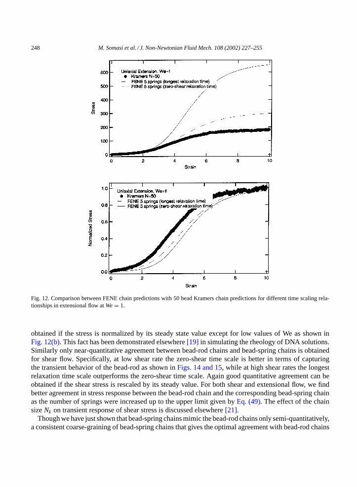
The performance of these time scales have been examined by performing a number of simulations.Overall, we find, for extensional flow, bead-spring chains, with either time scales, fail to quantitativelycapture the transient behavior of the corresponding bead-rod chains (seeFigs. 12 and 13). However, itshould be noted that the scaling based on the longest relaxation time performs better than the zero-sheartime scale for all flow strengths considered. Good agreement between bead-spring and bead-rod can be


Fig. 12. Comparison between FENE chain predictions with 50 bead Kramers chain predictions for different time scaling rela-tionships in extensional flow atWe = 1.

obtained if the stress is normalized by its steady state value except for low values of We as shown inFig. 12(b). This fact has been demonstrated elsewhere[19] in simulating the rheology of DNA solutions.Similarly only near-quantitative agreement between bead-rod chains and bead-spring chains is obtainedfor shear flow. Specifically, at low shear rate the zero-shear time scale is better in terms of capturingthe transient behavior of the bead-rod as shown inFigs. 14 and 15, while at high shear rates the longestrelaxation time scale outperforms the zero-shear time scale. Again good quantitative agreement can beobtained if the shear stress is rescaled by its steady value. For both shear and extensional flow, we findbetter agreement in stress response between the bead-rod chain and the corresponding bead-spring chainas the number of springs were increased up to the upper limit given byEq. (49). The effect of the chainsizeNk on transient response of shear stress is discussed elsewhere[21].

Though we have just shown that bead-spring chains mimic the bead-rod chains only semi-quantitatively,a consistent coarse-graining of bead-spring chains that gives the optimal agreement with bead-rod chains


Fig. 13. Comparison between FENE chain predictions with 50 bead Kramers chain predictions for different time scaling rela-tionships in extensional flow atWe = 50.

can be developed. In the next section we discuss the number of springs in the bead-spring chains neededto best describe bead-rod chains under flow.

4.4. Coarse-graining procedure

Previously Doyle and Shaqfeh[23] compared the bead-rod chain with the FENE-PM and FENE chainin linear flows. They have used the same coarse-graining procedure as ours except that they used theRouse time for their nonlinear bead-spring models instead of the longest relaxation time. As will beshown below, the nonlinear spring force law changes the relaxation time from the linear Rouse time about


Fig. 14. Comparison between FENE chain predictions with 50 bead Kramers chain predictions for different time scaling rela-tionships in shear flow atWe = 10.

30–50% depending on the degree of discretization. Apart from their underestimation ofWe, we find ourmulti-spring FENE results qualitatively consistent with their FENE-PM result. Recently Ghosh et al.[24]proposed similar coarse-graining as ours except they rescaled their relaxation time for the bead-springchain in order to get the same steady state extensional stress as the bead-rod chain. Therefore it is notsurprising that their bead-spring chain result is in better agreement with the bead-rod chain in extensionalflow than the results presented based on the two scalings used in this study. However in shear flow, wehave found the agreement is poor if their scaling is used. Since in a complex flow, the kinematics is neitherpure shear nor pure extensional, their procedure cannot be effectively used in complex flow simulations.

Fig. 15. Comparison between FENE chain predictions with 50 bead Kramers chain predictions for different time scaling rela-tionships in shear flow atWe = 60.


Table 2The longest relaxation time of the worm-like chain with varying number of springs forb = 450

M (number of modes) b = 450

5 1.36910 4.18915 8.74920 14.1230 27.0140 44.58

In order to accurately simulate a polymer chain using the proposed numerical scheme in this paper, weneed systematic criteria for the extent of coarse-graining. In other words, given a number of Kuhn steps(NK) we want to find the minimum number of springs to best capture the behavior of a polymer chain.Previously Doyle et al.[10] found that only Kramers chains consisting of more than 10 rods follow theanalytic inverse Langevin force law. Thus we have the upper bound limit as

Ns ≤ NK

10. (49)

Yet a quantitative criterion for the lower bound on the number of springs is not available. Qualitatively,we have to include as many internal modes as needed to accurately describe the details of the dynamics.Before discussing the coarse-graining procedure, we point out the fact that when a single-spring chain isdiscretized into a multi-spring chain, the force on the chain segments becomes stiffer resulting in higherforce than the single-spring force law. To accommodate this, Hur et al. artificially increased the Kuhnlength size by 45% for their worm-like chain model forλ-DNA [19]. But since the deviation of the forceis a nonlinear function of the chain extensions, a satisfactory rescaling of the force cannot be obtained bysimply adjusting the Kuhn length alone. Also the amount by which the Kuhn length should be increasedcannot be determined unambiguously. Our decision not to rescale the Kuhn length is also based on thereasoning that at small chain extensions, the spring force law should reduce to the Hookean limit withthe correct molecular constants with no adjustable parameters.

First we calculate the longest relaxation time of the worm-like chain discretized into anNs springchain. The relaxation times obtained from birefringence decay are used. We chooseb = 450 whichis the molecular parameter for aλ-DNA molecule[19] andb = 2000 for comparison. The individualextensibility parametersbs are chosen according toEq. (44). The longest relaxation times of the worm-likechain with varyingNs are summarized inTables 2 and 3. AsNs increases, each spring represents a shorterfragment of the molecule, resulting in a stiffer spring. As shown inFig. 16, as we discretize the worm-likechain into a finer grained chain with more springs at a fixed number of Kuhn steps, the deviation of

Table 3The longest relaxation time of the worm-like chain with varying number of springs forb = 2000

M (number of modes) b = 2000

5 1.52920 17.13840 60.79


Fig. 16. The longest relaxation time of the worm-like chain with varying number of springs.

the longest relaxation time from the Rouse relaxation time at the same number of modes (Ns) increases.Moreover, the deviation is more pronounced for smallerbs. We would expect the longest relaxationtimes of the worm-like chain to approach the Rouse limit forbs � 1, however, for smallbs, the longestrelaxation time is considerably different as mentioned in the beginning of this section and should becarefully simulated as discussed inSection 4.3.

To test the convergence of the rheological properties as well as the microscopic properties of chainswith varying numbers of springs, we have performed simulations of aλ-DNA molecule in shear flow. InFig. 17, we have plotted the polymer shear viscosity versus strain in the start-up shear flow forNs = 5,10, 15 and 40 atWe = 60. A qualitative and quantitative difference is observed forM > 15 orM < 5.

Fig. 17. The transient shear viscosity of the worm-like chain with varying number of springs atWe = 60.


Fig. 18. The transient normal stress difference (τ11 − τ22) of the worm-like chain with varying number of springs in shear flowat We = 60.

Based onEq. (49)a worm-like chain of 15 springs would be an adequate coarse-grained model for aλ-DNA molecule and the prediction is in agreement with the simulation result shown inFig. 17. Thenormal stress difference in the start-up of shear flow is shown for varying number of springs inFig. 18and again we see a significant deviation for chains with more than 15 springs.

Based on these results, we conclude thatNs = 15 is the number of springs necessary to mimic thebehavior of aλ-DNA molecule. Though we have based our discussion of coarse-graining on a particularspring model (worm-like chain), the same procedure applies to other spring laws such as FENE chainand inverse Langevin chain.

5. Conclusions

In this study, we have considered two issues related to molecular simulations of viscoelastic flowswith prescribed kinematics employing bead-rod and bead-spring chain models. First, various numericalschemes used to simulate such models have been investigated in terms of their solution accuracy and CPUtimes. Secondly, the issue of coarse graining from the expensive bead-rod chains to simpler bead-springchains has been examined.

Specifically, the relative performance of two methods, namely the Picard’s method and the Newton’smethod has been evaluated for different chain sizes and different flow strengths for the Kramers chain(bead-rod chain). It has been demonstrated that the Picard’s iterative technique is almost 50% faster thanthe Newton’s method, while both providing identical results for polymer stress and configuration. Fur-thermore, the modified Giesekus and the Kramers–Kirkwood expressions for the stress tensor have beencompared both under transient and steady state conditions. In steady flows, it has been shown that numer-ical implementation of the Giesekus stress expression out-performs the Kramers–Kirkwood expression.However, the Giesekus expression involves calculating time derivatives of stochastic equations, whichhinder the quality of the solution during initial transients of a simulation. For simple flow conditions,


we have developed a technique, which overcomes this drawback and makes the Giesekus expression’sperformance similar to that of the Kramers–Kirkwood expression with the noise filtering suggested byDoyle et al.[10]. However, this technique cannot be extended to complex flow situations because of theadditional cost of storage of large amounts of data.

Similarly for the bead-spring chains, various different numerical methods such as; the explicit Eulermethod, the Picard’s method, the Newton’s method (with direct and iterative solvers) and two newiterative predictor–corrector techniques have been examined. As expected, for a fixed time step theexplicit technique is much faster than the other techniques. However, the explicit technique does notguarantee that the extensibility of the springs is less than the maximum permissible extensibility. In orderto overcome this, the Euler’s method is modified by including the rejection algorithm as suggested byÖttinger. Although the rejection algorithm minimizes violation of spring law, the explicit technique isnot able to perform favorably against the new predictor–corrector techniques. It has also been shown thatthe new predictor–corrector techniques are superior to Newton’s method (with either solver) for all chainsizes.

The issue of coarse graining from a bead-rod to a bead-spring chain has also been investigated. Thelength scales of the two models are chosen such that the maximum extensibilities for both models areequal. However, for the relative time scales, two different relationships have been examined: equatingthe longest relaxation time and equating the zero-shear characteristic time. It has been demonstrated thateither scaling is successful in providing only a semi-quantitative description of the transient response ofbead-rod chains in flow. We have continued however and presented a coarse-graining procedure necessaryto determine the optimal number of springs needed to best represent the corresponding bead-rod chain.Since quantitatively accurate representation of the bead-rod chains by bead-spring chains would beimportant when studying a complex flow problem, this issue of accurate coarse-graining proceduresshould remain an active area for future research. In this study we have found that for a short chain such asλ-DNA (Nk = 150), the maximum number of permissible springs given byEq. (49)should be used. Formuch larger chains such as high molecular weight polymers, we expect much smaller number of springsthan that specified byEq. (49)can do an adequate job of describing the dynamics well. But since thisupper limit is still too large (on the order of thousands) even for bead-spring models, further research isneeded to mimic the high molecular weight chain dynamics with a small number of springs.

Acknowledgements

Some of the FENE chain and Kramers chain simulation results presented in this paper were performedby undergraduate students Tareq Al-Amen and Karen Leslie during their independent study projects inBamin Khomami’s group. Furthermore, B.K. wishes to acknowledge the National Science Foundation,which provided financial support for this work through grant CTS-97325535. E.S.G.S. would like tothank the National Science Foundation for supporting this work through grant CTS-9731896-002.

References

[1] M.J. Crochet, Numerical simulation of viscoelastic flow: a review, Rubber Chem. Technol. 62 (1989) 426–455.[2] R.A. Brown, M.A. Szady, P.J. Northey, R.C. Armstrong, On the numerical stability of mixed finite element methods for

viscoelastic flows governed by differential constitutive equations, Theoret. Comput. Fluid Dyn. (1993) 677–706.


[3] B. Khomami, K.K. Talwar, H.K. Ganpule, A comparative study of higher- and lower-order finite element techniques forcomputation of viscoelastic flows, J. Rheol. 38 (1994) 255–289.

[4] P.S. Doyle, E.S.G. Shaqfeh, G.H. Mckinley, S.H. Spiegelberg, Relaxation of dilute polymeric solutions following extensionalflow, J. Non-Newtonian Fluid Mech. 76 (1998) 79–110.

[5] H.C. Öttinger, M. Laso, Smart polymers in finite element calculations, theoretical and applied rheology, in: P. Moldenaers,R. Keunings (Eds.), Proceedings of the International Congress on Rheology, Elsevier, Brussels, 1992.

[6] M. Laso, H.C. Öttinger, Calculation of viscoelastic flow using molecular models: the CONNFFESSIT approach, J.Non-Newtonian Fluid Mech. 47 (1993) 1–20.

[7] M.A. Hulsen, A.P.G. van Heel, B.H.A.A. van den Brule, Simulation of viscoelastic flows using Brownian configurationfields, J. Non-Newtonian Fluid Mech. 70 (1997) 79–101.

[8] P. Halin, G. Lielens, R. Keunings, V. Legat, The Lagrangian particle method for macroscopic and micro–macro viscoelasticflow computations, J. Non-Newtonian Fluid Mech. 77 (1998) 153–190.

[9] I. Ghosh, G.H. McKinley, R.A. Brown, R.C. Armstrong, An adaptive length scale method for dilute polymer solutions, in:Proceedings of the XIIIth International Congress on Rheology, Cambridge, UK, August 2000.

[10] P.S. Doyle, E.S.G. Shaqfeh, A.P. Gast, Dynamic simulation of freely draining flexible polymers in steady linear flow, J.Fluid Mech. 334 (1997) 251–291.

[11] H.C. Öttinger, Stochastic Processes in Polymeric Fluids, Springer, Berlin, 1996.[12] R.B. Bird, C.F. Curtiss, R.C. Armstrong, O. Hassager, Dynamics of Polymeric Liquids, vol. 2, Wiley, New York, 1987,

p. 40.[13] J.F. Marko, E.D. Siggia, Stretching DNA, Macromolecules 28 (1991) 3427–3433.[14] A. Cohen, A Pade approximant to the inverse Langevin function, J. Rheol. Acta 30 (1991) 270–272.[15] T.W. Liu, Flexible polymer chain dynamics and rheological properties in steady flows, J. Chem. Phys. 90 (1989) 5826–5842.[16] P.S. Grassia, E.J. Hinch, L.C. Nitsche, Computer simulations of Brownian motion of complex systems, J. Fluid Mech. 282

(1995) 373–403.[17] G.H. Golub, C.V. Loan, Matrix Computations, 3rd ed., Johns Hopkins University Press, Baltimore, MD, 1996.[18] D.E. Smith, H.P. Babcock, S. Chu, Single polymer dynamics in steady shear flow, Science 283 (1999) 1724–1727.[19] J.S. Hur, E.S.G. Shaqfeh, R.G. Larson, Brownian dynamics simulations of single DNA molecules in shear flow, J. Rheol.

44 (2000) 713–742.[20] H.P. Babcock, D.E. Smith, J.S. Hur, E.S.G. Shaqfeh, S. Chu, Relating the microscopic and macroscopic response of a

polymeric fluid in a shearing flow, Phys. Rev. Lett. 85 (2000) 2018–2021.[21] J.S. Hur, E.S.G. Shaqfeh, H.P. Babcock, D.E. Smith, S. Chu, Dynamics of dilute and semidilute DNA solutions in the

start-up of shear flow, J. Rheol. 45 (2001) 421–450.[22] J.M. Wiest, R.I. Tanner, Rheology of bead-nonlinear spring chain macromolecules, J. Rheol. 33 (1989) 281–316.[23] P.S. Doyle, E.S.G. Shaqfeh, Dynamic simulation of freely draining flexible bead-rod chains: start-up of extensional and

shear flow, J. Non-Newtonian Fluid Mech. 76 (1998) 43–78.[24] I. Ghosh, G.H. McKinley, R.A. Brown, R.C. Armstrong, Deficiencies of FENE dumbbell models in describing the rapid

stretching of dilute polymer solutions, J. Rheol. 45 (2001) 721–758.

Brownian dynamics simulations of bead-rod and bead-spring...

Documents

Transcript of Brownian dynamics simulations of bead-rod and bead-spring...