Research ArticleBroadband Frost Adaptive Array Antenna with a FarrowDelay Filter

Tao Dong,1,2 Qiushi Wang,3 Yunxiao Zhao,3 Lixia Ji,3 and Hao Zeng 3

1State Key Laboratory of Space-Ground Integrated Information Technology, Beijing 100095, China2Beijing Institute of Satellite Information Engineering, Beijing 100095, China3College of Communication Engineering, University of Chongqing, Shazheng Street 174, Chongqing 400044, China

Correspondence should be addressed to Hao Zeng; haoz@cqu.edu.cn

Received 3 March 2018; Revised 4 July 2018; Accepted 30 July 2018; Published 3 September 2018

Academic Editor: Rodolfo Araneo

Copyright © 2018 Tao Dong et al. This is an open access article distributed under the Creative Commons Attribution License,which permits unrestricted use, distribution, and reproduction in any medium, provided the original work is properly cited.

In a broadband adaptive array antenna with a space-time filter, a delay filter is required before digital beamforming when the Frostalgorithm is used to obtain the weight vector. In this paper, we propose a Farrow structure instead of a direct form FIR structure toimplement the time delay filter since it can satisfy the demand for real-time update and is very suited for the FPGA platform.Furthermore, a new off-line algorithm to calculate the Farrow filter coefficient is presented if the filter coefficient is symmetric.Finally, simulations are presented to illustrate that the design methodology for the Farrow filter is correct. The simulations alsoprove that the Frost broadband adaptive antenna effectively mitigates the interferences with a Farrow filter.

1. Introduction

In a broadband adaptive array antenna with space-timebeamforming, each beamformer channel is a transversal fil-ter. The Frost algorithm is a classic method to calculate theweight vector in space-time beamforming. In contrast to anarrowband system [1], Frost’s broadband adaptive arraydemands that the desired signal must impinge normally onthe array face [2]. A delay filter is needed before beamform-ing if the desired signal does not satisfy the normal incidentrequirement. There is a large body of work focusing onhow to obtain the weight vector with the Frost algorithm([3–5] and the references therein). However, very limitedresearch has been done on the design of the delay filter in abroadband Frost array.

The traditional delay filter takes a direct form structure.With this structure, the methodology for delay filter designcan be divided into two categories: (a) time-domain method-ology [6] and (b) frequency-domain methodology [7]. Bothmethodologies are online methodologies. Typically, the Frostbroadband array delay filter [8] is designed using the time-domain methodology [6]. One downside of using the time-domain methodology is that different delay times result in

different filter coefficients, which implies that we have toredesign the filter coefficients if the direction of arrival(DOA) of the desired signal changes because DOA decidesthe delay time. Often, the DOA of the desired signal changesvery fast, especially for high-speed vehicles such as missiles.So, updating the filter in real time is almost impossible whenthe delay filter is implemented on the FPGA [9]. To over-come this disadvantage, we propose the Farrow structure torealize the delay filter for a Frost broadband adaptiveantenna. The Farrow filter structure for a delay filter was firstproposed by Farrow [10]. The design for a Farrow filter isdone in an off-line manner; that is, the coefficients of the Far-row filter need to be designed only once and kept constanteven if the delay requirement is changed. So, the Farrow filteris often used in multirate signal processing [11, 12], but abroadband adaptive array employing a Farrow filter has notbeen researched before.

The Farrow filter can be designed in an off-line manner.Convex optimization [13] and neural networks [14] can beused to compute the coefficients of each subfilter in theFarrow filter, but these methods have large implementationcomplexity. The weighted least squares (WLS) algorithmpresented in [15] is another approach for Farrow filter

HindawiInternational Journal of Antennas and PropagationVolume 2018, Article ID 3574929, 7 pageshttps://doi.org/10.1155/2018/3574929

design, but [15] did not show how to choose the weight value.An improved WLS algorithm is proposed in [16] thatimproves the performance under the assumption that theweight function is separable and piecewise constant. In[17], it is pointed out that the coefficients of the Farrow filterare symmetric, which allows the modification of the WLSalgorithm to reduce the computational cost further.

This paper is organized as follows. Background informa-tion is given in this section. The Frost broadband adaptivearray with space-time beamforming and the Farrow delayfilter are discussed in Section 2. Farrow filter design and per-formance analysis are detailed in Section 3. The simulationwork is presented in Section 4. Finally, the paper is concludedin Section 5.

2. Broadband Space-Time Adaptive Filtering

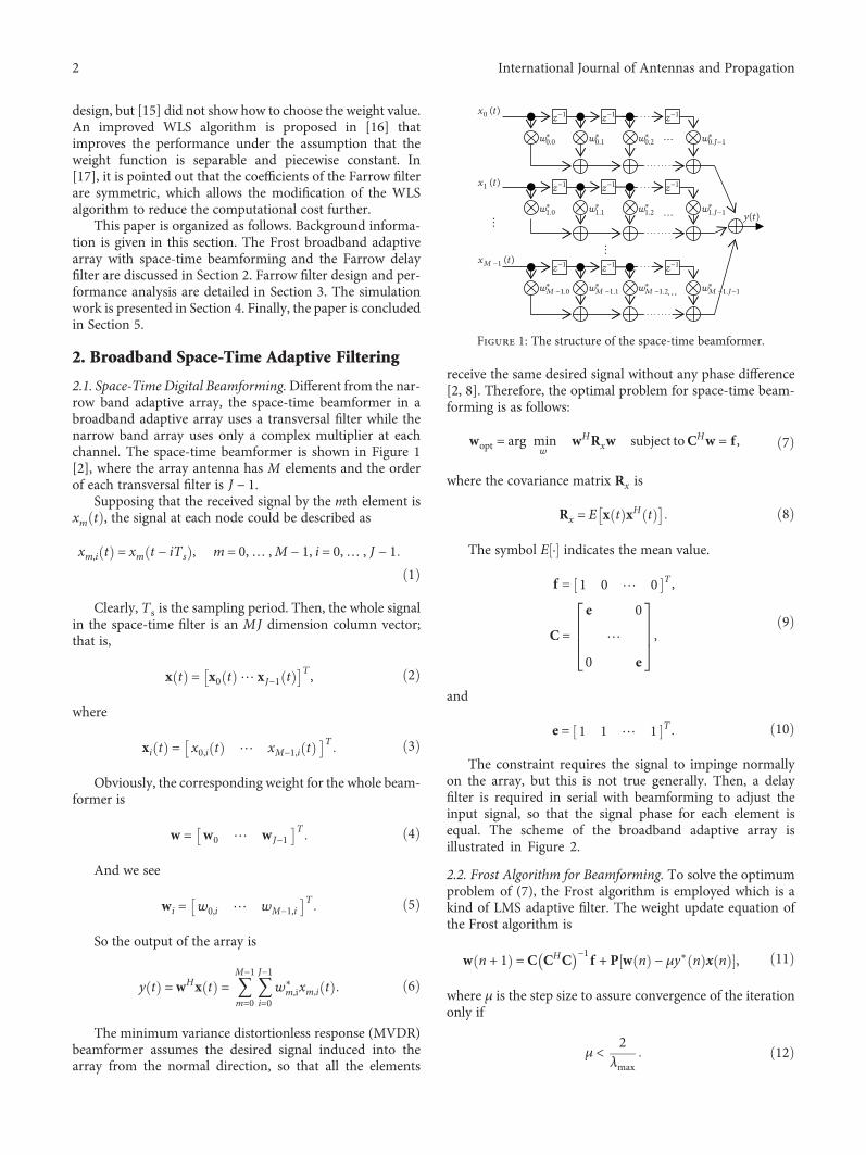
2.1. Space-Time Digital Beamforming.Different from the nar-row band adaptive array, the space-time beamformer in abroadband adaptive array uses a transversal filter while thenarrow band array uses only a complex multiplier at eachchannel. The space-time beamformer is shown in Figure 1[2], where the array antenna has M elements and the orderof each transversal filter is J − 1.

Supposing that the received signal by the mth element isxm t , the signal at each node could be described as

xm,i t = xm t − iTs , m = 0,… ,M − 1, i = 0,… , J − 11

Clearly, Ts is the sampling period. Then, the whole signalin the space-time filter is an MJ dimension column vector;that is,

x t = x0 t ⋯ x J−1 t T , 2

where

xi t = x0,i t ⋯ xM−1,i tT 3

Obviously, the corresponding weight for the whole beam-former is

w = w0 ⋯ w J−1T 4

And we see

wi = w0,i ⋯ wM−1,iT 5

So the output of the array is

y t =wHx t = 〠M−1

m=0〠J−1

i=0w∗

m,ixm,i t 6

The minimum variance distortionless response (MVDR)beamformer assumes the desired signal induced into thearray from the normal direction, so that all the elements

receive the same desired signal without any phase difference[2, 8]. Therefore, the optimal problem for space-time beam-forming is as follows:

wopt = arg minw

 wHRxw subject toCHw = f , 7

where the covariance matrix Rx is

Rx = E x t xH t 8

The symbol E · indicates the mean value.

f = 1 0 ⋯ 0 T ,

C =e 0

⋯

0 e,

9

and

e = 1 1 ⋯ 1 T 10

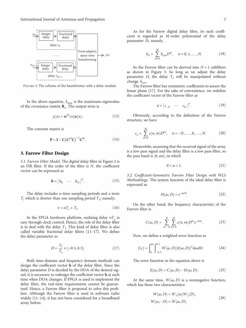
The constraint requires the signal to impinge normallyon the array, but this is not true generally. Then, a delayfilter is required in serial with beamforming to adjust theinput signal, so that the signal phase for each element isequal. The scheme of the broadband adaptive array isillustrated in Figure 2.

2.2. Frost Algorithm for Beamforming. To solve the optimumproblem of (7), the Frost algorithm is employed which is akind of LMS adaptive filter. The weight update equation ofthe Frost algorithm is

w n + 1 =C CHC −1 f + P w n − μy∗ n x n , 11

where μ is the step size to assure convergence of the iterationonly if

μ < 2λmax

12

w⁎0.0 w

⁎0.1 w

⁎0.2

w⁎1.0 w

⁎1.1 w

⁎1.2

w⁎0.J−1

w⁎1.J−1

x0 (t)

y(t)

x1 (t)

xM −1 (t)

z−1 z−1 z−1

z−1 z−1 z−1

z−1 z−1 z−1

…

…

…

…

w⁎M −1.0 w

⁎M −1.1 w

⁎M −1.2 w

⁎M −1.J−1…

Figure 1: The structure of the space-time beamformer.

2 International Journal of Antennas and Propagation

In the above equation, λmax is the maximum eigenvalueof the covariance matrix Rx. The output term is

y n =wH n x n 13

The constant matrix is

P = I −C CHC −1CH 14

3. Farrow Filter Design

3.1. Farrow Filter Model. The digital delay filter in Figure 2 isan FIR filter. If the order of the filter is N , the coefficientvector can be expressed as

h = h0 ⋯ hNT 15

The delay includes n-time sampling periods and a termTl which is shorter than one sampling period Ts; namely,

τ = nTs + Tl 16

In the FPGA hardware platform, realizing delay nTs iseasy through clock control. Hence, the role of the delay filteris to deal with the delay Tl. This kind of delay filter is alsocalled variable fractional delay filters [11–17]. We definethe delay parameter as

D = Tl

Ts∈ −0 5, 0 5 17

Both time-domain and frequency-domain methods candesign the coefficient vector h of the delay filter. Since thedelay parameter D is decided by the DOA of the desired sig-nal, it is necessary to redesign the coefficient vector h at eachtime when DOA changes. If FPGA is used to implement thedelay filter, the real-time requirements cannot be guaran-teed. Hence, a Farrow filter is proposed to solve this prob-lem. Although the Farrow filter is used in software radiowidely [11–14], it has not been considered for a broadbandarray before.

As for the Farrow digital delay filter, its each coeffi-cient is regarded as M-order polynomial of the delayparameter D; namely,

hn = 〠M

m=0hnmD

m, n = 0, 1,… ,N 18

So the Farrow filter can be derived into N + 1 subfiltersas shown in Figure 3. So long as we adjust the delayparameter D, the delay Tl will be manipulated withoutchange hnm.

The Farrow filter has symmetric coefficients to assure thelinear phase [17]. For the sake of convenience, we redefinethe coefficient vector of the Farrow filter as

c = c−N ⋯ cNT 19

Obviously, according to the definition of the Farrowstructure, we have

cn = 〠M

m=0c n,m Dm, n = −N ,… , 0,… ,N 20

Meanwhile, assuming that the received signal of the arrayis a low pass signal and the delay filter is a low pass filter, sothe pass band is 0, απ , in which

0 < α < 1 21

3.2. Coefficient-Symmetric Farrow Filter Design with WLSMethodology. The system function of the ideal delay filter isexpressed as

H ω,D = e−jωD 22

On the other hand, the frequency characteristic of theFarrow filter is

C ω,D = 〠N

n=−N〠M

m=0c n,m Dme−jnω 23

Now, we define a weighted error function as

J c =απ

0

0 5

−0 5W ω,D E ω,D 2dωdD 24

The error function in the equation above is

E ω,D = C ω,D −H ω,D 25

At the same time, W ω,D is a nonnegative function,which has these two characteristics:

W ω,D =W1 ω W2 D ,W ω, −D =W ω,D

26

……

Integerdelay

Frost adaptivespace‐time

beamforming

x0

xM−1

y(t)

Fractionaldelay

Integerdelay

Fractionaldelay

delay 𝜏0

delay 𝜏M−1

Figure 2: The scheme of the beamformer with a delay module.

3International Journal of Antennas and Propagation

With regard to the definitions above, Farrow filter designis a process of looking for suitable coefficient set c, namely,c n,m , to minimize J c according to the band width απand delay parameter D.

Since the coefficients of the Farrow Filter are symmetric,we have the conclusion that

c −n,m =c n,m ,  evenm,−c n,m ,  oddm,

c 0,m = 0, oddm27

By substituting the conclusion into (23), we get

C ω,D = aTBepe − jbTBopo, 28

where

a = 1 cos ω ⋯ cos Nω T , 29

b = 1 sin ω ⋯ sin Nω T , 30

Be =

β 0, 0 β 0, 2 β 0, 4 ⋯ β 0,M − 1β 1, 0 β 1, 2 β 1, 4 ⋯ β 1,M − 1⋮ ⋮ ⋮ ⋮ ⋮

β N , 0 β N , 2 β N , 4 ⋯ β N ,M − 1

,

31

Bo =

β 1, 1 β 1, 3 β 1, 5 … β 1,Mβ 2, 1 β 2, 3 β 2, 5 … β 2,M⋮ ⋮ ⋮ ⋮ ⋮

β N , 1 β N , 3 β N , 5 … β N ,M32

The element of the matrix is

β 0, 2m′ = c 0, 2m′ , n = 0,

β n, 2m′ = 2c n, 2m′ , n > 0,

β n, 2m′ + 1 = 2c n, 2m′ + 1 , n > 0,

m′ = 0,… ,M′

33

Substituting the result above into error function and tak-ing the conjugate property of the weighted function into con-sideration, we get the weighted error function.

J c = J Be, Bo =απ

0

0 5

0W ω,D E ω,D 2dωdD

34

Compared to (24), the integration of the delay param-eter D is defined in 0, 0 5 . Hence, the process to solve cn,m can be converted into the process to solve thematrix Be, Bo which minimizes J Be, Bo .

The weighted error function can be expressed as

J Be, Bo = −2tr Be,A1 + tr BeA2BTe A3 + tr BoA4BT

oA5

− 2tr BoA6 + constant,35

in which

A1 =απ

0

0 5

0W1 ω W2 D cos ωD peaTdωdD,

A2 =0 5

0W2 D pepTe dD,

A3 =απ

0W1 ω aaTdω,

A4 =0 5

0W2 D popTo dD,

A5 =απ

0W1 ω bbTdω,

A6 =απ

0

0 5

0W1 ω W2 D sin ωD pobTdωdD,

36

while

pe = D0 D2 ⋯ DM−1 T ,

po = D1 D3 ⋯ DM T37

Assuming that the weight is known, all the equationsabove can be solved. Considering that A2, A3, A4, and A5are symmetric and positively definite, they can be factorized

…

…

…

…hN−1

hN1

hN0

hNMhN

h0

D

z−1

z−1

x(n)

Figure 3: The structure of the Farrow filter.

4 International Journal of Antennas and Propagation

into U2, U3, U4, and U5, respectively, via the Choleskyfactorization.

Finally, according to the Lagrangian multiplier method,taking the derivative of J Be, Bo and letting it to be zero,we get

Be =U−13 UT

3AT1U−1

2 U−T2 ,

Bo =U−15 UT

5AT6U−1

4 U−T4

38

According to the definition (31), (32), and (33), c n,mcan be determined.

3.3. Weight Determination. Generally, the weightW ω,D isunknown to us. In order to decide the correct W ω,D ,iterative design is proposed. When beginning to design,we often let

W1 ω =W2 D = 1 39

Following the methodology in the previous section, wecan obtain the designed coefficient c n,m . Then, wedefine the relative error as

εe =απ0

0 5−0 5 E ω,D 2dωdD

απ0

0 5−0 5 H ω,D 2dωdD

1/2

× 100% 40

If the required relative error cannot be satisfied, wedefine the weight function as segmentation:

W1 ω =s1, ω ∈ 0, ω0 ,s2, ω ∈ ω0, αω ,

W2 D =s3, D ∈ 0,D0 ,s4, D ∈ D0, 0 5

41

For some interval with greater error, we set a largerweight and redesign C ω,D . Then, the error in this inter-val could be reduced.

4. Simulation Result

4.1. Proposed WLS Farrow Filter Design Methodology. In oursimulations, we use a linear array with 5 elements. The radiofrequency and intermediate frequency of the received signalare 2GHz and 400MHz, respectively. Assuming that thesampling frequency is 1.25GHz and the bandwidth is300MHz, the signal frequency is located in the interval[0,0 9π] since the first Nyquist domain is 0~312MHz. Inaddition, the delay interval is [0,0 5]. We set the order ofthe Farrow delay filter as N = 34 and M = 7.

We prove the validity of the proposed methodology forthe Farrow filter design by evaluating the error E ω,D , asdefined in (25). We set the initial weight function as in (39)and compute the coefficient of the Farrow filter by the stepslisted in Section 3.2. After obtaining the coefficient vector c,it is easy to get the amplitude error E ω,D as shown inFigure 4.

We focus on the interval where the desired signal exits.We notice that the large error is located in the intervals[0,0 88π] and [0 4,0 5]. If this error meets the requirement,we finish the design and take c as the final result. And ifnot, we enlarge the weight function such as

W1 ω =9700,  ω ∈ 0, 0 88π ,1,  ω ∈ 0 88π, 0 9π ,

W2 D =1,  D ∈ 0, 0 4 ,3700,  D ∈ 0 4, 0 5 ,

42

and we redesign the Farrow filter again. The new error isshown in Figure 5, where the error is less than about 6 dB(Figure 4) due to the weight function. In fact, the error is alsoimpacted by the order of the Farrow filter which will be dis-cussed in the next section.

4.2. Influence of the Filter Order. At the same simulation con-dition as the above, we only change the order of the filter andcompare the error between the proposed Farrow and directform structure in [6–8]. A comparison of the relative errorεe, defined in (40), for different filter structures is listed inTable 1. The result in Table 1 illustrates that the direct form

0

−50

−100

−150

−200

−250

0

−50

−100

−150

−200

X: 0.5Y: 2.76Z: −101.4

−250

−0.5

0.5

0

01

2

Frequency paramenter 𝜔 (0~pi)Delay parameter D (s)

Am

plitu

de er

ror 𝜀

(dB)

3

Figure 4: Error with weight function by (39).

0

−50

−100

−150

−200

−250−0.5

Am

plitu

de er

ror 𝜀

(dB)

0.5

0

Delay parameter D (s) 01

2

Frequency paramenter 𝜔 (0~pi)

3

0

−20

−80

−120

−160

−200

−180

−140

−100

−60

−40

X: 0.5Y: 2.76Z: −117.4

Figure 5: Error with weight function by (42).

5International Journal of Antennas and Propagation

structure filter outperforms the Farrow filter if the order issmall. However, when the order of the filter is large, the Far-row structure outperforms the direct form filters. Note thatthe filter with the direct form structure has to be redesignedonline when the time delay D changes. And hence it is notsuitable for the condition where the DOA changes fast. Onthe other hand, the Farrow filter needs to be designed in anoff-line manner only once and adjusts the input D to changethe delay time as shown in Figure 3.

Figure 6 illustrates the relative error with differentM andN . It shows that as the order of the Farrow filter increases, therelative error εe decreases rapidly. But once the order is largeenough, the performance keeps constant.

4.3. Computational Complexity. The WLS algorithm todesign the Farrow filter in [17] does not consider symmetriccoefficient property. Under the same conditions, we comparethe computational complexity between the proposed meth-odology and the one in [17]. The order of the Farrowdelay filter is set with N = 34 and M = 7. The running timeof the MATLAB program and the error are listed inTable 2, where the CPU frequency is 2.4GHz. We cansee that the new approach could reduce the computationalcomplexity about 50% with the similar relative error ascompared to the reference methodology.

4.4. Beamforming Based on the Farrow Filter. To investigatethe function of the Farrow filter in a space-time two-dimensional filter, we do the simulation about the array pat-tern. Suppose that the desired signal induces on the arraywith θ0 = 25° and the DOA of one strong interference isθ1 = 60

°. The radio frequencies of the two signals are both2GHz and the bandwidths are both 400MHz.

Without a Farrow filter, the pattern is shown in Figure 7by a dashed red line, where there are two nulls at θ0 = 25°andθ1 = 60°, respectively. That means that the desired signal andinterference are both suppressed. The other three lines inFigure 7 are the pattern when the delay filter is used throughthe three methodologies such as time domain [6, 8], fre-quency domain [7], and Farrow. They are very similarbecause the delay filters play the same functions. The

Table 1: Relative error with different filter orders.

Design methodOrder

4 6 12 30 56εe εe εe εe εe

Time domain [6, 8] 7.92% 7.01% 5.43% 3.70% 2.82%

Frequency domain [7] 6.80% 5.17% 2.82% 0.76% 0.17%

Farrow structure 15.23% 13.25% 3.55% 1.54% 0.74%

Rela

tive e

rror

𝜀 e

0.2

0.14

01

0.06

0.02

Order NOrder M

010

20 0 5 10 15 20

0

0.05

0.1

0.15

0.2

0.25

0.04

0.08

0.12

0.160.18

Figure 6: Error of the proposed Farrow filter with the order MN .

Table 2: Comparison of computational complexity.

Clock (s) εe (%)

Approach in [17] 4.605646 1 132E − 04New approach 2.331195 1 128E − 04

0

−10

−20

−30

−40

Patte

rn (d

B)

−50

−60

−70

−800 5 10 15 20 25 30 35 40 45

𝜃 (degree)50 55 60 65 70 75 80 85 90

Time domainFrequency domain

FarrowWithout a delay filter

Figure 7: Patterns for broadband beamforming.

−35

−40

−45

−50

Patte

rn (d

B)

𝜃 (degree)59 60 61 62 53

−55

−60

−65

−70

Time domainFrequency domain

FarrowWithout a delay filter

Figure 8: The nulls in the pattern for interference.

6 International Journal of Antennas and Propagation

interference is mitigated since the null still appears at θ = 60°.The main lobe points to θ = 0° where the desired signal isimpinging due to the role of calibration by the delay filter.Clearly, the result means that the delay filter could keep thedesired signal to satisfy the requirement of the Frost algo-rithm. And it also proves that our proposed methodologyfor Farrow filter design is right.

If we zoom in the null in Figure 8, it can be seen that thedepth is different. This is because the error of the delay filteris different. With the same filter order 56, the result is consis-tent with the result shown in Table 1 and that less errormeans deeper null.

5. Conclusion

The Farrow delay filter is taken in the broadband adaptivearray instead of the delay filter with a direct form structure.A new methodology is presented to design the Farrow filteraccording to the symmetric coefficient. The computationalcost is lower than that of the classic WLS algorithm.Although the Farrow filter is suited to the FPGA platform,the coefficient computation is heavily complicated. How tochoose the order of the Farrow filter and error requirementis an important work in the future.

Data Availability

The data used to support the findings of this study are avail-able from the corresponding author upon request.

Conflicts of Interest

The authors declare that they have no financial and personalrelationships with other people or organizations that caninappropriately influence their work; there are no profes-sional or other personal interests of any nature or kind inany product, service, and company that could be construedas influencing the position presented in the paper.

Acknowledgments

The authors would like to acknowledge the support of inno-vation funds from China Academy of Space Technology(Project no. CAST2016021) and funds from ChongqingUniversity (Project no. 2018CDGFTX0014).

References

[1] W. F. Gabriel, “Adaptive processing array systems,” Proceed-ings of the IEEE, vol. 80, no. 1, pp. 152–162, 1992.

[2] W. Liu and S. Weiss, Wideband Beamforming - Concepts andTechniques, John Wiley & Sons, Ltd, 2010.

[3] M. S. Hossain, G. N. Milford, M. C. Reed, and L. C. Godara,“Efficient robust broadband antenna array processor in thepresence of look direction errors,” IEEE Transactions onAntennas and Propagation, vol. 61, no. 2, pp. 718–727, 2013.

[4] W. Liu, R. Wu, and R. J. Langley, “Design and analysis ofbroadband beamspace adaptive arrays,” IEEE Transactionson Antennas and Propagation, vol. 55, no. 12, pp. 3413–3420,2007.

[5] T. K. Sarkar, H. Wang, S. Park et al., “A deterministic least-squares approach to space–time adaptive processing (STAP),”IEEE Transactions on Antennas and Propagation, vol. 49,no. 1, pp. 91–103, 2001.

[6] T. I. Laakso, V. Valimaki, M. Karjalainen, and U. K. Laine,“Splitting the unit delay [FIR/all pass filters design],” IEEE Sig-nal Processing Magazine, vol. 13, no. 1, pp. 30–60, 1996.

[7] G. Oetken, T. Parks, and H. Schussler, “New results in thedesign of digital interpolators,” IEEETransactions onAcoustics,Speech, and Signal Processing, vol. 23, no. 3, pp. 301–309, 1975.

[8] Z. Ahmad, S. Yaoliang, and Q. du, “Adaptive wideband beam-forming based on digital delay filter,” Journal of Microwaves,Optoelectronics and Electromagnetic Applications, vol. 15,no. 3, pp. 261–274, 2016.

[9] H. Li, G. Torfs, T. Kazaz, J. Bauwelinck, and P. Demeester,“Farrow structured variable fractional delay Lagrange filterswith improved midpoint response,” in 2017 40th InternationalConference on Telecommunications and Signal Processing(TSP), pp. 506–509, Barcelona, Spain, 2017.

[10] C. W. Farrow, “A continuously variable digital delay element,”in 1988 IEEE International Symposium on Circuits and Sys-tems, vol. 3, pp. 2641–2645, Espoo, Finla, 1988.

[11] H. Johansson, “Farrow-structure-based reconfigurable band-pass linear-phase FIR filters for integer sampling rate conver-sion,” IEEE Transactions on Circuits and Systems II: ExpressBriefs, vol. 58, no. 1, pp. 46–50, 2011.

[12] M. Abbas, O. Gustafsson, and H. Johansson, “On the fixed-point implementation of fractional-delay filters based on thefarrow structure,” IEEE Transactions on Circuits and SystemsI: Regular Papers, vol. 60, no. 4, pp. 926–937, 2013.

[13] J. Vesma and T. Saramaki, “Design and properties ofpolynomial-based fractional delay filters,” in 2000 IEEEInternational Symposium on Circuits and Systems, vol. 1,pp. 104–107, Geneva, Switzerland, 2000.

[14] T. Ma, Y. Wei, and X. J. Ma, “A newmethod for designing Far-row filters based on cosine basis neural network,” in 2017 IEEEInternational Conference on Digital Signal Processing, pp. 154–158, Beijing, China, 2017.

[15] A. Tarczynski, G. D. Cain, E. Hermanowicz, and M. Rojewski,“WLS design of variable frequency response FIR filters,” in1997 IEEE International Symposium on Circuits and Systems,vol. 4, pp. 2244–2247, Hong Kong, 1997.

[16] W.-S. Lu and T.-B. Deng, “An improved weighted least-squares design for variable fractional delay FIR filters,” IEEETransactions on Circuits and Systems II: Analog and DigitalSignal Processing, vol. 46, no. 8, pp. 1035–1040, 1999.

[17] T. B. Deng, “Symmetry-based low-complexity variablefractional-delay FIR filters,” in 2004 IEEE InternationalSymposium on Communications and Information Technology,vol. 1, pp. 194–199, Sapporo, Japan, 2004.

7International Journal of Antennas and Propagation

International Journal of

AerospaceEngineeringHindawiwww.hindawi.com Volume 2018

RoboticsJournal of

Hindawiwww.hindawi.com Volume 2018

Hindawiwww.hindawi.com Volume 2018

Active and Passive Electronic Components

VLSI Design

Hindawiwww.hindawi.com Volume 2018

Hindawiwww.hindawi.com Volume 2018

Shock and Vibration

Hindawiwww.hindawi.com Volume 2018

Civil EngineeringAdvances in

Acoustics and VibrationAdvances in

Hindawiwww.hindawi.com Volume 2018

Hindawiwww.hindawi.com Volume 2018

Electrical and Computer Engineering

Journal of

Advances inOptoElectronics

Hindawiwww.hindawi.com

Volume 2018

Hindawi Publishing Corporation http://www.hindawi.com Volume 2013Hindawiwww.hindawi.com

The Scientific World Journal

Volume 2018

Control Scienceand Engineering

Journal of

Hindawiwww.hindawi.com Volume 2018

Hindawiwww.hindawi.com

Journal ofEngineeringVolume 2018

SensorsJournal of

Hindawiwww.hindawi.com Volume 2018

International Journal of

RotatingMachinery

Hindawiwww.hindawi.com Volume 2018

Modelling &Simulationin EngineeringHindawiwww.hindawi.com Volume 2018

Hindawiwww.hindawi.com Volume 2018

Chemical EngineeringInternational Journal of Antennas and

Propagation

International Journal of

Hindawiwww.hindawi.com Volume 2018

Hindawiwww.hindawi.com Volume 2018

Navigation and Observation

International Journal of

Hindawi

www.hindawi.com Volume 2018

Advances in

Multimedia

Submit your manuscripts atwww.hindawi.com