Bristol Bay Data Summary Report 2012 - NOAA in Alaska · Bristol Bay Data Summary Report May 2012...
65
Coastal Habitat Mapping Program Bristol Bay Data Summary Report May 2012 Prepared for: NOAA National Marine Fisheries Service Alaska Region
Transcript of Bristol Bay Data Summary Report 2012 - NOAA in Alaska · Bristol Bay Data Summary Report May 2012...
Coastal Habitat Mapping Program
Bristol BayData Summary Report
May 2012
Prepared for:NOAA National Marine
Fisheries ServiceAlaska Region

On the Cover: Strogonof Point North of Port Heiden Port Moller Cinder River

CORI Project: 11-23 May 2012
ShoreZone Coastal Habitat Mapping Data Summary Report
2006 Survey Area, Bristol Bay
Prepared for: NOAA National Marine Fisheries Service, Alaska Region
Prepared by:
COASTAL & OCEAN RESOURCES INC 759A Vanalman Ave., Victoria BC V8Z 3B8 Canada
(250) 658-4050 www.coastalandoceans.com
ARCHIPELAGO MARINE RESEARCH LTD 525 Head Street, Victoria BC V9A 5S1 Canada
(250) 383-4535 www.archipelago.ca

May 2012 Bristol Bay Alaska Summary (NOAA) 2

May 2012 Bristol Bay Alaska Summary (NOAA) 3
SUMMARY
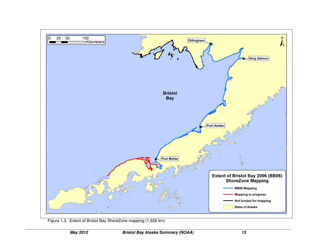
ShoreZone is a coastal habitat mapping and classification system in which georeferenced aerial imagery is collected specifically for the interpretation and integration of geological and biological features of the intertidal zone and nearshore environment. The mapping methodology is summarized in Harney et al (2008). This interim data summary report provides information on geomorphic and biological features of 1,626 km of shoreline mapped for the 2006 survey of Bristol Bay, Alaska. The habitat inventory is comprised of 912 along-shore segments (units), averaging 1,783 m in length (note that the AK Coast 1:63,360 digital shoreline shows this mapping area encompassing 1,262 km, but mapping data based on better digital shorelines represent the same area with 1,626km stretching along the coast). Organic shorelines (such as estuaries) are mapped along 541 km (33%) of the study area. Bedrock shorelines (BC Classes 1-5) are virtually non-existent along the shoreline with only (0.02%) mapped. A little more than half (55%) of the mapped coastal environment is characterized as sediment-dominated shorelines (BC Classes 21-30). Of these, wide sand and gravel flats (BC Class 24) are the most common, mapped along 370 km of shoreline (23% of the total study area). Approximately 70% of all habitat classes mapped are structured by wave energy and another 29% is structured by estuarine processes; fluvial processes are the dominant structuring force in this habitat class. Repeatable assemblages of biota that can be recognized from the aerial imagery are termed biobands; 8 biobands have been mapped in Bristol Bay to date. Fox example, Dune Grass occurs along 88% of the shoreline mapped, a surprisingly high percentage of the coast. Man-modified shorelines are comparatively rare (<1%). The most common types of shore modification observed are riprap and wooden bulkheads (3.6 km each), followed by landfill (2.4 km) and boat ramps (1.1 km). Most anthropogenic features occur in the communities of King Salmon and Egegik Bay. Mapping data can be accessed via the Alaska ShoreZone Mapping Website at: www.shorezone.org

May 2012 Bristol Bay Alaska Summary (NOAA) 4

May 2012 Bristol Bay Alaska Summary (NOAA) 5
TABLE OF CONTENTS
SECTION TITLE PREFACE Summary 3 Table of Contents 5 List of Tables 6 List of Figures 7 1 INTRODUCTION 9 1.1 Overview of the ShoreZone Coastal Habitat Mapping Program 9 1.2 ShoreZone Mapping of Bristol Bay 10 2 PHYSICAL SHOREZONE DATA SUMMARY 15 2.1 Shore Types 15 2.2 Anthropogenic Shore Modifications 22 2.3 Oil Residence Index (ORI) 22 2.4 Wave Exposure 26 3 BIOLOGICAL SHOREZONE DATA SUMMARY 29 3.1 Biobands 29 3.2 Habitat Class 36 4 REFERENCES 40 5 ACKNOWLEDGMENTS 41 APPENDIX A: DATA DICTIONARY

May 2012 Bristol Bay Alaska Summary (NOAA) 6
LIST OF TABLES
Table
Description Page
2.1 Summary of Shore Types 16 2.2 Summary of Shore Types by ESI 20 2.3 Summary of Shore Modifications 22 2.4 Summary of Oil Residence Index 24 2.5 Summary of Wave Exposure 27 3.1 Bioband Abundances Mapped 31 3.2 Summary of Habitat Classes 38

May 2012 Bristol Bay Alaska Summary (NOAA) 7
LIST OF FIGURES
Figure
Description Page
1.1 Extent of ShoreZone imagery in Alaska, BC, and Washington. 11 1.2 Extent of ShoreZone imagery mapping in Alaska. 12 1.3 Extent of ShoreZone mapping in Bristol Bay 2006. 13 1.4 Map of study area in Bristol Bay 2006. 14 2.1 Map of the distribution of principal substrate types. 17 2.2 Relative abundance of principal substrate types. 18 2.3 Relative abundance of sediment shorelines. 18 2.4 Map of the distribution of sediment shorelines. 19 2.5 Distribution of beaches and tidal flats on the basis of grouped
ESI class. 21
2.6 Map of the distribution of units with shore modifications. 23 2.7 Oil Residence Index (ORI) for shorelines in Bristol Bay. 25 2.8 Summary of wave exposure in Bristol Bay. 27 2.9 Distribution of wave exposure categories. 28 3.1 Example of biobands. 29 3.2 Bioband abundances. 31 3.3 Distribution of Dune Grass, Salt Marsh and Sedges Biobands. 33 3.4 Distribution of bioareas. 35 3.5 Summary of habitat occurrence. 37 3.6 Distribution of Estuary Habitat Class in Bristol Bay. 39

May 2012 Bristol Bay Alaska Summary (NOAA) 8

May 2012 Bristol Bay Alaska Summary (NOAA) 9
1 INTRODUCTION
1.1 Overview of the ShoreZone Coastal Habitat Mapping Program The land-sea interface is a crucial realm for terrestrial and marine organisms, human activities, and dynamic processes. ShoreZone is a mapping and classification system that specializes in the collection and interpretation of aerial imagery of the coastal environment. Its objective is to produce an integrated, searchable inventory of geomorphic and biological features of the intertidal and nearshore zones which can be used as a tool for science, education, management, and environmental hazard planning. ShoreZone imagery provides a useful baseline, while mapped resources (such as shoreline sediments, eelgrass and wetland distributions) are an important tool for scientists and managers. The ShoreZone system was employed in the 1980s and 1990s to map coastal features in British Columbia and Washington State (Howes 2001; Berry et al 2004). Between 2001 and 2003, ShoreZone imaging and mapping was initiated in the Gulf of Alaska, beginning with Cook Inlet, Outer Kenai, Katmai, and portions of the Kodiak Archipelago (Harper and Morris 2004). The ShoreZone program in Alaska continues to grow through the efforts of a network of partners, including scientists, managers, GIS specialists, and web specialists in federal, state, and local government agencies and in private and nonprofit organizations. The coastal mapping data and imagery are used for oil spill contingency planning, conservation planning, habitat research, development evaluation, mariculture site review, and recreation opportunities. Protocols and standards are updated through technological advancements (e.g. Harney et al 2008), and applications are developed that use ShoreZone data to examine modern questions regarding the coastal environment and nearshore habitats (Harney 2007, 2008). As of May 2012, mapped regions include close to 46,500 km of coastline in the Gulf of Alaska and 40,000 km of coastline in British Columbia and Washington State (Figures 1.1, 1.2 and 1.3). The ShoreZone mapping system provides a spatial framework for coastal habitat assessment on local and regional scales. Research and practical applications of ShoreZone data and imagery include:
• natural resource and conservation planning • environmental hazard response • spill contingency planning • linking habitat use and life-history strategy of nearshore fish and other
intertidal organisms • habitat suitability modeling (for example, to predict the spread of invasive
species or the distribution of beaches appropriate for spawning fish • development evaluation and mariculture site review

May 2012 Bristol Bay Alaska Summary (NOAA) 10
• ground-truthing of aerial data on smaller spatial scales • public use for recreation, education, outreach, and conservation
Details concerning mapping methodology and the definition of 2008 standards are available in the ShoreZone Coastal Habitat Mapping Protocol for the Gulf of Alaska (Harney et al 2008). This and other ShoreZone reports are available for download from the ShoreZone website at www.ShoreZone.org. 1.2 ShoreZone Mapping of Bristol Bay 2006 Imagery
The field survey in Bristol Bay conducted in 2006 collected aerial video and digital still photographs of the coastal and nearshore zone during zero-meter tide levels and lower. The imagery and associated audio commentary are used to map the geomorphic and biological features of the shoreline according to the ShoreZone Coastal Habitat Mapping Protocol (Harney et al 2008). The purpose of this report is to provide a summary of the physical (geomorphic) and biological data mapped in the study area to date (Bristol Bay; Figure 1.4). The along-shore length of shoreline mapped in the BB06 database is 1,626 kilometers in 912 along-shore segments (units), averaging 1,783 m in length. Physical and biological data are summarized with illustrations in Sections 2 and 3, respectively.

May 2012 Bristol Bay Alaska Summary (NOAA) 11
Figure 1.1. Extent of ShoreZone imagery in Alaska, British Columbia, and Washington State and Oregon (96,482 km).

May 2012 Bristol Bay Alaska Summary (NOAA) 12
Figure 1.2. Extent of ShoreZone imagery (52,123 km) and coastal habitat mapping in the State of Alaska (as of May 2012).
May 2012 Bristol Bay Alaska Summary (NOAA) 13
Figure 1.3. Extent of Bristol Bay ShoreZone mapping (1,626 km)

May 2012 Bristol Bay Alaska Summary (NOAA) 14
Figure 1.4. Map of the study area imaged in Bristol Bay in 2006; physical (geomorphic) and biological ShoreZone data are summarized in this report (1,626 km).

May 2012 Bristol Bay Alaska Summary (NOAA) 15
2 PHYSICAL SHOREZONE DATA SUMMARY
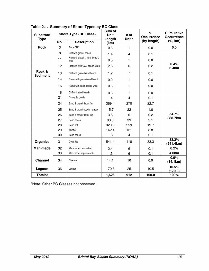
2.1 Shore Types The principal characteristics of each along-shore segment are used to assign an overall unit classification or “shore type” that represents the unit as a whole. ShoreZone mapping employs two along-shore unit classification systems: coastal shore types defined for British Columbia (“BC Class”) and the “Environmental Sensitivity Index” (ESI) class developed for oil-spill mitigation. A third shoreline classification system unique to ShoreZone (“Habitat Class”) is defined in Section 3.3. The BC Class system is used to describe along-shore coastal units as one of 36 shore types defined on the basis of the geomorphic features, substrate, sediment texture, across-shore width, and slope of that section of coastline (after Howes et al 1994; Appendix A, Table A-2). Coastal classes also characterize units dominated by organic shorelines such as marshes and estuaries (BC Class 31), man-made features (BC Classes 32 and 33), high-current channels (BC Class 34), glaciers (BC Class 35) and Lagoons (BC Class 36). The occurrence of BC shore types in the study area is listed in Table 2.1. Grouped BC Classes are useful to illustrate mapped distributions (Figure 2.1) and to summarize data in graphic form (Figure 2.2). Bedrock shorelines (BC Classes 1-5) comprise 0.3 km (<1%) of mapped shorelines. Rock and sediment shorelines (BC Classes 6-20) also comprise less than 1% of the shoreline (0.4km). Sediment-dominated shorelines (BC Classes 21-30) comprise more than half the entire area (54.7%) along 888.7km of the coastline (Figures 2.3 & 2.4). Of these, wide sand and gravel flats (BC Class 24) are the most common, mapped along 369.4km of shoreline (22.7% of the total study area). Estuaries and Lagoons constitute the remaining shoreline with 33.3% and 10.5% respectively. The NOAA Environmental Sensitivity Index (ESI Class) is a shoreline classification system developed to categorize coastal regions on the basis of their oil-spill sensitivity. The ESI system uses wave exposure and principal substrate type to assign alongshore coastal units a ranking of 1-10 to indicate the relative degree of sensitivity to oil spills (1=least sensitive, 10=most sensitive) as well as a general shore type (Peterson et al 2002; Appendix A, Table A-3). The ESI system is an integral component of oil-spill contingency planning. Substrate permeability is of principal importance in estimating the residence time of oil on the shoreline, thus sediment texture is a key element in determining the ESI class. The occurrence of ESI shore types in the study area is listed in Table 2.2. The distribution of beaches and tidal flats (on the basis of mapped ESI class referring to sediment texture) is shown in Figure 2.5.
May 2012 Bristol Bay Alaska Summary (NOAA) 16
Table 2.1. Summary of Shore Types by BC Class
Substrate Type
Shore Type (BC Class) Sum of
Unit Length
(km)
# of Units
% Occurrence (by length)
Cumulative Occurrence
(%, km) No. Description
Rock 3 Rock Cliff 0.3 1 0.0 0.0
8 Cliff with gravel beach 1.4 4 0.1
11 Ramp w gravel & sand beach, wide 0.3 1 0.0
12 Platform with G&S beach, wide 2.6 6 0.2 0.4% 6.4km
Rock & Sediment
13 Cliff with gravel/sand beach 1.2 7 0.1
14 Ramp with gravel/sand beach 0.2 1 0.0
16 Ramp with sand beach, wide 0.3 1 0.0
18 Cliff with sand beach 0.3 1 0.0
21 Gravel flat, wide 1.4 4 0.1
24 Sand & gravel flat or fan 369.4 270 22.7
25 Sand & gravel beach, narrow 15.7 22 1.0
26 Sand & gravel flat or fan 3.6 6 0.2 54.7% 888.7km
27 Sand beach 33.6 39 2.1
28 Sand flat 320.9 259 19.7
29 Mudflat 142.4 121 8.8
30 Sand beach 1.8 4 0.1
Organics 31 Organics 541.4 118 33.3 33.3%
(541.4km)
Man-made 32 Man-made, permeable 2.4 6 0.1 0.2%
33 Man-made, impermeable 1.5 6 0.1 4.0km
Channel 34 Channel 14.1 10 0.9 0.9%
(14.1km)
Lagoon 36 Lagoon 170.8 25 10.5 10.5% (170.8)
Totals: 1,626 912 100.0 100%
*Note: Other BC Classes not observed.

May 2012 Bristol Bay Alaska Summary (NOAA) 17
Figure 2.1. Map of the distribution of principal substrate types (on the basis of grouped BC Classes) in the study area. Data are listed by individual class and summarized by grouped classes in Table 2.1.

May 2012 Bristol Bay Alaska Summary (NOAA) 18
Figure 2.2. Relative abundance of principal substrate types (on the basis of grouped BC
Classes) in the study area. Data are summarized in Table 2.1.
Figure 2.3. Relative abundance of sediment shorelines (BC classes 21-30) in the study area.

May 2012 Bristol Bay Alaska Summary (NOAA) 19
Figure 2.4. Map of the distribution of sediment shorelines (BC Classes 21-30, grouped by geomorphology) in the study area.
Data are summarized in Table 2.1.

May 2012 Bristol Bay Alaska Summary (NOAA) 20
Table 2.2. Summary of Shore Types by ESI Class
Environmental Sensitivity Index (ESI) Sum of Unit Length (km)
# of Units
% Occurrence (by length) No. Description
3A Fine- to medium-grained sand beaches 82.9 97 5.1%
3B Scarps and steep slopes in sand 23.6 20 1.4%
4 Coarse-grained sand beaches 5.7 10 0.4%
5 Mixed sand and gravel beaches 170.5 201 10.5%
6B Gravel beaches (cobbles and boulders) 1.4 4 0.1%
6C Rip rap (man-made) 0.1 1 0.0%
7 Exposed tidal flats 327.2 172 20.1%
8A Sheltered scarps in bedrock, mud, or clay; sheltered rocky shores (impermeable)
1.9 5 0.1%
8B Sheltered, solid, man-made structures; sheltered rocky shores (permeable)
2.7 8 0.2%
8E Peat shorelines 10.1 4 0.6%
9A Sheltered tidal flats 390.3 260 24.0%
9B Vegetated low banks 34.2 19 2.1%
10A Salt- and brackish-water marshes 550.0 102 33.8%
10B Freshwater marshes 25.1 9 1.5%
Totals: 1,626 912 100.0 %
*Note: Other ESI Classes not observed.

May 2012 Bristol Bay Alaska Summary (NOAA) 21
Figure 2.5. Distribution of beaches and tidal flats on the basis of ESI class. Sand and gravel beaches refer to ESI classes 4 & 5. Gravel
beaches refer to ESI classes 6A & 6B. Tidal flats refer to ESI class 9A & 7 and are generally confined to relatively protected areas at the heads of inlets.

May 2012 Bristol Bay Alaska Summary (NOAA) 22
2.2 Anthropogenic Shore Modifications Shore-protection features and coastal access constructions such as seawalls, rip rap, docks, dikes, and wharves are enumerated in ShoreZone mapping data. Overall, shorelines classified as man-modified (having more than 50% of the unit altered by human activities, assigned BC Classes 32 and 33) occur along 12.0 km (0.7%) of shoreline in the study area, mostly in the communities of King Salmon and Egegik Bay. The types of shore modification features (such as boat ramps, bulkheads, and rip rap) and their relative proportions of the intertidal zone are mapped into the database in the “SHORE_MOD” fields of the UNIT table (see Table A-1 for a description of these fields). The distribution of shore modifications mapped in the study area (Table 2.3) is shown in Figure 2.6.
Table 2.3 Summary of Shore Modifications Shore
Modification
# of Occurrences
Shoreline Length (km)
% of Shoreline
Wooden bulkhead 25 3.6 30.3% Boat ramp 16 1.1 9.4% Concrete bulkhead 10 0.7 6.1% Landfill 24 2.4 19.8% Sheet pile 22 3.6 30.3% Riprap 8 0.5 4.1%
Totals: 105 12.0 100.0
2.3 Oil Residence Index (ORI) The Oil Residence Index (ORI) is a rating between 1 and 5 that reflects the estimated persistence of spilled oil on a shoreline. A value of 1 reflects relatively short oil residence (days to weeks), while a value of 5 reflects potentially long oil residence times (months to years). An ORI value is applied to each across-shore component on the basis of sediment texture and wave exposure (Table A-5), as well as to each along-shore unit on the basis of shore type and wave exposure (Table A-6). For more information on the assignment of this attribute, refer to the ShoreZone Protocol (Harney et al 2008). The dominance of lower wave exposures and sand-gravel sediment textures results in high Oil Residence Indices for most shore segments: 57% have an ORI of 4 or 5, indicating oil residence times are on the order of months to years (Table 2.4; Figure 2.7).

May 2012 Bristol Bay Alaska Summary (NOAA) 23
Figure 2.6. Map of the distribution of units in which shore modification features were observed in the
Bristol Bay study area. Data are summarized in Table 2.3.

May 2012 Bristol Bay Alaska Summary (NOAA) 24
Table 2.4. Summary of Oil Residence Index
Relative Persistence
Oil Residence
Index (ORI)
Estimated temporal
persistence
Shoreline Length
(km)
Shoreline Length
(%)
Short 1 Days to weeks 00.0 00.0% 2 Weeks to months 315.8 19.4%
Moderate 3 Weeks to months 385.5 23.7% 4 Months to years 153.9 09.5%
Long 5 Months to years 770.5 47.4% Totals: 1,626 100.0%

May 2012 Bristol Bay Alaska Summary (NOAA) 25
Figure 2.7. Oil Residence Index (ORI) for shorelines in Bristol Bay, based on substrate type and wave exposure (Appendix A, Table A-5).

May 2012 Bristol Bay Alaska Summary (NOAA) 26
2.4 Wave Exposure Wave exposure categories range from Very Protected (VP) to Very Exposed (VE) and are usually defined in ShoreZone on the basis of a typical set of biobands; but in Bristol Bay, attached intertidal and nearshore biobands are absent. The physical mappers’ estimate of wave energy (the Observed Physical Exposure attribute, based on maximum fetch measurements) was deemed to be equivalent to the biological wave exposure, and the six biological wave exposure categories are the same as those used in the physical mapping (Appendix A, Tables A-4 and A-9). The physical wave exposure is based on fetch window estimates and coastal geomorphology. The physical wave exposure, as transcribed to the biological exposure attribute for the Bristol Bay mapping, was also then used in the look up matrix for determining the Oil Residence Index (ORI) (Table A-6). The occurrence of the wave exposure categories mapped in the Bristol Bay study area is summarized in Table 2.5 and in Figure 2.8. Most of the shoreline in the study area was classified with a wave exposure of Semi-Protected (SP) or lower (66%). Twenty-three percent of the area was mapped as Exposed (E) and 10% was mapped in the Semi-Exposed (SE) category. A summary map of the wave exposure categories distribution is shown in Figure 2.9.

May 2012 Bristol Bay Alaska Summary (NOAA) 27
Table 2.5. Summary of Wave Exposure in Bristol Bay
Wave Exposure Shoreline
Length
(km)
% of
Shoreline Name Code
Exposed E 377 23%
Semi-Exposed SE 165 10%
Semi-Protected SP 332 20%
Protected P 715 45%
Very Protected VP 37 1%
Totals 1,626 100%
Figure 2.8. Summary of wave exposures mapped in the Bristol Bay.

May 2012 Bristol Bay Alaska Summary (NOAA) 28
Figure 2.9. Distribution of wave exposure categories mapped in the Bristol Bay study area.
May 2012 Bristol Bay Alaska Summary (NOAA) 29
3 BIOLOGICAL SHOREZONE DATA SUMMARY
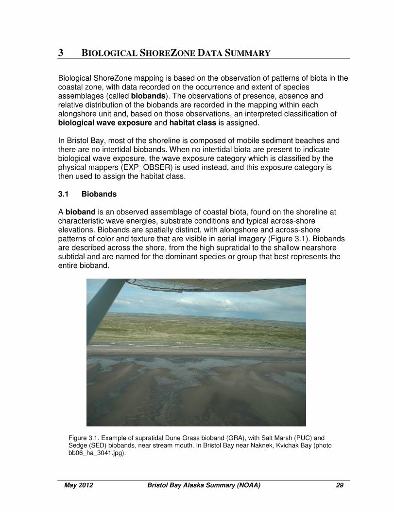
Biological ShoreZone mapping is based on the observation of patterns of biota in the coastal zone, with data recorded on the occurrence and extent of species assemblages (called biobands). The observations of presence, absence and relative distribution of the biobands are recorded in the mapping within each alongshore unit and, based on those observations, an interpreted classification of biological wave exposure and habitat class is assigned. In Bristol Bay, most of the shoreline is composed of mobile sediment beaches and there are no intertidal biobands. When no intertidal biota are present to indicate biological wave exposure, the wave exposure category which is classified by the physical mappers (EXP_OBSER) is used instead, and this exposure category is then used to assign the habitat class. 3.1 Biobands A bioband is an observed assemblage of coastal biota, found on the shoreline at characteristic wave energies, substrate conditions and typical across-shore elevations. Biobands are spatially distinct, with alongshore and across-shore patterns of color and texture that are visible in aerial imagery (Figure 3.1). Biobands are described across the shore, from the high supratidal to the shallow nearshore subtidal and are named for the dominant species or group that best represents the entire bioband.
Figure 3.1. Example of supratidal Dune Grass bioband (GRA), with Salt Marsh (PUC) and Sedge (SED) biobands, near stream mouth. In Bristol Bay near Naknek, Kvichak Bay (photo bb06_ha_3041.jpg).

May 2012 Bristol Bay Alaska Summary (NOAA) 30
Some biobands are named for a single indicator species (such as the Blue Mussel bioband (BMU)), while others represent an assemblage of co-occurring species (such as the Red Algae bioband (RED)). Indicator species are the species that are most commonly observed in the band. For descriptions of all the biobands in mapping throughout Alaska, including lists of indicator and associate species, refer to Appendix A, Table A-17. The distribution of the each bioband observed in every unit is recorded in the database. Bioband occurrence is recorded as patchy or continuous for all biobands except for the Splash Zone bioband (VER), which is recorded from an estimate of the across-shore width (narrow, medium or wide). A distribution of patchy is defined as ‘visible in less than half (approximately 25-50%) of the along-shore unit length’ and continuous is considered more than half (50-100%). Refer to Appendix A, Table A-18 for definitions for bioband occurrence. The occurrence of each bioband mapped in the Bristol Bay project area covered by this summary report is summarized in Table 3.1 and Figure 3.2. Note that the abundances for each bioband are listed by occurrences of patchy or continuous. As a result, the abundance values for the lengths and percentages of shoreline do not translate into the presence of each band along 100% of the alongshore unit length. The values under the ‘continuous’ column should be interpreted as shoreline length where the band was mapped in approximately 50-100% of the unit length, while the values under the ‘patchy’ column indicate that the bioband was visible in approximately 25-50%. Dune Grass (GRA) was the most commonly mapped bioband, with 88% of the coast having either patchy or continuous GRA recorded. Salt Marsh (PUC) bioband was the next most commonly mapped band as either patchy or continuous on 61% of the shoreline. The three supratidal biobands of Dune Grass, Sedges and Salt Marsh were by far the dominant biota observed in Bristol Bay study area. Only small amounts of biobands associated with stable substrate (Barnacle, Rockweed, Green Algae and Red Algae) were observed. Approximately 1% of shoreline was mapped with Eelgrass present. Unlike rocky coastlines on the Gulf of Alaska shores, no nearshore canopy kelps were mapped in Bristol Bay.

May 2012 Bristol Bay Alaska Summary (NOAA) 31
Table 3.1 Bioband Abundances Mapped in Bristol Bay
Bioband Continuous Patchy Total % of
Name Code (km) % (km) % (km) Mapped
Dune Grass GRA 1,183 73 249 15 1,432 88%
Sedges SED 429 26 137 8 567 35%
Salt Marsh PUC 737 45 257 16 994 61%
Barnacle BAR 5 <1 11 1 17 1%
Rockweed FUC 5 <1 9 1 14 1%
Green Algae ULV 2 <1 3 <1 5 <1%
Red Algae RED <1 <1 5 <1 5 <1%
Eelgrass ZOS 12 1 8 1 20 1%
*Note: Other Biobands not observed
Figure 3.2. Bioband abundances mapped in Bristol Bay study.
Bioband Abundances
0 10 20 30 40 50 60 70 80 90 100
ZOS
RED
ULV
FUC
BAR
PUC
SED
GRA
Bio
band C
ode
% Mapped Shoreline
Continuous Patchy

May 2012 Bristol Bay Alaska Summary (NOAA) 32
Bioband Distributions Combinations of the various biobands act as indicators for the different biological wave exposures and habitat classes. The distributions of the few most common supratidal bioband combinations are shown in Figure 3.3. Dune Grass, Sedges and Salt Marsh Biobands The three biobands that can occur in the supratidal (A zone) used to indicate salt marsh and estuarine conditions are the Dune Grass (GRA), Sedges (SED) and Salt Marsh (PUC) biobands. Each of these three biobands are dominated by rooted vascular plants, with the Salt Marsh bioband having the most diversity in species composition, including a number of salt-tolerant grasses, herbs and sedges. Further descriptions of the characteristics of these biobands can be found in Appendix A, Table A-17. Co-occurrence of these three bands, together with the presence of a freshwater stream (year-round flow) and a ‘delta’ form at the stream mouth are used to indicate an Estuary habitat class category. Usually, shorelines where all three biobands co-occur are the areas with the largest estuary salt marsh complexes, which are often found at river deltas and at the heads of inlets. Smaller estuarine features are often indicated when the Dune Grass (GRA) and the Salt Marsh (PUC) bands co-occur. The Dune Grass bioband is often observed growing on its own, in dry beach berms or among driftwood log lines, and occurs at all wave exposures, from high energy bare beaches, to sheltered salt meadows. The following combinations have been mapped below (Figure 3.3):
• Dune Grass (GRA) alone: showing where fringing grass is present (not necessarily associated with wetlands).
• Dune Grass (GRA) and Salt Marsh (PUC) occurring together: often showing locations of smaller areas of estuarine conditions.
• All three bands occurring together, Dune Grass (GRA), Salt Marsh (PUC) and Sedges (SED): showing larger estuarine areas, including stream and river mouths.
Nearly all of the Bristol Bay shoreline in this study area was mapped with at least one of these three biobands present.

May 2012 Bristol Bay Alaska Summary (NOAA) 33
Figure 3.3. Distribution of units in which select combinations of the Dune Grass, Salt Marsh and Sedges biobands were
observed in the Bristol Bay study area.

May 2012 Bristol Bay Alaska Summary (NOAA) 34
BioAreas As ShoreZone biological mapping has been completed throughout Alaska, differences in the species assemblages that characterize the coastal habitats have been observed on a broad geographic scale. Differences in biota are the most obvious in the lower intertidal and nearshore subtidal biobands. To recognize region-specific species assemblages, as well as to identify broad-scale trends in coastal habitats, a number of bioareas have been defined in Alaska (Figure 3.4 and Appendix A, Table A-8). A similar approach was applied in British Columbia to recognize the broad-scale eco-regional differences and seven bioareas have been defined there for the ShoreZone mapping. Bioareas are delineated on the basis of observed differences in the distribution of lower intertidal biota, nearshore canopy kelps, and coastal habitat classification. For example, the outer coast Southeast Alaska – Sitka bioarea has a full range of wave exposures, dense nearshore canopy kelps and a diverse array of coastal morphologies. The Bristol Bay bioarea is characterized by broad mobile bare sediment beaches, numerous broad estuary flats, and near continuous biobands of Dune Grass (GRA) and Salt Marsh (PUC) in the supratidal.

May 2012 Bristol Bay Alaska Summary (NOAA) 35
Figure 3.4. Bioareas identified in coastal Alaska ShoreZone mapping to date. Bioareas are delineated on the basis of
observed regional differences in the distribution of biota and coastal geomorphology.

May 2012 Bristol Bay Alaska Summary (NOAA) 36
3.2 Habitat Class Habitat Class is a summary classification that combines both physical and biological characteristics observed for a particular shoreline unit. The classification is based on biological wave exposure and geomorphic characteristics. The habitat class category is intended to provide a single attribute to summarize the biophysical features of the unit, based on an overall classification made from the detailed attributes that have been mapped. In the Bristol Bay study area, the habitat class is determined from the biological wave exposure as inferred from the physical wave exposure category, in combination with the ‘dominant structuring process’ and geomorphic features of the site. Wave energy is the most common structuring process, and less commonly observed habitats are those structured by current, estuarine/fluvial processes or anthropogenic structures. In wave energy-structured habitat classes, the combination of wave exposure and substrate type determines the degree of substrate mobility, which in turn determines the presence and abundance of attached biota. Where the substrate is mobile, biota is sparse or absent, and where the substrate is stable, epibenthic biota can be abundant. The three categories of wave energy-structured habitat classes, based on substrate mobility, are as follows:
• Immobile or stable substrates, such as bedrock or large boulders, enabling a well-developed epibenthic assemblage to form;
• Partially Mobile mixed substrates such as a rock platform with a beach or sediment veneer where the development of a full bioband assemblage is limited by the partial mobility of the sediments;
• Mobile substrates such as sandy beaches where coastal energy levels are sufficient to frequently move sediment, thereby limiting the development of epibenthic biota.
Habitat classes determined by dominant structuring processes other than wave energy have limited occurrence along the coast and, except for the anthropogenic shorelines, are often highly valued habitats. These habitat classes are:
• Estuary complexes, with freshwater stream flow, delta form at the stream mouth and fringing wetland biobands including Salt Marsh (PUC), Dune Grass (GRA) and often Sedges (SED);
• Current-Dominated channels where high tidal currents support assemblages of biota typical of higher energy sites than would be found at the site if wave

May 2012 Bristol Bay Alaska Summary (NOAA) 37
energy was the structuring process (these units are usually associated with lower wave exposure conditions in adjacent shore units);
• Glacier ice, where saltwater glaciers form the intertidal habitat;
• Anthropogenic features where the shoreline has undergone human modification (e.g., areas of rip rap or fill, marinas and landings), excluding archaeological sites;
• Lagoons, which have enclosed coastal ponds of brackish or salty water (mapped only as a secondary habitat class, see Table A-11 for further definition of secondary habitat class).
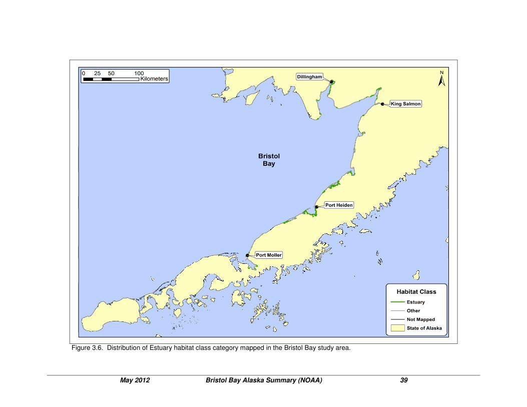
Further descriptions and definitions of the habitat class categories are presented in Appendix A, Tables A-11 and A-12. The occurrences of habitat class categories are summarized in Figure 3.5 and Table 3.2. Approximately 70% of all habitat class categories mapped are structured by wave energy, mostly in the mobile classes. Of the non-wave energy structured habitats, the Estuary habitat class is the most often observed, and accounts for 29% of the shoreline mapped so far in Bristol Bay. Fluvial processes are the dominant structuring force in this habitat class. The least common habitat class categories are those that are structured by current energy or are anthropogenic. Each of these classes account for approximately 1% or less of the shoreline mapped. The extent of Estuary habitat class mapped in Bristol Bay is shown in Figure 3.6.
Figure 3.5. Summary of habitat class categories mapped in the Bristol Bay study area
Habitat Class Current-
Dominated
1%Estuary
29%
Mobile
55%
Protected,
Partially
Mobile
11%
Semi-
Protected,
Immobile &
Partially
Mobile
2%
Semi-
Exposed,
Partially
Mobile
1%
Exposed,
Partially
Mobile
1%

May 2012 Bristol Bay Alaska Summary (NOAA) 38
Table 3.2. Summary of Habitat Class in Bristol Bay
Dominant Structuring
Process
Habitat Class Length (km) % of Mapping
Exposure Category Substrate Mobility
Wave Energy
Exposed (E)
Partially Mobile
18
1%
Semi-exposed (SE)
Partially Mobile
17
1%
Semi-protected (SP)
Immobile & Partially Mobile
26
2%
Protected (P)
Partially Mobile
179
11%
E, SE, SP, P
Mobile
892
55%
Fluvial/Estuarine processes
Estuary
473
29%
Current energy
Current dominated
10
1%
Man-modified
Anthropogenic
9
<1%
Lagoon *
Lagoon
147
9%
* Lagoons are classified as secondary habitat class Appendix A, Table A – 11.
May 2012 Bristol Bay Alaska Summary (NOAA) 39
Figure 3.6. Distribution of Estuary habitat class category mapped in the Bristol Bay study area.
May 2012 Bristol Bay Alaska Summary (NOAA) 40
4 REFERENCES
Berry, H.D., Harper, J.R., Mumford, T.F., Jr., Bookheim, B.E., Sewell, A.T., and Tamayo, L.J. 2004. Washington State ShoreZone Inventory User’s Manual, Summary of Findings, and Data Dictionary. Reports prepared for the Washington State Dept. of Natural Resources Nearshore Habitat Program. www.dnr.wa.gov/ResearchScience/Topics/Aquatic Habitats/Pages/aqr_nrsh_inventory_projects.aspx
Harney, J.N. 2007. Modeling Habitat Capability for the Non-Native European
Green Crab (Carcinus maenas) Using the ShoreZone Mapping System in Southeast Alaska, British Columbia, and Washington State. Report prepared for NOAA National Marine Fisheries Service (Juneau, AK). 75 p.
Harney, J.N. 2008. Evaluation of a Habitat Suitability Model for the Invasive
European Green Crab (Carcinus maenas) Using Species Occurrence Data from Western Vancouver Island, British Columbia. Report prepared for NOAA National Marine Fisheries Service (Juneau, AK). 51 p.
Harney, J.N., Morris, M., and Harper, J.R. 2008. ShoreZone Coastal Habitat
Mapping Protocol for the Gulf of Alaska. Report prepared for The Nature Conservancy, NOAA National Marine Fisheries Service, and the Alaska State Department of Natural Resources (Juneau, AK). 153 p.
Harper, J.R., and Morris, M.C. 2004. ShoreZone Mapping Protocol for the Gulf of
Alaska. Report prepared for the Exxon Valdez Oil Spill Trustee Council (Anchorage, AK). 61 p.
Howes, D., Harper, J.R., and Owens, E.H. 1994. Physical Shore-Zone Mapping
System for British Columbia. Report prepared by Environmental Emergency Services, Ministry of Environment (Victoria, BC), Coastal and Ocean Resources Inc. (Sidney, BC), and Owens Coastal Consultants (Bainbridge, WA). 71 p.
Howes, D.E. 2001. British Columbia biophysical ShoreZone mapping system – a
systematic approach to characterize coastal habitats in the Pacific Northwest. Puget Sound Research Conference, Seattle, Washington, Paper 3a, 11p.
Petersen, J., J. Michel, S. Zengel, M. White, C. Lord, C. Plank. 2002.
Environmental Sensitivity Index Guidelines. Version 3.0. NOAA Technical Memorandum NOS OR&R 11. Hazardous Materials Response Division, Office of Response and Restoration, NOAA Ocean Service, Seattle, Washington 98115 89p + App.

May 2012 Bristol Bay Alaska Summary (NOAA) 41
5 ACKNOWLEDGMENTS
The ShoreZone program is a partnership of scientists, GIS specialists, web specialists, non-profit organizations, and governmental agencies. We gratefully acknowledge the support of organizations working in partnership for the Alaska ShoreZone effort, including: Alaska Department of Fish and Game, Alaska Department of Natural Resources, Archipelago Marine Research Ltd., Coastal and Ocean Resources Inc., Cook Inlet Regional Citizens’ Advisory Council, Exxon Valdez Oil Spill Trustee Council, National Park Service, NOAA National Marine Fisheries Service, Prince William Sound Regional Citizens’ Advisory Council, The Nature Conservancy, United States Fish and Wildlife Service, the University of Alaska and the US Forest Service. We also thank the staff of Coastal and Ocean Resources Inc. and Archipelago Marine Research Ltd. for their efforts in the field and in the office. Protocols for data access and distribution are established by the program partner agencies. Please see www.ShoreZone.Org for a list of partner agencies and related web sites. Video imagery can be viewed and digital stills downloaded online at www.ShoreZone.Org. Any hardcopies or published data sets utilizing ShoreZone products shall clearly indicate their source. To ensure distribution of the most current public information or for correct interpretation, contact the ShoreZone project manager at Coastal and Ocean Resources, Inc. At the time of publication, that person is Dr. John Harper.

Appendix A
APPENDIX A DATA DICTIONARY
Table
Description
A-1 Definitions for fields and attributes in the UNIT table.
A-2 Definitions of the BC_CLASS attribute, in the UNIT table. (after Howes et al [1994] “BC Class” in British Columbia ShoreZone)
A-3 Definitions of the ESI (Environmental Sensitivity Index) attribute, from the UNIT table (after Peterson et al [2002]).
A-4 Definitions for estimating the OBSERVED PHYSICAL EXPOSURE attribute, (EXP_OBSER) in the UNIT table.
A-5 Definition of the OIL RESIDENCE INDEX (ORI) attribute in the UNIT table.
A-6 OIL RESIDENCE INDEX (ORI) Component lookup matrix based on exposure (columns) and substrate type (rows).
A-7 Definitions of the attributes in the BIOUNIT table.
A-8 Definitions of the BIOAREA attribute in BIOUNIT table.
A-9 List of the BIOLOGICAL WAVE EXPOSURE codes, in BIOUNIT table.
A-10 Definitions of BIOLOGICAL WAVE EXPOSURES, by bioband, and by indicator and associate species assemblages (EXP_BIO attribute in BIOUNIT table).
A-11 Expanded descriptions for HABITAT CLASS, SECONDARY HABITAT CLASS, and RIPARIAN fields of the BIOUNIT table.
A-12 Codes for HABITAT CLASS and SECONDARY HABITAT CLASS attributes, in the BIOUNIT table.
A-13 Definitions of fields and attributes in the XSHR (Across-shore) component table (after Howes et al 1994).
A-14 Definitions of FORM attributes, in XSHR (Across-shore) table (after Howes et al 1994).
A-15 Definitions of the MATERIALS attributes, in XSHR (Across-shore) table. (after Howes et al 1994).
A-16 Definitions for fields in the BIOBAND table. A-17 Definitions for BIOBAND attribute for Southeast Alaska, in BIOBAND
table. A-18 Definitions for Occurrences of Biobands, in the BIOBAND table. A-19 Definitions for fields in the PHOTOS table.

A-1
Table A-1. Definitions for Fields and Attributes in the UNIT table.
Field Name Description
UnitRecID Unit Record ID: An automatically-generated number field; the database “primary key” for unit-level relationships
PHY_IDENT
Physical Ident is a unique code to identify each unit, assigned by physical mapper; defined as an alphanumeric string determined by the codes for: Region, Area, Unit, and Subunit separated by slashes (e.g. 12/03/0552/0), where ‘12’ is Region 12, ‘03’ is Area 3, ‘0552’ is the Unit number, and ‘0’ is the Subunit number.
REGION Region: assigned during mapping, makes up first two digits of the PHY_IDENT. (See PHY_IDENT description for example.)
AREAS Area: assigned during mapping, makes up the third and fourth digits of the PHY_IDENT. (See PHY_IDENT description for example.)
PHY_UNIT Unit: Four digit along-shore unit number; assigned during mapping, unique within Region/Area mapping section. (See PHY_IDENT description for example.)
SUBUNIT
Subunit: assigned during mapping, is ‘0’ for unit line features. Subunit field is used to identify Point features (if any, also called ‘Variants’) within Units, and are numbered sequentially (1, 2, 3…) according to the order occurring within the unit. (See PHY_IDENT description for example.)
TYPE Unit Type: A single-letter description for Unit as either: a (L)ine (linear unit) or (P)oint feature (variant). Related to SUBUNIT attribute, where each numbered SUBUNIT ‘variant’ would be TYPE ‘P’
BC_CLASS
BC Coastal Class: Code number for Coastal Class classification for the unit. Definitions of codes in Table A-2. Determined by the Physical mapper and based on: overall substrate type, sediment size (if sediment is present), across-shore width, and across-shore slope for the unit; derived from the Howes et al (1994)
ESI Environmental Sensitivity Index Classification for the shore unit, using unit-wide interpretation of ESI. Definitions in Table A-3, after Peterson et al [2002].
LENGTH_M Unit Length: Along-shore unit high waterline, in meters; calculated in ArcGIS, from digitized shoreline
GEO_MAPPER Physical Mapper Name: Last name of the physical mapper
GEO_EDITOR Physical Mapper Reviewer: Last name of the physical mapper who QA/QCs the work (10% of all units are reviewed by a different Physical mapper than did original mapping)
VIDEOTAPE
Videotape Name: Unique code for title of the videotape used for mapping; Naming convention example is SE07_SO_08, where first four characters identify the main survey region and year, (where SE07 is ‘Southeast Alaska 2007’), two letter code for survey team (where SO is ‘Sockeye’) and two digit code ‘08’ is for consecutively numbered tape.
HR Hour: From the first two digits of the 6-digit UTC time burned on video image, identifying video frame at which the unit starts; with the unit start frame at center of viewing screen
MIN Minute: From the third and fourth digits of the 6-digit UTC time burned on video image at which unit starts; with the unit start frame at center of viewing screen
SEC Seconds: From the last two digits of the 6-digit UTC time burned on video image at which unit starts; with the unit start frame at center of viewing screen
EXP_OBSER Physical wave exposure: Estimate of wave exposure as observed by the physical mapper, estimated from observed fetch and coastal processes; categories listed in Table A-4.
[continued]

A-2
Table A-1. Definitions for Fields and Attributes in the UNIT table. (continued)
Field Name Description
ORI Oil Residency Index: Code indicating the potential persistence of oil within the shore unit. Based on unit substrate type and biological wave exposure categories. Definitions and lookup matrix in Tables A-5 and A-6
SED_SOURCE Sediment Source: Code to indicate estimated sediment source for the unit: (A)longshore, (B)ackshore, (F)luvial, (O)ffshore, (X) not identifiable
SED_ABUND Sediment Abundance: Code to indicate the relative sediment abundance within the shore-unit: (A)bundant, (M)oderate, (S)carce
SED_DIR
Sediment Transport Direction: One of the eight cardinal points of the compass indicating dominant sediment transport direction (N, NE, E, SE, S, SW, W, NW). (X) Indicates transport direction could not be discerned from imagery.
CHNG_TYPE Change Type: Code indicating the estimated stability of the shore unit, reflecting the relative degree of “measurable change” during a 3-5 year time span: (A)ccretional, (E)rosional, (S)table
SHORENAME Shorename: Name of a prominent geographic feature near the unit (from nautical chart or gazetteer)
UNIT_COMMENTS Unit Comments: Text field for comments and notes during physical mapping
SM1_TYPE
Primary Shore Modification: 2-letter code indicating the primary type of shore modification occurring within the unit: BR = boat ramp; CB = concrete bulkhead; LF = landfill; SP= sheet pile; RR = rip rap and WB = wooden bulkhead
SM1_PCT Primary Shore Modification Percent Unit Length: Estimated % occurrence of the primary shore modification type in tenths (i.e. “2” = 20% occurrence with the unit alongshore)
SM2_TYPE Secondary Shore Modification: 2-letter code indicating the secondary type of shore modification occurring within the unit
SM2_PCT Secondary Shore Modification Percent Unit Length: Estimated % occurrence of the secondary type of shore modification occurring within the unit
SM3_TYPE Tertiary Shore Modification: 2-letter code indicating the tertiary type of shore modification occurring within the unit
SM3_PCT Tertiary Shore Modification Percent Unit Length: Estimated % occurrence of the tertiary seawall type in tenths (i.e., “2” = 20% occurrence within the unit)
SMOD_TOTAL Total Shore Modification % Unit Length: Total % occurrence of shore modification in the unit in tenths
RAMPS Boat Ramps: Number of boat ramps that occur within the unit; ramps must impact some portion of the shore-zone and generally be constructed of concrete, wood or aggregate
PIERS_DOCK Piers or Wharves: Number of piers or wharves that occur within the unit; piers or docks must extend at least 10 m into the intertidal zone; does not include anchored floats
REC_SLIPS Dock Slips: Estimated number of recreational slips at docks or marinas within the unit; based on small boat length ~<50’
DEEPSEA_SLIP Ship Dock Slips: Estimated number of slips for ocean-going vessels within the unit; based on ship length ~>100’
ITZ Intertidal Zone Width: Sum of the across-shore width of all the intertidal (B Zone) components within the unit
SLIDE Still Photo in Unit: Yes/No tick box to indicate if high resolution photo is available for the Unit.
EntryDate ModifiedDate
Date/Time Mapped or Modified: Date and time the unit was physically mapped (or modified)

A-3
Table A-2. Definitions of the BC_CLASS attribute, in the UNIT table. (after Howes et al [1994] “BC Class” in British Columbia ShoreZone)
Substrate Sediment Width Slope BC_CLASS
Description CODE
Rock n/a
Wide (>30 m)
Steep (>20°)
n/a -
Inclined (5-20°)
Rock Ramp, wide 1
Flat (<5°) Rock Platform, wide 2
Narrow (<30 m)
Steep (>20°)
Rock Cliff 3
Inclined (5-20°)
Rock Ramp, narrow 4
Flat (<5°) Rock Platform, narrow 5
Rock & Sediment
Gravel
Wide (>30 m)
Steep (>20°)
n/a -
Inclined (5-20°)
Ramp with gravel beach, wide
6
Flat (<5°) Platform with gravel beach, wide
7
Narrow (<30 m)
Steep (>20°)
Cliff with gravel beach 8
Inclined (5-20°)
Ramp with gravel beach 9
Flat (<5°) Platform with gravel beach 10
Sand & Gravel
Wide (>30 m)
Steep (>20°)
n/a -
Inclined (5-20°)
Ramp w gravel & sand beach, wide
11
Flat (<5°) Platform with G&S beach, wide
12
Narrow (<30 m)
Steep (>20°)
Cliff with gravel/sand beach 13
Inclined (5-20°)
Ramp with gravel/sand beach
14
Flat (<5°) Platform with gravel/sand beach
15
Sand
Wide (>30 m)
Steep (>20°)
n/a -
Inclined (5-20°)
Ramp with sand beach, wide
16
Flat (<5°) Platform with sand beach, wide
17
Narrow (<30 m)
Steep (>20°)
Cliff with sand beach 18
Inclined (5-20°)
Ramp with sand beach, narrow
19
Flat (<5°) Platform with sand beach, narrow
20
Sediment
Gravel
Wide (>30 m)
Flat (<5°) Gravel flat, wide 21
Narrow (<30 m)
Steep (>20°)
n/a -
Inclined (5-20°)
Gravel beach, narrow 22
Flat (<5°) Gravel flat or fan 23
Sand & Gravel
Wide (>30 m)
Steep (>20°)
n/a -
Inclined (5-20°)
n/a -
Flat (<5°) Sand & gravel flat or fan 24
Narrow (<30 m)
Steep (>20°)
n/a -
Inclined (5-20°)
Sand & gravel beach, narrow
25
Flat (<5°) Sand & gravel flat or fan 26
Sand/Mud
Wide (>30 m)
Steep (>20°)
n/a -
Inclined (5-20°)
Sand beach 27
Flat (<5°) Sand flat 28
Flat (<5°) Mudflat 29
Narrow (<30 m)
Steep (>20°)
n/a -
Inclined (5-20°)
Sand beach 30
Flat (<5°) n/a -
Organics n/a n/a Organics 31
Anthropogenic Man-made n/a n/a Man-made, permeable 32
n/a Man-made, impermeable 33
Channel Current n/a n/a Channel 34
Glacier Ice n/a n/a Glacier 35
Lagoon n/a n/a n/a Lagoon 36

A-4
Table A-3. Definitions of the ESI (Environmental Sensitivity Index) attribute, from the UNIT table. (after Peterson et al [2002])
Environmental Sensitivity Index (ESI)
CODE Description
1A Exposed rocky shores; exposed rocky banks 1B Exposed, solid man-made structures 1C Exposed rocky cliffs with boulder talus base 2A Exposed wave-cut platforms in bedrock, mud, or clay 2B Exposed scarps and steep slopes in clay 3A Fine- to medium-grained sand beaches 3B Scarps and steep slopes in sand 3C Tundra cliffs 4 Coarse-grained sand beaches 5 Mixed sand and gravel beaches
6A Gravel beaches; Gravel Beaches (granules and pebbles 6B Gravel Beaches (cobbles and boulders) 6C Rip rap (man-made) 7 Exposed tidal flats
8A Sheltered scarps in bedrock, mud, or clay; Sheltered rocky shores (impermeable) 8B Sheltered, solid man-made structures; Sheltered rocky shores (permeable) 8C Sheltered rip rap 8D Sheltered rocky rubble shores 8E Peat shorelines 9A Sheltered tidal flats 9B Vegetated low banks 9C Hypersaline tidal flats 10A Salt- and brackish-water marshes 10B Freshwater marshes 10C Swamps 10D Scrub-shrub wetlands; mangroves 10E Inundated low-lying tundra
Table A-4. Definitions for estimating the OBSERVED PHYSICAL EXPOSURE attribute, (EXP_OBSER) in the UNIT table.
Maximum Fetch (km)
Modified Effective Fetch (km)
<1 1 - 10 10 - 50 50 - 500 >500
<1 very protected n/a n/a n/a n/a
<10 protected protected n/a n/a n/a 10 – 50 n/a semi-protected semi-protected n/a n/a
50 – 500 n/a semi-exposed semi-exposed semi-exposed n/a >500 n/a n/a semi-exposed exposed exposed
Codes for exposures: Very Protected = VP; Protected = P; Semi-Protected =SP; Semi-Exposed = SE; Exposed = E; Very Exposed = VE

A-5
Table A-5. Definition of the OIL RESIDENCE INDEX (ORI) attribute in the UNIT table.
Persistence Oil Residence Index (ORI) Estimated Persistence
Short 1 Days to weeks
Short to Moderate 2 Weeks to Months
Moderate 3 Weeks to Months
Moderate to Long 4 Months to Years
Long 5 Months to Years
Table A-6. OIL RESIDENCE INDEX (ORI) Component lookup matrix based on exposure (columns) and substrate type (rows). Component Substrate VE E SE SP P VP
rock 1 1 1 2 3 3
man-made, impermeable 1 1 1 2 2 2
boulder 2 3 5 4 4 4
cobble 2 3 5 4 4 4
pebble 2 3 5 4 4 4
sand with pebble, cobble or boulder
1 2 3 4 5 5
sand without pebble, cobble or boulder
2 2 3 3 4 4
mud 999 999 999 3 3 3
organics/vegetation 999 999 999 5 5 5
man-made, permeable 2 2 3 3 5 5

A-6
Table A-7. Definitions of the attributes in the BIOUNIT table.
Field Name Code Description
UnitRecID Unit Record ID: Automatically-generated number field; the database “primary key” required for relationships between tables
PHY_IDENT
Physical_Ident is a unique code to identify each unit, assigned by physical mapper; defined as an alphanumeric string determined by the codes for: Region, Area, Unit, and Subunit separated by slashes (e.g. 12/03/0552/0), where ‘12’ is Region 12, ‘03’ is Area 3, ‘0552’ is the Unit number, and ‘0’ is the Subunit number.
BIOAREA Bioarea: Geographic division used to describe regional differences in observed biota and coastal habitats (Bioarea codes and descriptions listed in Table A-8)
EXP_BIO Biological Wave Exposure: A classification of the wave exposure category within the Unit. In Bristol Bay: assigned by the Biological mapper, based on physical wave exposure category [EXP_ OBSER]
HAB_CLASS
Habitat Class: Code for a classification of overall habitat category within the Unit, assigned by the biological mapper. Based on the Biological Exposure (EXP_BIO) and the geomorphic features of the shoreline (Table A-11 and A-12). (In Bristol Bay EXP_BIO = EXP_OBSER)
HAB_CLASS_LTRS Habitat Class in alphabetic code: translation from number codes in the HAB CLASS lookup table (Table A-12)
HAB_OBS Habitat Observed: Original Habitat code categories used to classify Habitat Type; not used in current protocol but kept for backward-compatibility with earlier projects; replaced by HAB_CLASS
BIO_SOURCE Biomapping Source: The source data used to interpret coastal zone biota: (V)ideotape, (V2) - lower quality video imagery, (S)lide, (I)nferred
HAB_CLASS2
Secondary Habitat Class: Code for a classification of secondary Lagoon-type habitat within the Unit, assigned by the biological mapper. Based on the Biological Exposure (EXP_BIO) and lagoon habitat types (Table A-11 and A-12)
HC2_SOURCE
Secondary Habitat Class Source: Source used to interpret the Secondary Habitat Class (HAB_CLASS2) “lagoon”: OBServed as viewed from video, LooKUP referring to ‘Form’ Code (Table A-11 and Table A-12) Lo or Lc in across-shore physical component table (Table A-13 and A-14)
HC2_Note Secondary Habitat Class Comment: comment field for Secondary Habitat Class ((HAB_CLASS2))
RIPARIAN_PERCENT
Riparian Percent Overhang: Estimate of the percentage of alongshore length of the intertidal zone, in which the shoreline is shaded by overhanging riparian vegetation; all substrate types (Expanded definition in Table A-11)
RIPARIAN_M
Riparian Overhang Meters: Calculated portion of the unit length, in meters, of riparian overhang in the intertidal (B) zone, using LENGTH_M field of UNIT table, and RIPARIAN_PERCENT of BIOUNIT table; all substrate types;
BIO_UNIT_COMMENT Biological Comments: regarding the along-shore unit as a whole. Included as deliverable data, as note format.
BIO_MAPPER Biological Mapper: The initials of the biological mapper that provided the biological interpretation of the imagery
PHOTO Still Photo in Unit: Yes/No tick box to indicate if high resolution photo is available for the Unit. (see BIOSLIDE table)
DateAdded DateModified
Date/Time Mapped or Modified: Date and time the unit was physically mapped (or modified)

A-7
Table A-8. Definitions of the BIOAREA attribute in BIOUNIT table. Bioarea Name
Bioarea Code
Bioarea Suffix *
Geographic Extent Characteristics
Outer Kenai KENA 8
Kenai Coast, Alaska, including Kenai Fjords National Park, from Cape Elizabeth at the east entrance of Cook Inlet to Port Bainbridge at the west entrance of Prince William Sound.
Rugged coastline, dominated by extremely steep shores and Very Exposed wave energy. Fjord heads with tidewater glaciers. Absence of Dragon Kelp and Giant Kelp biobands.
Cook Inlet COOK 9
Cook Inlet, Alaska, from Cape Douglas on the southwest entrance Cook Inlet, north to Anchorage, including Turnagain Arm and Kachemak Bay, to Cape Elizabeth at the southeast entrance of Cook Inlet.
Sediment-dominated, wide, low-slope shorelines, moderate to lower wave exposures. Affected by silt-laden freshwater input, absence of Giant Kelp and Dragon Kelp. Very wide complexes of salt marshes and estuaries.
Kodiak Island
KODI 10
Kodiak archipelago, Gulf of Alaska side, from Tugidak Island and Akhiok at the southwest end of the archipelago, to Shuyak Island at the northeast end of the islands.
Diversity of habitats and wave exposures, from Very Protected estuaries to Exposed rock cliffs. Fully marine and open to Gulf of Alaska. Lush lower intertidal brown algae, red algae and canopy kelps, in particular at north end. Southwest coast has wide rock platforms with surfgrass beds and sediment dominated offshore islands.
Katmai / Shelikof Strait side of Kodiak Island
KATM 11
Katmai National Park and Preserve, Alaska Peninsula, Shelikof Strait, includes the northwest side of the Kodiak archipelago.
Moderate to high wave exposures, affected by outflow from Cook Inlet, and separated from open Gulf of Alaska by Kodiak archipelago. Limited diversity of lower intertidal browns and canopy kelps, with diversity of red algae characterizing higher exposure sites. Includes both coasts of Shelikof Strait.
Aniakchak ANIA 11 Aniakchak National Monument and Preserve, Alaska Peninsula, Shelikof Strait, southwest of Katmai National Park.
High wave exposure, wide bedrock platforms and mobile sediment beaches. Included in KATM bioareas for species descriptions, pending further delineation of bioarea boundaries. Likely transitional to Aleutian bioareas.
Southeast Alaska -- Yakutat
SEYA 12
The Yakutat region, on the Gulf of Alaska coast. Extends from the outer edge of the Copper River delta, near Cordova, south through Yakutat Bay, to Icy Point, just north of Cross Sound.
Exposed west-facing coast, open to Gulf of Alaska. Mobile, high-energy sediment beaches dominant. Limited canopy kelp distribution.
Southeast Alaska – Lynn Canal (fjord)
SEFJ 12
Lynn Canal from Point Howard at the southwest edge, at SEIC boundary, north to Skagway, and the east side of Lynn Canal south. Includes Juneau, Douglas Island, Taku Inlet and Port Snettisham with the southeast edge to the south tip of Glass Peninsula, Hugh Point on Admiralty Island.
Fjord landscape, bedrock dominated, moderate to low wave exposures, glacial silty waters. Low species diversity in intertidal, dense Blue Mussel bioband, absence of Dragon Kelp and Giant Kelp biobands.
* Suffix applied to four lower intertidal biobands (HAL, RED, SBR, CHB) to distinguish between regional differences in species composition of these bands in different bioareas.
[continued]

A-8
Table A-8. Definitions of the BIOAREA attribute in BIOUNIT table. (continued) Bioarea Name
Bioarea Code
Bioarea Suffix *
Geographic Extent Characteristics
Southeast Alaska – Icy Strait
SEIC 12
The Icy Strait region, of northern SE Alaska. The north extend is at Icy Point, at SEYA boundary, south to Cape Spencer and the north shore Cross Sound, east to the southwest entrance of Lynn Canal at Point Howard. Includes entire south shore Icy Strait, from Point Lucan at west to False Bay, northeast Chichagof Island.
Glacial silty water, wide, sediment-dominated beaches common, fringing salt marsh common, moderate and lower wave exposures, wide estuary flats common. Dragon Kelp dominant canopy kelp.
Southeast Alaska – Sitka
SESI 12
The Sitka area includes the northwest sides of Chichagof and Baranof Islands. The northern boundary is at Point Lucan in Icy Strait, including Yakobi and Kruzof Islands with the southern boundary at the southern tip of Baranof Island at Cape Ommaney.
Fully marine, west coast, includes diversity of species, exposure and habitat categories, from Exposed to Very Protected. Giant Kelp abundant, Dragon Kelp limited distribution.
Southeast Alaska – Misty Fjords
SEMJ 12
Misty Fjords area includes all fjords in the southeast region of Southeast Alaska, including Behm Canal, George Inlet, Carroll Inlet, Thorne Arm, Boca de Quadra and the western side of Portland Inlet.
Fjord landscape, bedrock-dominated, low wave exposures. Low species diversity. Absence of Giant Kelp and Dragon Kelp.
Southeast Alaska – Craig
SECR 12
The Craig area includes islands in the southwest region of Southeast Alaska, including areas around Ketchikan as well as Prince of Wales Island, Dall Island and all surrounding archipelagos, from southern Coronation Island, south to Dixon Entrance.
Fully marine, west coast. High species diversity and habitat heterogeneity. Northern limit of California Mussel and Urchin Barrens biobands and certain species of other lower intertidal kelps. Southern limit of Dragon Kelp.
Southeast Alaska -- Stikine
SESK 12
The Stikine area encompasses central Southeast Alaska. Northern extent includes east Chichagof Island from False Bay, west Admiralty Island and south from Tracy and Endicott Arms. Includes east Baranof, Kuiu and Kupreanof Islands as well as the Stikine River and surrounding Islands, Etolin and Wrangell. Southern boundary crosses Coronation and Warren Islands and northwest Prince of Wales Island
Glacial silty water affected, diversity of shoreline habitats and substrate types, moderate and lower wave exposures. Dragon Kelp dominant canopy kelp.
Prince William Sound
PRWS 13
All of Prince William Sound from Orca Inlet at Cordova on the east, to the south end of Montague Island, and across to Port Bainbridge on the west.
Diverse habitat, with high Semi-Exposed to Very Protected wave exposures. Differences between conditions in eastern and western Sound, with interaction of circulation complexities. Numerous tidewater glaciers and affects of Copper River. Absence of Giant Kelp and Dragon Kelp.
Bristol Bay BRIS 16 False Pass, Bechevin Bay to Cape Newenham
Wide sand and mud flats, braided stream and river mouths, dominated by mobile beaches, with few areas of immobile substrate.
* Suffix applied to four lower intertidal biobands (HAL, RED, SBR, CHB) to distinguish between regional differences in species composition of these bands in different bioareas.

A-9
Table A-9. List of the BIOLOGICAL WAVE EXPOSURE codes, in BIOUNIT table. Biological Wave Exposure
Name Code
Very Exposed VE
Exposed E
Semi-Exposed SE
Semi-Protected SP
Protected P
Very Protected VP
Table A-10. Definitions of BIOLOGICAL WAVE EXPOSURES, by bioband, and by indicator and associate species assemblages (EXP_BIO attribute in BIOUNIT table).
Exposure Zone Indicator Species Associated Species Bioband Name Bioband
Code
Ve
ry E
xp
ose
d (
VE
) &
Exp
ose
d (
E)
Up
pe
r In
tert
ida
l
Leymus mollis Dune Grass GRA Verrucaria Splash Zone VER
Balanus glandula Semibalanus balanoides
Barnacle BAR
Semibalanus cariosus Barnacle BAR Mytilus trossulus Blue Mussel BMU
Lo
we
r In
tert
ida
l &
N
ea
rsh
ore
Sub
tida
l Mytilus californianus California Mussel MUS
Coralline red algae Red Algae RED
Alaria ‘nana’ morph Alaria ALA
Lessoniopsis littoralis Dark Brown Kelps CHB
Laminaria setchellii Dark Brown Kelps CHB
Nereocystis luetkeana Bull Kelp NER
Se
mi-
Ex
po
se
d (
SE
)
Up
pe
r In
tert
ida
l
Leymus mollis Dune Grass GRA Verrucaria Splash Zone VER
Balanus glandula Semibalanus balanoides
Barnacle BAR
Fucus distichus Rockweed FUC Semibalanus cariosus Barnacle BAR Mytilus trossulus Blue Mussel BMU
Lo
we
r In
tert
ida
l &
N
ea
rsh
ore
Sub
tida
l
mixed filamentous and foliose red algae
Red Algae RED
Alaria ‘marginata’ morph Alaria ALA Phyllospadix sp. Surfgrass SUR Laminaria setchellii Dark Brown Kelps CHB Saccharina subsimplex Dark Brown Kelps CHB Saccharina sessile smooth morph
Dark Brown Kelps CHB
Alaria fistulosa Dragon Kelp ALF
Strongylocentrous
fransciscanus Urchin Barrens URC
Macrocystis integrifolia Giant Kelp MAC Nereocystis luetkeana Bull Kelp NER
[continued]

A-10
Table A-10. Definitions of BIOLOGICAL WAVE EXPOSURES, by bioband, and by indicator and associate species assemblages (EXP_BIO attribute in BIOUNIT table).(continued)
Exposure Zone Indicator Species Associated Species Bioband Name Bioband
Code S
em
i-P
rote
cte
d (
SP
)
Up
pe
r In
tert
ida
l
Leymus mollis Dune Grass GRA Carex spp. Sedges SED Puccinellia sp. Salt Marsh PUC Plantago maritima Salt Marsh PUC Glaux maritima Salt Marsh PUC Verrucaria Splash Zone VER
Lo
we
r In
tert
ida
l &
N
ea
rsh
ore
Sub
tida
l
Balanus glandula Semibalanus balanoides
Barnacle BAR
Semibalanus carriosus Barnacle BAR Fucus distichus Rockweed FUC Mytilus trossulus Blue Mussel BMU Ulva spp. Green Algae ULV
Bleached mixed red algae Bleached Red Algae
HAL
Mixed red algae including Odonthalia
Red Algae RED
Alaria ‘marginata’ morph Alaria ALA Zostera marina Eelgrass ZOS Saccharina latissima Soft Brown Kelps SBR Nereocystis luetkeana Bull Kelp NER Macrocystis integrifolia Giant Kelp MAC
Pro
tec
ted
(P
) &
V
ery
Pro
tec
ted
(V
P)
Up
pe
r In
tert
ida
l
Leymus mollis Dune Grass GRA Carex spp. Sedges SED Puccinellia sp. Salt Marsh PUC Plantago maritima Salt Marsh PUC Glaux maritima Salt Marsh PUC Verrucaria Splash Zone VER
Balanus glandula Semibalanus balanoides
Barnacle BAR
Fucus distichus Rockweed FUC Mytilus trossulus Blue Mussel BMU
Lo
we
r In
tert
ida
l &
N
ea
rsh
ore
Sub
tida
l
Ulva spp. Green Algae ULV
Zostera marina Eelgrass ZOS
Saccharina latissima Soft Brown Kelps SBR

A-11
Table A-11. Expanded descriptions for HABITAT CLASS, SECONDARY HABITAT CLASS, and RIPARIAN fields of the BIOUNIT table.
Attribute Description
HAB_CLASS
Habitat Class attribute is a classification of the biophysical characteristics of an entire unit, and provides a single attribute that describes the typical intertidal biota and the associated biological wave exposure together with the geomorphology. That is, a typical example of a Habitat Class includes a combination of biobands, and their associated indicator species (which determine the Biological Exposure category) and the geomorphological features of the Habitat Class. The biological mapper observes and records the biobands in the unit, if any, and determines the Biological Exposure Category (EXP_BIO). The Habitat Class is determined on the basis of presence/absence of biobands, exposure category, geomorphology, and spatial distribution of biota within the unit. Within the database, both a numeric code and an alpha code are used. Both codes for Habitat Class are listed in Table A-12, in which the matrix includes all combinations of Dominant Structuring Process, with associated substrate mobility and general geomorphic type on the vertical axis, and Biological Exposure on the horizontal axis.
HAB_CLASS2
The ‘Secondary Habitat Class’ was added as an attribute in the BioUnit Table during biological mapping of the Kodiak Archipelago in order to specifically identify lagoon habitats. Many backshore lagoons were observed in the Kodiak region, and they represent an unusual coastal habitat that differs from other estuaries and marshes. Units classified as lagoons contain brackish or salt water contained in a basin with limited drainage. They are often associated with wetlands and may include wetland biobands in the upper intertidal. Single units classified as lagoons often have the lagoon form in the A zone; however, some lagoons are large and may encompass several units when the lagoon form is mapped as the C zone.
RIPARIAN_PERCENT
As an attribute in the BIOUNIT table, the Riparian_Percent value is intended to be an index for the potential habitat for upper beach spawning fishes. The value recorded in the Riparian_Percent field is an estimate of the percentage of the unit’s total alongshore length in which riparian vegetation (trees and shrubs) shades the upper intertidal zone. Shading of the highest high water line is a good estimate of riparian shading; therefore, shading of wetland herbs and grasses is not included in the estimate, nor is any shading of the splash zone alone. Shading must be visible in the upper intertidal zone, and the shading vegetation must be woody trees or shrubs. Riparian overhanging vegetation is also an indicator of lower wave exposures, in which the splash zone is narrow. Shading may occur in on sediment-dominated or in rocky intertidal settings.

A-12
Table A-12. Codes for HABITAT CLASS and SECONDARY HABITAT CLASS attributes, in the BIOUNIT table.
Dominant Structuring
Process
Substrate Mobility
Coastal Type
Description
Biological Exposure Category
Very Exposed
(VE)
Exposed
(E)
Semi-Exposed
(SE)
Semi-Protected
(SP)
Protected
(P)
Very Protected
(VP)
Wave energy
Immobile
Rock or Rock & Sediment or Sediment
The epibiota in the immobile mobility categories is influenced by the wave exposure at the site. In high wave exposures, only solid bedrock shorelines will be classified as ‘immobile’. At the lowest wave exposures, even pebble/cobble beaches may show lush epibiota, indicating an immobile Habitat Class.
10 VE_I
20 E_I
30 SE_I
40 SP_I
50 P_I
60 VP_I
Partially Mobile
Rock & Sediment or Sediment
These units describe the combination of sediment mobility observed. That is, a sediment beach that is bare in the upper half of the intertidal with biobands occurring on the lower beach would be classed as ‘partially mobile’. This pattern is seen at moderate wave exposures. Units with immobile bedrock outcrops intermingled with bare mobile sediment beaches, as can be seen at higher wave exposures, could also be classified as ‘partially mobile’.
11 VE_P
21 E_P
31 SE_P
41 SP_P
51 P_P
61 VP_P
Mobile Sediment
These categories are intended to show the ‘bare sediment beaches’, where no epibenthic macrobiota are observed. Very fine sediment may be mobile even at the lowest wave exposures, while at the highest wave exposures; large-sized boulders will be mobile and bare of epibiota.
12 VE_M
22 E_M
32 SE_M
42 SP_M
52 P_M
62 VP_M
Fluvial/ Estuarine processes
Estuary
Units classified as the ‘estuary’ types always include salt marsh vegetation in the upper intertidal, are always associated with a freshwater stream or river and often show a delta form. Estuary units are usually in lower wave exposure categories.
13 VE_E
23 E_E
33 SE_E
43 SP_E
53 P_E
63 VP_E
Current energy
Current-Dominated
Species assemblages observed in salt-water channels are structured by current energy rather than by wave energy. Current-dominated sites are limited in distribution and are rare habitats.
14 VE_C
24 E_C
34 SE_C
44 SP_C
54 P_C
64 VP_C
Glacial processes
Glacier In a few places in coastal Alaska, saltwater glaciers form the intertidal habitat. These Habitat Classes are rare and include a small percentage of the shoreline length.
15 VE_G
25 E_G
35 SE_G
45 SP_G
55 P_G
65 VP_G
Anthropogenic
Anthropogenic – Impermeable
Impermeable modified Habitats are intended to specifically note units classified as Coastal Class 33. These Habitat Classes are rare and include a small percentage of the shoreline length.
16 VE_X
26 E_X
36 SE_X
46 SP_X
56 P_X
66 VP_X
Anthropogenic – Permeable
Permeable modified Habitats are intended to specifically note shore units classified as Coastal Class 32. These Habitat Classes are rare and include a small percentage of the shoreline length.
17 VE_Y
27 E_Y
37 SE_Y
47 SP_Y
57 P_Y
67 VP_Y
Lagoon
Lagoon
Units classified as Lagoons in the Secondary Habitat Class contain brackish or salty water that is contained within a basin that has limited drainage. They are often associated with wetlands and may include wetland biobands in the upper intertidal.
18 VE_L
28 E_L
38 SE_L
48 SP_L
58 P_L
68 VP_L
Shaded boxes are not applicable in most regions

A-13
Table A-13. Definitions of fields and attributes in the XSHR (Across-shore) component table. (after Howes et al 1994)
Field Name Description
UnitRecID Unit Record ID: An automatically-generated number field; the database “primary key” for unit-level relationships
XshrRecID Across-shore Record ID: Automatically-generated number field; the database “primary key” for across-shore relationships
PHY_IDENT Physical Ident is a unique code to identify each unit, assigned by physical mapper; defined as an alphanumeric string determined by the codes for: Region, Area, Unit, and Subunit separated by slashes (e.g. 12/03/0552/0
CROSS_LINK Crosslink code: Unique identifier for each across-shore record, consisting of an alphanumeric string comprised of the PHY_IDENT followed by the Zone and Component separated by slashes (e.g. 12/03/0552/0/A/1)
ZONE Across-shore Zone: Code indicating the across-shore position (tidal elevation) of the Component: (A) supratidal, (B) intertidal, (C) subtidal
COMPONENT Across-shore Component: a subdivision of Zones, numbered from highest to lowest elevation in across-shore profile (e.g. A1 is the highest supratidal component; B1 is the highest intertidal; B2 is lower intertidal)
Form1 Form1: The principal geomorphic feature within across-shore Component, described by a specific set of codes (Table A-11)
MatPrefix1 Material Prefix: Veneer indicator field; blank = no veneer; “v” = veneer
Mat1 Material (substrate and/or sediment type) that best characterizes Form1, described by a specific set of codes (Table A-12)
FormMat1Txt Form/Material Text: Automatically-generated field that is the translation of codes used in Form1 and Mat1 into text
Form2 Form2: Secondary geomorphic feature within across-shore Component, described by a specific set of codes (Table A-11)
MatPrefix2 Material Prefix: Veneer indicator field; blank = no veneer; “v” = veneer
Mat2 Material (substrate and/or sediment type) that best characterizes Form2, described by a specific set of codes (Table A-12)
FormMat2Txt Form/Material Text: Automatically-generated field that is the translation of codes used in Form2 and Mat3 into text
Form3 Form3: Tertiary geomorphic feature within each across-shore component, described by a specific set of codes (Table A-11)
MatPrefix3 Material Prefix: Veneer indicator field; blank = no veneer; “v” = veneer
Mat3 Material (substrate and/or sediment type) that best characterizes Form3, described by a specific set of codes (Table A-12)
FormMat3Txt Form/Material Text: Automatically-generated field that is the translation of codes used in Form3 and Mat3 into text
Form4 Form4: Fourth-order geomorphic feature within each across-shore component, described by a specific set of codes (Table A-11)
MatPrefix4 Material Prefix: Veneer indicator field; blank = no veneer; “v” = veneer
Mat4 Material (substrate and/or sediment type) that best characterizes Form4, described by a specific set of codes (Table A-12)
FormMat4Txt Form/Material Text: Automatically-generated field that is the translation of codes used in Form4 and Mat4 into text
WIDTH Width: Estimated mean across-shore width of the component (e.g. A1) in meters
SLOPE Slope: Estimated across-shore slope of the mapped geomorphic Form in degrees; must be consistent with Form codes (Table A-11)
PROCESS Coastal Process dominant in affecting the morphology: (F)luvial, (M)ass wasting (landslides), (W)aves, (C)urrents, (E)olian (wind, as with dunes) (O)ther
COMPONENT_ORI Component Oil Residence Index on the basis of substrate type; 1 is least persistent, 5 is most persistent (Tables A-5 and A-6)

A-14
Table A-14. Definitions of FORM attributes, in XSHR (Across-shore) table. (after Howes et al 1994) A = Anthropogenic
a pilings, dolphin b breakwater c log dump d derelict shipwreck f float g groin i cable/ pipeline j jetty k dyke m marina n ferry terminal o log booms p port facility q aquaculture r boat ramp s seawall t landfill, tailings w wharf x outfall or intake y intake
B = Beach
b berm (intertidal or supratidal)
c washover channel f face i inclined (no berm) m multiple bars / troughs n relic ridges, raised p plain r ridge (single bar; low to
mid intertidal) s storm ridge (occas
marine influence; supratidal)
t low tide terrace v thin veneer over rock
(also use as modifier) w washover fan
C = Cliff
stability/geomorphology a active/eroding p passive (vegetated) c cave slope i inclined (20°-35°) s steep (>35°) [continued]
Cliff continued
height l low (<5m) m moderate (5-10m) h high (>10m) modifiers (optional) f fan, apron, talus g surge channel t terraced r ramp
D = Delta
b bars f fan l levee m multiple channels p plain (no delta, <5°) s single channel
E = Dune
b blowouts i irregular n relic o ponds r ridge/swale p parabolic v veneer w vegetated
F = Reef
(no vegetation) f horizontal (<2°) i irregular r ramp s smooth
I = Ice g glacier
L = Lagoon o open c closed
M = Marsh
c tidal creek e levee f drowned forest h high l mid to low
(discontinuous) o pond s brackish, supratidal
O = Offshore Island
(not reefs) b barrier c chain of islets t table shaped p pillar/stack w whaleback elevation l low (<5m) m moderate (5-10m) h high (>10m)
P = Platform
(slope <20°) f horizontal g surge channel h high tide platform i irregular l low tide platform r ramp (5-19°) t terraced s smooth p tidepool
R = River Channel
a perennial i intermittent m multiple channels s single channel
T = Tidal Flat
b bar, ridge c tidal channel e ebb tidal delta f flood tidal delta l levee p tidepool s multiple tidal channels t flats

A-15
Table A-15. Definitions of the MATERIALS attributes, in XSHR (Across-shore) table. (after Howes et al 1994) A = Anthropogenic
a metal (structural) c concrete (loose blocks) d debris (man-made) f fill, undifferentiated mixed o concrete (solid cement blocks) r rubble, rip rap t logs (cut trees) w wood (structural)
B = Biogenic
c coarse shell f fine shell hash g grass on dunes l dead trees (fallen, not cut) o organic litter p peat t trees (living)
C = Clastic
a angular blocks (>25cm diameter) b boulders (rounded, subrounded,>25cm) c cobbles d diamicton (poorly-sorted sediment containing
a range of particles in a mud matrix) f fines/mud (mix of silt/clay, <0.0.63 mm
diameter) g gravel (unsorted mix pebble, cobble, boulder
>2 mm) k clay (compact, finer than fines/mud, <4 µm
diameter) p pebbles r rubble (boulders>1 m diameter) s sand (0.063 to 2 mm diameter) $ silt (0.0039 to 0.063 mm) x angular fragments (mix of block/rubble) v sediment veneer (used as modifier)
R = Bedrock rock type: i igneous m metamorphic s sedimentary v volcanic rock structure: 1 bedding 2 jointing 3 massive
SEDIMENT TEXTURE
(Simplified from Wentworth grain size scale)
GRAVELS
boulder > 25 cm diameter cobble 6 to 25 cm diameter pebble 0.5 cm to 6 cm diameter
SAND
very fine to very coarse: 0.063 mm to 2 mm diameter FINES (“MUD”)
includes silt and clay silt 0.0039 to 0.063 mm clay <0.0039 mm
TEXTURE CLASS BREAKS sand / silt 63 µm (0.063 mm) pebble / granule 0.5 cm (5 mm) cobble / pebble 6 cm boulder / cobble 25 cm
SHORE MODIFICATIONS
WB wooden bulkhead BR boat ramp CB concrete bulkhead LF landfill SP sheet pile RR riprap % are 0-10 (default value 0)
Note: The ‘Material’ descriptor consists of one primary term code, followed by codes for associated modifiers (e.g. Cbc). If only one modifier is used, indicated material comprises 75% of the volume of the layer (e.g. Cb), if more than one modifier, they are ranked in order of volume. A surface layer can be described by prefix v for veneer (e.g. vCs/R).

A-16
Table A-16. Definitions for fields in the BIOBAND table. *
* Distribution code for biobands observed are listed in Table A-18.
Field Description
UnitRecID Automatically-generated number field; the database “primary key” required for relationships between tables
XshrRecID Automatically-generated number field; the database “primary key” required for relationships between tables
PHY_IDENT Unique physical identifier; an alphanumeric string comprised of the Region, Area, Unit, and Subunit separated by slashes (e.g. 12/03/0552/0)
CROSS_LINK Unique alphanumeric identifier of component made up of: REGION, AREA, PHYS_UNIT, SUBUNIT, ZONE and COMPONENT fields
VER Bioband for Splash Zone (black lichen VERucaria) in supratidal (Table A-17) GRA Bioband code for Dune GRAss in supratidal (Table A-17) SED Bioband for SEDges in supratidal (Table A-17)
PUC Bioband for Salt Marsh grasses, including PUCcinellia and other salt tolerant grasses, herbs and sedges, in supratidal (Table A-17)
BAR Bioband for BARnacle (Balanus/Semibalanus) in upper intertidal (Table A-17) FUC Bioband for Rockweed, the FUCus/barnacle in upper intertidal (Table A-17)
ULV Bioband for Green Algae, including mixed filamentous and foliose greens (ULVa sp., Cladophora, Acrosiphonia) in mid-intertidal (Table A-17)
BMU Bioband for Blue MUssel (Mytilus trossulus) in mid-intertidal (Table A-17)
MUS Bioband for California MUSsel/gooseneck barnacle assemblage (Mytilus californianus/Pollicipes polymerus) in mid-intertidal (Table A-17)
HAL Bioband for Bleached Red Algae, including mixed filamentous and foliose reds (Palmaria, Odonthalia, HALosaccion) in mid-intertidal (Table A-17)
RED Bioband for RED Algae, including mixed filamentous and foliose reds (Odonthalia, Neorhodomela, Palmaria) in lower intertidal (Table A-17)
ALA Bioband for ribbon kelp, ALAria spp. (Table A-17)
SBR Bioband for Soft BRown Kelps, including unstalked large-bladed laminarians, in lower intertidal and nearshore subtidal (Table A-17)
CHB Bioband for Dark Brown Kelps, including stalked bladed dark CHocolate-Brown kelps in lower intertidal and nearshore subtidal (Table A-17)
SUR Bioband for SURfgrass (Phyllospadix) in lower intertidal and nearshore subtidal (Table A-17)
ZOS Bioband for ZOStera (Eelgrass) in lower intertidal and subtidal (Table A-17)
URC Bioband for URChin Barrens (Strongylocentrotus fransicanus) in nearshore subtidal (Table A-17)
ALF Bioband for Dragon Kelp (ALaria Fistulosa) in nearshore subtidal (Table A-17)
MAC Bioband for Giant Kelp (MACrocystis integrifolia) in nearshore subtidal (Table A-17)
NER Bioband for Bull Kelp (NEReocystis luetkeana) in nearshore subtidal (Table A-17)

A-17
Table A-17. Definitions for BIOBAND attribute for Southeast Alaska, in BIOBAND table. *
Zone Bioband
Color Indicator Species Physical Description Biological
Wave Exposure
Associate Species Name Code
A Splash Zone
VER Black or bare rock
Verrucaria sp. Encrusting black
lichens
Visible as a dark stripe, on bare rock, marking the upper limit of the intertidal zone. This band is observed on bedrock, or on low energy boulder/cobble shorelines. This band is recorded by width: Narrow (N), Medium (M) or Wide (W)
VP to VE Littorina sp.
A Dune Grass
GRA Pale blue-green
Leymus mollis
Found in the upper intertidal zone, on dunes or beach berms. This band is often the only band present on high-energy beaches.
P to E
A Sedges SED
Bright green, yellow-green to red-brown.
Carex lynbyei
Appears in wetlands around lagoons and estuaries. Usually associated with freshwater. This band can exist as a wide flat pure stand or be intermingled with dune grass. Often the PUC band forms a fringe below.
VP to SP Carex spp.
A Salt Marsh PUC
Light, bright, or dark green, with red-brown
Puccinellia sp. Plantago maritima Glaux maritima
Appears around estuaries, marshes, and lagoons. Usually associated with freshwater. Often fringing the edges of GRA and SED bands. PUC can be sparse Puccinellia and Plantago on coarse sediment or a wetter, peaty meadow with assemblage of herbs and sedges (including Potentilla, Spergularia, Achillea, Dodecatheon and other associated species).
VP to SE
Carex spp. Potentilla anserine Honckenya peploides Salicornia virginica Triglochin maritima
upper B
Barnacle BAR Grey-white to pale yellow
Balanus glandula Semibalanus
cariosus
Visible on bedrock or large boulders. Can form an extensive band in higher exposures where algae have been grazed away.
P to E
Endocladia muricata Gloiopeltis furcata Porphyra sp. Fucus distichus
upper B
Rockweed FUC Golden-brown
Fucus distichus
Appears on bedrock cliffs and boulder, cobble or gravel beaches. Commonly occurs at the same elevation as the barnacle band.
P to SE
Balanus glandula Semibalanus
cariosus Ulva sp. Pilayella sp.
B Green Algae
ULV Green
Ulva sp. Monostroma sp. Cladophora sp. Acrosiphonia sp.
Found on a variety of substrates. This band can consist of filamentous and/or foliose green algae. Filamentous species often form a low turf of dark green.
P to E Filamentous red
algae
*Note that four lower intertidal biobands (Red Algae, Bleached Red Algae, Soft Brown Kelps, Dark Brown Kelps) may have slightly different species compositions in different bioareas.
[continued]

A-18
Table A-17. Definitions for BIOBAND attribute for Southeast Alaska, in BIOBAND table. *
Zone Bioband
Color Indicator Species Physical Description Exposure Associate Species Name Code
B Blue Mussel BMU Black or blue-black
Mytilus trossulus
Visible on bedrock and on boulder, cobble or gravel beaches. Appears in dense clusters that form distinct black patches or bands, either above or below the barnacle band.
P to VE
Fucus distichus Balanus glandula Semibalanus cariosus Filamentous red algae
B California
Mussel MUS Grey-blue Mytilus californianus
Dominated by a complex of California mussels (Mytilus californianus) and thatched barnacles (Semibalanus cariosus) with gooseneck barnacles (Pollicipes polymerus) seen at higher exposures.
SE to VE Semibalanus cariosus Pollicipes polymerus
B Bleached Red Algae
HAL Olive, golden or yellow-brown
Bleached foliose red algae
Palmaria sp. Odonthalia sp.
Common on bedrock platforms, and cobble or gravel beaches. Distinguished from the RED band by color. The bleached color usually indicates lower wave exposure than where the RED band is observed, and may be caused by nutrient deficiency.
P to SE
Halosaccion glandiforme
Mazzaella sp. Filamentous green
algae
B Red Algae RED
Corallines: pink or white Foliose or filamentous: Dark red, bright red, or red-brown.
Corallina sp. Lithothamnion sp. Neoptilota sp. Odonthalia sp. Neorhodomela sp. Palmaria sp. Mazzaella sp.
Appears on most substrates except fine sediments. Lush coralline algae indicates highest exposures; diversity of foliose red algae indicates medium to high exposures, and filamentous species, often mixed with green algae, occur at medium and lower exposures.
P to VE
Pisaster sp. Nucella sp. Katharina tunicata Large brown kelps of
the CHB bioband
B & C Alaria ALA Dark brown or red-brown
Alaria marginata
Common on bedrock cliffs and platforms, and on boulder/cobble beaches. This often single-species band has a distinct ribbon-like texture, and may appear iridescent in some imagery.
SP to E Foliose red algae Saccharina sp. Laminaria sp.
B & C Soft Brown
Kelps SBR
Yellow-brown, olive brown or brown.
Saccharina latissima Cystoseira sp. Sargassum muticum
This band is defined by non-floating large browns and can form lush bands in semi-protected areas. The kelp fronds have a ruffled appearance and can be encrusted with diatoms and bryozoans giving the blades a 'dusty' appearance.
VP to SE
Alaria sp. Cymathere sp. Saccharina sessile
(bullate)
*Note that four lower intertidal biobands (Red Algae, Bleached Red Algae, Soft Brown Kelps, Dark Brown Kelps) may have slightly different species compositions in different bioareas. [continued]

A-19
Table A-17. Definitions for BIOBAND attribute for Southeast Alaska, in BIOBAND table. *(continued)
Zone Bioband
Color Indicator Species Physical Description Exposure Associate Species Name Code
B & C Dark Brown
Kelps CHB
Dark chocolate brown
Laminaria setchelli Saccharina
subsimplex Lessoniopsis
littoralis Saccharina sessile
(smooth)
Found at higher wave exposures, these stalked kelps grow in the lower intertidal. Blades are leathery, shiny, and smooth. A mixture of species occurs at the moderate wave exposures, while single-species stands of Lessoniopsis occur at high exposures.
SE to VE
Cymathere sp. Pleurophycus sp. Costaria sp. Alaria sp. Egregia menziesii Filamentous and
foliose red algae
B & C Surfgrass SUR Bright green Phyllospadix sp.
Appears in tide pools on rock platforms, often forming extensive beds. This species has a clearly defined upper exposure limit of Semi-Exposed and its presence in units of Exposed wave energy indicates a wide across-shore profile, where wave energy is dissipated by wave run-up across the broad intertidal zone.
SP to SE Foliose and coralline
red algae
B & C Eelgrass ZOS Bright to dark green
Zostera marina
Commonly visible in estuaries, lagoons or channels, generally in areas with fine sediments. Eelgrass can occur in sparse patches or thick dense meadows.
VP to SP Pilayella sp.
C Urchin
Barrens URC
Coralline white, underwater
Strongylocentrotus franciscanus
Shows rocky substrate clear of macroalgae. Often has a pink-white color of encrusting coralline red algae. May or may not see urchins.
SP to SE Encrusting
invertebrates
C Dragon Kelp ALF Golden-brown Alaria fistulosa Canopy-forming kelp, with winged blades on gas-filled center midrib. Usually associated with silty, cold waters near glacial outflow rivers
SP to SE Nereocystis luetkeana
C Giant Kelp MAC Golden-brown Macrocystis
integrifolia
Canopy-forming giant kelp, long stipes with multiple floats and fronds. If associated with NER, it occurs inshore of the bull kelp.
P to SE Nereocystis luetkeana Alaria fistulosa
C Bull Kelp NER Dark brown Nereocystis
luetkeana
Distinctive canopy-forming kelp with many long strap-like blades growing from a single floating bulb atop a long stipe. Can form an extensive canopy in nearshore habitats, usually further offshore than Alaria fistulosa and Macrocystis. Often indicates higher current areas if observed at lower wave exposures.
SP to VE Alaria fistulosa Macrocystis
integrifolia
*Note that four lower intertidal biobands (Red Algae, Bleached Red Algae, Soft Brown Kelps, Dark Brown Kelps) may have slightly different species compositions in different bioareas.

A-20
Table A-18. Definitions for Occurrences of Biobands, in the BIOBAND table. * Value Applicable
Bioband Definition
Name Code
Patchy P All biobands except VER
Bioband visible in less than half (approximately 25 – 50%) of the along-shore unit length
Continuous C All biobands except VER
Bioband visible in more than half (approximately 50-100%) of the along-shore unit length
Narrow N VER only Bioband visible at an across-shore width of up to 2 meters
Medium M VER only Bioband visible at an across-shore width of between 2 and 5 meters
Wide W VER only Bioband visible at an across-shore width of greater than 5 meters
* Note that a Blank or Null value for the bioband indicates that band was not observed within the unit.
Table A-19. Definitions for fields in the PHOTOS table.
Field Name Description
SlideID SlideID: A unique numeric ID assigned to each slide or photo
UnitRecID Unit Record ID: Automatically-generated number field; the database “primary key” required for relationships between tables, links to Unit table
SlideName Photo Name: A unique alphanumeric name assigned to each slide or photo
ImageName Full Photo Name: Full image name with .jpg extension (required to enable “PhotoLink”)
TapeTime Photo Time: Exact time during aerial video imaging (AVI) survey when digital image was collected; used to link photo to digital trackline and position
SlideDescription Photo Comment: Text field for biological comments regarding the digital photo or slide
Good Example? Yes/No field, which when set to “Yes,” indicates the photo is good representative of a particular biological feature or classification type
ImageType Photo Image Type: Media type of original image: “Digital” or “Slide"
FolderName Photo Folder Name: Name of the folder in which digital images are stored (required to enable “PhotoLink”)
PhotoLink Photo Hyperlink: Enables linkage to photos placed in directories near the database
PHY Good Example? Yes/No field, which when set to “Yes,” indicates the photo is representative of a particular geomorphic feature or classification
PHY SlideComment Physical Photo Comment: Text field for geomorphological comments regarding the digital photo or slide