Braids and Knots - algorithmica-technologies.com · Braids and Knots Patrick D. Bangert...
74
Braids and Knots Patrick D. Bangert algorithmica technologies GmbH Ausser der Schleifm¨ uhle 67, 28203, Germany. Email: [email protected] Internet: http://www.algorithmica-technologies.com Fig. 1. Shells which display a clearly braided pattern (found by the author in Cetraro, Italy). Summary. We introduce braids via their historical roots and uses, make connec- tions with knot theory and present the mathematical theory of braids through the braid group. Several basic mathematical properties of braids are explored and equiv- alence problems under several conditions defined and partly solved. The connection with knots is spelled out in detail and translation methods are presented. Finally a number of applications of braid theory are given. The presentation is pedagogi- cal and principally aimed at interested readers from different fields of mathematics and natural science. The discussions are as self-contained as can be expected within the space limits and require very little previous mathematical knowledge. Litera- ture references are given throughout to the original papers and to overview sources where more can be learned. A short discussion of the topics presented follows. First, we give a historical overview of the origins of braid and knot theory (1). Topology as a whole is intro- duced (2.1) and we proceed to present braids in connection with knots (2.2), braids as topological objects (2.3), a group structure on braids (2.4) with several presenta- tions (2.5) and two topological invariants arising from the braid group (2.6). Several
Transcript of Braids and Knots - algorithmica-technologies.com · Braids and Knots Patrick D. Bangert...

Braids and Knots
Patrick D. Bangert
algorithmica technologies GmbHAusser der Schleifmuhle 67, 28203, Germany.Email: [email protected]: http://www.algorithmica-technologies.com
Fig. 1. Shells which display a clearly braided pattern (found by the author inCetraro, Italy).
Summary. We introduce braids via their historical roots and uses, make connec-tions with knot theory and present the mathematical theory of braids through thebraid group. Several basic mathematical properties of braids are explored and equiv-alence problems under several conditions defined and partly solved. The connectionwith knots is spelled out in detail and translation methods are presented. Finallya number of applications of braid theory are given. The presentation is pedagogi-cal and principally aimed at interested readers from different fields of mathematicsand natural science. The discussions are as self-contained as can be expected withinthe space limits and require very little previous mathematical knowledge. Litera-ture references are given throughout to the original papers and to overview sourceswhere more can be learned.
A short discussion of the topics presented follows. First, we give a historicaloverview of the origins of braid and knot theory (1). Topology as a whole is intro-duced (2.1) and we proceed to present braids in connection with knots (2.2), braidsas topological objects (2.3), a group structure on braids (2.4) with several presenta-tions (2.5) and two topological invariants arising from the braid group (2.6). Several

2 Patrick D. Bangert
properties of braids are then proven (2.7) and some algorithmic problems presented(2.8).
Braids in their connection with knots are discussed by first giving a notationfor knots (3.1) and then illustrating how to turn a braid into a knot (3.2) for whichan example is given (3.3). The problem of turning a knot into a braid is approachedin two ways (3.4 and 3.5) and then the a complete invariant for knots is discussed(3.6) by means of an example.
The classification of knots is at the center of the theory. This problem can beapproached via braid theory in several stages. The word problem is solved in twoways, Garside’s original (4.1) and a novel method (4.2). Then the conjugacy prob-lem is presented through Garside’s original algorithm (4.3) and a new one (4.4).Markov’s theorem allows this to be extended to classify knots but an algorithmic so-lution is still outstanding as will be discussed (4.5). Another important algorithmicproblem, that of finding the shortest equal braid is presented at length (4.6).
We close with a list of interesting open problems (5).
Key words: braids, knots, invariants, word problem, conjugacy problem, rewritingsystems, fluid dynamics, path integration, quantum field theory, DNA, ideal knots

Braids and Knots 3
1 Physical Knots and Braids: A History and Overview . . . . . 4
2 Braids and the Braid Group . . . . . . . . . . . . . . . . . . . . . . . . . . . . . 6
2.1 The Topological Idea . . . . . . . . . . . . . . . . . . . . . . . . . . . . . . . . . . . . . . . 62.2 The Origin of Braid Theory . . . . . . . . . . . . . . . . . . . . . . . . . . . . . . . . . 62.3 The Topological Braid . . . . . . . . . . . . . . . . . . . . . . . . . . . . . . . . . . . . . . 112.4 The Braid Group . . . . . . . . . . . . . . . . . . . . . . . . . . . . . . . . . . . . . . . . . . . 142.5 Other Presentations of the Braid Group . . . . . . . . . . . . . . . . . . . . . . . 172.6 The Alexander and Jones Polynomials . . . . . . . . . . . . . . . . . . . . . . . . 192.7 Properties of the Braid Group . . . . . . . . . . . . . . . . . . . . . . . . . . . . . . . 222.8 Algorithmic Problems in the Braid Groups . . . . . . . . . . . . . . . . . . . . 23
3 Braids and Knots . . . . . . . . . . . . . . . . . . . . . . . . . . . . . . . . . . . . . . . . 25
3.1 Notation for knots . . . . . . . . . . . . . . . . . . . . . . . . . . . . . . . . . . . . . . . . . . 253.2 Braids to Knots . . . . . . . . . . . . . . . . . . . . . . . . . . . . . . . . . . . . . . . . . . . . 293.3 Example: The Torus Knots . . . . . . . . . . . . . . . . . . . . . . . . . . . . . . . . . . 303.4 Knots to Braids I: The Vogel Method . . . . . . . . . . . . . . . . . . . . . . . . . 313.5 Knots to Braids II: An Axis for the Universal Polyhedron . . . . . . . 323.6 Peripheral Group Systems of Closed Braids . . . . . . . . . . . . . . . . . . . . 41
4 Classification of Braids and Knots . . . . . . . . . . . . . . . . . . . . . . . 46
4.1 The Word Problem I: Garside’s Solution . . . . . . . . . . . . . . . . . . . . . . 474.2 The Word Problem II: Rewriting Systems . . . . . . . . . . . . . . . . . . . . . 484.3 The Conjugacy Problem I: Garside’s Solution . . . . . . . . . . . . . . . . . . 544.4 The Conjugacy Problem II: Rewriting Systems . . . . . . . . . . . . . . . . . 554.5 Markov’s Theorem . . . . . . . . . . . . . . . . . . . . . . . . . . . . . . . . . . . . . . . . . 604.6 The Minimal Word Problem . . . . . . . . . . . . . . . . . . . . . . . . . . . . . . . . . 63
5 OpenProblems . . . . . . . . . . . . . . . . . . . . . . . . . . . . . . . . . . . . . . . . . . . 70

4 Patrick D. Bangert
1 Physical Knots and Braids: A History and Overview
1 2
(a) (b)
Fig. 2. (a) The simplest method of constructing a braid is to intertwine two stringsby exchanging their endpoints and (b) the result of the simple exchange.
Possibly the most important difference between physical and mathemat-ical knots is that mathematics requires the string to be closed. That meansthat after we tie the knot into a rope, we must glue the ends of the ropetogether and never undo them. The reason for this is that we are about toconsider knots identical if we can continuously deform them into each other.If we had a rope with ends, we could untie the knot and thus every knotwould be equal to a segment of straight rope.
4
21
3(a) (b)
Fig. 3. (a) The points 1 and 3 and the points 2 and 4 form pairs which interchangetheir positions in turn, thus generating a braid and (b) the three points exchangepositions with their image points (drawn in dashed circles) in turn.

Braids and Knots 5
The question of how braids are made is interesting in its own right. Sup-pose that we have n strings which are fixed at one end (we shall call thisthe top end) on a straight line and hang down vertically. The other ends arefree to move in a horizontal plane P (the bottom end) below the top end.We further label each string by a number from one to n in order from left toright at the top end. Let the intersection of string i and plane P be labelledi also. We may now discuss the braid construction as a series of moves of thepoints 1 to n in the plane P relative to each other.
5cm
3
2 1
1 3
2
3 2
1
2 1
3
1 3
2
3 2
1
Fig. 4. The braid which results from the motion described in figure 3 (b) with therelative positions of the points at the bottom of each horizontal section.
Let us begin with two points in P which interchange positions at everymove, see figure 2 (a). This generates a braid on two strings which lookslike figure 2 (b). The natural next step is to consider four points arrangedin a square which interchange across the diagonals in turn, see figure 3 (a).This construction method is identical to taking the outer string of a fourstrand braid and passing it over two and under the string just overcrossed.We alternate between using the left and the right outer string for doing this.
Another way to generalist the scheme of figure 2 (a) is to introduce imagepoints, see figure 3 (b). The image points differ from real points in thatthere are no strings attached to them. We exchange point and image pointin numerical order. The way of constructing a braid shown in figure 3 (b) isone in which each string moves to a point which is its reflected image acrossthe line joining the other two points. This is how the configuration naturallyembeds itself into an equilateral triangle.
It is not easy to see what the resultant braid for the construction infigure 3 (b) is so we have drawn it together with the relative positions of thepoints in figure 4. Note that each exchange of a point with its image point in

6 Patrick D. Bangert
this scheme generates two crossings in the braid. What is interesting in thisexample is that we require six exchanges before the points in the plane returnto their original relative positions while the braid pattern repeats itself afteronly two exchanges. The three dimensional structure is thus simpler than thetwo dimensional dynamical system which gives rise to it. This is an interestingproperty which can be exploited to classify fundamentally distinct motionsin dynamical systems. It should be mentioned that the braid construction offigure 3 (b) is the most optimal way to stir a dye into a liquid [26]. The threepoints would be rods or paddles of some kind which would be submergedin the liquid and follow the motion prescribed. If one were to record theirpositions over time then one would obtain figure 4 where the time axis runsvertically upwards.
2 Braids and the Braid Group
2.1 The Topological Idea
Topology is a branch of mathematics that studies the shape of objects inde-pendent of their size or position. If we can deform one object into anotherby a continuous transformation, then we shall call these objects topologicallyequivalent. In everyday terms this means that we may bend, stretch, dent,smoothen, move, blow up or deflate an object but we are not allowed to cutor to glue anything. An example of what we may do is shown in figure 5 inwhich it is shown by an explicit deformation that one can get from a linkedstructure to an unlinked structure.
Take for example the doughnut (also called the torus) and the sphere.These two objects are topologically inequivalent. This can be seen easily byobserving that the doughnut has a hole while the sphere does not. We canonly get rid of the hole by a discontinuous transformation, i.e. in the processof transforming the doughnut into the sphere there will be an instant at whichthe hole disappears. This is not allowed in topology and so we have motivatedthat there are topologically different objects.
2.2 The Origin of Braid Theory
Few areas of research can trace their origins as precisely as braid theory.Braid theory, as a mathematical discipline, began in 1925 when Emil Artinpublished his Theorie der Zopfe [6]. A few problems in this first paper werequickly corrected [7] and the study was made algebraic soon thereafter [25].As we shall see throughout this chapter, braids are closely related to knotsand we need to look at knots to appreciate braids fully.
Knot theory was started in the 1860’s by Peter Guthrie Tait, a Scot-tish mathematician, who endeavored to make a list of topologically distinctknots in response to a request by William Thompson (later Lord Kelvin)
Braids and Knots 7
(1) (2) (3)
(4) (5)
Fig. 5. This sequence of pictures shows how an initially linked structure (1) isslowly transformed into an unlinked structure (5) by a continuous transformationthree stages of which are shown.
(0)
(1)
(2)
(3)
or
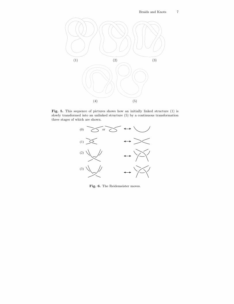
Fig. 6. The Reidemeister moves.
8 Patrick D. Bangert
who thought that knotted vortex tubes in the luminiferous ether would makea good model for the elusive atomic theory. This physical application wasabandoned when it became clear the the ether did not exist through theMichelson-Morley experiment in 1887. In spite of this, the mathematics washere to stay. Tait first published his work in 1877 at which time he was ableto present a long list of knots. It was his purpose to construct the list in orderof increasing number of crossings in the knot.
(a) (b)
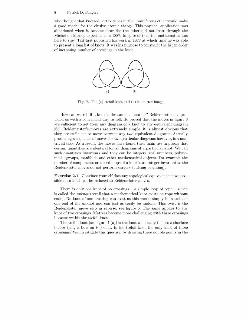
Fig. 7. The (a) trefoil knot and (b) its mirror image.
How can we tell if a knot is the same as another? Reidemeister has pro-vided us with a convenient way to tell. He proved that the moves in figure 6are sufficient to get from any diagram of a knot to any equivalent diagram[65]. Reidemeister’s moves are extremely simple, it is almost obvious thatthey are sufficient to move between any two equivalent diagrams. Actuallyproducing a sequence of moves for two particular diagrams however, is a non-trivial task. As a result, the moves have found their main use in proofs thatcertain quantities are identical for all diagrams of a particular knot. We callsuch quantities invariants and they can be integers, real numbers, polyno-mials, groups, manifolds and other mathematical objects. For example thenumber of components or closed loops of a knot is an integer invariant as theReidemeister moves do not perform surgery (cutting or gluing).
Exercise 2.1. Convince yourself that any topological equivalence move pos-sible on a knot can be reduced to Reidemeister moves.
There is only one knot of no crossings – a simple loop of rope – whichis called the unknot (recall that a mathematical knot exists on rope withoutends). No knot of one crossing can exist as this would simply be a twist ofone end of the unknot and can just as easily be undone. This twist is theReidemeister move zero in reverse, see figure 6. The same applies to anyknot of two crossings. Matters become more challenging with three crossingsbecause we hit the trefoil knot.
The trefoil knot (see figure 7 (a)) is the knot we usually tie into a shoelacebefore tying a bow on top of it. Is the trefoil knot the only knot of threecrossings? We investigate this question by drawing three double points in the

Braids and Knots 9
plane (do not differentiate between over and undercrossings yet) which arethe intersections of two short line segments each. Then connect the endpointsof the line segments in all possible ways without causing further crossings inthe plane. You will find that all of these will unravel to give the unknotby Reidemeister moves of type zero except the trefoil knot. The trefoil knotcomes in two natural flavours: the standard type (figure 7 (a)) and the mirrorimage of the standard type (figure 7 (b)). The mirror image of a knot isobtained by switching all of its crossings (see figure 7 (b)). This method isessentially the one which Rev. Kirkman used in the 19th century to constructa list of all knots up to and including ten crossings. The labour involved inthis task is prodigious. To complete the list of all knots of three crossings wemust ask:
31 41
51 52
61 62
63
Fig. 8. The prime knots with fewer than seven crossings and their names fromstandard tables. The knot 31 is the trefoil knot of figure 7 (a).
Exercise 2.2. Is the trefoil equivalent to its mirror image? [Hint: This meansthat you have to find a continuous deformation of the trefoil into its mirrorimage if they are equivalent or a proof that it is not possible otherwise. The
10 Patrick D. Bangert
typical method is to look for an invariant if you suspect that they are notequivalent. If you can show that the value of the invariant is different for thetwo knots, then you have shown that they are different.]
The answer to exercise 2.2 is that the trefoil is not equivalent to its mirrorimage. This is shown by computing an invariant quantity called Alexanderpolynomial for both knots. We will compute the polynomials for both trefoilsin section 2.5.
We will motivate the result here by computing a quantity called writhewhich is an invariant of all the Reidemeister moves except the zeroth one.Imagine you want to hang a painting on the wall and you are putting a screwinto the wall to hold the painting up. You twist the screw clockwise to get itinto the wall and counterclockwise when you’ve made a mistake and wish toget it out again. We consider progress positive and mistakes negative so thata crossing in a knot which is achieved by a clockwise rotation of the handsas they follow the orientation of the knot is assigned a weighting of +1; theopposite kind is assigned a weight of −1. The writhe w of a knot is the sumof the weights over all the crossings. Let us pick the orientation in which thetopmost arch on the trefoils in figure 7 points to the left. Then the standardtrefoil has w = 3 and the mirror image w = −3.
Exercise 2.3. Prove that writhe is invariant for all Reidemeister moves ex-cept move zero.
Using such methods, it is possible to construct a large table of knots.In figure 8 we show the first seven knots after the unknot. It is understoodthat the two ends of the rope must be joined to yield the mathematicalknot. We present them in this fashion for ease of understanding and practicalexperimentation.
The question is: Can we find a general method to determine equalityor otherwise for any two knots? The answer is yes, but with qualifications.There exists a method due to Waldhausen, Hakken, Hemion and others butit is so inefficient that it is not possible to use for knots for which we do notknow the answer already [39]. There exists a theorem due to Alexander whichstates that every knot can be represented by a braid [4] which we prove intheorem 2.9. This gave the motivation for people to study braids in orderto try to help classify knots. The greatest thrust came from Markov whoproved a result for braids similar to Reidemeister move result for knots [55].Using Markov’s theorem to classify knots has proven difficult however andthe search continues.
Braids have proven tremendously useful in spite of the fact that they havenot lead to a complete knot classification scheme. Many invariant of knotsare naturally defined on braids. The most revolutionary invariant, the Jonespolynomial, was discovered using braid theory. Beyond this, braids have manyapplications to various fields as we shall discover in the sections to come.

Braids and Knots 11
An operation to combine knots can be defined which we are going to callknot addition and denote it by #.
Definition 2.4. Given two knots K and L, we define the knot sum K#L asthe knot obtained by cutting both K and L at a random location and gluingthem together with respect to their orientations.
This is a simple operation but it is not at all obvious that it is well defined.One can show that: (1) The sum is independent of the points on K and Lchosen as cutting points [60], (2) any knot can be uniquely factorized into afinite length sum of knots [67], (3) this sum may actually be determined [68].Property (1) makes the concept well-defined. The second property establishesthe existence of prime knots, i.e. knots that may not be decomposed into thesum of others and also that classifying prime knots will classify all knots.The third property means that this is, at least in theory, possible to actuallycompute. However, the algorithm to find the unique decomposition is thealgorithm alluded to previously and thus this is not a practical method. Itcan be shown that there does not, in general, exist an inverse to the operationof addition of knots. As one may show that knot addition is associative, knotsform a semi-group but not a group under the operation of addition [60].
2.3 The Topological Braid
l a a a1 1 2 3
l b b b2 1 2 3
A
B
C
A
B
C
(a) (b)
Fig. 9. (a) An example of the definition of a topological braid (see definition 2.5)and (b) an elementary deformation as defined in definition 2.6.
We know from section 1 what a braid is. Mathematically, we have to beslightly more careful.
Definition 2.5 (n-braid). Let l1 and l2 be two parallel lines in a planeP and let A = {a1, a2, · · · , an} and B = {b1, b2, · · · , bn} be sets of pointson l1 and l2 respectively. An n-braid is a set of (possibly oriented) n non-intersecting polygonal curves which have exactly one endpoint in A and onein B such that all points in A or B are the endpoints of exactly one of thesecurves and such that any line l parallel to l1 and l2 crosses any curve in atmost one point.

12 Patrick D. Bangert
An example of a 3-braid, in which we have labelled the lines l1 and l2 aswell as the point sets A and B, is shown in figure 9 (a); note that the plane Pis understood to be the plane of the paper. In this example, we have 3 curveseach of which have two endpoints, one in A and one in B. These curves gofrom l1 to l2 monotonically, they do not double back on themselves. This isthe meaning that no line parallel to l1 and l2 may cross any curve in morethan one point. In fact it is this requirement that makes braids substantiallysimpler than knots and allows a group structure to be defined on braids. Ann-braid in the form of definition 2.5 is also called an open braid. We shalldrop the n from n-braid when no confusion can arise.
The normal braid which is braided into peoples’ hair fulfills these require-ments. One end of all the strings is fixed on the person’s head and others areheld in place by some form of rubber band. The braiding in the middle is donein a way that each bundle of hairs goes from top to bottom monotonically.Some Celtic designs used as borders in the Book of Kells or other illuminatedbooks or more commonly used as trimmings for medieval clothing, necklaces,pendants and belts are not usually braids conforming to this definition astheir strings often return to a point close to their origin and thus contain alocal maximum or minimum.
Whenever we define a new mathematical object, we desire an equivalencerelation for the possible instances of this object. As braid theory is a topo-logical pursuit, we will allow ourselves the usual freedom of topology whichmeans that we will allow the object to be distorted in any way as long as thiscan be done continuously. So we may bend, stretch and pull a string but wemay never cut a string or glue two strings together; such actions are calledsurgery and are said to change the topology. For braids, it is clear that ifwe do not fix the endpoints of the curves, we shall be able to transform anybraid into any other yielding a rather boring theory; thus we also require theends to be fixed. We will call the equivalence relation for braids under theseconditions isotopy. Before we can define isotopy, we must define what wemean by a topological deformation. An elementary deformation is the basisfor all topological deformations.
Definition 2.6 (elementary deformation). Suppose that a braid string(recall that it was defined as a polygonal curve) has points A and B as vertices.We may then create a further point C, delete the segment AB and createthe segments AC and CB. This deformation, and its inverse, is called anelementary deformation if and only if the triangle ABC does not intersectany other strings and only meets the current string along its side AB. Seefigure 9 (b) for an illustration.
Definition 2.7 (braid isotopy). Two braids α and β are called isotopic,denoted α ≈ β, if and only if α can be transformed into β using a finitenumber of elementary deformations.

Braids and Knots 13
Suppose we were to label the string which intersects the point bi by i. Onl2, the string labels from left to right would thus be in numerical order whereason l1 they may not be ordered numerically. If we list the numerical labels ofthe strings which intersect l1 from left to right, we obtain a permutationon the set of integers {1, 2, · · · , n}. A braid thus induces a permutation onthe set of the first n integers. For example, the braid in figure 9 induces thepermutation [2, 3, 1]. The fact that the induced permutation is an equivalenceclass invariant follows immediately from the requirement that the endpointsbe fixed.
a a a1 2 3
b b b1 2 3
Fig. 10. The braid from figure 9 is closed here. It is immediate upon simple trans-formation that this knot is the same as the simple loop or the unknot.
An open braid may be closed to yield a knot. See figure 10 for the closureof the braid from figure 9. A closed braid, denoted α, is obtained from anopen n-braid α by deleting l1 and l2 and connecting points ai and bi withnon-intersecting polygonal curves in P for all i : 1 ≤ i ≤ n. It is clear thatthe closure of any braid yields a knot. Thus some knots may be representedas closed braids. Unfortunately determining the closed braid, given a knot, isnot so easy. It is however possible and we shall solve this problem in sections3.4 and 3.5. The proof of the fact that all knots may be represented as closedbraids, Alexander’s theorem, gave the initial momentum for studying braidsin detail [4]. Artin took up the challenge and constructed a theory of braidswith a view to use them to deal with knots.
Exercise 2.8. A simple knot invariant is the number of components a knothas. Show that the number of components of the knot α is equal to thenumber of cycles in the permutation that the braid α induces.
Alexander’s theorem is usually proved by giving a topological methodwith which to deform a knot into a closed braid. There exist several distinctmethods of doing so but most are not suitable for use; they are only employed

14 Patrick D. Bangert
to establish the theorem. The proof given here is fundamentally different andnew to the best knowledge of the author. The theorem assumes that the knotis oriented but if not the transformation is accurate up to orientation change.
Theorem 2.9 (Alexander [4]). Every knot may be represented as a closedbraid.
Proof. Consider an oriented straight line a in R3 which we will call the axis.
Choose a point O on a and construct a cylindrical polar coordinate systemwhich has O as its origin. The positive z, or upward vertical, direction isdirected parallel to a in the direction of its orientation. The polar angle φincreases in the counterclockwise direction, as usual. Using this system, thetheorem claims that every knot K can be deformed with respect to a insuch a way that the polar angle of a point P going along any componentof K strictly increases or more simply: As we travel along the knot we willgo around the axis a without ever changing our counterclockwise direction.Suppose we have n straight line segments si for 1 ≤ i ≤ n with endpointsRi and Si such that the polar angle of Si, φ(Si) is is larger than φ(Ri).We may form any knot by subdividing these segments into a finite numberof straight subsegments, moving the endpoints of the subsegments and per-forming surgery which identifies Ri and Si for all i. Here, we will form theknot K by keeping Ri fixed and moving the point Si creating new points Qi,j
indexed by j as necessary. Whenever it becomes necessary to move Si to aposition of lower polar angle than the last Qi,j created, move Si once arounda creating a suitable number of points doing so and then continuing. Afterthe required knot is formed, we perform the surgery of identifying Ri and Si.By definition of a knot as a polygonal curve such a construction is alwayspossible.
An example of this method applied to forming the trefoil knot is given infigure 11. This proves the theorem. ��
2.4 The Braid Group
We note that any braid can be represented by a vertical stack of two typesof crossing, see figure 12. When all strings are vertical apart from strings iand i + 1, we will denote this crossing by σi or σ−1
i depending on whetherstring i overcrosses or undercrosses string i + 1 respectively. It is thus clearthat any braid can be specified by a string of these symbols. We agree tothe convention that the left to right direction of the symbols representinga braid shall correspond to the upward direction of the braid; that is, thelowest crossing corresponds to the first symbol. This is a convention andsome other authors use the opposite convention. While care is required, noserious consequences arise from this choice. For example, the braid in figure2 (b) is σ5
1 (the power means that the symbol σ1 was repeated five times)and the braid in figure 4 is
(σ1σ
−12 σ−1
1 σ2
)3. From now on, we shall denote a
braid by these symbols.

Braids and Knots 15
z
fO
R S
O
R
Q1
Q2
SO
(a) (b) (c)
R
Q1
Q2
Q3
Q4
Q5
Q6
Q7Q8Q9
Q10
Q11
Q12
Q13
Q14
S
Fig. 11. Constructing the trefoil knot as a closed braid, see proof of theorem 2.9for a discussion.
Fig. 12. The generator σi and its inverse σ−1i for the braid group Bn.
Definition 2.10 (braid word). We will call any sequence of σ±1i a braid
word.
Definition 2.11 (positive and negative braid word). If a braid wordcontains only σi (and no σ−1
i ) then it will be called positive. However, if itis contains only σ−1
i (and no σi) then it will be called negative.
Consider the braid σ3σ1 displayed in figure 13 (1a). This braid is clearlytopological equivalent to the braid σ1σ3 displayed in figure 13 (1b). Moregenerally, every time two neighboring crossings are on distinct pairs of strings,the order in which these crossings are listed in the braid word does nottopologically matter. Thus we arrive at the rule that
σiσj ≈ σjσi for |i− j| > 1 (1)

16 Patrick D. Bangert
5cm
(a) (b) (a) (b)
(1) (2)
Fig. 13. (1) Two non-interfering crossings can be listed in either order and (2) acrossing may be moved underneath an arch which overcrosses both strings involved
which is usually called the far commutation relation as it embodies the factthat generators sufficiently far from each other commute.
It also becomes clear that if we have an arch which over or undercrossestwo strings which then cross (see figure 13 (2a)), this crossing may be movedonto the other side of the arch (see figure 13 (2b)). Thus the braids σ1σ2σ1
and σ2σ1σ2 are topologically equivalent. As this can hold anywhere in a braid,we arrive at the second rule that
σiσi+1σi ≈ σi+1σiσi+1 (2)
which is typically called the braid relation. We find this name too vague andso we will refer to this relation as the bridge relation as it symbolizes thatanything not in conflict with the principal pillars may move freely both belowand above a bridge.
After some experimentation, one notices that all the moves one may makeon a braid while preserving its topology can be reduced to applying the rulesin equations 1 and 2 to the braid word. We would like to prove that this isalways so.
Theorem 2.12. (Artin [6] [7]) The equivalence relation upon braid wordsdefined by the relations 1 and 2 is identical to the equivalence relation ofbraid isotopy (see definition 2.7) upon the braids represented by the braidwords.
Proof. Recall that any knot may be represented as a closed braid. The braidcontains all the crossings and Reidemeister’s moves define equivalence ofknots. Thus braid equivalence is Reidemeister equivalence of the braid. Movezero would create an object which is not a braid but the others apply. Trans-lating these into the σi notation and simplifying yields the given presentation.

Braids and Knots 17
From figure 12, it is clear that σ−1i is the inverse of σi. As we represent a
braid by a braid word in the σi from the bottom up, we can easily concatenatetwo braids together. The braid αβ is constructed from the braids α and β byidentifying the top ends of α with the bottom ends of β. It is obvious thatconcatenation is associative, i.e. (αβ)γ ≈ α(βγ) and that the concatenationof two braids is a braid. Suppose ι is the braid of n vertical strings and nocrossings. We have ια ≈ αι ≈ α for any n-braid α. The braid ι acts as anidentity. Since we have closure, associativity, inverses and an identity, the setof n-braids forms a group generated by the generators σi. We will denote thisgroup by Bn and refer to this family of groups as the braid groups. Becauseof theorem 2.12, Bn has the presentation
Bn =⟨{σ1, σ2, · · · , σn−1} : σiσi+1σi ≈ σi+1σiσi+1,
σiσj ≈ σjσi for |i− j| > 1
⟩(3)
It is instructive to consider the braid group from another point of viewwhich curiously leads to the same presentation as given above in equation3. Consider the space between the two parallel planes which contain l1 andl2 respectively after the braid has been removed from it. This space has afundamental group which may be represented by a series of loops beginningand ending on some randomly chosen base point b and going around theremoved braid strings. There are n distinct such loops which we shall call xi
with i running from 1 to n. The fundamental group is free of rank n withthe xi as generators. x1 is the loop around the first string from the left oneach level and so on for the other xi. From level to level a reassignmentof generators becomes necessary. This is called an automorphism and theparticular one we need here, ai is defined by
ai : xi → xi+1; xi+1 → x−1i+1xixi+1; xp → xp (p �= i, i + 1) (4)
The map α : σi → ai is a homomorphism of Bn into the automorphismgroup of Fn, the free group of rank n. It can be shown that the ai generatea group with presentation identical to equation 3 under the homomorphismα. In other words, a braid word may be regarded as an automorphism of Fn.As the mapping merely consists of a change of symbol for the generators, itis frequently useful not to make a distinction between a braid word as anelement of Bn and as an automorphism of Fn. In the next section, we willintroduce some other presentations of the braid group.
2.5 Other Presentations of the Braid Group
The presentation of Bn given in equation 3 is called the Artin presentation asit was Artin who first used it in the paper which founded the field. The factthat braids admit a group structure simplifies their treatment tremendously.It can be shown that knots do not admit a group structure and this is onereason why the problem of deciding if two knots are equal is so different from

18 Patrick D. Bangert
the similar question about braids. It is difficult, however to extract usefulinformation from a presentation of a group. For this reason it is useful tosearch for other presentations of the same group with special properties.
The Artin presentation has the appeal that it is very topological. It is easyto draw the braid given the braid word and it is easy to read off the braidword from a braid. Furthermore, both the far commutation and the bridgerelations are simple to perform. One disadvantage is that each braid grouphas a different number of generators. Consider putting a = σ1σ2 · · ·σn−1 andσ = σ1. After some manipulation, we find the presentation
Bn =⟨{a, σ} : an ≈ (aσ)n−1, σa−jσaj ≈ a−jσajσ for 2 ≤ j ≤ n
2
⟩(5)
which we call the Coxeter presentation. The Coxeter presentation has theadvantage that all braid groups have just two generators but we have lostsome of the topological correspondence.
It would be nice to have a matrix representation of the braid groups. Tothis end, we will represent the identity matrix of n rows and columns byIn (recall that the identity matrix has unity entries in the leading diagonaland zeros everywhere else). Then we define the mapping φn(σi) of an Artingenerator σi to a matrix of n rows and n columns whose entries are Laurentpolynomials in the variable t (Laurent polynomials allow both positive andnegative powers of the variable). Expressed formally, this means
φn : Bn → GL(n,Z
[t±1
])(6)
where Z is the ring of polynomials. The mapping is defined by
φn(σi) =
⎛⎜⎜⎝
Ii−1 0 0 00 1− t t 00 1 0 00 0 0 In−i−1
⎞⎟⎟⎠ (7)
It can easily be shown that φn is a homomorphism, i.e. that φn(σiσj) =φn(σi)φn(σj) where multiplication in GL
(n,Z
[t±1
])is the usual matrix mul-
tiplication. A representation is termed faithful when the mapping φ givingrise to it is injective, i.e. when x �= y implies φ(x) �= φ(y). This representa-tion is faithful for n ≤ 3 [54] and not for n ≥ 5 [13]. For n = 4 the answer isunknown.
It should now be easy to write down a matrix representation for any braidword. For example, if n = 3, then for φn(σ1σ2) we have
φn(σ1)φn(σ2) =
⎛⎝ 1− t t 0
1 0 00 0 1
⎞⎠⎛⎝1 0 0
0 1− t t0 1 0
⎞⎠ =
⎛⎝1− t t− t2 t2
1 0 00 1 0
⎞⎠ (8)
This representation is called the Burau representation.
Braids and Knots 19
Recently a new presentation was invented by Birman, Ko and Lee [15]which they used to solve the word and conjugacy problem in a new way. Thegenerators akl are defined by
akl = (σk−1σk−2 · · ·σl+1)σl
(σ−1
l+1σ−1l+2 · · ·σ−1
k−1
)(9)
Topologically this is a crossing between two arbitrary braid strings k and l.In akl, string k overcrosses string l and both strings overcross all other stringin between them to be able to cross and then overcross the in between stringsagain to return to their original (but now switched) positions. Using thesegenerators, Bn has the presentation
Bn =
⟨{ats; n ≥ t > s ≥ 1} :
atsasr = atrats = asratr,atsarq = arqats for(t− r)(t − q)(s− r)(s − q) > 0
⟩(10)
which we call the band-generator presentation. In the Artin representation,we number the strings from left to right on each level. Suppose we were tolabel each string with a unique label which it would carry throughout thebraid. At the bottom of the braid, we number the strings from one to n as wego from left to right. Each crossing in which string i overcrosses string j islabelled with the generator gij . This presentation is called the colored braidpresentation as the string labels act like each string was made of a separatecolor. This representation retains the complete information of the braid butit is not immediately apparent whether a crossing is positive or negative inthe Artin sense. Note that this feature means that the generators gij are selfinverse, g2
ij ≈ e the identity. We easily write down the braid group relationsin this presentation to get
Bn =
⟨{gij} for 1 ≤ i, j ≤ n
i �= j:
gijgikgjk = gjkgikgij ,gijgkl = gklgij for(i− k)(i− l)(j − k)(j − l) > 0
⟩(11)
We note that in the colored braid presentation, the fundamental braid Δn
takes the form
Δn = g12g13 · · · g1ng23g24 · · · gn−1 n (12)
=n−1∏i=1
n∏j=i+1
gij (13)
2.6 The Alexander and Jones Polynomials
The Burau representation of the braid group is important in the definitionof a revolutionary knot-invariant called the Alexander polynomial. We beginwith a braid word α, construct its Burau representation φn(α) and take the

20 Patrick D. Bangert
determinant of the matrix [φn(α)− In]1,1 where the subscript indicates thatthe first row and column should be deleted. This determinant can be shownto be a topological invariant of the closure of the braid α and is denoted byα such that
α(t) = det[φn(α) − In]1,1 (14)
Thus the Alexander polynomial of the braid σ1σ2 of the above example is = 1 which happens to be the same value as the Alexander polynomialfor the unknot. While σ1σ2 is actually isotopic to the unknot, we could notconclude this from its Alexander polynomial. The Alexander polynomial isan incomplete invariant in that we can only say that if K �= K′ , thenK �= K ′. The converse is not true, in general. Nevertheless, the Alexanderpolynomial is very important in knot theory. Let us compute the Alexanderpolynomial for both trefoils (see figure 7). The ordinary trefoil is the closureof σ3
1 and its mirror is the closure of σ−31 . Now we have
φ2
(σ3
1
)=(
(1− t)3 00 t3
)φ2
(σ−3
1
)=(
(1− t)−3 00 t−3
)(15)
and thus
σ31
= t3 − 1 σ31
= t−3 − 1 (16)
And since the Alexander polynomials of the two trefoils are distinct, the knotsmust be distinct.
Many other polynomials invariants have been devised after the Alexanderpolynomial, the most important is the Jones polynomial. The Jones polyno-mial is also an incomplete invariant of knots which was originally constructedin terms of braids. We shall not prove that it is an invariant, nor that it isincomplete but we shall give an easy method to obtain it. Even though it isincomplete, it is a very powerful invariant in that it distinguishes many knotsnot distinguished by other invariants such as the Alexander polynomial.
We define the tensor product of a p× q matrix A and a r× s matrix B by
A⊗B =
⎛⎜⎜⎜⎝
a11B a12B · · · a1qBa21B a22B · · · a2qB
......
. . ....
ap1B ap2B · · · apqB
⎞⎟⎟⎟⎠ (17)
A⊗B is clearly a pr× qs matrix. We also define the trace of a n× n matrixC by
tr(C) =n∑
i=1
cii (18)
Consider the matrix
μ(t) =(
1 00 t
)(19)
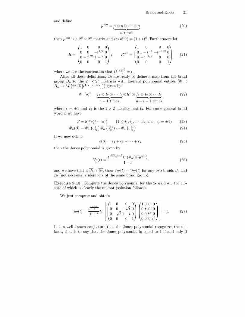
Braids and Knots 21
and defineμ⊗n = μ⊗ μ⊗ · · · ⊗ μ︸ ︷︷ ︸
n times
(20)
then μ⊗n is a 2n × 2n matrix and tr (μ⊗n) = (1 + t)n. Furthermore let
R =
⎛⎜⎜⎝
1 0 0 00 0 −t1/2 00 −t1/2 1− t 00 0 0 1
⎞⎟⎟⎠ ; R−1 =
⎛⎜⎜⎝
1 0 0 00 1− t−1 −t−1/2 00 −t−1/2 0 00 0 0 1
⎞⎟⎟⎠ (21)
where we use the convention that(t1/2
)2= t.
After all these definitions, we are ready to define a map from the braidgroup Bn to the 2n × 2n matrices with Laurent polynomial entries (Φn :Bn →M
(2n, Z
[t1/2, t−1/2
])) given by
Φn (σεi ) = I2 ⊗ I2 ⊗ · · · I2︸ ︷︷ ︸
i− 1 times
⊗Rε ⊗ I2 ⊗ I2 ⊗ · · · I2︸ ︷︷ ︸n− i− 1 times
(22)
where ε = ±1 and I2 is the 2 × 2 identity matrix. For some general braidword β we have
β = σε1i1
σε2i2· · ·σεk
ik(1 ≤ i1, i2, · · · , in < n; εj = ±1) (23)
Φn(β) = Φn
(σε1
i1
)Φn
(σε2
i2
) · · ·Φn
(σεk
ik
)(24)
If we now defineε(β) = ε1 + ε2 + · · ·+ εk (25)
then the Jones polynomial is given by
Vβ(t) =t
ε(β)−n+12 tr (Φn(β)μ⊗n)
1 + t(26)
and we have that if β1 ≈ β2, then Vβ1(t) = Vβ2
(t) for any two braids β1 andβ2 (not necessarily members of the same braid group).
Exercise 2.13. Compute the Jones polynomial for the 2-braid σ1, the clo-sure of which is clearly the unknot (solution follows).
We just compute and obtain
Vσ1(t) =t
1−2+12
1 + ttr
⎡⎢⎢⎣⎛⎜⎜⎝
1 0 0 00 0 −√t 00 −√t 1− t 00 0 0 1
⎞⎟⎟⎠⎛⎜⎜⎝
1 0 0 00 t 0 00 0 t2 00 0 0 t3
⎞⎟⎟⎠⎤⎥⎥⎦ = 1 (27)
It is a well-known conjecture that the Jones polynomial recognizes the un-knot, that is to say that the Jones polynomial is equal to 1 if and only if
22 Patrick D. Bangert
the knot is isotopic to the unknot. Many people have been searching for aproof and a counterexample and none has been found thus far. Resolving thisquestion is one of the more important open problems in knot theory.
Proving that the Jones polynomials is an invariant of closures of braids iseasy. For reasons of space, we simply outline the equations that need to bechecked by straightforward calculations.
Theorem 2.14. The Jones polynomial is a knot invariant.
Proof. By direct calculation, check
1. The mapping Φn is a homomorphism from Bn to M(2n, Z
[t1/2, t−1/2
]).
This can be done by checking that
Φn (σiσj) = Φn (σjσi) ; Φn (σiσi+1σi) = Φn (σi+1σiσi+1) (|i−j| > 1)(28)
2. By Markov’s theorem, two closed braids are isotopic if and only if theycan be reached from each other by conjugacy and stabilization. Thus weneed to check if the Jones polynomial is invariant under these two moves,
Vγβγ−1(t) = Vβ(t); Vβ(t) = Vβσ±1
n(t) (γ, β ∈ Bn) (29)
The polynomial invariants can be calculated using so-called skein rela-tions. These relations are expressions relating the polynomials of knots thatare identical except for a single local change. In braid language, the Alexanderpolynomial of the closed braid β ∈ Bn, Aβ(z) is given by the relation
Aβσi(z)−Aβσ−1i
(z) = zAβ(z) (30)
together with the boundary condition that if the closure of β is the unknot,A(z) = 1. The Jones polynomial Jβ(z) has the same boundary condition buttakes the skein relation
Jβσi(z)z
− tJβσ−1i
(z) =(√
z − 1√t
)Jβ(z) (31)
Using these skein relations, it is possible to calculate the polynomial invari-ants straight from the diagram by successively eliminating crossings [48].
2.7 Properties of the Braid Group
In this section we will prove various propositions which enumerate the basicproperties of braids. The Artin presentation will be used for all these as formost of the rest of the chapter.
Recall that the center of a group is the set of all those elements whichcommute with all other elements in that group. The centre of the braid groupswill become important in many places and so we will construct it.
Braids and Knots 23
Definition 2.15 (fundamental word). The fundamental braid word Δn ∈Bn is defined by
Δn = σ1σ2 · · ·σn−1σ1σ2 · · ·σn−2 · · ·σ1σ2σ1 (32)
It is a simple matter of applying the braid group relations to find that
Δ2n = (σ1σ2 · · ·σn−1)
n (33)
Proposition 2.16. The center C(Bn) of the braid group Bn is the set
C(Bn) ={Δ2i
n
}(34)
for any (positive, negative or zero) integer i.
Definition 2.17. The ascending braid word aj is defined by aj = σ1σ2 · · ·σj.
Proposition 2.18. In Bn, we have σiaj ≈ ajσi−1 for 1 < i ≤ j < n.
Proposition 2.19. For all i we have σiΔn ≈ Δnσn−i.
Definition 2.20. Two positive n-braid words a and b are called positivelyequal if and only if there exists a sequence of words Wi with 0 ≤ i ≤ p forsome finite p for which W0 = a, Wp = b, Wi is obtained from Wi−1 by a singleapplication of one of the defining relations of Bn, and all Wi are positive.
In other words, two braids are positively equal if we can transform oneinto the other without ever having to use an inverse generator.
Proposition 2.21. Two equal positive braid words are positively equal.
2.8 Algorithmic Problems in the Braid Groups
We have defined braids, elucidated their connection with knots and founda group structure on braids. This group structure has certain properties ofwhich we enumerated a few important ones in the last section. There area number of questions which we may readily ask about braids, the mostsignificant of which we shall describe in this section. Clearly, we wish toknow both necessary and sufficient conditions for equivalence.
Definition 2.22 (word problem). Given two braid words α, β ∈ Bn, theword problem asks whether α ≈ β.
The question of whether α ≈ β is identical to the question of whetherαβ−1 ≈ e, the identity in Bn. Thus the word problem reduces to recognizingthe identity element.
Recall that two elements a and b of some group G are called conjugate,denoted a ≈c b, if and only if there exists a c ∈ G such that a ≈ cbc−1.The conjugacy condition becomes αγ ≈ γβ for two braid words α, β ∈ Bn
to be conjugate with respect to a third braid word γ ∈ Bn. We are naturallyinterested under what conditions such a commutation relation exists.

24 Patrick D. Bangert
Definition 2.23 (conjugacy problem). Given two braid words α, β ∈ Bn,the conjugacy problem asks whether there exists a third braid word γ ∈ Bn
such that αγ ≈ γβ.
Suppose α ≈ β, then we also have αγ ≈ γβ for γ ≈ e. Thus any equal braidwords are also conjugate but two conjugate braid words are not necessarilyequal and so the conjugacy problem subsumes the word problem.
The most central question in knot theory is that of classification: Giventwo knots K1, K2 are they topologically equivalent K1 ≈ K2? Markov hasfound it possible to translate this question into a question about braids.Imagine closing the braid cbc−1. We may move the subbraid c through theclosure part so that it emerges on top of the rest of the braid, i.e. becomesbc−1c ≈ b. In other words, conjugation of a braid preserves closed braidisotopy: Any two conjugate braids represent equivalent knots. Conjugationis a sufficient condition but unfortunately not necessary. The braid e ∈ B1
is just a single vertical line segment which closes to the unknot. The braidσ1 ∈ B2 is the braid of single positive crossings which also closes to theunknot. As the braids are in different braid groups, they have a differentnumber of strings and are thus not conjugate to each other. Such braids canbe related through a move called stabilization.
Definition 2.24 (stabilization move). Given a braid α ∈ Bn, the op-eration α ↔ ασ±1
n is called stabilizing the braid and is referred to as thestabilization move.
Note that stabilization changes the number of strings in the braid by oneand that we refer to both the addition and removal of a string as stabilizing.Starting with e ∈ B1, we stabilize once to obtain σ1 ∈ B2. In this way, we canmove between two braids in different braid groups. Markov’s theorem statesthat conjugacy and stabilization are enough for knot equivalence.
Theorem 2.25 (Markov [55], Birman [14]). Given two braids α ∈ Bn
and β ∈ Bm, we have α ≈ β if and only if β may be obtained from α by afinite sequence of conjugacy or stabilization moves; we denote this by α ≈M βand call α and β Markov equivalent.
In [55], Markov stated this theorem but the first complete published proofappeared in [14]. We shall not prove this theorem here as it is difficult andlengthy and would distract from the flow of the chapter. It is clear that weare interested in approaching knot classification from a braid theory point ofview.
Definition 2.26 (Markov problem). Given two braid words α ∈ Bn andβ ∈ Bm, the Markov problem or algebraic link problem asks whether α ≈M
β.

Braids and Knots 25
By Markov’s theorem, a solution to the Markov problem would providea solution to the knot classification problem. As the Markov problem sub-sumes the conjugacy problem, we are presented with a hierarchy of threecombinatorial problems in group theory which would have significant weightif a solution were found. Solutions exist to the word and conjugacy problemsand we shall develop new solutions in later sections. A solution to the Markovproblem only exists in the sense that there exists a knot classification schemebased on 3-manifold classification. This is an indirect and unusable solutionas it is exponential in the amount of computing time required as a functionof the crossing number of the knots concerned.
As many braid words represent the same braid, we are naturally leadto ask for a particularly simple representative. A very natural definition of“simple” in the case of a braid word is the least length possible; the shorterthe word, the simpler it is. As length has an obvious minimum, we formulatethe minimal word problem.
Definition 2.27 (minimal word problem). Given a braid word α ∈ Bn,the minimal word problem asks one to find a braid word αm ∈ Bn such thatαm ≈ α and L(αm) ≤ L(α′) for any braid word α′ ≈ α. The word αm isthe minimal word as it is, by definition, the shortest word in its equivalenceclass.
The word problem is frequently solved by devising an algorithm whichfinds a unique representative for the equivalence class of the element underconsideration. In many groups, this so called normal form is also of mini-mum length in the equivalence class so that word problem and minimal wordproblem are solved together. Examples of such groups include free groups,HNN-extensions and free products. For the braid groups, we shall find thatthe minimum word problem is far more complicated to solve than the wordproblem. In fact, under some very reasonable assumptions, the minimumword problem in the braid groups can only be solved by what amounts toa global search of the equivalence class. We shall outline these assumptionsand the methods by which the global search may be done in later sections.
3 Braids and Knots
3.1 Notation for knots
Dowker-Thistlethwaite Code When he originally invented knot theory,Tait sought to construct a table of distinct prime knots. Two tasks had to beundertaken: (1) An exhaustive list of all possible knots had to be constructedand (2) all duplicates had to be struck from that list. Tait used mainly com-binatorial methods to construct an exhaustive list and then tried to eliminateduplicates by trying to deform knots into each other. Tait labelled each cross-ing by a letter of the alphabet. He named a knot by starting at some random

26 Patrick D. Bangert
Start
1 4 2 5
6 3
Fig. 14. The procedure for obtaining the Dowker-Thistlethwaite code for the trefoil.
point and going along it in the direction of its orientation, writing down thelabel of the crossings as he passed them. This string of letters is called theTait code of a knot. Clearly a knot with n crossings has a name consisting of2n letters. There exist a finite, though large, number of possible such namesfor any n. Not all possible names can arise from naming a knot, however andTait was able to find methods to determine if a specific name was valid.
Dowker and Thistlethwaite improved Tait’s methods and introduced theirown naming convention [35]. Consider a knot of n crossings and start at arandom point going along the knot in the order of its orientation. Namethe crossings in numerical order as you pass them giving each crossing twonumerical labels (you will pass each crossing twice before returning to thestaring point). Each crossing will have two numbers associated with it, i andj, say. We can construct an involution a from these by putting a(i) = j anda(j) = i. Thus we have a(a(k)) = k for any label k. Note that a reversesparity, that is if i is odd and a(i) = j, then j is even and vice-versa. Weagree to write ai for a(i), S for the sequence a1, a2, · · · , a2n and Sodd for thesequence a1, a3, · · · , a2n−1. The sequence Sodd completely determines both Sand a [35].
There are 2n different possible starting points on the knot and if it hasno orientation, there are two possible orientations. Not all sequences Sodd areidentical. The standard sequence Sstd for a knot will be the lexicographicalminimum over all possible Sodd. Consider, for example, the trefoil knot infigure 14. The starting point is labelled in the figure and we proceed to namethe three crossings twice each in the order in which we encounter them. Thisgives rise to the involution
a1 = 4, a2 = 5, a3 = 6, a4 = 1, a5 = 2, a6 = 3 (35)
which results in Sstd = 4, 6, 2.Dowker and Thistlethwaite were able to determine both necessary and
sufficient conditions for a sequence of number to be realizable as a knot. Thisalgorithm is relatively simple and quick to implement and has been used

Braids and Knots 27
by them to tabulate knots. This code is very compact and easy to obtainfrom a knot, but their tabulation methods focus on enumerating all possiblesequences and so we ask: How may we recover the knot given the code?
We note first of all that a knot of n crossings will get 2n labels (2n beingnecessarily even). Suppose Sstd = b1, b2, · · · , bn and the original involution isa. As Sstd is a standard sequence, we have that a2i−1 = bi for i ranging fromone to n. Because of the definition of a, we then have
a(a(2i− 1)) = a(bi) = 2i− 1 (36)
Since a reverses parity and we list only the ai for i odd in the standardsequence, all these ai are even. Thus we have recovered the entire involutiona. The crossings of the knot thus get the double names i and bi for i rangingfrom one to n. Having gotten the complete labelling information, we candraw the crossings on our paper as double points and connect them in orderof the labelling and thus retrieve the knot. We may not get the same numberof crossings that we had in the original projection but this does not mattertopologically.
•
•
•
•
0
•
•
•
•∞
•
•
•
•
1
•
•
•
•
−1
Fig. 15. The four elementary tangles.
Conway’s Basic Polyhedra We constructed the Alexander polynomial insection 2.5. Starting from a knot, we must first construct a closed braid iso-topic to the knot, then write down its Bureau representation and take itsdeterminant to obtain the Alexander polynomial. In practise this process,particularly constructing a closed braid representative, is very complicatedand time-consuming. When Conway looked for a mechanizable method, hewas lead to construct a new notation for knots. From this notation, he wasable to extract the Alexander polynomial so straightforwardly that he pro-ceeded to calculate them all by hand rather than mechanize the method.
A knot diagram has crossings and arcs connecting the crossings. If wewere to draw small circles around the crossings and then ignore what is in thecircles, we would have a template for the knot. Into the circles we could insertany of the four elementary tangles of figure 15 to generate several knots, oneof which would be the original knot. The numerical names of the elementarytangles arise from their classification which will not concern us here. Conway’snotation derived from the observation that many knot diagrams are the sameafter the crossings have been so removed. In such a way, we may generatea large number of different knots starting from one such knot template and
28 Patrick D. Bangert
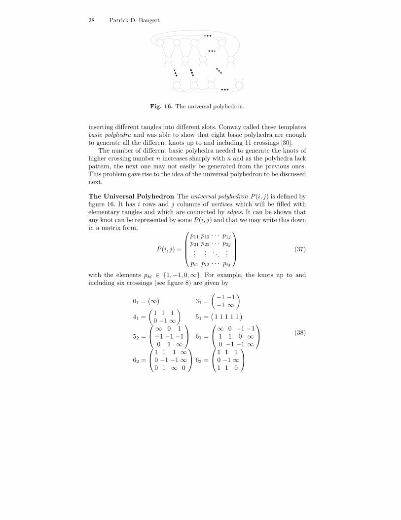
Fig. 16. The universal polyhedron.
inserting different tangles into different slots. Conway called these templatesbasic polyhedra and was able to show that eight basic polyhedra are enoughto generate all the different knots up to and including 11 crossings [30].
The number of different basic polyhedra needed to generate the knots ofhigher crossing number n increases sharply with n and as the polyhedra lackpattern, the next one may not easily be generated from the previous ones.This problem gave rise to the idea of the universal polyhedron to be discussednext.
The Universal Polyhedron The universal polyhedron P (i, j) is defined byfigure 16. It has i rows and j columns of vertices which will be filled withelementary tangles and which are connected by edges. It can be shown thatany knot can be represented by some P (i, j) and that we may write this downin a matrix form,
P (i, j) =
⎛⎜⎜⎜⎝
p11 p12 · · · p1j
p21 p22 · · · p2j
......
. . ....
pi1 pi2 · · · pij
⎞⎟⎟⎟⎠ (37)
with the elements pkl ∈ {1,−1, 0,∞}. For example, the knots up to andincluding six crossings (see figure 8) are given by
01 = (∞) 31 =(−1 −1−1 ∞
)41 =
(1 1 10 −1∞
)51 =
(1 1 1 1 1
)52 =
⎛⎝∞ 0 1−1 −1 −10 1 ∞
⎞⎠ 61 =
⎛⎝∞ 0 −1 −1
1 1 0 ∞0 −1 −1 ∞
⎞⎠
62 =
⎛⎝1 1 1 ∞
0 −1 −1∞0 1 ∞ 0
⎞⎠ 63 =
⎛⎝1 1 1
0 −1∞1 1 0
⎞⎠
(38)
Braids and Knots 29
Theorem 3.1. Every regular projection of any knot may be represented bythe universal polyhedron P (i, j) for some i and j all the vertices of whichcontain elementary tangles.
Proof. A regular projection of a knot is characterized by a finite number nof double points and 2n arcs which connect the double points in a specificmanner. For sufficiently large i and j, the polyhedron P (i, j) can accommo-date all double points in the form of ±1 tangles and can achieve the desiredconnection of these by placement of 0 and ∞ tangles into it. This is obviousbecause the 0 and ∞ tangles represent horizontal and vertical connectors inthe polyhedron. Because this connection may be achieved without ±1 tan-gles, it is clear that no further components, with the possible exception ofunknots, are created. Thus what remains to be shown is that no unwantedunknots will be created.
There are ij vertices and 2ij edges connecting them in the empty polyhe-dron P (i, j). Eliminating one vertex by a 0 or∞ tangle, eliminates two edges.Apart from the ±1 tangles of which there are n, the final polyhedron will con-tain ij−n tangles of type 0 and∞ which will have eliminated 2(ij−n) edgesfrom the original polyhedron, leaving exactly 2n edges which are needed toconnect the double points. Thus there is no extra edge left over which couldpossibly form an extra component. Therefore any knot may be representedusing the basic polyhedron P (i, j) and elementary tangles.
3.2 Braids to Knots
Suppose we have a braid b given by a braid word and we want to denotethe knot that is isotopic to its closure in the standard notations. The univer-sal polyhedron (figure 16) turned through π radians becomes a closed braidtemplate if every vertex is filled with tangles of the types 1, -1 and 0.
The n-braid b will be specified by a function b(t) = σ±1i which gives the
tth Artin generator of b for 1 ≤ t ≤ c where c is the number of crossings in thebraid. The map ξi will map an Artin generator σ±1
j to the elementary tangles1 and -1 if the exponent of the Artin generator is 1 and -1 respectively andi = j and will map any Artin generator to the elementary tangle 0 otherwise,
ξi (σi) = 1 (39)ξi
(σ−1
i
)= −1 (40)
ξi
(σ±1
j
)= 0 for i �= j (41)
The closed braid b can be contained in the polyhedron P (n − 1, c) withpij = ξi (b(j)) with 1 ≤ i < n and 1 ≤ j ≤ c.
For example, b = σ31 . Then b(i) = σ1 for i = 1, 2, 3 and we get
σ31 =
(1 1 1
)(42)
which correctly represents the trefoil knot. In the next section we will gener-alise this example to an infinite family of knots known as torus knots.
30 Patrick D. Bangert
3.3 Example: The Torus Knots
The torus knots are an infinity family of prime knots which have particularlysimple properties and are frequently used as examples in knot theory texts.The connection between braids and knots is readily illustrated in the case oftorus knots and this is what we shall do below.
Definition 3.2. Given two co-prime (no common factors apart from unity)integers p and q, the torus knot Tp,q is constructed by wrapping a closed curvearound the surface of a torus such that it encircles it p times meridionallyand q times longitudinally (respectively the short and the long way around).
Torus knots are completely characterized by the two integers p and q.They are invertible (isotopic under switching the orientation) and chiral (notisotopic to their mirror image) [?]. The fundamental group of their com-plements is given by π1 (Tp,q) = 〈{a, b} : ap = bq〉 [49] from which we mayrecognize the requirement that p and q be co-prime. It may be shown thatTp,q = Tq,p. The torus knots are among the few knots for which the minimalnumber of crossing-switches required to transform the knot into the unknot,i.e. the unknotting number, is known; it is (p− 1)(q − 1)/2 [1]. They are alsoamong the few knots for which the minimal number of crossings in any pro-jection, i.e. the minimal crossing number is known; it is min[p(q−1), q(p−1)][75].
The simplest example of a torus knot is the trefoil. It is not the unknoteven though Tp,1 for any p would be isotopic to the unknot but p and unityare not coprime. The trefoil knot is T3,2 and the knot 51 is T5,2. In general,the closed p-braid (σp−1σp−2 · · ·σ1)
q is isotopic to the torus knot Tp,q. Thisis easily seen by picturing Tp,q on an actual torus. We cut the torus acrossa random meridian (the short way around) and straighten it into a cylinder.The remainder will be the braid above. Moreover, there exists no closed braidrepresentative of Tp,q with less than p strings so that p is the braid index ofTp,q.
Exercise 3.3. Show that the Alexander polynomial of Tp,q is given by
Tp,q =(1− tpq)(1 − t)(1− tp)(1− tq)
(43)
As we have seen, any torus knot can be represented as the p-braid b =(σp−1σp−2 · · ·σ1)
q. By using the method of the last section, we can representTp,q in the polyhedron P (p− 1, q(p− 1)).
Tp,q =
⎛⎜⎜⎜⎜⎝
1 1 · · · 1· · · · · · · · · · · ·
1 1 · · · 11 1 · · · 1
1 1 · · · 1
⎞⎟⎟⎟⎟⎠ (44)

Braids and Knots 31
The Dowker code may be obtained from a knot represented in our nota-tion by simply walking through the polyhedron and labelling the crossings.As the polyhedron is structured, this walk is perfectly definite and can beprogrammed easily on a computer.
3.4 Knots to Braids I: The Vogel Method
or →
Fig. 17. Both types of crossing have to be reconnected in the shown way in orderto obtain a diagram of Seifert circles from a knot diagram.
A braid is more structured than a knot and so the transition from knotto closed braid is harder to effect than the reverse. There exists a simplemethod due to Vogel [72] which we shall present without proof in this section.Suppose we are faced with a knot diagram D which we want to convertinto a closed braid. For this method, we shall have to view D in a varietyof ways. From the diagram, we can get to the projection P of the knotonto the plane by viewing each crossing as a double point and thus ignoringover and undercrossing information. From D, we can construct a diagramS by reconnecting each crossing in D in the manner shown in diagram 17.The diagram S will contain a number of unknots which we will call Seifertcircles. Using these constructions, we can define the crucial concept in Vogel’smethod.
Definition 3.4 (admissible triple). Let f be a face of P and a and b betwo edges of P . The triple (f, a, b) is called an admissible triple if and onlyif it satisfies: (i) a and b are contained in different Seifert circles and (ii) aand b have the same orientation with respect to any orientation of ∂f , theboundary of f .
It is shown in [72] that the following algorithm will transform any knotdiagram D into a diagram of a closed braid.
Algorithm 3.5 Input: A knot diagram D. Output: A knot diagram D′ am-bient isotopic to D and in the form of a closed braid.
1. Determine if D has an admissible triple. If yes, continue. If no, D is inthe form of a closed braid and the algorithm is done.
32 Patrick D. Bangert
Fig. 18. The two types of admissible triples are shown in the solid curves and theform into which they should be transformed is shown in the dashed curves.
2. Admissible triples can come in the two flavours shown in the solid curvesin figure 18. Each admissible triple detected, is to be transformed (via aReidemeister move type 1) from the solid curve to the dashed curve infigure 18. Such a transformation will be called an elementary transfor-mation. Then go back to step 1 of the algorithm.
It can be shown that algorithm 3.5 always terminates after at most(s − 1)(s − 2)/2 elementary transformations where s is the number ofSeifert circles in S. The braid which this algorithm generates has at mostn + (s − 1)(s − 2) crossings where n is the number of crossings in D as theelementary transformation adds two crossings each time it is applied. It is un-clear whether algorithm 3.5 is confluent, that is whether the order in whichwe perform elementary transformations should two (possibly overlapping)triples be simultaneously admissible changes the final outcome.
3.5 Knots to Braids II: An Axis for the Universal Polyhedron
Having constructed a new notation for knots, we wish to solve the problemof how to extract a closed braid from the matrix which is isotopic to the knotdescribed by the matrix. A few algorithms have been constructed in the past,which convert a knot into a closed braid but they are difficult to implementbecause they depend upon topological deformation of the knot projection[51] [15]. The best known algorithms have been implemented [72] [77] andhave complexity O(n2). We shall present an algorithm which achieves theconversion with complexity O(n), increases the number of crossings only in afew cases (and then only by a few crossings) and uses a linearly boundednumber of strings. There exists no algorithm to calculate the number ofstrings which are at least necessary to describe a specific knot — the braidindex of the knot. Because of this, it is not possible to say how close to the

Braids and Knots 33
minimum the number of strings used by our algorithm is. The number ofcrossings is sometimes increased because it has been found that there areknots for which any closed braid representative has more crossings than theminimal knot diagram; the knot 5.1 in the standard tables is the simplestexample of this [66]. Our algorithm is valid both for oriented and unorientedknots.
An Example Alexander’s theorem was proven by showing that every knotcan be deformed into a form where the knot loops around an axis a finitenumber of times without local maxima or minima with respect to that axis.If we cut the string along the axis in one place, we obtain a braid. The gluingback of the cut constitutes the canonical closure. Thus as far as the canonicalclosure is concerned, the finding of an appropriate axis is the key. Havingobtained a canonically closed braid which is equivalent to a knot, we mayobtain a plait from it by considering the closure curves part of the braiddiagram and moving them into the middle of the braid diagram. The nextsection gives an example of this.
A
Fig. 19. The trefoil knot with an axis for braiding it.
For the rest of this section, we are going to work through an exampleof our method. Consider the trefoil knot in figure 19. We have drawn anaxis through it by the following method: (1) We drew a line through theprojection of the trefoil which intersects every region of the plane at leastonce, (2) begins and ends in the infinite region and then (3) assigned theunder and overpasses of the knot under and over the axis by traversing theknot from a random starting point (point A in the figure) while (4) assigningthe passes alternately as we met the crossings of axis and knot. Next weperform a coordinate transformation from the knot reference frame (figure19) to the axis reference frame in figure 20 by pulling the axis straight.

34 Patrick D. Bangert
A
Fig. 20. The trefoil knot as it appears after the axis has been straightened fromfigure 19. For reference the point A has been labeled here again.
We can easily observe from figure 20 that the axis is valid; i.e. if we traversethe knot starting at A we will travel around the axis without local maximaor minima permanently in a clockwise direction. If we now cut the knot atthose points at which it overcrosses the axis and lay out the ends carefullyto either side, we shall obtain the braid σ−1
1 σ−12 σ−1
1 σ−12 shown in figure 21
(a). To get back to the trefoil from this, we perform the canonical closurewhich is identical to sealing the cuts made above. This is shown in figure 21(b). This knot has four crossings and is ambient isotopic to the trefoil thusthere is some inefficiency in our braid representation (note however that thereexist knots for which the most efficient braid representation contains morecrossings than their most efficient knot projection [66]). We note that we maylift the arc labeled in figure 21 (b) to remove one crossing. This move alsoremoves a string and so we obtain the braid of figure 21 (c). This braid hastwo strings and three crossings, it is thus the most efficient representation ofthe trefoil as the trefoil must have at least this many strings and crossings.We conclude that the closure of the braid σ−1
1 σ−11 σ−1
1 is ambient isotopicto the trefoil knot. Note that we may turn the entire figure 21 (c) abouta vertical axis through its center and thus obtain the result that the braidσ1σ1σ1 is ambient isotopic to the trefoil also; this, finally, is the well-knownbraid representation of the trefoil knot. This is the prototype for a generalmethod which we shall develop below.
Platting a Knot The diagram of a knot which is expressed as a closed braidmay be naturally divided into two parts: the braid and the closure. The most

Braids and Knots 35
Lift
(a) (b) (c)
Fig. 21. The braid which is extracted from figure 20 by cutting the trefoil knot atits overcrossings over the axis and laying out the ends is displayed in part (a). Theclosure of this braid is part (b). If we lift the arc labeled in part (b) we obtain thebraid in part (c). See discussion in the text.
important feature of the braid part, for our purpose, is the requirement thatall strings be monotonic increasing in the vertical coordinate, that is theymay only go side to side and never double back on themselves. In this light,consider turning the polyhedron P (i, j) clockwise by π/2. If the polyhedrondoes not contain any ∞ tangles, this is already a canonically closed braid.However, in general, the polyhedron will contain ∞ tangles. Note that therotation will make the ∞ tangles look like 0 tangles. In an effort to ridourselves of the ∞ tangles, we take the top string in the ∞ tangle and moveit all the way to the bottom of the knot diagram and move the bottom stringall the way to the top. In this way, we have created two extra strings in thebraid which are closed in the plait manner. If we do this for all∞ tangles, wewill have a valid braid in the center of the diagram but the closure mechanismwill be a hybrid between the canonical and plait methods. In order to rectifythe situation, we move the strings which are closed in a canonical mannerinto the center of the braid diagram, thereby creating more strings and morecrossings. Once this has been done, we have a fully valid braid closed in theplait manner which is ambient isotopic to the knot we started with. Figure22 shows the process of converting the unknot
U =(−1 1∞ −1
)(45)
into the braid σ2σ−14 σ3σ4σ
−15 σ−1
6 σ−14 σ−1
5 σ4σ6 closed in the plait manner. Thisprocedure is valid generally and clearly represents a readily implementablealgorithm for transforming a knot given in our notation into a plait. If theoriginal knot is given in the polyhedron P (i, j) and has k tangles of type ∞,

36 Patrick D. Bangert
Fig. 22. The conversion of a knot into a plait.
then the number of strings required in the plait is 2(i+k+1) but the numberof crossings depends upon the exact configuration.
Laying the Axis As mentioned before, the transformation of a knot pro-jection into a canonically closed braid centers around finding an appropriateaxis for the string to wind around. This was the central point of Alexan-der’s theorem which proves that such an axis may always be found. A readymethod for finding an axis is given in the following algorithm.
Algorithm 3.6 Input: A knot projection. Output: A knot projection with anaxis around which the knot winds without local maxima or minima.
1. Begin with enumerating the regions into which the knot projection dividesthe plane, suppose there are R of these.
2. Choose two arbitrary points in the infinite region and call them A andB.
3. Draw a line L connecting A and B in such a way that the line intersectsevery region at least once.

Braids and Knots 37
4. Choose a random point on each of the knot’s components and traverse theknot in the direction of the orientation once for each component startingat the chosen point. While traversing label each intersection of L withthe knot alternatingly with a + or − sign starting with +.
5. Interpret each + crossing as an overcrossing of L over the knot and each− crossing as an undercrossing of L under the knot. The line L orientedfrom A to B is then a valid axis.
A
C
B
Fig. 23. The axis of the braid through the polyhedron P (i, j).
This algorithm may clearly be applied to our polyhedron P (i, j). Howeverwe have the problem of the regions which depends upon the exact configura-tion of the knot. This can be solved by forcing the line L to intersect everyregion in the polyhedron and therefore intersecting some regions of the knotmore than once. This is unfortunate but unavoidable if we are seeking a gen-eral solution of the problem. The manner in which this may be done mosteconomically is illustrated in figure 23. The line L is the dotted line beginningat point A and finishing at point B. If the polyhedron has an odd numberof columns (as the one in figure 23), then the line L is best described bythe dotted line in figure 23. If however, the polyhedron has an even numberof columns, then the line L is best described by the dotted line in figure 23from point A to point C and then the dashed line from point C to point B.If algorithm 3.6 is correct then a line drawn in a general polyhedron P (i, j)according to this example is a valid braiding axis.
We may find an axis which passes through every region exactly once, ifpossible, by the following algorithm.
Algorithm 3.7 Input: A matrix describing a knot in our notation. Out-put: A matrix describing the regions of the knot. Each element of the matrix
38 Patrick D. Bangert
receives a label from 1 to R, the number of regions. This gives complete in-formation about which regions of the polyhedron are connected and how manythere are.
1. Begin at the top left of vertex (1, 1) and follow the boundary downwards,as for counting regions, the orientation of the knot does not matter. Markthe region (0, 1) with a 1, the current marker, in the region matrix.
2. In following the boundary, one will come to vertex (1, 1); we assess itsvalue and continue. If we stay in the same region of the polyhedron wecontinue, if we enter a new region of the polyhedron, then this new regionof the polyhedron belongs to the same region of the knot as the previousone and thus we mark it with the current marker in the region matrix.The whole issue at hand is that the regions of the polyhedron are knownwhile we wish to gain knowledge of the regions of the knot.
3. We continue to follow the boundary until we reach the point of origin.4. We search the matrix for an unmarked region. If there exist unmarked
regions, we increment our current marker and choose one of the regionsas our new starting region and choose a point upon its boundary as ournew starting point. Then, we repeat the algorithm from step 1, markingthe region with the current marker.
5. Once no unmarked region of the polyhedron exists, the algorithm is fin-ished. The largest marker used in the matrix which we have obtainedis clearly the number of regions of the knot. Furthermore, since all con-nected regions are labeled with the same marker, we have a completeknowledge of which regions of the polyhedron belong to the same regionof the knot.
Algorithm 3.8 Input: A knot projection given in our notation. Output: Anaxis which passes through every region exactly once, if this is possible. If notthe output is an axis which passes through each region at least once.
1. Get the region information as prescribed in algorithm 3.7.2. Construct a graph in which each region is symbolized by a node and two
nodes are connected by an unweighed edge if they are adjacent in theplane.
3. A Hamiltonian circuit is then a path which passes through each region,that is node, exactly once starting in the infinite region and returningthere. If a Hamiltonian circuit exists, so does an optimal axis. If no Hamil-tonian circuit exists, we find an axis using algorithm 3.6 which gives anaxis which passes through every region at least once.
The advantage is that we will generate a braid with less strings but theHamiltonian circuit problem is NP-complete and so the execution of algo-rithm 3.8 is exponential (unless we use an approximation algorithm or it isshown that P = NP). This fact lends further weight towards the usefulnessof algorithm 3.6. The primary usefulness of this algorithm originates in the

Braids and Knots 39
fact that the laying of the axis does not depend upon the exact knot configu-ration, only the labelling does. Before we continue, we prove that algorithm3.6 always yields a valid axis, this essentially amounts to proving Alexander’stheorem.
Theorem 3.9. Given any knot projection, algorithm 3.6 will find an axisabout which the knot is without local maxima or minima.
Proof. Alexander’s theorem [4] states given a knot projection, it is possibleto deform it with respect to a point P in the projection plane that afterthe deformation a point A which travels along the knot in the direction ofits orientation will travel around the axis defined by P (the axis is a lineperpendicular to the projection plane intersecting it at P ) in a constantfashion, either clockwise or counterclockwise, for the entire circumnavigationof the knot. We wish to do the opposite, namely to deform the axis aroundthe knot projection to achieve the same ends. We can imagine the process oflaying the axis as akin to sewing in which we move the needle up from anddown onto the plane. Morton [59] has constructed a similar method to ourswhich he calls “threading.”
The knot divides the plane into several regions. If the axis does not in-tersect a particular region, the point A will change course during traversingthe knot and so the axis must intersect each region. It is however clearly onlynecessary for the axis to intersect the region once. Choose a line in the planewhich intersects the axis. With respect to this line we can define an angularcoordinate θ going around the axis. As point A must travel around the axisin a constant fashion it must, after it passes θ = 0, reach θ = π before it onceagain reaches θ = 0. This shows that the axis, in the projection plane, mustover and undercross the knot alternately with respect to A. This fulfills therequirements of an axis and these are assured by algorithm 3.6 and thus thetheorem is proven. �
Getting the Braid Having obtained the axis, we must now simply puttogether all the pieces and construct the braid. This will be done via thefollowing algorithm.
Algorithm 3.10 Input: An axis L in a knot projection given in P (i, j) us-ing our notation. Output: A braid the canonical closure of which is ambientisotopic to the given knot.
1. Consider an empty polyhedron P (i, j) and label each edge by the rowand column index of the vertex out of which it is emerging on the rightside giving it the further label a if it is the top edge and b if it is thebottom edge. That is the top right hand edge coming out of the vertex(1, 1) would be (1, 1)a.
2. All edges which intersect the axis L at a positive crossing are to benumbered in order starting at point A; suppose there are k of these.
40 Patrick D. Bangert
3. Starting at the numbered edges, use the traversal algorithm to followeach edge around the knot until another positive crossing with the axisL. All edges encountered are to be labelled with the same number as theoriginal edge.
4. When all edges are numbered, we have identified the individual stringsof the braid and numbered them in order. Assign a distance value of 1 toeach edge in the polyhedron.
5. Traverse the knot again as in step 3 but this time stopping at each doublepoint and extracting which labelled string passes over which other labelledstring and at which distance value this occurs.
6. When the whole has been traversed, we have a list of crossings specifyingwhich strings are involved, which string crosses over the other and atwhat distance from the bottom of the braid the crossing occurs. Thisinformation may be used readily to construct a colored braid, which maybe converted easily into an Artin braid word.
7. We assess the string labels around the knot and calculate the permutationassociated with the braid which winds around our axis. If this permuta-tion is different from the permutation of the braid which we obtained instep 6, the residual permutation must be added to this braid in the formof extra crossings.
The number of crossings is increased in some circumstances by a smallamount in step 7 of the algorithm. It is a fact that there exist knots of minimalcrossing number n which have closed braid representatives all of which havecrossing numbers greater than n [66]. Hence, step 7 is not a deficiency of thealgorithm 3.10 but a fundamental necessity.
It is clear from Alexander’s theorem[4] that this algorithm works. Thenumber of strings used is the number of positive crossings of the axis withthe knot which is equal to half the number of crossings. The number ofcrossings of the axis with the knot is
Nc ={
4i + (2i + 2)⌊
j−22
⌋j odd
2i + (2i + 2)(
j−22
)+ 2 j even
(46)
where �x� is the greatest integer less than x. An analysis of the possibilitiesin oddness and evenness of i and j reveals that Nc is always even which isgood since we must have an equal number of positive and negative crossings.
Algorithm 3.10 therefore finds a braid with a number of strings whichscales linearly in the number of rows and columns necessary to representthe knot. It is conceivable that a more economical way of laying an axismay be found using algorithm 3.8 but this has an exponential complexity.The number of strings may be reduced after the braid has been found usingMarkov’s theorem.
The determination of the regions, the laying of the axis, the labelling ofthe axis crossings, the labelling of the edges and the extraction of the doublepoint information all take a time proportional to the number of vertices in the
Braids and Knots 41
polyhedron ij. The building of the braid from the crossing information takestime proportional to ij. Therefore the entire algorithm to proceed from a knotprojection to a canonically closed braid has complexity O(ij). This algorithmsucceeds in being readily implementable and in constructing a braid which isreasonably small.
3.6 Peripheral Group Systems of Closed Braids
In this section we will investigate the peripheral group system of the closure ofthe fundamental braids. The peripheral group system is a complete invariantof knots and figures largely in knot theory. The fundamental braid words arevery important in braid theory and we choose them for this investigation forthat reason and that the closure of Δ3 is the Hopf Link and the closures of theother fundamental braids look very similar to Hopf Links. In fact so similarthat we can regard the class of knots defined by the closure of fundamentalbraids as a generalization of the Hopf Link. Another generalization of theHopf link has been investigated in the literature [28]. We shall see that ourmethods developed here can be extended beyond fundamental braid wordsto all braid words.
The Fundamental Group Consider a space X and a point x0 ∈ X whichwe shall call the base point. In the space X , we may construct loops, i.e. pathsfrom x0 to itself.
Definition 3.11 (fundamental group). The group that consists of theloops at x0 in the space X with respect to the homotopy equivalence relation(continuous maps from one set of loops to another) is called the fundamentalgroup of the space X and is denoted by π1 (X, x0).
It can be shown that if X is path connected, the choice of base point doesnot matter. All spaces we are about to consider are path connected and sowe shall drop the specification of the base point and denote a fundamentalgroup by π1(X).
Definition 3.12 (knot complement). The complement of a knot K withrespect to a space X is the space X−V (K) where V (K) represents a tubularneighborhood of the knot K.
Definition 3.13 (knot group). The group of a knot K, denoted by π(K)is the fundamental group of the complement of the knot with respect to thespace X = R
3 (sometimes X is taken as S3 but it can be shown that the twofundamental groups arising from X = R
3 and X = S3 are isomorphic).
Consider a knot K and its complement R3 − V (K). In this space, choose
a point x0 as the base point (the choice is arbitrary as the space is pathconnected). Consider the projecting cylinder Z ∈ R
3 which contains all of

42 Patrick D. Bangert
Fig. 24. The labelling of the trefoil knot in order to yield a presentation for thefundamental group of its complement.
V (K) and is constructed such that the projection of K onto the plane z = 0in R
3 contains at most double points. This projecting cylinder will contain nself-intersections if K has n crossings. Label these self-intersections by ai andthe sections of Z between the ai by si. Z is to be oriented in order to matchthe orientation of K. Denote a loop from the base point to itself which goesexactly once around si and no other sj by pi. From this construction, it isclear that all loops (with respect to homotopy equivalence) can be constructedas products of the loops pi. This can easily be seen by the fact that any pathin the complement can be continuously deformed into a product of loops pi.Thus π(K) is generated by the loops pi. For an example see figure 24.
Having gotten the generators, we need the relations to obtain a grouppresentation. Consider the loops encircling the ai and join them to the basepoint by a path ci, then it is clear that ciaic
−1i is contractible (homotopic to
the trivial loop). The word in the group corresponding to this loop is thena relation in the group. The presentation so obtained is called the Wirtingerpresentation of the knot group. This discussion proves that the followingalgorithm to obtain it is correct.
��
��
��•xl
•
•xi
•xk
(1)
��
��
��•xl
•
•xi
•xk
(2)
Fig. 25. The two possible forms of double points in the diagram of an orientedknot. The crossing of type 1 has characteristic epsilon = 1 and the type 2 hascharacteristic ε = −1.
Algorithm 3.14 (Wirtinger presentation of the knot group) Input: Aknot projection of a knot K. Output: The Wirtinger presentation of π(K).

Braids and Knots 43
1. Label all overcrossing arcs in the projection by gi for 1 ≤ i ≤ n where nis the number of double points in the projection starting at any point andthen assigning the labels in order corresponding to the orientation of theknot.
2. For each double point, determine its characteristic sign, see figure 25.The characteristic can be most easily determined by the “right hand rule”which says that if you spread your thumb at right angles from your fingersand point it along the overcrossing arc, and if your finger point along theundercrossing arc, the characteristic is 1 and -1 otherwise (along beingtaken to mean along the orientation of the knot).
3. π(K) = 〈{g1, g2, · · · , gn} | {r1, r2, · · · , rn}〉 where the relators are given byrj = gjg
−εj
i g−1k g
εj
i and εj is the characteristic of the crossing associatedwith rj.
It can be seen that one relation can be derived from the others and thusa knot group has deficiency one. The knot group is an invariant of knots asis trivially seen by definition but it is not complete. Thus if two knots haveisomorphic knot groups they are not necessarily isotopic. However if theyhave non-isomorphic groups, the knots are distinct. The unknot U has theknot group constructed by a single generator and no relations, i.e. π(U) = Z,the infinite cyclic group. It is a practical observation that the Wirtinger pre-sentation can often be simplified considerably in that some generators are re-movable [38]. In particular, π(K) for the torus knot Tp,q, which is a knot thatwinds around a torus p times the short way around (meridionally) and q timesthe long way around (longitudinally), is given by π(K) = 〈{a, b} : ap = bq〉[49].
The Square and Granny Knots The knot group is not a complete in-variant. We wish to illustrate this by an example. The knot groups of thesquare S and granny G knots are isomorphic but the knots are distinct. Thedemonstration of this fact will occupy this section. For a picture of theseknots, see figure 26. We follow algorithm 3.14 to compute the knot groups.Both knots receive six generators and six relations. All crossings in the grannyknot have characteristic -1 as well as three crossings in the square knot, theother crossings in the square knot have characteristic 1. We thus write downthe Wirtinger presentations.
π(G) =
⟨{g1, g2, g3, g4, g5, g6} | g6g2 = g2g1; g5g1 = g1g6;g1g6 = g6g2; g2g4 = g4g3; g4g3 = g3g5; g3g5 = g5g4
⟩(47)
π(S) =
⟨{g1, g2, g3, g4, g5, g6} | g6g2 = g2g1; g5g1 = g1g6;g1g6 = g6g2; g3g2 = g2g4; g2g4 = g4g3; g4g3 = g3g5
⟩(48)
Three generators may be defined in terms of the other three in both groupsand after some simple manipulation we obtain
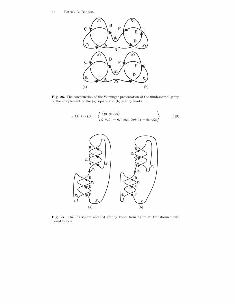
44 Patrick D. Bangert
(a) (b)
Fig. 26. The construction of the Wirtinger presentation of the fundamental groupof the complement of the (a) square and (b) granny knots.
π(G) ≈ π(S) =
⟨{g1, g2, g3} |g1g2g1 = g2g1g2; g2g3g2 = g3g2g3
⟩(49)
(a) (b)
Fig. 27. The (a) square and (b) granny knots from figure 26 transformed intoclosed braids.
Braids and Knots 45
Even though the knot groups are isomorphic, the knots are distinct. Thiscan seen by deforming the knots into closed braids and computing their Jonespolynomials. The transformation is straightforward and the result is shownin figure 27. Reading off from the figure, we obtain that
G ≈ σ−31 σ3
2 ; S ≈ σ31σ
32 (50)
Recalling the algorithm to compute the Jones polynomial yields
VGt = 3− (t3 + t−3
)+(t2 + t−2
)− (t + t−1
); VS(t) =
(t + t3 − t4
)2(51)
and we see that the knots are distinct proving that the fundamental group isa incomplete invariant.
Peripheral Group System The fundamental group is not a complete in-variant but it is possible to refine our methods to construct a complete in-variant from the fundamental group, the peripheral group system. This is theonly complete invariant of knots that we can readily compute for all knots.The problem is that distinguishing knots via the peripheral group systemrequires distinguishing groups with respect to isomorphism which is knownto be an undecidable problem [2, 3, 64].
The complement of a knot is uniquely specified (up to isomorphism) byits peripheral group system which consists of the fundamental group anda few subgroups thereof (this is Waldhausen’s theorem [73], see [40] for amore accessible proof). It is however known that the word problem for anyfundamental group of any knot is solvable [74]. If the knot is alternating, theconjugacy problem is also solvable [5].
We define the linking number of two curves a and b, denoted by lk(a, b)as the weighted sum of the characteristics ε of each crossing. We define ameridian mi and a longitude li of a knot component Ki by requiring thefollowing properties: (1) mi and li are oriented, polygonal, simple and closedcurves in ∂V (Ki), the boundary of the thickened neighborhood of Ki whichwe denote by V (Ki), (2) mi and li intersect in exactly one point, (3) mi is nullhomologous (mi ∼ 0) in V (Ki) and li ∼ Ki in V (Ki), (4) li ∼ 0 in C (Ki)and (5) lk (mi, Ki) = 1 and lk (li, Ki) = 0 in S3. The above five propertiesdefine mi and li uniquely up to isotopy on the boundary of V (K) [?] (seefigure 28 for an illustration). The meridian-longitude system pair M(K) fora j-component knot K is the pair of sets ({m1, m2, · · · , mj}, {l1, l2, · · · , lj}).Interestingly, if the longitude is trivial (equivalent to the identity element)in the knot group, the group is infinite cyclic; i.e. the group is isomorphic tothe fundamental group of the complement of the unknot. Furthermore, themeridians and longitudes commute with each other in any knot group [49].
The meridians can be taken as the Wirtinger generators of the knot group.The longitude of a knot may be read off the projection very easily. Begin withthe first generator and traverse the knot in the direction of its orientation.

46 Patrick D. Bangert
Fig. 28. The thick curve displays the trefoil knot with an orientation. The thincurve which is parallel to the trefoil knot is the longitude; the orientation of thelongitude is the same as the knot. The thin curve encircling both trefoil and longi-tude at the top left hand corner is the meridian. Note that the five conditions givenin the text are fulfilled by these curves.
Whenever undercrossing an arc, write down the generator of the undercrossedarc to the power of the negative of the characteristic of the crossing. After thefull traversal, append as many copies of the initial generator (or its inverse)to make the total sum of exponents equal to zero.
The meridians and longitudes ofM(K) may be considered to be elementsof π(K) by choosing a path pi in C(K) from the base point x0 to the (uniqueby definition) point mi∩li for each i. Then the subgroup 〈mi, li〉 of π(K), gen-erated by mi and li is independent of the choice of pi up to conjugation. Theperipheral group system of a j-component knot K is p(K) = (π(K);M(K)).By an isomorphism φ between two peripheral group systems p (K) ≈φ p (K ′),we mean π (K) ≈ π (K ′) such that φ (mi) = m′
i and φ (li) = l′i for all i. Itcan be shown that for any two knots K1 and K2, p (K1) ≈ p (K2) if and onlyif K1 ≈ K2 [49]. If we restrict attention to prime knots of a single component,we have π (K1) ≈ π (K2) if and only if K1 ≈ K2 [49]. Thus the problem ofknot isotopy can be transformed into the problem of peripheral group systemisomorphism. Since it is not possible to determine, in general, if two groupsare isomorphic, this does not solve the knot classification problem.
4 Classification of Braids and Knots
In this section we will discuss the word, conjugacy, Markov and minimal wordproblems introduced in section 2.8 in detail. There are a number of distinctsolutions to the word and conjugacy problems in Bn each of which has specialfeatures and gives additional insight into the problem and braids in general.We shall discuss briefly the solutions due to Garside as they are historicallythe most important ones and have had ground-breaking influence on the field.Then we shall discuss a new solution to both problems. The Markov problemis unsolved at present but we will discuss some of its features and why it is so

Braids and Knots 47
difficult. Lastly, we will present a number of results about the minimal wordproblem. It is computationally expensive to solve (NP-Complete) and so wepresent a heuristic algorithm and some simulation approaches and interestingresults arising from them.
4.1 The Word Problem I: Garside’s Solution
In the Artin presentation, the word problem asks whether two n-braid wordsα = σε1
a1σε2
a2· · ·σεo
aoand β = ση1
b1ση2
b2· · ·σηp
bpsuch that 1 ≤ ai, bj < n and
εi, ηj = ±1 for 1 ≤ i ≤ o and 1 ≤ j ≤ p are equivalent to each other (denotedα ≈ β) under the equations σiσj ≈ σjσi for |i − j| > 1 and σiσi+1σi ≈σi+1σiσi + 1. This problem is traditionally approached by trying to find analgorithm which will use the two braid group relations to construct, from anybraid, a unique normal form. A unique normal form α of the braid α and thecorresponding form β of the braid β are exactly equal (α = β) if and only ifα ≈ β.
Artin was the first to describe a normal form to solve the word problemfor braids [7] but the normal form has a exponentially growing number ofcrossings in terms of the original number of crossings and so is not as usefulas other methods. Garside constructed another unique normal form whichhas many important properties [37]. Garside’s method begins with the crucialproposition,
Proposition 4.1. For any σ−1i , we have σ−1
i ≈ Δ−1n Δn−1dn−1,i+1di−1,1.
Together with the fact that σiΔn ≈ Δnσn−i (see proposition 2.19), thismeans that we may put any n-braid word α into the form α ≈ Δ−q
n α′ whereα′ is a positive braid word and q the number of inverse generators present inα. Next we need to construct the diagram D(α′) of the positive braid α′.
Definition 4.2. The Cayley diagram D(b) (or diagram for short) of a pos-itive braid word b is the set of all braid words equivalent to b.
Because of proposition 2.21 which states that two positive and equal braidwords are positively equal, the following algorithm obviously constructs D(b)given a positive b.
Algorithm 4.3 Input: A positive braid word b. Output: The diagram D(b)of b.
1. We define the set D0(b) by D0(b) = {b}.2. The set Di(b) is obtained from the set Di−1(b) by adding to Di(b) all
the braid words which can be obtained from any member of Di−1(b) byapplying any braid group relation exactly once and the deleting all thosewhich are already contained in the sets Dj(b) for 0 ≤ j < j.
48 Patrick D. Bangert
3. Step 2 is recursively applied until an integer m is reached for whichDm(b) = ∅. It is obvious from the construction of the sets that a finite malways exists.
4. The set D(b) is then the union of the Di for 0 ≤ i ≤ m.
We note that, in general, D(b) contains a number of elements which growsexponentially both with the length and number of strings in b. Once D(α) hasbeen fully enumerated we select from it a word of the form Δp
nα′′ for whichp is maximal. Then we construct D(α′′) and choose the braid word α′′′ fromD(α′′) which has the lowest integer associated with it, the decimal expansionof which is given by the concatenation of the generator indices in the braidword (σ2σ1σ3 has associated integer 213). The braid word α′′′ is called thebase of the diagram D(α′′). We define the Garside normal form of the braidα to be αG = Δp−q
n α′′′. We refer to p− q as the Garside exponent and to α′′′
as the Garside remainder. It can be shown that the Garside normal form is aunique normal form and that thus two n-braid words α and β satisfy α ≈ βif and only if αG = βG. Executing this method in practise is time-consumingdue to the size of the diagram. There exists an efficient polynomial-timealgorithm to extract the maximal number of Δn from α′ due to Jacquemard[44] which we shall not present here.
The word problem was first solved by Artin [7] and then by Garside [37].Both of these solutions were algorithmic with exponential complexity. Asmentioned above, Garside’s algorithm can be made polynomial time due to anew algorithm by Jacquemard [44] to extract braids. The word problem forbraids is important enough for many people to have studied it after Garside.The most efficient algorithm (linear in n and quadratic in L) is given in[15]. Below we present a new algorithm based on rewriting systems. It isnot as efficient as the best algorithm for the word problem but it is easilygeneralizable to the conjugacy case and it is very simple to apply. Because ofthese features, we regard it as a competitive algorithm.
4.2 The Word Problem II: Rewriting Systems
In this section we will develop a new algorithm based on rewriting systemswhich are used as a tool in theoretical computer science. We begin with afinite alphabet of constants A and a finite set of variables X . A term t is afinite ordered sequence of constants and variables t = a1a2 · · · an with n ≥ 0(i.e. empty terms are allowed) and ai ∈ A ∪ X . A word w is a finite orderedsequence of constants w = b1b2 · · · bm with m ≥ 0 and bi ∈ A. A substitutionρ for a term t is a map which assigns a word to each variable in t; the resultantword is denoted by ρt. A term rewriting system (TRS) R = {(li, ri)} is a setof ordered pairs of terms li and ri. Each ordered pair in R is referred to as arule or rewrite rule and is often written in the form li → ri; the whole TRSis sometimes denoted by →R. A TRS R = {(li, ri)} is applied to a wordw0 by determining if w0 contains the word ρli, for some substitution ρ, as

Braids and Knots 49
a subword. If and only if w0 contains ρli is ρli replaced by ρri. If → is arewrite rule, then ← is its inverse, ↔ is its symmetric closure (← ∪→) and→ is its reflexive-transitive closure (→ ◦ → ◦ · · · ◦ →). Two terms t and sare said to be joinable if there exists a term r such that t → r ← s. Anyli is called a redex and any ri is called a reduct (these are abbreviations ofreducible expression and reduced term).
A word w0 is thus rewritten into a word w1 if and only ifRmay be appliedto w0. We may generate a rewrite chain of words w0 →R w1 →R · · · in thismanner. R terminates if and only if there exists no rewrite chain of infinitelength. R is locally confluent if and only if any local divergence ← ◦ → iscontained in the joinability relation → ◦ ←. R is confluent if and only ifany divergence ← ◦ → is contained in the joinability relation → ◦ ←. Ris complete if it is confluent and terminates. If R is complete a unique normalform exists for each word [8]; the final form obtained by applying R to theword a maximum number of times.
It should be noted that the computational power of term rewriting systemsis identical to that of Turing machines, i.e. one may be simulated by the other[70]. According to the Church-Turing thesis [29], this means that any functionwhich may reasonably be termed computable is computable using a TRS.
It was proven by Birkhoff [24] that the symmetric-reflexive-transitiveclosure ↔
R of a TRS R = {(li, ri)} is equivalent to the set of equationsE = {li = ri}. It is an obvious corollary to Birkhoff’s theorem that if thereexists a complete TRS R over the alphabet A = {fi, f
−1i } for which ↔
Rcontains exactly the equations {E , fif
−1i = e, f−1
i fi = e}, then R solves theword problem for the group G = 〈{fi}, E〉. Note that R also solves the wordproblem for the monoid associated with G, i.e. the monoid obtained whenthe inverses of the generators are added to the set of generators and the factthat the generators and inverses are in fact inverses (fif
−1i = e, f−1
i fi = e)added to the set of equations.
Termination It is, in general, undecidable whether a TRS terminates or not[43]. Since any Turing machine can be modeled using a TRS this is essentiallydue to the undecidability of whether a Turing machine will stop, the TuringHalting Problem [71]. It is however decidable for a TRS without any variables[33]. Thus, in general, a termination proof is specific to a particular TRS andmust be given for it. A common strategy for proving termination is to use areduction order on the symbols involved in the TRS. We define a reductionorder <o as a strict order over the alphabet and variables of the TRS whichsatisfies:
1. compatibility: For all terms u, v for which u <o v, we have xuy <o xvyfor any terms x and y.
2. closure: For all terms u, v for which u <o v and all substitutions σ, wehave σu <o σv.
3. basis: <o is well-founded, i.e. there exists a simplest term under <o.
50 Patrick D. Bangert
If one can show that every possible rewriting operation simplifies any termwith respect to such an ordering, then the TRS terminates [32]. Furthermore,a TRS R terminates if and only if there exists a reduction order <o whichsatisfies ri <o li for every rule li → ri ∈ R [8]. This is true because every stepof the rewriting process simplifies the term and there exists a simplest term.Another useful result is that a TRS terminates if and only if it terminatesfor all instances of its redexes [34]. Some conditions under which the unionof two terminating TRSs is terminating are analyzed in [34].
Confluence Like termination, confluence is, in general, undecidable [8].However, for terminating systems there exists a mechanizable method fordeciding confluence [41] that rests on Newman’s Lemma which states thata terminating TRS is confluent if and only if it is locally confluent [62] (weshall prove a generalization of this in lemma 4.11). Local confluence can bedecided by a systematic method which searches for critical pairs in the TRS.The concept of critical pairs is difficult to trace in history; for an attempt ata historical survey see [27] and for a good technical treatment see [41].
Given a TRS R = {(li, ri)}, an overlap is a word w = abc such thatab = ρli and bc = ηlj for some words a, b and c, two (possibly equal) integersi and j and substitutions ρ and η. Clearly the overlap abc may be rewrittento both ρric and aηrj . An overlap is non-critical if the reducts are joinable,ρric ↔
R aηrj and critical otherwise. A critical pair is the (unordered) pair(ρric, aηrj) which arises from a critical overlap. It is obvious that ifR containscritical pairs, it can not be confluent. The fact that the non-existence ofcritical pairs is both a necessary and sufficient condition for local confluenceis called the Critical Pair Lemma [46]. Later we shall prove lemma 4.12 whichcontains the Critical Pair Lemma.
Completeness If we can find a reduction order for a TRS R, thereby provetermination and find that there are no critical pairs, R is complete and thussolves the word problem for ↔
R. A general procedure for what to do whenwe can not do this is called Knuth-Bendix completion from their seminalpaper [50]. Again a historical account of this procedure is tangled and [27]is an attempt to unravel it. We shall follow the common practice to call itKnuth-Bendix completion even though, by their own admittion, the initialidea was not theirs.
Suppose we have a set of equations E on an alphabet A and a total order<A (this is a reduction order) on A. Construct a TRS R from E by creatinga rule li → ri in R from the equation li = ri in E for all equations in E suchthat the rules are ordered such that li >A ri. Now ↔
R is equivalent to Eand each rule represents a simplification in terms of <A. Clearly there existsa simplest word, the empty word, and so R terminates.
If there are no critical pairs, R is locally confluent and thus complete.If there are critical pairs, order them with respect to <A and append themto R as new rules. Termination still holds and so we continue this process.
Braids and Knots 51
We may delete duplicate or redundant rules from R between the steps ofthis method to obtain a smaller TRS. If this method terminates, we have acomplete system [50] [42]. If it does not terminate, a complete system maystill exist which contains an infinite number of rules. It is possible to collect aninfinite number of rules into a finite number of rules by introducing variables.The Knuth-Bendix algorithm has been implemented by several people andcan be used to determine, in some cases, whether a complete system exists.The CiME implementation was used for this thesis [53]. Producing rules withvariables and proving the non-existence of critical pairs is, at present, beyondthe computer implementations and must be done manually.
The process described here is simplified; there are more pitfalls, in general,and the method has been considerably extended to take into account manyother features (many relevant references are in [27]). The method as describedis enough for our purposes here however and is generally enough for a wordproblem in a finitely presented group.
Having reviewed TRS’s, we are now in a position to find a TRS for theword problem in Bn. The braid group Bn is defined formally as
Bn = 〈{σ1, σ2, · · · , σn−1} : σiσi+1σi = σi+1σiσi+1;σiσj = σjσi for |i− j| > 1〉 (52)
Given a finitely presented group G = 〈X, E〉, we can define an associatedmonoid M(G) =
⟨X ∪X−1, E ∪ aa−1 = 1
⟩for any a ∈ X . It is clear that
the equivalence and conjugacy classes of the group G and the monoid M(G)are identical. In order to solve the word problem for Bn, we augment themonoid M (Bn) with the generator of the center of Bn, Δ2
n to form themonoid
M+ (Bn) = 〈{σ±11 , σ±1
2 , · · · , σ±1n−1, Δ
±2n } : Δ±2
n σi = σiΔ±2n ;
Δ±2n Δ∓2
n = σ±1i σ∓1
i = e;
σ±1i σ
±1/∓1j = σ
±1/∓1j σ±1
i for |i− j| > 1;
σ±1i σ±1
i+1σ±1i = σ±1
i+1σ±1i σ±1
i+1 〉
(53)
It is obvious from the definition of the monoid M+ (Bn) that a solution of itsword and conjugacy problems provides a solution for the word and conjugacyproblems in the group Bn.
We will use Knuth-Bendix completion upon the oriented rules of M+ (Bn)under the reduction order <b
Δ2n <b Δ−2
n <b σ1 <b σ2 <b · · · <b σn−1 <b σ−11 <b σ−1
2 <b · · · <b σ−1n−1
(54)In practice, this process is laborious and would occupy prodigious space ifdescribed in detail. For this reason, we will simply state the result and proveit to be correct.
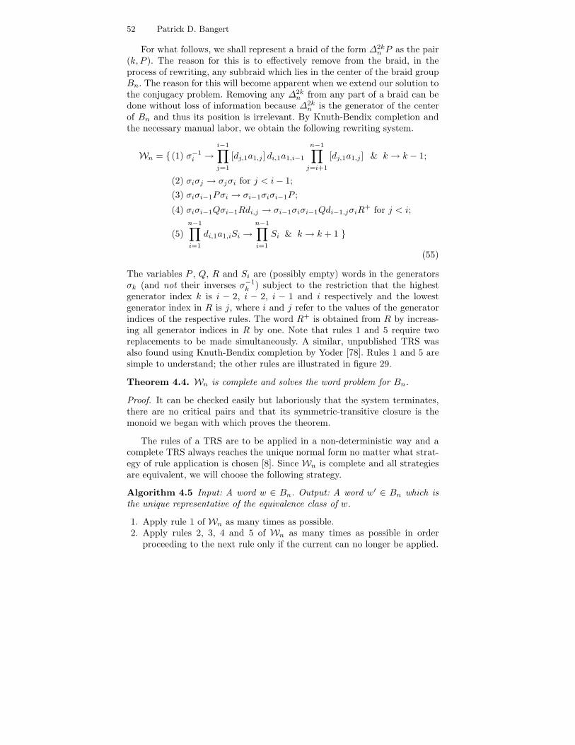
52 Patrick D. Bangert
For what follows, we shall represent a braid of the form Δ2kn P as the pair
(k, P ). The reason for this is to effectively remove from the braid, in theprocess of rewriting, any subbraid which lies in the center of the braid groupBn. The reason for this will become apparent when we extend our solution tothe conjugacy problem. Removing any Δ2k
n from any part of a braid can bedone without loss of information because Δ2k
n is the generator of the centerof Bn and thus its position is irrelevant. By Knuth-Bendix completion andthe necessary manual labor, we obtain the following rewriting system.
Wn = {(1) σ−1i →
i−1∏j=1
[dj,1a1,j ] di,1a1,i−1
n−1∏j=i+1
[dj,1a1,j] & k → k − 1;
(2) σiσj → σjσi for j < i− 1;(3) σiσi−1Pσi → σi−1σiσi−1P ;
(4) σiσi−1Qσi−1Rdi,j → σi−1σiσi−1Qdi−1,jσiR+ for j < i;
(5)n−1∏i=1
di,1a1,iSi →n−1∏i=1
Si & k → k + 1 }
(55)
The variables P , Q, R and Si are (possibly empty) words in the generatorsσk (and not their inverses σ−1
k ) subject to the restriction that the highestgenerator index k is i − 2, i − 2, i − 1 and i respectively and the lowestgenerator index in R is j, where i and j refer to the values of the generatorindices of the respective rules. The word R+ is obtained from R by increas-ing all generator indices in R by one. Note that rules 1 and 5 require tworeplacements to be made simultaneously. A similar, unpublished TRS wasalso found using Knuth-Bendix completion by Yoder [78]. Rules 1 and 5 aresimple to understand; the other rules are illustrated in figure 29.
Theorem 4.4. Wn is complete and solves the word problem for Bn.
Proof. It can be checked easily but laboriously that the system terminates,there are no critical pairs and that its symmetric-transitive closure is themonoid we began with which proves the theorem.
The rules of a TRS are to be applied in a non-deterministic way and acomplete TRS always reaches the unique normal form no matter what strat-egy of rule application is chosen [8]. Since Wn is complete and all strategiesare equivalent, we will choose the following strategy.
Algorithm 4.5 Input: A word w ∈ Bn. Output: A word w′ ∈ Bn which isthe unique representative of the equivalence class of w.
1. Apply rule 1 of Wn as many times as possible.2. Apply rules 2, 3, 4 and 5 of Wn as many times as possible in order
proceeding to the next rule only if the current can no longer be applied.
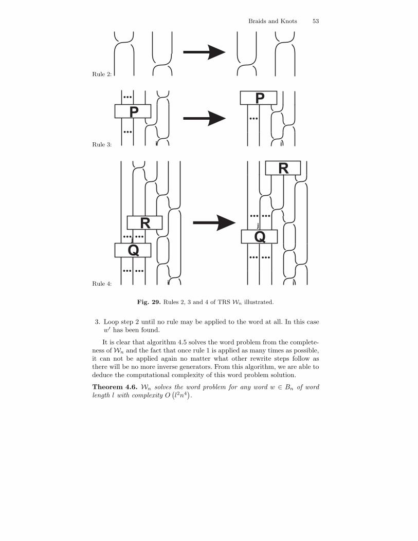
Braids and Knots 53
Rule 2:
Rule 3:
Rule 4:
Fig. 29. Rules 2, 3 and 4 of TRS Wn illustrated.
3. Loop step 2 until no rule may be applied to the word at all. In this casew′ has been found.
It is clear that algorithm 4.5 solves the word problem from the complete-ness ofWn and the fact that once rule 1 is applied as many times as possible,it can not be applied again no matter what other rewrite steps follow asthere will be no more inverse generators. From this algorithm, we are able todeduce the computational complexity of this word problem solution.
Theorem 4.6. Wn solves the word problem for any word w ∈ Bn of wordlength l with complexity O
(l2n4
).

54 Patrick D. Bangert
Proof. This can be checked easily by counting how many times the rules areused.
4.3 The Conjugacy Problem I: Garside’s Solution
Extending the word problem solution of Garside to the conjugacy case is nothard. First we define two new terms.
Definition 4.7. If a positive word b = if for two braid words i and f suchthat 1 ≤ L(i) ≤ L(b), then i is called an initial route of b and f an associatedfinal route. Note that the definition requires exact equality (=) and not grouptheoretic equivalence (≈).
We begin by constructing all possible initial routes of Δn. This is easilydone using D(Δn). Replace all of these routes by the base of their diagramsand delete duplicates. This is the set of initial routes of Δn and denoted byI (Δn).
We will now form a set S(β) for a braid word β called the summit set ofthe braid. This set is the analogue of the Cayley diagram, which we used forthe word problem, for the conjugacy problem. We construct the summit setas follows. First construct the Garside normal form of β, i.e. βG, and note itsexponent. The set S1(β) is then constructed by conjugating βG by each wordof I (Δn), computing the Garside normal form of the result and deleting allthose words of lower exponent than βG. Iteratively, the set Si(β) is obtainedfrom the set Si−1(β) by conjugating each element of Si−1(β) by each wordof I (Δn), computing the Garside normal form of the result and deleting allthose words of lower exponent than βG.
Suppose the Garside exponent of βG is m and its exponent sum is s.Every word in any Si(β) has exponent sum s and Garside exponent p ≥ mby definition. The Garside remainder of βG is βG and so we have
s = L(βG
)−mL (Δn) (56)
m =L(βG
)− s
L (Δn)(57)
p ≤ s− L(βG
)L (Δn)
(58)
but we also have p ≥ m and so there are only finitely many p that satisfy therequirements. Hence there are only finitely many distinct words with Garsideexponent p and exponent sum s. Thus the process of constructing the setsSi(β) terminates, i.e. there exists a finite integer j such that Sj(β) = Sj+1(β).
Definition 4.8. We define the summit set S(β) to consist of all the elementsof Sj(β) which have maximal Garside exponent. The summit exponent t isthe Garside exponent of all these braid words and the summit remainder is

Braids and Knots 55
the Garside remainder βS of the unique element in S(β) with smallest tail.The summit form of β is then βS = Δt
nβS.
We state, without proof, the main result of Garside.
Theorem 4.9 (Garside’s Conjugacy Theorem [37]). Two braid wordsβ1, β2 ∈ Bn are conjugate if and only if their summit forms are identical.
Proof. For a proof, see [37, 14].
Like the word problem, the conjugacy problem is very important for braidand knot theory and so has received much attention. The first solution wasproduced by Garside [37] and the best algorithms are given in [15, 36]. Weshould remark that Jacquemard [44] has used his extraction algorithm toobtain good practical results for small n. All these algorithms still requirean exponential amount of computation time as a function of n and L. Theimportant question of whether conjugacy is solvable in polynomial time issolved positively in the next section.
4.4 The Conjugacy Problem II: Rewriting Systems
Conjugacy in Free Groups Suppose that G = Fn the free group of rankn. This group is generated by n elements {fi} for 1 ≤ i ≤ n and no relations[45]. A general word w ∈ Fn takes the form
w = fp1s1
fp2s2· · · fpm
sm, 1 ≤ sk ≤ n (59)
Since there are no relations in Fn, the word w is unique over its equivalenceclass if and only if si �= si+1 for all i. This condition is trivially obtained fromany word w ∈ Fn by applying the (obviously) complete rewriting system
Rw (Fn) = {fps f q
s → fp+qs , ∀1 ≤ s ≤ n} (60)
Thus Rw (Fn) solves the word problem in any free group Fn. Moreover, itdoes so in a time proportional to the length of the word w.
Consider now the conjugacy problem in Fn. We define the ith cyclic per-mutation Ci(w) of a word w in the general form of equation (59) by
Ci(w) = fp′
jsj · · · fpm−1
sm−1fpm
smfp1
s1fp2
s2· · · fp′′
jsj (61)
such that
p′j +m∑
k=j+1
pk = i (62)
Intuitively, the ith cyclic permutation is obtained by taking the last i gener-ators in the word w and moving them to the front of the word w one by one.We shall say that two words w and w′ are cyclicly permutable (denoted ≈cp)if and only if there exist an i such that Ci(w) ≈ w′. It is obvious that cyclicpermutability forms an equivalence relation for any group G.

56 Patrick D. Bangert
Proposition 4.10. For any group G, the equivalence relation of cyclic per-mutability (≈cp) is identical to that of conjugacy (≈c).
Proof. Any group G has a presentation which may be obtained from somefree group Fn of rank n by adding relations [31]. Moreover, if the conjugacyproblem is solvable in one representation, it is solvable in all [57]. Supposew ≈cp w′, then there exists an i for which
w′ ≈ Ci(w) = fp′
jsj · · · fpm−1
sm−1fpm
smfp1
s1fp2
s2· · · fp′′
jsj (63)
where
p′j +m∑
k=j+1
pk = i (64)
Letγ = fp1
s1fp2
s2· · · fp′′
jsj (65)
Then
w′ ≈ fp′
jsj · · · fpm−1
sm−1fpm
smγ (66)
≈ γ−1γfp′
jsj · · · fpm−1
sm−1fpm
smγ (67)
≈ γ−1wγ (68)
Thus we have w ≈c w′. Now suppose w ≈c w′, then there exists a γ such that
w′ ≈ γ−1wγ (69)
If the word length of γ is L(γ), then we have
CL(γ)(w′) ≈ γγ−1w ≈ w (70)
Thus w ≈cp w′. �
We will refer to the set of words which contains the word w and all itscyclic permutations as the cyclic word c(w). If L(w) = m, then this setcontains |c(w)| = m elements. Given two cyclic words c(w) and c(w′) we testtheir equivalence by attempting to construct an isomorphism ι : c(w)→ c(w′)such that ι(a) = a for all a ∈ c(w). Clearly |c(w)| = |c(w′)| is a necessarycondition for the existence of ι. If and only if ι exists, the cyclic words areconsidered equal, c(w) = c(w′). If and only if c(w) = c(w′), we have w ≈c w′
by proposition 4.10. The set c(w) may be visualized as the word w ”madecircular” as in figure 30.
The existence of ι may be established by testing the members of c(w)for equality with the members of c(w′) pairwise in the following manner:Select from c(w) an arbitrary member, a say. Check a for equivalence withall members of c(w′). Clearly, if and only if there exists a b ∈ c(w′) suchthat a = b, an ι exists. Since every word has length m and there are mwords in c(w′), this comparison will take a time proportional to m2. Thusit is possible to test the equivalence of two cyclic words of length m withcomplexity O
(m2
).
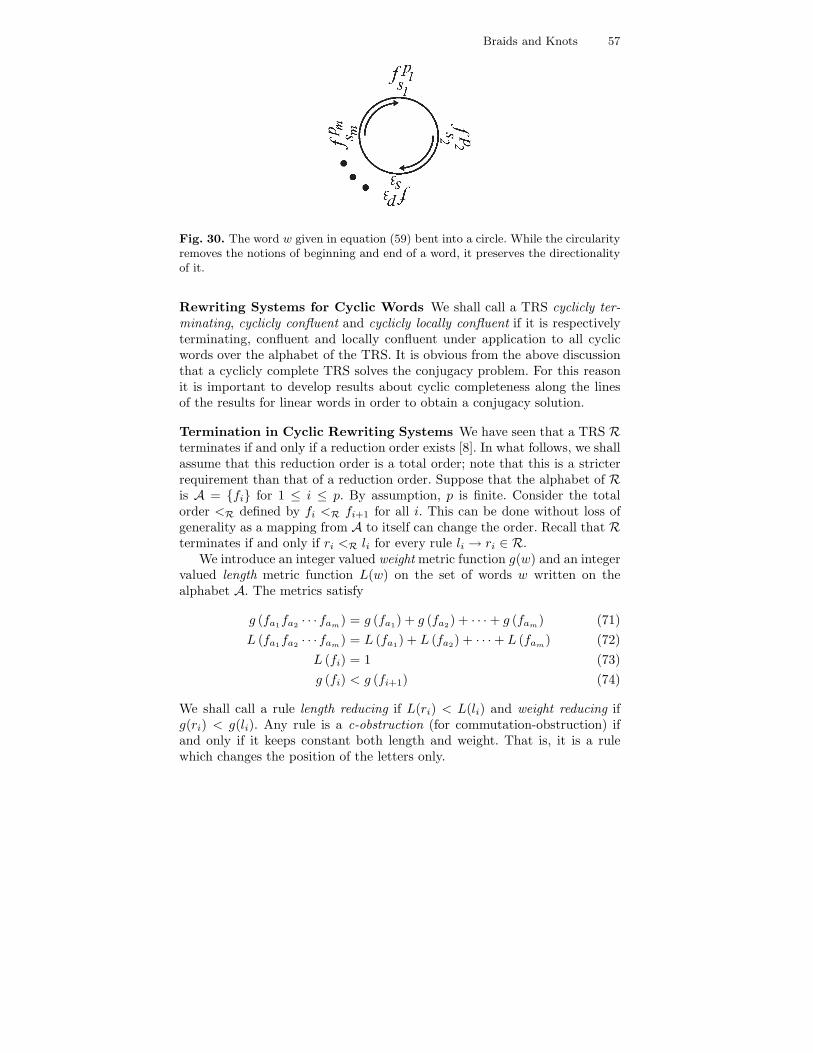
Braids and Knots 57
Fig. 30. The word w given in equation (59) bent into a circle. While the circularityremoves the notions of beginning and end of a word, it preserves the directionalityof it.
Rewriting Systems for Cyclic Words We shall call a TRS cyclicly ter-minating, cyclicly confluent and cyclicly locally confluent if it is respectivelyterminating, confluent and locally confluent under application to all cyclicwords over the alphabet of the TRS. It is obvious from the above discussionthat a cyclicly complete TRS solves the conjugacy problem. For this reasonit is important to develop results about cyclic completeness along the linesof the results for linear words in order to obtain a conjugacy solution.
Termination in Cyclic Rewriting Systems We have seen that a TRS Rterminates if and only if a reduction order exists [8]. In what follows, we shallassume that this reduction order is a total order; note that this is a stricterrequirement than that of a reduction order. Suppose that the alphabet of Ris A = {fi} for 1 ≤ i ≤ p. By assumption, p is finite. Consider the totalorder <R defined by fi <R fi+1 for all i. This can be done without loss ofgenerality as a mapping from A to itself can change the order. Recall that Rterminates if and only if ri <R li for every rule li → ri ∈ R.
We introduce an integer valued weight metric function g(w) and an integervalued length metric function L(w) on the set of words w written on thealphabet A. The metrics satisfy
g (fa1fa2 · · · fam) = g (fa1) + g (fa2) + · · ·+ g (fam) (71)L (fa1fa2 · · · fam) = L (fa1) + L (fa2) + · · ·+ L (fam) (72)
L (fi) = 1 (73)g (fi) < g (fi+1) (74)
We shall call a rule length reducing if L(ri) < L(li) and weight reducing ifg(ri) < g(li). Any rule is a c-obstruction (for commutation-obstruction) ifand only if it keeps constant both length and weight. That is, it is a rulewhich changes the position of the letters only.

58 Patrick D. Bangert
A c-obstruction obstructs cyclic termination as there exist cyclic wordswhich would give rise to an infinite rewriting chain due the changing of rel-ative position of subwords by the c-obstruction. An example is the cyclicword c(αβαβ) under the TRS R = {αβ → βα}. The rewriting chain willloop between the two states c(αβαβ) and c(βααβ); the period of the loopmay, in general, be arbitrarily large. Such looping may be dealt with in twoways. Firstly, one may compare each new cyclic word with the entirety ofthe rewrite chain so far enumerated. If equality is found, looping has beendetected and one may stop. Secondly, one may determine if a subword of thecurrent word commutes with the rest of the word. If this can be determinedand such a subword is found, the subword may be extracted from the wordand the two words should then be rewritten separately. The first method iscomputationally expensive and does not produce a unique normal form as wewould have to consider the entire loop at the end of the rewrite chain as theidentifying set of the word. The second method is not necessarily applicablebut if it is, it will terminate in a set of subwords which uniquely identify theword. The advantage of the second method over the first is that the numberof elements in the set has an upper bound.
The braid groups, as we have seen, have non-trivial center. In fact thegenerator of the center contains every generator. This fact makes it possibleto rewrite any inverse generator in terms of inverses of the generator of thecenter multiplied by generators. As in the word problem case, we shall removethe generators of the center from the word and thus this replacement rewritesthe entire braid word with which we shall work in terms of generators only.For the splitting of words to get rid of c-obstructions to fail we need to bein a situation in which we have a word abc such that abc ≈ cab, ab ≈ ba,ac �≈ ca, bc �≈ cb. This can only occur if there is cancellation between a andb in the word ab but this can not happen if there are no inverse generators.This proves that in groups in which inverse generators may be replaced byinverses of elements of the center and generators, this method of overcomingc-obstructions is valid.
We conjecture that a TRSR cyclicly terminates if and only if it terminatesand contains no c-obstructions or contains c-obstructions that can be removedin the above way.
Confluence in Cyclic Rewriting Systems Newman’s Lemma [62] ex-tends easily to the cyclic case as we show below.
Lemma 4.11. A cyclicly terminating TRS R is cyclicly confluent if andonly if it is cyclicly locally confluent.
Proof. The proof is similar to the standard proof (see [41]) and follows im-mediately from figure 31.
The Critical Pair Lemma states that a TRS is locally confluent if and onlyif it has no critical pairs. Recall that a critical pair arises from an overlap

Braids and Knots 59
Fig. 31. The proof of Newman’s Lemma (lemma 4.11) in diagrammatic form. Webegin at the top with a local divergence which is rectifiable by assumption andthus by induction any global divergence is also rectifiable. It is because of thisdiagrammatic proof that Newman’s Lemma is also known as the Diamond Lemma.
of two redexes in a word which gives rise to a local divergence of rewritingpaths which do not meet again. Given a TRS R = {(li, ri)}, a cyclic overlapis a cyclic word c(w) = c(abcd) such that abc = ρli and cda = ηlj for somewords a, b, c and d, two (possibly equal) integers i and j and substitutions ρand η. The cyclic overlap c(abcd) is rewritten to both c(ρrid) and c(bηrj). Acyclic overlap is non-critical if the reducts are joinable, c(ρrid) ↔
R c(bηrj)and critical otherwise. A cyclic critical pair is the (unordered) pair of cyclicwords (c(ρrid), c(bηrj)) which arises from a cyclic critical overlap. It is obviousthat if R contains cyclic critical pairs, it can not be cyclicly confluent.
For example, consider the rewrite system R = {abxba→ cxc} over the al-phabetA = {a, b, c} and some variables x and y. ClearlyR contains the cycliccritical overlap abxbabyb which is to be rewritten into bxbcyc and cxcbyb. Thiscyclic critical pair may be resolved by noting that if the variable containedbetween the c letters is less than the other, it is that cyclic word which isto be prefered under the lexicographic order c < b < a. That is, we have toadd a conditional rule depending on the relative value of the variables. Thisglobal rule must be applied, if applicable, with preference over the ordinarylocal rule. In this way we have extended Knuth-Bendix completion to thecyclic case; note that all rules added in this procedure are global whereas theusual rules of normal TRS’s are local. We shall now prove the extention ofthe Critical Pair Lemma for the cyclic case.
Lemma 4.12. A TRS R = {(li, ri)} is cyclicly locally confluent if and onlyif it contains neither critical nor cyclicly critical pairs.
Proof. This can easily be checked by going through all possible types ofoverlap.
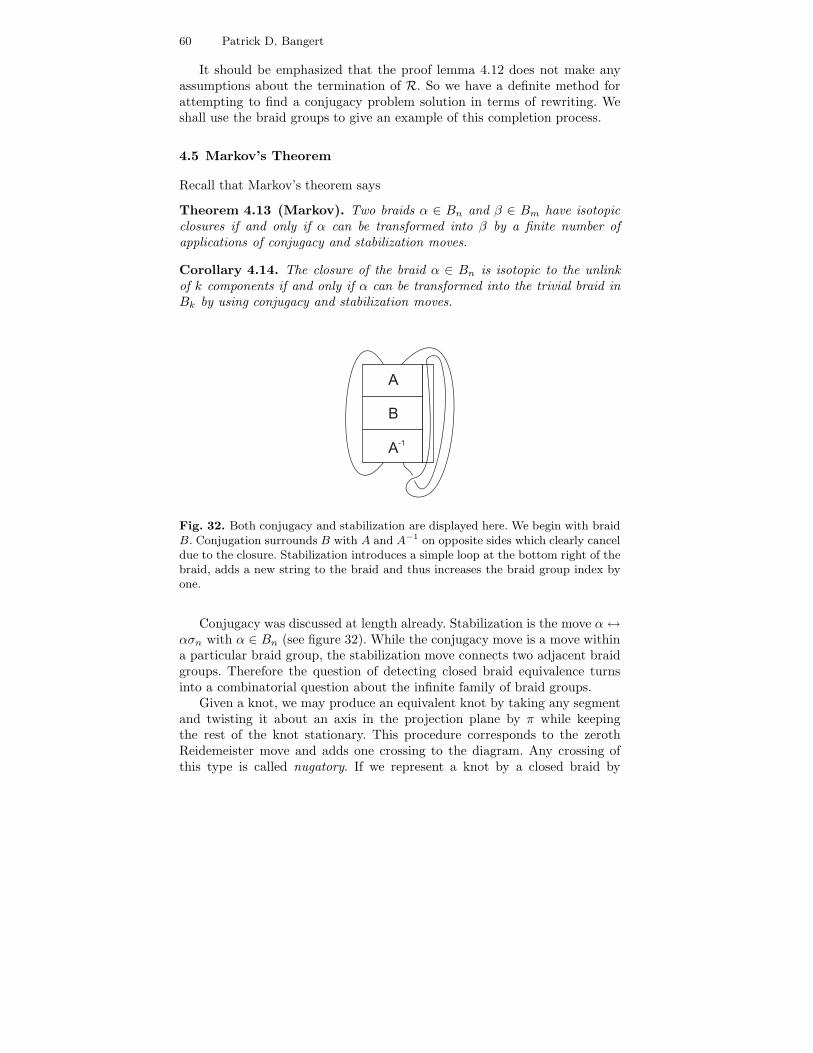
60 Patrick D. Bangert
It should be emphasized that the proof lemma 4.12 does not make anyassumptions about the termination of R. So we have a definite method forattempting to find a conjugacy problem solution in terms of rewriting. Weshall use the braid groups to give an example of this completion process.
4.5 Markov’s Theorem
Recall that Markov’s theorem says
Theorem 4.13 (Markov). Two braids α ∈ Bn and β ∈ Bm have isotopicclosures if and only if α can be transformed into β by a finite number ofapplications of conjugacy and stabilization moves.
Corollary 4.14. The closure of the braid α ∈ Bn is isotopic to the unlinkof k components if and only if α can be transformed into the trivial braid inBk by using conjugacy and stabilization moves.
A
B
A-1
Fig. 32. Both conjugacy and stabilization are displayed here. We begin with braidB. Conjugation surrounds B with A and A−1 on opposite sides which clearly canceldue to the closure. Stabilization introduces a simple loop at the bottom right of thebraid, adds a new string to the braid and thus increases the braid group index byone.
Conjugacy was discussed at length already. Stabilization is the move α↔ασn with α ∈ Bn (see figure 32). While the conjugacy move is a move withina particular braid group, the stabilization move connects two adjacent braidgroups. Therefore the question of detecting closed braid equivalence turnsinto a combinatorial question about the infinite family of braid groups.
Given a knot, we may produce an equivalent knot by taking any segmentand twisting it about an axis in the projection plane by π while keepingthe rest of the knot stationary. This procedure corresponds to the zerothReidemeister move and adds one crossing to the diagram. Any crossing ofthis type is called nugatory. If we represent a knot by a closed braid by
Braids and Knots 61
virtue of Alexander’s theorem, we may also add such nugatory crossings viaa combinatorial move, called the Markov or stabilization move. Stabilizing abraid α ∈ Bn corresponds to the operation α→ ασ±1
n or its inverse. Clearlystabilization increases or decreases the number of strings in the braid and sorepresents a move in the family of braid groups as opposed to the conjugacyand equivalence moves which are contained in a single braid group.
Markov stated in 1935 [55] that two closed braids are topologically equiva-lent if and only if they differ by stabilization and conjugacy moves (recall thatconjugacy contains equivalence). This statement became known as Markov’stheorem and was first proven in [14]. In its original form, Markov’s theoremassumes that the closed braid is embedded in S3 or R3, this can however, begeneralized to an arbitrary 3-manifold [51]. Markov’s theorem transforms thelink isotopy problem to a combinatorial question about braids. If two braidsα ∈ Bn and β ∈ Bm (with n and m possibly different) are related by stabi-lization and conjugacy, they are called Markov equivalent which is denoted by≈M . The decision problem of whether α ≈M β is called the Markov problemor the algebraic link problem. It is possible to find a single move of whichboth stabilization and conjugacy are special cases and to formulate, in thisway, Markov equivalence in terms of this so called L-move [52]. While thisL-move is intuitive, it is not obvious whether the problem has been simplifiedby this reformulation.
The first question which arises is whether there exist non-conjugateMarkov equivalent braid words in the same braid group, that is whethera solution to the conjugacy problem will solve the Markov problem. Thisis negatively resolved by showing that the two 4-braids α = σm
1 σn2 σp
1 andβ = σm
1 σp2σn
1 with m, n, p different, odd and at least three in absolute valueare not conjugate but Markov equivalent [61]. It might be thought that itshould be possible to reduce the number of strings in a closed braid equiva-lent of the unknot to one. This is true as all equivalent closed braids can bereached from each other via Markov’s theorem but the transition involves,in general, increasing the number of strings before they may be reduced toa single string. In other words, a greedy reduction of strings does not reachthe minimum string number, also known as the braid index (not even for theunknot representatives) [58].
It is a practical observation that finding a series of moves to demonstratethe Markov equivalence of two closed braids is very difficult. The difficultyof finding such a sequence has lead Birman to believe that it may be simplerto solve Markov equivalence for two braids representing prime knots. Whilethis may be true, it is not, in general, easy to decide whether a braid rep-resents a prime knot. Schubert [67] proved that the factorization sequenceof a composite knot is unique and has found an algorithm [68] which findsit. This algorithm, consequently, is able to decide whether a knot is prime.However, the execution of the algorithm rests on Hemion’s algorithm sinceit must identify the prime factors of the knot, thus no longer necessitating a

62 Patrick D. Bangert
solution of the Markov problem since it already solves the link isotopy prob-lem (albeit impractically so). This also shows that this method of decidingprimality is not practical. Birman conjectures that a braid represents a primeknot if and only if it is not conjugate to a split braid.
Furthermore, if Birman’s conjecture is true and we were to find an al-gorithm to decide whether a braid was conjugate to a split braid, we wouldhave to solve the Markov problem for this restricted class of braids. If thiscould be done, we would have a solution to the Markov problem since everybraid could be decomposed into its split components and pair-wise tested fornon-split Markov equivalence. This would not only resolve isotopy but alsogive the unique prime knot factorization of the knots. Birman’s conjectureis unproven and there exists no algorithm to test whether a braid is conju-gate to a split braid. It is possible, however, to solve the Markov problem forcertain quotient groups of the braid groups [23].
Since the word and conjugacy problems are contained in the Markov prob-lem, solutions for these are desirable and have been given numerous times asmentioned before. The stabilization move represents the final hurdle beforelink isotopy is algorithmically decidable and thus it would be interesting toknow when a braid α ∈ Bn+1 is conjugate to a braid γσ±1
n where γ con-tains only the generators σi for 1 ≤ i ≤ n − 1, for then one could reduce αto γ using the Markov move. While this has been done [56], the algorithmdepends on Garside’s conjugacy algorithm [37] which has exponential com-plexity. Moreover, if two braids were reduced in this way to the minimumstring number, they are not, in general, conjugate in this final braid group ifthey are Markov equivalent and thus this decision procedure does not solvethe Markov problem either.
We have defined the exponent sum exp(α) of a braid α as the sum ofthe exponents of the Artin generators of α. It is obvious that the exponentsum is a conjugacy class invariant but not a Markov class invariant becauseof stabilization. Thus it is possible for two braids to be Markov equivalentand have different exponent sums. In getting from one braid to the other,the exponent sum must be made equal somewhere in the chain of moves;this can clearly only be accomplished using stabilization. Stabilization canincrease or decrease the exponent sum depending whether we add σn or σ−1
n
or remove either of these. It also changes the number of strings. We may thinkthat starting from a positive braid, we should be able to reach any Markovequivalent positive braid by going through a pure positive sequence of braids;that is, we may think that positive Markov equal braids are positively Markovequal. We note that this would only be possible if the difference in exponentsum between the two braids was precisely their difference in number of strings.We conjecture that positive Markov equal braids are not positively Markovequal.
Much work was done by Birman and Menasco on various properties oflinks which could be determined from their closed braid representatives (this

Braids and Knots 63
work was published in the six-paper series [16], [17], [18], [19], [20] and [21]).They prove that there exists a complete numerical invariant for knots butfind this invariant only for knots which are closed 3-braids. The invariantfor closed 3-braids is described extensively and can be used to determinethe braid index and whether the knot is split, composite, amphicheiral orinvertible. They also define a new type of move on braids, the exchangemove, and prove a Markov-like theorem for it. See [22] for a summary of thiswork.
4.6 The Minimal Word Problem
A well-known problem of combinatorial braid theory is the minimizationproblem: Given a braid A ∈ Bn find a braid Am such that A ≈ Am andL(Am) ≤ L(A∗) for any braid A∗ ≈ A where L(A) denotes the word lengthof the braid A.
In the Artin representation of Bn, the number of generators required towrite down a braid word, its length, is equal to the crossing number of thetopological braid. In practice, we find that by moving a few of the stringsof the topological braid, its crossing number may be reduced, making thebraid simpler. It would be especially useful to possess a general method tocompute an equivalent braid of minimum crossing number. Apart from manyapplications, this problem is well-known in combinatorial braid theory andis of independent mathematical interest.
Given a braid A ∈ Bn in the Artin generators, the question whether thereexists an equivalent braid A′ ∈ Bn of shorter length has been shown to be NP-Complete by Paterson and Razborov [63]. Not only does this mean that thisquestion is computationally equivalent to all other NP-Complete problems, italso means that (unless P = NP) any algorithm which answers the questionwould execute in exponential-time in n. Since Paterson and Razborov’s resultrefers to the minimization problem for general n, we ask whether it is also anNP-complete question for particular n. This question is explicitly asked asopen question 9.5.6 on page 209 of [36] and it seems to have been negativelyanswered in an unpublished preprint by Tatsuoka five years earlier but wewere unable to obtain it [69].
In proving the NP-Completeness of the problem, Paterson and Razborovshowed that the problem can be reduced to a known NP-Complete problem.This does not however provide a usable algorithm. For 3-braids, a linearcomplexity algorithm has been found [11] but no general algorithm for n > 3exists. A minimization algorithm in the band-generator presentation of thebraids groups has been found for n = 3, 4 but the length of the braid inthis presentation is not equal to the crossing number [76] [47]. It is untypicalof a group for which the word problem is solvable that no unique normalform of minimal length in some naturally arising presentation exists for thebraid groups. A unique normal form of minimal length in certain natural

64 Patrick D. Bangert
presentations of free groups, HNN-extensions and free products exists, forexample.
After a little experimentation, it is clear that a braid must, in general, beincreased in length before it may be reduced to minimum length algebraically.We show that a certain readily obtained braid provides an upper bound forthis necessary increase in length and prove several properties of this braid.We explicitly construct a set of words which must be searched for a certainproperty in order to obtain a minimal length representative of any braid.This constitutes an algorithm to solve the minimization problem. Since theset of words which must be searched is, in the worst case, exponential in size,the algorithm takes an exponential amount of time to complete.
Exercise 4.15. Find a braid which is non-minimal in length and which mustbe increased in length (by introducing pairs like σiσ
−1i ) before it can be short-
ened to minimal length. An example is the braid σ2σ−21 σ−2
2 σ1σ−12 σ1σ
22σ1σ2.
Denote by Am any braid which satisfies Am ≈ A and L(Am) ≤ L(A∗)for all braids A∗ ≈ A. We now prove a basic lemma which connects Amax
and Am. Recall that Amax = Δ−s(A)n A′ where s(A) is the number of inverse
generators in A and A′ is positive.
Theorem 4.16. For any braid A, it is possible to obtain Am from Amax byoperations which monotonically decrease or keep constant the length of thebraid.
Proof. By construction Am ≈ Amax ≈ A and Amax and A are at least as longAm. Exponent sum is an equivalence class invariant so that s(Am) ≤ s(A).Replace each inverse generator in Am with the braid given in proposition 4.1and then use equation σiΔn = Δnσn−i to bring all the fundamental braidsto the front to obtain the braid
Ammax = Δ−s(Am)n A′
m (75)≈ Δ−s(Am)
n Δs(Am)−s(A)n Δs(A)−s(Am)
n A′m (76)
≈ Δ−s(A)n Δs(A)−s(Am)
n A′m (77)
But Amax = Δ−s(A)n A′ and since the braid groups are left-cancelative [37],
we have thatΔs(A)−s(Am)
n A′m ≈ A′ (78)
with both words positive. Since positive words are positively equal [37],there exists a sequence of braids Bi for 0 ≤ i ≤ q with B0 = A′,Bq = Δ
s(A)−s(Am)n A′
m, Bj and Bj+1 different by a single application of thebraid group’s defining relations and Bi positive for all i. Since exponent sumis an equivalence class invariant, L(Bi) = L(A′) for all i.
From Amax we may thus reach the form of Ammax in equation (77) keepingthe length of the braid constant. From this form, we may reach Am by opera-tions which monotonically decrease or keep constant the length of the braid.

Braids and Knots 65
Thus there exists a sequence of braids Wi for 1 ≤ i ≤ p with W0 = Amax,Wp = Am, Wj and Wj+1 different by a single application of the braid group’sdefining relations and L(Wj+1) ≤ L(Wj), which proves the lemma. �
Theorem 4.16 basically establishes that we may reach a minimum lengthrepresentative from Amax by rearranging and cancelling generators only; itthus, in principle, removes the difficulty we pointed out in the introductionof occasionally having to increase the length before being able to decrease itto an absolute minimum.
We present an extension to the Cayley diagram construction which drawsthe diagram of any braid word (as opposed to positive braid words only).The diagram is a list of all those braid words which may be obtained fromthe given word by rearranging only.
Algorithm 4.17 Input: A braid word A. Output: A list D(A) of all braidwords B which may be obtained from A by rearranging of generators only.
1. Define the diagram of zeroth order as the set D0(A) = {A}.2. The set Di(A) is obtained from the set Di−1(A) by the following proce-
dure:a) Fix attention on a particular member α of Di−1(A). We read α from
left to right and decide at each position whether we may apply anyof the moves in equations (79) to (82).
σiσj ↔ σjσi for |i− j| > 1 (79)σiσi+1σi ↔ σi+1σiσi+1 (80)
σiσ−1i ↔ σ−1
i σi (81)σiσ
−1i σj ↔ σjσiσ
−1i (82)
b) If we may, we apply it and store the resultant braid word β in Di(A)if and only if β is not already contained in Dj(A) for 0 ≤ j ≤ i.
c) We continue to read across α until we have considered all braid wordswhich may be reached from α by a single application of the moves inequations (79) to (82).
d) Apply steps (a) through (c) for every braid in Di−1(A). If Di(A) = ∅,then the algorithm is done.
3. The diagram D(A) of A is the union of all the Di(A),
D(A) = D0(A)⋃
D1(A)⋃· · ·
⋃Dm(A) (83)
We show the correctness and termination of this algorithm.
Lemma 4.18. Algorithm 4.17 terminates for every A and succeeds in listingall braid words B which may be obtained from A by rearranging of generatorsonly, that is using the braid group relations without introducing or removingany generators.

66 Patrick D. Bangert
Proof. D0(A) is, by definition, finite. It is obvious that for any braid wordof finite length, the moves in equations (79) to (82) may be applied a finitenumber of times. Thus, by induction, every Di(A) is finite. The number ofdistinct braid words of a given finite length is finite and since the Di(A)are, by construction, non-overlapping, their union must be finite. Thus thereexists an m such that Dm+k(A) = ∅ for every k > 0. Thus the algorithmterminates for every A.
The moves listed in equations (79) to (82) exhaust all possibilities allowedin the braid group under the stipulation that no generators must be removedfrom or introduced into the word. Thus each word which may be reached fromA by rearrangement of generators will eventually be reached by algorithm4.17 and so the algorithm succeeds in listing all the required braid words. �
Theorem 4.16 gives the following corollary.
Corollary 4.19. D(Amax) contains a braid of the form EAm for E ≈ e, theidentity in Bn.
Proof. By construction D(Amax) contains all braid words equivalent toAmax by rearranging only. By lemma 4.16, Am can be obtained by a se-quence of operations which keeps the length constant or decreases it. Eachoperation which decreases the length does so by eliminating a sub-word likeei = σiσ
−1i ≈ σ−1
i σi.Since for all i ei ≈ e, the identity in Bn, we have
eiσ±1j ≈ σ±1
j ei, eiej ≈ ejei (84)
for any i and j.Let us now agree to construct the aforementioned sequence of words with-
out eliminating the sub-words ei but using equation (84) to bring them all tothe left of the word. At the end, we will obtain a word of the form A∗ = EAm
where E ≈ e is a braid consisting of all these sub-words ei. The most generalform of E is
E = eq11 eq2
2 · · · eqn−1n−1 (85)
with qi ≥ 0 for all i. So if we could extract E from Amax, we would, in theprocess, obtain Am. Since the form EAm is obtained by rearrangements only,L(E) ≤ L(A∗) = L(Amax). This indicates that
∑n−1i=1 2qi ≤ L(Amax). �
Given a braid A, we thus find Am by constructing the diagram D(Amax)and selecting the word with the largest number of cancellation pairs such asσiσ
−1i . Clearly there will be more than one braid word for the same number
of cancellation pairs. We may agree to choose the least braid word lexico-graphically for definiteness. It is obvious from the construction that this willbe a unique form of minimal length for the braid A. We thus have an algo-rithm to find Am for any A. It is regrettable that the diagram D(Amax) is,
Braids and Knots 67
by construction, very large. Two questions are left to ask: Can we make theresult stronger and how large is a typical diagram?
In theorem 4.16 we achieved an upper bound for the necessary increase inlength of a braid before it may be reduced to a minimum length. One wouldlike to simplify the result somewhat but we shall show in this section thatthe two straightforward attempts to simplify or strengthen theorem 4.16 aredoomed to failure. First we show that we may not, in general, shorten Amax
to the Garside normal form.
Lemma 4.20. It is not, in general, possible to obtain Am from G(A), theGarside normal form of A, by operations which monotonically decrease orkeep constant the length of the braid.
One may think that it would be sufficient to list the diagram of the neg-ative and positive sub-braids of Amax and search for a maximal length sub-braid which is common to the end of the first and the beginning of the seconddiagram but this is not true as the following lemma shows.
Lemma 4.21. There does not exist an Am in the form A1A2 with A1 nega-tive and A2 positive for every A.
Let a be a n-braid of length L with diagram D(a). Consider the braida′ = aσiσ
−1i for some 1 ≤ i < n. We are concerned with the size of D(a′)
in terms of the size of D(a). For each member of D(a), the cancellation pairσiσ
−1i may appear in any place in both possible orders (σiσ
−1i and σ−1
i σi), soin 2(L+1) positions. There may be further moves possible by use of the braidgroup relations but the number of these are clearly bounded by a functionlinear in L. So the diagram of a word will increase in size by a factor linear inits length for each possible cancellation pair. Given a random positive n-braida of length L, how many members will D(a) have, on average? We conjecturethat:
Conjecture 4.22. For any braid a ∈ Bn of length L, we have that |D(a)| ≤|D(Δp
n)| with p = �2L/(n(n− 1))�.Conjecture 4.22 would provide an upper bound for the size of the diagram
of any word in terms of the diagrams of the diagrams of Δpn which topologi-
cally are a series of p half-twists of the braid strings about the vertical axis.In extensive computer simulations, the conjecture was checked and seems tohold. What it seems to indicate is that the half-twist has the most topolog-ical freedom for its length and number of strings under the constraint thatthe crossing number must be kept constant. This is quite intuitive, yet theconjecture seems to be difficult to prove.
We have investigated the diagrams of several Δpn for their size and for the
distribution of braids over the sub-diagrams at each stage of the constructionin algorithm 4.17. In table 1 we list the size of the diagram and maximalsub-diagram index for p half-twists on n strings.

68 Patrick D. Bangert
Table 1. The Size of Diagrams of Fundamental Words
n p |D (Δpn)| max. i
3 1 2 13 2 8 23 3 38 53 4 196 83 5 1062 133 6 5948 183 7 34120 254 1 16 74 2 1654 155 1 768 25
We conclude that the diagram of a typical braid word grows exponen-tially with its length and braid index and thus our method of finding theminimal length braid word equivalent to a given braid has exponential com-plexity. This is not surprising as the problem is NP-Complete. We shall givea heuristic algorithm and other methods later. The properties of the braidgroups that made the above solution possible are: (i) It is possible to write allinverse generators as products of the generator of the center and a positiveword, (ii) the defining relations relate positive words only and (iii) the braidgroups are right and left-cancellative. It is likely that any group which hasthese properties, has an analog of the Garside normal form and has a solutionto the minimum word problem similar to the one above.
Solving the problem exactly is an expensive endeavor and so we ask forapproximate methods. It turns out that magnetic relaxation is an importantapplication of this problem and gives rise to good methods to solve it. We shalldelay the discussion of these to section ??. It is possible to solve the problemheuristically using a purely algebraic algorithm which we now present.
Recall that the braid group Bn is defined by
Bn = 〈 {σi} : 1 ≤ i < n; (86)σiσj = σjσi |i− j| > 1; σiσi+1σi = σi+1σiσi+1〉 . (87)
An n-braid A of c crossings is a word in Bn of word-length c, so the generalform of A is
A = σε1a1
σε2a2· · ·σεc
acεk = ±1, 1 ≤ ak < n, ∀k : 1 ≤ k ≤ c. (88)
Consider an n-braid A of the form given in equation 88. Suppose we wishto find the n-braid Am equivalent to A such that the length L(Am) of Am
is minimal over the equivalence class of A. It has been shown [63] that thisquestion is NP-complete and hence computationally difficult (if P �= NP, it isintractable). The following presents a heuristic algorithm for getting close toAm. We begin with the leftmost generator of A and attempt to move it to the

Braids and Knots 69
right using both braid group operations. If we can cancel it along the way,we do and if we can not, we move it back to where it started. In this way,we proceed to move all the generators as far to the right as possible. Thenwe begin at the end and move each generator as far to the left as possiblein the same manner. This algorithm will always produce an equivalent braidA′ such that L(A′) ≤ L(A). We consider L(A) generators and move themO(L(A)) moves to the right and left. Thus this algorithm takes O
(L(A)2
)time and constant memory. In fact we move a particular generator at mostL(A) generators and this is only for the case when all the other generatorscommute with it, thus the average case complexity is likely to be close tolinear in L(A).
This algorithm will not produce a minimum length representative in allcases because it can not unravel complex crossings. To get to the minimumlength would require more subtle transformations than just movements tothe right or left, which topologically correspond to pulling the strings apartfrom underneath the crossing. However, as computer experiments show, itdoes do quite well.
Let us calculate an upper bound to the reduction ratio obtained by thismethod as a function of n and c. To calculate these, consider the likelihoodthat a particular generator will be followed by its inverse, which is just Q0 =1/2(n−1). The probability Qj that a generator and its inverse are separatedby j generators through which either can be moved is the correspondingprobability for j = 1 to the power j. We require the number of braids oflength 1 which may be generated so as not to contain the generator interferingwith the movement of generator σi. If i = 1 or n − 1, this is 2(n − 3) and2(n− 4) otherwise. Thus
Qj =
⎡⎣2(n− 4)
(2(n−1)−22(n−1)
)+ 2(n− 3)
(2
2(n−1)
)2(n− 1)
⎤⎦
j
Q0 (89)
=[n2 − 5n + 5
(n− 1)2
]j
Q0 (90)
The final factor of Q0 is present because the generator after the sequenceof j generators is required to be inverse of the original generator, an eventwith probability Q0. To get the total probability Q of being able to can-cel a generator σi with its inverse by simple exchange movements over thelength j = 0, 1, · · · , we must sum these probabilities in order weighted by theprobability that their predecessors did not happen. Thus
Q = Q0 + (1−Q0)Q1 + · · ·+j−1∏k=0
(1−Qk)Qj + . . . (91)
Note that since the exchange move is not allowed for n = 3, Q = Q0 for n = 3.The reduction ratio R which occurs as a consequence of this probability is

70 Patrick D. Bangert
R = 1 − 2Q since each time that the event happens two generators may becanceled. Note that in this calculation we have considered the probabilitythat a generator can be moved next to its inverse in the word using only thefar commutation relation that σiσj = σjσi for |i− j| > 1 in a long braid. Theheuristic algorithm however uses both braid group moves to attempt to movegenerators next to their inverses. Thus R is an upper bound for the reductionratio achieved by the heuristic algorithm as the braid becomes long.
In §6 we present the results of the algebraic reduction of a large numberof braids but a few comments about the efficiency of the algorithm are inorder. The only exact algorithm to minimize braid is valid only for n ≤ 3[11] and by comparing this heuristic to this exact algorithm, we find thatthe heuristic finds a braid the length of which is within five percent of thelength found by the exact algorithm and that it reaches the actual minimumin 0.005 of all cases. This shows that the heuristic is quite effective for n = 3(note that reduction for n = 1, 2 is trivial since B1, B2 are free groups).
5 OpenProblems
The problems that follow are, to the best of my knowledge, unsolved at thetime of publication. The selection is personal and far from complete. However,each problem is quite significant in that its solution will have an impact onresearch. I believe that even partial results for most of these problems wouldbe worth a Ph.D. The problems are presented in no particular order.
1. Is the Burau representation faithful for n = 4? Seems hard to answer butthe significance is somewhat debatable since it is unfaithful for n > 4.
2. Does the Jones polynomial identify the unknot? In other words, is therea knot (distinct from the unknot) that has the same Jones polynomial asthe unknot? (Warning: Searches for a counterexample have gotten quitefar in the knot tables, so if there is a counterexample it is not simple. Atpresent, it seems likely that there is no counterexample.)
3. Construct a polynomial-time algorithm for calculating the Jones andrelated polynomials or show that this cannot be done (assuming thatP �= NP a proof of NP-completeness would do).
4. Construct an inherently algebraic algorithm for solving the Markov prob-lem. (Note: The problem is definitely solvable via Hemions algorithm butthis is very complicated, we are looking for a simple algorithm even if itis in exponential-time.)
5. Prove that the Markov problem is NP-complete, intractable or find apolynomial-time algorithm for it. (Note: Depending on how this is doneand the answer, this is probably a Fields Medal problem but that shouldnot discourage you from trying it.)
6. Construct a provably secure cryptosystem on the basis of the braid orsimilar groups. (Note: With present systems the question of security isnot quite settled.)

Braids and Knots 71
7. Create a general theory of 2-tangle equations and how to solve them.(Note: The solvability needs to be practical as these equations actuallycome up in biology.) As an encore, do it for n-tangle equations.
8. Create a theory of physical braids with aims to study then tension prop-erties of various knots independent of the rope on which they are tied.
9. Construct further invariants of knots and braids, preferably easily calcu-lable and strong (not too many distinct knots having the same value ofyour invariant).
10. Construct a complete invariant of knots that can actually be comparedcomputationally. (Note: The peripheral group system is complete but itcannot be compared to other systems because groups cannot in generalbe distinguished from another.)
11. Build a software system that makes it easy to input/output knots andbraids, compute many invariants, identify the knot in a table, constructa knot table and play with new ideas largely independent of complexprogramming.
References
1. Adams, C., Hildebrand, M., Weeks, J. (1991): Hyperbolic Invariants of Knotsand Links. Trans. Amer. Math. Soc., 326, 1–56.
2. Adian, S. I. (1957): The unsolvability of certain algorithmic problems in thetheory of groups. Trudy Moskov. Mat. Obsc., 6, 231–298.
3. Adian, S. I. (1957): Finitely Presented Group and Algorithms. Dokl. Akad.Nauk SSSR, 117, 9–12.
4. Alexander, J. W. (1923): A lemma on systems of knotted curves. Proc. Nat.Acad. Sci. USA, 9, 93–95.
5. Appel, K. I. and Schupp, P. E. (1972): The Conjugacy Problem for the Group ofany Tame Alternating Knot is Solvable. Proc. Amer. Math. Soc., 33, 329–336.
6. Artin, E. (1925): Theorie der Zopfe. (in German) Abh. Math. Sem. Univ. Ham-burg, 4, 47–72.
7. Artin, E. (1947): Theory of braids. Ann. Math., 48, 101–126.8. Baader, F., Nipkow, T. (1998): Term Rewriting and All That. (Cambridge Uni-
versity Press, Cambridge).9. Bangert, P. D., Berger, M. A., Prandi, R. (2002): In Search of Minimal Random
Braid Configurations. J. Phys. A., 35, 43–59.10. Berger, M. A. (1993): Energy-crossing number relations for braided magnetic
fields. Phys. Rev. Lett., 70, 705–708.11. Berger, M. A. (1994): Minimum crossing numbers for 3-braids. J. Phys. A, 27,
6205–6213.12. Berger, M.A. (2000): Hamiltonian dynamics generated by Vassiliev invariants.
J. Phys. A., 34, 1363–1374.13. Bigelow, S. (1999): The Burau representation is not faithful for n = 5. Geometry
and Topology, 3, 397–404.14. Birman, J. S. (1974): Braids, Links and Mapping Class Groups. Ann. of Math.
Studies 82 (Princeton Univ. Press, Princeton).

72 Patrick D. Bangert
15. Birman, J. S., Ko, K. H., Lee, S. J. (1998): A New Approach to the Word andConjugacy Problems in the Braid Groups. Ad. Math., 139, 322–353.
16. Birman, J. S., Menasco, W. (1992): Studying Links Via Closed Braids I: AFiniteness Theorem. Pacific J. Math., 154, 17–36.
17. Birman, J. S., Menasco, W. (1991): Studying Links Via Closed Braids II: Ona Theorem of Bennequin. Topology and Its Applications, 40, 71–82.
18. Birman, J. S., Menasco, W. (1993): Studying Links Via Closed Braids III:Classifying Links which are Closed 3-braids. Pacific J. Math., 161, 25–113.
19. Birman, J. S., Menasco, W. (1990): Studying Links Via Closed Braids IV:Closed Braid Representatives of Split and Composite Links. Invent. Math., 102,115–139.
20. Birman, J. S., Menasco, W. (1992): Studying Links Via Closed Braids V: ClosedBraid Representatives of the Unlink. Trans. AMS, 329, 585–606.
21. Birman, J. S., Menasco, W. (1992): Studying Links Via Closed Braids VI: ANon-Finiteness Theorem. Pacific J. Math., 156, 265–285.
22. Birman, J. S., Menasco, W. (1992): A calculus on links in the 3-sphere. inKawauchi, A. Knots 90 (Walter de Gruyter, Berlin), 625–631.
23. Birman, J. S., Wajnryb, B. (1986): Markov Classes in Certain Finite Quotientsof Artin’s Braid Group. Israel J. Math., 56, 160–178.
24. Birkhoff, G. (1935): On the structure of abstract algebras. Proc. Camb. Phil.Soc., 31, 433–454.
25. Bohnenblust, F. (1947): The Algebraical Braid Group. Ann. Math., 46, 127–13626. Boyland, P. L., Aref, H., Stremler, M. A. (2000): Topological fluid mechanics
of stirring. J. Fluid Mech., 403, 277–304.27. Buchberger, B. (1987): History and Basic Features of the Critical-
Pair/Completion Procedure. J. Sym. Comp. 3, 3–38. Printed in Rewriting Tech-niques and Applications ed. by Jouannaud, J.-P. (Academic Press, London),3–38.
28. Chan, T. (2000): HOMFLY polynomials of some generalized Hopf links. J. KnotTh. Rami., 9, 865–883.
29. Cohen, D.E. (1987): Computability and Logic. (Ellis Horwood, Chichester).30. Conway, J.H. (1970): An Enumeration of Knot and Links, and Some of their
Algebraic Properties. in Leech, J. (1970): Computational Problems in AbstractAlgebra. (Pergamon, Oxford)
31. Coxeter, H.S.M., Moser, W.O.J. (1957): Generators and Relations for DiscreteGroups. (Springer, Berlin)
32. Dershowitz, N. (1979): A note on simplification orderings. Inform. Proc. Let.,9, 212–215.
33. Dershowitz, N. (1981): Termination of linear rewriting systems. in Automata,Languages and Programming ed. by Even, S. and Kariv, O., Lecture Notes inComputer Science Volume 115 (Springer, Heidelberg), 448–458.
34. Dershowitz, N. (1987): Termination of Rewriting. J. Sym. Comp., 3, 69–116.Printed in Rewriting Techniques and Applications ed. by Jouannaud, J.-P. (Aca-demic Press, London), 69–116.
35. Dowker, C. H. and Thistlethwaite, M. B. (1983): Classification of Knot Projec-tions. Top. Appl., 16, 19–31.
36. Epstein, D.B.A., Cannon, J.W., Holt, D.F., Levy, S.V.F., Paterson, M.S.,Thurston, W.P. (1992): Word Processing in Groups. (Jones and Bartlett,Boston).
Braids and Knots 73
37. Garside, F.A. (1969): The braid group and other groups. Quart. J. Math. Ox-ford, 20, 235–254.
38. Gilbert, N.D., Porter, T. (1994): Knots and Surfaces. (Oxford University Press,Oxford).
39. Hemion, G. (1992): The Classification of Knots and 3-dimensional Spaces. (Ox-ford Univ. Press, Oxford).
40. Hempel, J. (1976): 3-manifolds. Ann. of Math. Studies Volume 86 (PrincetonUni. Press, Princeton).
41. Huet, G. (1980): Confluent reductions: Abstract properties and applications toterm rewriting systems. J. Assoc. Comput. Mach., 27, 797–821.
42. Huet, G. (1981): A Complete Proof of the Knuth-Bendix Completion Algo-rithm. J. Comp. Syst. Sci., 23, 11–21.
43. Huet, G., Lankford, D.S. (1978): On the uniform halting problem for termrewriting systems. Rapport laboria 283, Institut de Recherche en Informatiqueet en Automatique, Le Chesnay, France.
44. Jacquemard, A. (1990): About the effective classification of conjugacy classesof braids. J. Pure Appl. Al., 63, 161–169.
45. Johnson, D.L. (1980): Topics in the Theory of Group Presentations. Lon. Math.Soc. Lec. Notes Vol. 42 (Cambridge Uni. Press, Cambridge).
46. Jouannoud, J.P., Kirchner, H. (1986): Completion of a set of rules modulo aset of equations, SIAM. J. Comp., 15, 1155–1194.
47. Kang, E. S. et. al. (1997): Band-generator presentation for the 4-braid group.Top. Appl., 78, 39–60.
48. Kauffman, L. (1993): Knots and Physics. Series on Knots and Everything Vol.1. World Scientific, Singapore.
49. Kawauchi, A. (1996): A Survey of Knot Theory. (Birkhauser Verlag, Basel)50. Knuth, D.E., Bendix, P.B. (1970): Simple word problems in universal alge-
bras. in Computational Problems in Abstract Algebra ed. by Leech, J. (Perga-mon Press, Oxford), 263–297. Reprinted in 1983 in Automation of Reasoning 2(Springer, Berlin), 342–376.
51. Lambropoulou, S.S.F. (1993): A Study of Braid in 3-manifolds. unpublishedPhD thesis (Univ. of Warwick).
52. Lambropoulou, S.S.F., Rourke, C.P. (1997): Markov’s Theorem in 3-manifolds.Top. Appl., 78, 95–22.
53. The CiME system is available from http://cime.lri.fr.54. Magnus, W., Peluso, A. (1967): On Knot Groups. Comm. Pure Appl. Math.,
20, 749–770.55. Markov, A.A. (1935): Uber die freie Aquivalenz geschlossener Zopfe (in Ger-
man), Recueil Mathematique Moscou, 1, 73–78. [Mat. Sb. 43 1936.]56. McCool, J. (1980): On Reducible Braids. in Word Problems II ed. by Adian,
S. I., Boone, W. W. and Higman, G. (North-Holland, Amsterdam), 261–295.57. Miller, C.F. III (1992): Decision Problems for Groups - Survey and Reflections.
in Algorithms and Classification in Combinatorial Group Theory ed. by Baum-slag, G. and Miller, C. F. III, Math. Sci. Re. Inst. Pub. Volume 23 (Springer,New York), 1–59.
58. Morton, H.R. (1983): An irreducible 4-string braid with unknotted closure.Math. Proc. Camb. Phil. Soc., 93, 259–261.
59. Morton, H.R. (1986): Threading Knot Diagrams. Math. Proc. Camb. Phil. Soc.,99, 247–260.
74 Patrick D. Bangert
60. Murasugi, K. (1996): Knot Theory And Its Applications. (Birkhauser, Boston).61. Murasugi, K., Thomas, R.S.D. (1972): Isotopic closed nonconjugate braids.
Proc. Am. Math. Soc., 33, 137–139.62. Newman, M.H.A. (1942): On theories with a combinatorial definition of ’equiv-
alence’. Ann. Math., 43, 223–243.63. Paterson, M.S., Razborov, A.A. (1991): The set of minimal braids is co-NP-
complete. J. Algorithms, 12, 393–408.64. Rabin, M.O. (1958): Recursive Unsolvability of Group Theoretic Problems.
Ann. Math., 67, 172–194.65. Reidemeister, K. (1983): Knot Theory. BCS Associates, Moscow, Idaho. Orig-
inally published as Reidemeister, K. (1932): Knotentheorie. Springer, Berlin66. Ricca, R.L. (1998): Applications of Knot Theory in Fluid Mechanics. in Jones,
V.F.R. et. al., ed. by Knot Theory Banach Center Pub. Vol. 42 (Inst. of Math.,Polish Acad. Sci., Warszawa), 321–346.
67. Schubert, H. (1948): Die Eindeutige Zerlegbarkeit eines Knotens in Primknoten.(in German), Sitz. Heidelberger Akad. Wiss., math.-nat. Kl., 55–104.
68. Schubert, H. (1961): Bestimmung der Primfaktorzerlegung von Verkettungen.(in German), Math. Zeitschr., 76, 116–148.
69. Tatsuoka, K. (1987): Geodesics in the braid group. preprint, Dept. of Mathe-matics, University of Texas at Austin.
70. Tourlakis, G.J. (1984): Computability. (Reston, Reston).71. Turing, A.M. (1937): On Computable Numbers, with an Application to the
Entscheidungsproblem. Proc. London Math. Soc. Ser. 2, 42, 230–265.72. Vogel, P. (1990): Representation of links by braids: A new algorithm. Comment.
Math. Helvetici, 65, 104–113.73. Waldhausen, F. (1968): On Irreducible 3-manifolds which are Sufficiently Large.
Ann. Math., 87, 56–88.74. Waldhausen, F. (1968): The Word Problem in Fundamental Groups of Suffi-
ciently Large Irreducible 3-manifolds. Ann. Math., 88, 272–280.75. Williams, R.F. (1988): The Braid Index of an Algebraic Link. In: Birman, J.
S., Libgober, A. (ed) Braids. Amer. Math. Soc., Providence.76. Xu, P.J. (1992): The genus of closed 3-braids. J. Knot Theory Ramifications,
1, 303–326.77. Yamada, S. (1987): The minimal number of Seifert circles equals the braid
index of a link. Invent. Math., 89, 347–356.78. Yoder, M.A. (1995): String Rewriting Applied to Problems in the Braid Groups.
unpublished Ph.D. thesis (Uni. South Florida).