Algorithmica - UMD

DOI: 10.1007/s00453-001-0013-y

Algorithmica (2001) 30: 164–187 Algorithmica© 2001 Springer-Verlag New York Inc.

Efficient Regular Data Structures and Algorithms forDilation, Location, and Proximity Problems1

A. Amir,2 A. Efrat,3 P. Indyk,4 and H. Samet5

Abstract. In this paper we investigate data structures obtained by a recursive partitioning of the multi-dimensional input domain into regions ofequalsize. One of the best known examples of such a structure is thequadtree. It is used here as a basis for more complex data structures. We also provide multidimensional versionsof thestratified treeby van Emde Boas [vEB]. We show that under the assumption that the input points havelimited precision (i.e., are drawn from the integer grid of sizeu) these data structures yield efficient solutions tomany important problems. In particular, they allow us to achieveO(log logu) time per operation for dynamicapproximate nearest neighbor (under insertions and deletions) and exact on-line closest pair (under insertionsonly) in any constant number of dimensions. They allowO(log logu) point location in a given planar shapeor in its expansion (dilation by a ball of a given radius). Finally, we provide a linear time (optimal) algorithmfor computing the expansion of a shape represented by a region quadtree. This result shows that the spatialorder imposed by this regular data structure is sufficient to optimize the operation of dilation by a ball.

Key Words. Quadtree dilation, Approximate nearest neighbor, Point location, Multidimensional stratifiedtrees, Spatial data structure.

1. Introduction. In this paper we consider spatial data structures which are based on(possibly recursive) decomposition of a bounded region into blocks, where the blocks ofeach partition are of equal size; we call such structuresregular. One of the most popularexamples of such structures is the quadtree (e.g., [S1] and [S2]), which is based on arecursive decomposition of a square into four quadrants; another example is the stratifiedtree structure of van Emde Boas [vEB]. The quadtree data structure and its numerousvariants are some of the most widely used data structures for spatial data processing,computer graphics, GIS, etc. Some of the reasons for this are:

• Simplicity: the data structures and related algorithms are relatively simple and easyto implement.• Efficiency: they require much less storage to represent a shape than the full bit map.

1 The second author’s work was supported in part by a Rothschild Fellowship and by DARPA ContractDAAE07-98-C-L027. The work of the last author was supported in part by the National Science Foundationunder Grant IRI-97-12715 and the Department of Energy under Contract DEFG0295ER25237.2 IBM Almaden Research Center, 650 Harry Rd., San Jose, CA 95120, USA. [email protected] Department of Computer Science, The University of Arizona, 1040 E. 4th Street, Tucson, AZ 85721-0077,USA. [email protected] Electrical Engineering and Computer Science, Massachusetts Institute of Technology, Cambridge, MA02139, USA.5 Computer Science Department, University of Maryland, College Park, MD 20742, USA. [email protected].

Received January 19, 1999; revised November 4, 1999. Communicated by M. van Kreveld.Online publication March 26, 2001.

Efficient Regular Data Structures 165

• Versatility: many operations on such data structures can be performed very efficiently(for example, computing the union/intersection, or connected component labeling[DST], [S2]).

Despite their usefulness, however, regular data structures for geometric problemshave not been investigated much from the theoretical point of view. One of the mainreasons is that in the widely adopted input model where the points are allowed to havearbitrary real coordinates, the depth and size of (say) a quadtree can be unbounded,thus making worst-case analysis of algorithms impossible. On the other hand, such asituation is rarely observed in practice. One reason is that in many practical applicationsthe coordinates are represented with fixed precision, thus making the unbounded sizescenario impossible. Another reason is that the regions encountered in practice are notworst-case shapes; for example, they are often composed of fat objects.6 Therefore, forboth practical and theoretical purposes, it is important to study such cases.

In this paper we give a solid theoretical background for these cases. First, we provethat if the input precision is limited to sayb bits (or, alternatively, the input coordinatesare integers from the interval [u] = {0 · · ·u− 1} whereu = 2b), then by using regulardata structures, several location and proximity problems can be solved very efficiently.We also show that if the input shapes are unions of fat objects, then the space used bythese data structures, as well as their construction time, is small.

Our first sequence of results applies to problems about sets ofpoints. In this con-nection, we propose two multidimensional generalizations of the stratified tree. Theone-dimensional version, by van Emde Boas [vEB], yields a dynamic data structure fornearest-neighbor queries. The running time which it guarantees,O(log logu), has beenrecently improved toO(log logu/log log logu) (see [BF]). We are not aware, however,of any prior work in which its multidimensional version has been used.

The first multidimensional stratified tree allowsO(log logu) time per operation fordynamic approximate nearest neighbor (when insertions and deletions of points areallowed) and maintains the (exact) on-line closest pair when insertions are allowed.The result holds for any fixed number of dimensions (the dependence on number ofdimensions, however, is exponential). The data structure is randomized and the boundshold in the expected sense.

The second multidimensional data structure is deterministic and static. It enablesanswering an approximate nearest neighbor query ind-dimensions inO(d + log logu)time anddlog log loguO(1/ε)dn logO(1) u space. Recently, Beame and Fich [BF] showeda lower bound ofÄ(log logu/log log logu) time for the cased = 1, assumingnO(1)

storage.7 Thus our algorithm is within a factor log log logu of optimal as long asd =O(logn) (note thatO(d) is a trivial lower bound).

The remaining results apply to the case where the input shape is a union of objectswhich are more complex than points. In this case, the stratified tree structure does notseem to suffice and therefore we resort to quadtrees. We consider two operations onshapes: expansion (dilation with a circle) and point location. Dilation and point location

6 Later in this paper we provide mathematical definitions for all of these terms.7 Although their proof works for theexactnearest neighbor, we show it generalizes to theapproximateproblemas well.

166 A. Amir, A. Efrat, P. Indyk, and H. Samet

are fundamental operations in various fields such as robotics, assembly, geographic in-formation systems (GIS), computer vision, and computer graphics. Thus having efficientalgorithms for these problems is of major practical importance. Before describing theseresults in more detail, we need the following definitions: Among the many variants ofquadtrees that exist in the literature, we consider the following types of quadtrees:

Region quadtree(or just quadtree): obtained by recursive subdivision of squares un-til each leaf is black/white (i.e., is inside/outside the shape).

Segment quadtree(or mixed quadtree): we allow the leaves to contain shapes of con-stant complexity≤ κ (e.g., at mostκ points).8

Compressed quadtree: a variant of either the region quadtree or the mixed quadtree,in which all sequences of adjacent nodes along a path of the tree having only onenonempty child (i.e., only one child that contains a part of the shape) are compressedinto one edge. An important property of compressed quadtrees is that the numberof nodes in the resulting tree, called thesizeof the tree, is at most twice the numberof its (nonempty) leaves.

Let Sbe a planar shape, and letr be a fixed radius. Thedilated shapeof S, denoted byD(S), is the Minkowski sum ofSand the diskDr of radiusr . That is,D(S) = {d+ s |d ∈ Dr , s ∈ S}. In Section 4 we provide an algorithm that takes a region quadtree ofNnodes representingSand a radiusr and computesD(S) in optimal timeO(N).

In Section 5 we first address the efficiency of a region quadtree as a planar shaperepresentation. It is well known that the size of a region quadtree can be much greaterthan the complexity of the shapeS it represents. However, there are cases where asegment quadtree can be much more efficient. We show in Section 5.1 that ifS can beexpressed as a collection ofn fat convex objects in [u]2, thenScan be represented as asegment quadtree withN = O(|∂S| logu) leaves, where|∂S| is the complexity of theboundary ofS, which in turn is known to be close to linear inn [E].

After we show that a segment quadtree can be an efficient shape representation, inSection 5.2 we give an efficient algorithm to construct it. Given a decomposition ofSinto n (not necessarily fat)disjoint objects, the segment quadtree representingScan beconstructed in timeO(N logu), whereN is the size of the output quadtree. It followsthat D(S) can be computed and stored in a segment quadtree in timeO(N log2 u), andas a compressed segment quadtree in time and spaceO(N log logu).

In Section 5.3 we provide an efficient point location algorithm for a shapeS rep-resented by a region quadtree. Since the tree has depthO(logu), point location inScan easily be performed inO(logu) time. However, by performing a binary search onlevels of the tree, one can reduce this time toO(log logu), with preprocessing time andspaceO(N) = O(n logu), whereN andn are the number of nodes and leaves in thetree, respectively [W]. We show that for a compressed quadtree, the query time is alsoO(log logu) with preprocessing time/spaceO(N log logu) = O(n log logu). Thus forthe same shapeS we reduce the preprocessing time and storage fromO(n logu) toO(n log logu).

8 We assume that the boundary of an object can be expressed as a collection of algebraic arcs, connected atvertices. The number of these vertices is thecomplexityof the object.


Most of the algorithmic problems above haveÄ(logn) orÄ(n logn) lower bounds ina standard algebraic data model (assuming arbitrary-precision input). Thus by resortingto a fixed-precision model we are able to replace logn by log logu in several run timebounds. Notice that in most situations this change yields a significant improvement. Forexample, when the numbers are represented using 32 bits, log logu = 5 while logn > 5already forn > 32. Moreover, the regular data structures are usually much simpler thanthe corresponding solutions for the real data model, and thus the “big-O” constants arelikely to be smaller. Therefore, we expect our algorithms to yield better running timesin practice, especially for scenarios where the input size is large.

There have been a number of papers discussing computational geometry problemson a grid. Examples include nearest neighbor searching using theL1 norm [RGK], thepoint location problem [M], and orthogonal range searching [O]. The solutions givenin these papers provide static data structures for two-dimensional data with query timeO(log logu). A number of off-line problems have been also considered (see [O] formore details). However, to our knowledge, nodynamicdata structures are known for agrid with query/update times better than those for arbitrary input. In fact, this is one ofthe open problems posed on page 273 of [O].

2. Dynamic Multidimensional Stratified Trees. In this section we present the mul-tidimensional stratified tree (MDST), a multidimensional extension of the stratified tree.It addresses the dynamic approximate nearest neighbor problem in [u]d. Let P ⊆ [u]d

be a set of points, and letε > 0 be a prespecified parameter. Letq ∈ [u]d denote a querypoint, and letpnn ∈ P denote the (exact) closest neighbor toq. We say thatpapp∈ P is εapproximate nearest neighbor ofq if d(q, papp) ≤ (1+ε)d(q, pnn) (see, e.g., [AMN+]).The dynamic data structure supports update operations (inserting or deleting a point) andapproximate nearest neighbor queries in timeO(1/εO(d) log logu) in [u]d (for d ≥ 2).In addition, a simple reduction provides an algorithm to maintainexactclosest pairs(under insertions of new points) in the same time. For clarity, we describe the algorithmfor the two-dimensional case. The extension to higher dimensions is straightforward.

The one-dimensional space subdivision technique called astratified treewas proposedby van Emde Boas [vEB]. It supports the performance of a nearest neighbor query inthe integer interval [u] in O(log logu) time. The data structure can be made dynamic(see [J]). Each addition or deletion of a point takesO(log logu) time. The tree requiresO(n) space, wheren denotes the maximum number of points present in the tree at anytime.9 It is assumed that standard Boolean and arithmetic operations on words of sizelogu can be performed in constant time. Some of our results require this assumption.

The MDST, like the stratified tree, supports the following four procedures:con-struct (which constructs a tree for a given set of points),add anddelete(which enableaddition/deletion of a point to/from the set), andsearch(which finds an approximatenearest neighbor of a given query point). Below, we give the description of theconstruct(together with the description of the data structure) andsearchprocedures. Theaddanddelete(nontrivial) procedures are essentially the same as in the one-dimensional

9 The original paper by van Emde Boas provides anO(u) space bound, but this can be reduced toO(n) byusing randomized dynamic hashing [W]. In such a case, the time bounds are expected values.


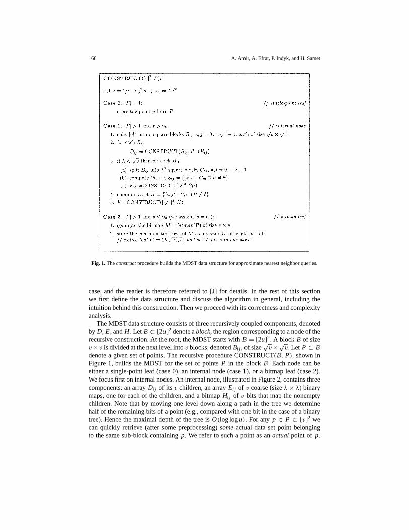
Fig. 1.Theconstructprocedure builds the MDST data structure for approximate nearest neighbor queries.

case, and the reader is therefore referred to [J] for details. In the rest of this sectionwe first define the data structure and discuss the algorithm in general, including theintuition behind this construction. Then we proceed with its correctness and complexityanalysis.

The MDST data structure consists of three recursively coupled components, denotedby D, E, andH . Let B ⊂ [2u]2 denote ablock, the region corresponding to a node of therecursive construction. At the root, the MDST starts withB = [2u]2. A block B of sizev×v is divided at the next level intov blocks, denotedBi j , of size

√v×√v. Let P ⊂ B

denote a given set of points. The recursive procedure CONSTRUCT(B, P), shown inFigure 1, builds the MDST for the set of pointsP in the blockB. Each node can beeither a single-point leaf (case 0), an internal node (case 1), or a bitmap leaf (case 2).We focus first on internal nodes. An internal node, illustrated in Figure 2, contains threecomponents: an arrayDi j of its v children, an arrayEi j of v coarse (sizeλ× λ) binarymaps, one for each of the children, and a bitmapHi j of v bits that map the nonemptychildren. Note that by moving one level down along a path in the tree we determinehalf of the remaining bits of a point (e.g., compared with one bit in the case of a binarytree). Hence the maximal depth of the tree isO(log logu). For anyp ∈ P ⊂ [v]2 wecan quickly retrieve (after some preprocessing)someactual data set point belongingto the same sub-block containingp. We refer to such a point as anactual point of p.


Fig. 2. Illustration of the MDST data structure components at the internal node corresponding to a blockB ofsizev × v.

We use the MDST data structure for the construction of each of the three componentsof the node’s data structure. Hence, all three components are recursively coupledtogether.

The bitmap leaf is a leaf small enough to be processed directly by bitmap techniquesthat are described later. Letv0 = λ1/8 denote the minimal size of a block in the tree, whereλ = 1/ε · log2 u. Rather than pursuing the recursive process until it ends with leaves ofsingle points, we also stop the recursive process whenv ≤ v0 and use a bitmap leaf tostore that region. As shown later, this reduces the query complexity byO(log log logu).In practice, however, it may be omitted for code simplification.

During the preprocessing we first randomly translate the data; this is why the rootblock is of size [2u]2 instead of [u]2. We also precompute certain lookup informationused during thesearchprocedure. The information consists of roughlyO(log5/4 u) bitsand can be computed in the same time. The precomputation procedure is as follows.Consider any pointq ∈ [−1/ε ·v0,1/ε ·v0]2 and any integerr such thatBr (q) (a disk ofradiusr centered atq) intersects but does not contain [v0]2. For each such a pairq, r wecompute a binary matrixMr (q) of sizev0× v0. The matrix has 1’s at pointsp such thatd(p,q) ∈ [r, r +1) and 0’s otherwise. Next, we concatenate the rows ofMr (q) forminga bit vectorAr (q). Finally, we concatenateAr (q) for all r ’s into A(q) and create a tablemappingq to A(q).

The procedure for finding an approximate nearest neighbor is described in Figures 3and 4. To avoid rounding details and to simplify the description we assume that boththe input and output points are members of [u]2 rather than [v]2. Each type of node ishandled separately. Again, we focus first on the process in an internal node (case 1).


Fig. 3.The search procedure for approximate nearest neighbor.

In, general there are three possible situations, illustrated in Figure 5. The algorithm firstapplies a (large) circle test, of radius

√v/ε, which in a sense divides the (unknown)

bits of the result into two parts: the upper bits (most significant bits) and the lower bits(least significant bits). If there is no data point within the circle (Figure 5(a)), then itis a lower bound on the distance to the nearest point which, within the approximation

Fig. 4.The Bitmap procedure (case 2, Figure 3).


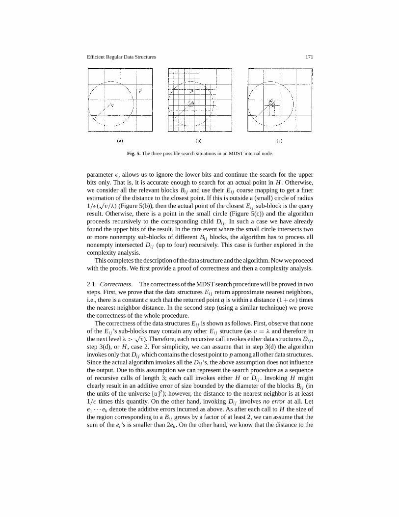
Fig. 5.The three possible search situations in an MDST internal node.

parameterε, allows us to ignore the lower bits and continue the search for the upperbits only. That is, it is accurate enough to search for an actual point inH . Otherwise,we consider all the relevant blocksBi j and use theirEi j coarse mapping to get a finerestimation of the distance to the closest point. If this is outside a (small) circle of radius1/ε(√v/λ) (Figure 5(b)), then the actual point of the closestEi j sub-block is the query

result. Otherwise, there is a point in the small circle (Figure 5(c)) and the algorithmproceeds recursively to the corresponding childDi j . In such a case we have alreadyfound the upper bits of the result. In the rare event where the small circle intersects twoor more nonempty sub-blocks of differentBi j blocks, the algorithm has to process allnonempty intersectedDi j (up to four) recursively. This case is further explored in thecomplexity analysis.

This completes the description of the data structure and the algorithm. Now we proceedwith the proofs. We first provide a proof of correctness and then a complexity analysis.

2.1. Correctness. The correctness of the MDST search procedure will be proved in twosteps. First, we prove that the data structuresEi j return approximate nearest neighbors,i.e., there is a constantc such that the returned pointq is within a distance(1+cε) timesthe nearest neighbor distance. In the second step (using a similar technique) we provethe correctness of the whole procedure.

The correctness of the data structuresEi j is shown as follows. First, observe that noneof the Ei j ’s sub-blocks may contain any otherEi j structure (asv = λ and therefore inthe next levelλ >

√v). Therefore, each recursive call invokes either data structuresDi j ,

step 3(d), orH , case 2. For simplicity, we can assume that in step 3(d) the algorithminvokes only thatDi j which contains the closest point topamong all other data structures.Since the actual algorithm invokes all theDi j ’s, the above assumption does not influencethe output. Due to this assumption we can represent the search procedure as a sequenceof recursive calls of length 3; each call invokes eitherH or Di j . Invoking H mightclearly result in an additive error of size bounded by the diameter of the blocksBi j (inthe units of the universe [u]2); however, the distance to the nearest neighbor is at least1/ε times this quantity. On the other hand, invokingDi j involvesno error at all. Lete1 · · ·ek denote the additive errors incurred as above. As after each call toH the size ofthe region corresponding to aBi j grows by a factor of at least 2, we can assume that thesum of theei ’s is smaller than 2ek. On the other hand, we know that the distance to the


actual nearest neighbor is at least 1/ε · ek. Therefore, the multiplicative error incurred isat most(1+ 2ε).

We can now proceed with the whole data structure. The recursive calls to the algorithmcan be modeled in a similar way to that described above; however, the algorithm hasan additional option of stopping at step 3(c)iii. The latter case can incur an additiveerror bounded by the diameter of the blocksCkl , whereCkl is as defined in Figure 1. Asthe distance to the nearest neighbor is lower-bounded by 1/ε times the side ofCkl , themultiplicative error is at most(1+√2ε). It is easy to verify that the remaining cases areexactly as in the case ofEi j .

In this way we proved the following lemma.

LEMMA 2.1. The distance from p to the point q returned by the algorithm is at most(1+ O(ε)) times the distance from p to its nearest neighbor.

2.2. Complexity. The complexity bounds for the proceduresconstruct, add, anddeleteare essentially as in [vEB]. Therefore, below we focus on the complexity of procedureSEARCH, which follows from the following sequence of claims.

CLAIM 2.2. Case2 of procedureSEARCHtakes time C(ε,u) = d(1/ε)3/8/log1/4 ue.

PROOF. We show that when the whole wordW′ fits within one word, then the procedurecan be implemented in constant time. Otherwise (i.e., whenC(ε,u) = ω(1)), we performthe same procedure sequentially on all words ofW′.

The steps are implemented as follows. Step (a) is performed by multiplyingW bya concatenation ofv bit sequences, each consisting of a 1 followed byv2 − 1 zeros.Step (b) uses just one Boolean operation. The last step can be implemented using aconstant number of Boolean and arithmetic operations as in [FW].

CLAIM 2.3. For any i, j searching in Ei j takes time O((C(ε,u)+ 1/ε) · 1/ε3).

PROOF. Recall that the data structureEi j does not contain otherE-type structures.Therefore, it contains onlyH -type andD-type structures. The recursive structure ofEi j

can be represented as a tree. We observe that the depth of this tree is 3, because by usingthree recursive calls we reduce the block size fromv = λ (the size ofEi j ) to λ1/8 = v0.Searching in any “leaf” data structure (i.e., withv = λ1/8) can be solved in timeC(ε,u).The number of such problems is at most 1/ε3, as the setS′ of data structures invokedrecursively is of size at most 1/ε and the level of recursion is 3. This contributes the firstterm of the cost function, i.e.,C(ε,u)/ε3. The second term follows from the fact thatthe complexity of step 1 is 1/ε2 and this step is invoked at most 1/ε · 1/ε times.

CLAIM 2.4. Consider step3(d) of thesearchalgorithm. If the input P is translated bya random vector, then:

1. The probability that|R| > 1 is at most O((1/ε)/λ).2. The probability that|R| > 2 is most O(((1/ε)/λ)2).


PROOF. We might have|R| > 1 if p lies within distancer ′ of a boundary of some blockBi j (the probability of this event is even smaller as it also requires that the intersectedEi j is not empty). As the side ofBi j is

√v, this event can happen with probability

O(r ′/√v) = O((1/ε)/λ). The other case involvesp lying within distanceO(r ′) from

a vertex of someBi j . The probability of such an event can be estimated in the sameway.

CLAIM 2.5. If for all executions of step3(d), the set R has cardinality at most1,procedureSEARCHruns in O((C(ε,u)+ 1/ε) · log logu · 1/ε4).

PROOF. As each setR has cardinality 1, the recursion path is a path of depth log logu.The cost of each step is dominated by the cost of invokingEi j |S′| = 1/ε times. Thecost estimate follows.

CLAIM 2.6. If for all executions of step3(d), the set R has cardinality at most2,procedureSEARCHruns in time O((C(ε,u)+ 1/ε) · 2log logu · 1/ε4).

PROOF. The argument is similar to the above, but now two recursive calls are allowed.Thus the size of the recursion tree is 2log logu.

CLAIM 2.7. The worst case running time of the search procedure is O((C(ε,u)+1/ε) ·4log logu · 1/ε4).

PROOF. The argument is again similar to the above. In this case, up to four recursivecalls are allowed. This is the (very rare) case in whichp lies within a distancer ′ from avertex of up to four nonemptyBi j blocks.

LEMMA 2.8. The expected running time of thesearchprocedure is O((C(ε,u)+1/ε) ·log logu · 1/ε4).

PROOF. Note that:

• If |R| = 1 for all executions of step 3(d), then the number of times this step is executedis at mostO(log logu).• If |R| ≤ 2 for all executions of step 3(d), then the number of times this step is executed

is at mostO(2log logu) = O(logu).

The expected cost is then on the order of[1 · log logu+

(logu · 1/ε

λ

)logu+

(log2 u ·

(1/ε

λ

)2)

log2 u

](C(ε,u)+1/ε)·1/ε4

which can be verified to be bounded byO((C(ε,u)+ 1/ε) · log logu · 1/ε4).


2.3. Closest Pair Under Insertions. Maintaining the closest pair under insertions canbe reduced to dynamic approximate nearest neighbor (say withε = 1) as follows.First, observe that for anyk, we can retrievek approximate nearest neighbors in timeO(k log logu). To this end, we retrieve one neighbor, temporarily delete it, retrieve thesecond one and so on, untilk points are retrieved. At the end, we add all deleted pointsback to the point set. Next, observe that if we allow point insertions only, then the closestpair distance (call itD) can only decrease with time. The latter happens only if the distanceof the new pointp to its nearest neighbor is smaller thanD. To check if this event hasindeed happened, we retrievek = O(1) approximate nearest neighbors ofp and checktheir distance top. If any of the point’s distances are smaller thanD, we updateD.

To prove the correctness of this procedure, it is sufficient to assume that the distancefrom p to its closest neighbor (sayq) is less thanD. Note that in this case there isat most a constant number of 1-nearest neighbors ofq (as all such points have to liewithin distance 2D of p but have a pairwise distance of at leastD). Therefore, one ofthe retrieved points will be the exact nearest neighbor ofp, and thusD will be updatedcorrectly.

3. Stratified Trees for Higher Dimensions. In this section we present a multidimen-sional variant of stratified trees that solves the approximate nearest neighbor problem intime O(d + log logu + log 1/ε) under the assumption thatd ≤ logn. The data struc-ture is deterministic and static. We first describe a simple variant of the data structurewhich usesdlog loguO(1/ε)dn2 logu storage. We then comment on how to reduce it todlog log loguO(1/ε)dn logu.

The main component of the algorithm is a data structure which finds ad2-approximatenearest neighbor in thel∞ norm. Having a rough approximation of the nearest neighbordistance (call itR), we refine it by using the techniques of [IM] to obtain a(1+ ε)-approximation in the following manner. During the preprocessing, for anyr = 1, (1+ε), (1+ ε)2, . . . (i.e., for O((logu)/ε) different values ofr ) and for each database pointp we build the following data structure, which enables checking (approximately) for aquery pointq if q is within distancer from any database point that lies withinl∞ distanceof O(dr) from p (denote the set of such points byNr (p)). The rough idea of the datastructure is to impose a regular grid of side lengthr/

√d on the space surroundingq

and store each grid cell within distance (approximately)r from Nr (p) in the hash table(see [IM] for details). The data structure usesnO(1/ε)d storage for eachr and p. Thetime needed to perform the query is essentially equal to the time needed to find the gridcell containing the query pointq and compute the value of the hash function appliedto the sequence of all coordinates of that cell. In order to bound this time, notice thatafter finding thed2-approximate nearest neighbor ofq we can (in timed) representq’s coordinates using logd/ε bits per coordinate. Therefore, all coordinates ofq canbe represented usingO(d logd/ε) bits. Since we are allowed to perform arithmeticoperations on words consisting ofd ≤ logu bits in constant time, it is easy to implementthe hashing procedure usingO(logd/ε) operations.

In order to find a(1+ε)-approximate nearest neighbor ofq, we perform a binary searchon log1+ε d values ofr as described in [IM]. This takesO(log(logd)/ε) · O(logd/ε)operations, which is negligible compared withO(d).


Therefore, it is sufficient to find ad2-approximate neighbor ofq quickly. In orderto do this, we apply a variant of the multidimensional stratified trees described in theprevious section. Since the techniques are similar, we only give a sketch. The idea isto split the universe into squares of sided

√u (instead of

√u), as long asd2 <

√u.

Moreover, instead of using only one square grid as before, we used of them, such thatthe i th grid is obtained from the first one by translating it by vector(i

√u, . . . , i

√u).

The reason for this is that for any pointq there is at least onei such that the distancefrom q to the boundary of the cell it belongs to is at least

√u/2. Thus the correctness

argument of the previous section follows. Also, notice that the depth of the data structuredoes not change, as in each step the universe size goes down by a factor of

√u/d > u1/4.

However, the storage requirements are now multiplied bydlog logu, since at each level wemultiply the storage byO(d).

In order to bound the running time, we observe that during each recursive step thevalue of logu is reduced by a constant factor. Therefore, the description size ofq (whichis initially d logu bits long) is reduced by a constant factor (sayc) as well, which means(by the above arguments) that thei th step takes roughlyO(d/ci ) operations, as long asd > ci . Thus, the total time isO(d + log logu).

In order to reduce the storage overhead fromdlog logu to dlog log logu, notice that theabove analysis contains some slack; the time needed for the rough approximation ismuch greater than the time needed for the refinement. One can observe, however, that ifduring the refinement step each coordinate can be represented using logu/log logu bits,its running time is stillO(d). Therefore, we can stop the first phase as soon as the log ofthe universe size drops below logu/log logu, i.e., after the first log log logu steps.

The dependence of the storage size onn can be reduced to linear by using the coveringtechnique of [IM]. More specifically, we can merge those neighborhoodsNr (p) whichhave very large overlap in such a way that the total size of all neighborhoods is only linearand the diameter of the merged neighborhoods gets multiplied by at mostO(logn).

4. Quadtree Dilation in Linear Time. Given a shapeS stored as a region quadtree,T = T(S) as in Section 5.1, we present an algorithm for computing the dilated regionD(S) in O(n) time. The algorithm consists of two major parts. First, it dilates blocks ofa certain size, calledatom blocks, and then it merges the results in a depth-first search(DFS), bottom-up fashion. During the merging process, the algorithm computes andreports the vertices of∂D(S). Each of these parts consists of several steps which arebriefly described below.

We use the following notation: LetR(T) denote the axis-parallel bounding square ofthe region occupied byT . For a nodev of T , let Tv denote the subtree rooted atv, andlet Rv = R(Tv). Sometimes we refer tov (and its regionRv) as theblockv. We say thatv is a gray blockif Rv contains both white (i.e., empty) and black (i.e., full) regions.Let d denote a direction,d ∈ {up,down, left, right}, let edown denote the lower edge10

of R, and letx0 be a point onedown. Let `x0 denote the vertical line passing throughx0. We define theenvelope pointof S with respect toR at x0 in the down direction,

10 The same applies to all other three directions.


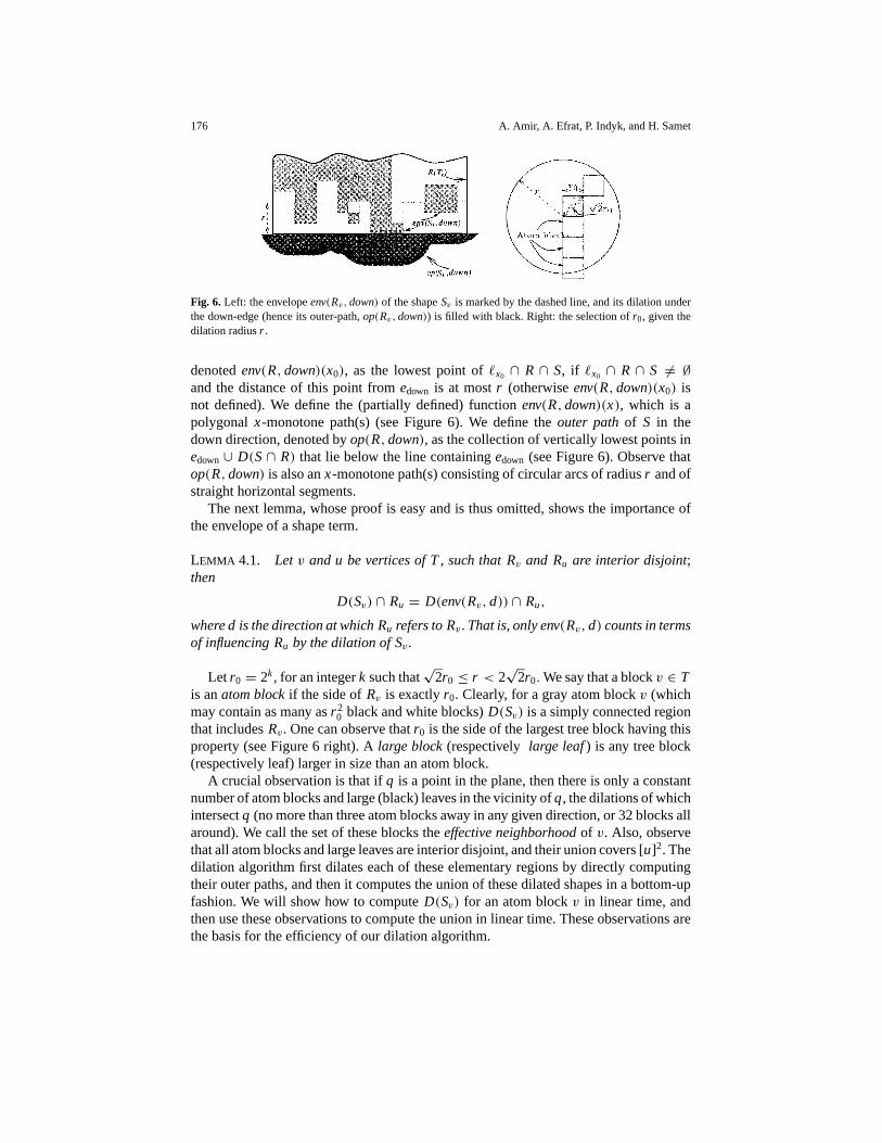
Fig. 6. Left: the envelopeenv(Rv,down) of the shapeSv is marked by the dashed line, and its dilation underthe down-edge (hence its outer-path,op(Rv,down)) is filled with black. Right: the selection ofr0, given thedilation radiusr .

denotedenv(R,down)(x0), as the lowest point of x0 ∩ R ∩ S, if `x0 ∩ R ∩ S 6= ∅and the distance of this point fromedown is at mostr (otherwiseenv(R,down)(x0) isnot defined). We define the (partially defined) functionenv(R,down)(x), which is apolygonal x-monotone path(s) (see Figure 6). We define theouter pathof S in thedown direction, denoted byop(R,down), as the collection of vertically lowest points inedown∪ D(S∩ R) that lie below the line containingedown (see Figure 6). Observe thatop(R,down) is also anx-monotone path(s) consisting of circular arcs of radiusr and ofstraight horizontal segments.

The next lemma, whose proof is easy and is thus omitted, shows the importance ofthe envelope of a shape term.

LEMMA 4.1. Let v and u be vertices of T, such that Rv and Ru are interior disjoint;then

D(Sv) ∩ Ru = D(env(Rv,d)) ∩ Ru,

where d is the direction at which Ru refers to Rv. That is, only env(Rv,d) counts in termsof influencing Ru by the dilation of Sv.

Let r0 = 2k, for an integerk such that√

2r0 ≤ r < 2√

2r0.We say that a blockv ∈ Tis anatom blockif the side ofRv is exactlyr0. Clearly, for a gray atom blockv (whichmay contain as many asr 2

0 black and white blocks)D(Sv) is a simply connected regionthat includesRv. One can observe thatr0 is the side of the largest tree block having thisproperty (see Figure 6 right). Alarge block(respectively large leaf) is any tree block(respectively leaf) larger in size than an atom block.

A crucial observation is that ifq is a point in the plane, then there is only a constantnumber of atom blocks and large (black) leaves in the vicinity ofq, the dilations of whichintersectq (no more than three atom blocks away in any given direction, or 32 blocks allaround). We call the set of these blocks theeffective neighborhoodof v. Also, observethat all atom blocks and large leaves are interior disjoint, and their union covers [u]2. Thedilation algorithm first dilates each of these elementary regions by directly computingtheir outer paths, and then it computes the union of these dilated shapes in a bottom-upfashion. We will show how to computeD(Sv) for an atom blockv in linear time, andthen use these observations to compute the union in linear time. These observations arethe basis for the efficiency of our dilation algorithm.


Computing the Dilation of an Atom Block. The dilation of a gray atom block (ofsize r0 × r0) is a simply connected region, and it can be represented by one list ofthe arcs and straight lines along its boundary, which is a concatenation of the fourouter paths ofv in the four directions. By Lemma 4.1, the outer path in directiond ∈{up,down, left, right} can be computed from the envelopeenv(Rv,d). Hence the dilationof the atom block requires the computation of its four envelopes and then its four outerpaths.

To computeenv(Rv,down) we need to find the partition ofIv = edown(Rv) intointervals, to compute they-location associated with each interval and to construct theenvelope as a list. This is done in two steps. First, we projectTv, the sub-quadtree rootedat v, into a binary tree,T ′v . Then we traverse the binary tree and compute the segmentsand they-location of each segment. Let the nodew′ ∈ T ′v denote the projection of anodew ∈ Tv. The path fromv′ tow′ in T ′v is derived from the path fromv tow in Tv byfollowing the horizontal branches (and ignoring the vertical ones) along the path intv.An example for a region quadtree and its projected binary tree in the down direction isshown on the left of Figure 7.

The procedure PROJECT(Tv) traversesTv in a DFS order, and simultaneously con-structs and traversesT ′v . This is called aprojection, as all the nodesvi ∈ Tv having(1) the same depth (in the quadtree), and (2) the same supportingx-interval, Ivi = Iw′ ,are projected to a single nodew′ ∈ T ′v , associated with this interval (e.g., the three smallblocks which lie along one column in Figure 7 are projected to a single node which isa leaf in this example). During the projection process, each nodew′ ∈ T ′v maintains itsymin(w

′)—the smallesty value of the down-edge of all the black leaves projected to it,if any; otherwise,ymin(w

′) = ∞.

Fig. 7.Left: An atom block and its down-projection binary tree. Right: The projection algorithm.


The envelope is found in the second step by traversingT ′v in a DFS order. The partitionof Iv into envelope segments is just the list ofx-intervals associated with the leaves. They location for an intervalIw′ , however, is not necessarily equal toymin(w

′). It is computedrecursively during this DFS traversal ofT ′v as the smallestymin among all the nodes alongthe path from the rootv′ down to the leafw′. For example, refer to the envelope segment(the thick line) aty = 4, and notice that its leftmost part corresponds to a leaf that carriesymin = 12. The time and space required for the construction ofT ′v and its traversal islinear,O(nv), wherenv is the size ofTv.

The next lemma shows that the result of this process is indeed the envelope. Letpath(T ′v, w

′) = {v1 = v′, v2, . . . , vk = w′} denote the path inT ′v from the rootv′ to anodew′ ∈ T ′v . Let ymin(path(T ′v, w

′)) = min{ymin(v′i ): i = 1, . . . , k} denote the minimal

value ofymin(v′i ) that is encountered alongpath(T ′v, w

′).

LEMMA 4.2. Let x0 ∈ u, and assume x0 ∈ Iw′ wherew′ is a leaf of T′v . Then

env(Rv,down)(x0) = ymin(path(T ′v, w′)).

PROOF. Letw1 ∈ Tv be the black leaf (if any) inTv which intersects the vertical linex = x0 at the lowesty value, y0 = ymin(w1). That is,x0 ∈ Iw1 and, by definition,y0 = env(Rv,down)(x0). Let w′1 ∈ T ′v denote the projection ofw1. It follows thatIw′ ⊆ Iw′1 (w′ is a leaf inT ′v) andw′1 ∈ path(T ′v, w

′). Henceymin(path(T ′v, w′)) ≤

ymin(w′1) ≤ ymin(w1) = y0. The selection ofw1 ensures that there is no lower black leaf

on the path, that is,ymin(path(T ′v, w′)) ≥ ymin(w1) = y0. If there is no such black leaf

w1 ∈ Tv, thenymin(v′i ) = ∞,∀v′i ∈ path(T ′v, w

′).

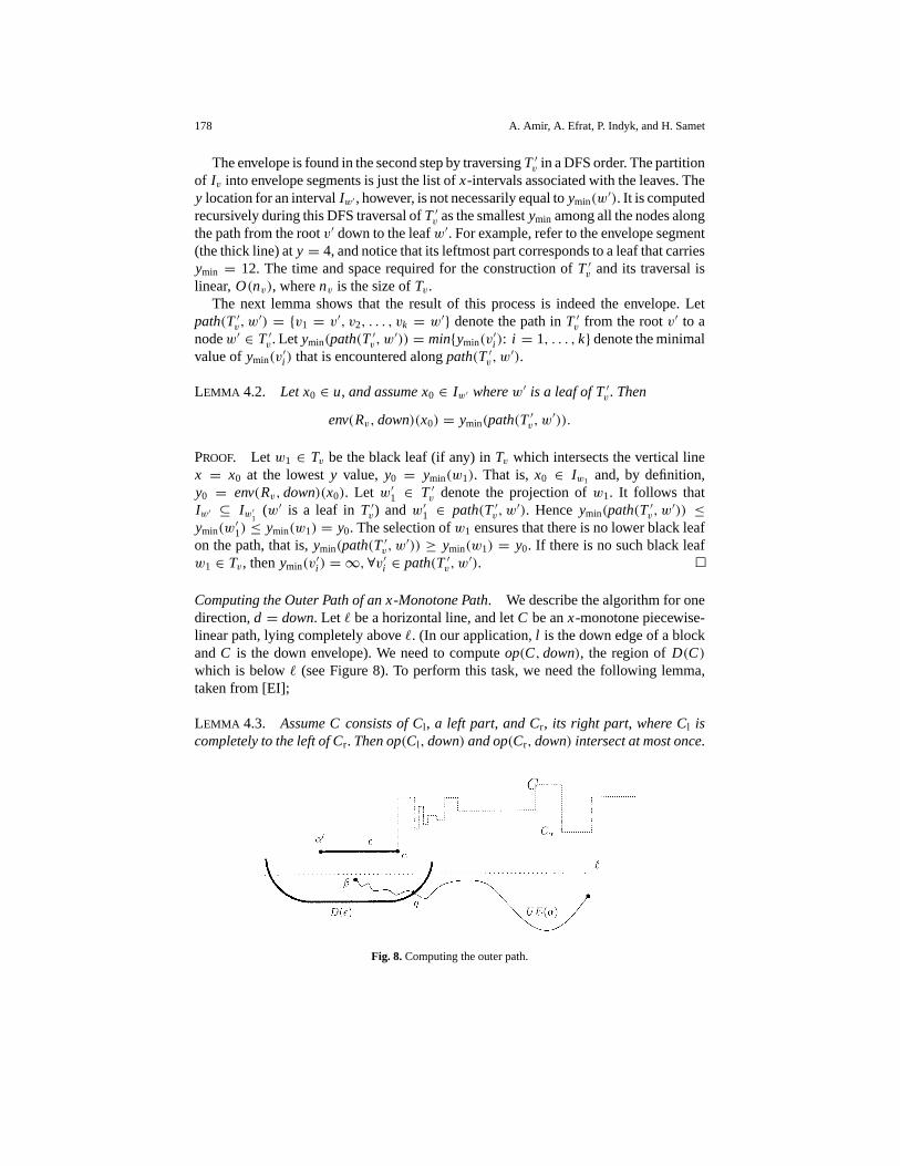
Computing the Outer Path of an x-Monotone Path. We describe the algorithm for onedirection,d = down. Let ` be a horizontal line, and letC be anx-monotone piecewise-linear path, lying completely above. (In our application,l is the down edge of a blockandC is the down envelope). We need to computeop(C,down), the region ofD(C)which is below` (see Figure 8). To perform this task, we need the following lemma,taken from [EI];

LEMMA 4.3. Assume C consists of Cl , a left part, and Cr, its right part, where Cl iscompletely to the left of Cr. Then op(Cl,down) and op(Cr,down) intersect at most once.

Fig. 8.Computing the outer path.


We scanC from right to left, and process one segmente of C at a time. Each suchsegment is a constant-y piece. Letα, α′ denote the right and left points of the currentsegmente, respectively. LetCα denote the part ofC which is to the right ofα. Letopd(α)denoteop(env(Cα,down)). Assume that we have already computedopd(α), and letβ bethe leftmost point ofopd(α). We seekopd(α′). For this, we only need to find the inter-section pointq (if it exists) ofopd(α) and the region ofD(e) below`. Next, we removethe part ofopd(α) lying betweenq andβ, and concatenate the “new” region ofopd(α′)which lies betweenq and the leftmost point ofop(e, R,down) (the outer path ofe).

Finding and deleting the partqβ from opd(α) is achieved as follows: We traverseopd(α) right, starting fromβ, as long as we are inD(e). q is the point at which we leaveD(e). Lemma 4.3 ensures that no other intersection point exists. The time needed forcomputingopd(α′) (afteropd(α) has been determined) is proportional to the complexityof the deleted portionqβ. Since each part in the region is created only once, and canbe removed only once, and since the number of elements inopd(α) is proportional tothe complexity ofC (by [KLPS] cited above) the execution time over the course of theprocedure is linear in the complexity ofC.

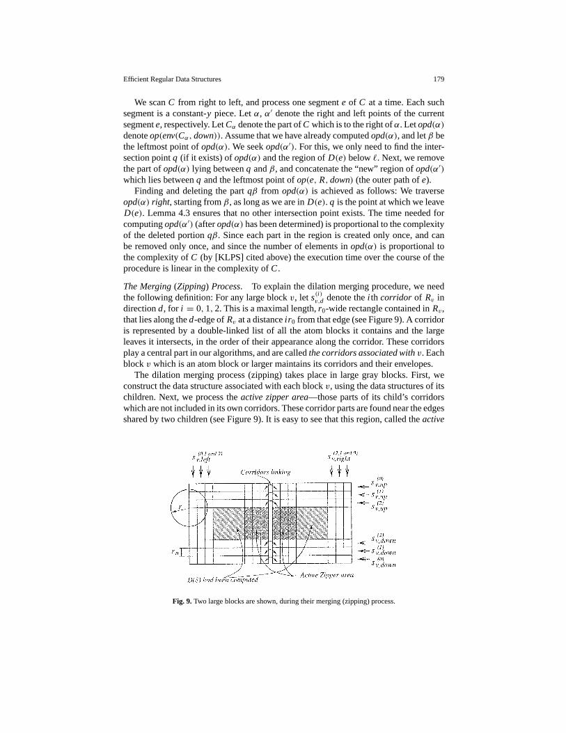
The Merging(Zipping) Process. To explain the dilation merging procedure, we needthe following definition: For any large blockv, let s(i )v,d denote thei th corridor of Rv indirectiond, for i = 0,1,2. This is a maximal length,r0-wide rectangle contained inRv,that lies along thed-edge ofRv at a distanceir 0 from that edge (see Figure 9). A corridoris represented by a double-linked list of all the atom blocks it contains and the largeleaves it intersects, in the order of their appearance along the corridor. These corridorsplay a central part in our algorithms, and are calledthe corridors associated withv. Eachblockv which is an atom block or larger maintains its corridors and their envelopes.

The dilation merging process (zipping) takes place in large gray blocks. First, weconstruct the data structure associated with each blockv, using the data structures of itschildren. Next, we process theactive zipper area—those parts of its child’s corridorswhich are not included in its own corridors. These corridor parts are found near the edgesshared by two children (see Figure 9). It is easy to see that this region, called theactive

Fig. 9.Two large blocks are shown, during their merging (zipping) process.


(or the zipper) region in the figure, is disjoint from the dilated area of any part ofSwhichis outsideRv. Moreover, all the effective neighborhood of this area is either in corridorsor in interior regions (for whichD(S) has already been computed).

The main invariant of the algorithm is the following: When the algorithm exits avertexv toward its parent, all vertices ofD(Sv) whose distance to the boundary ofRvis at least 3r0 have already been reported (see Figure 9). More precisely, before leavingv we compute the vertices ofD(Sv) which lie in those parts of the corridors of its fourchildren that do not intersect with its own corridors (note thatv’s corridors are a subsetof the union of its children’s corridors). It also updates relevant data structures requiredfor further steps of the algorithm. This process is calledmergingor zippingof blocks.

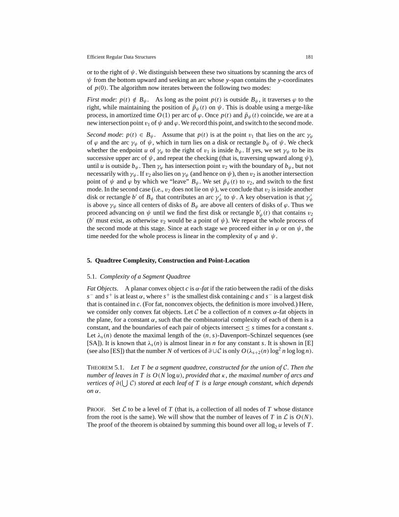
Next, we explain how to compute all the intersections between two outer pathsϕ andψ . We later extract from the results the vertices ofD(S).

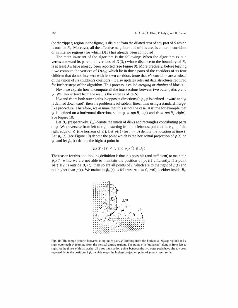
If ϕ andψ are both outer paths in opposite directions (e.g.,ϕ is defined upward andψis defined downward), then the problem is solvable in linear time using a standard merge-like procedure. Therefore, we assume that this is not the case. Assume for example thatψ is defined on a horizontal direction, so letϕ = op(R1,up) andψ = op(R2, right).See Figure 10.

Let Bψ (respectivelyBϕ) denote the union of disks and rectangles contributing partstoψ . We traverseϕ from left to right, starting from the leftmost point to the right of theright edge ofψ (the horizon ofψ). Let p(t) (for t > 0) denote the location at timet .Let pψ(t) (see Figure 10) denote the point which is the horizontal projection ofp(t) onψ , and letpψ(t) denote the highest point in

{pψ(t ′) | t ′ ≤ t, and pψ(t′) /∈ Bψ }.

The reason for this odd-looking definition is that it is possible (and sufficient) to maintainpψ(t), while we are not able to maintain the position ofpψ(t) efficiently. If a pointp(t) ∈ ϕ is outsideBψ(t), then so are all points ofϕ which are to the right ofp(t) andnot higher thanp(t). We maintainpψ(t) as follows. Att = 0, p(0) is either insideBψ

Fig. 10. The merge process between an up outer path,ϕ (coming from the horizontal zigzag region) and aright outer pathψ (coming from the vertical zigzag region). The pointp(t) “traverses” alongϕ from left toright. At the timet of this snapshot all three intersection points between the two outer paths have already beenreported. Note the position ofpψ , which keeps the highest projection point ofp onψ seen so far.


or to the right ofψ . We distinguish between these two situations by scanning the arcs ofψ from the bottom upward and seeking an arc whosey-span contains they-coordinatesof p(0). The algorithm now iterates between the following two modes:

First mode: p(t) /∈ Bψ . As long as the pointp(t) is outsideBψ , it traversesϕ to theright, while maintaining the position ofpψ(t) onψ . This is doable using a merge-likeprocess, in amortized timeO(1) per arc ofϕ. Oncep(t) and pψ(t) coincide, we are at anew intersection pointv1 ofψ andϕ. We record this point, and switch to the second mode.

Second mode: p(t) ∈ Bψ . Assume thatp(t) is at the pointv1 that lies on the arcγϕof ϕ and the arcγψ of ψ , which in turn lies on a disk or rectanglebψ of ψ . We checkwhether the endpointu of γϕ to the right ofv1 is insidebψ . If yes, we setγψ to be itssuccessive upper arc ofψ , and repeat the checking (that is, traversing upward alongψ),until u is outsidebψ . Thenγϕ has intersection pointv2 with the boundary ofbψ , but notnecessarily withγψ . If v2 also lies onγψ (and hence onψ), thenv2 is another intersectionpoint ofψ andϕ by which we “leave”Bψ . We setpψ(t) to v2, and switch to the firstmode. In the second case (i.e.,v2 does not lie onψ), we conclude thatv2 is inside anotherdisk or rectangleb′ of Bψ that contributes an arcγ ′ψ toψ . A key observation is thatγ ′ψis aboveγψ since all centers of disks ofBψ are above all centers of disks ofϕ. Thus weproceed advancing onψ until we find the first disk or rectangleb′ψ(t) that containsv2

(b′ must exist, as otherwisev2 would be a point ofψ). We repeat the whole process ofthe second mode at this stage. Since at each stage we proceed either inϕ or onψ , thetime needed for the whole process is linear in the complexity ofϕ andψ .

5. Quadtree Complexity, Construction and Point-Location

5.1. Complexity of a Segment Quadtree

Fat Objects. A planar convex objectc isα-fat if the ratio between the radii of the diskss− ands+ is at leastα, wheres+ is the smallest disk containingc ands− is a largest diskthat is contained inc. (For fat, nonconvex objects, the definition is more involved.) Here,we consider only convex fat objects. LetC be a collection ofn convexα-fat objects inthe plane, for a constantα, such that the combinatorial complexity of each of them is aconstant, and the boundaries of each pair of objects intersect≤ s times for a constants.Let λs(n) denote the maximal length of the(n, s)-Davenport–Schinzel sequences (see[SA]). It is known thatλs(n) is almost linear inn for any constants. It is shown in [E](see also [ES]) that the numberN of vertices of∂∪C is only O(λs+2(n) log2 n log logn).

THEOREM5.1. Let T be a segment quadtree, constructed for the union ofC. Then thenumber of leaves in T is O(N logu), provided thatκ, the maximal number of arcs andvertices of∂(

⋃C) stored at each leaf of T is a large enough constant, which depends

onα.

PROOF. SetL to be a level ofT (that is, a collection of all nodes ofT whose distancefrom the root is the same). We will show that the number of leaves ofT in L is O(N).The proof of the theorem is obtained by summing this bound over all log2 u levels ofT .


Let v be a leaf node ofL. The complexity ofRparent(v) ∩ ∂⋃C is larger thanκ

(otherwiseparent(v) would have been a leaf). LetR be a square whose center coincideswith the center ofRv, and whose edge-length is larger by some factorκ ′ > 1 than theedge-length ofR, whereκ ′ > 1 depends onα. Using arguments similar to the ones usedin [EKNS], we can show that at least one of the following cases must occur:

• There is an objectc ∈ C such thatR containsz, a rightmost, a leftmost, a highest or alowest point of∂c.• R contains a vertexz of ∂

⋃C.

• There is an objectc ∈ C such that the area ofR∩ c is at least a constant fraction ofthe area ofc.

In the first two cases, the pointz can be charged for at mostκ ′ blocksv. Similarly, in thethird case, we charge the region ofc. Since the number of verticesz of ∂

⋃C is O(N)

and the number of elements that we charge in the first and third cases isO(n) = O(N),we conclude that the number of leaf-nodesv in L is O(N), as asserted.

Let T = T(S) denote a (region) quadtree representing a shapeS, and letNl denotethe number of leaves inT . It is known that sinceS consists of≤ Nl disjoint convexobjects, namely the black blocks, then∂D(S) containsO(Nl ) vertices (see [KLPS]).Combining this bound with the fact that the dilation of a black block ofT is always a fatregion, we can prove the following lemma, using exactly the same argument as in theproof of Theorem 5.1.

LEMMA 5.2. Let T be a segment quadtree constructed for∂D(S). Then the number ofleaves inT is O(Nl logu).

REMARK. Recall that the number of nodes in a compressed (respectively uncom-pressed) quadtree is at most two (respectively logu) times the number of leaves.

5.2. Constructing Quadtrees

Storing D(S). The above discussion shows thatD(S) can be efficiently stored in aquadtree. In Section 4 we showed howD(S) can be computed in (optimal) linear time.We later employ this algorithm in order to store the result in a convenient form, e.g., asegment quadtree (this requires only a slightly higher complexity).

In this section we show that it is convenient to store the output of the dilation algorithmof Section 4 as a segment quadtree.

THEOREM5.3. Let S be a planar shape given as a region quadtree T, consisting of nnodes, and let r be a given radius. We can construct a segment quadtreeT that storesD(S) in time and space O(n log2 u).

PROOF. The constructive proof requires the following definitions (see [dBvKOS]): Abalancedquadtree is a quadtree with the additional property that ifv1 andv2 are nodes inthe tree such thatRv1 andRv2 share an edge or a portion of an edge, then the depth ofv1

differs by at most 1 from the depth ofv2. A quadtree of sizen can be balanced by adding


O(n) additional nodes [dBvKOS, Theorem 14.4]. Anettedquadtree is a quadtree whereif Rv1 andRv2 are neighboring squares, then there exists a pointer, called anet pointer,from v1 to v2 and fromv2 to v1 [S1]. The combination of both attributes guarantees thatonly a constant number of net pointers are attached to each node.

We can now describe the algorithm. We start with an empty output treeT . We maintainT as both netted and balanced, and all its nodes are stored in a hash tableH . We run thedilation algorithm of Section 4, whose output can be arranged (that is, directly reported)as a collection of closed curves of∂D(S). The output quadtree is built in two phases.

First, we perform the following procedure for each of the closed curves. LetC besuch a curve. We pick an arbitrary pointq of C, and find the leaf cellv of T containingq, usingH , by the point-location data structure of Section 5.3. We insert the arcs ofCinto v, in the order they appear alongC. If at some point the number of arcs inv exceedsthe thresholdκ of T , we splitv, and accordingly update the hash table, the net pointers,and perhaps split node(s) in order to keep the tree balanced (which may require furthersplits, but, as stated above, it requires only a linear number of additional nodes). If, onthe other hand, the arcγ of C we follow intersects the boundary ofRv and “leaves” thisblock, then we use the net pointers to find the neighbor leaf into whichγ “enters,” andcontinue the process in that block. As noted, each node has only a constant number ofneighbors to keep track of.

Next, we have to scan the empty block (that does not intersect∂D(S)) and labeleach such block as to whether it is fully inside or outsideD(S). This is done using analgorithm similar to the connected component labeling algorithm [S1]. We traverse thetree, while adding all the nonempty leaves to a queue. Next, we pop one leaf at a time,use it to label its (yet unlabeled) empty neighbors, and add only those newly labelednodes to the queue.

When bounding the running time of this algorithm, it is clear that phase two takes onlylinear time. For phase one, we first have to calculate the time needed to perform all thesingle point-location operations, one per boundary path ofD(S). Their number cannotexceedO(n) (and is assuredly much smaller). Using the technique from Theorem 5.5,each one takesO(log logu) time, or a total ofO(n log logu). The remaining runningtime is proportional (since no vertex is ever deleted) to the number of nodes created inT , which we denote bym. By Lemma 5.2 we know thatm = O(n log2 u) and thus wehave proved Theorem 5.3.

The size of the resulting quadtree can be improved by a factor of logu/log logn byusing the compressed quadtree (as in this case the tree size is proportional to the numberof leaves). The following lemma shows that in this case the running time is improved byalmost the same factor.

LEMMA 5.4. Given ninterior disjointobjects, a compressed quadtree representatationof their union can be computed in time O(N log logu),where N is the size of the resultingquadtree.

PROOF. The idea is similar to the algorithm described above. The difference is that nowwe need to perform the point location inO(log logu) time in a compressed tree, insteadof O(logu) time as before. Also, the time needed to jump between neighboring leaves is


no longer constant, as we cannot afford to maintain a balanced tree. Thus, we will haveto make sure that this operation can be done inO(log logu) time as well. We use thecorresponding technique from Theorem 5.5, i.e., hashO(log logu) paths per tree edgeto achieveO(log logu) query time. The total time spent on updating the hash tables isO(N log logu), which is within the bounds.

The last point we have to verify is that while constructing the output quadtree wedo not generate long paths which should be replaced by single edges in the compressedquadtree. This can be easily done by applying unbounded binary search.

By applying the technique from the above lemma to Theorem 5.3, we obtain analgorithm for computing a compressed quadtree of the dilated shape inO(N ′ log logu)time, whereN ′ is the size of the quadtree.

Finally, we address the problem of point location in quadtrees. First we considerqueries in arbitrary quadtrees and compressed quadtrees. Then we consider queries inquadtrees of dilated shapes. In the latter we show that in order to answer such queriesefficiently we do not even need to calculate the dilated shape.

5.3. A Point-Location Data Structure

THEOREM5.5. Let S be a planar shape consisting of a union of cells of the integer grid[u]2, and given as an uncompressed quadtree T, consisting of n nodes. Then in timeO(n) we can construct a data structure of size O(n), such that given an integer querypoint q, we can determine whether q lies inside S in(expected) time O(log logu). If Tis a compressed quadtree, then we can construct the data structure in time and spaceO(n log logu) and expected query time O(log logu).

PROOF. Consider first the case in whichT is an uncompressed quadtree. We store thenodes ofT in a hash table. The key of each nodev is the binary representation of thepath from the root ofT to v, which is merely the position in [u]2 of the blockv. Given aquery point, we perform binary search on the height of the tree to find the leaf level. Ateach level probed we check if there is a node ofT at that level (which lies on the pathleading to the leaf includingq). We can find the leaf containingq, or determine that nosuch block exists, in expected timeO(log logu). This idea has appeared in the literature[W].

When T is a compressed tree, the analysis is a bit more complicated. This is dueto the fact that simple replication of the previous approach would seemingly requirehashing all the paths in the tree, which would imply anO(nt) storage requirement,wheret = O(logu) is the depth of the tree. However, the following observation allowsus to reduce the storage toO(n log logu). Call an interval{i · · · j } ⊂ [t ] a primitiveinterval if i = k2p and j = (k+ 1)2p for somek andp. Each such interval correspondsto a subtree of a binary tree decomposition of [t ]. Thus [t ] can be decomposed intoprimitive intervals in a tree-like fashion, by finding the largest primitive intervalJ in [t ],removingJ from [t ], and recursing on [t ]\J. One can observe that such a decompositionis unique, and [t ] is decomposed intoO(log2 t) primitive intervals, since for everyp, atmost one primitive interval of length 2p can appear in the decomposition.


The algorithm proceeds as follows. Each compressed edge is split intoO(log t)primitive intervals. Instead of hashing all paths, the algorithm hashes only the paths withendpoints at primitive intervals. The following claim, whose proof is straightforward andomitted, shows that this restriction does not influence the behavior of the binary searchprocedure, and thus concludes the proof of Theorem 5.5.

CLAIM 5.6. Let e be a compressed edge in the quadtree from level i to level j> i andlet l be any level probed during the binary search for any point q. Then l has to be anendpoint of one of O(log( j − i + 1)) primitive intervals from the decomposition of theinterval [i · · · j ].

5.4. Point Location in Dilated Shape. We address the problem of point location in thedilation of a given shape. We show that in order to answer such queries efficiently wedo not even need to calculate the dilated shape.

THEOREM5.7. Let S be a planar shape given as a region quadtree T consisting of nnodes defined on the integer grid[u]2, and let r be a given radius. Then in time O(n)we can construct a data structure of size O(n), such that given an integer query pointq, we can determine whether q lies inside D(S) in expected time O(log logu).

PROOF. The data structure consists of two parts. The first part enables us to find whetherq lies in S itself, for which we use the data structure of Theorem 5.5. If the query pointis not in S, then we need to check if it falls in the dilated region, which is the goal ofthe second part of the data structure. The construction of the second part takes placeduring the execution of the dilation algorithm of Section 4. Let0 be a grid imposedon [u]2 such that each point of0 corresponds to an atom block of sider0. Thus everyatom block has a unique identifier—a pair of integers representing its location in0.Similarly, we give a unique identifier to each corridor we encounter during the dilationalgorithm. All these identifiers are stored in a hash table. Thus for any query pointq,we can find each atom block which containsq (and at most three blocks in its vicinityvertically above and belowq) and accordingly access the data structure associated withthis corridor.

The additional data structure associated with a corridors is as follows. Assumes isvertical. We describe a data structure foropleft, the outer path coming intos from theregion ofS that lies to the right ofs. The structure for the outer paths emerging fromother three directions is analogous. To conclude the construction of the data structure, wesweep the vertices ofopleft, and truncate the coordinates of their vertices to integers, thusunifying sequences of vertices whose integer truncated value is the same into a singlevertex. Next, we assign to each vertexu the arcs ofopleft adjacent tou, and constructa van Emde Boas tree for they-coordinate of the vertices ofopleft. The constructiontime is O(k), wherek is the number of vertices onopleft. By performing a query to thatdata structure (in timeO(log logu)) we find the objects (disks and rectangles) whoseboundaries form the arcs associated withw, and thus determine if one of them containsq. Similar data structures are constructed for the upper and lower outer paths of eachof the atom blocks, which allows us to perform similar queries on the blocks above and


belowq. Clearly if a disk or a rectangle of the dilated area containsq, we will find it inthis way.

6. Discussion. This paper provides optimal and near-optimal algorithms for severalproblems in computational geometry on the integer grid. We show that under the as-sumption that the input points have limited precision (i.e., are drawn from the integergrid of sizeu) these data structures yield efficient solutions to many important prob-lems. In many cases we are able to replaceO(logn) with O(log logu). This requires anefficient evaluation of the logu bits required to write the result. We solve this problemusing regular data structures. Some of these regular data structures, like the quadtree,can be stored in hash tables, which allow us to process, for example, a point locationquery without having to traverse the whole path from the root to the leaf (which wouldtakeO(logu)). In other cases, as with the MDST, the regular data structure divides thelocation bits at each recursive level into two significantly large parts, and therefore theheight of the tree becomes log logu. Most of these algorithmic problems otherwise haveÄ(logn) lower bounds in a standard algebraic tree model, assuming arbitrary precisioninput. These basic ideas can be used to improve the efficiency of many other algorithms.

In several of the algorithms we stop the recursion process before it reaches the trivialtype of leaf, and handle the rather complex “leaf” using a separate, nonrecursive algo-rithm. For example, in the quadtree dilation algorithm, if we try to eliminate the notion ofan atom block, and just apply the dilation and merge starting directly from the quadtreeleaves, the complexity will no longer be linear and independent ofR. In order to achievethe desired efficiency we must identify the level at which the recursion process must bestopped and replaced with a nonrecursive algorithm.

In some situations, the random translation in the MDST algorithm and the correspond-ing expected complexity bounds are undesired. In such a case, the problem that occursnear the borders betweenBi j blocks can be transferred from the query time to the updatetime. If one extends the borders of theBi j blocks to have them overlap in a 2r ′-wideregion, then there will always be a block that contains the entire small circle around thequery pointq (see Figure 5(c)). Therefore, there is no need to recurse into more thanone child (i.e.,|R| = 1 at all times). This requires, however, some modification of theinsert and delete procedures, which in turn should allow insertion/deletion of a pointinto/from all the blocks it intersects with.

References

[AMN+] S. Arya, D. M. Mount, N. S. Netanyahu, R. Silverman, and A. Y. Wu. An optimal algorithmfor approximate nearest neighbor searching. InProc. Fifth Annual ACM–SIAM Symposium onDiscrete Algorithms, pages 573–582, 1994.

[BF] P. Beama and F. Fich. Optimal bounds for the predecessor problem. InProc. 31st ACM Sym-posium on Theory of Computing, pages 295–304, May 1999.

[dBvKOS] M. de Berg, M. van Kreveld, M. Overmars, and O. Schwarzkopf.Computational Geometry:Algorithms and Applications. Springer-Verlag, Berlin, 1997.

[DST] M. B. Dillencourt, H. Samet, and M. Tamminen. A general approach to connected-componentlabeling for arbitrary image representations.Journal of the ACM, 39(2):253–280, April 1992.


[E] A. Efrat. The complexity of the union of(α, β)-covered objects.Proc. 15th Annual ACMSymposium on Computational Geometry, pages 134–142, 1999.

[EI] A. Efrat and A. Itai. Improvements on bottleneck matching and related problems using geometry.In Proc. 12th Annual ACM Symposium on Computational Geometry, pages 301–310, May 1996.

[EKNS] A. Efrat, M. J. Katz, F. Nielsen, and M. Sharir. Dynamic data structures for fat objects and theirapplications. InProc. 5th Workshop on Algorithms and Data Structures, pages 297–396, 1997.

[ES] A. Efrat and M. Sharir. On the complexity of the union of fat objects in the plane. InProc. 13thAnnual ACM Symposium on Computational Geometry, pages 104–112, 1997.

[FW] M. L. Fredman and D. E. Willard. Blasting through the information theoretic barrier with fusiontrees. InProc. 22nd ACM Symposium on Theory of Computing, pages 1–7, 1990.

[IM] P. Indyk and R. Motwani. Approximate nearest neighbors: towards removing the curse ofdimensionality. InProc. 30th ACM Symposium on Theory of Computing, pages 604–613, May1998.

[J] D. B. Johnson. A priority queue in which initialization and queue operations takeO(log(log(D))) time.Mathematical Systems Theory, 15:295–309, 1982.

[KLPS] K. Kedem, R. Livne, J. Pach, and M. Sharir. On the union of Jordan regions and collision-free translational motion amidst polygonal obstacles.Discrete & Computational Geometry,1:59–71, 1986.

[M] H. Muller. Rastered point locations. InProc.Workshop on Graphtheoretic Concepts in ComputerScience, pages 281–293, 1985.

[O] M. H. Overmars. Range searching on a grid.Journal of Algorithms, 9:254–275, 1988.[RGK] J.I. Munro and R. G. Karlsson. Proximity on a grid. InProc. 2nd Symposium on Theoretical

Aspects of Computer Science, pages 187–196, 1985.[S1] H. Samet.Applications of Spatial Data Structures: Computer Graphics, Image Processing, and

GIS. Addison-Wesley, Reading, MA, 1990.[S2] H. Samet.The Design and Analysis of Spatial Data Structures. Addison-Wesley, Reading, MA,

1990.[SA] M. Sharir and P. K. Agarwal.Davenport–Schinzel Sequences and Their Geometric Applications.

Cambridge University Press, New York, 1995.[vEB] P. van Emde Boas. Preserving order in a forest in less than logarithmic time.Information

Processing Letters, 6:80–82, 1977.[W] D. E. Willard. Log-logarithmic worst-case range queries are possible in spaceθ(n). Information

Processing Letters, 17:81–84, 1983.

Algorithmica - UMD

Documents

Transcript of Algorithmica - UMD