BOSTON UNIVERSITY Dissertation
210
BOSTON UNIVERSITY GRADUATE SCHOOL OF ARTS AND SCIENCES Dissertation DETECTOR DEVELOPMENT FOR DIRECTION-SENSITIVE DARK MATTER RESEARCH by HIDEFUMI TOMITA B.S., University of California, San Diego, 2004 Submitted in partial fulfillment of the requirements for the degree of Doctor of Philosophy 2011
Transcript of BOSTON UNIVERSITY Dissertation

BOSTON UNIVERSITY
GRADUATE SCHOOL OF ARTS AND SCIENCES
Dissertation
DETECTOR DEVELOPMENT FOR DIRECTION-SENSITIVE
DARK MATTER RESEARCH
by
HIDEFUMI TOMITA
B.S., University of California, San Diego, 2004
Submitted in partial fulfillment of the
requirements for the degree of
Doctor of Philosophy
2011

Approved by
First ReaderSteven P. Ahlen, Ph.D.University Professor and Professor of Physics
Second ReaderRobert M. Carey, Ph.D.Associate Professor of Physics

Acknowledgments
I would love to thank my parents, Etsuo and Yoshiko, and my sister, Ai, for always be-
lieving in and supporting me in my life journey. Although the life path I have chosen so
far may be the furthest from what a typical Japanese man would pick, you were always
there for me. I could not have accomplished such a big goal without your support. I would
also love to thank Shelby Patton for loving and supporting me for the latter half of my
graduate student career. Since I met you, I have become like a fish who found water. You
taught me the joy of life and, thanks to you, I will always love my life with you.
I would like to thank Lora Brill for all the love and joy we shared together. I was so lucky to
have spent part of my life with you - we grew together, we laughed together, and we cried
together. I would not have been who I am without you. Also my best friend, Alvaro Roc-
caro; it still hurts me when I think of having you lost so young. But, because of you, I can
really appreciate what I have now, and I have enjoyed every single day of my life since then.
Thank you very much to my adviser, Professor Steve Ahlen, for guiding me through my
graduate student career. I was very lucky to have joined your group at a most perfect tim-
ing imaginable. You taught me disciplines and techniques that I will need as a scientist.
Thank you very much to my friend/co-worker, Andrew Inglis, for helping me at work and
being such a great friend. And I would love to thank all my friends - all international and
American - for sharing an amazing time with me in my life.
iii

DETECTOR DEVELOPMENT FOR DIRECTION-SENSITIVE
DARK MATTER RESEARCH
(Order No. )
HIDEFUMI TOMITA
Boston University Graduate School of Arts and Sciences, 2011
Major Professor: Steven P. Ahlen, University Professor and Professor of Physics
ABSTRACT
The existence of Dark Matter was first proposed by Fritz Zwicky in 1933, based on the ob-
served velocity distribution of galaxies in the Coma Cluster. Subsequent studies of visible
mass and velocity distributions in other galaxies have confirmed Zwicky’s original observa-
tion; there is now little doubt that Dark Matter exists. However, due to the fact that Dark
Matter interacts very weakly through non-gravitational forces, nothing is known about the
nature of Dark Matter. It is believed that Dark Matter particles are streaming toward the
Earth, in the Earth’s rest frame, from the direction of the constellation Cygnus. Obser-
vation of this so-called Dark Matter ’wind’ with a direction-sensitive dark matter particle
detector would be compelling evidence that Dark Matter does consist of a gas of discrete
particles as a new form of matter. The DMTPC collaboration is developing such a detector,
and this thesis describes R&D work in support of that project. The DMTPC technique
for looking for Dark Matter relies on Dark Matter particles interacting with atomic nuclei,
causing the nuclei to recoil and to leave optical signals that can be detected. Since neu-
trons are electrically neutral and collide with nuclei, they can mimic Dark Matter signals.
Therefore, the reduction of neutron background is critical to the successful detection and
identification of Dark Matter particles. One important aspect of this thesis is to fully
understand and quantify neutron interactions with our detector. In addition to providing
information for understanding Dark Matter experiments, this work also allows us to under-
iv

stand how our device can be used as a neutron detector. We have been able to measure a
number of neutron events in a variety of experimental runs both with and without neutron
sources such as a neutron generator and 252Cf. From these runs, we have obtained data for
both elastic and inelastic interactions of neutrons of various energy ranges with detector
gas nuclei. In this thesis, I will also discuss our current background data taking for the
Dark Matter research and our plan for scaling up the detector to 100 m3 for a competitive
Dark Matter search.
v

Contents
1 History and Theoretical Motivation of Dark Matter 1
1.1 Historical Background . . . . . . . . . . . . . . . . . . . . . . . . . . . . . . 1
1.2 General Detection Method . . . . . . . . . . . . . . . . . . . . . . . . . . . . 5
1.2.1 Detection Technique . . . . . . . . . . . . . . . . . . . . . . . . . . . 5
1.2.2 Daily/Seasonal Modulation . . . . . . . . . . . . . . . . . . . . . . . 6
1.2.3 Other Capabilities of the Detector . . . . . . . . . . . . . . . . . . . 9
2 DMTPC Detection Method 11
2.1 Fundamental Detector Concept . . . . . . . . . . . . . . . . . . . . . . . . . 11
2.2 CF4 Gas . . . . . . . . . . . . . . . . . . . . . . . . . . . . . . . . . . . . . . 14
2.3 Neutron Detection . . . . . . . . . . . . . . . . . . . . . . . . . . . . . . . . 20
3 DMTPC Detector 23
3.1 Detector Introduction . . . . . . . . . . . . . . . . . . . . . . . . . . . . . . 23
3.2 First R&D Wire Chamber at MIT . . . . . . . . . . . . . . . . . . . . . . . 26
3.3 Prototype Dark Matter Detector at Boston University . . . . . . . . . . . . 32
3.3.1 First Wire Chamber Components . . . . . . . . . . . . . . . . . . . . 32
3.3.2 Improvement to Mesh Chamber . . . . . . . . . . . . . . . . . . . . . 40
3.3.3 EMCCD . . . . . . . . . . . . . . . . . . . . . . . . . . . . . . . . . . 43
3.3.4 Up-To-Date DM Prototype Detector . . . . . . . . . . . . . . . . . . 50
4 Fast-Neutron Tests with Prototype DM Detector at MIT 53
vi

4.1 Fast Neutron Detection from 252Cf . . . . . . . . . . . . . . . . . . . . . . . 53
4.1.1 Introduction to 252Cf Neutron Runs . . . . . . . . . . . . . . . . . . 53
4.1.2 252Cf Run Data with Pure CF4 Gas in BU Prototype . . . . . . . . 55
4.1.3 Electron Diffusion Check in 40 torr CF4 Gas . . . . . . . . . . . . . 59
4.1.4 252Cf Run Data with Gas Mixture of CF4 and 4He in BU Prototype 61
4.1.5 Electron Diffusion Check in Gas Mixture of 40 torr CF4 and 4He . . 62
4.1.6 Directionality Capability of our Detector . . . . . . . . . . . . . . . 62
4.2 Fast Neutron Detection from D+T Neutron Generator at MIT . . . . . . . 69
4.2.1 Introduction to D+T Neutron Generator Neutron Runs . . . . . . . 69
4.2.2 D+T Neutron Generator Run Data with Pure CF4 Gas in BU Pro-
totype . . . . . . . . . . . . . . . . . . . . . . . . . . . . . . . . . . . 71
5 Preliminary TPC Experiment with Xe Gas 79
5.1 Scintillation Characteristics of Xe Gas . . . . . . . . . . . . . . . . . . . . . 79
5.2 Non-Linearity of the Stopping Power of Xe Gas . . . . . . . . . . . . . . . . 83
6 Preparations for the Background Neutron Detection Experiment 87
6.1 EMCCD and PMT Dual Readout System . . . . . . . . . . . . . . . . . . . 87
6.2 Two Experiments for the BU Prototype Chamber Quantification . . . . . . 90
6.2.1 Spark Experiment . . . . . . . . . . . . . . . . . . . . . . . . . . . . 90
6.2.2 Correlation Experiment . . . . . . . . . . . . . . . . . . . . . . . . . 95
6.2.3 Electron Diffusion Effect on EMCCD Readout . . . . . . . . . . . . 100
7 Thermal Neutron Measurement with BU Prototype Chamber 103
7.1 Thermal Neutron Absorption of 3He . . . . . . . . . . . . . . . . . . . . . . 103
7.2 Thermal Neutron Data Measurement . . . . . . . . . . . . . . . . . . . . . . 106
7.3 Thermal Neutron Data Result . . . . . . . . . . . . . . . . . . . . . . . . . . 110
7.4 Determining the 3D Full Track Length . . . . . . . . . . . . . . . . . . . . . 114
7.5 Change of Gas Gain and Energy Threshold . . . . . . . . . . . . . . . . . . 115
vii
7.6 Thermal Neutron Flux . . . . . . . . . . . . . . . . . . . . . . . . . . . . . . 123
8 Cylon: A New Direction-Sensitive Fast Neutron Detector 127
8.1 Introduction to Cylon . . . . . . . . . . . . . . . . . . . . . . . . . . . . . . 127
8.2 Thermal Neutron Capture Event Data with Cylon Detector . . . . . . . . . 140
8.2.1 Electron Drift Velocity . . . . . . . . . . . . . . . . . . . . . . . . . . 140
8.2.2 Gain Variation Problem . . . . . . . . . . . . . . . . . . . . . . . . . 142
8.2.3 Applying Data Correction to Improve the Gain Non-Uniformity . . . 146
8.2.4 Change of Triggering System . . . . . . . . . . . . . . . . . . . . . . 146
8.2.5 Thermal Neutron Flux by Cylon . . . . . . . . . . . . . . . . . . . . 149
8.3 Cosmic Ray Neutron Data with Cylon as a Fast Neutron Detector . . . . . 151
8.3.1 Initial Motivation of Cylon Fast Neutron Detector . . . . . . . . . . 151
8.3.2 Background Cosmic Ray Neutron Data by Cylon . . . . . . . . . . . 156
8.4 Detector Improvements . . . . . . . . . . . . . . . . . . . . . . . . . . . . . 159
8.4.1 Improvement for Active Interrogation . . . . . . . . . . . . . . . . . 159
8.4.2 Improvement for Gas Gain . . . . . . . . . . . . . . . . . . . . . . . 161
9 Dark Matter Background Data Run by Cylon 163
9.1 20-Day Background Data by Cylon with Gas Mixture of 3He . . . . . . . . 163
9.2 Particle Identification in Large Energy or Long Track Region . . . . . . . . 166
9.3 Particle Identification at MeV Region . . . . . . . . . . . . . . . . . . . . . 167
9.4 Particle Identification at Dark Matter Energy Region . . . . . . . . . . . . . 170
9.5 Cosmic Ray Neutron Induced Inelastic Recoils and Summary . . . . . . . . 172
10 Conclusion and Next Goal 177
10.1 Current Status of DMTPC Collaboration . . . . . . . . . . . . . . . . . . . 177
10.2 1 m3 Dark Matter Detector . . . . . . . . . . . . . . . . . . . . . . . . . . . 178
10.2.1 Sensitivity and Limits . . . . . . . . . . . . . . . . . . . . . . . . . . 178
10.2.2 Design . . . . . . . . . . . . . . . . . . . . . . . . . . . . . . . . . . . 180
viii

10.3 100 m3 Dark Matter Detector . . . . . . . . . . . . . . . . . . . . . . . . . . 182
Bibliography 184
Curriculum Vitae 190
ix

List of Figures
1.1 Dark Matter evidence . . . . . . . . . . . . . . . . . . . . . . . . . . . . . . 2
1.2 WMAP data . . . . . . . . . . . . . . . . . . . . . . . . . . . . . . . . . . . 3
1.3 Bullet cluster . . . . . . . . . . . . . . . . . . . . . . . . . . . . . . . . . . . 4
1.4 SD and SI exclusion limits . . . . . . . . . . . . . . . . . . . . . . . . . . . . 6
1.5 Anual modulation . . . . . . . . . . . . . . . . . . . . . . . . . . . . . . . . 7
1.6 DAMA/LIBRA data . . . . . . . . . . . . . . . . . . . . . . . . . . . . . . . 8
1.7 Daily modulation . . . . . . . . . . . . . . . . . . . . . . . . . . . . . . . . . 9
2.1 DMTPC detection method . . . . . . . . . . . . . . . . . . . . . . . . . . . 12
2.2 CF4 scintillation spectrum . . . . . . . . . . . . . . . . . . . . . . . . . . . . 14
2.3 CF4 electron-to-photon ratio . . . . . . . . . . . . . . . . . . . . . . . . . . 15
2.4 Energy loss of a traveling charged particle . . . . . . . . . . . . . . . . . . . 18
2.5 Electron mobility of CF4 gas . . . . . . . . . . . . . . . . . . . . . . . . . . 19
2.6 Electron diffusion experiment setup . . . . . . . . . . . . . . . . . . . . . . . 20
2.7 Electron diffusion experiment result . . . . . . . . . . . . . . . . . . . . . . 21
2.8 High-energy neutron cross section . . . . . . . . . . . . . . . . . . . . . . . . 22
2.9 Thermal neutron cross section . . . . . . . . . . . . . . . . . . . . . . . . . . 22
3.1 . . . . . . . . . . . . . . . . . . . . . . . . . . . . . . . . . . . . . . . . . . . 25
3.2 Data acquisition schematics . . . . . . . . . . . . . . . . . . . . . . . . . . . 26
3.3 First generation R&D chamber . . . . . . . . . . . . . . . . . . . . . . . . . 27
3.4 QE of Kodak KAF-0401 . . . . . . . . . . . . . . . . . . . . . . . . . . . . . 28
x

3.5 First generation TPC setup . . . . . . . . . . . . . . . . . . . . . . . . . . . 29
3.6 First successful image capture of an α particle . . . . . . . . . . . . . . . . . 30
3.7 BU prototype chamber . . . . . . . . . . . . . . . . . . . . . . . . . . . . . . 34
3.8 BU prototype wire frames . . . . . . . . . . . . . . . . . . . . . . . . . . . . 35
3.9 Wire transfer frame from BNL . . . . . . . . . . . . . . . . . . . . . . . . . 35
3.10 BU prototype wire chamber setup . . . . . . . . . . . . . . . . . . . . . . . 36
3.11 QE of Kodak KAF-1603ME . . . . . . . . . . . . . . . . . . . . . . . . . . . 37
3.12 First generation BU prototype dual-readout system . . . . . . . . . . . . . . 38
3.13 First correlated data of an α particle by CCD and PMT . . . . . . . . . . . 39
3.14 BU prototype electron field cage . . . . . . . . . . . . . . . . . . . . . . . . 41
3.15 BU prototype mesh amplification plane . . . . . . . . . . . . . . . . . . . . 42
3.16 BU prototype cathode mesh and lens . . . . . . . . . . . . . . . . . . . . . . 43
3.17 QE of Kodak KAF-1001E . . . . . . . . . . . . . . . . . . . . . . . . . . . . 44
3.18 EMCCD signal-to-noise ratio . . . . . . . . . . . . . . . . . . . . . . . . . . 45
3.19 QE of EMCCD . . . . . . . . . . . . . . . . . . . . . . . . . . . . . . . . . . 46
3.20 EMCCD chip pixels schematics . . . . . . . . . . . . . . . . . . . . . . . . . 47
3.21 EMCCD-LED setup . . . . . . . . . . . . . . . . . . . . . . . . . . . . . . . 49
3.22 PMT-LED setup . . . . . . . . . . . . . . . . . . . . . . . . . . . . . . . . . 49
3.23 Photon-to-ADU conversion result . . . . . . . . . . . . . . . . . . . . . . . . 49
3.24 Schneider Xenon 0.95/17 lens . . . . . . . . . . . . . . . . . . . . . . . . . . 50
3.25 Upgraded BU prototype chamber . . . . . . . . . . . . . . . . . . . . . . . . 51
3.26 Glass window light transmission . . . . . . . . . . . . . . . . . . . . . . . . 52
4.1 252Cf . . . . . . . . . . . . . . . . . . . . . . . . . . . . . . . . . . . . . . . . 54
4.2 252Cf run in a pure 40 torr CF4 . . . . . . . . . . . . . . . . . . . . . . . . . 56
4.3 SRIM simulation of 252Cf run in a pure 40 torr CF4 . . . . . . . . . . . . . 56
4.4 Close-up of 252Cf-induced nuclear recoil track in a pure 40 torr CF4 . . . . 58
4.5 252Cf-induced nuclear recoil tracks in a pure 40 torr CF4 . . . . . . . . . . . 59
xi

4.6 Diffusion check with three α particles . . . . . . . . . . . . . . . . . . . . . 60
4.7 Diffusion result in 40 torr CF4 gas . . . . . . . . . . . . . . . . . . . . . . . 61
4.8 252Cf run in a gas mixture of 40 torr CF4 and 600 torr 4He . . . . . . . . . 63
4.9 SRIM simulation of 252Cf run in a gas mixture of 40 torr CF4 and 600 torr
4He . . . . . . . . . . . . . . . . . . . . . . . . . . . . . . . . . . . . . . . . . 63
4.10 Close-up of 252Cf-induced nuclear recoils in a gas mixture of 40 torr CF4
and 600 torr 4He . . . . . . . . . . . . . . . . . . . . . . . . . . . . . . . . . 64
4.11 252Cf-induced nuclear recoil tracks in a gas mixture of 40 torr CF4 and
600 torr 4He . . . . . . . . . . . . . . . . . . . . . . . . . . . . . . . . . . . . 65
4.12 Diffusion result in a gas mixture of 40 torr CF4 and 600 torr 4He . . . . . . 66
4.13 MIT NW-13 laboratory schematics . . . . . . . . . . . . . . . . . . . . . . . 67
4.14 Angular distribution of nuclear recoils in a gax mixture of 40 torr CF4 and
600 torr 4He . . . . . . . . . . . . . . . . . . . . . . . . . . . . . . . . . . . . 68
4.15 Angular distribution of nuclear recoils in a pure 40 torr CF4 gas . . . . . . 70
4.16 D+T neutron generator . . . . . . . . . . . . . . . . . . . . . . . . . . . . . 70
4.17 Neutron cross sections for both elastic and inelastic interactions . . . . . . . 72
4.18 Close-up of high-energy-neutron-induced nuclear recoils in a pure 40 torr
CF4 gas . . . . . . . . . . . . . . . . . . . . . . . . . . . . . . . . . . . . . . 73
4.19 High-energy-neutron-induced elastic nuclear recoil tracks in a pure 40 torr
CF4 gas . . . . . . . . . . . . . . . . . . . . . . . . . . . . . . . . . . . . . . 74
4.20 High-energy-neutron-induced inelastic nuclear recoil tracks in a pure 40 torr
CF4 gas . . . . . . . . . . . . . . . . . . . . . . . . . . . . . . . . . . . . . . 74
4.21 Range-vs.-energy scatter plots comparison from 252Cf and neutron generator
runs . . . . . . . . . . . . . . . . . . . . . . . . . . . . . . . . . . . . . . . . 75
4.22 Table of inelastic neutron interaction result . . . . . . . . . . . . . . . . . . 76
4.23 Inelastic neutron interaction data comparison to expected values . . . . . . 77
4.24 High-energy-neutron-induced 3 α production candidates . . . . . . . . . . . 78
xii

5.1 Xe gas spectrum . . . . . . . . . . . . . . . . . . . . . . . . . . . . . . . . . 80
5.2 α particle track comparison in CF4 and Xe gases . . . . . . . . . . . . . . . 81
5.3 α particle track in Xe gas with varying CF4 gas pressure added . . . . . . . 82
5.4 α particle track in Xe gas with varying anode voltages . . . . . . . . . . . . 84
5.5 Non-linearity test of an α particle track in Xe gas mixture . . . . . . . . . . 84
5.6 Non-linearity test result . . . . . . . . . . . . . . . . . . . . . . . . . . . . . 85
6.1 New dual-readout system of EMCCD and PMT . . . . . . . . . . . . . . . . 88
6.2 Spark test setup . . . . . . . . . . . . . . . . . . . . . . . . . . . . . . . . . 91
6.3 α particle range in a pure 40 torr CF4 gas . . . . . . . . . . . . . . . . . . . 92
6.4 Table of spark test result . . . . . . . . . . . . . . . . . . . . . . . . . . . . 93
6.5 Electron drift velocity test setup . . . . . . . . . . . . . . . . . . . . . . . . 96
6.6 Horizontally-moving α particles . . . . . . . . . . . . . . . . . . . . . . . . . 96
6.7 α particles traveling at 45 angle . . . . . . . . . . . . . . . . . . . . . . . . 97
6.8 α particles traveling at 60 angle . . . . . . . . . . . . . . . . . . . . . . . . 97
6.9 Electron drift velocity test result . . . . . . . . . . . . . . . . . . . . . . . . 99
6.10 Electron diffusion effect on EMCCD data measurements . . . . . . . . . . . 102
6.11 Electron diffusion effect on PMT data measurements . . . . . . . . . . . . . 102
7.1 Expected range of P+T tracks in a gas mixture of 40 torr CF4 and 100 torr
3He . . . . . . . . . . . . . . . . . . . . . . . . . . . . . . . . . . . . . . . . . 104
7.2 Sample image of P+T tracks in a gas mixture of 40 torr CF4 and 100 torr 3He105
7.3 P+T track examples . . . . . . . . . . . . . . . . . . . . . . . . . . . . . . . 107
7.4 ’bent’ P+T track examples . . . . . . . . . . . . . . . . . . . . . . . . . . . 108
7.5 Background α track examples . . . . . . . . . . . . . . . . . . . . . . . . . . 109
7.6 Range vs. energy scatter plot by EMCCD . . . . . . . . . . . . . . . . . . . 111
7.7 Range vs. energy scatter plot by PMT . . . . . . . . . . . . . . . . . . . . . 112
7.8 Linearity of EMCCD and PMT data . . . . . . . . . . . . . . . . . . . . . . 113
7.9 Electron drift velocity in a gas mixture of 40 torr CF4 and 100 torr 3He . . 115
xiii
7.10 Projected- vs. vertical-track-length after drift velocity correction . . . . . . 116
7.11 ’40 torr CF4 + 100 torr 3He’ run scatter plot after drift velocity correction 117
7.12 Close-up of ’40 torr CF4 + 100 torr 3He’ run scatter plot after drift velocity
correction . . . . . . . . . . . . . . . . . . . . . . . . . . . . . . . . . . . . . 118
7.13 ’40 torr CF4 + 100 torr 3He’ run scatter plot, with SRIM data superimposed,
after drift velocity correction . . . . . . . . . . . . . . . . . . . . . . . . . . 119
7.14 Change of gain over time . . . . . . . . . . . . . . . . . . . . . . . . . . . . 120
7.15 Change of energy threshold over time . . . . . . . . . . . . . . . . . . . . . 122
7.16 Polar angular distribution of data . . . . . . . . . . . . . . . . . . . . . . . . 124
7.17 Change of thermal neutron event rate over time . . . . . . . . . . . . . . . . 125
8.1 Cylon . . . . . . . . . . . . . . . . . . . . . . . . . . . . . . . . . . . . . . . 128
8.2 Cylon lens . . . . . . . . . . . . . . . . . . . . . . . . . . . . . . . . . . . . . 130
8.3 Cylon lens drop-off at edges . . . . . . . . . . . . . . . . . . . . . . . . . . . 131
8.4 Cylon PMT . . . . . . . . . . . . . . . . . . . . . . . . . . . . . . . . . . . . 132
8.5 Cylon electron amplification region . . . . . . . . . . . . . . . . . . . . . . . 133
8.6 Cylon resolution by α particles . . . . . . . . . . . . . . . . . . . . . . . . . 135
8.7 Linearity of Cylon EMCCD + PMT . . . . . . . . . . . . . . . . . . . . . . 136
8.8 Cylon electron field cage . . . . . . . . . . . . . . . . . . . . . . . . . . . . . 138
8.9 Cylon electron diffusion result . . . . . . . . . . . . . . . . . . . . . . . . . . 139
8.10 Projected- vs. vertical-track-length in Cylon . . . . . . . . . . . . . . . . . . 141
8.11 Electron drift velocity in Cylon . . . . . . . . . . . . . . . . . . . . . . . . . 142
8.12 Cylon 3He run data scatter plot . . . . . . . . . . . . . . . . . . . . . . . . . 143
8.13 Cylon electron gain fluctuation . . . . . . . . . . . . . . . . . . . . . . . . . 144
8.14 Cylon 3He run data scatter plot - gain variation corrected . . . . . . . . . . 147
8.15 Background α track examples in Cylon . . . . . . . . . . . . . . . . . . . . . 149
8.16 Polar angular distribution of data in Cylon . . . . . . . . . . . . . . . . . . 150
8.17 Change of energy threshold over time in Cylon . . . . . . . . . . . . . . . . 151
xiv

8.18 Change of thermal neutron event rate over time in Cylon . . . . . . . . . . 152
8.19 Comparison of thermal neutron event rates by prototype chamber vs. Cylon 153
8.20 Cosmic-ray-neutron-induced track examples in Cylon . . . . . . . . . . . . . 155
8.21 Azimuthal distribution of particle tracks in Cylon . . . . . . . . . . . . . . . 156
8.22 Change of Cosmic-ray neutron event rate over time in Cylon . . . . . . . . 157
8.23 Cylon background run scatter plot, with SRIM data superimposed, after
drift velocity correction . . . . . . . . . . . . . . . . . . . . . . . . . . . . . 158
8.24 Pulsing capability of Cylon detector for an active interrogation . . . . . . . 160
8.25 Gas Filtration . . . . . . . . . . . . . . . . . . . . . . . . . . . . . . . . . . . 162
9.1 Dark Matter Background Data Run with Cylon . . . . . . . . . . . . . . . . 164
9.2 Dark Matter Background Data Run with Cylon with SRIM simulation . . . 165
9.3 Cylon DM run: α Background . . . . . . . . . . . . . . . . . . . . . . . . . 166
9.4 Cylon DM run: Proton and Muon Background . . . . . . . . . . . . . . . . 167
9.5 Cylon DM run: High Energy C or F Recoils . . . . . . . . . . . . . . . . . . 168
9.6 Cylon DM run: MeV Energy Region . . . . . . . . . . . . . . . . . . . . . . 169
9.7 Cylon DM run: Two Bands of Partially-Contained P+T Tracks . . . . . . . 169
9.8 Cylon DM run: 4He Recoils . . . . . . . . . . . . . . . . . . . . . . . . . . . 170
9.9 Cylon DM run: Low Energy Dark Matter Region . . . . . . . . . . . . . . . 171
9.10 Low Energy C or F Nuclear Recoils . . . . . . . . . . . . . . . . . . . . . . . 172
9.11 20-day Dark Matter Background Run Total Sensitive Volume . . . . . . . . 173
9.12 Cylon DM run: Inelastic Collision Event 1 . . . . . . . . . . . . . . . . . . . 174
9.13 Cylon DM run: Inelastic Collision Event 2 . . . . . . . . . . . . . . . . . . . 174
9.14 Cylon Measurement Comparison to Other/Calculations . . . . . . . . . . . 175
9.15 Cylon Measurement Cosmic Ray Proton at Sea Level . . . . . . . . . . . . . 176
10.1 WIPP . . . . . . . . . . . . . . . . . . . . . . . . . . . . . . . . . . . . . . . 178
10.2 DMTPC exclusion limit in MSSM model . . . . . . . . . . . . . . . . . . . . 179
10.3 DMTPC 1 m3 Detector Conceptual Design . . . . . . . . . . . . . . . . . . 181
xv

10.4 DMTPC 100 m3 Detector Conceptual Design . . . . . . . . . . . . . . . . . 182
xvi

List of Abbreviations
3He Helium-3
4He Helium-4
ADU Analog-to-Digital Unit
AMS Alpha Magnetic Spectrometer
BNL Brookhaven National Lab
BU Boston University
CCD Charge-Coupled Device
CDM Cold Dark Matter
CF4 Carbon Tetrafluoride or Tetrafluoro Methane
DM Dark Matter
DMTPC Dark Matter Time Projection Chamber
EMCCD Electron Multiplying Charge-Coupled Device
eV Electron Volt
GEM Gas Electron Multiplier
GeV Giga Electron Volt
keV Kilo Electron Volt
LHC Large Hadron Collider
LSP Lightest Supersymmetric Particle
MeV Mega Electron Volt
M.F.P. Mean Free Path
MicroMEGAS MicroMEsh GAseous Structure
xvii

MIT Massachusetts Institute of Technology
m.w.e. Meters Water Equivalent
PMT Photo Multiplier Tube
PRB Physics Research Building
QE Quantum Efficiency
Rn Radon
SRIM the Stopping and Range of Ions in Matter
Th Thorium
TPC Time Projection Chamber
U Uranium
WIMP Weakly Interacting Massive Particle
WMAP Wilkinson Microwave Anisotropy Probe
Xe Xenon
xviii

Chapter 1
History and Theoretical Motivation of
Dark Matter
1.1 Historical Background
In the 1930s during his observation of the Coma Cluster of galaxies, Fritz Zwicky discov-
ered that the velocities of those galaxies were much greater than what the visible matter
alone should have caused (Zwicky, 1933, 1937). In fact, without some unseen mass within
the cluster, the observed velocities were so great that the galaxies would have escaped the
cluster. Based on the quantity of light emanating from those galaxies, Zwicky concluded
that the total mass required to produce the velocity distribution was an order of magnitude
greater than what he had observed. This result led him to propose the existence of some
sort of invisible and unknown matter in the Universe, which he named ”dunkle (kalte)
Materie”.
In the 1970s, a group of scientists led by Vera Rubin studied the rotational velocities of
individual spiral galaxies and concluded, with unambiguous evidence, that the theory pro-
posed by Zwicky was correct (Rubin et al., 1978). The center of each spiral galaxy has the
highest concentration of visible matter, such as stars, etc. Thus, the greatest amount of
light is observed from this region. As the distance from the center increases, the amount
of light observed decreases. This led astronomers to assume that most of the mass was
1
2
(a) (b)
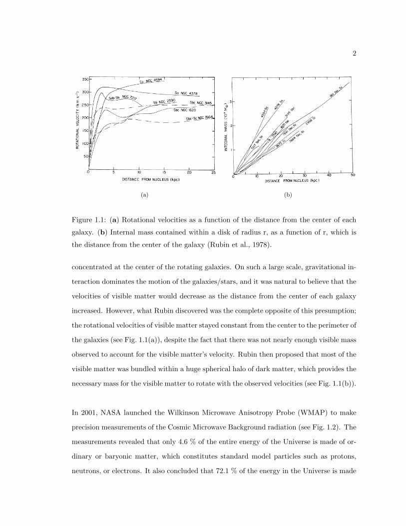
Figure 1.1: (a) Rotational velocities as a function of the distance from the center of each
galaxy. (b) Internal mass contained within a disk of radius r, as a function of r, which is
the distance from the center of the galaxy (Rubin et al., 1978).
concentrated at the center of the rotating galaxies. On such a large scale, gravitational in-
teraction dominates the motion of the galaxies/stars, and it was natural to believe that the
velocities of visible matter would decrease as the distance from the center of each galaxy
increased. However, what Rubin discovered was the complete opposite of this presumption;
the rotational velocities of visible matter stayed constant from the center to the perimeter of
the galaxies (see Fig. 1.1(a)), despite the fact that there was not nearly enough visible mass
observed to account for the visible matter’s velocity. Rubin then proposed that most of the
visible matter was bundled within a huge spherical halo of dark matter, which provides the
necessary mass for the visible matter to rotate with the observed velocities (see Fig. 1.1(b)).
In 2001, NASA launched the Wilkinson Microwave Anisotropy Probe (WMAP) to make
precision measurements of the Cosmic Microwave Background radiation (see Fig. 1.2). The
measurements revealed that only 4.6 % of the entire energy of the Universe is made of or-
dinary or baryonic matter, which constitutes standard model particles such as protons,
neutrons, or electrons. It also concluded that 72.1 % of the energy in the Universe is made

3
Figure 1.2: Seven year WMAP data showing the temperature fluctuations that occurred
13.7 billion years ago (The WMAP Science Team).
up of Dark Energy, which is believed to be responsible for the acceleration of the Universe’s
expansion. The remaining 23.3 % of energy is believed to be made up of Dark Matter, the
subject of this thesis (Komatsu et al., 2010; Bennett et al., 2003).
More evidence for the existence of Dark Matter came from weak gravitational lensing ob-
servations of two colliding clusters of galaxies, called the ’bullet cluster.’ In their paper,
Clowe et al. presented the analysis of the details of the two colliding galaxies (Clowe et al.,
2006). The two galaxies collided with a velocity of 4500 km/s. After the collision, there is a
clear separation between the concentrations of visible matter and the invisible matter. The
green lines in Fig. 1.3 show the gravitational contour based on weak lensing measurements
and the distribution of Dark Matter is depicted in blue. During the merging event of the
two clusters, ordinary gas experienced ram pressure, and the motion of the visible part of
the galaxies slowed. This is shown in the color plots of Fig. 1.3. However, Dark Matter
does not experience such a force, resulting in the clear separation of the two species of
particles baryonic and non-baryonic matter. This phenomenon presented strong evidence
for the existence of Dark Matter. There is no question that the majority of the matter
in the Universe consists of non-baryonic cold Dark Matter (Bertone et al., 2005). Dark

4
(a) (b)
Figure 1.3: (a) The merging cluster 1E0657-558. (b) Image from NASA’s Chandra X-ray
Observatory (Clowe et al., 2006).
Matter is some type of matter that is heavy enough to cause the orbital velocity of galaxies
to be constant, regardless of the distance from galaxies’ centers and the amount of visible
matter within the galaxies.
If Dark Matter does exist, it is very likely that it would follow new physics laws beyond
the Standard Model of particle physics. One of the leading candidates of Dark Matter is
called Weakly Interacting Massive Particles (WIMPs) (Jungman et al., 1996). WIMPs are
stable, carry zero electric charge, and interact weakly with baryonic matter. One of the
theories that attempts to explain Dark Matter beyond the Standard Model of physics is
the theory of Supersymmetry. According to this theory, the lightest supersymmetric par-
ticle (LSP) is the Dark Matter particle and would interact with ordinary matter through
extremely small interaction cross sections. In this model, the conserved quantum number
(called R-parity) prevents such LSP particles from decaying into ordinary baryonic matter.
They are therefore considered to be stable over the life of the Universe.

5
1.2 General Detection Method
1.2.1 Detection Technique
There are three ways to look for Dark Matter. One is with a particle collider such as
the LHC (Kane and Watson, 2008), which is expected to make new discoveries in particle
physics. Another detection method is ’indirect detection.’ Such experimental methods
include the Alpha Magnetic Spectrometer (AMS) project (Alcaraz et al., 1999). In an
indirect detection method, the detectors are launched into outer space and look for WIMP
annihilation products. The big challenge in such an experiment is the separation of the
Dark Matter signal from the large background that originates in astronomical events such
as supernovae. Finally, the method we utilize is called ’direct detection’ of Dark Matter
(Gaitskell, 2004). This detection method relies on Dark Matter’s interaction with target
nuclei through its extremely weak interaction rate. We attempt to detect the scattering of
the target nucleus and energy deposited as it recoils from a collision event with an incoming
Dark Matter particle.
The expected mass of Dark Matter candidates varies from a few GeV to hundreds of
GeV(Bertone et al., 2005). In our experiment, we use a time projection chamber (TPC)
filled with low pressure carbon tetrafluoride (CF4) gas. Typical WIMP-induced nuclear
recoils in such a detector are expected to deposit energy of a few to 100 keV. Dark Matter
interactions with ordinary matter would occur through either axial (spin-dependent) or
scalar (spin-independent) interactions (see Fig. 1.4). Through the spin-dependent interac-
tion with Dark Matter, a fluorine atom is considered to be the most sensitive candidate
(Ahlen, 2010). The next most sensitive target would be Xe, followed by iodine and ger-
manium. It has been shown that an LSP Dark Matter candidate may have a fairly large
cross section through the spin-dependent interaction (Moulin et al., 2005; Gainer, 2010).
As I will discuss later in Sec. 2.2, CF4 gas is known for its good scintillation efficiency, low
transverse electron diffusion effect and is non-flammable and non-toxic; thus, using fluorine

6
(a) (b)
Figure 1.4: Expected cross sections calculated in non-MSSM model of (a) spin-dependent
and (b) spin-independent interactions on nucleon (Moulin et al., 2005).
as the target gas for the direct detection is a great advantage.
1.2.2 Daily/Seasonal Modulation
In our direct detection method, we attempt not only to identify the energy deposited by
Dark Matter induced nuclear recoils, but also the direction of those recoil particles. In a
simple Dark Matter halo model, our Solar System rotates around the center of the Milky
Way Galaxy with a velocity of approximately 220 km/s within a spherical halo of Dark
Matter. In this orbital motion, the direction of the Solar System is pointing towards the
constellation Cygnus. Under the simple non-dissipative Dark Matter halo model, the Dark
Matter particles are expected to be distributed by the Maxwell-Boltzmann distribution
(Navarro et al., 1996; Ullio and Kamionkowski, 2001). From our reference frame on Earth,
it seems as if our Solar System is moving through a sea of Dark Matter, due to the rota-
tional motion of the Solar System around the center of the Milky Way Galaxy. Thus, the

7
Figure 1.5: Illustration of an annual modulation. The Earth rotates around the Sun with
the rotational inclination of roughly 60 degrees relative to the motion of the Solar System
itself rotating around the center of the Milky Way Galaxy.
direction of the Dark Matter flying towards us seems to originate from the direction of the
constellation Cygnus. This is called Dark Matter wind. Because the Earth spins on its
axis of rotation, the direction of Dark Matter wind changes continuously. This is called a
daily modulation. In our experiment, we put emphasis on the directionality characteristics
of Dark Matter wind due to the daily modulation effect.
The Earth rotates around the Sun with an inclination of roughly 60 degrees relative to
the plane of rotational motion of the Solar System around the center of the Milky Way
Galaxy. When the vector of the Earth’s motion lines up with that of the Solar System,
the net Earth rotational velocity with respect to the rest of the Milky Way Galaxy reaches
its maximum. This occurs during summer time in the northern hemisphere (see Fig. 1.5).
Conversely, the total velocity reaches its minimum during the winter, so the amplitude of
the Earth’s total velocity relative to the galactic rest frame fluctuates up to a few percent
throughout the entire year. This is called an annual modulation. If Cold Dark Matter

8
Figure 1.6: The annual modulation measurement of Dark Matter signals from
DAMA/LIBRA (Bernabei et al., 2008).
is indeed distributed in the way mentioned above, the velocity of the Dark Matter par-
ticles flying towards us from the direction of the constellation Cygnus would fluctuate
accordingly. Thus, the energy spectrum of Dark Matter induced nuclear recoils for the
elastic scattering events would also fluctuate due to the annual modulation (Drukier et al.,
1986; Freese et al., 1988). DAMA/LIBRA claims that they measured this Dark Matter
induced annual modulation signal in their experiment (Bernabei et al., 2008). Their mea-
surement shows the annual modulation of the signal amplitude (see Fig. 1.6). However,
their claim has not been broadly accepted. Because background particles such as neutrons
would strongly mimic the elastic scatter of Dark Matter particles of target nuclei, their
measurements are too ambiguous to argue convincingly that they have only recorded the
Dark Matter signals. DAMA’s result has also been excluded by other experiments such as
XENON100 or CDMS (Aprile et al., 2010).
In order to make a clean identification of Dark Matter particle collision events, one needs
to employ a technique that neatly separates the actual Dark Matter signals from back-
ground noise. The technique we use is called a daily modulation (see Fig. 1.7). Due to
the daily motion of the Earth, a detector on the Earth’s surface would observe the direc-
tion of the incident Dark Matter wind to shift accordingly. For example, for a detector

9
Figure 1.7: Illustration of a daily modulation. Due to the change of the detector position
over 12 hours, the direction of the Dark Matter wind shifts accordingly (Sciolla, 2009).
placed in Boston, the Dark Matter wind direction changes by roughly 96 degrees over
12 hours. Thus, if one had the capability of detecting the direction of the Dark Matter
wind, the direction of the resultant signal would shift by the same amount. Showing this
result together with the energy spectrum due to the Dark Matter velocity would provide
unambiguous evidence for the existence of Dark Matter. Although it is very important to
identify background particles such as neutrons, only Dark Matter particles would produce
such a shift of the incident direction presented by the daily modulation. The anticipated
Dark Matter signal with directionality by the daily modulation is much more obvious than
the data relying only on the seasonal modulation. Mere event rate comparison of forward
and backward direction oriented Dark Matter signals gives roughly an order of magnitude
difference (Spergel, 1988).
1.2.3 Other Capabilities of the Detector
So far I have only mentioned the direct detection of an elastic collision of Dark Matter off
the target nuclei. Recently, however, the possibility of Dark Matter inelastic collisions have
also been pointed out (Cui et al., 2009; Chang et al., 2009). The basic assumption in this
theory is that the Dark Matter particles would have both ground and excited states that

10
are separated by roughly 100 keV. When the coherent inelastic scatter occurs, the Dark
Matter particle gets shifted into its higher energy state. Because of the inelastic collision, a
new particle, heavier than Dark Matter, will be formed and continue moving in the incident
direction of the Dark Matter particle. In their model of Dark Matter, with a Dark Matter
particle mass of 250 GeV, Chang et al. estimated an expected count rate of 0.5 /kg/day.
Essentially any experiment with a direct detection method could be integrated into this
technique. In our experiment, the use of Xe gas would be ideal for this method because the
expected Dark Matter mass is rather close to that of the target Xe atoms. Furthermore,
no changes would have to be made to our detector in order to search for inelastic collisions;
we would simply switch the target gas from CF4 to Xe. Because Xe is very heavy, it would
not be too difficult to reach a high target mass with our TPC detector. Although very
preliminary, I will show the first study of our prototype Dark Matter detector with Xe gas
later in this dissertation (see Chap. 5).
As mentioned earlier, among all the backgrounds in Dark Matter detection, neutron-
induced nuclear recoils are the worst because they mimic those from Dark Matter. In
Dark Matter experiments, it is very important to shield the detector actively and/or pas-
sively from the neutron background. One effective method to achieve this goal is to place
the detector deep in a mine so that one can minimize the effect of the cosmic ray back-
ground. In this dissertation, I will discuss and quantify our detector’s background neutron
measurements capability, which is necessary for the DMTPC Dark Matter experiment.

Chapter 2
DMTPC Detection Method
2.1 Fundamental Detector Concept
The DMTPC (Dark Matter Time Projection Chamber) collaboration involves physicists
from Boston University, Brandeis University and Massachusetts Institute of Technology.
The basic idea of the DMTPC detector concept is shown in Fig. 2.1. The main components
of the detector are the anode plate, grid mesh, cathode mesh and field cage rings. Positive
high voltage is applied onto the anode, whereas the grid mesh is held at ground (potential);
thus, a very intense electric field is created between the two. Inside the detector is filled
with low pressure CF4 gas.
When a Dark Matter particle collides with a fluorine nucleus in the detector, it transfers
some energy and momentum to the fluorine recoil with typical energies on the order of a
few tens of keV. In the inelastic Dark Matter model, the target gas would be Xe. For a neu-
tron detector, it works exactly the same except that most of the elastic scattering events
occur off target helium atoms of an added 4He gas because of 4He’s large cross section
with neutrons. In a low pressure TPC at 40 torr CF4 gas, a Dark Matter-induced fluorine
recoil results in a length on the order of a couple of millimeters. When an incident Dark
Matter particle collides with a fluorine nucleus, the nucleus is liberated and recoils with
some kinetic energy, accompanied by one or more electrons. When this positive ion travels
11

12
Figure 2.1: Schematic of the DMTPC Dark Matter detection method.

13
through the gas, it loses energy by ionizing other atoms and molecules along its path. CF4
has a W value of 54 eV, so the traveling ion loses kinetic energy by an average of 54 eV at
each ionization event along the path. The cathode mesh is kept at negative high voltage so
that the ionization electrons will travel towards the grounded grid mesh and into the ampli-
fication region. When they reach the amplification region, which has a much more intense
electric field than the drift region, those ionization electrons multiply (electron cascade)
with a typical gain of 104 to 105. These so-called ’avalanche’ electrons excite ions of CF4
and cause scintillation of red light to occur (Pansky et al., 1995; Fraga et al., 2003). The
photons emitted from this event travel towards the charge-coupled device camera (CCD
camera) and photo multiplier tube (PMT) and will be captured as a light signal by those
devices. The lens attached to the CCD camera is set to focus on the amplification region
so that the 2D particle track projection onto the amplification region will be captured as
data by the CCD camera. Although it depends on what type of particle is being measured,
a typical charged particle in our experiment with an energy less than the order of MeV
will travel only on the order of nanoseconds or less before it comes to rest. This is short
compared to the drift time of the electrons as they move toward the anode. When the
first light signal above the threshold from either head or tail of the moving particle hits the
PMT, it triggers both the CCD and PMT to start recording the information. The camera’s
minimum exposure time achievable is at least a factor of 100 greater than the actual time
of particle motion; thus, there is no ambiguity about whether the particle is fully or only
partially contained within the CCD image as long as the track occurred within the cam-
era’s view. Because the PMT is a fast device, it has no problem obtaining an unambiguous
signal from the drifting electrons in the detector. Depending on the vertical component of
the travelling particle, PMT signals can come in various shapes over time, but they will
measure the time between the arrival of the first and last electron at the amplification stage.
14
(a) (b)
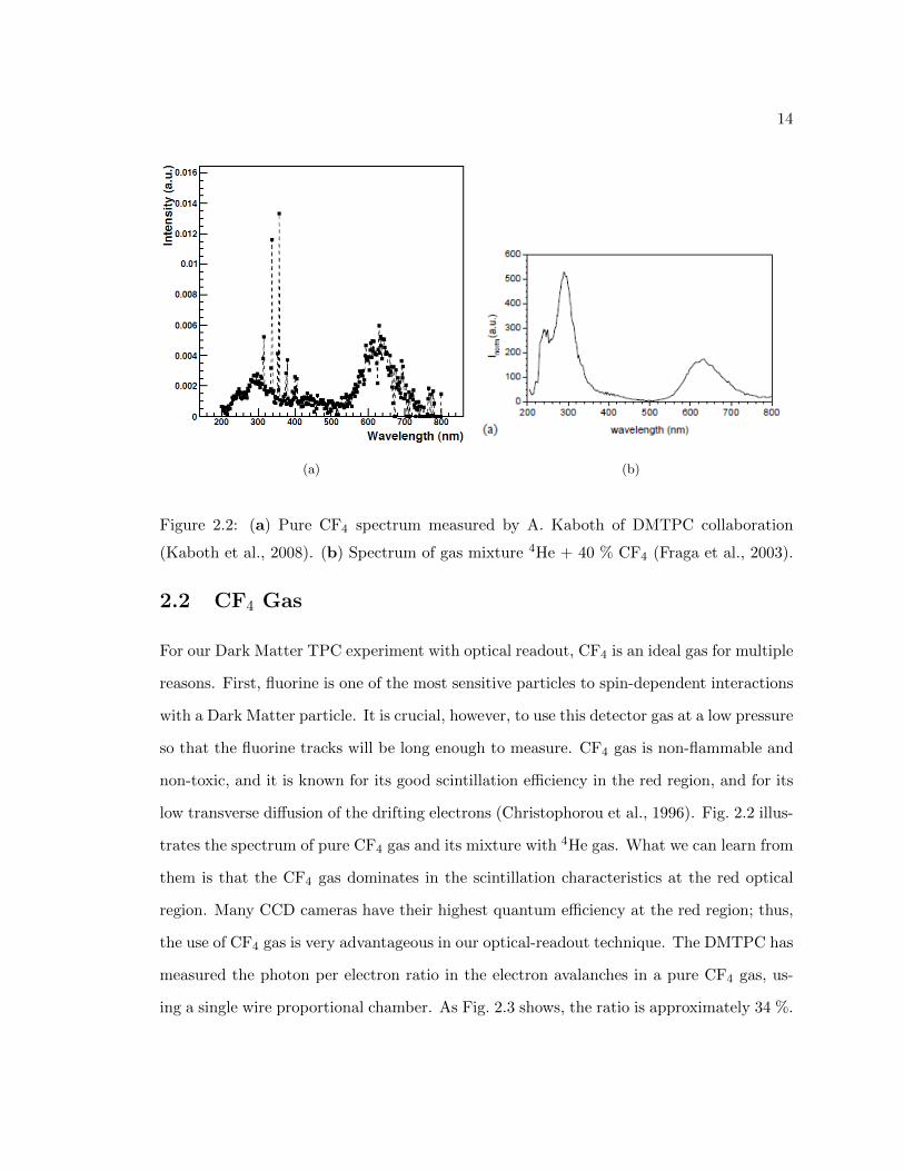
Figure 2.2: (a) Pure CF4 spectrum measured by A. Kaboth of DMTPC collaboration
(Kaboth et al., 2008). (b) Spectrum of gas mixture 4He + 40 % CF4 (Fraga et al., 2003).
2.2 CF4 Gas
For our Dark Matter TPC experiment with optical readout, CF4 is an ideal gas for multiple
reasons. First, fluorine is one of the most sensitive particles to spin-dependent interactions
with a Dark Matter particle. It is crucial, however, to use this detector gas at a low pressure
so that the fluorine tracks will be long enough to measure. CF4 gas is non-flammable and
non-toxic, and it is known for its good scintillation efficiency in the red region, and for its
low transverse diffusion of the drifting electrons (Christophorou et al., 1996). Fig. 2.2 illus-
trates the spectrum of pure CF4 gas and its mixture with 4He gas. What we can learn from
them is that the CF4 gas dominates in the scintillation characteristics at the red optical
region. Many CCD cameras have their highest quantum efficiency at the red region; thus,
the use of CF4 gas is very advantageous in our optical-readout technique. The DMTPC has
measured the photon per electron ratio in the electron avalanches in a pure CF4 gas, us-
ing a single wire proportional chamber. As Fig. 2.3 shows, the ratio is approximately 34 %.

15
Figure 2.3: A linear fit to the number of photons vs. number of electrons from the electron
avalanche in the detector’s electron amplification region (Kaboth et al., 2008).
The number of photons acquired from a single fluorine recoil may be approximated in the
following equation. For this estimation, I assume all the parameters as explained below.
γ = Krecoil × 12 ×
1WCF4
×Ge×Effe→γ × Slens4 π D2×Tlens×Twindow×QE×Tgrid×Tcathode
Krecoil (recoil fluorine energy) = 30 keV
WCF4 (average energy to produce electron-ion pair in CF4 gas = 54 keV
Ge (gas electron gain) = 105
Effe→γ (scintillation efficiency) = 0.34
Slens (lens surface area - assume use of Canon 85 mm f/1.2 lens) = 47
D (lens-to-anode distance in cm) = 35
Tlens (lens transmittance in the red region) = 0.85
Twindow (glass window transmittance in the red region) = 0.9
QE (quantum efficiency of the Apogee U6 camera) = 0.65
Tgrid (grid mesh spatial transmission) = 0.8
Tcathode (cathode mesh spatial transmission) = 0.8

16
In this simple model, it is suggested that we would acquire 9,200 photons from a 30 keV
fluorine recoil induced by the collision with a Dark Matter particle. The combination of
the Canon 85 mm lens and Apogee Alta U6 camera is being used as a part of our DMTPC
detector in the WIPP (Waste Isolation Pilot Plant) mine in Carlsbad, New Mexico for
the initial background study. In a typical setup, each CCD pixel maps about 300 µm by
300 µm of real space, and a 30 keV recoil would be distributed over about 10 pixels, so
each pixel will contain an average of 920 photoelectrons. The Alta U6 camera has a typical
RMS readout noise of 8 electrons; thus, the typical signal-to-noise ratio of such a detector
would be as large as 115.
In our standard data taking, we employ a pressure of 40 torr for the CF4 gas in the detec-
tor. This is a low enough pressure that typical Dark Matter-induced fluorine recoils with
energies of the order of tens of keV will travel for a couple of millimeters. This enables us
to observe the recoil track with directionality. An even lower pressure would work better
in terms of the ratio of particle track length vs. track width after some transverse elec-
tron diffusion; however, when the pressure of CF4 gas becomes too low, we begin to face
discharge problems in our high voltage amplification system before reaching enough gain
in this region. Unfortunately, not much is known about the electric discharge mechanism,
especially with the specific gas mixture and pressure settings we are interested in using
with CF4 gas. After some trial-and-error, we have come to the conclusion that 40 torr of
CF4 gas pressure is the optimum combination and has become our standard data-taking
mode for the TPC chamber. It is also hard to get large detector mass with very low pressure.
Our detector relies on the scintillation light that occurs from the drift and cascade electrons
exciting the CF4 gas molecule ions. When a charged recoil particle travels through such a
gas detector, it continuously loses its energy along its path by ionizing the gas atoms and
molecules. However, it does so at different rates along its trajectory (see Fig. 2.4). When
17
the energy of the recoil particle is greater than the so-called ’Bragg peak’ energy, its rate of
energy loss increases as it loses energy. When it reaches the Bragg peak energy, where the
particle is losing the greatest amount of energy per unit distance travelled, the ionization,
as well as subsequent light collected, is at its greatest value. If the particle starts with
energy less than the Bragg peak energy, the energy loss per unit distance travelled, and
light collected along the path, will decrease along the path. With the knowledge of this
light distribution along the path length for either situation, we can identify the direction
of moving particles, which we call a ”head-tail” effect (Dujmic et al., 2008).
After the ionization event in the TPC, the ionization electrons start traveling against the
direction of the drift electric field created in the field cage. During this drifting motion,
each electron makes copious numbers of collisions with the electrons of the gas molecules.
This causes the trajectory of each electron to be not straight; thus, the electrons are mov-
ing towards the amplification region taking random paths. In effect, when the stream of
electrons from the initial particle ionization track reach the amplification region for the
scintillation, the measured transverse width of the particle track becomes much wider than
what it really is. This is called electron diffusion, and it is related in a non-linear fashion
with how far the electrons have drifted, what the pressure of the gas is, and the strength
of the drift electric field (Christophorou et al., 1996; Ahlen, 2010). The amount of electron
diffusion can be described in the following equation.
σdiffusion =√
ZN ·
√2 Dµe
NE
Z: electron drift distance
N: number density of molecules
D: transverse electron diffusion constant
µe: electron mobility
E: drift electric field

18
Figure 2.4: An α particle travelling from left to right through the gas mixture of 40 torr
CF4 and 600 torr 4He. The black histogram represents the actual data from the above
CCD image, which shows the great agreement with the SRIM Monte Carlo simulation
(The Stopping and Range of Ions in Matter) of the stopping power (red markers). Three
locations where the particle track is being cut are due to the 530 µm fishing wires as spacers
between the anode and grid. The energy of the α particle is about 4.8 MeV, and at such a
low energy, the stopping power can be approximated by the Bethe-Bloch formula presented
in the above plot.

19
Figure 2.5: The rate of electron diffusion coefficient over the electron mobility as a function
of the drift electric field applied over the number density of CF4 gas (Christophorou et al.,
1996).
Fig. 2.5 shows the relationship between the amount of electron diffusion coefficient and
the drift electric field applied in CF4 gas. Our MIT collaborators have carried out an
experiment measuring the electron diffusion relative to the applied drift electric field in the
pure CF4 gas detector. In this setup, five 241Am α sources were placed in the electron drift
region in such a way that each of the electron drift length would be 2 cm, 5 cm, 10 cm,
13 cm, and 17 cm in pure 75 torr of CF4 gas in the detector (see Fig. 2.6). The red markers
in Fig. 2.7(b) are from our own data (see Fig. 2.7(a)), and one can see how closely our data
matches the expected value. Backed up by this result, the best setting of drift electric field
that minimizes the electron diffusion in 40 torr of CF4 gas is 125 V/cm. Because there
is a limit to how low one can decrease the particle tracks’ diffusion values, it is crucial to
keep the recoil track length long enough for us to be able to tell the direction of the path.
Similarly, this also means there is a maximum limit of the drift length that we can use
in our detector. The problem of the electron diffusion is not confined to establishing the
particle tracks’ direction of motion. When diffusion occurs, the light level of the edge of
the particle tracks captured in the CCD image goes below the typical thermal and readout
noise level of the CCD. If the drift distance is large, the energy and length of the particle

20
Figure 2.6: The transverse electron diffusion is measured along the two black lines in the
figure, which represent a 1.2 mm wide region of interest (Caldwell et al., 2009).
track observed and analyzed become smaller than what they really are, and it will lower
the energy and spatial resolution of the detector.
2.3 Neutron Detection
As I already mentioned at the beginning of this dissertation, neutrons are the greatest
background for this type of direct detection Dark Matter detector. In order to understand
our detector well, we must fully comprehend how neutrons interact in our detector. Dur-
ing our research, we have come to realize that our Dark Matter detection method can also
be utilized to detect neutrons with great efficiency and a good sense of directionality. Al-
though pure CF4 gas is the best choice for our Dark Matter experiment, this is not the case
for a neutron detector. Neutrons have a greater cross section with helium. For this type
of detector, helium gas, being inert and stable, is among the best target gases for mixing

21
(a) (b)
Figure 2.7: (a) A linear fit to σdiffusion2 as a function of the drift distance. (b) DMTPC
data comparison to others (Caldwell et al., 2009).
with CF4 gas. Thus, 4He gas is the most suitable for fast neutron detection because of its
large cross section (see Fig. 2.8) and low mass, which enables it to absorb large energy in
neutron collisions. 3He would be the most suitable in detecting thermal neutrons due to
its enormous cross section in the thermal neutron absorption events (see Fig. 2.9), but it
is quite expensive. In the mixture of either 3He or 4He gas, we still use 40 torr of CF4 gas
as our standard setup because helium gas by itself does not scintillate strongly enough in
the spectrum region to enable us to take a good measurement, but helium gas serves as a
neutron capturing medium because of its large cross section with neutrons.

22
Figure 2.8: Elastic neutron scattering cross sections of carbon, fluorine, and 4He (National
Nuclear Data Center, Brookhaven National Laboratory).
Figure 2.9: Elastic neutron scattering cross sections of carbon, fluorine, and 3He, in com-
parison to the much larger 3He absorption cross section (black solid line) (National Nuclear
Data Center, Brookhaven National Laboratory).

Chapter 3
DMTPC Detector
3.1 Detector Introduction
Historically in experimental particle physics, optical measurements of particle tracks have
been employed. Bubble chambers and cloud gas chambers are examples. Now, thanks to
the development of technology, CCD camera images are suitable for detecting and analyz-
ing nuclear recoils and their directionality. This is because the grid of pixels that makes
up the CCD collects light in a linear fashion, and has an extremely high spatial resolution
on the order of hundreds of micrometers per pixel. Another essential advantage of using a
CCD camera as the image readout device is its superior quantum efficiency.
Typical CCD chips have quantum efficiencies higher than 60 % in the optical region. Our
most up-to-date detector prototype, which I will discuss in more detail later, has a quan-
tum efficiency of greater than 90 % with red light. When the camera is triggered either
internally or externally, the optical image transmitted by photons is saved into each CCD
grid as an electrical charge in the CCD’s electrical potential well. Once it reaches the set
exposure time, a CCD starts reading out those electrical charges row by row and column
by column, resulting in the mapping image of light intensity. There are, roughly speaking,
two types of shuttering mechanisms in CCD cameras; one is called nonframe-transfer, and
the other frame-transfer CCDs. Nonframe-transfer CCDs are usually equipped with me-
23

24
chanical shutters. Those shutters open when the camera receives an open exposure signal,
and mechanically close after the set exposure time is spent. The advantage of such cameras
is that once the shutter is closed, there is no more light entering the light sensing area of
the CCD chip. However, due to the shutter speed, one usually cannot set a very small
exposure time. Frame-transfer CCDs, on the other hand, can be set to an extremely small
exposure time. Unfortunately, because there is no mechanical shutter to prevent light from
entering the light sensitive area during the data readout period, this leads to a possible
misidentification of particle location by one pixel row or more if there are more than two
particle tracks recorded in a single image file. This is because one track triggers the camera
and others may happen during the data readout time.
Although the use of a CCD camera is very suitable for particle detection based on its
optical detection technique, the 2D nature of the image retrieved from a CCD makes it
difficult to distinguish the vertical component of the travelling particle moving through the
gas chamber from this information alone. In other words, when a particle with a given
energy moves more vertically through the chamber, with a CCD image alone, it is difficult
or impossible to distinguish it from a particle with more energy that is moving in a less
vertical direction (see Fig. 3.1). In order to compensate for this disadvantage, we read the
PMT signal for each event in addition to the optical CCD track image. Signals captured
by a PMT are very useful in determining the timing of the interaction and duration of the
drifting electrons. The typical time scale of these events is on the order of microseconds or
less. Using this PMT information along with the corresponding CCD particle track image
successfully, we can recreate the three-dimensional information of each recoil track.
Another important use of the PMT is to exploit it as a trigger for the entire system. Be-
cause PMT signals can be read and analyzed in a trigger mode with high speed (∼10 ns)
compared to the CCD readout (∼10 ms), it is convenient to use the PMT to trigger the
CCD camera, as well as a waveform digitizer, to record the pulse shape obtained by the

25
(a) (b)
Figure 3.1: Comparison of particle tracks (a) horizontally moving and (b) vertically mov-
ing. Particles from both images show a combination of proton and triton tracks due to a
thermal neutron capture event of 3He.
same or other PMTs as described in Fig. 3.2. This setup has the added benefit of allowing
the camera to continually flush and clean its pixel information until the trigger pulse is
received, thereby minimizing the thermal noise in each CCD image. This combination
system has been selected among other experimental setups of the camera and PMTs due
to the maximization of a frame rate, the speed of events recording, and the quality of data.
In addition to particle interactions due to elastic collisions, another important application
of our device, especially as a neutron detector, is the measurement of inelastic collisions.
When a high energy cosmic ray or fissile neutron collides with the nucleus of a detector
gas atom and transfers enough energy into the nucleus, it can cause the atom to split into
two or more lighter ions. We can capture this kind of event in a very robust way with
the help of the PMT pulse information, as well as the CCD’s optical images. This lets us
measure the inelastic collision cross section and the flux of high energy cosmic ray neutrons.

26
Figure 3.2: Schematics of a typical triggering/data-taking system.
3.2 First R&D Wire Chamber at MIT
I joined the DMTPC collaboration in the summer of 2006, by which time, a large part of
the conceptual work and the basics of this detection method had already been developed.
However, our first R&D Dark Matter experiment test chamber was extremely primitive
compared to what we have now. It was equipped with only a small CCD camera with a
view of 1 cm by 1.5 cm and, in order to achieve good spatial resolution and light collection,
a typical drift length on the order of centimeters. Instead of the current mesh system, we
were experimenting on a metallic ’wire’ system.
Our first R&D vacuum chamber was a custom made LACO tech chamber with the capa-
bility of reaching millitorr range in vacuum after one day of pumping out with a turbo
molecular pump (see Fig. 3.3). Inside the chamber was our very first hand-stretched wire
amplification region. Two types of wire planes were made, with a 25 µm and 100 µm
diameter respectively. The wires were installed with 5 mm spacing onto the 10 cm by
10 cm opening of a G-10 board. Initially, the gap distance in the amplification region,
applied voltage, and the gas pressure of the chamber were varied for the tests based on
the electric field simulation so that we could get enough gain. But it was important not to

27
Figure 3.3: Our first R&D Time Projection Chamber from LACO technology in MIT. The
10 cm by 10 cm wire planes (anode and grid) can be seen through the cathode mesh in the
middle. A CCD camera was attached to the top of the chamber, looking down into the
chamber through a glass window. Regular G-10 boards were used to attach the mesh and
wires.

28
Figure 3.4: Quantum efficiency curve for the Kodak KAF-0401 CCD chip (Eastman Kodak
Company).
apply too high an electric field; otherwise, we would end up with frequent sparking events.
Our first CCD camera for this R&D was a simple and inexpensive one from Finger Lake
Instrumentation, which cost about $2,000. It was equipped with Kodak KAF-0401 CCD
chip with 768 by 512 numbers of pixels. The size of each pixel was 9 µm by 9 µm, and the
CCD camera was capable of cooling down the chip to negative 20C in room temperature.
Although the CCD chips were made specifically for the red region, the actual quantum
efficiency was only 35 % (see Fig. 3.4).
A regular 55 mm Sears photographic lens was attached to the CCD camera. An 241Am
α source was extracted from a generic smoke detector and placed so that the α particles
traveled directly across the drift region. Although the basic theory of the scintillation
mechanism had already been established, we had not been successful capturing the actual
ion track from an 241Am α particle source. After a series of trials, we succeeded in captur-
ing our first α particle track in an optical image, proving that our technique works. During
this time, we learned that the cleanliness inside the chamber was essential for maintaining
gas quality, and we minimized the possible leakage in the vacuum chamber and discovered
the significance of pumping out the chamber for a long period of time. When a vacuum

29
Figure 3.5: Schematics of our first TPC system. The electron drift region was only on
the order of a couple centimeters with no field-shaping device. In order to avoid sparks,
we started with fairly large amplification gap on the order of several millimeters at the
sacrifice of the electron gain.
chamber is pumped down to low pressure, the impurities, mainly water, start coming out
of the surface of the chamber and cause the detector gas inside to degrade. This is called
outgassing. One can never achieve zero outgassing level; however, by pumping out for a
long time or using the right material, the gas impurity level in the vacuum chamber was
sufficiently low to allow data taking. Fig. 3.5 is the schematic of our very first R&D TPC
system. The ground plate at bottom in the figure is no longer in use in our TPC system.
The dimensional specifications of the successful TPC prototype were as follows: anode
frame was made with 100 µm diameter wires at 5 mm of spacing, grid (ground) wires were
made with 25 µm diameter wires at 2 mm of spacing to each other, and the cathode was
made with mesh of 25 µm stainless steel wires at 250 µm pitch because there was very little
difficulty in using mesh for the cathode; imperfection in stretching the mesh does not affect
the integrity of the system. For this test, we used -1 kV for the cathode and +2.25 kV for
the anode. The locations of the devices are shown in Fig. 3.5. The chamber was filled with

30
Figure 3.6: One of our very first optical images of an ion (α particle) travelling through
low-pressure CF4 gas, and the scintillation due to the electron cascade captured by our
CCD device. The α particle starts from the top-right of the view to the bottom-left. Only
a partial track is captured within the image because of the small field of view.
CF4 gas at 37 torr, which is in the range of gas pressure we are interested in the search for
Dark Matter. Due to the limited quality of the CCD camera and gain available from our
very first TPC amplification system, we had to place the lens as close to the amplification
region as possible on the other side of the viewing port, so the actual viewing size was very
small. Fig. 3.6 is the first image of an α particle track captured in our R&D prototype
chamber, where the α particle was moving from right top to left bottom in the view. The
CF4 gas purity level was essential for this successful optical measurement of the α particle
tracks.
In Fig. 3.6, the actual size in scale is 2.5 cm horizontally and 1.7 cm vertically, and an
electron multiplication gain reached on the order of 104. However, in order to have an ac-
ceptable signal-to-noise ratio and capture clear images, software binning was necessary. A
software binning is a method of combining neighboring multiple pixel information together
in order to reach a higher gain at the sacrifice of spatial resolution. In this image, the
actual image superpixel size was approximately 200 µm by 200 µm. In order to include

31
as many scintillation spots as possible, I rotated the CCD camera to an angle relative to
the direction of the anode wires. In Fig. 3.6, the 241Am α source was placed in such a way
that the α particle traveled transverse to the direction of the anode wires. As mentioned
earlier, the spacing of the anode wires was kept at 5 mm, so the distance between each
scintillation spot in Fig. 3.6 was 5 mm.
When an α particle moved through gas inside the experimental chamber, it ionized the
atoms along its path. If the particle traveled parallel to the direction of the wires, the
ionization electrons scintillated along the wire, which was the path of the moving particle.
On the other hand, if the particle moved perpendicular to the direction of the wires, it
would leave pin points of the scintillation as shown in Fig. 3.6. Although the wire chamber
worked beautifully, the spatial resolution of particle tracks was relatively poor. Also, the
variation in wire spacing caused variations in gain; thus, it was very difficult to achieve
good energy resolution. Furthermore, we did not have much knowledge about the purity
of gas in the chamber at that point. However, we successfully captured signals from α par-
ticles optically. This proved that the fundamentals of our detection concept and method
would work rather beautifully due to the robustness and simplicity of the detector, and
the optical particle image readout by a CCD camera.
After the first success of capturing the α particle track images with this wire chamber, we
made an attempt to make a mesh anode plane. The basics of the design were the same,
but with the mesh plane we could achieve much higher spatial resolution. This attempt
turned out to be very challenging because we had no organized method of stretching out
a mesh plane with equal tension in all directions. In order for the mesh plane to work,
the gap distance in the amplification region had to be extremely small; otherwise, the cas-
cade electrons would be spread out in much greater area compared to the wire chamber’s
case, resulting in the lower electron gain per unit area. In order to overcome this problem
and decrease the amplification distance gap, it was necessary to stretch out the mesh very

32
uniformly with greater tension. And at this point, we did not have a good method or
knowledge of doing so. Thus, in parallel to continuing working on a mesh plane develop-
ment, we pursued the wire plane readout method.
3.3 Prototype Dark Matter Detector at Boston University
3.3.1 First Wire Chamber Components
After our first success in proving the basics of our TPC detection mechanism, we began
building our first prototype detector at Boston University (see Fig. 3.7). Our first task was
to build what we had at MIT, but with improvement in quality and design. One example
of the material selection was seeking out material with a low outgassing quality. In order to
minimize outgassing of water vapor, the inner surface of the vacuum chamber from Kurt
J. Lesker, Co. was electropolished. The TPC components were made out of aluminum
or stainless steel plates as much as possible, and the wires were glued directly onto the
aluminum frames with an inner opening of 20 cm by 20 cm with a thickness of 1.6 mm (see
Fig. 3.8). We glued the wires onto the frame with 3M’s DP460EG low outgassing epoxy.
This epoxy cures at room temperature over 24 hours and has sufficient strength to hold
the wires in place. The wires were professionally stretched at Brookhaven National Lab
(BNL) and glued onto an aluminum transfer frame of 48” by 52” (see Fig. 3.9). The frame
and wires were returned to Boston University so that we could transfer the wires directly
onto our own aluminum TPC frames (see Fig. 3.8). We had learned from our very first
MIT R&D chamber about the importance of uniformity in spacing and tensioning of the
wires, a uniformity which cannot be achieved by hand. With the wire winding machine at
BNL, we had the wires stretched to a uniform tension of 100 g with a uniform spacing of
2.5 mm. For this operation, we used two different wires with different diameters; 50 µm
gold-plated rhenium wire and 30 µm gold-plated tungsten wire. With 100 g of tension, the
natural sagging of the wires within the aluminum TPC frame due to gravity is minimal,

33
less than 2 µm for the Re-Au wire, and less than 1 µm for the W-Au wire. The breaking
stress of the above wires is 600 g for the Re-Au wire and 200 g for the W-Au wire. In
the amplification region, the electric field increases dramatically near the surface of the
wire with a rate of inverse radius squared. We estimated that the electric field of greater
than 106 v/m was required to have enough gain to view particle tracks. However, if the
electric field becomes too great, the intense electric field is prone to the discharge problem.
Any surface defect of the wires could cause the charges on the anode wires to find a path
through gas onto the ground wires as a spark event. Thus, we had to be extremely careful
and knowledgeable about the surface condition of the wires.
In a new design for the BU prototype experimental chamber, we employed the 50 µm
diameter Re-Au wire with 7.5 mm spacing for the anode plane so that each wire would
have enough gain but at the sacrifice of spatial resolution. Then the gap distance of the
anode and grid (amplification region) was kept at 5 mm with the choice of the W-Au wires
at 2.5 mm of wire pitches as the grid plane. We also used another W-Au wire plane as
cathode, which was 25 mm away from the grid, creating 1 liter of sensitive volume. The
wires of both grid and cathode planes were left with the spacing of 2.5 mm. In order to
double the fiducial volume of the detector, we placed both grid and cathode layers on both
sides with the anode layer in the middle just like the mirror image of the sensitive region
on both sides of the anode plane (see Fig. 3.10).
The first CCD camera for this Boston University prototype chamber was an Apogee U2ME,
which was equipped with a Kodak KAF-1603ME chip of 1536 by 1024 pixels with the size
of 9 µm by 9 µm. Each CCD pixel was also specially customized with micro lenses over
the chip itself to enhance the light collection efficiency. By this, the quantum efficiency of
the chip became nearly 80 % in the red region which we are interested in (see Fig. 3.11(a)).
Initially a Schneider Xenon 0.95/17 lens was used to view the entire section of the am-
plification region, but later we also tested a Schneider 0.95/25 lens in order to be able to

34
Figure 3.7: BU prototype TPC equipped with a CCD (bottom) and PMT (side). We use
an Adixen Drytel 1025 pump (ATH 31+ turbomolecular pump and a AMD 1 roughout
pump) to minimize any possible impurity introduced back into the chamber. This pump
uses no lubrication in its parts.

35
(a) (b)
Figure 3.8: The BNL wires have been transferred to the aluminum frames of 20 cm by
20 cm openings.
(a) (b)
Figure 3.9: Stretched 50 µm and 30 µm wires attached to the transfer frame made at BNL.
They used a special wire-winding machine made for the ATLAS experiment.

36
Figure 3.10: Schematic of the BU prototype R&D Dark Matter detector wire system.
collect more light. The CCD camera is attached to the prototype chamber in such a way
that the distance between the anode plane and CCD mounting surface is 309 mm. With
the Schneider 17 mm lens attached to the CCD in the above setting, the spatial resolution
of the image is 100 µm per pixel. This is a very good resolution considering the length of
typical nuclear recoil expected to be on the order of millimeters, although it turned out
the gain was not very good so that we had to use a software binning of the CCD image
pixels, and it was feasible because of the initial good spatial resolution of our detector.
Another new attempt we made on this prototype chamber is the use of a PMT in order to
measure the timing of the particle tracks, which would enable us to obtain vertical infor-
mation on each track. All the particle tracks captured by a CCD camera are 2D images
projected onto the anode plane. Thus, it is not possible to identify if any particular par-
ticle track has a vertical inclination or not. The PMT we used initially was Hamamatsu
H1161-50. This PMT has quantum efficiency of roughly 5 % at the red region which is
typical from CF4 scintillation (see Fig. 3.11(b)). With the initial design of the experimen-

37
(a) (b)
Figure 3.11: (a) Quantum efficiency curve for the Kodak KAF-1603ME CCD chip (East-
man Kodak Company). (b) Quantum efficiency of Hamamatsu H1161 PMT (Kaboth et al.,
2008).
tal chamber, there was no space to squeeze in this PMT next to the CCD camera on the
other side of the viewing port. So we had to design a separate light path bent 90 onto
another viewing port that was attached to the upper half of the experimental chamber
(see Fig. 3.12(a)). The path bending mirror used for this operation is Edmund Optics
NT47-110 (see Fig. 3.12(b)), with the surface plated with gold for superior efficiency of
optical reflection and stability of surface quality in the CF4 gas. The PMT was installed
so that the sensitive area of the PMT comes to the focal point of the mirror.
Although this attempt of the dual readout system was successful (see Fig. 3.13), in that
we could prove our basic idea of dual readout by CCD and PMT, we found it difficult
to identify how much light from each track was actually being captured by the PMT de-
pending on their location. The pressure of CF4 gas in experiments at this point was set
to 80 torr, which kept a good balance between enough track length and a low spark rate.

38
(a) (b)
Figure 3.12: (a) Schematics of the BU prototype TPC (Wellenstein and Dushkin). The
Hamamatsu PMT was attached to the side window of the upper chamber, where the
Apogee Alta U2ME CCD was attached to the bottom of the chamber, looking up towards
the amplification region (see Fig. 3.7). (b) The wire-frame system and the mirror for PMT
that go inside the prototype TPC.

39
(a) (b)
Figure 3.13: Example of an α track in 80 torr CF4 gas travelling perpendicular to the anode
wires. The images captured by (a) Apogee Alta U2ME, and (b) Hamamatsu H1161-50
PMT. The CCD image’s field of view is 15 cm by 10 cm. Each scintillation spot is separated
by 7.5 mm to each other due to the anode wire spacing. The α source was placed at 8 cm
below the image, aiming towards the top of the figure. The CCD captured only part of
the α track, where the PMT captured the whole track’s scintillation event.
It is in general more advantageous to increase the pressure in order to achieve higher gain
by applying higher voltage onto the anode. However, as mentioned earlier, increasing the
gas pressure reduces the track’s length-vs.-width ratio, thus compromising the detector’s
directional sensitivity as a Dark Matter detector. Finding a good balance between the
applied anode voltage and the detector gas pressure was without doubt one of the most
challenging issues we had to overcome during the development of the detector.
The next step for improving the BU prototype Dark Matter detector was the introduction
of the electron field cage in the drift region (see Fig. 3.14). In order to increase the sen-
sitive volume, one has to move back the cathode mesh without hurting the uniformity of

40
the drift electric field. Since our first success at capturing the particle tracks in the pro-
totype chamber, we have been studying and designing a field cage that will keep the drift
electric field uniform inside and will not distort the particle tracks captured away from the
amplification region. Considering the location of the PMT window and the dimension and
distance between the CCD and amplification region, we designed a field cage of 20 cm in
height, with field shaping rings spaced by 1 cm of spacing from each other. By installing
the field-shaping cage, the sensitive volume of this chamber has now increased to 8 liters.
On top of that, this enabled us to start learning about the transverse diffusion problem of
particle tracks in a long electron drift distance that we must overcome in order to achieve
our goal of identifying Dark Matter-induced nuclear recoils. The voltages of each field cage
ring were set with a long resistive voltage divider chain. Since each resistor in the chain
was 1 MΩ, the voltage dropped uniformly between cathode and ground.
3.3.2 Improvement to Mesh Chamber
At this point, we had come to realize the limit of using wire frames as the anode and grid
planes. Although it was very successful in capturing the image of the ion trajectory and
demonstrating the feasibility of our technique, to learn more about the energy and length
of the particle tracks captured by a CCD, we needed to improve the spatial resolution of
the image. At the end of 2007, Denis Dujmic, our collaborator from MIT, succeeded in
stretching the mesh evenly so that we could start using the mesh plane (see Fig. 3.15)
instead of the wire plane that we had been working with. This improved the spatial reso-
lution of the particle tracks dramatically but with some loss of light level per pixel because
the particle tracks’ scintillation was scattered more to additional pixel locations. The mesh
used in this construction is made with 80 % transparent stainless steel of 25 µm wires at
250 µm pitch. A regular fluorocarbon fishing wire with diameter of 538 µm at a spacing
of 2 cm was used to separate the grid mesh plane from the copper anode plane which was
plated on the surface of a regular G-10 board. The same mesh was used to construct a

41
Figure 3.14: 20 cm long field-shaping cage for the electron drift region. Each ring is made
out of SS304 with thickness of 1.6 mm, and inner diameter of 30 cm. A regular acrylic was
used for spacers placed between the field cage rings. Four spacers, let 90 apart, were used
per layer.

42
Figure 3.15: The amplification region with a copper anode plate and SS304 grid mesh.
The white lines in the view are the fluorocarbon fishing lines as spacers. The diameter of
the copper anode is 286 mm.
cathode mesh for the detector (see Fig. 3.16).
This was also when we temporarily switched the CCD camera to an Apogee Alta U6. Our
goal was to achieve a higher signal-to-noise ratio so that we could back up the camera
and thereby increase the sensitive volume of the detector. Initially, we were told that soft-
ware binning of the CCD was more advantageous for reaching a higher signal-to-noise ratio
rather than using the CCD chip with physically bigger pixel sizes. According to our tests,
however, the opposite turned out to be true, and we thus started using the U6 camera
with greater pixel size. The Apogee Alta U6 was equipped with Kodak KAF-1001E CCD
chips of 1024 by 1024 pixels. Each pixel size was 24 µm by 24 µm, which was significantly
greater than the U2ME camera that we had used previously. On this new camera, the
quantum efficiency in the red part of the spectrum was slightly lower than what the Alta

43
Figure 3.16: Schneider Xenon lens looking up at the amplification region and field cage
rings through the cathode mesh.
U2ME camera offered (see Fig. 3.17); however, we switched the lens to a Nikon 55 mm
f/1.2 lens, which increased the light collection and let us observe the particle tracks with
this new mesh anode system. Achieving a good signal-to-noise ratio with the new mesh
amplification system was still developing and very difficult with the 20 cm drift field cage.
Thus, we had to reduce the maximum electron drift length to 10 cm temporarily so that
the Nikon lens would provide enough light for our data analysis. This means, by sacrific-
ing half of the fiducial volume, we were able to achieve the 2D mapping of particle tracks.
With this improvement, we were able to produce our very first scatter plot of particle track
projected length vs. deposited energy represented by the ADU count of a CCD camera.
3.3.3 EMCCD
While we were struggling to achieve more electron gain from the particle tracks with the
Apogee Alta U6 CCD camera, we were introduced to a new type of CCD camera, an Elec-
tron Multiplying CCD camera. In the summer of 2008, we began using the iXon +888

44
Figure 3.17: Quantum efficiency curve for the Kodak KAF-1001E CCD chip (Eastman
Kodak Company).
back-illuminated EMCCD camera from Andor Technology. On top of all the benefits one
can expect from a regular CCD camera, EMCCD cameras are equipped with a special
signal electron multiplying register. When a regular CCD camera captures a photographic
image, each pixel converts the fraction of the number of photons hit into photoelectrons.
Those photoelectrons are shifted over to the readout register and converted into a digital
signal, and a computer reads it out and displays it as an array of light distribution informa-
tion. An EMCCD does the same except that it has a special electron multiplying register
in it. As the photoelectrons are being read out, each pixel’s photoelectrons travel through
this electron multiplying register. In this special register, discrete voltages are applied in
each path, and the number of electrons is multiplied in a controlled manner. This electron
multiplying function of the EMCCD camera is adjustable up to an electron multiplying
gain of 1,000. It lets users reach their desired signal-to-noise ratio in a linear fashion.
We typically use the EM gain of 300 in our standard data taking mode, high enough to
have very low effective readout noise, but low enough not to damage the camera in the
unpredictable discharge/spark events of the experimental chamber. As seen in Fig. 3.18,

45
Figure 3.18: Effective readout noise rate vs. the user-input EM gain. With the EM
gain applied to the CCD’s readout register, the readout noise becomes virtually negligible
(AndorTM Technology).
the readout noise is nearly negligible at our standard running mode EM gain of 300.
In general, CCD images suffer from two types of noises. One is the thermal electron noise
from the CCD chip’s temperature itself, and the other is the readout noise. The CCD
cameras we have been using so far could cool down the chip temperature to negative 20C
with air cooling in a steady operation. This EMCCD is equipped with much better cooling
system, and a user can lower the CCD temperature down to negative 80C with air cooling
(or -60C for a steady operation). Also, because the photoelectrons are multiplied before
they are being read out, the signal-to-noise ratio of an EMCCD camera is so great that
the effective readout noise is virtually negligible.
This EMCCD model also has far superior quantum efficiency of up to 92.5 % at 575 nm
of wavelength and stays greater than 90 % over the entire red end of the spectrum (see
Fig. 3.19). The chip size is 1024 by 1024, which is the same as the previously used Alta U6
camera, and its pixel size is 13 µm by 13 µm. The readout noise of this camera is on the
order of tens of electrons per pixel depending on the particular readout setting of usage;
however, when the EM function is turned on, signal electrons are multiplied before being

46
Figure 3.19: Effective readout noise rate vs. the user-input EM gain. With the EM
gain applied to the CCD’s readout register, the readout noise becomes virtually negligible
(AndorTM Technology).
read out so that the resultant effective readout noise goes below that of a single electron.
The EMCCD is a frame transfer camera with no physical shutter equipped within. Once
the EMCCD is connected to a computer and opens up the application software, it begins
its constant flushing and cleaning activity to keep the pixels clean and empty.
Fig. 3.20 shows the schematics of the EMCCD chip of this camera. The image section of
the CCD chip is wide open to external light; thus, it is necessary to keep this pixel cleaning
activity on at all times. Once the camera is triggered to take an exposure of an image,
it stops this cleaning motion for a given amount of time as defined by the user, and then
once this set time elapses, the image pixels in the image section start shifting downward
with the vertical shifting speed chosen by the user. One has to understand that the actual
exposure time is not only the time set by the user, but also as the image section is being
shifted downward, the pixels left in this image section remain exposed to the externally in-
coming light. This means that the real exposure time should be calculated as ’(the user-set
exposure time) + (vertical shift speed) x (1024 pixel rows)’. This is important informa-
tion because the event timing and rate of radioactivity are very random, and when more
than a single particle track is captured by a single image, it does not necessary mean that

47
Figure 3.20: Schematics of the Andor iXon +888 EMCCD chip (AndorTM Technology).
those multiple tracks occurred at the same time. Also one has to understand that most of
the exposure time comes from this vertical shifting time of the pixel rows. The minimum
exposure time that a user can predetermine is 10 µs; however, the selectable vertical shift
velocity is all on the order of microsecond per row, which means that it would take on the
order of milliseconds for the entire frame to be shifted down to the storage section where
no more light can enter the image. Therefore, the effective minimum exposure time of the
camera is on the order of milliseconds at its maximum capability. Once the entire image
is shifted down to the storage section, each row keeps moving downward row by row onto
the readout register. From the readout register, each pixel of the row is shifted through
the electron multiplying register (EM register). At each shifting of the pixel, the signal
electrons are multiplied with the applied voltages until they are finally read out onto a com-
puter. The EMCCD does not initiate another exposure until the readout register sends a
signal that all the information from the previous image has been completely read out onto
a computer. During this whole period, the image and storage sections of the CCD chip
continue flushing the pixels in order to keep them clean and empty. The typical setting
mode of the EMCCD that we use takes slightly less than 0.5 seconds for this entire cycle
to finish, which means that the camera is capable of capturing 2 image frames every second.

48
The exceedingly high signal-to-noise ratio allows an ionizing track’s length, width, and
direction, as well as the energy deposited along the particle’s track, to be recorded very
effectively. Thus we can achieve a good energy resolution as well as excellent spatial reso-
lution of the recoils. As our initial test, I examined the sensitivity of the EMCCD camera
and obtained the typical conversion factor of 1 photon hit onto the EMCCD chip. When
cooled down to below -60C, the typical background thermal and readout noises of the
EMCCD chip average around 100 ADU as a pedestal with typical fluctuation σ of as low
as 6 ADU. In the process of quantifying the light sensitive efficiency, I used a green LED
with wavelength of 565 nm shooting into an aperture of 2 µm in diameter. This LED
was connected to a pulse generator to produce rectangular waves of the width 1us at a
frequency of 1 kHz. So, the calculation suggests that one photon should be hitting the
lens surface at every one second. In order to verify this result, I also used a Hamamatsu
PMT, model H1161-50 with a known quantum efficiency of roughly 5 % in the green part
of the spectrum. In this experiment for both EMCCD and PMT (see Fig. 3.21 and 3.22),
I attached the same Schneider Xenon 0.95/50 lens so that the focus point fell onto the
surface of the light sensitive region (the EMCCD is designed to simply attach via a regular
C-mount). By changing the frequency or width of the generator pulses, or the exposure
time of the EMCCD, I could control the numbers of photons hitting the lens. By doing so,
and subtracting the background noise of the EMCCD image properly, I fit the data with a
Poisson distribution and obtained that 1 photon hitting the central pixel of the EMCCD
camera creates roughly 20 ADU of signal in our standard data taking mode of EM gain of
300 (see Fig. 3.23).
Because of the EMCCD’s superior signal electron multiplication capability, we were able to
go back to using the wide angle Schneider Xenon 0.95/17 lens to include the whole 30 cm
view of the amplification region. While analyzing the data captured, we noticed quite
a different gain variation of the image pixels at different locations. This was due to the
non-uniformity of the light collection on the lens. The light collection efficiency drops off

49
Figure 3.21: Andor EMCCD and green LED setup.
Figure 3.22: Hamamatsu PMT and green LED setup.
Figure 3.23: Result from the controlled green LED signals. This plot shows a nice Poisson
distribution of the photons captured by the EMCCD camera.

50
Figure 3.24: The light collection drop-off curve on the Schneider Xenon 0.95/17 lens (solid
line) (Schneider Optics Inc.).
along the distance from the center of the lens (see Fig. 3.24). The light collection efficiency
along the perimeter of the lens drops to as low as 38 % of that in the center. Thus in the
data analysis, we made a correction to compensate for the lost light level depending on
where the particle is located.
3.3.4 Up-To-Date DM Prototype Detector
After going through several generations, the BU prototype R&D Dark Matter detector had
reached its final version for some serious data takings. The chamber is the SS304 vacuum
chamber from Kurt J. Lesker with an electropolished inner surface. Inside the chamber,
there are the three important components: an anode plate, grid mesh, and cathode mesh.
The anode plate is made of copper plated on a G-10 board, and the meshes are made of
either stainless steel or copper fabricated with metal fibers of 25 µm in diameter spaced
every 250 µm with a typical transparency of 80 %. The gap between the anode and grid is
on the order of 500 µm, which produces an intense electric field amplification region with
a standard anode voltage setting of 620 V. In between the cathode and grid meshes is a
20 cm drift region, which makes up the sensitive volume of the detector. The field-shaping
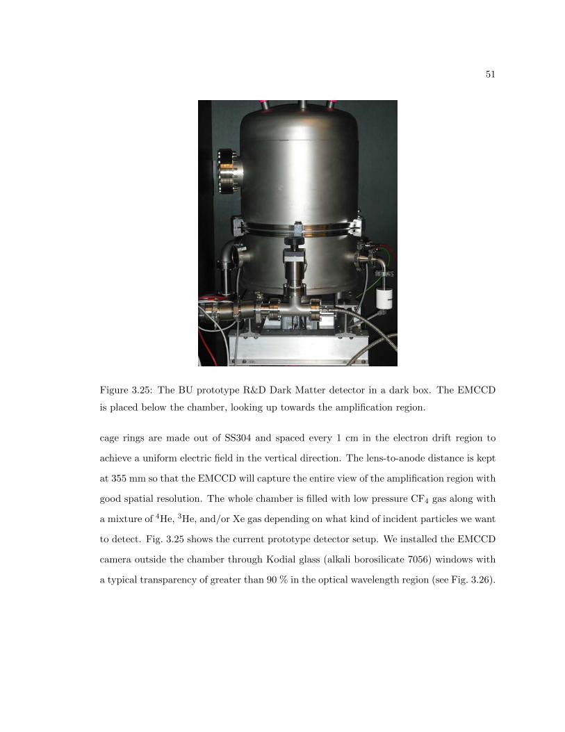
51
Figure 3.25: The BU prototype R&D Dark Matter detector in a dark box. The EMCCD
is placed below the chamber, looking up towards the amplification region.
cage rings are made out of SS304 and spaced every 1 cm in the electron drift region to
achieve a uniform electric field in the vertical direction. The lens-to-anode distance is kept
at 355 mm so that the EMCCD will capture the entire view of the amplification region with
good spatial resolution. The whole chamber is filled with low pressure CF4 gas along with
a mixture of 4He, 3He, and/or Xe gas depending on what kind of incident particles we want
to detect. Fig. 3.25 shows the current prototype detector setup. We installed the EMCCD
camera outside the chamber through Kodial glass (alkali borosilicate 7056) windows with
a typical transparency of greater than 90 % in the optical wavelength region (see Fig. 3.26).

52
Figure 3.26: The transmission spectrum of the Kodial glass window (Kurt J. Lesker Com-
pany).

Chapter 4
Fast-Neutron Tests with Prototype DM
Detector at MIT
4.1 Fast Neutron Detection from 252Cf
4.1.1 Introduction to 252Cf Neutron Runs
During the summer of 2008, after we began exploiting the advanced technology of the
EMCCD, we temporarily moved our Boston University prototype Dark Matter detector to
the Nuclear Reactor Laboratory Building NW13 at Massachusetts Institute of Technology
in order to do several tests with fast neutrons from a 252Cf fission neutron source and a
D+T neutron generator. Unfortunately, the use of the PMT was still under development,
so the data we obtained at MIT was only from the EMCCD with no PMT information for
the 3D reconstruction of the particle tracks.
The 252Cf neutron source (see Fig. 4.1(a)) at MIT has an activity of 3 mCi, which is roughly
108 Bq of nuclear reaction. Fig. 4.1(b) shows its typical neutron energy spectrum. Out of
those reactions, about 3 % goes into the fission reaction, and at each reaction there should
be 3.8 neutrons emitted. Thus, the number of fast neutrons emitted from this 252Cf neu-
tron source is the order of 107 neutrons per second in all directions. The efficiency of the
fast neutron interaction with 40 torr of CF4 gas inside the chamber is approximately 0.1 %,
53
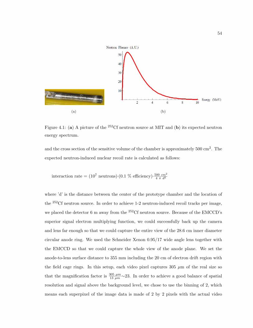
54
(a) (b)
Figure 4.1: (a) A picture of the 252Cf neutron source at MIT and (b) its expected neutron
energy spectrum.
and the cross section of the sensitive volume of the chamber is approximately 500 cm2. The
expected neutron-induced nuclear recoil rate is calculated as follows:
interaction rate = (107 neutrons)·(0.1 % efficiency)·500 cm2
4 π d2
where ’d’ is the distance between the center of the prototype chamber and the location of
the 252Cf neutron source. In order to achieve 1-2 neutron-induced recoil tracks per image,
we placed the detector 6 m away from the 252Cf neutron source. Because of the EMCCD’s
superior signal electron multiplying function, we could successfully back up the camera
and lens far enough so that we could capture the entire view of the 28.6 cm inner diameter
circular anode ring. We used the Schneider Xenon 0.95/17 wide angle lens together with
the EMCCD so that we could capture the whole view of the anode plane. We set the
anode-to-lens surface distance to 355 mm including the 20 cm of electron drift region with
the field cage rings. In this setup, each video pixel captures 305 µm of the real size so
that the magnification factor is 305 µm13 µm ∼23. In order to achieve a good balance of spatial
resolution and signal above the background level, we chose to use the binning of 2, which
means each superpixel of the image data is made of 2 by 2 pixels with the actual video

55
superpixels of the size 610 µm by 610 µm of spatial resolution.
4.1.2 252Cf Run Data with Pure CF4 Gas in BU Prototype
When high voltages were turned on for the anode and cathode (+620 v for anode and
-2500 v for cathode) and the detector was filled with 40 torr CF4 gas, the typical sparking
frequency without any radioactive source nearby was on the order of 0.1 Hz, although this
depended on the gas age. This means a single spark occurred every 1000 seconds. We be-
lieve sparks were caused in the amplification region. The heavy ions deposit lots of energy
and cause discharge events in the electric field region. When the 252Cf neutron source was
introduced into the room, even though it was sitting inside the moderator, the spark event
of the detector increased dramatically. The 252Cf source was placed into the cavity of the
housing made with Ricorad (2 % Borated Polyethylene with density of 0.945 g/cm3) neu-
tron absorber boards with a 2 cm by 2 cm opening directed towards the prototype detector.
Fig. 4.2 represents 30880 charged particle tracks (red markers) from the 252Cf run and
50 tracks of 241Am α particles (blue markers), both in the 40 torr CF4 gas detector, and
Fig. 4.3 presents the SRIM simulation of predicted ion/recoil tracks. One can see a band
of charge one protons at the bottom of the scatter plot. Those protons originated from
the field cage’s plastic spacers. Plastic contains quite a bit of hydrogen, which has a large
cross section with fast neutrons. The clump at the left bottom is from heavy nuclei recoils
induced by 252Cf fast neutrons with a typical energy of 1-2 MeV. It is very difficult to
separate fluorine from carbon. Among the data, only 4.44 % of all tracks identified are
unable to provide directionality information due to the small ratio of track length to track
width. Either the energy transferred from those recoils was too low, or the track had a
large electron drift distance. The x-axis is the projected length in cm captured by the
EMCCD camera. This was our very first detector experiment using a fast neutron source,
and at this point we did not have the PMT triggering/signaling ability together with the

56
Figure 4.2: A scatter plot of 252Cf fast-neutron-induced particle recoil tracks in a pure
40 torr CF4 gas.
Figure 4.3: A SRIM simulation of the recoil ranges in a pure 40 torr CF4 gas.

57
EMCCD. The data taking was missing a triggering system to prompt the EMCCD camera,
and we could not obtain the vertical component of any particle tracks. Thus, the exposure
time was set to 1 second continuously, and each frame was triggered internally at equal
frequency. The total real time of this run was 28.22 hours (101580 seconds), and the actual
live time was 20.38 hours (73366 seconds). Among the 73366 files recorded in this run, only
32137 images were identified as ’images with feature’. 343 files were categorized as ’sparks’;
once the 252Cf neutron source was introduced into the room where the chamber was, the
spark rate increased. This was because the increased number of neutrons induced heavy
ions to bump around the amplification region of the prototype chamber, and unfortunately
there was nothing we could do to avoid those types of spark events. Also, once the spark
occurs, the power supply is turned off due to its safety design, and it would take 6 seconds
to have it back on to the desired voltage value; thus, we had to reject any file recorded
within 6 seconds after each spark event. In this data set, 39521 files were categorized
as ’empty’. The empty images could contain very dim or low energy particle tracks, but
those were below the threshold level, and we could obtain no useful information from them.
Fig. 4.4 is an example of an identified particle track in 40 torr CF4 gas, induced by the
252Cf source’s fast neutrons. The energy threshold for the recoil recognition for this run
was ∼30 keV with the capability of recognizing the direction of the nuclear recoil. Fig. 4.5
is the examples of the 252Cf-neutron-induced nuclear recoil tracks including such low en-
ergy recoils captured by the EMCCD camera. Those images are in the series of order of
the track recognition from the beginning of the data taking. The direction of the neutrons
coming into the detector is from the image’s top to bottom. Because the energies of the
recoils are much less than a Bragg peak, the energy loss per unit length (dE/dx) or en-
ergy deposit should decrease as the recoil travels. This gives a clear idea of the moving
direction of the recoils captured. Those recoils moving upward (towards the Cf source) are
most likely induced by the neutrons that passed once through the detector, bounced back
from the wall, reentered the detector, and caused elastic scatterings with the nuclei of the

58
Figure 4.4: A typical 252Cf-neutron-induced nuclear recoil track in the prototype detector
of pure 40 torr CF4 gas. The view is roughly 30 cm by 30 cm. The 252Cf neutron source
was placed 6 m above the view; thus, the neutrons are coming from the top of the image.
The unit in the scale on the right is ADU. Particle track analysis program was integrated
by Andrew Inglis (Inglis, 2008).

59
Figure 4.5: Magnified images of 252Cf-neutron-induced nuclear recoil track in the prototype
detector of pure 40 torr CF4 gas. The energies of the recoil in the above images vary from
a few tens of keV (a few millimeters long) to several hundreds of keV (about a centimeter
long). A Gaussian filter is applied to those track images for visual integrity.
gas.
4.1.3 Electron Diffusion Check in 40 torr CF4 Gas
One important confirmation that had to be done along with the neutron experiment in the
this setting was to verify the expected amount of electron diffusion of the particle tracks
at various drift lengths in the exact setting and especially at 40 torr of CF4 gas pressure.
In order to carry out this experiment, I used three different americium α particle sources
at different drift lengths: 10 cm, 19 cm, and 2 cm from the amplification region, starting
from the left in Fig. 4.6(a).

60
(a) (b)
Figure 4.6: (a) A sample image of the α particle tracks with the electron drift distances
of 10 cm, 19 cm, and 2 cm respectively from left to right. (b) A CCD view of the whole
amplification region of the detector.
Taking the average of 100 images each of such α tracks per drift distance and applying
the Gaussian fit in the transverse direction to them as shown in Fig. 4.7(a); I obtained the
diffusion value for the three different electron drift lengths in a pure 40 torr CF4 gas (see
Fig. 4.7(b)).
The result of the diffusion measurement matched closely to the predicted values in 40 torr
CF4, even though we chose to use the binning function (each bin corresponds to 610 µm
by 610 µm) at the sacrifice of some spatial resolution.

61
(a) (b)
Figure 4.7: (a) An example of the Gaussian fit applied to the transverse diffusion of the
α particle tracks. (b) The electron diffusion value squared vs. the drift distance in a pure
40 torr CF4 gas. I have verified that the diffusion value is within our expectation in this
particular setting.
4.1.4 252Cf Run Data with Gas Mixture of CF4 and 4He in BU Prototype
After finishing the first 252Cf neutron run with the 40 torr CF4 gas detector, we also carried
out another experiment with a 40 torr CF4 and 600 torr 4He gas mixture. This is because
4He atoms have much greater cross section with neutrons on the order of an MeV, and as
a crucial part of our project, we needed to understand the capability of our detector as a
direction-sensitive neutron detector. Not only is the 4He cross section with high energy
neutrons in the MeV range high, but also the addition of 4He gas into 40 torr CF4 gas does
not change much of the scintillation or sparking characteristics of the detector. It is un-
avoidable that the electron diffusion and drift velocity in this gas mixture would increase;
however, most of the neutron interaction that would be useful to neutron detection come
from interactions with 4He atoms, and those ionized 4He atoms from the collision have
much greater range. Therefore, detecting the head-tail directionality of the particle recoil
tracks would not be a difficult task.

62
For this mixed-gas experiment, the anode and cathode voltages used were kept at the
same level as in the previous 40 torr CF4 detector’s case, +620 v and -2500 v respectively.
Adding 600 torr of 4He gas increased the neutron interaction efficiency from 0.1 % to 0.5 %
or greater, so in a very simple estimation we would expect several helium recoil tracks in
each image frame from this run. Fig. 4.8 shows the result of this run. The red markers
are the 252Cf -induced nuclear recoils, and the blue are the americium α particles as a
calibration source, and Fig. 4.9 is the SRIM simulation. Fig. 4.10 shows an example image
of the mixed gas run, and Fig. 4.11 shows the magnified images of recoil tracks from this
run. Compared to the previous run with pure CF4 gas, it is obvious that most of the re-
coils are helium nuclei with a charge of two. Because of this, the ambiguity of the particle
directionality in the data is as low as 0.75 %. This means the directionality detection failed
only 0.75 % of the time. This is better than the pure CF4 gas case by a factor of about 6.
4.1.5 Electron Diffusion Check in Gas Mixture of 40 torr CF4 and 4He
Most of the particle recoils in this gas mixture have a recorded projected length of greater
than 1 cm. The electron diffusion in this gas mixture is actually not too bad (see Fig. 4.12)
when compared to the pure CF4 case; the diffusion in the 4He gas mixture turned out to
be only about a 5 % larger from the pure CF4 electron diffusion. Although there is no
suggested electron diffusion value for this specific gas mixture of 40 torr CF4 and 600 torr
4He, our experimental result of very little increase in the electron diffusion compared to
the pure CF4 gas case is a very strong motivation to use this gas mixture for our neutron
detector.
4.1.6 Directionality Capability of our Detector
Another very important outcome from this fast neutron run was to quantify our detector’s
angular resolution capability and prove that our detector, with the mixture of 4He gas,

63
Figure 4.8: A scatter plot of 252Cf fast-neutron-induced particle recoil tracks in a gas
mixture of 40 torr CF4 and 600 torr 4He.
Figure 4.9: A SRIM simulation of the recoil ranges in a gas mixture of 40 torr CF4 and
600 torr 4He.

64
Figure 4.10: A typical Cf-neutron-induced nuclear recoil track in the prototype detector
of the gas mixture of 40 torr CF4 and 600 torr 4He. The view is roughly 30 cm by 30 cm.
The Cf neutron source was placed 6 m above the view; thus, the neutrons are coming from
the top of the image. The unit in the scale on the right is ADU.

65
Figure 4.11: Magnified images of 252Cf-neutron-induced nuclear recoil track in the proto-
type detector of the gas mixture of 40 torr CF4 and 600 torr 4He. The typical energies of
the helium recoils in the above images are on the order of several hundreds of keV (about
a centimeter long). A few tens of keV energy fluorine or carbon nuclear recoils are still
included with the similar rate as before. A Gaussian filter is applied to those track images
for visual integrity.

66
(a) (b)
Figure 4.12: (a) An example of the Gaussian fit applied to the transverse diffusion of the
α particle tracks. (b) The electron diffusion value squared vs. the drift distance in the gas
mixture of 40 torr CF4 and 600 torr 4He.
could be used as an efficient neutron detector with a good sense of directionality. The
detector, filled with a mixture of 40 torr CF4 and 600 torr 4He gas, was placed 6 m away
from the 252Cf neutron source. A schematic of the laboratory facility is shown in Fig. 4.13.
The room was surrounded by thick concrete walls on all sides, with the exception of a
hole to the neighboring room where an accelerator is placed. Another notable feature of
the room is the 24” thick concrete door that separates the neutron control room from this
laboratory space. There was no neutron moderating material around the detector in the
room, except the housing made with Ricorad that contains the 252Cf neutron source and
aims it in the direction of the detector.
The graphs in Fig. 4.14 show the angular distribution of the recoil helium nuclei, induced
by high energy neutrons from the 252Cf source sitting 6 m away from the detector. The
approximate angular resolution is about 10 and, most importantly, one can observe the
features in the room by looking at the angular distribution of the recoil tracks. At about
30, the neutron flux plateaus because the number of neutrons bouncing off the right wall

67
Figure 4.13: A sketch of the nuclear physics basement laboratory in the building NW-13
at MIT. The detector (blue) was placed inside a dark box, and the 252Cf neutron source
was placed at distance of 6 m away (yellow).

68
(a)
(b)
Figure 4.14: (a) The angular distribution of the 252Cf-neutron-induced nuclear recoil tracks
in the gas mixture of 40 torr CF4 and 600 torr 4He. (b) The energy of the 4He recoil in
the added axis in the 3D plot (Inglis and Hartwig, 2008). This shows that the flux of 4He
recoils with higher energy is at maximum in the direction pointing towards the 252Cf fission
neutron source.

69
coming into the chamber decreases. Exactly at 90, which is the direction of the 252Cf
neutron source, the neutron flux reaches its maximum. Around 220-230, the flux is at a
local maximum; this is due to the neutrons bouncing back from the concrete wall located
at this angle from the detector. Then at 270, which is exactly the opposite direction of
where the 252Cf source is located, is the second greatest peak. This peak is due to the
neutrons passing through the detector once without interacting, then get bounced off the
wall behind, coming back into the chamber and inducing the helium recoil. The detector,
filled with just pure 40 torr of CF4 gas, also has the capacity of the directionality; however,
when the detector should be used specifically as a direction-sensitive neutron detector, en-
ergy and momentum transfer onto helium nuclei is much more efficient than relying merely
on the heavier nuclear recoils such as carbon or fluorine. This result confirms the great
potential of our detector as a direction-collimatorsensitive fast neutron detector. Fig. 4.15
shows the angular distribution result from a pure CF4 detector with the use of the 252Cf
neutron source in the similar fashion. Although the pointing capability of the detector
can offer very good directionality without the addition of any 4He gas, the typical angular
resolution goes as high as 25 %, and the capability of distinguishing minor detail such as
the location of objects in the room would be lost.
4.2 Fast Neutron Detection from D+T Neutron Generator
at MIT
4.2.1 Introduction to D+T Neutron Generator Neutron Runs
Another fast neutron source device we used at the MIT nuclear physics laboratory is a
Thermo Scientific D+T neutron generator model A-325 (see Fig. 4.16). The neutron rate
in the company’s specification is listed as ”<108 (n/s)”, and when we took a measurement
in summer 2008, the actual flux came out as ∼6.2×10³ (/s/cm2)±5 % measured at 26 cm.
This is about 5×10⁷ (/s) emitted, which agrees with the specification value. The typical

70
Figure 4.15: The angular distribution of the Cf-neutron-induced nuclear recoil tracks in a
pure 40 torr CF4 gas as a comparison. Although the directionality information is still very
useful, the angular resolution is not nearly as good as the other gas mixture case.
Figure 4.16: The image of the D+T neutron generator from Thermo Scientific (Thermo
Scientific).

71
energy of neutrons created in this generator is 14.1 MeV by the fusion reaction of Deuteron
and Triton. The number of neutrons emitted from this neutron generator is roughly 5 times
more than that of the 252Cf source we used in our previous experiment. When the energy
of neutrons is on the order of an MeV, which is the case of 252Cf neutrons, the majority
of the interactions with either the carbon or fluorine of the CF4 gas is elastic collisions.
However, as the energy of neutrons increase, the number of inelastic collisions of carbon
or fluorine atoms becomes non-negligible, and at 14.1 MeV of neutron energy, quite a few
inelastic interactions occur.
Fig. 4.17(a) and Fig. 4.17(b) represent the neutron cross section with carbon and fluorine
atoms. In both cases, the blue lines correspond to the total interaction, and the green lines
are the elastic interactions. One can see that at typical 252Cf neutron energy at 1-2 MeV,
the cross section is dominated by elastic collisions. At the neutron energy of 14.1 MeV, two
kinds of inelastic interactions with carbon atoms frequently occur: one is that a neutron
breaks a carbon atom into beryllium and an α particle (presented in red color), and the
other is a carbon breaks into three α particles (presented in light blue color). In fluorine’s
case, most of the inelastic collisions lead to either the creation of oxygen and a proton (pre-
sented in black and pink colors), or nitrogen and an α particle (presented in red and light
blue colors) pairs. The nuclear recoil energy from the elastic collisions of course increases
compared to the ones from the 252Cf neutrons. A majority of the elastic nuclear recoils
would have energy greater than an MeV with typical ranges of several centimeters.
4.2.2 D+T Neutron Generator Run Data with Pure CF4 Gas in BU
Prototype
Fig. 4.18 shows the elastic and inelastic interactions for 14.1 MeV neutrons incident on
CF4. Fig. 4.19 shows some examples of high-energy recoils from elastic collisions, and
Fig. 4.20 shows examples of inelastic collision events. Many of the inelastic collisions result
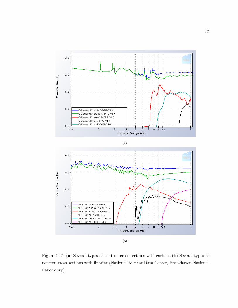
72
(a)
(b)
Figure 4.17: (a) Several types of neutron cross sections with carbon. (b) Several types of
neutron cross sections with fluorine (National Nuclear Data Center, Brookhaven National
Laboratory).

73
Figure 4.18: 14.1 MeV-neutron-induced nuclear recoil tracks in the prototype detector of
pure 40 torr CF4 gas. Both inelastic and elastic recoil are seen in this image. The view is
roughly 30 cm by 30 cm. The neutron generator was placed 6 m above the view; thus, the
neutrons are coming from the top of the image. The unit in the scale on the right is ADU.

74
Figure 4.19: Magnified images of the elastic nuclear recoil tracks induced by the 14.1 MeV
neutrons in the prototype detector of a pure 40 torr CF4 gas. The energies of the recoils
vary from as low as several tens of keV (a few millimeters long) to the order of MeV (several
centimeters long). A Gaussian filter is applied to those track images for visual integrity.
Figure 4.20: Magnified images of the inelastic nuclear recoil tracks induced by 14.1 MeV
neutrons in the prototype detector of a pure 40 torr CF4 gas. The track length can vary
up from >20 cm down to less than a centimeter depending on the transferred energy. A
Gaussian filter is applied to those track images for visual integrity.

75
Figure 4.21: The scatter plot from the pure 40 torr CF4 gas setup with the neutron sources:
252Cf (red) and the 14.1 MeV neutron generator (green). Each data set contains exactly
5,000 unbiased particle tracks found by the track recognition computer program.
in two particle outcomes, which can be predicted with the neutron cross section data (see
Fig. 4.17(a) and Fig. 4.17(b)). Fig. 4.21 compares the 5,000 particle tracks from the 252Cf
and neutron generator runs with the pure 40 torr of CF4 gas.
The scatter plot in Fig. 4.21 contains; (1) charge-one proton tracks mainly due to the
neutron collisions with the plastic material inside the chamber, (2) naturally occurring
background α particles from the inside material, (3) nuclear elastic collisions, and (4) nu-
clear inelastic collisions of the gas atoms. The charge-one proton band from the plastic
material inside the detector is identical in the two runs. The elastic nuclear collision events

76
Figure 4.22: The numbers of events in the scatter plot (see Fig. 4.21). The α background
events are counted only in the 252Cf data, and I used the same rate for the neutron generator
run as well.
also make a local cluster, which agrees in both cases. Those elastic nuclear recoils induced
by higher energy neutrons (green markers in Fig. 4.21) from the neutron generator form a
longer band of the cluster. The table in Fig. 4.22 shows the number of each type of event
contained within the sample of the 5000 particle tracks in each run. After subtracting all
interactions but the inelastic events, the rate of the inelastic collision events in the 252Cf
run was 0.36 %, and in the neutron generator run was 14.8 %.
Because fluorine atoms constitute 80 % of the CF4 gas, and fluorine’s neutron cross section
is much higher in most of the 252Cf neutron energy spectrum, the majority of the inelastic
events are due to the fluorine recoils. In order to verify the accuracy of our data, I used
the expected neutron cross section information from the National Nuclear Data Center
(National Nuclear Data Center, Brookhaven National Laboratory) and made an estimate
of the inelastic collision events rate for a 40 torr CF4 gas. Fig. 4.23 shows the neutron
cross sections of carbon and fluorine atoms. Blue markers correspond to the total cross
section, the green markers are for the exact 14.1 MeV neutron generator neutrons inelastic
cross sections, and the red markers describe the inelastic cross sections from a 252Cf with
the typical neutron energy spectra correction (see Fig. 4.1).
After integrating all the appropriate energy spectrums of the incoming 252Cf neutrons, I

77
(a)
(b)
Figure 4.23: The interaction probability plots for carbon (a) and fluorine (b) atoms. Blue
markers represent the total interaction. The green markers correspond to the probability
of interaction with the neutron-generator neutrons (14.1 MeV only), and the red markers
stand for the interaction probability with the 252Cf neutrons (the californium neutron
energy spectrum has been taken into consideration in this estimation). The probability
(y-axis) is in an arbitrary unit.

78
Figure 4.24: Magnified images of the three-α interaction candidates induced by 14.1 MeV
neutrons in the prototype detector of a pure 40 torr CF4 gas. The track length can vary
up from >20 cm down to less than a centimeter depending on the transferred energy. A
Gaussian filter is applied to those track images for visual integrity.
obtained the inelastic collision event rate of 0.385 % for a 252Cf and 16.1 % for a neutron
generator neutron sources. Although an energy resolution was as bad as 20 %, the pro-
totype Dark Matter detector demonstrated an extraordinary detection capability for both
elastic and inelastic neutron collision events. On rare occasions, one can also find three
pronged tracks which are clear candidates for three α particle production (see Fig. 4.24).
The precise energy measurements on each track of those events are extremely difficult and
still underway, and we may need much higher energy resolution for a good study of such
events in our detector as well. There is still room for improvement in increasing the energy
resolution of this detector for much more sensitive and accurate recoil energy measurements
in the next generation DMTPC Dark Matter detector.
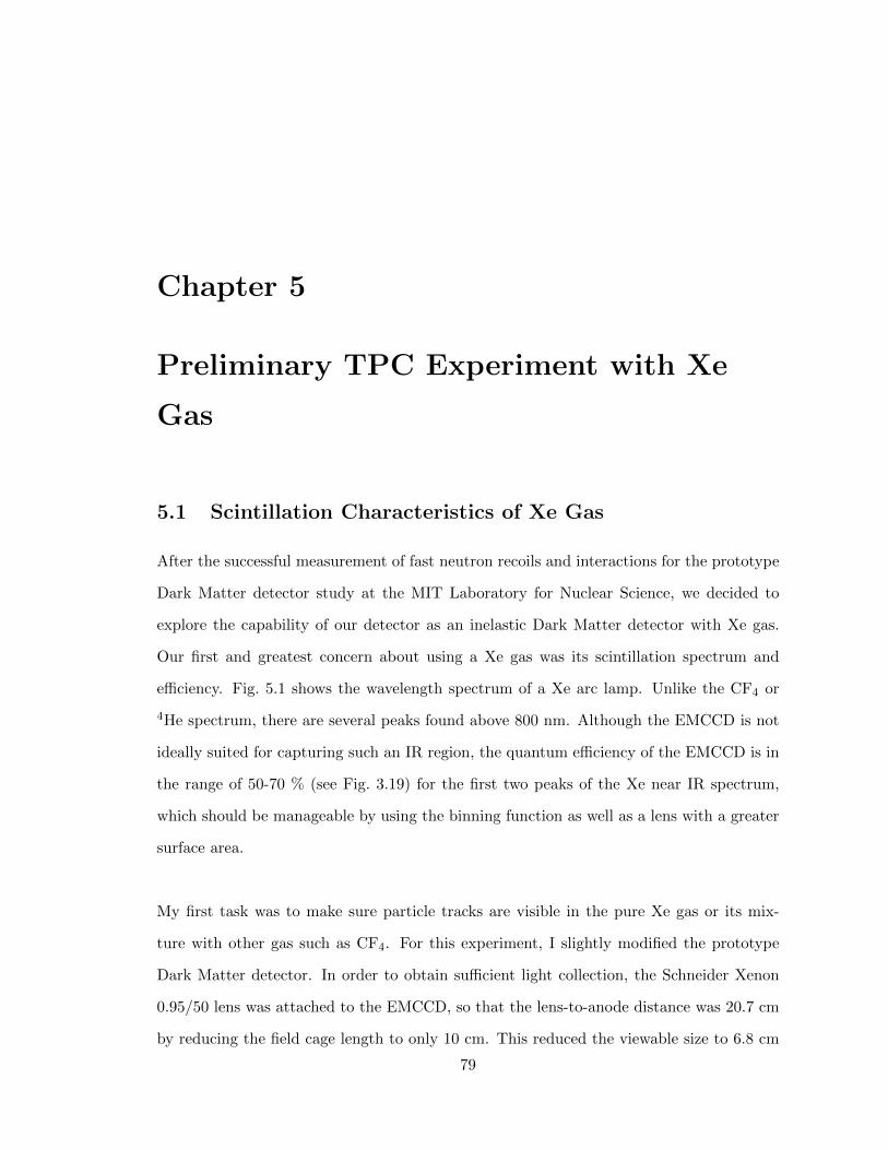
Chapter 5
Preliminary TPC Experiment with Xe
Gas
5.1 Scintillation Characteristics of Xe Gas
After the successful measurement of fast neutron recoils and interactions for the prototype
Dark Matter detector study at the MIT Laboratory for Nuclear Science, we decided to
explore the capability of our detector as an inelastic Dark Matter detector with Xe gas.
Our first and greatest concern about using a Xe gas was its scintillation spectrum and
efficiency. Fig. 5.1 shows the wavelength spectrum of a Xe arc lamp. Unlike the CF4 or
4He spectrum, there are several peaks found above 800 nm. Although the EMCCD is not
ideally suited for capturing such an IR region, the quantum efficiency of the EMCCD is in
the range of 50-70 % (see Fig. 3.19) for the first two peaks of the Xe near IR spectrum,
which should be manageable by using the binning function as well as a lens with a greater
surface area.
My first task was to make sure particle tracks are visible in the pure Xe gas or its mix-
ture with other gas such as CF4. For this experiment, I slightly modified the prototype
Dark Matter detector. In order to obtain sufficient light collection, the Schneider Xenon
0.95/50 lens was attached to the EMCCD, so that the lens-to-anode distance was 20.7 cm
by reducing the field cage length to only 10 cm. This reduced the viewable size to 6.8 cm
79
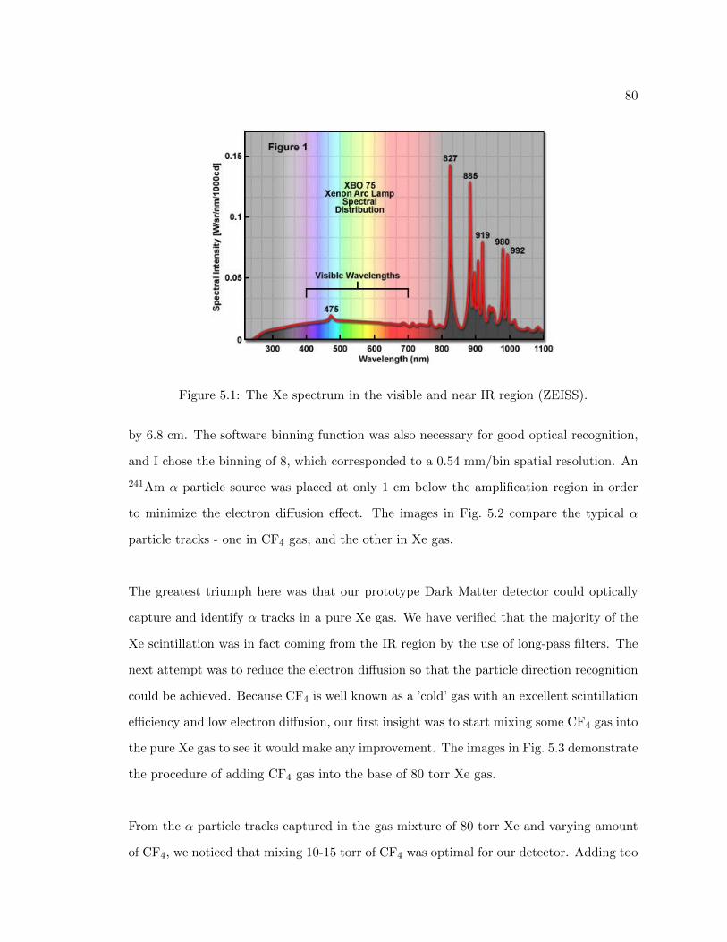
80
Figure 5.1: The Xe spectrum in the visible and near IR region (ZEISS).
by 6.8 cm. The software binning function was also necessary for good optical recognition,
and I chose the binning of 8, which corresponded to a 0.54 mm/bin spatial resolution. An
241Am α particle source was placed at only 1 cm below the amplification region in order
to minimize the electron diffusion effect. The images in Fig. 5.2 compare the typical α
particle tracks - one in CF4 gas, and the other in Xe gas.
The greatest triumph here was that our prototype Dark Matter detector could optically
capture and identify α tracks in a pure Xe gas. We have verified that the majority of the
Xe scintillation was in fact coming from the IR region by the use of long-pass filters. The
next attempt was to reduce the electron diffusion so that the particle direction recognition
could be achieved. Because CF4 is well known as a ’cold’ gas with an excellent scintillation
efficiency and low electron diffusion, our first insight was to start mixing some CF4 gas into
the pure Xe gas to see it would make any improvement. The images in Fig. 5.3 demonstrate
the procedure of adding CF4 gas into the base of 80 torr Xe gas.
From the α particle tracks captured in the gas mixture of 80 torr Xe and varying amount
of CF4, we noticed that mixing 10-15 torr of CF4 was optimal for our detector. Adding too

81
(a) (b)
Figure 5.2: α particle tracks captured in the central 6.8 cm by 6.8 cm region of the prototype
Dark Matter detector in (a) 40 torr CF4 gas and (b) 80 torr Xe gas. The electron diffusion
values are 0.35 mm and 6.8 mm relatively. The electron diffusion value at the drift distance
of 1 cm in the 40 torr CF4 gas fully agrees with the suggested/observed value (see Fig. 4.7).
The applied amplification voltages were +620 v and +415 v respectively.

82
Figure 5.3: The α particle tracks captured in the central 6.8 cm by 6.8 cm region of
the prototype Dark Matter detector. The gas basis was the pure 80 torr Xe with various
admixtures of CF4 gas. The amount of CF4 gas added in torr and the applied amplification
voltage in volts are as follows: (PCF4, VAnode) = (0, 415), (1, 430), (5, 470), (10, 500), (15,
525), (20, 550), (25, 570), and (30, 590) respectively from the top-left down to bottom-right.
The amplification voltage was set to the highest possible without any sparking.

83
much CF4 quenched the scintillation efficiency. With the 10 torr and 15 torr CF4 mixture,
the electron diffusion σ values were 1.1 mm and 0.7 mm respectively. Low energy Xe recoils
from an inelastic collision off a Dark Matter particle with a typical energy of tens of keV
would travel less than a millimeter in such a gas mixture. Thus, although our detection
method with the gas mixture of Xe and CF4 would work beautifully in the inelastic Dark
Matter search, no directionality information could be obtained.
5.2 Non-Linearity of the Stopping Power of Xe Gas
Another interesting feature of Xe gas we discovered was the non-linear relationship of the
moving ion’s scintillation quantity and the amount of energy lost per unit length (dE/dx).
In CF4, there is a clear linear relationship between the scintillation energy and dE/dx (see
Fig. 2.4); thus, it is very easy to predict the amount of the stopping power by a linear
factor. If the scintillation efficiency of Xe gas changes in a non-linear fashion, we could
exploit this unique attribute to make the detector background free. For this study, I have
set the gas pressure to the successful gas mixture of 80 torr Xe and 10 torr CF4 as seen in
Fig. 5.3. The six images in Fig. 5.4 display the change in the scintillation by the applied
amplification voltages. Roughly 2.5 MeV of the α energy is contained in each viewable
frame.
In order to quantify this non-linearity, I extracted the light level of the α tracks at each
centimeter from the Bragg peak and made comparisons at different anode voltages (see
Fig. 5.5). Fig. 5.6 illustrates the ratio of the scintillation level (measured in ADU) to that
of the Bragg peak value vs. the location of the measurement along each α track at every
centimeter. The dE/dx curve is presented in a purple dotted line, predicted by the SRIM
simulation. Unlike the linear relationship between the light emission vs. dE/dx of the CF4
gas (see Fig. 2.4), Xe gas shows very strong non-linear characteristics. The above result
also confirms that the rate discrepancy of the scintillation level and the stopping power

84
Figure 5.4: The α particle tracks captured in the central 6.8 cm by 6.8 cm region of the
prototype Dark Matter detector. The gas mixture was 80 torr Xe and 10 torr CF4. The
applied amplification (anode) voltages in volts were 495 v, 490 v, 480 v, 470 v, 460 v, and
450 v respectively from the top-left down to bottom-right.
Figure 5.5: An α particle track in the gas mixture of 80 torr Xe and 10 torr CF4. The α
was moving from the right to left, going through its Bragg peak right before it came to
rest. For the comparison study of the scintillation vs. dE/dx, I took the scintillation ratio
at each cm to the Bragg peak value.

85
Figure 5.6: The amplification voltages have been varied for the study of the scintillation
vs. dE/dx. This plot shows the ratio of the scintillation level to the Bragg peak vs. the
distance from the Bragg peak. The purple dotted line is from the SRIM simulation. This
shows that the scintillation energy is highly non-linear to the stopping power or dE/dx in
Xe gas.

86
was strongly emphasized as the amplification voltage increased. This means that the de-
tection threshold can be cleanly and manually controlled by the amplification voltage so
that the Dark Matter-induced nuclear recoil would trigger the system, where the typical
background noise such as beta or γ rays would be way below the threshold limit, and the
detector would be free from those backgrounds. In the future, we are certainly interested
in applying this idea to our inelastic Dark Matter search.

Chapter 6
Preparations for the Background Neutron
Detection Experiment
6.1 EMCCD and PMT Dual Readout System
After the preliminary study of the Xe gas application with our prototype Dark Matter
detector, we began improving it with the use of PMTs. The use of PMTs is beneficial in
two ways; first, we can use the signal from them as a trigger for the image capturing sys-
tem, and second, we can use them to obtain vertical information about the particle tracks.
The picture presented in Fig. 6.1(a) is the new image capturing system for our prototype
detector. The lens used was the Schneider Xenon 17/0.95 lens, mounted onto the EMCCD
via the C-mount. Six Hamamatsu R7400U-20 PMTs surround the lens - one is designated
for the trigger signal, and the remaining five are connected in a linear fan-in/out fashion
and used to record the PMT signal of the particle tracks. These PMT are made for use in
Visible to Near IR range, with enhanced quantum efficiency in the red region. The solid
red line in Fig. 6.1(b) represents the quantum efficiency of those tubes.
Prior to the use of the PMT as a trigger, we utilized the EMCCD camera in a single image
continuous exposure mode, which means that the exposure occurs continuously followed
by a complete flushing of the CCD chips in order to keep the image clean. Although it
operated well as a detector of particle recoils induced by neutrons when exposed to high
87

88
(a) (b)
Figure 6.1: (a) An EMCCD and PMT dual readout setup. The Schneider Xenon 0.95/17
lens (under the plastic cover) is surrounded by six Hamamatsu R7400U-20 red-sensitive
PMTs. (b) Hamamatsu PMT quantum efficiency (Hamamatsu).

89
rate neutron sources such as the 252Cf or neutron generator that we used at MIT, this mode
creates too much dead time and produces too many blank frames that contain no actual
particle track. Thus, from the particle track recognition point of view, it was necessary to
improve the PMT triggering system so we could operate the detector in a background run
without losing too much data storage space or coping with too much dead time.
In this setup, five PMTs were connected in parallel to add the PMT signals. Each PMT
has a light sensitive area of about 1 cm in diameter. Summing up the five tubes, the total
surface area became roughly 40 % of the Schneider 17 mm lens, making it possible to obtain
enough light from the particle tracks. The single PMT that was designated for a trigger
was connected directly to a preamplifier and amplifier (Ortec model 925-SCINT). Then
the pulse went through a discriminator to distinguish signal pulses from electronic noise
or spark events. Finally the signal went through a gate (LeCroy model 222 Dual Gate
Generator) to send a 1 µs width TTL signal to both EMCCD and oscilloscope. When
the EMCCD received this TTL signal, it began the image recording procedure for a pre-
designated exposure time as specified by the user. The TTL signal sent to an oscilloscope
was used as a trigger for the signal from the sum of the five PMTs. The digital oscilloscope
was a LeCroy Wavesurfer 452 which ran on a Windows operating system (see Fig. 3.2).
One of the main issues was the matching of the EMCCD image and PMT pulse signal for
each particle track. Although both the EMCCD and oscilloscope receive the same TTL
pulse, the data processing speed of each device varies and the number of PMT signals
saved is greater than that of the EMCCD images. This is because the computer that is
processing the EMCCD requires roughly half a second to be ready for the next exposure
in a continuous data saving mode.
In order to match the data files from EMCCD and PMT, we decided to use the time stamp
created by the operating system. For an accuracy of ±1 second or more, we connected a

90
Clock Watch Cell Sync device from Beagle Software to both computers. This device re-
ceives a time synchronization signal from the CDMA every second and synchronizes both
computers’ times. During the file-matching process, one of the most important criteria was
that two files’ (one from EMCCD, and the other from PMT) time stamps were less than
1 second apart and that there’s no other match within this ±1 second.
6.2 Two Experiments for the BU Prototype Chamber Quan-
tification
Before starting any data measurement with this new EMCCD and PMT dual system, I
carried out two experiments in order to better understand the sparking problems and EM-
CCD and PMT signal correlation techniques. One was to better understand why and when
discharge events happen in the amplification region and if there was a way to avoid such
events. The other was how to construct the previously missing vertical dimension data of
the particle tracks, which is now saved as a PMT data.
6.2.1 Spark Experiment
Sparking events in the amplification region have always been one of our greatest concerns.
In a typical amplification region, the spacing is the order of hundreds of micrometers, and
we would like to apply as much voltage as possible in order to achieve a high electron gain.
Stretching the mesh as well as we can is of course the number one priority. That being
given, the applicable voltage also varies depending on the pressure and type of gas used in
the detector. Thus, for any gas composition and pressure, we always seek the maximum
applicable voltage without constant sparking events. When the detector was subjected to
copious numbers of fast neutrons in the nuclear physics lab at MIT, the rate of sparking
jumped up. This suggests that there could be some sort of connection between the number
of heavy ions in the amplification region and the number of spark events. In order to verify
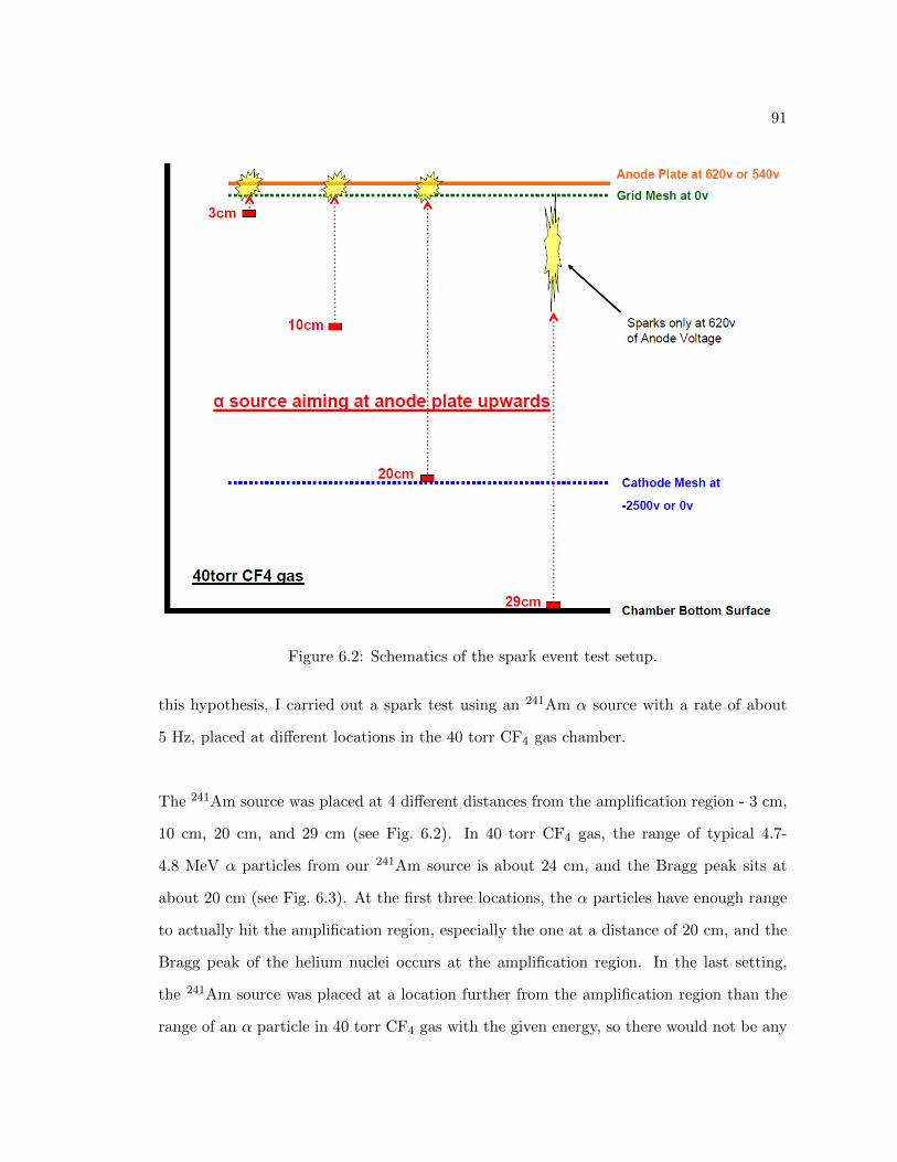
91
Figure 6.2: Schematics of the spark event test setup.
this hypothesis, I carried out a spark test using an 241Am α source with a rate of about
5 Hz, placed at different locations in the 40 torr CF4 gas chamber.
The 241Am source was placed at 4 different distances from the amplification region - 3 cm,
10 cm, 20 cm, and 29 cm (see Fig. 6.2). In 40 torr CF4 gas, the range of typical 4.7-
4.8 MeV α particles from our 241Am source is about 24 cm, and the Bragg peak sits at
about 20 cm (see Fig. 6.3). At the first three locations, the α particles have enough range
to actually hit the amplification region, especially the one at a distance of 20 cm, and the
Bragg peak of the helium nuclei occurs at the amplification region. In the last setting,
the 241Am source was placed at a location further from the amplification region than the
range of an α particle in 40 torr CF4 gas with the given energy, so there would not be any

92
Figure 6.3: The SRIM simulation of the typical 4.8 MeV energy α particle range in a
40 torr CF4 gas.
direct collision of the helium ion within the amplification region. However, the ionization
electrons from the path of the α particle are expected to reach some small local area of
the amplification region. For this spark experiment, I also used two different amplification
voltage setting, one is the standard detector running voltage of 620 V, with which we have
good electron gain for the scintillation with a manageable spark rate on the order of 0.1 %.
The other voltage setting I used for this experiment was 540 V, which is way below the
standard voltage we use for the chosen amplification spacing of 530 µm and almost never
causes a discharge event in the amplification region in normal conditions.
My underlying assumption for the causes of sparking events was a combination of heavy
ion and/or swarm of ionization electrons bombarding the intense electric field amplification
region. The first conclusion comes from the comparison of the spark rate when there is no
α source inside and when it is placed so that the α particles are emitted horizontally. At
the standard voltage of 620 V, the spark events occur at a typical rate of 0.1 Hz due to
the radioactive background of the material inside the chamber itself. This is unavoidable
unless one uses material that is low radioactive. When the 241Am was placed at 3 cm
below the amplification region with the horizontal emission of α particles, there was a very

93
Figure 6.4: The spark test data outcome. Values in the 2nd column, ”α Travel Distance,”
correspond to the α source location described in Fig. 6.2. ”100 %” means the spark event
always occurs. The other values (in %) correspond to rates in Hz.
slight increase of the spark rate. This is because the α particles’ angle of emission past the
collimator is about ±11, and with the range of αs being greater than 20 cm, some of the
α particles may end up entering the amplification region.
Secondly, this can be seen by comparing the spark rates of all settings at the voltage of
540 V (see 2nd and 3rd columns of Fig. 6.4). When the 241Am source was placed at distance
greater than the α particles’ range, the spark event was essentially negligible as much as
no source was introduced in the detector. However, for those settings where the distance
is less than the range of α particles (3 cm, 10 cm, or 20 cm), one can observe an increase
of the spark rate even at such a low voltage setting. This leads to the conclusion that
nuclei collision to the amplification region could easily trigger the discharge event. In the
comparison of the spark events in this column, we have also noticed that the spark rate
changes depending on the distance the α particles travel. On top of what we just discovered
above, we learned that it is not only the nuclei collision, but also its energy loss makes a
difference in the spark rate. With such a relatively low voltage, when the 241Am source

94
was placed at 20 cm of distance so that the Bragg peak occurs right at the amplification
region, the discharge or spark occurs continuously. This conclusion offers strong evidence
that the spark events are strongly correlated with how much energy is emitted by a moving
ion in the intense electric field region.
Thirdly, the 4th column in Fig. 6.4 (620 V of applied voltage) implies the strong involve-
ment of the ionization electrons in the spark events. At the standard voltage of 620 V,
the electric field in the amplification region is very intense in order to reach a good com-
bination of high electron gain and a manageable spark rate when there is no radioactive
source inside the chamber. At this voltage setting, the location of the 241Am source makes
no difference in the spark rate provided the α emission targeted towards the amplification
region. At a distance of 29 cm, there is no way the heavy helium ion could have reached
the amplification region; however, the spark events occurred continuously, which indicates
that the local swarm of ionization electrons can also trigger discharge events at the de-
tector’s regular running voltage settings. This is also backed up by the experiments listed
in the 5th column in Fig. 6.4, where the cathode voltage was turned off. In this column,
there is no drift electric field; thus, the ionization electrons from the particle tracks merely
drift around and do not cause any intense local electron bombardment in the amplification
region.
From this experiment, we learned more about the involvement of heavy ions and ionization
electron collisions in the intense electric field region. This experiment explains why the rate
of sparking jumped up when the fast neutron source was introduced into the detector. The
energetic neutrons continuously collide with the atoms of the material inside the chamber,
releasing copious numbers of heavy ions hitting the amplification region. Therefore, in the
process of chamber construction, it becomes very important to employ material that is
high in radiopurity in order to reduce the chance of sparks in standard detector running.
Using material with smooth surfaces and constructing mechanically superior amplification

95
systems contributes to making a good system with lower and almost negligible spark event
rate; however, it is impossible to reduce the rate to zero because of the involvement of ions
and electrons in the spark events mentioned in the above conclusions.
6.2.2 Correlation Experiment
Another small experiment that I have carried out was the analysis of the combined data
from the EMCCD and PMT. As previously stated, the 2D images of the CCD data only
give data of the projected particle tracks onto the amplification region. In order to recon-
struct the full 3D structure of the particle tracks, it is necessary to utilize the data obtained
by the PMT. For this experiment, I have used the same 241Am α sources used previously
but placed them in several different angles and directions, and analyzed the correlated data
set obtained by the EMCCD and PMT.
The 241Am α source was placed at either 3 cm or 17 cm away from the amplification re-
gion. At each location, the source was placed so that the angle of α particle emission with
respect to the amplification region took on three different values: 0 (horizontal), 45, and
60 (see Fig. 6.5). Those particles moving with an angle from the source placed at 3 cm
from the amplification region are moving away from the amplification region, and those
that are at 17 cm of distance from the amplification region, the α source was placed so
that α particles traveled towards the amplification region with angles. The objective of
this experiment was not only to learn about the correlation of the data sets, but also to
learn and verify the electron drift velocity in the 40 torr CF4 gas. The following are the
examples of correlated data of EMCCD particle track image and PMT pulse (see Fig. 6.6,
6.7, and 6.8). Time runs from the top to the bottom of the PMT signal view on the right
side. A green dot indicates the beginning of leading edge, and a yellow dot points to the
end of trailing edge of the pulse.

96
Figure 6.5: The setup for the PMT pulse study with an 241Am α source in a pure 40 torr
CF4 gas. Three angles of incident were chosen: 0 (horizontal), 45, and 60. For each
angle setup, the α particles were set moving both upward and downward.
(a) (b)
Figure 6.6: The horizontal α emissions with (a) 3 cm and (b) 17 cm electron drift distances.

97
(a) (b)
Figure 6.7: The 45 angle α emissions α emissions with (a) away from and (b) towards
the electron amplification region.
(a) (b)
Figure 6.8: The 60 angle α emissions α emissions with (a) away from and (b) towards
the electron amplification region.

98
The real size of the EMCCD view is the same as before - roughly 30 cm by 30 cm. On
the right side are the PMT signals recorded on the oscilloscope, and the time runs from
the top to the bottom of the view. The first two image sets show very fast signals from
the PMT (see Fig. 6.6). This is because the actual ion velocity is much greater than the
electron drift velocity, so when the α particles are travelling horizontally, the time we mea-
sure from the oscilloscope is the time it takes for the ion to travel before it comes to rest.
But in comparison to those horizontal particle motions, the angled particle tracks show
much longer pulses in the oscilloscope, which is due to the slower electron drift velocity.
As one can see from the images in Fig. 6.6, 6.7, and 6.8, another important aspect of the
PMT signal is that when the α particle is moving away from the amplification region,
the maximum pulse height occurs at the end of the light emission. When the particles
are moving towards the amplification region, this maximum pulse height happens at the
beginning of the pulse. This is due to the Bragg peak of the dE/dx and the timing of
when it happened. When the α particle is moving away from the amplification region,
most of the ionization electrons before the Bragg peak would already reach the amplifi-
cation region before those from the Bragg peak. On the other hand, when the α particle
is moving towards the amplification region, because the ion velocity is much faster than
the electron drift velocity, that greater swarm of electrons from the Bragg peak reaches
the amplification region before the electrons that were created at earlier times but are still
drifting through the gas to reach the amplification region. Fig. 6.9 is a scatter plot of
the projected track lengths in centimeters vs. PMT pulse widths which is multiplied by
the electron velocity, so that the units match. The electron drift velocity is discussed below.
In Fig. 6.9, the red and blue markers represent horizontal α particle tracks. Yellow and
black are for the 45 of emission, and light blue and light green are for the 60 angle of α
emissions. As in the previous experiment, the opening angle of the α emission through the
collimator is ±11. This uncertainty of the emission angle gives the width of each angle’s
band. The PMT width data recorded in each file is on the order of microsecond. Mul-

99
Figure 6.9: Red and blue markers are the horizontal a tracks with drift distances 3 cm and
17 cm respectively. Yellow and black markers are 45 angled a tracks with the starting
drift distance of 3 cm and 17 cm respectively. Light green and light blue markers are 60
angled a tracks with the starting drift distance of 3 cm and 17 cm respectively.

100
tiplying this number by the electron velocity, which is gas type and pressure dependent,
gives the particle’s vertical track length. Some of the angled particle tracks typically seem
to have shorter track lengths (especially the ones at a 60 angle moving away from the
amplification region). This is due to the collimator material’s disturbance of the electron
path. In this experiment, I used an aperture of 20 µm in diameter at the center of circular
structure of 30 mm in diameter. Thus, when the emission is tilted to an angle of θ, the first
’15 mm· sin θ’ of the particle track is blocked by the collimator itself. Also, compared to
when the α particle source is placed at 17 cm from the amplification region (which is closer
to the EMCCD camera), when placed at 3 cm location, the collimator stands between the
amplification region and lens and blocks the scintillation path more noticeably; thus, it
makes the tracks length seem shorter than the other cases. While attempting to acquire
the electron drift velocity, I needed to take this effect into consideration. Once that was
done, I looked for the drift velocity coefficient that makes the α particle track length, which
is obtained by the square-root of projected length squared plus vertical length squared, the
most uniform for any α emission angle by making the best fit for it. By doing so, I have
concluded that the electron drift velocity is ∼11 cm/µs in 40 torr CF4 gas. This outcome
agrees with the suggested value of electron drift velocity suggested by Christophorou et al
(Christophorou et al., 1996). In any gas combination for this detector, it is crucial to know
the electron drift velocity for reconstructing the full 3D particle track information.
6.2.3 Electron Diffusion Effect on EMCCD Readout
From this experiment, I also obtained the information necessary to quantify how the elec-
tron drift distance affected the total energy recognized by the particle track finding pro-
gram. As electrons drift in the field cage’s drift region, the particle tracks lose their energy
intensity because the light intensity of the edge of the particles goes below EMCCD’s
background level. Determining the boundary between particle tracks and background level
depends solely on the parameters (Gaussian blur and threshold values) we use when run-

101
ning through the data. When a particle track occurs close to the amplification stage, and
the electrons have very little distance to travel before reaching the grid mesh, the total
energy of the particle track recognized by the computer program becomes higher than the
case when a particle track occurs far away from the amplification region (see Fig.6.6). This
effect is unavoidable in the optical-TPC technique we use with an EMCCD (or a regular
CCD) camera. Fig. 6.10 compares the typical projected range vs. energy distribution of an
241Am α particles traveling horizontally with an electron drift distance of 3 cm and 17 cm
measured by the EMCCD (see Fig.6.5 for the detailed setup). Compared to the energy
deposited recognized for the 3 cm of electron drift distance case, the 17 cm drift distance
shows approximately 18 % less energy recognized for the same range of α particles. As
I explained earlier, our DMTPC technique uses both an EMCCD (or regular CCD) and
PMT for the particle energy readout. Unlike the EMCCD readout, the PMT readout
information would not be affected by such an electron diffusion effect (see Fig. 6.10 and
Fig. 6.11) because the PMT data does not have to go through any background subtraction
procedure, and any smear of particle tracks due to the electron diffusion does not contami-
nate the total number of photons captured, so the PMT information is also a very valuable
measurement of particle tracks’ energy deposit. However, in order to fully understand the
particle tracks’ energy-spatial information, including the directionality, the data obtained
by an EMCCD is crucial; thus, fully quantifying both the EMCCD and PMT data together
is necessary for a successful Dark Matter experiment.

102
(a) (b)
Figure 6.10: Horizontally moving α particle measurements by EMCCD. Red and blue
markers represent the electron drift distance of 3 cm and 17 cm respectively. (a) Scatter
plot of 2D projected length vs. energy. (b) Histogram of the energy measured by the
EMCCD.
(a) (b)
Figure 6.11: Horizontally moving α particle measurements by PMT. Red and blue markers
represent the electron drift distance of 3 cm and 17 cm respectively. (a) Scatter plot of
vertical length vs. energy. (b) Histogram of the energy measured by the PMT.

Chapter 7
Thermal Neutron Measurement with BU
Prototype Chamber
7.1 Thermal Neutron Absorption of 3He
Once the prototype Dark Matter detector with both EMCCD and PMT readouts was es-
tablished and well understood, we decided to mix some 3He gas with the 40 torr CF4 gas
in the chamber. Because of its stability and enormous cross section with slower neutrons
(see Fig. 2.9), 3He gas has been used in many nuclear physics applications despite its very
high price. The cross section of the slow neutron absorption events by 3He atoms increases
as the energy of the incoming neutrons goes down. On the Earth, neutrons are found
everywhere; some are due to the cosmic rays and others are from radioactivity in rocks and
soil. After bouncing around, many neutrons end up with an energy consistent with room
temperature. They are called thermal neutrons. The typical energy of thermal neutrons
at room temperature is 140 eV, and the cross section of such low energy neutrons with 3He
is 5333 barns. When such a slow neutron interacts with 3He, it gets captured and goes
through the following process.
n0 + 3He ⇒ P+ + T+ + 764 keV
The thermal neutron event breaks the helium nucleus apart, yielding a proton and triton
103

104
Figure 7.1: A SRIM simulation of the P+T ranges in a gas mixture of 40 torr CF4 and
100 torr 3He in the CM frame. A triton starts losing its energy at its maximum rate from
the beginning. On the other hand, a proton goes through the Bragg Peak.
in a back-to-back ejection in the CM frame with the total given kinetic energy of 764 keV.
When a slow neutron is captured, the CM frame is the same as the lab frame. Thus we
observe a single path that consists of a proton and triton moving away from each other.
The data from the 3He gas mixture is very useful for calibrating the detector.
Once a thermal neutron is captured by 3He, the proton acquires ∼570 keV of kinetic en-
ergy, whereas the triton receives ∼190 keV. For the initial experiment with 3He, we used
a gas mixture of 40 torr CF4 and 100 torr 3He gas in the prototype Dark Matter detec-
tor, and the ranges of the proton and triton under such conditions are ∼7 cm and ∼3 cm
respectively as shown in Fig. 7.1. Thus in the EMCCD projected track image, we would
obtain a track line of 10 cm or less depending on how horizontal the two tracks are relative
to the surface of the EMCCD image plane.
Fig. 7.2 is an example of such thermal neutron capture event. Gaussian Filtering is used

105
(a) (b)
Figure 7.2: An example CCD image that contains a typical P+T back-to-back track in a
gas mixture of 40 torr CF4 and 100 torr 3He. A Gaussian filter is applied to those track
images for visual integrity.
in those images in order to visually emphasize the proton and triton tracks. The thermal
neutron event occurs where the light level is low and right next to the shorter triton track
on the left side. The kinetic energy given to tritons in this type of events is lower than
the Bragg Peak energy; thus, the tritons’ stopping power continuously decreases until they
come to rest. On the other hand, the protons will go through their Bragg Peaks, so the
energy loss per unit length reaches a maximum right before they come to rest. As will
be explained more in detail later, the energy threshold of the PMT for the trigger of the
system is as low as ∼50 keV. However, in order to get useful information from the cap-
tured particle track images, the light level obtained by the EMCCD chips needs to be high
enough so that the particle tracks stand out above the chips’ background level and for
the track recognition program to be able to identify the individual particle tracks. The
threshold of particle recognition in the EMCCD images in this particular 3He gas mixture
is about 180 keV with the prototype Dark Matter detector. At lower energies, it become
very difficult to identify particles above background level while maintaining a good sense

106
of directionality and the shape of the tracks.
7.2 Thermal Neutron Data Measurement
A mixture of 40 torr CF4 and 100 torr 3He gases was introduced into the prototype detector
on August 21st, 2009 for background data taking. The detector was placed inside the dark
box to ensure that there was no light leaking into the chamber. The detector was placed in
a laboratory on the 4th floor of the Physics Research Building at Boston University, which
is about 20m above sea level. The building is five stories high. Data taking continued until
March 5th, 2010, which adds up to a little less than 200 days since the first day of data
taking with the same gas inside the detector being untouched. The following are examples
of the correlated EMCCD and PMT images of typical thermal neutron capture events (see
Fig. 7.3), followed by some images of fast neutron capture events (see Fig. 7.4).
As previously stated, the dimension of the EMCCD image on the left side in each view is
about 30 cm by 30 cm. The time runs from top to bottom on the right side PMT signal
in the oscilloscope. The green dot at the top of the signal indicates the beginning of the
leading edge as recognized by the track finding program, and the bottom yellow dot points
to the end of trailing edge. The pulse width is calculated by subtracting the leading edge
time from the trailing edge time. The blue dot is designated to the maximum pulse height
of the entire track. In this view, the PMT signal scale is about 5 µs from the top to
bottom. Although it is challenging because the scintillation signal is lost when the particle
travels across the 530 µm of the spacer material, technically we should be able to iden-
tify whether the proton is moving upward or downward, which is equivalent to the triton
moving downward or upwards respectively, by identifying where the blue dot is located for
those P+T moving back-to-back scenarios. If the blue dot lies in the beginning half of the
signal, this means that the proton is moving towards the amplification region; thus in this
prototype chamber, it is moving upwards. And it would be the triton moving towards the

107
(a) (b)
(c) (d)
Figure 7.3: Examples of correlated EMCCD images and PMT signals of P+T back-to-back
tracks in a gas mixture of 40 torr CF4 and 100 torr 3He.

108
(a) (b)
(c) (d)
Figure 7.4: Examples of correlated EMCCD images and PMT signals of P+T tracks in
a gas mixture of 40 torr CF4 and 100 torr 3He. Those are from the rare fast neutron
absorption events.
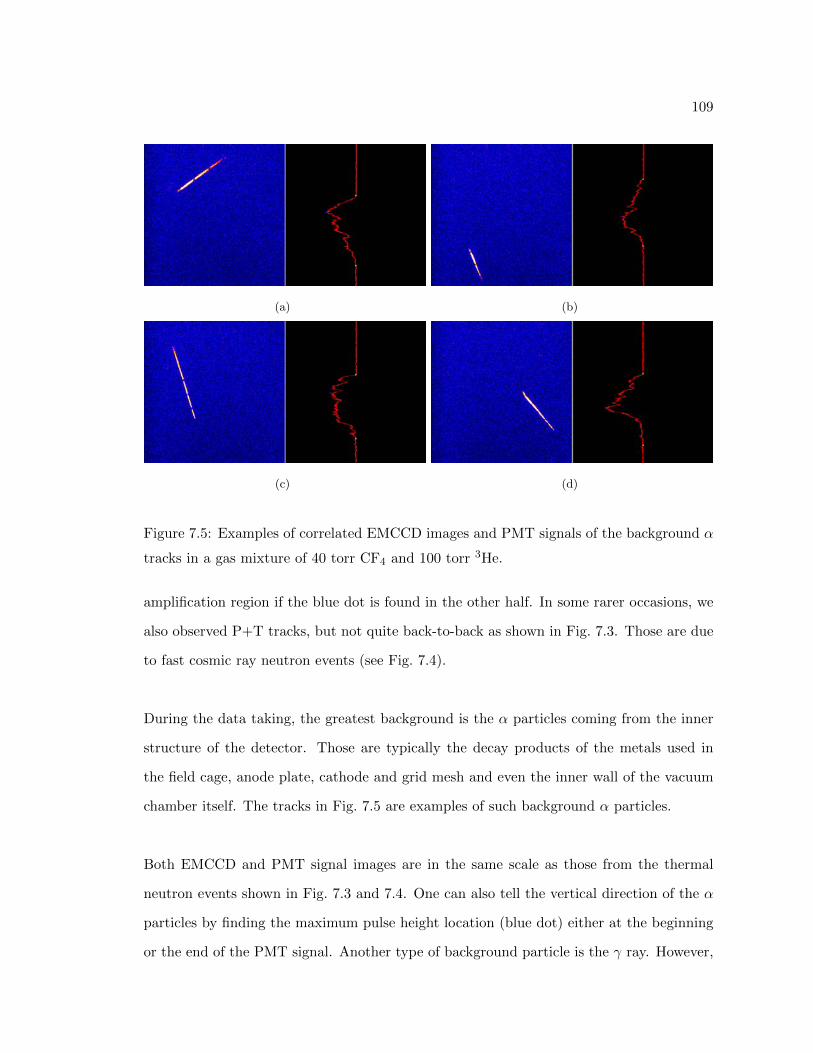
109
(a) (b)
(c) (d)
Figure 7.5: Examples of correlated EMCCD images and PMT signals of the background α
tracks in a gas mixture of 40 torr CF4 and 100 torr 3He.
amplification region if the blue dot is found in the other half. In some rarer occasions, we
also observed P+T tracks, but not quite back-to-back as shown in Fig. 7.3. Those are due
to fast cosmic ray neutron events (see Fig. 7.4).
During the data taking, the greatest background is the α particles coming from the inner
structure of the detector. Those are typically the decay products of the metals used in
the field cage, anode plate, cathode and grid mesh and even the inner wall of the vacuum
chamber itself. The tracks in Fig. 7.5 are examples of such background α particles.
Both EMCCD and PMT signal images are in the same scale as those from the thermal
neutron events shown in Fig. 7.3 and 7.4. One can also tell the vertical direction of the α
particles by finding the maximum pulse height location (blue dot) either at the beginning
or the end of the PMT signal. Another type of background particle is the γ ray. However,

110
the amount of energy a γ ray loses per unit length due to the interaction with the gas
molecules and atoms is typically lower than the PMT threshold, and the majority of them
are not even recognized. Even though some managed to trigger the system, the EMCCD
track finding program will not recognize it as a particle track because it is as low as the
background level and cannot be identified as a track. This means that our prototype Dark
Matter detector is essentially free of γ ray background, and all we have to be careful of is
the α particle background.
7.3 Thermal Neutron Data Result
The total live time of this 3He calibration experiment was 3,462 hours. Fig. 7.6 is the
scatter plot of the first day of data taking captured by an EMCCD camera. The x axis
is the two-dimensional projected track lengths of the particles onto the anode plane in
centimeters, and the y axis represents the amount of total light captured per track in the
typical counting unit of a CCD camera, ADU, or Analog to Digital Unit. Compared to
the previous runs without mixing 3He gas, it is obvious that there is a clump of partial
and full tracks from the thermal neutron events. As mentioned above, the energy given to
a proton and triton pair by such an event is always 764 keV, which in this scatter plot is
roughly equivalent to ∼75,000 ADU level.
In Fig. 7.6, the proton plus triton tracks that are fully contained within the region of the
detector lie horizontally in the ∼75,000 ADU region. Those with shorter projected length
indicate that they have a vertical component, which cannot be identified just by this scat-
ter plot. One can also find a fairly linear band of projected length vs. total ADU level.
This band of tracks is from those partially contained proton plus triton tracks in the anode
region of the detector. Those background α particles scatter around in the whole region.
In particular, those that are above the energy of 764 keV are extremely easy to distinguish.
The next scatter plot contains the same particle data information, but from the PMT data.

111
Figure 7.6: A scatter plot of 2D projected lengths vs. the energy deposited (in units of the
EMCCD’s ADU value) of particle tracks in the gas mixture of 40 torr CF4 and 100 torr
3He over one day of data taking.

112
Figure 7.7: A scatter plot of PMT pulse widths vs. the energy deposited (in units of the
PMT’s integrated pulse height ’V·s’) of particle tracks in the gas mixture of 40 torr CF4
and 100 torr 3He over one day of data taking.
The x axis here represents the signal width of the triggered particles in seconds, where the
y axis is the integrated pulse height in units of voltage multiplied by seconds.
An amazing match can be seen between the typical shape of the scatter plots provided by
the EMCCD and PMT. Both Fig. 7.6 and 7.7 offer the same information about the par-
ticle tracks, which are the range vs. energy but in different units measured with different
devices. The EMCCD measures the 2D projected length, where the PMT provides the
missing vertical length of the tracks. One can also see the linear relationship in energy
observed measured by the EMCCD and PMT.

113
Figure 7.8: The energy deposited measured by the PMT vs. EMCCD. This shows a good
linear relationship between data taken by the EMCCD and PMT.
The x and y axes in Fig. 7.8 are the energy of the particles obtained individually by the
PMT and EMCCD camera respectively. The typical energy resolution of this prototype
Dark Matter chamber is about 20 % for the σ value. The energy resolution varies over time
mainly due to the aging of the detector gas, which I will discuss later. Other reasons that
contribute to the deviation of the energy measurements are the disturbance of scintillation
due to the spacer material, parameters of choice that mark the border between the particle
track and background level in the EMCCD track recognition program, and parameters
chosen to determine the leading and trailing edges of the PMT signals.

114
7.4 Determining the 3D Full Track Length
By utilizing the pulse width data obtained by the PMT, I can extend the 2D projected
length of the particle tracks shown in Fig. 7.6 into a proper 3D length. However in order to
achieve this goal, a knowledge of the electron drift velocity under the given gas conditions
is essential. The value of the electron drift velocity for a gas mixture of 40 torr CF4 and
100 torr 3He cannot be found in any publication. The method I have chosen to take is to
find the best fit for the scatter plot of EMCCD projected length vs. PMT vertical length
pulse width. In a simple model, the vertical component of the particle tracks would be
obtained by multiplying the pulse width in seconds by the electron drift velocity. In my
attempt at doing so, I took the electron drift velocity as a variable and searched for the
minimum value of the spread (s) of the expected proper length under the assumption of
the Gaussian distribution. In a simple model,
proper length =√
(projected length)2 + (pulse width× vdrift)2
where vdrift is the anticipated electron drift velocity in units of cm/s. The advantage of
this approach is that the result is much less affected by the change in gas quality over time.
Fig. 7.9 is the result from such an attempt. By analyzing all appropriate correlated data
of the EMCCD and PMT information, I have come to the conclusion that the electron
drift velocity in such gas mixture is 3.5 cm/µs. Fig. 7.10 shows the corrected horizontal vs.
vertical particle tracks with the chosen electron drift velocity in this particular gas mixture.
Once I acquired the correct electron drift velocity for this gas mixture using the method
discussed above, I used the PMT data to correct the 2D projected length vs. energy de-
posited scatter plot seen in Fig. 7.6. Fig. 7.11 shows the modified version of Fig. 7.6 with
the estimated proper track lengths, and Fig. 7.12 presents the magnified image of the P+T
tracks distribution in the scatter plot (both partially- and fully-contained). Here, the x-axis

115
Figure 7.9: A polynomial fit was applied looking for the minimum σ fluctuation of the
proper length, having the drift velocity as a variable in the x-axis. The least σ means the
fluctuation of the proper length is at its minimum; thus, the clump of the 764 keV tracks
is the tightest.
is for the proper length of the particle tracks, while the y-axis is the energy of the particles
represented in ADU. One can see that the corresponding tracks of many data points that
had the vertical component have shifted to the right in the scatter plot, and it ended up
with a much denser clump for the 764 keV of proton plus triton tracks band for both fully
and partially contained. Fig. 7.13 shows the superposition of the expected range-vs.-energy
distributions of the ion/recoil tracks predicted by SRIM simulation on our corrected data.
Although the partially-contained P+T band would not perfectly align with a single proton
range vs. energy plot, Fig. 7.13 shows a good match of the data and simulation.
7.5 Change of Gas Gain and Energy Threshold
When the gas is placed into the vacuum prototype chamber, it ages over time and the
scintillation efficiency goes down. There are several factors that contribute to this aging
of the gas, but the residual impurity left inside the chamber and outgas from the material

116
Figure 7.10: A scatter plot of the projected vs. estimated vertical particle track lengths.
Once the electron drift velocity is properly chosen, the full 764 keV tracks should make a
quarter-circular shape with the full length of ∼10 cm.

117
Figure 7.11: The modified scatter plot with the estimated proper lengths vs. the energy
deposited (in units of the EMCCD’s ADU value) of particle tracks in the gas mixture of
40 torr CF4 and 100 torr 3He over one day of data taking.

118
Figure 7.12: The magnified version of the previous scatter plot (see Fig. 7.11) with the
estimated proper lengths vs. the energy deposited (in units of the EMCCD’s ADU value)
of particle tracks in the gas mixture of 40 torr CF4 and 100 torr 3He over one day of data
taking. The dense clump at the length ∼9 cm (or ∼60,000 ADU) are the fully-contained
P+T tracks. Points with shorter length (or smaller ADU values) are partially-contained
P+T tracks - some go out of view before stopping.

119
Figure 7.13: The modified scatter plot superimposed with the SRIM simulation of the
expected particle ranges of a proton, helium, carbon, and fluorine ions.

120
Figure 7.14: The change of gain over time measured by the EMCCD and PMT. We used
the 764 keV of P+T tracks energy as a calibration. There was no data acquisition on days,
such as 140, where the plot seems to be missing data. For clarity, error bars are not shown.
used are chiefly responsible for the degradation of the gas quality. In order to minimize the
chance of residual impurities, we specifically use high vacuum components, including the
vacuum chamber itself. When the experimental vacuum chamber is empty, the chamber
pumps down to a very high vacuum pressure on the order of 10−7 torr. However, once all
necessary components are introduced into the chamber, the minimum achievable pressure
goes up by at least factor of 100. This is due to the outgassing effect from all the material
inside. The only way to minimize the effect from outgas is to keep pumping out the cham-
ber as long as possible while simultaneously baking out the chamber and components at
the same time. The degradation of the gas lowers the scintillation efficiency of the particle
tracks. Fig. 7.14 shows the change of the scintillation gain over time for the above gas
mixture of 40 torr CF4 and 100 torr 3He.

121
The rate of gas degradation tends to slow down as time passes. During the first month of
data taking, the gain loss measured by the PMT is much steeper than that by the EM-
CCD camera. This is mainly due to the automated particle track finding program. The
background level does not change over time, while the actual particle track scintillation
degrades over time. Thus, in effect, the gain loss analyzed through the EMCCD data slows
down as shown in Fig. 7.14. On the other hand, the integrated pulse height measured
with the PMT has very little effective background compared to the case of the EMCCD;
thus, the PMT gas gain depends most strongly on gas quality. Another important fact
one can see in Fig. 7.14 is that at one point, the gradual decrease in gain of the EMCCD
data surpasses that of the PMT. This is caused by aging of the EMCCD chip. This aging
effect of the EMCCD chip is a well-documented phenomenon. When the photoelectrons
are multiplied in the Electron Multiplying register of the camera, some electrons get stuck
in the register potential well over long periods of use. This lowers the capability of the
EM gain of the camera, and causes the ADU level for each track data outcome to de-
crease. The rate of the EMCCD chip aging varies by the usage: duration, light level,
EM gain parameter, etc. In our data, I concluded that roughly 10 % of the gain loss in
the EMCCD data is due to the aging effect of the camera itself. The gain loss due to
the gas degradation also influences the energy threshold of the measurement. Fig. 7.15 il-
lustrates the change in the energy threshold measured by the EMCCD and PMT over time.
As mentioned above, the background subtraction in acquiring the integrated pulse height of
the PMT data is very minimal; thus, the change in gain measured is more directly related
to the actual change of the gas degradation. The parameter set for the EMCCD particle
track recognition program has a fixed value; therefore, it makes sense that the threshold
value of the particle recognition does not change over time. However, the actual value of
the light level measured would of course be lower as shown in Fig. 7.15 in the gain change
plot.

122
Figure 7.15: The energy threshold and its change over time of the prototype DM detector
used as a thermal neutron detector in the specific gas mixture setting of 40 torr CF4 and
100 torr 3He. Compared to the stable threshold level of the EMCCD program recognition,
the PMT threshold keeps increasing over time due to gas gain loss until it comes to a
saturation level.

123
Fig. 7.16 is the polar angle distribution of the direction of the proton plus triton ejections
from the thermal neutron capture events. 0 means that the interaction occurred com-
pletely horizontally and 90 indicates that it was vertical. The resolution of this polar
angle data is ±9. Due to the rigidity of how the track recognition program defines the
boundary of the particle track above the background level in the EMCCD image, and lead-
ing and trailing edges from the PMT signals, it is very difficult to define any particle as
perfectly horizontal or vertical. Also, I need to point out that some of the tracks used for
this analysis could have come from the elastic collisions of the 3He nuclei with neutrons;
however, a mere comparison of the cross sections indicates that the neutron absorption
events are at least 1,000 times more likely to occur than the elastic collisions, so this effect
should be very minimal. As also can be seen from the distribution of the thermal neutron
events in the projected vs. vertical track lengths plot (see Fig. 7.10), I anticipate that
we are missing some of the vertical tracks due to missing triggers. Under the assumption
that proton plus triton tracks from the thermal neutron capture events would travel in all
radial directions equally, I estimate that the data set is missing approximately 13.5 % of
the actual events due to the reason I cited before.
7.6 Thermal Neutron Flux
The origin of the thermal neutrons could be either cosmic ray oriented or Earth crust ori-
ented. Those that originate from cosmic rays reach the surface of the Earth, bumping onto
obstacles and slowing down, and end up as thermal neutrons. On the other hand, those
that come from the Earth’s crust are the typical result of heavy nuclear decay interactions.
It is also known that the background Rn rate has some seasonal and daily variations due
to the use of air conditioning or heating, and Rn is one of the heavy atoms that would
decay and emit α particles which can interact with light nuclei to produce neutrons.
When a thermal neutron enters the detector, the mean free path (M.F.P.) of the neutron

124
Figure 7.16: The polar angular distribution of the P+T tracks in the gas mixture of 40 torr
CF4 and 100 torr 3He.
is 1/(n·σ) cm, where n is the number density of the 3He, and σ is the capture cross section
of thermal neutron with 3He, which is 5333 barns (=5.333×10⁻²¹ cm2) for typical thermal
neutrons at room temperature. Assuming N for the neutron flux (in /s/cm2), and S for
the area of the detector (in cm2), the rate of neutrons entering the detector is N·S. The
reaction rate is N·S·H·n·σ, where H is the detector thickness (in cm). The thermal neutron
flux N is the unknown. Once the rate of capture events is known, this rate divided by
the sensitive volume equals to N·n·σ. For the prototype Dark Matter detector filled with
100 torr of 3He gas, this equals to N·1.87×10⁻². Fig. 7.17 is the thermal neutron detection
rate per volume over the data taking period. However, there are some periods of time that
data taking did not take place. As mentioned above, the gas degradation over time induces
the lowering of the energy threshold. In order to compensate for any resulting loss of trig-
gers, I have made a correction to the interaction rate for this change in the energy threshold.
The rate of the capture events is fairly uniform throughout the data taking period. There
seems to be a rate fluctuation at every 2 months. There has been a publication on the
lunar period influence on the thermal neutron rate by Alekseenko, et al. However, our data

125
Figure 7.17: The thermal neutron absorption rate and its change over time obtained in the
gas mixture of 40 torr CF4 and 100 torr 3He. The energy threshold correction has been
applied to the rate to compensate for the missing triggers due to the gas disintegration.
126
does not seem to match what Alekseenko, et al. concluded (Alekseenko et al., 2007, 2009).
The typical interaction rate of 8.5×10⁻⁶ /s/cm3 should be equal to the flux of thermal
neutrons multiplied by 1.87×10⁻² /cm. Finally, taking into account the missing tracks in
the triggering/analysis process that I mentioned earlier, the thermal neutron flux in the
4th floor of the PRB laboratory at Boston University is estimated as 5.3×10⁻⁴ /s/cm2.
The prototype Dark Matter detector has shown performance with an energy threshold as
low as 50 keV in a pure 40 torr CF4 gas and with a great sense of directionality. Al-
though we also learned how a gas degradation affects the energy threshold or data quality,
etc, we have not yet begun applying the gas circulation system, which will allow us to
maintain the gas quality for much longer periods of time. The use of the PMT minimized
the ambiguity of the direction of the particle tracks entering the detector. Particularly
for Dark Matter experiments with directionality, it is crucial that we tell the vertical com-
ponents from horizontal ones, in addition to the capability of telling the head-tail direction.

Chapter 8
Cylon: A New Direction-Sensitive Fast
Neutron Detector
8.1 Introduction to Cylon
After building a BU prototype Dark Matter detector with successful directionality read-
outs using both an EMCCD and PMT, we have come to appreciate this type of detector’s
application as a direction-sensitive fast neutron detecting device. On top of the scientific
application of such a device, this kind of detector could, in theory, be utilized as a secu-
rity device which identifies fast fissile neutrons emitted by heavy nuclear materials such as
plutonium. This application is the primary motivation behind constructing a new detector
that both uses and improves upon the knowledge we already acquired by from building a
prototype direction-sensitive time projection chamber. We have named the new nuclear
recoil detector in this project ’Cylon’, a new generation of direction-sensitive neutron de-
tectors (see Fig. 8.1).
There are several new design criteria for such a neutron detector. First, it is necessary to
increase the detector’s sensitivity in detecting nuclear recoils induced by fast neutrons from
fissile materials. In order to do so, we either increase the sensitive volume of the detector
or increase the detector’s gas pressure inside the chamber. The Cylon detector should be
portable so that we can easily put the detector into an actual working field outside of a
127

128
(a) (b)
Figure 8.1: (a) The cross sectional sketch (Wellenstein and Dushkin), and (b) the actual
Cylon neutron detector.

129
scientific lab. Furthermore, the use of 4He gas is an advantage for this detector because of
the large neutron cross section with 4He at fission neutron energy region. The use of 4He
gas is not necessarily new to us; as I explained earlier, we already have a good amount of
experience with such a gas mixture through our prototype Dark Matter detector experi-
ments. In order for the equipped EMCCD and PMT to be able to read out the optical
signal, mixing in some ratio of CF4 gas is also essential in order to achieve the necessary
amount of scintillation. Finally, another criterion for building such a detector is the neces-
sity of a fast triggering system and an effective method of correlating the data from both
the EMCCD and PMT signals. This is essential to get a full understanding of the particle
tracks.
The basic components that constitute this new detector are the same as those of the pro-
totype Dark Matter detector. We are planning to use the same EMCCD camera because
of its superior signal readout ability. However, one big change made to the optical readout
system is the change of the lens. Prior to this, we have used a Schneider Xenon 0.95/17
lens to go with the EMCCD camera, due to its large angle view. Although the lens was well
matched to the task, one drawback of the lens was the drop off in light collection efficiency
toward the edges. Another downside of this lens is its small surface area, which is only
about 36 mm in diameter. To improve the design, we have had Schneider custom-make a
new Cylon lens (see Fig. 8.2). The diameter of this new lens has been improved to 60 mm.
Having set and designed the distance between the lens surface and the amplification region
to about 36 cm, this change in the surface area of the lens will result in a 180 % increase
in the efficiency of the light collection.
One attempted improvement to this new Cylon custom lens is the uniformity of the light
collection throughout the lens surface. Fig. 8.3 shows the amount of light collected divided
by the equivalent PMT signals’ integrated pulse height as a function of the location of the
Bragg peak in radius from the center of the lens. An 241Am α source was used for this

130
(a) (b)
Figure 8.2: (a) The cross sectional sketch (Wellenstein and Dushkin), and (b) the ac-
tual custom-made Schneider lens made for the Cylon detector and attached to the Andor
EMCCD camera.

131
Figure 8.3: The drop-off ratio of the light collection on the new custom made Schneider
lens for Cylon. The drop-off effect is only within 10 % compared to the central region of
the lens, which is a tremendous improvement.
data, and the α emission was only single directional. Compared to the Schneider 17 mm
lens that we have been using for the prototype detector, the light collection efficiency of
the new lens is more spatially uniform and linear to the direction of the α particle tracks’
emission, and there is only about a 10 % loss at the edges of the custom-made Schneider
lens for Cylon.
Also for the Cylon detector, we have utilized a set of new PMTs, XP2017B from Photonis
(see Fig. 8.4(a)). This also increased our sensitive area for collecting scintillation light.
Compared to the old Hamamatsu R7400U-20 phototubes system, where a total of five
were used in the prototype Dark Matter detector, the use of four new Photonis phototubes
increases the light collection efficiency by roughly a factor of 10. We are also pleased that
by the Photonis PMTs’ superior sensitivity at the red end of the spectrum compared to
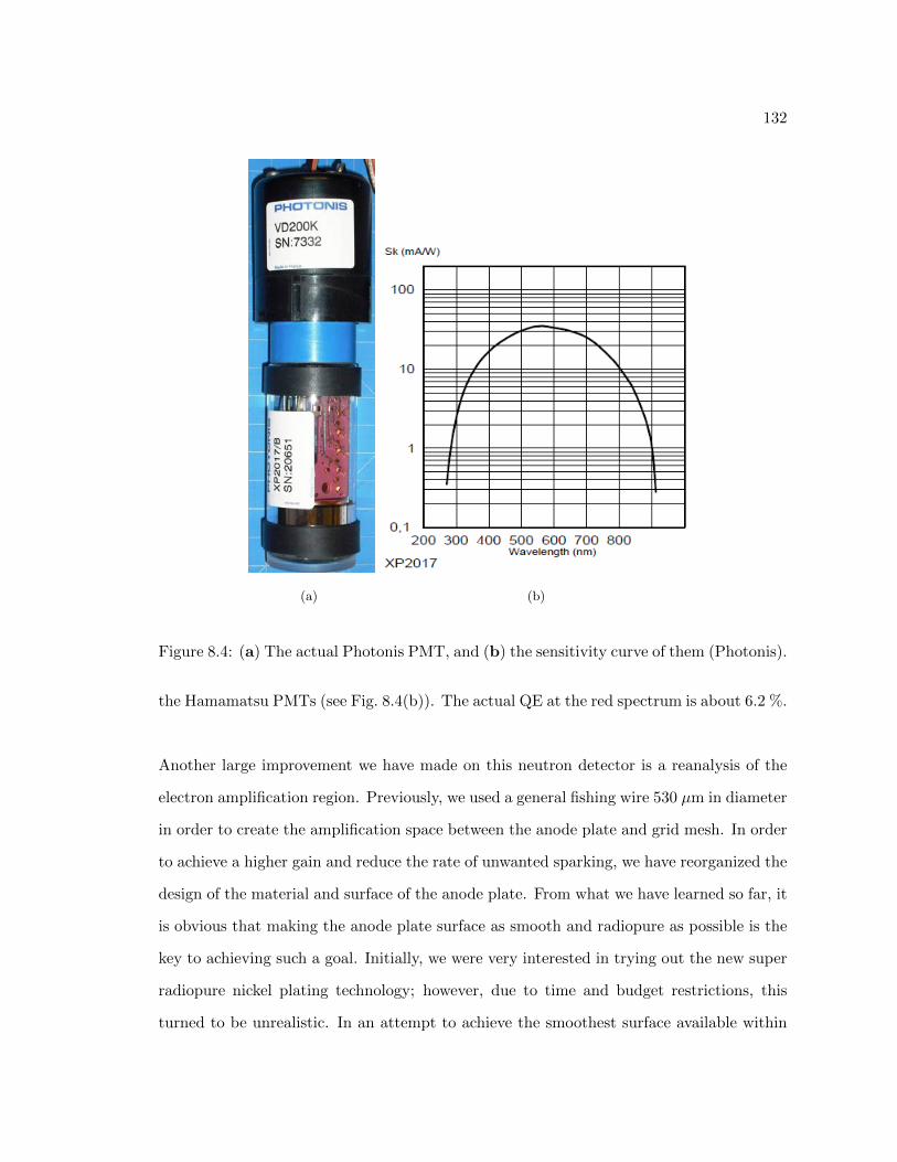
132
(a) (b)
Figure 8.4: (a) The actual Photonis PMT, and (b) the sensitivity curve of them (Photonis).
the Hamamatsu PMTs (see Fig. 8.4(b)). The actual QE at the red spectrum is about 6.2 %.
Another large improvement we have made on this neutron detector is a reanalysis of the
electron amplification region. Previously, we used a general fishing wire 530 µm in diameter
in order to create the amplification space between the anode plate and grid mesh. In order
to achieve a higher gain and reduce the rate of unwanted sparking, we have reorganized the
design of the material and surface of the anode plate. From what we have learned so far, it
is obvious that making the anode plate surface as smooth and radiopure as possible is the
key to achieving such a goal. Initially, we were very interested in trying out the new super
radiopure nickel plating technology; however, due to time and budget restrictions, this
turned to be unrealistic. In an attempt to achieve the smoothest surface available within

133
Figure 8.5: The custom-made mirror-finished copper anode plate seen underneath the
copper grid mesh separated with the 360 µm diameter optical fibers as spacers.
our budget, we looked into a mirror finish option for the surface of the anode plate. This
amazing surface mirror polishing job was done at Marena Industries, Inc. in Connecticut.
Fig. 8.5 presents the new amplification region of the Cylon detector. The surface of the
copper anode plate with a 30 cm diameter was mirror-finished so that the height variations
on its surface are less than a couple micrometers. The next improvement made to the
electron amplification region was the choice of the spacer material and diameter. Deciding
on the new spacer material actually required a lot of exploration and discovery. The mate-
rial had to be somewhat flexible so that, when voltage was applied, the mesh could ’push
down’ the spacer and keep the precise distance between the anode and grid. After some

134
study of the spacer material, we came to realize the importance of the spacer’s material
and structure. When placed in between the high voltage anode plate and grounded grid
mesh, the spacers work as a typical dielectric medium. When the material’s dielectric con-
stant is high, it gathers unnecessary amounts of charge where it touches either the anode
or grid. This causes an increase in the spark rate, or decrease of the applied voltage before
stable operation collapses. Therefore, we came to the conclusion that as long as the chosen
spacer material is strong and clean enough to maintain the integrity of the necessary space
between the anode and grid, a hollow-shaped tube is most ideal for such an application.
What we actually ended up using as the spacer for the Cylon neutron detector is an optical
fiber, Polymicro TSP250350. This is a general capillary fiber made of a fused silica hollow
tube with an inner diameter of ∼250 µm, wrapped with polyimide coating material and
an outer diameter of ∼360 µm. Thus, the actual spacing of the amplification region would
be 360 µm, which is an improvement from the previous 530 µm of space achieved with
the fishing wire. Because of the smoothness of the mirror-finished anode plate and low-
ered dielectric constant value of the spacer material for reduced local electric field where
it touches the anode or grid, we can still apply the same amount of voltage onto the anode
plate in the same gas configuration without inducing electric discharge despite the fact
that the space between the anode and grid has been decreased. This should give at least
50 % more gain in this region. On top that, the spark rate has been reduced to the order
of 1×10⁻⁴ Hz, which improves upon that of the prototype Dark Matter detector by at
least a factor of 10. This is due to the improved cleanliness inside the chamber in terms
of unnecessary outgassing and, in fact, means that the Cylon amplification region would
cause sparking events at a rate of only once or twice per hour while in standard running
mode.
The smoothness of the anode plate surface also contributes to increasing the energy res-
olution. Fig. 8.6 is from the 241Am α particle source, which was previously used in the
calibration of the prototype Dark Matter detector, placed at 3 cm from the amplification

135
Figure 8.6: The SRIM simulation and actual data of the 241Am α particles ranges in the
Cylon gas mixture of 40 torr CF4 and 600 torr 4He. Although the x-axis is the projected
track length, those α particles are emitted horizontally through a collimator and would not
make a huge difference to the real proper length.
region. The black dots are from the SRIM simulation. In the gas mixture of 40 torr CF4
and 600 torr 4He, typical α particles from this source have a range of around 10 cm. In
this region of an α emission, the energy resolution measured with this detector is as low as
4 % in σ. This is a noticeable improvement when compared to the previously-used Dark
Matter prototype detector’s typical energy resolution of 20 %. Fig. 8.7 also shows the
linearity between the EMCCD and PMT signals for the α particle tracks from the same
241Am source.
The field cage of the Cylon detector has also been increased to 25 cm (see Fig. 8.8). To-
gether with the whole 30 cm diameter of the anode plate, the sensitive volume of the Cylon
detector has gone up to ∼18 liters, which is roughly a 40 % increase compared to that of the
BU prototype Dark Matter detector. The material used inside the detector has also been

136
Figure 8.7: A scatter plot of the α particle tracks energy captured by the PMT vs. EMCCD.
This shows a very good linear relationship between signals from the two devices.

137
very carefully considered. All the necessary plastic components are made with an aerospace
engineering-grade material called Vespel SP1, which is known for its low outgassing quality.
It is also know as a sturdy material, so we can use it as posts to support all the field cage
rings and the amplification region. In our previous experience with the prototype detector,
we discovered that plastics, which contain copious amount of hydrogen, can cause some
charge-one particle backgrounds and that the resistors which separate the voltages on the
field cage rings are horrible α particle emitters. In Cylon, we have designed hollow Vespel
tubes that the resistors can be fitted into, so that any unfortunate α particles emitted from
the resistors will be stopped by the Vespel sleeves and cause no visible background in the
view of the EMCCD camera.
While we have kept the anode voltage at 620 v, the cathode voltage is now set to 2000 v.
This provides only 80 v/cm of drift electric field. In the typical gas pressure of our usage
of the TPC detectors, the higher the drift electric field, the smaller the electron diffusion.
So, our initial goal was to keep the same amount of electric field as that of the prototype
chamber (125 v/cm). However, due to the design, we could only apply 80 v/cm of electric
field. Fig. 8.9 is the transverse electron diffusion of α particle tracks placed at distance
of 3 cm from the amplification region in the above gas mixture. The σ squared value for
the Gaussian fit is about 1.39 mm2, and it is roughly a factor of two worse than what I
measured for the prototype detector with 125 v/cm of electric field applied in the same
gas configuration. This means the actual electron diffusion effect could get up to 50 %
worse compared to what we observed in the prototype Dark Matter detector. The second
plot shows the discrepancy between the electron diffusion values when two different drift
electric field values are applied. This increase of the electron diffusion will unfortunately
affect the EMCCD light level readings above the background level in our track recognition
program.
In the voltage settings stated above, we have used two types of gas mixtures; one is the

138
Figure 8.8: The 25 cm field cage rings made out of a pure copper for the Cylon detector.
The bottom side of the lid is also covered with the same copper plate to reduce the α
background from the SS304 lid. All the Cylon systems are supported by the rods made of
the Vespel SP-1 also as shown in the picture.

139
(a) (b)
Figure 8.9: (a) A Gaussian fit applied onto the transverse electron diffusion of the α
particle tracks in the Cylon gas mixture of 40 torr CF4 and 600 torr 4He, and (b) the
electron diffusion result (red marker) compared to that with a higher drift electric field
(black).
mixture of 40 torr CF4 and 600 torr 4He gas, which is targeted mainly for fast neutron
detection, and the other is adding another 50 torr 3He on top of the first gas mixture. The
second gas configuration is once again for the calibration of the new Cylon detector with
a sufficient number of naturally occurring thermal neutrons in the laboratory. Now that
the drift electric field is less than that of the previous prototype chamber, it is important
to understand the change in electron velocity, so I started analyzing the data with the 3He
gas mixture case.

140
8.2 Thermal Neutron Capture Event Data with Cylon De-
tector
8.2.1 Electron Drift Velocity
The Cylon detector was filled with a gas mixture of 40 torr CF4, 600 torr 4He and 50 torr
of 3He, and continuously took data for a total of 21 real days. Though some configurations
were modified during this data-taking period, I will only use the 17-day data set with all
the parameters fixed for the analysis here. The anode voltage was kept at 620 v, and the
cathode voltage was at 2000 v as mentioned above, which gives 80 v/cm of drift electric
field. In order to determine the electron drift velocity in this gas mixture, I employed the
same method that I used previously with the prototype Dark Matter detector. Fig. 8.10
illustrates an example of the distribution of data points in the projected horizontal vs.
vertical lengths graph. The total range of the proton plus triton from the thermal neutron
capture events in this gas content predicted by the SRIM simulation is roughly 5 cm.
Using the same technique I used previously and focusing only on the fully contained proton
plus triton track length of around 5 cm, and varying the electron drift velocity value to
achieve the tightest σ in the fit, I have determined the value of 0.865 cm/µm as the best
fit (see Fig. 8.11). Using this parameter, I can now create a scatter plot of the particle
tracks with their true 3D proper lengths. Fig. 8.12 shows the result over a one day run.
The x axis is the corrected particle track’s proper length using the electron drift velocity
obtained in the above process. In a rough comparison to the previously obtained data
from the prototype detector, the gain has increased by 75 % or more; however, the energy
resolution has worsened. Without any corrections, the estimated energy resolution for the
full length 764 keV proton plus triton tracks presented in Fig. 8.12 is about 30 %. This
is worse than that of the prototype chamber even considering the fact that the field cage
height has been increased by 25 % and the electric field applied in the electron drift region
has been lowered to 80 v/cm in order to avoid the spark events. When I analyzed a similar

141
Figure 8.10: A scatter plot of the projected vs. estimated vertical particle tracks lengths
in the gas mixture of 40 torr CF4, 600 torr 4He, and 50 torr of 3He. Once the electron drift
velocity is properly chosen, the full 764 keV tracks should make a quarter-circular shape
with the full length of ∼5 cm.
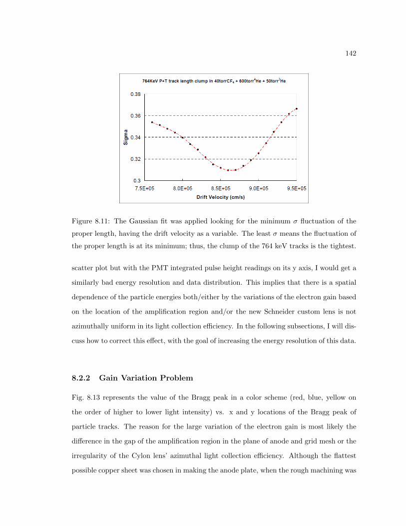
142
Figure 8.11: The Gaussian fit was applied looking for the minimum σ fluctuation of the
proper length, having the drift velocity as a variable. The least σ means the fluctuation of
the proper length is at its minimum; thus, the clump of the 764 keV tracks is the tightest.
scatter plot but with the PMT integrated pulse height readings on its y axis, I would get a
similarly bad energy resolution and data distribution. This implies that there is a spatial
dependence of the particle energies both/either by the variations of the electron gain based
on the location of the amplification region and/or the new Schneider custom lens is not
azimuthally uniform in its light collection efficiency. In the following subsections, I will dis-
cuss how to correct this effect, with the goal of increasing the energy resolution of this data.
8.2.2 Gain Variation Problem
Fig. 8.13 represents the value of the Bragg peak in a color scheme (red, blue, yellow on
the order of higher to lower light intensity) vs. x and y locations of the Bragg peak of
particle tracks. The reason for the large variation of the electron gain is most likely the
difference in the gap of the amplification region in the plane of anode and grid mesh or the
irregularity of the Cylon lens’ azimuthal light collection efficiency. Although the flattest
possible copper sheet was chosen in making the anode plate, when the rough machining was

143
Figure 8.12: The modified scatter plot with the estimated proper lengths vs. the energy
deposited (in units of the EMCCD’s ADU value) of particle tracks in the Cylon gas mixture
of 40 torr CF4, 600 torr 4He, and 50 torr 3He over one day of data taking.

144
Figure 8.13: The distribution of the energy gain for fully-contained P+T tracks of 764 keV.
A decreasing light intensity is color-coded from red-blue-yellow respectively.

145
done, the deviation from flatness was as large as 81000” because the original copper sheet
had not been tamper released. This is about 200 µm of space difference in the attempt
of making an amplification region of 360 µm. Though the polishing machinists did the
best they could, even more unexpected warping of the plate could have occurred when it
was sent to its final destination for mirror finishing. This was unavoidable due to copper’s
high conductivity to heat when grinding. Another factor that makes it difficult to keep the
amplification gap uniform is the way it is installed. The anode disk is held at 4 points, each
at 90 on its edge. The stretched copper mesh is set above the anode disk by sandwiching
the optical fibers mentioned above as the spacer. When the disk is bent (no matter how
small the deflection is) and held only at 4 locations, it is not easy to keep the separation
between the anode plate and grid mesh at all locations. On top of that, it is necessary
to keep the mechanical tension on the spacer caused by the anode disk pressing on it as
minimal as possible while simultaneously ensuring that the disk and mesh are separated
by a distance as close to the diameter of the spacer material as possible. For the same
reason mentioned above, it is not easy to achieve such a goal when the disk is held at only
4 locations. Considering those two points, it is reasonable that the variation of the gain is
in the shape very similar to the profile of deflection of the anode plate. When voltage is
applied across the amplification region, the electrostatic force pulls the mesh towards the
anode. Thus, any minor imperfection in the spacing would be resolved by the help of this
electrostatic force when running. However, there are certain parts of the anode plate edge
where the optical fiber is forced to bend and the electrostatic force is not high enough to
resolve it; thus, the gap between the anode and grid mesh gets greater than in other areas.
Hence the gain we observe in the central region of the view is the true gain that we would
find when 620 v is applied to a gap of 360 µm with the given gas mixture content. This
is very important information for any future design, especially if the amplification region
gap is as small as or even smaller than what it is now. For the Cylon detector, it is not
easy to rebuild/redesign the amplification region, and so this gain fluctuation by location
needs to be resolved by data correction.

146
8.2.3 Applying Data Correction to Improve the Gain Non-Uniformity
In order to make this correction for the gain non-uniformity, we used the data of the 3He
mixture run because the 764 keV emitted by all thermal neutron capture events serves as
an excellent calibration source. We mapped out the gain variation obtained (see Fig. 8.13)
for the fully-contained P+T track sets bin by bin, determining the average value in each
local bin area, and normalized it to make a smooth correction factor. Fig. 8.14 is the newly
corrected scatter plot of particle tracks’ full length vs. energy measured with EMCCD from
the 3He mixture run. The energy resolution is approximately 20 %, which is mainly due
to the distribution of the electron drift length. Due to the smearing effect of the particle
tracks’ width, the deposited energy recognized by the track finding program decreases as
the electron drift length increases.
As I have shown so far, achieving a great energy resolution with the EMCCD information
is very difficult due to the electron diffusion effect. In order to avoid this effect on the
energy resolution, the particle energy should be measured with large-sensitive-area PMTs
in our future detector. Although Cylon is equipped with four PMTs with larger total
surface area than that of the BU prototype detector, we could not fully achieve this goal,
primarily due to the spatial dependence of the particle energies that I discussed in the
previous subsections.
8.2.4 Change of Triggering System
Another one of the positive changes made for the Cylon fast neutron detector is its trig-
gering system. Previously with the prototype detector, we had assigned one PMT as a
designated triggering device using a preamplifier and amplifier. As the total surface area
of the PMT of the Cylon is much greater than that of the prototype detector, we now

147
Figure 8.14: A correction factor has been applied to the data presented in Fig. 8.12 in order
to minimize the spatial dependence of the particle energies. The fully contained P+T tracks
due to the thermal neutrons absorption of 3He clump much tighter near ∼4.7 cm in the
scatter plot.

148
trigger the system directly through those PMTs while we simultaneously acquire the sig-
nal. Discarding a preamplifier and amplifier and the use of NIM devices minimizes the
signal delay and also the probability of acquiring a mismatched pair of data files from the
EMCCD and PMT. Taking all the time required to read/write data for both readouts into
consideration, we assigned 2 seconds of dead time after each triggering by signals so that
no new trigger would occur before the computers were ready to record new sets of data.
This new triggering system eliminates a large amount of miscorrelation within the data
files. As stated above, when we used the time stamps of the file created as a source of
correlation, the average recovery efficiency was only up to 70 %. With the new triggering
we use with Cylon, a typical failure rate for the file correlation is on the order of 0.1 %,
which means the recovery efficiency goes up to 99.9 %.
Although this Cylon triggering system is more refined when it comes to the efficiency of
data correlation, it is missing out the triggers for a majority of the vertical types of particle
tracks. In the previous triggering system with the preamplifier and amplifier, the signal
from each track was integrated before triggering; thus, there was no difference in trigger-
ing on horizontal and vertical particle tracks. However, when one triggers directly on the
PMT signal, the individual pulse height along the track goes below threshold for some of
those vertically moving particle tracks. Fig. 8.15 shows the different PMT pulse shapes of
horizontally and more vertically moving α particle tracks respectively.
Because the electron drift velocity in this gas mixture is much smaller than that of the
ion motion in gas, horizontally moving tracks leave a tall and sharp pulse, which has no
problem triggering the system. As before, the green dot indicates the leading edge and
the yellow dot points to the trailing edge of the PMT pulse. On the other hand, when
the particle moves more vertically, because of the slow drift velocity, the scintillation is
distributed over a much longer period of time, and each pulse height per unit time gets
very low. To ensure it is above the background level, the triggering level is kept at 30 mV.

149
(a) (b)
Figure 8.15: The correlated EMCCD images and PMT signals of the background α particle
in the Cylon gas mixture of 40 torr CF4, 600 torr 4He, and 50 torr 3He. The α particle
is moving more (a) horizontally and (b) vertically. It may be impossible to resolve the
differences with EMCCD images alone; however, the PMT signals are clearly different
in the pulse width. This is because the electron drift velocity is very small in the high
concentration of 4He gas.
The voltage applied to the PMT for this run was 1.4 kV. If it is higher, the trigger begins
catching the background γ ray level, but if lower, it would not trigger as many of the verti-
cally moving particles. Fig. 8.16 shows the distribution of polar angles of the P+T tracks
recorded by this Cylon detector. The resolution of the polar angle data shown in Fig. 8.16
is ±4. Compared to the distribution of polar angles of tracks in the prototype detector
shown earlier (see Fig. 7.16), one can see that it is missing a majority of the vertical track
triggering events. In a similar estimation done for the prototype Dark Matter detector’s
case, my approximation of the missing fraction of triggers goes up to 37.6 % of the whole
P+T events in this run.
8.2.5 Thermal Neutron Flux by Cylon
In order to identify the energy threshold of the Cylon detector with naturally occurring
thermal neutron capture events, I focused only on those events that occurred within the
central 10 cm radius region of the anode plane, where the electron gain is fairly uniform be-

150
Figure 8.16: The polar angular distribution of the P+T tracks in the Cylon gas mixture
of 40 torr CF4, 600 torr 4He, and 50 torr 3He.
cause of the uniform amplification gap. The following energy threshold plot (see Fig. 8.17)
is for the correlated data sets, which means that the actual threshold for the PMT trig-
gering would be even lower; however, I am only interested in those correlated files that
were categorized as ’with feature’ by the EMCCD track analysis program. Thus in a strict
sense, this plot is equivalent to the previously shown EMCCD ’recognition’ threshold of the
prototype Dark Matter detector. Compared to the prototype detector’s energy threshold
for the thermal neutron capture events, there is an improvement by a rough factor of two.
Fig. 8.18 shows the fluctuation of the rate of the thermal neutron capture events triggered
and recognized by the particle track recognition program. Although we could only run
the Cylon detector with the 3He gas mixture for a shorter period of time due to our data-
taking schedule, what we have obtained is good enough to give us a good idea about the
interaction rate. Fig. 8.19 shows the thermal neutron capture events by both prototype
detector and this new Cylon detector superimposed in the same unit of neutron absorption

151
Figure 8.17: The energy threshold of the Cylon detector with the gas mixture of 40 torr
CF4, 600 torr 4He, and 50 torr 3He.
rate per unit volume per unit pressure of 3He and/or 4He gas after the missing trigger
correction by polar angles. Thus, as one can see in this plot, under the same conditions,
both the prototype Dark Matter and the Cylon detectors observed the thermal neutron
capture events with a high amount of consistency. This supports my previous conclusion
of the value 5.3×10⁻⁴ /s/cm2 for the thermal neutron flux.
8.3 Cosmic Ray Neutron Data with Cylon as a Fast Neutron
Detector
8.3.1 Initial Motivation of Cylon Fast Neutron Detector
The primary purpose of the Cylon detector is its use for fissile neutron detection with
great sense of directionality. With the capability our detector can offer, it is plausible to
make a fissile neutron sensitive detector that can locate the origin of heavy nuclei such

152
Figure 8.18: The thermal neutron capture event rate with the Cylon detector using the
gas mixture of 40 torr CF4, 600 torr 4He, and 50 torr 3He over two weeks. The energy
threshold correction has been applied to the rate to compensate for the missing triggers
caused by the disintegration of the gas.

153
Figure 8.19: The comparison of the thermal neutron capture event rates, measured with
the BU prototype Dark Matter detector in blue (100 torr of 3He used) and the new Cylon
fast neutron detector in red (50 torr of 3He used).

154
as plutonium or uranium with great precision, based on the incoming neutrons’ direction
and energy. A plutonium neutron spectrum peaks at around 1 MeV, just like that of 252Cf
shown earlier. In this energy region, the neutron cross section with 4He atom also peaks up
to 7 barns. When the Cylon detector is filled up to 5 bar of mixed gas pressure of the ratio
CF4:4He=1:15, the neutron detection efficiency of 4He gas goes as high as 1.8 %. Such a
detector could identify more than 1 fissile neutron recoil per second from a 4kg weapon’s
grade plutonium located 20 m away from the detector (Ahlen, 2009). By expanding the
detector size up to 1 m3, the detection rate goes as high as ∼10 per second. Another sig-
nificant usage on such a detector is to identify delayed neutrons from 235U. Unlike prompt
neutrons that are emitted as a result of a nuclear fission, delayed neutrons are emitted
in a fraction to tens of seconds after the prompt neutrons emission in a process of beta
decay. The typical half lives of those delayed neutrons from 235U are well known. By
shooting such a uranium source with fast neutrons, we can induce those delayed neutrons,
a technique which is called an ’active interrogation.’ I will discuss this technique at the
end of the section.
The initial intention of the Cylon fast neutron detector is to run it with the gas mixture of
CF4 and 4He. Although it is nice to have some 3He gas mixed in, the scarcity of 3He gas
is becoming serious, and our objective was to construct an effective fast neutron detector
without using 3He gas. In the standard running mode of Cylon, we exploit the gas mixture
of 40 torr CF4 and 600 torr 4He. As stated earlier, the anode voltage is kept at 620 v, and
the cathode voltage is at -2000 v, which gives 80 v/cm of the drift electric field. The images
in Fig. 8.20 are examples of the cosmic-ray-neutron-induced nuclear recoils captured by the
Cylon detector.

155
(a) (b)
(c) (d)
Figure 8.20: The correlated EMCCD images and PMT signals of the cosmic-ray-neutron-
induced recoils in the Cylon gas mixture of 40 torr CF4 and 600 torr 4He.
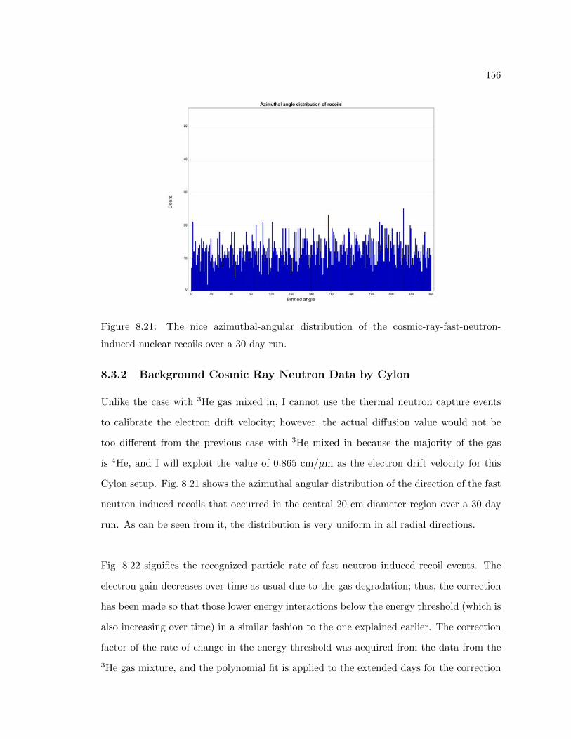
156
Figure 8.21: The nice azimuthal-angular distribution of the cosmic-ray-fast-neutron-
induced nuclear recoils over a 30 day run.
8.3.2 Background Cosmic Ray Neutron Data by Cylon
Unlike the case with 3He gas mixed in, I cannot use the thermal neutron capture events
to calibrate the electron drift velocity; however, the actual diffusion value would not be
too different from the previous case with 3He mixed in because the majority of the gas
is 4He, and I will exploit the value of 0.865 cm/µm as the electron drift velocity for this
Cylon setup. Fig. 8.21 shows the azimuthal angular distribution of the direction of the fast
neutron induced recoils that occurred in the central 20 cm diameter region over a 30 day
run. As can be seen from it, the distribution is very uniform in all radial directions.
Fig. 8.22 signifies the recognized particle rate of fast neutron induced recoil events. The
electron gain decreases over time as usual due to the gas degradation; thus, the correction
has been made so that those lower energy interactions below the energy threshold (which is
also increasing over time) in a similar fashion to the one explained earlier. The correction
factor of the rate of change in the energy threshold was acquired from the data from the
3He gas mixture, and the polynomial fit is applied to the extended days for the correction

157
Figure 8.22: The cosmic ray neutron capture event rate with the Cylon detector of the gas
mixture of 40 torr CF4 and 600 torr 4He over 30 days of data taking. The energy threshold
correction has been applied to the rate accordingly to compensate for the missing triggers
due to the gas disintegration.
factor for the energy threshold.
Shown in Fig. 8.23 is the corrected particle track lengths vs. the energy deposited, with
the superposition of both a SRIM simulation result and the actual data from the Cylon
detector filled with mixed gas of 40 torr CF4 and 600 torr 4He. It focuses on the typical
nuclear recoil energy region. As previously mentioned in Sec. 8.2.3, the correction to the
spatial dependence of particle energies is applied, and the outcome energy resolution is
approximately 20 %. Based on the fit analysis from the SRIM simulation as shown in
Fig. 8.23, I have concluded that 0.3 % is protons, 0.9 % is muons, 92.4 % is helium nuclei,

158
Figure 8.23: An overnight Cylon scatter plot data fit to the SRIM simulation. This presents
a low∼medium energy region to focus on the cosmic-ray-neutron-induced helium nuclear
recoils.
and the remaining 6.4 % comes from either carbon or fluorine recoils. With the given
energy resolution, it is not plausible to effectively separate carbon and fluorine recoils.
Taking the neutron energy of ∼1 MeV where the cross section of helium nuclei becomes
as large as ∼7 barns, the average neutron interaction rate with our detector of 2.7×10⁻⁷
/s/cm3 puts forward to the cosmic ray neutron flux of ∼1.7×10⁻³ /s/cm2. As mentioned
earlier, the typical neutron flux at sea level is on the order of 1×10⁶ /day/m2, which is
roughly on the order of 1×10⁻³ /s/cm2. Our result with the Cylon detector is consistent
with this value. Given the directionality capability and sensitivity of as low as the order
of 100 keV, Cylon performs very well as a fast neutron detector.

159
8.4 Detector Improvements
There are a few other improvements being developed for both Cylon and the DMTPC Dark
Matter detector. For Cylon in particular, two important and necessary improvements are
the increased sensitivity and pulsed timing of the high voltage supply on the anode plane
and EMCCD and PMT triggering. Also for both Cylon and the Dark Matter detector,
maintaining the quality of the target gas in the detector is a very important issue for keep-
ing the signal gain stable.
8.4.1 Improvement for Active Interrogation
As I briefly explained earlier, the first criterion of a sensitive neutron detector would be
achieved by increasing the detector pressure through a modification of its structural design,
and the other by using a fast rise/fall time high voltage supply and some NIM devices. The
delayed neutron recognition with such a direction-sensitive neutron detecting device would
be very unique and useful in securing shipped items in cargo without actually opening
them and preventing nuclear terrorism. We can pulse and synchronize the power supply
of Cylon detector with a fast neutron generator source so that Cylon’s power is turned off
during the irradiation of fast neutrons on uranium. Once the neutron generator is turned
off, Cylon is turned back on to detect any delayed neutrons in a pulsing mode. By making
this timing on the order of microseconds or less, our detector should be able to detect only
the featured delayed neutrons from such a material as uranium.
We have recently modified the triggering system capability of the Cylon neutron detector
with a pulsing functionality for both the amplification voltage and EMCCD and PMT
triggering timings. This new triggering system may be critical in the search for delayed
neutrons from uranium sources. The schematics shown in Fig. 8.24 explain how it works.
Once the Cylon receives a signal from the neutron generator turning on, we can set the
delay before Cylon turns on its anode high-voltage in order to avoid the sparking events,

160
Figure 8.24: The schematics of the timings of turning on the anode high-voltage and
triggering the EMCCD and PMT after the incoming signals from the sources such as
neutron generators with the pulse frequency of ’f’ Hz.
which are caused by fast neutrons from the generator. After some delayed time, the neu-
tron generator is turned off, and the Cylon anode turns on. In order to avoid the inevitable
voltage overshoot and RF noise, we also delay the triggering of the EMCCD and PMT.
Thus, while the EMCCD and PMT are active, the only source for the nuclear recoil in
the detector would be the delayed neutrons (assuming cosmic ray neutrons are rejected
later on). Both the EMCCD and PMT would be deactivated before turning off the anode
voltage for a clean procedure. Then the same cycle repeats. Upon a positive verification of
such a detection capability, we are planning to upgrade the detector to 1 m3 in size. With
a detector of this size, the sensitivity increases up to 8 % or more. It will be capable of
detecting - in a matter of seconds and with a great sense of incident direction - any fissile
nuclear material within 20 m.

161
8.4.2 Improvement for Gas Gain
For both the prototype Dark Matter detector and Cylon neutron detector, we chose to use
vacuum chambers. This is so we can pump out the air inside down to high vacuum level
and keep the gas quality as high as possible once the target gas is introduced. However,
as I have shown in the thesis, anything we introduce into the detector causes outgassing.
Outgassing contributes to the impurity of the gas inside and will, over time, cause a re-
duced signal level. Using low outgassing material is one way to minimize this problem;
however, more active method of cleaning the target gas becomes necessary in order to
carry on a long-run detector exposure. Fig. 8.25 shows our preliminary experiment of the
use of such a gas filter. Both plots show the change of α particle energy spectrum over
time in pure 40 torr CF4 gas. The setup is exactly the same except for the use of the filter.
Fig. 8.25(a) indicates the steep loss of gain starting right after the gas was introduced,
whereas Fig. 8.25(b) clearly shows the stable signal gain over time due to the use of the
filtering system. For this experiment, we used a Matheson NanoChem BLOC Series pu-
rifier, which removes typical impurities such as H2O, O2, and CO2 and keeps them down
to <0.1 ppb level (Matheson Tri-Gas). The flow rate was approximately 10 liters/min.
Assuming the volume of the vacuum chamber is roughly 80 liters, this system filtered and
circulated the whole detector gas in 8 minutes. This was a very positive result, which
helped us design the next generation Dark Matter detector that keeps the signal gain level
stable.

162
(a) (b)
Figure 8.25: Change of 241Am α energy spectrum over time due to change of gas quality
(a) without filtration/circulation, and (b) with filtration/circulation. 35 hours of each data
is shown. The thick band corresponds to ∼4.7 MeV of the expected full range α energy.
The thin band at the bottom is due to γ rays.

Chapter 9
Dark Matter Background Data Run by
Cylon
In this chapter, I will discuss the particle identification analysis of the Cylon background
run with the gas mixture of 40 torr CF4, 600 torr of 4He, and 50 torr of 3He, particularly
on the typical Dark Matter induced particle energy region. I will use the same background
run data I used in the previous chapter (see Sec. 8.2). Most of the cosmic ray neutron
interactions occur with the helium atoms of the gas target; however, there are a number of
heavy C or F nuclear recoils that can be identified. My goal in this chapter is to distinguish
the separate bands of C or F and α recoils, particularly in the low energy region, identify
the signals recorded, and discuss our detector application in the real search for Dark Matter
particles.
9.1 20-Day Background Data by Cylon with Gas Mixture of
3He
Fig. 9.1 shows the 20 days of background run with the Cylon detector with gas mixture
of 40 torr CF4, 600 torr 4He, and 50 torr of 3He. The total live time of data adds up to
391 hours. Due to the gain variation issue that I discussed in the previous chapter, the
same correction factor has been applied to the data (see Sec. 8.2.3). Due to this energy
163
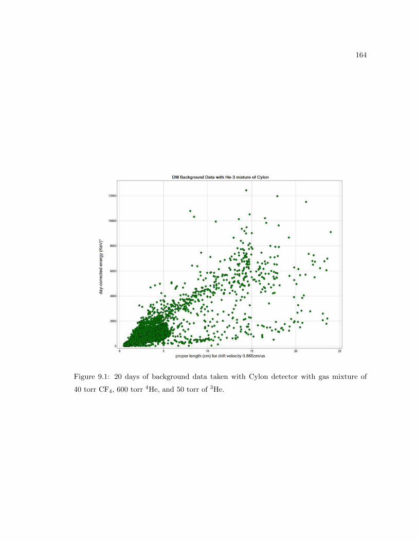
164
Figure 9.1: 20 days of background data taken with Cylon detector with gas mixture of
40 torr CF4, 600 torr 4He, and 50 torr of 3He.

165
Figure 9.2: 20 days of background data taken with Cylon detector with gas mixture of
40 torr CF4, 600 torr 4He, and 50 torr of 3He. Charged particle tracks’ range vs. energy
curves by SRIM simulation are superimposed.
correction process, the actual fiducial volume of the detector has gone down to 7.85 liters.
Fig. 9.2 is the background data scatter plot with the SRIM simulated ion tracks’ range vs.
energy curves superimposed. The smearing of the particle track locations is mainly due to
the non-optimum electron diffusion effect (see Fig. 8.9) because of Cylon’s mechanical con-
straints. Also we are still working on a more sophisticated and precise readout method of
track lengths information. This single scatter plot from the background data run contains
large amount of important information for our Dark Matter research, our detector capa-
bility, and hints for the next generation DMTPC Dark Matter detector. In the following
section, I will identify and discuss particles in this scatter plot by different energy/track
length sectors.

166
(a) (b)
Figure 9.3: (a) Region and (b) sample image of high energy α particle background.
9.2 Particle Identification in Large Energy or Long Track
Region
Fig. 9.3 shows the region of typical high energy α particle background. Those α particles
are emitted from naturally occurring heavy nuclear decays from U/Th/Rn. The α particles
decaying from U/Th have energy range of 4 to 5.5 MeV, and the ones from Rn can go as
high as 6.4 MeV. They may be coming from any material inside the detector, including
copper meshes. In the data analysis, we have reduced the fiducial volume by rejecting any-
thing outside the central 20 cm diameter of the EMCCD view, so it is highly unlikely the
α particle from the wall of the chamber or the field cage rings are included in the scatter
plot presented in this chapter. The high-purity copper we used for the Cylon detector has
reduced the amount of the background α particles by an order of magnitude compared to
a regular grade copper. This type of background can be reduced much more effectively by
using ultra high radio-purity grade material for the detector components.
The next is the charge-one particle background (see Fig. 9.4). Those are the cosmic ray
protons and muons. Also, some protons are coming from the material inside the detector
due to high energy neutron elastic collisions. Having such a low energy threshold, our
detector is capable of triggering and recognizing charge-one muon tracks from cosmic rays

167
(a) (b)
Figure 9.4: (a) Region and (b) sample image of proton/muon background. This image
shows a proton track, but muon tracks look very similar to this.
very well. This type of background can be reduced by placing the detector deep under-
ground. However, those long particle tracks as well as the high energy α particle tracks
can easily be rejected in the data analysis process.
When very high energy neutrons elastically scatter off of a carbon or fluorine nucleus,
these nuclear recoils show very bright and relatively short tracks in the view. Fig. 9.5 is
the example of such nuclear recoil tracks. The estimated energy of the recoil in Fig. 9.5(b)
is approximately 2.5 MeV. These high energy nuclear recoils look very similar to what I
presented earlier in the chapter on testing our prototype Dark Matter detector with a 252Cf
neutron source at MIT (see Sec. 4.1).
9.3 Particle Identification at MeV Region
Fig. 9.6 shows the MeV region of the Cylon background data run with 3He gas mixture.
The fully contained P+T tracks form a local cluster centering at 764 keV of energy given
by thermal neutron absorption events of 3He. The energy resolution is approximately 20 %.
3He gas serves as an excellent calibration source for a TPC. It is very valuable to have the

168
(a) (b)
Figure 9.5: (a) Region and (b) sample image of high energy C or F nuclear recoils induced
by cosmic ray neutrons. The estimated energy of this recoil is approximately 2.5 MeV.
standard 764 keV of energy when identifying other signals we measure. In the data anal-
ysis, we noticed that there are two obvious bands in the partially-contained P+T tracks
region (see Fig. 9.7). These bands are due to the partially missing P+T tracks from the
thermal neutron absorption events occurring at the edge of view or detector. When a triton
side is missing, the location of energy-vs.-length band stays higher in a scatter plot than
that of a proton side missing due to the difference of how much energy is lost per unit length.
Because Cylon detector contains 600 torr of 4He gas, the neutron scattering is increased,
and we expect copious numbers of 4He recoils. Fig. 9.8 shows the typical 4He recoil re-
gion in the scatter plot. Initially, the Cylon detector was always used with the majority
gas mixture ratio of 4He in order to increase the neutron detection sensitivity. Neutrons
being one of the biggest background for a Dark Matter research, we always had an idea of
using a pure CF4 gas. However, along the progress of our research, we experienced several
problems, one of which was the outgassing problem which reduces the electron gain of the
TPC. By increasing the detector gas pressure, we can avoid this problem. We have already
shown that introducing 4He gas into our detector does not create any significant problem
in the search for Dark Matter. Even the fact that background neutrons mimic Dark Matter

169
Figure 9.6: Magnified image of the Cylon Dark Matter background data run scatter plot at
a MeV energy region. This plot focuses on the fully-contained P+T tracks due to thermal
neutron absorption events of 3He.
(a) (b)
Figure 9.7: Partially contained P+T tracks show two bands with (a) triton side, or
(b) proton side missing due to the location of the event occurring near the edge of the
view/detector.

170
(a) (b)
Figure 9.8: (a) Region and (b) sample image of 4He recoils induced by cosmic ray neutrons.
The estimated energy of this recoil is approximately 200 keV.
signals cannot be a big issue because we will need to place our Dark Matter detector deep
underground in order to veto the cosmic ray neutrons. In another words, we can make use
of the 4He gas as a ’double-check’ of the neutron level of the laboratory where the detector
is placed, and if the location is truly neutron free, we should not have any problem using
the gas mixture of CF4 and 4He.
9.4 Particle Identification at Dark Matter Energy Region
In this section, I will discuss our detector’s capability at a low energy region where the
expected Dark Matter signals would be found. Fig. 9.9 shows the low energy region of this
background run data. Although the energy resolution is not very good, one can clearly
see the separation of the C or F recoil band and 4He recoil band. As I mentioned in the
previous section, when the detector is placed deep underground, most or all of the 4He
recoils seen in this scatter plot will disappear; however, even with some ’neutron leaks’ in
the laboratory, our detector should be able to distinguish the Dark Matter signals from
those of background neutrons once the energy resolution is optimized. At the bottom of
Fig. 9.9, there is another band at very low energy. This is an artifact by γ ray background.

171
Figure 9.9: Magnified image of the Cylon Dark Matter background data run scatter plot
at a low energy region. This plot focuses on the separation of C or F and 4He bands.
Our detector is almost transparent to γ ray background and very seldom triggers to them.
Even if some of the γ ray background is recognized by the track finding algorithm, it is
very easy to reject them as seen in this scatter plot.
Fig. 9.10 shows some sample images of C or F nuclear recoil events induced by cosmic ray
neutrons. Although some of the low energy tracks show ambiguous directionality informa-
tion, once we obtain a large number of data, we will be able to statistically determine the
favored directionality of the signals. The energy of these nuclear recoils is estimated to be
approximately the order of 50-100 keV, and the track length is the order of 1-2 mm. This
is about where we would expect to find Dark Matter induced fluorine recoils be at. For this
preliminary data analysis, we made a Dark Matter region cut at the energy of 250 keV and
range of 3 mm. We also applied a cut of all events below the simulated C range-vs.-energy

172
Figure 9.10: Magnified images of low energy C or F nuclear recoils induced by cosmic ray
neutrons. The energy range of these recoils is estimated to be the order of 50−100 keV.
The track length is 1−2 mm.
curve because it provides a reasonable cut for the F band. Over 391 hours of total live time,
we reached a sensitivity volume of 23 g-days (see Fig. 9.11). We concluded that there were
eleven nuclear recoils detected in the Dark Matter energy region during this background
run. This corresponds to 2.1 g-days per background event. This result should be similar
to a result using a more sophisticated data cut analysis technique.
9.5 Cosmic Ray Neutron Induced Inelastic Recoils and Sum-
mary
In this 20 days background run data, we also identified a few inelastic nuclear collision
events induced by high energy cosmic ray neutrons with the energy of tens to hundreds
of MeV (see Fig. 9.12 and Fig. 9.13). By going through all signals in the scatter plot, we
found the total of seven such C or F inelastic nuclear collision events, which also agrees
with what our calculations expected. Inelastic collision events are very rare simply be-
cause the neutron cross section is so much lower than elastic collisions (see Fig. 4.17(a) and
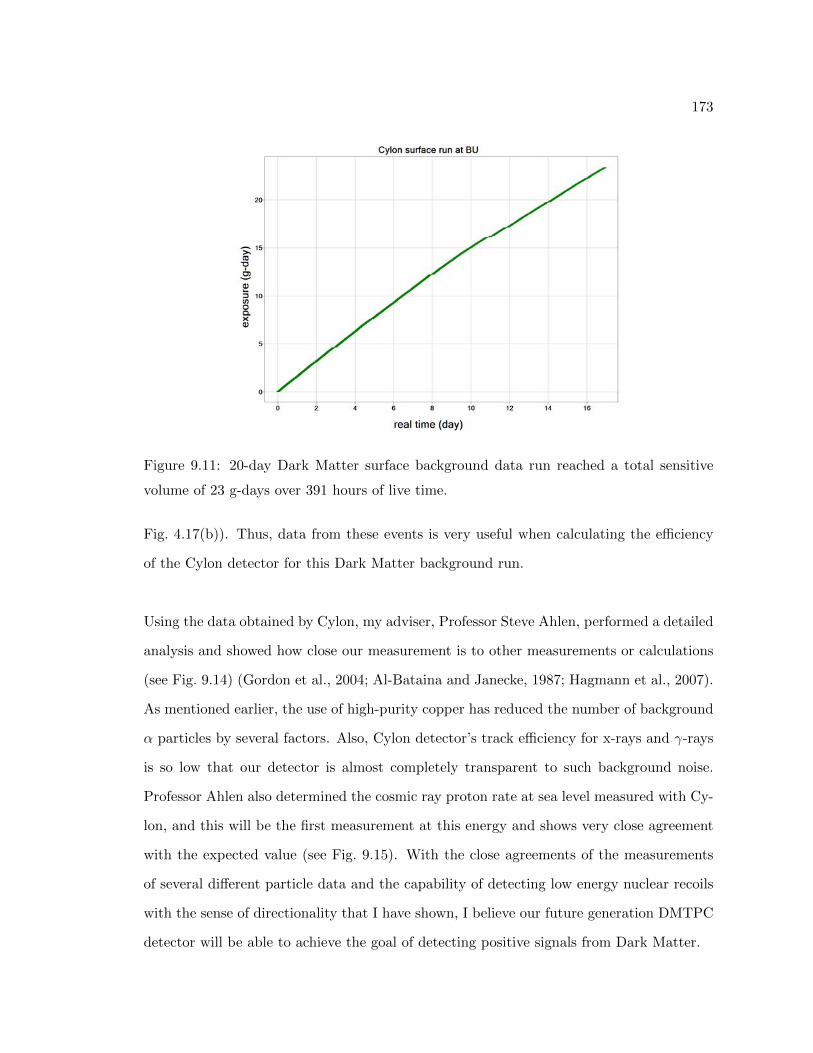
173
Figure 9.11: 20-day Dark Matter surface background data run reached a total sensitive
volume of 23 g-days over 391 hours of live time.
Fig. 4.17(b)). Thus, data from these events is very useful when calculating the efficiency
of the Cylon detector for this Dark Matter background run.
Using the data obtained by Cylon, my adviser, Professor Steve Ahlen, performed a detailed
analysis and showed how close our measurement is to other measurements or calculations
(see Fig. 9.14) (Gordon et al., 2004; Al-Bataina and Janecke, 1987; Hagmann et al., 2007).
As mentioned earlier, the use of high-purity copper has reduced the number of background
α particles by several factors. Also, Cylon detector’s track efficiency for x-rays and γ-rays
is so low that our detector is almost completely transparent to such background noise.
Professor Ahlen also determined the cosmic ray proton rate at sea level measured with Cy-
lon, and this will be the first measurement at this energy and shows very close agreement
with the expected value (see Fig. 9.15). With the close agreements of the measurements
of several different particle data and the capability of detecting low energy nuclear recoils
with the sense of directionality that I have shown, I believe our future generation DMTPC
detector will be able to achieve the goal of detecting positive signals from Dark Matter.

174
(a) (b)
Figure 9.12: (a) Actual viewing size and (b) magnified and color-emphasized image of a
sample C or F inelastic collision events.
(a) (b)
Figure 9.13: (a) Actual viewing size and (b) magnified and color-emphasized image of a
sample C or F inelastic collision events.

175
Figure 9.14: Cylon measurement of particle rate and comparison to other measurements
or calculations. This analysis has been performed by my adviser, Professor Steve Ahlen.

176
Figure 9.15: Cylon measurement of cosmic ray proton at sea level. The green dot indicates
the Cylon measurement. This analysis has been performed by my adviser, Professor Steve
Ahlen (Hagmann et al., 2007).

Chapter 10
Conclusion and Next Goal
I have so far shown and discussed the capabilities of our prototype Dark Matter / Neu-
tron detectors. During last four years of my graduate study and research, we have made
numbers of progresses refining the DMTPC detection technique. Among all the difficult
challenges in the Dark Matter research, I believe the two most important detector capa-
bilities are achieving directionality sensitivity and a low enough energy threshold with the
positive identification of signals above background. Once we understand these aspects of
our detector, we can scale up the detector volume to be in a competitive Dark Matter
detection region.
10.1 Current Status of DMTPC Collaboration
We are currently demonstrating and quantifying our Dark Matter detector’s capability in
the mine of Waste Isolation Pilot Plant (WIPP) laboratory in Carlsbad, New Mexico. The
laboratory area is located about 650m below the surface, which is equivalent to 2,300 m.w.e.
Furthermore, there is a thick salt layer above the laboratory space (see Fig. 10.1). The
expected neutron flux is on the order of 300 /m2/day, which is roughly 2,600 times less
than the typical sea-level locations. The expected muon flux is also as low as 0.1 /m2/min,
which is five orders of magnitude less than that at sea level. This location would be perfect
177

178
(a) (b)
Figure 10.1: (a) The geological information of WIPP. (b) The image of the basement
laboratory area (WIPP).
to quantify our prototype detector for the background study. One of our goals is to make
our detector background free and, in order to do so, we need to understand and quantify
our detector completely in a low background environment like the one at WIPP.
Once we have acquired a sufficient amount of data at the WIPP for the background study
of our prototype Dark Matter detector, our next goal is to build a 1 m3 Dark Matter
detector with all the skills and knowledge we have learnt from our prototype detectors.
The Dark Matter Time Projection Chamber (DMTPC) collaboration group has recently
been awarded $560,000 from the U.S. Department of Energy in order to accelerate our
experiment into the next phase, which is to build a 1 m3 detector.
10.2 1 m3 Dark Matter Detector
10.2.1 Sensitivity and Limits
Under the assumption of zero background level for a 1 m3 DMTPC Dark Matter detector,
the expected sensitivity limit is described in the exclusion plot (see Fig. 10.2(a)). The solid

179
(a) (b)
Figure 10.2: (a) The expected sensitivity (90 % C.L.) of the DMTPC detector to a spin-
dependent WIMP scattering on protons. The dashed lines show the best published limits.
The colored areas show the allowed regions from the MSSM calculations (Sciolla, 2009).
(b) The exclusion limit plot with DMTPC’s 10L surface run at MIT (Battat, 2010).
line with ”DMTPC 0.1 kg-y” is the sensitivity limit that the DMTPC 1 m3 detector would
reach over a data-taking period of 1 year. The region covered in light blue is the estimation
by MSSM of the sensitivity required in order to detect Dark Matter particles. Once the
quality of the next generation DMTPC 1 m3 Dark Matter detector is verified, scaling up
will not be difficult. Once we reach the sensitivity of 100 kg-y, we do expect to be able to
exclude a large amount of the Dark Matter limit area expected by the theory unless our
detector catches positive directional signals from the WIMPs.

180
10.2.2 Design
During the last four years of the R&D phase, we have tried to pursue constant target gas
quality. In order to achieve this goal, we used vacuum chambers as detector bodies. In this
way, we could pump out the chamber down to high-vacuum pressure and clean the detector
before introducing the target gas. Over the years, we learned that no matter how clean we
prepare the chamber before use, outgassing contamination is unavoidable, and we always
had to deal with the electron gain change over time because of the gas purity level. Among
all the contaminants, in particular we need to avoid water and oxygen in the DMTPC
detectors. Lately, we have begun studying how to control the water level of a chamber,
and from the positive outcome of the constant gain level over time with the use of gas
purifier (see Sec. 8.4.2), we have started thinking that our future generation detector will
be equipped with a gas circulation and filtration function, and we may not need expensive
vacuum chambers anymore. This will give us a great deal of freedom in designing the next
generation DMTPC Dark Matter detector, not only because of the freedom in dimensions,
but also we can cut down the cost of building one.
The next improvement we will need is the use of large surface PMTs. As I discussed in
Sec. 6.2.3, the optical readout of particle tracks’ energies may not be the most optimum
because of the unavoidable electron diffusion effect. Although it depends on the drift elec-
tric field and the length of the drift region, it is guaranteed that electrons from the ion
tracks will diffuse in the transverse direction when they have to travel a long distance in
the electron drift region. PMT photon counts, on the other hand, do no depend on the
concentration of the electrons. Diffused or not, PMT signals will be more or less uniform
for the given energy of the traveling particles in the detector. With the great degree of
freedom in the detector design I mentioned above, it will be necessary to use large surface
PMTs for the DMTPC’s next generation 1 m3 Dark Matter detector.
Finally, our next generation Dark Matter detector must be equipped with flat and smooth

181
Figure 10.3: A preliminary drawing of the next generation DMTPC 1 m3 Dark Matter
detector (Inglis, 2010). An array of EMCCDs and PMTs looking down the electron drift
region through a glass and field-shaping cage rings. We can construct such a detector in
any dimension or orientation.
surface amplification stages. As we have learned, it is very important to achieve these
goals, or there will be a resulting fluctuation of the electron gain, which is not acceptable
in a Dark Matter detector. Prior to my joining the group, GEMs (Gas Electron Multipier)
were considered for use as the amplification stage. However, at that early stage in the
research, the group was still struggling with sparking problems. Because a single spark
ruins a GEM board, the use of GEMs was dismissed. Now that we better understand
the sparking, it may be a good idea to once again consider the use of GEMs to reach
the desired combination of electron gain and uniformity. Another possibility would be the
use the electron amplification stages of the MicroMegas (MicroMEsh GAseous Structure).
A micromesh is separated by a smooth surface metal with high-insulating ’posts’, and it
creates an uniform electron amplification region.
Fig. 10.3 presents a conceptual image of DMTPC’s next generation 1 m3 Dark Matter de-

182
(a) (b)
Figure 10.4: (a) An array of 1 m3 conceptual DMTPC detectors in order to increase the
fiducial volume. (b) The array of the detectors will be fitted inside a shipping cargo so
that the whole detector becomes ’portable’ (Inglis, 2010).
tector. Both EMCCDs and PMTs will form an array of the detector ’eyes’. EMCCDs will
be used to detect the 2D projected track length of the traveling particles in the detector,
and PMTs will offer both the energy and vertical components of the particle tracks. The
gas inside the detector will be circulated through a filtration system, so the detector will
no longer need to be qualified as a vacuum chamber. Also, there are no constraints on a
dimension or orientation in constructing such a detector either. One more point I can add
to it is the manufacturability and scalability of the detector.
10.3 100 m3 Dark Matter Detector
Above a 1 m3 detector design, the cost of the detector becomes a very important part of
the detector expansion. If our next generation 1 m3 DMTPC detector becomes easily man-
ufacturable, rather than designing and constructing a single huge Dark Matter detector,
building an array of such 1 m3 detectors in our conceptual design will be a much better idea
in scaling up the detector’s fiducial volume. Thus, we can avoid the difficult task of scaling

183
up the inner TPC system such as an anode plane. Fig. 10.4 shows the conceptual images
of an array of 1 m3 detector in order to scale up our sensitivity. In this way, the array
of the DMTPC detectors can also be ’portable’ by fitting them inside a regular shipping
cargo (see Fig. 10.4(b)). This also means that the detectors can be transported without
much difficulty.
I was recently rewarded with the honor of a new position as a post-doctoral researcher in
the DMTPC collaboration, and as one of the starting members of this Dark Matter exper-
iment group, I have witnessed and contributed to the great progress of our Dark Matter
research.

Bibliography
S. Ahlen. A background-free direction-sensitive neutron detector. In Advancements in
Nuclear Instrumentation, Measurement Methods and their Applications, June 2009.
S. Ahlen. Time-projection-chambers with optical readout for dark matter, double beta
decay, and neutron measurements. International Journal of Modern Physics A, 25(24):
4525–4575, 2010.
B. Al-Bataina and J. Janecke. Alpha-particle emission fromcontaminants in counter ma-
terials. Nuclear Instruments and Methods in Physics Research A, 255:512–517, 1987.
J. Alcaraz, D. Alvisi, B. Alpat, G. Ambrosi, H. Anderhub, and L. Ao et al. Search for
antihelium in cosmic rays. Physics Letters B, 461:387–396, 1999.
V.V. Alekseenko, D.D. Dzhappuev, V.A. Kozyarivsky, A.U. Kudzhaev, V.V. Kuzminov,
O.I. Mikhailova, and Yu.V. Sten’kin. Analysis of variations in the thermal neutron flux
at an altitude of 1700 m above sea level. Bulletin of the Russian Academy of Sciences:
Physics, 71(7):1047–1050, 2007.
V.V. Alekseenko, Yu.M. Gavrilyuk, D.M. Gromushkin, D.D. Dzhappuev, A.U. Kudzhaev,
V.V. Kuzminov, O.I. Mikhailova, Yu.V. Stenkin, and V.I. Stepanov. Correlation of
variations in the thermal neutron flux from the earth’s crust with the moon’s phases and
with seismic activity. Physics of the Solid Earth, 45(8):709–718, 2009.
AndorTM Technology. Technical Specification, ixonEM +888 (back-illuminated) edition,
September 2008.
184

185
E. Aprile, K. Arisaka, F. Arneodo, A. Askin, L. Baudis, A. Behrens, K. Bokeloh, E. Brown,
J. M. R. Cardoso, B. Choi, D. B. Cline, S. Fattori, A. D. Ferella, K.-L. Giboni, A. Kish,
C. W. Lam, J. Lamblin, R. F. Lang, K. E. Lim, J. A. M. Lopes, T. Marrodan Undagoitia,
Y. Mei, A. J. Melgarejo Fernandez, K. Ni, U. Oberlack, S. E. A. Orrigo, E. Pantic,
G. Plante, A. C. C. Ribeiro, R. Santorelli, J. M. F. dos Santos, M. Schumann, P. Shagin,
A. Teymourian, D. Thers, E. Tziaferi, H. Wang, and C. Weinheimer. First dark matter
results from the xenon100 experiment. Phys. Rev. Lett., 105(13):131302, Sep 2010. doi:
10.1103/PhysRevLett.105.131302.
J. Battat. Directional detection of dark matter with dmtpc. In PCTS Workshop on Dark
Matter, November 2010.
C.L. Bennett, M. Halpern, G. Hinshaw, N. Jarosik, A. Kogut, M. Limon, S.S. Meyer,
L. Page, D.N. Spergel, G.S. Tucker, E. Wollack, E.L. Wright, C. Barnes, M.R. Grea-
son, R.S. Hill, E. Komatsu, M.R. Nolta, N. Odegard, H.V. Peiris, L. Verde, and J.L.
Weiland. First-year wilkinson microwave anisotropy probe (wmap) observations: Pre-
liminary maps and basic results. The Astrophysical Journal Supplement Series, 148(1):
1–27, 2003.
R. Bernabei, P. Belli, F. Cappella, R. Cerulli, and C.J. Dai et al. First results from
DAMA/LIBRA and the combined results with DAMA/NaI. European Physical Journal
C, 56:333–355, 2008.
G. Bertone, D. Hooper, and J. Silk. Particle Dark Matter: evidence, candidates and
constraints. Physics Reports, 405:279–390, 2005.
T. Caldwell, A. Roccaro, T. Sahin, D. Dujmic H. Yegoryan, S. Ahlen, J. Battat, P. Fisher,
S. Henderson, A. Kaboth, G. Kohse, R. Lanza, J. Lopez, J. Monroe, G. Sciolla,
N. Skvorodnev, H. Tomita, R. Vanderspek, H. Wellenstein, and R. Yamamoto. Trans-
port properties of electrons in CF4. arXiv/0905.2549v1, Physics Instrumentation and
Detectors, 2009.

186
S. Chang, G.D. Kribs, D. Tucker-Smith, and N. Weiner. Inelastic Dark Matter in light of
DAMA/LIBRA. Physical Review D, 79(4):043513, 2009.
L.G. Christophorou, J.K. Olthoff, and M.V.V.S. Rao. Electron interactions with CF4. The
Journal of Physical Chemical Reference Data, 25:1341–1388, 1996.
D. Clowe, M. Bradac, H. Gonzales, and M. Markevitch. A direct empirical proof of the
existence of Dark Matter. The Astrophysical Journal, 648:L109–L113, 2006.
Y. Cui, D.E. Morrissey, D. Poland, and L. Randall. Candidates for inelastic Dark Matter.
Journal of High Energy Physics, 2009(05):076, 2009.
A.K. Drukier, K. Freese, and D. N. Spergel. Detecting cold Dark-Matter candidates.
Physical Review D, 33(12):3495–3508, 1986.
D. Dujmic, H. Tomita, M. Lewandowska, S. Ahlen, P. Fisher, S. Henderson, A. Kaboth,
G. Kohse, R. Lanza, J. Monroe, A. Roccaro, G. Sciolla, N. Skvorodnev, R. Vanderspek,
H. Wellenstein, and R. Yamamoto. Observation of the ’head-tail’ effect in nuclear recoils
of low-energy neutrons. Nuclear Instruments and Methods in Physics Research A, 584:
327–333, 2008.
Eastman Kodak Company. Performance specification.
http://www.kodak.com/global/en/business/ISS/Products/, October 2010.
M.M.F.R. Fraga, F.A.F. Fraga, S.T.G. Fetal, L.M.S. Margato, R. Ferreira Marques, and
A.J.P.L. Policarpo. The GEM scintillation in He-CF4, Ar-CF4, Ar-TEA and Xe-TEA
mixtures. Nuclear Instruments and Methods in Physics Research A, 504:88–92, 2003.
K. Freese, J. Frieman, and A. Gould. Signal modulation in cold-Dark-Matter detection.
Physical Review D, 37(12):3388–3405, 1988.
J.S. Gainer. Mssm Dark Matter without prejudice. AIP Conference Proceedings, 1200:
1015–1018, 2010.

187
R.J. Gaitskell. Direct detection of Dark Matter. Annual Review of Nuclear and Particle
Science, 54:315–359, 2004.
M. S. Gordon, P. Goldhagen, K. P. Rodbell, T. H. Zabel, H. H. K. Tang, J. M. Clem, and
P. Bailey. Measurement of the flux and energy spectrum of cosmic-ray induced neutrons
on the ground. IEEE Transactions on Nuclear Science, 51:3427, 2004.
C. Hagmann, D. Lange, and D. Wright. Monte carlo simulation of proton-induced cosmic-
ray cascades in the atmosphere. UCRL-TM-229452, Lawrence Livermore National Lab-
oratory, 2007.
Hamamatsu. Performance specification. http://sales.hamamatsu.com/en/products,
October 2010.
A. Inglis. Particle track analysis program. 2008.
A. Inglis. CAD drawing. December 2010.
A. Inglis and Z. Hartwig. ROOT 3D histogram drawing. 2008.
G. Jungman, M. Kamionkowski, and K. Griest. Supersymmetric Dark Matter. Physics
Reports, 267:195–373, 1996.
A. Kaboth, J. Monroe, S. Ahlen, D. Dujmic, S. Henderson, G. Kohse, R. Lanza,
M. Lewandowska, A. Roccaro, G. Sciolla, N. Skvorodnev, H. Tomita, R. Vanderspek,
H. Wellenstein, R. Yamamoto, and P. Fisher. A measurement of photon production in
electron avalanches in CF4. Nuclear Instruments and Methods in Physics Research A,
592:63–72, 2008.
G. Kane and S. Watson. Dark Matter and LHC: what is the connection? Modern Physics
Letters A, 23(26):2103–2123, 2008.
E. Komatsu, K.M. Smith, J. Dunkley, C.L. Bennett, and B. Gold et al. Seven-year wilkin-
son microwave anisotropy probe (wmap1) observations: Cosmological interpretation.
arXiv/1001.4538v3, Physics Instrumentation and Detectors, 2010.

188
Kurt J. Lesker Company. Specification. http://www.lesker.com/, October 2010.
Matheson Tri-Gas. Purification Media - Gases Purified and Specifications, March 2009.
E. Moulin, F. Mayet, and D. Santos. Supersymmetric Dark Matter search via spin-
dependent interaction with 3He. Physics Letters B, 614:143–154, 2005.
National Nuclear Data Center, Brookhaven National Laboratory. Sigma Evaluated Nuclear
Data file (ENDF) Retrieval & Plotting. http://www.nndc.bnl.gov/sigma/, November
2010.
J.F. Navarro, C.S. Frenk, and S.D. White. The structure of cold Dark Matter halos. The
Astrophysical Journal, 462:563–575, 1996.
A. Pansky, A. Breskin, A. Buzulutskov, R. Chechik, V. Elkind, and J. Va’vra. The scintil-
lation of CF4 and its relevance to detection science. Nuclear Instruments and Methods
in Physics Research A, 354:262–269, 1995.
Photonis. Product range and data.
V.C. Rubin, W.K. Ford, and N. Thonnard. Extended rotation curves of high-luminosity
spiral galaxies. IV. systematic dynamical properties, Sa→Sc. The Astrophysical Journal,
225:L107–L111, 1978.
Schneider Optics Inc. C-Mount Objektive / Lenses, standard / 3-ccd edition.
G. Sciolla. Directional detection of Dark Matter. Modern Physics Letters A, 24(23):1793–
1809, 2009.
D.N. Spergel. Motion of the Earth and the detection of weakly interacting massive particles.
Physical Review D, 37(6):1353–1355, 1988.
The Stopping and Range of Ions in Matter. Particle interactions with matter.
http://www.srim.org/, November 2010.
189
The WMAP Science Team. Internal linear combination map.
http://lambda.gsfc.nasa.gov/product/map/current/map images, November
2010.
Thermo Scientific. Neutron Generator model A325 specification.
P. Ullio and M. Kamionkowski. Velocity distributions and annual-modulation signatures
of weakly-interacting massive particles. Journal of High Energy Physics, 3:49, 2001.
H. Wellenstein and A. Dushkin. CAD drawing.
WIPP. U.S. Department of Energy Waste Isolation Pilot Plant.
http://www.wipp.energy.gov/, November 2010.
ZEISS. Xenon arc lamps. http://zeiss-campus.magnet.fsu.edu/articles/, November
2010.
F. Zwicky. Helvetica Physica Acta, 6:110, 1933.
F. Zwicky. On the masses of nebulae and of clusters of nebulae. The Astrophysical Journal,
86(3):217–246, 1937.

Curriculum Vitae
Hidefumi Tomita
Boston University Telephone: 617-353-6088
Physics Department Facsimile: 617/353-9393
590 Commonwealth Avenue E-mail: [email protected]
Boston, Massachusetts 02215 USA
EDUCATION
• January 2011, Ph.D. Physics, Boston University, Boston, MA
Advisor: Steven P. Ahlen
Thesis: Detector development for direction-sensitive Dark Matter research.
•May 2004, B.S., Physics with specialization in Astrophysics, University of California, San
Diego, CA
TEACHING EXPERIENCE
• 2004-2006, Boston University, Boston, MA. Teaching assistant in Modern Physics
AWARDS
• 2009, Alvaro Roccaro Memorial Prize in recognition of an outstanding achievement
in physics, Physics Department, Boston University.
190

191
• 2009, Office of Technology Development Award from Boston University Science and
Engineering Day, Boston University.
• 2009, ”Pass” on the Physics Department preliminary oral exam, Physics Department,
Boston University.
• 2006, Chairman Book Award in recognition of excellence in teaching, Physics De-
partment, Boston University.
• 2005, Chairman Book Award in recognition of excellence in teaching, Physics De-
partment, Boston University.
• 2005, ”Pass” on the Physics Department written comprehensive exam, Physics De-
partment, Boston University.
Languages
• Japanese: mother tongue.
• English: fluent in writing and speaking.
RESEARCH PAPERS
1. A. Rocarro, H. Tomita, S. Ahlen, D. Avery, A. Inglis, J. Battat, D. Dujmic, P.
Fisher, S. Henderson, A. Kaboth, G. Kohse, R. Lanza, J. Monroe, G. Sciolla, N.
Skvorodnev, H. Wellenstein, R. Yamamoto. ”A background-free direction-sensitive
neutron detector,” Nuclear Instruments and Methods in Physics Research Section A
608, 2, 305-309 (2009).
2. D. Dujmic, H. Tomita, M. Lewandowska, S. Ahlen, P. Fisher, S. Henderson, A.
Kaboth, G. Kohse, R. Lanza, J. Monroe, A. Roccaro, G. Sciolla, N. Skvorodnev, R.
Vanderspek, H. Wellenstein, R. Yamamoto. ”Observation of the ”head-tail” effect in
nuclear recoils of low-energy neutrons,” Nuclear Instruments and Methods in Physics
Research Section A 584, 327-333 (2008).

192
3. A. Kaboth, J. Monroe, S. Ahlen, D. Dujmic, S. Henderson, G. Kohse, R. Lanza, M.
Lewandowska, A. Roccaro, G. Sciolla, N. Skvorodnev, H. Tomita, R. Vanderspek,
H. Wellenstein, R. Yamamoto, P. Fisher ”A measurement of photon production in
electron avalanches in CF4,” Nuclear Instruments and Methods in Physics Research
Section A 592, 63-72 (2008).