CLIMATEREADYBOSTON

Climate Change and Sea Level Rise Projections for Boston

The Boston Research Advisory Group Report

JUNE 1, 2016

CLIMATE READY BOSTON | CLIMATEREADY.BOSTON.GOV | #CLIMATEREADYBOSTON

CLIMATEREADYBOSTON

City of BostonMayor Martin J. Walsh

The Green Ribbon Commission

The Barr Foundation

The Sherry and Alan Leventhal Family Foundation

The Boston Foundation

The Boston Research Advisory Group would like to acknowledge the generous support of the following organizations in making this project possible:

This report was prepared for the Climate Ready Boston project, an initiative led by the City of Boston in partnership

with the Green Ribbon Commission.

The goal of Climate Ready Boston is to generate solutions for resilient buildings, neighborhoods, and infrastructure

to help Boston and its metro region prosper in the face of long-term climate change impacts.

Cover photo courtesy of Bud Ris

We would like to thank the following panel of experts for reviewing the BRAG report.

Robin Bell, Columbia UniversityIndrani Ghosh, Kleinfelder

Eddy Moors, Alterra Wageningen University and VU University AmsterdamAnji Seth, University of Connecticut

Geoffrey Trussell, Northeastern UniversityRichard Vogel, Tufts University

Michael Wehner, Lawrence Berkeley National LaboratoryDonald Wuebbles, University of Illinois

Thank you to the copyediting, design and printing teams at The Ink Spot.

Climate Change and Sea Level Rise Projections for Boston

The Boston Research Advisory Group Report

Management Team

Ellen Douglas, University of Massachusetts Boston, Ellen.Douglas@umb.edu

Paul Kirshen, University of Massachusetts Boston, Paul.Kirshen@umb.edu

Robyn Hannigan, University of Massachusetts Boston, Robyn.Hannigan@umb.edu

Rebecca Herst, University of Massachusetts Boston, Rebecca.Herst@umb.edu

Avery Palardy, University of Massachusetts Boston, Avery.Palardy001@umb.edu

Sea Level Rise

Robert DeConto, University of Massachusetts Amherst, Team Leader

Duncan FitzGerald, Boston University

Carling Hay, Harvard University

Zoe Hughes, Boston University

Andrew Kemp, Tufts University

Robert Kopp, Rutgers University

Coastal Storms

Bruce Anderson, Boston University, Team Leader

Zhiming Kuang, Harvard University

Sai Ravela, Massachusetts Institute of Technology

Jonathan Woodruff, University of Massachusetts Amherst

Extreme Precipitation

Mathew Barlow, University of Massachusetts Lowell, Team Leader

Mathias Collins, NOAA

Art DeGaetano, Cornell University

C. Adam Schlosser, Massachusetts Institute of Technology

Extreme Temperatures

Auroop Ganguly, Northeastern University, Team Leader

Evan Kodra, risQ Company

Matthias Ruth, Northeastern University

The scientific results and conclusions, as well as any views or opinions expressed herein, are those of the author(s) and do not necessarily reflect those of NOAA or the Department of Commerce.

A. Introduction ......................................................................................................................................21. The need for a climate consensus ...................................................................................................................22. Risk factors evaluated in the report .................................................................................................................23. Process for reaching consensus ........................................................................................................................24. Process for updating the BRAG projections in the future ..........................................................................3

B. A Brief Primer on Climate Scenarios ...........................................................................................31. Understanding greenhouse gas (GHG) emissions scenarios ..................................................................32. How GHG emissions scenarios are used ........................................................................................................53. Climate change projections used in this report ..........................................................................................5

C. BRAG Findings ...............................................................................................................................61. Sea Level Rise ..........................................................................................................................................................6

a. Keyfindings .....................................................................................................................................................6b. Reviewofexistingscience ............................................................................................................................. 6c. Projections ........................................................................................................................................................ 9d. Openquestionsanddatagaps ................................................................................................................. 14

2. Coastal Storms ......................................................................................................................................................14a. Keyfindings .................................................................................................................................................... 14b. Reviewofexistingscience .......................................................................................................................... 15c. Projections ...................................................................................................................................................... 17d. Openquestionsanddatagaps ................................................................................................................. 18e. Jointfloodingbetweenrain-andstormsurge-drivenflooding ............................................................. 19

3. Extreme Precipitation .........................................................................................................................................21a. Keyfindings .................................................................................................................................................... 21b. Reviewofexistingscience ........................................................................................................................... 21c. Projections ...................................................................................................................................................... 23d. Openquestionsanddatagaps ................................................................................................................. 26

4. Extreme Temperatures .......................................................................................................................................27a. Keyfindings ....................................................................................................................................................27b. Reviewofexistingscience .......................................................................................................................... 27c. Projections ......................................................................................................................................................29d. Discussionanddatagaps ...........................................................................................................................33

D. Conclusion ...................................................................................................................................34

E. Appendix A ..................................................................................................................................39

F. References ...................................................................................................................................44Introduction: .................................................................................................................................................................. 44Sea Level Rise: ............................................................................................................................................................... 45Coastal Storms: ..............................................................................................................................................................47Extreme Precipitation: .................................................................................................................................................49Extreme Temperatures: ...............................................................................................................................................51Appendix A .................................................................................................................................................................... 54

Table of Contents

Sea Level Rise key findings ............................................................................................................................... 6Coastal Storms key findings .............................................................................................................................14Extreme Precipitation key findings ................................................................................................................ 21Extreme Temperatures key findings ............................................................................................................... 27

1

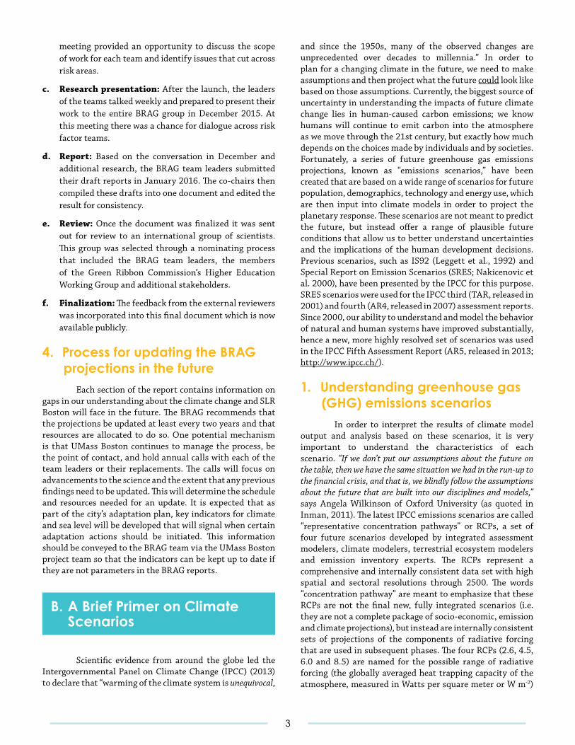
While there were already many ongoing activities prior to October 2012, Superstorm Sandy spurred Boston and surrounding communities to accelerate planning and action on climate change resilience. This activity has led to a number of vulnerability assessment and adaptation strategy reports which include, but are not limited to, Preparing for the Rising Tide (Douglas, 2013), Greenovate Boston Climate Action Plan (Spector, 2013), The Boston Water and Sewer Commission Master Plan (BWSC, 2015), and The City of Cambridge Climate Change Vulnerability Assessment (City of Cambridge, 2015). The climate projections used in each of these reports are specific to the sites, sectors and time periods of interest and not necessarily consistent with one another. Hence, it is unclear which projections and results are the most relevant and useful to the City of Boston proper. To address this issue, the Boston Research Advisory Group (BRAG) was established in 2015 to develop a consensus on the possible climate changes and sea level rise (SLR) that the City of Boston will face in the future by 2030, 2050, 2070, and 2100; consensus on the climate projections is necessary because it is important that the results of this study are not disputed. The BRAG was overseen by the UMass Boston project team.

2. Risk factors evaluated in the report

This report summarizes the current understanding of the local factors that influence Boston’s future exposure to climate change risks. The following four risk factors were considered most relevant to Boston and are therefore evaluated in this report: sea-level rise, extreme precipitation, coastal storms and extreme temperatures. For each risk factor, a team of scientific experts, comprised of a team leader and three or more team members, was selected to evaluate and summarize the available information contained in both grey (reports, conference proceedings and the like) and peer-reviewed literature. Each team met independently between October 2015 and January 2016, and team leaders had regular teleconferences with the UMass Boston project team to keep them apprised of progress and to help overcome problems that were encountered. The process for reaching consensus is outlined in the next section.

3. Process for reaching consensus

a. Building the group: To build the BRAG, the co-chairs developed a list of faculty at institutions around Mas-sachusetts who specialize in coastal storms, tempera-tures, precipitation and sea level rise. At the same time, the BRAG project manager researched faculty at local schools to ensure that there were no oversights. Some scientists were immediately identified as potential risk team leaders. A conversation with these experts fol-lowed to get their input on additional invitations.

b. Kickoff: Once the teams were finalized, the BRAG was launched at a kickoff meeting in late October 2015. This

A. Introduction

1. The need for a climate consensus

On January 20, 2016, both NASA and NOAA announced that 2015 was the warmest year on record globally, beating the previous record set in 2014, by 0.29°F (Chapel, 2015). In fact, the fifteen warmest years since 1880 have all occurred in the seventeen years 1998 to 2015 (NOAA, 2015a). For Boston, December 2015 was the warmest on record and winter 2015-2016 was the second warmest on record (National Weather Service, 2015). Within the scientific community, the effect of human activities on the climate is evident. As the Intergovernmental Panel on Climate Change (IPCC; www.ipcc.ch) concluded in 2013, “Human influence on the climate system is clear, and recent anthropogenic emissions of greenhouse gases are the highest in history. Recent climate changes have had widespread impacts on human and natural systems.” (IPCC, 2013). Advances in both scientific understanding and computer modeling have resulted in refined projections for future climate impacts, and in some cases, a more probabilistic, risk-based approach. These scientific advances are bittersweet, however. On the one hand, we have increased confidence of both the underlying causes and model estimates of our changing global climate (NOAA, 2015b). On the other hand, with this increased confidence has come greater concern and motivation for action at local and community scales. Local action requires local information. While advances in climate models continue, the granularity (in space and time) of these model outputs does not directly map against local concerns. Thus, the climate community must meet these needs while reconciling irreducible uncertainties – and more and more by providing probabilistic information of all outcomes that present a threat.

The IPCC was established by the  United Nations Environment Programme and the  World Meteorological Organization  in 1988 and has provided the world with a series of scientific assessments of the current state of knowledge about climate change and the potential environmental and socio-economic impacts, beginning with the First Assessment Report in 1990 (IPCC, 1990). The IPCC reviews and assesses the most recent scientific, technical and socio-economic information produced worldwide relevant to the understanding of climate change; it does not conduct research or monitor climate-related data or parameters (IPCC, 2000). However, the results presented by the IPCC are relevant at continental to regional scales and cannot be directly applied at the level of a municipality for each town or city. As a result, site-specific projects and research must be carried out to determine local vulnerabilities.

2

meeting provided an opportunity to discuss the scope of work for each team and identify issues that cut across risk areas.

c. Research presentation: After the launch, the leaders of the teams talked weekly and prepared to present their work to the entire BRAG group in December 2015. At this meeting there was a chance for dialogue across risk factor teams.

d. Report: Based on the conversation in December and additional research, the BRAG team leaders submitted their draft reports in January 2016. The co-chairs then compiled these drafts into one document and edited the result for consistency.

e. Review: Once the document was finalized it was sent out for review to an international group of scientists. This group was selected through a nominating process that included the BRAG team leaders, the members of the Green Ribbon Commission’s Higher Education Working Group and additional stakeholders.

f. Finalization: The feedback from the external reviewers was incorporated into this final document which is now available publicly.

4. Process for updating the BRAG projections in the future

Each section of the report contains information on gaps in our understanding about the climate change and SLR Boston will face in the future. The BRAG recommends that the projections be updated at least every two years and that resources are allocated to do so. One potential mechanism is that UMass Boston continues to manage the process, be the point of contact, and hold annual calls with each of the team leaders or their replacements. The calls will focus on advancements to the science and the extent that any previous findings need to be updated. This will determine the schedule and resources needed for an update. It is expected that as part of the city’s adaptation plan, key indicators for climate and sea level will be developed that will signal when certain adaptation actions should be initiated. This information should be conveyed to the BRAG team via the UMass Boston project team so that the indicators can be kept up to date if they are not parameters in the BRAG reports.

B. A Brief Primer on Climate Scenarios

Scientific evidence from around the globe led the Intergovernmental Panel on Climate Change (IPCC) (2013) to declare that “warming of the climate system is unequivocal,

and since the 1950s, many of the observed changes are unprecedented over decades to millennia.” In order to plan for a changing climate in the future, we need to make assumptions and then project what the future could look like based on those assumptions. Currently, the biggest source of uncertainty in understanding the impacts of future climate change lies in human-caused carbon emissions; we know humans will continue to emit carbon into the atmosphere as we move through the 21st century, but exactly how much depends on the choices made by individuals and by societies. Fortunately, a series of future greenhouse gas emissions projections, known as “emissions scenarios,” have been created that are based on a wide range of scenarios for future population, demographics, technology and energy use, which are then input into climate models in order to project the planetary response. These scenarios are not meant to predict the future, but instead offer a range of plausible future conditions that allow us to better understand uncertainties and the implications of the human development decisions. Previous scenarios, such as IS92 (Leggett et al., 1992) and Special Report on Emission Scenarios (SRES; Nakicenovic et al. 2000), have been presented by the IPCC for this purpose. SRES scenarios were used for the IPCC third (TAR, released in 2001) and fourth (AR4, released in 2007) assessment reports. Since 2000, our ability to understand and model the behavior of natural and human systems have improved substantially, hence a new, more highly resolved set of scenarios was used in the IPCC Fifth Assessment Report (AR5, released in 2013; http://www.ipcc.ch/).

1. Understanding greenhouse gas (GHG) emissions scenarios

In order to interpret the results of climate model output and analysis based on these scenarios, it is very important to understand the characteristics of each scenario. “If we don’t put our assumptions about the future on the table, then we have the same situation we had in the run-up to the financial crisis, and that is, we blindly follow the assumptions about the future that are built into our disciplines and models,” says Angela Wilkinson of Oxford University (as quoted in Inman, 2011). The latest IPCC emissions scenarios are called “representative concentration pathways” or RCPs, a set of four future scenarios developed by integrated assessment modelers, climate modelers, terrestrial ecosystem modelers and emission inventory experts. The RCPs represent a comprehensive and internally consistent data set with high spatial and sectoral resolutions through 2500. The words “concentration pathway” are meant to emphasize that these RCPs are not the final new, fully integrated scenarios (i.e. they are not a complete package of socio-economic, emission and climate projections), but instead are internally consistent sets of projections of the components of radiative forcing that are used in subsequent phases. The four RCPs (2.6, 4.5, 6.0 and 8.5) are named for the possible range of  radiative forcing (the globally averaged heat trapping capacity of the atmosphere, measured in Watts per square meter or W m-2)

3

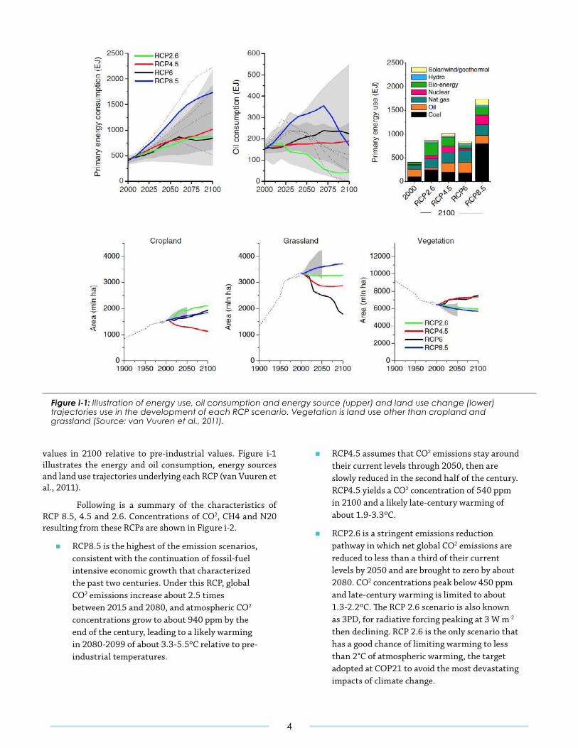
values in 2100 relative to pre-industrial values. Figure i-1 illustrates the energy and oil consumption, energy sources and land use trajectories underlying each RCP (van Vuuren et al., 2011).

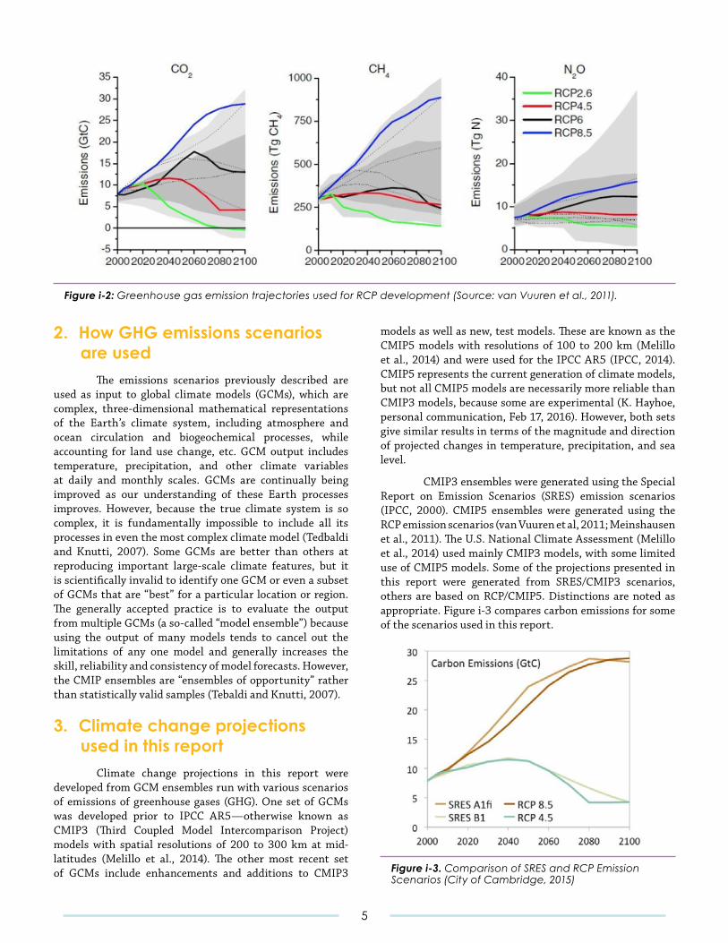
Following is a summary of the characteristics of RCP 8.5, 4.5 and 2.6. Concentrations of CO2, CH4 and N20 resulting from these RCPs are shown in Figure i-2.

■ RCP8.5 is the highest of the emission scenarios, consistent with the continuation of fossil-fuel intensive economic growth that characterized the past two centuries. Under this RCP, global CO2 emissions increase about 2.5 times between 2015 and 2080, and atmospheric CO2 concentrations grow to about 940 ppm by the end of the century, leading to a likely warming in 2080-2099 of about 3.3-5.5ºC relative to pre-industrial temperatures.

■ RCP4.5 assumes that CO2 emissions stay around their current levels through 2050, then are slowly reduced in the second half of the century. RCP4.5 yields a CO2 concentration of 540 ppm in 2100 and a likely late-century warming of about 1.9-3.3ºC.

■ RCP2.6 is a stringent emissions reduction pathway in which net global CO2 emissions are reduced to less than a third of their current levels by 2050 and are brought to zero by about 2080. CO2 concentrations peak below 450 ppm and late-century warming is limited to about 1.3-2.2ºC. The RCP 2.6 scenario is also known as 3PD, for radiative forcing peaking at 3 W m-2 then declining. RCP 2.6 is the only scenario that has a good chance of limiting warming to less than 2°C of atmospheric warming, the target adopted at COP21 to avoid the most devastating impacts of climate change.

Figure i-1:Illustrationofenergyuse,oilconsumptionandenergysource(upper)andlandusechange(lower)trajectoriesuseinthedevelopmentofeachRCPscenario.Vegetationislanduseotherthancroplandand grassland(Source:vanVuurenetal.,2011).

4

2. How GHG emissions scenarios are used

The emissions scenarios previously described are used as input to global climate models (GCMs), which are complex, three-dimensional mathematical representations of the Earth’s climate system, including atmosphere and ocean circulation and biogeochemical processes, while accounting for land use change, etc. GCM output includes temperature, precipitation, and other climate variables at daily and monthly scales. GCMs are continually being improved as our understanding of these Earth processes improves. However, because the true climate system is so complex, it is fundamentally impossible to include all its processes in even the most complex climate model (Tedbaldi and Knutti, 2007). Some GCMs are better than others at reproducing important large-scale climate features, but it is scientifically invalid to identify one GCM or even a subset of GCMs that are “best” for a particular location or region. The generally accepted practice is to evaluate the output from multiple GCMs (a so-called “model ensemble”) because using the output of many models tends to cancel out the limitations of any one model and generally increases the skill, reliability and consistency of model forecasts. However, the CMIP ensembles are “ensembles of opportunity” rather than statistically valid samples (Tebaldi and Knutti, 2007).

3. Climate change projections used in this report

Climate change projections in this report were developed from GCM ensembles run with various scenarios of emissions of greenhouse gases (GHG). One set of GCMs was developed prior to IPCC AR5—otherwise known as CMIP3 (Third Coupled Model Intercomparison Project) models with spatial resolutions of 200 to 300 km at mid-latitudes (Melillo et al., 2014). The other most recent set of GCMs include enhancements and additions to CMIP3

models as well as new, test models. These are known as the CMIP5 models with resolutions of 100 to 200 km (Melillo et al., 2014) and were used for the IPCC AR5 (IPCC, 2014). CMIP5 represents the current generation of climate models, but not all CMIP5 models are necessarily more reliable than CMIP3 models, because some are experimental (K. Hayhoe, personal communication, Feb 17, 2016). However, both sets give similar results in terms of the magnitude and direction of projected changes in temperature, precipitation, and sea level.

CMIP3 ensembles were generated using the Special Report on Emission Scenarios (SRES) emission scenarios (IPCC, 2000). CMIP5 ensembles were generated using the RCP emission scenarios (van Vuuren et al, 2011; Meinshausen et al., 2011). The U.S. National Climate Assessment (Melillo et al., 2014) used mainly CMIP3 models, with some limited use of CMIP5 models. Some of the projections presented in this report were generated from SRES/CMIP3 scenarios, others are based on RCP/CMIP5. Distinctions are noted as appropriate. Figure i-3 compares carbon emissions for some of the scenarios used in this report.

Figure i-2:GreenhousegasemissiontrajectoriesusedforRCPdevelopment(Source:vanVuurenetal.,2011).

Figure i-3.ComparisonofSRESandRCPEmissionScenarios(CityofCambridge,2015)

5

C. BRAG Findings

1. Sea Level Rise

a. Key findings

■ The overall trend in relative sea level rise (RSLR) in Boston between 1921 and 2015 has been about 2.8 mm/yr (0.11 in/yr).

■ Due to the influence of regional-scale processes such as ocean dynamics and the gravitational effect of melting ice sheets, RSLR in Boston will likely exceed the global average throughout the 21st century, regardless of which emissions trajectory is followed.

■ The amount and rate of RSLR in Boston during the first half of the 21st century is nearly independent of emissions. The most likely estimates of RSLR from 2000 to 2050 (associated with exceedance probabilities of 83%, 50%, and 17%) are 19, 32 and 45 cm (7.5, 13 and 18 in), thus a 2050 range of 19 cm to 45 cm (7.5 to 18 in) can be considered, but higher RSLR approaching 75 cm (30 in) is possible.

■ After ~2050 the scenarios diverge sharply, with substantially more RSLR under the higher emissions pathways. Under the highest emissions pathway (RCP8.5), the most likely estimates of RSLR from 2000 to 2100 in Boston are 97, 149 and 226 cm (3.2, 4.9 and 7.4 ft). Under the moderate-emissions RCP4.5 pathway, RSLR estimates from 2000 to 2100 are 74, 111 and 156 cm (2.4, 3.6 and 5.1 ft). Thus a 2100 range of 74 cm to 226 cm (2.5 to 7.4 ft) can be considered.

■ Sea-level rise will not stop in 2100, and because some long-lived infrastructure and land use plans will likely extend into the 22nd century, changes in RSL should be considered beyond 2100. If the high RCP8.5 emission scenario is followed, the rate of RSL rise by the end of the 21st century may be 19-48 mm/yr (0.75-1.9 in/yr), an order of magnitude faster than today, and will continue to accelerate.

■ The accelerating rate of RSLR that will characterize RSL change in Boston during the 21st century will soon make salt-

marsh drowning events more frequent and widespread. Eventually salt marshes such as those located at Quincy, Neponset, and Belle Isle will be converted to tidal flats and sub-tidal bays, because the ecological limits of in situ organic sediment production and the very low suspended sediment concentration in Boston Harbor are insufficient to keep pace with the projected rates of RSL rise.

■ The maximum physically plausible sea-level rise from 2000 to 2100 at Boston was estimated to range from 1.9 m and 3.2 m (6.2 and 10.5 ft) in this analysis. This is substantially more than the maximum RSLR of 2.08 m (6.83 ft) from 2003 to 2100 under the highest emissions scenario reported in a recent study by CZM (2013).

■ RSL rise will increase tidal range, wave energy, and tidal inundation, resulting in increased erosion of existing geomorphic features and existing or planned coastal engineering works such as flood defenses. It will also increase the elevation of coastal storm surges.

b. Review of existing science

1. Definitions Relative sea level (RSL) is the difference in elevation between the sea surface and land surface at a specific place and time (Farrell & Clark, 1976). By convention, the reference time period is a multi-year average; this minimizes the effect of tidal and seasonal cycles, and multi-annual climate variability (e.g. Shennan, Milne, & Bradley, 2012). We use a 19-year period centered on the year 2000 as a baseline, such that negative and positive values denote periods when RSL was either lower or higher than the reference period, respectively. Previous analyses of Boston sea-level trends have used the mid-point (1992) of the 1983-2001 National Tidal Datum Epoch (NTDE) as their reference point. About 3cm (1.2 in) of sea-level rise occurred between 1992 and the 2000 reference point used here. Additionally, between 1990 and 2010, the average rate of sea-level rise at Boston was 5.3 cm (2.1 in) per decade, so RSL in 2015 is about 7.9 cm (3.1 in) above the 2000 reference level. As discussed below, there is considerable annual to decadal variability in RSL. For example, average annual RSL in Boston has varied from the long-term average (over the duration of the tide gauge record since 1921) with 1σ standard deviation of ~±5.8 cm (2.3 in). We note that projections of future RSL are provided specifically for the location of the Boston, MA tide gauge station (#8443970) operated by the National Ocean and Atmospheric Administration (NOAA).

6

2. Processes causing relative sea-level change in Boston

Changes in RSL are caused by multiple, complex, simultaneous processes that vary both spatially and through time (Kopp et al., 2015). As a result, making reliable predictions of future RSL at specific times and locations is difficult. Nonetheless, recent advances in understanding and modeling the dominant processes that control RSL are leading to improved estimates of the potential range of future sea-level change over the next century and beyond, with important implications for coastal planning and management.

a. Thermal expansion and ice-sheet melt Over the 21st century and beyond, RSL in Boston will be affected by several local to regional-scale processes in addition to the projected rise in global mean sea level (GMSL). Over the 20th and early 21st century, the two primary contributors to changes in GMSL have been the thermal expansion of seawater and the loss of land ice. When the ocean warms, the volume of water in the ocean increases, raising GMSL. When land ice melts, water is added to the ocean, which also increases GMSL. Human activity has also altered the Earth’s natural water cycle, leading to additional changes in the mass of the ocean. For example, storage of water on land in reservoirs and behind dams causes RSL to fall, while pumping of water from aquifers for irrigation and consumption ultimately transfers water to the ocean, causing RSL to rise (e.g. Chao, Wu, & Li, 2008; Konikow, 2011; Wada et al., 2012). Over the last two decades, thermal expansion has been responsible for about 40% of global mean sea-level rise, land-ice shrinkage for about 50%, and changes in land water storage for about 10% (Church et al., 2013). Later in this century, land ice on Greenland and Antarctica are expected to play an increasingly important, and likely a dominant role in GMSL rise (Rignot et al., 2011).

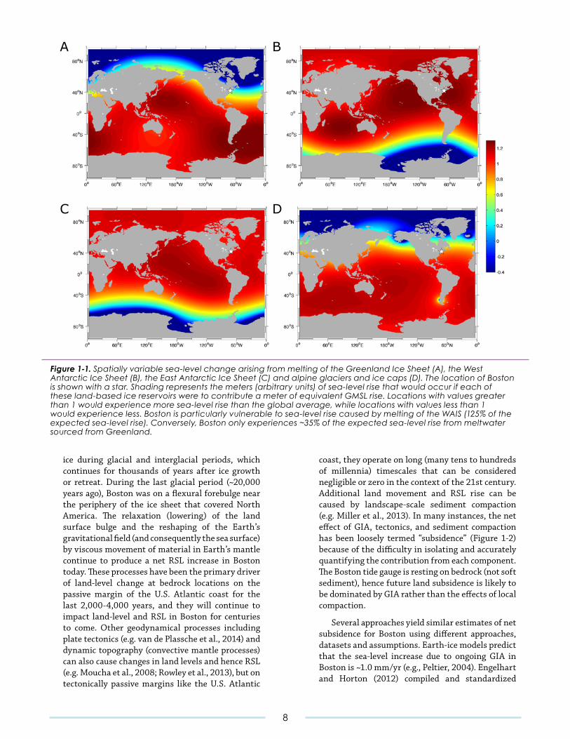
b. Gravitational effect of ice sheet melt The melting of land-based ice does not cause globally uniform sea-level rise. The dispersion of mass, previously concentrated in glaciers and ice sheets, into the ocean changes the Earth’s gravitational field and rotation, and it causes the Earth to deform. As a result, locations near a melting ice sheet experience less sea-level rise than more distant locations (Mitrovica et al., 2001, 2009, 2011). The resulting spatial pattern of sea-level rise driven by a given loss of ice mass from a specific source is shown in Figure 1-1. The implications for Boston are significant, because of Boston’s relative proximity to Greenland and great distance from Antarctica. Boston will experience proportionally less than the global average sea-level rise due to melting of the Greenland Ice Sheet (GIS; about 35%

of the global mean sea-level signal), but more than the global average for sea-level rise due to mass loss on the West Antarctic Ice Sheet (WAIS; about 125%) or the East Antarctic Ice Sheet (EAIS; about 105%).

Smaller, globally distributed alpine glaciers and ice caps (GIC) also produce non-uniform changes in sea-level, but their total potential contribution to long-term sea-level rise (~0.6m) is small relative to the potential sea-level rise from retreat of continental-scale ice sheets on Greenland (~7m), West Antarctica (~5m), and East Antarctica (~53m). Previous efforts to project RSL change in Boston (CZM, 2013; Bosma et al., 2015) did not include the non-uniform effects of ice sheet and glacier mass loss and may, therefore, substantially over- or underestimate sea-level rise depending on the source of meltwater. Most importantly for Boston, if the WAIS becomes the largest source of glacial meltwater to the global ocean in the 21st century, Boston will experience a sea-level rise ~125% of the global mean. Not accounting for this effect could lead to a substantial underestimate of 21st century sea-level change.

c. Ocean dynamics Changes in the location and strength of ocean currents and/or prevailing winds, as well as in the distribution of heat and salt in the ocean, can induce “dynamic sea-level” changes. Along the U.S. Atlantic coast at locations north of Cape Hatteras, NC (including Boston), a regional-scale dynamic sea-level rise can be caused by a reduction in the strength of the Gulf Stream and/or a migration of the current toward the coastline (e.g. Ezer et al., 2013; Kopp, 2013; Sallenger et al., 2012; Yin and Goddard, 2013; Yin et al., 2009). A reduction in the strength of the Gulf Stream system is projected by many climate models for the 21st century (Yin, 2012; Yin and Goddard, 2013), largely as a response to warming and freshening of North Atlantic surface waters and a weakening of the Atlantic Meridional Overturing Circulation. Persistent trends in the North Atlantic Oscillation, the dominant mode of North Atlantic inter-annual climate variability, can also have an effect via the influence of persistent northeasterly wind-stress anomalies on upper ocean (Ekman) transports toward the New England coast (Goddard et al., 2015). Combined with thermal expansion, these ocean dynamical mechanisms have the potential to produce >10 cm (3.9 in) RSL rise along the Massachusetts coast by 2100 (Yin, 2012).

d. Vertical land movement RSL is also affected by changes in the elevations of both the land and sea surfaces due to a process known as glacial isostatic adjustment (GIA; e.g., Peltier, 2004). GIA reflects the response of the solid Earth to the loading and unloading of continental

7

ice during glacial and interglacial periods, which continues for thousands of years after ice growth or retreat. During the last glacial period (~20,000 years ago), Boston was on a flexural forebulge near the periphery of the ice sheet that covered North America. The relaxation (lowering) of the land surface bulge and the reshaping of the Earth’s gravitational field (and consequently the sea surface) by viscous movement of material in Earth’s mantle continue to produce a net RSL increase in Boston today. These processes have been the primary driver of land-level change at bedrock locations on the passive margin of the U.S. Atlantic coast for the last 2,000-4,000 years, and they will continue to impact land-level and RSL in Boston for centuries to come. Other geodynamical processes including plate tectonics (e.g. van de Plassche et al., 2014) and dynamic topography (convective mantle processes) can also cause changes in land levels and hence RSL (e.g. Moucha et al., 2008; Rowley et al., 2013), but on tectonically passive margins like the U.S. Atlantic

coast, they operate on long (many tens to hundreds of millennia) timescales that can be considered negligible or zero in the context of the 21st century. Additional land movement and RSL rise can be caused by landscape-scale sediment compaction (e.g. Miller et al., 2013). In many instances, the net effect of GIA, tectonics, and sediment compaction has been loosely termed “subsidence” (Figure 1-2) because of the difficulty in isolating and accurately quantifying the contribution from each component. The Boston tide gauge is resting on bedrock (not soft sediment), hence future land subsidence is likely to be dominated by GIA rather than the effects of local compaction.

Several approaches yield similar estimates of net subsidence for Boston using different approaches, datasets and assumptions. Earth-ice models predict that the sea-level increase due to ongoing GIA in Boston is ~1.0 mm/yr (e.g., Peltier, 2004). Engelhart and Horton (2012) compiled and standardized

Figure 1-1.Spatiallyvariablesea-levelchangearisingfrommeltingoftheGreenlandIceSheet(A),theWestAntarcticIceSheet(B),theEastAntarcticIceSheet(C)andalpineglaciersandicecaps(D).ThelocationofBostonisshownwithastar.Shadingrepresentsthemeters(arbitraryunits)ofsea-levelrisethatwouldoccurifeachoftheseland-basedicereservoirsweretocontributeameterofequivalentGMSLrise.Locationswithvaluesgreaterthan1wouldexperiencemoresea-levelrisethantheglobalaverage,whilelocationswithvalueslessthan1wouldexperienceless.Bostonisparticularlyvulnerabletosea-levelrisecausedbymeltingoftheWAIS(125%oftheexpectedsea-levelrise).Conversely,Bostononlyexperiences~35%oftheexpectedsea-levelrisefrommeltwatersourcedfromGreenland.

A

DC

B

8

geological RSL reconstructions from the period between 4,000 years ago and 1900 and concluded that the linear rate of RSL rise (~0.7 mm/yr; Figure 1-3) could be entirely attributed to subsidence. Using a global statistical model that included high-resolution geological records, Kopp et al. (2016) found a rate of RSL rise of 0.5 ± 0.1 mm/yr at Wood Island and 0.6 ± 0.1 mm/yr at Revere from 0 to 1700. Kopp et al. (2016) attributed these rates of RSL change to local subsidence and ongoing GIA. A short time series of measurements made by permanent global positioning satellite stations around Boston also estimates that subsidence produces a RSL rise of 0.7 ± 0.2 mm/yr (Karegar et al., submitted). Zervas et al. (2013) processed RSL measurements made at the Boston tide gauge to remove monthly variability caused by oceanographic effects and an assumed rate of global average sea-level rise (1.7 mm/yr; Church and White, 2011). They attributed the residual signal (0.84 mm/yr) in the tide-gauge record to subsidence. Kopp (2013) applied a statistical model to RSL measurements made by a global network of tide gauges to partition local RSL trends into a global component (common to all locations), a regional, linear component (broadly equivalent to an estimate of subsidence), and a regional non-linear component. For Boston, this analysis yields an estimate of RSL rise due to subsidence of 0.8 ± 0.3 mm/yr. Within its uncertainty, this estimate captures the range of estimates from other studies, including GIA modeling and observations. Previous projections of RSL in Boston (e.g., CZM, 2013; Bosma et al., 2015) assumed subsidence resulted in RSL rates of 0.84 mm/yr (based the analysis of Zervas, 2013) and 1.1 mm/yr (based on Kirshen et al., 2008). The convergence of estimates from different sources and approaches suggest that an assumed RSL rate due to subsidence of 0.8 ± 0.3 mm/yr is robust. On the timescale considered here, subsidence at the Boston tide gauge location will be independent of climate change, so this rate and its uncertainty is applied to all of our future projections, regardless of which climate scenario is followed (Figure 1-2).

c. Projections

1. Spatial and temporal scales of RSL projections

Estimating future RSL for specific locations at the local-neighborhood spatial scale and/or for individual years requires consideration of local and annual-scale processes that are not explicitly estimated in our approach or projections (Figure 1-2). As noted above, the Boston tide gauge is situated on bedrock and is therefore not subject to local-scale subsidence. In contrast, much of the city is prone to autocompaction of underlying sediment composed of

fill, providing a potential additional source of RSL rise. The composition, thickness, age and loading history of filled areas is spatially variable and poorly quantified, meaning that detailed geotechnical investigations will be needed to estimate an appropriate adjustment to our sea-level projections for specific neighborhoods or locales. However, we anticipate that the rate of autocompaction will likely be <1 mm/yr and could be approximated as linear over coming decades, provided no significant changes in loading (e.g. new construction).

The projections of RSL provided here are averages across an interval of 19 contiguous years, centered on 2030, 2050, 2070, and 2100. For example, projections for 2050 are the average of the period 2041-2059. RSL may depart from this average for any specific day, season, year, or decade due to a number of processes. Firstly, tide-gauge measurements show substantial “noise” around the overall RSL trend. This variability is caused by short-lived weather patterns that can push water onto or away from the coast (Goddard et al., 2015) and into or out of Boston Harbor. Analysis of multiple tide gauges demonstrates that this variability is generally regional in scale (e.g. Wahl et al., 2013). The Boston tide-gauge record indicates that this contribution to annual RSL was up to ~±5.8 cm for the period since 1921, and that this variability contributed ~±3.3 cm to decadal-average sea level over this time period (Figure 1-3).

Secondly, tides follow annual, monthly, seasonal and multi-annual cycles, and the predicted timing of these cycles will help determine the elevation attained by a particular high tide occurring on top of the projected sea-level rise, and the potential for storm-induced flooding superposed on a specific tidal cycle and projected RSL estimate (see Coastal Storms section). Thirdly, RSL rise will modify the bathymetry of Boston Harbor resulting in an altered tidal range and wave climate. Other factors affecting astronomical and meteorological tidal amplitude include geomorphic evolution of Boston Harbor, sediment dredging, trends in freshwater input from fluvial systems, and the construction of coastal defenses (Figure 1-4). In the future, ongoing hydrodynamic modeling (e.g., Bosma et al., 2015) will be necessary to quantify the influence of these processes on local and annual RSL in and around Boston.

2. Projections of 21st-century relative sea-level change in Boston

Previous studies of RSL change in Boston (e.g., CZM, 2013; Bosma et al., 2015) considered four discrete, future climate scenarios. A limitation of this approach is the “inability to assign likelihood to any particular scenario” (Bosma et al., 2015). With future sea-level scenarios presented as a series of discrete pathways, end users and stakeholders are left to decide which outcomes are the most likely to be realized (e.g., Parris et al., 2012). Furthermore, projections generated by summing multiple and uncertain sea-level contributions often fail to formally propagate uncertainty into the analysis. Previous analyses

9

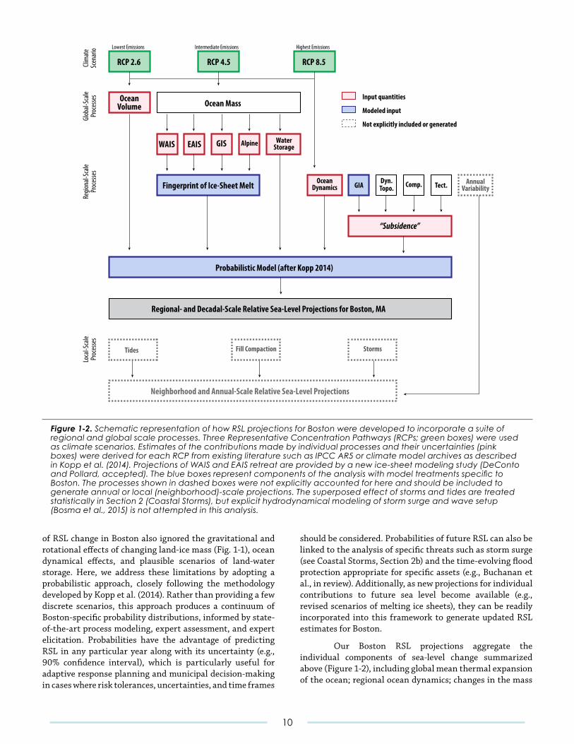
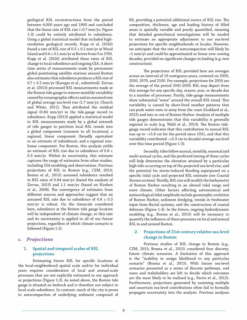
Figure 1-2.SchematicrepresentationofhowRSLprojectionsforBostonweredevelopedtoincorporateasuiteofregionalandglobalscaleprocesses.ThreeRepresentativeConcentrationPathways(RCPs;greenboxes)wereusedasclimatescenarios.Estimatesofthecontributionsmadebyindividualprocessesandtheiruncertainties(pinkboxes)werederivedforeachRCPfromexistingliteraturesuchasIPCCAR5orclimatemodelarchivesasdescribedinKoppetal.(2014).ProjectionsofWAISandEAISretreatareprovidedbyanewice-sheetmodelingstudy(DeContoandPollard,accepted).TheblueboxesrepresentcomponentsoftheanalysiswithmodeltreatmentsspecifictoBoston.Theprocessesshownindashedboxeswerenotexplicitlyaccountedforhereandshouldbeincludedtogenerateannualorlocal(neighborhood)-scaleprojections.ThesuperposedeffectofstormsandtidesaretreatedstatisticallyinSection2(CoastalStorms),butexplicithydrodynamicalmodelingofstormsurgeandwavesetup(Bosmaetal.,2015)isnotattemptedinthisanalysis.

of RSL change in Boston also ignored the gravitational and rotational effects of changing land-ice mass (Fig. 1-1), ocean dynamical effects, and plausible scenarios of land-water storage. Here, we address these limitations by adopting a probabilistic approach, closely following the methodology developed by Kopp et al. (2014). Rather than providing a few discrete scenarios, this approach produces a continuum of Boston-specific probability distributions, informed by state-of-the-art process modeling, expert assessment, and expert elicitation. Probabilities have the advantage of predicting RSL in any particular year along with its uncertainty (e.g., 90% confidence interval), which is particularly useful for adaptive response planning and municipal decision-making in cases where risk tolerances, uncertainties, and time frames

should be considered. Probabilities of future RSL can also be linked to the analysis of specific threats such as storm surge (see Coastal Storms, Section 2b) and the time-evolving flood protection appropriate for specific assets (e.g., Buchanan et al., in review). Additionally, as new projections for individual contributions to future sea level become available (e.g., revised scenarios of melting ice sheets), they can be readily incorporated into this framework to generate updated RSL estimates for Boston.

Our Boston RSL projections aggregate the individual components of sea-level change summarized above (Figure 1-2), including global mean thermal expansion of the ocean; regional ocean dynamics; changes in the mass

WAIS EAIS GIS Alpine

Ocean MassOceanVolume

Fingerprint of Ice-Sheet Melt GIA

“Subsidence”

RCP 2.6 RCP 4.5 RCP 8.5

Lowest Emissions Highest EmissionsIntermediate Emissions

Clim

ate

Scen

ario

Glob

al-Sc

alePr

oces

ses

Regio

nal-S

cale

Proc

esse

s

Dyn.Topo.

OceanDynamics

Probabilistic Model (after Kopp 2014)

Loca

l-Sca

lePr

oces

ses

AnnualVariability

Tides Fill Compaction

Regional- and Decadal-Scale Relative Sea-Level Projections for Boston, MA

Neighborhood and Annual-Scale Relative Sea-Level Projections

Storms

Comp. Tect.

Input quantities

Modeled input

Not explicitly included or generated

WaterStorage

10

of the West Antarctic Ice Sheet (WAIS), East Antarctic Ice Sheet (EAIS), Greenland Ice Sheet (GIS), and alpine glaciers and ice caps (GIC); land-water storage; and the 0.8 ± 0.3 mm/yr of subsidence as described above. As in Kopp et al. (2014), Coupled Model Intercomparison Project Phase 5 (CMIP5) climate models provide projections of thermal expansion and ocean dynamics, and they serve as an input to a model of the mass balance of alpine glaciers and ice caps (GIC); expert elicitation and AR5’s expert assessment provide GIS projections; population projections (United Nations, 2012) and historical data are used for land water storage contributions; and tide-gauge data yield the subsidence rate estimate. Latin hypercube sampling (10,000 samples) is used to generate time-dependent probability distributions of RSL in Boston that consider the cumulative contribution of the individual components and their uncertainties (Kopp et al., 2014). The analysis presented here differs from Kopp et al. (2014), in that projections of future Antarctic Ice Sheet retreat come from a new, physically based modeling study (DeConto and Pollard, 2016) that considers ice-sheet dynamical processes (climate-ice sheet coupling, meltwater-induced hydrofracturing of buttressing ice shelves and structural

collapse of marine-terminating ice cliffs) not considered in previous model studies. These new Antarctic ice sheet simulations, calibrated against past episodes of ice-sheet retreat, show the potential for much greater 21st century Antarctic ice sheet retreat (mostly in West Antarctica) than previously published. This is particularly important for Boston, due to the amplified sensitivity of western North Atlantic sea level to ice loss on West Antarctica (Figure 1-1).

We focus on RCPs 8.5, 4.5, and 2.6. We do not consider RCP6.0, because it yields 21st century sea-level projections nearly identical to those of RCP4.5 (Church et al., 2013). Our projections for GMSL and RSL in Boston under the three RCP scenarios are presented in Figure 1-4 and Table 1-1. Consistent with Kopp et al. (2014), we consider the maximum possible RSL rise to be the 99.9th percentile (equal to an exceedance probability of 0.001 or 0.1%) of our projections. Results are also presented for the median (50th percentile), 67% probability range (16.7th to 83.3th percentiles) and 90% probability range (5th to 95th percentiles). In the terminology used by the IPCC, the 67% and 90% ranges are respectively called “likely” and “very likely.” Due to the influence of regional-scale processes described previously, RSL in Boston will likely exceed the global average throughout the 21st century, regardless of which emissions trajectory is followed.

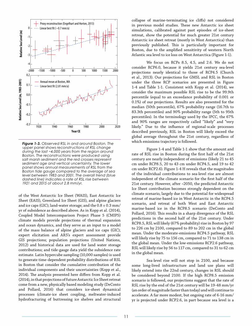
Figure 1-4 and Table 1-1 show that the amount and rate of RSL rise in Boston during the first half of the 21st century are nearly independent of emissions (likely 21 to 45 cm under RCP8.5, 20 to 43 cm under RCP4.5, and 19 to 42 cm under RCP2.6). Figure 1-4 H reveals that the magnitudes of the individual contributions to sea-level rise are almost independent of the climate scenario for the first half of the 21st century. However, after ~2050, the predicted Antarctic Ice Sheet contribution becomes strongly dependent on the climate scenario, largely due to the potential for widespread retreat of marine-based ice in West Antarctic in the RCP4.5 scenario, and retreat of both West and East Antarctic marine-based ice in the RCP8.5 scenario (DeConto and Pollard, 2016). This results in a sharp divergence of the RSL predictions in the second half of the 21st century. Under RCP8.5, RSL will likely (67% probability) rise in Boston by 97 to 226 cm by 2100, compared to 89 to 202 cm in the global mean. Under the moderate-emissions RCP4.5 pathway, RSL will likely rise by 75 to 156 cm, compared to 71 to 138 cm in the global mean. Under the low-emissions RCP2.6 pathway, RSL will likely rise by 56 to 117 cm, compared to 31 to 62 cm in the global mean.

Sea-level rise will not stop in 2100, and because some long-lived infrastructure and land use plans will likely extend into the 22nd century, changes in RSL should be considered beyond 2100. If the high RCP8.5 emission scenario is followed, our projections suggest that the rate of RSL rise by the end of the 21st century will be 19-48 mm/yr (an order of magnitude faster than today) and will continue to accelerate. A far more modest, but ongoing rate of 6-16 mm/yr is projected under RCP2.6, in part because sea level is a

Figure 1-3.ObservedRSLinandaroundBoston.TheupperpanelshowsreconstructionsofRSLchangeduringthelast~4,000yearsfromtheregionaroundBoston.Thereconstructionswereproducedusingsaltmarshsedimentandtheredcrossesrepresentsedimentageandverticaluncertainty.ThelowerpanelshowsannualmeasurementsofRSLfromtheBostontidegaugecomparedtotheaverageofsealevelbetween1983and2001.Theoveralltrend(bluedashedline)indicatesarateofRSLrisebetween1921and2015ofabout2.8mm/yr.

-2000 -1500 -1000 -500 0 500 1000 1500 2000

Rela

tive S

ea Le

vel (

m)

-4

-3

-2

-1

0

Year CE1920 1940 1960 1980 2000 2020

Rela

tive S

ea Le

vel (

m, 1

983-

2001

)

-0.3

-0.2

-0.1

0.0

0.1

0.2

Annual mean at Boston, MALinear best �t (2.81 mm/a)

Proxy reconstruction (Engelhart and Horton, 2013)Linear best �t (~0.7 mm/a)

11

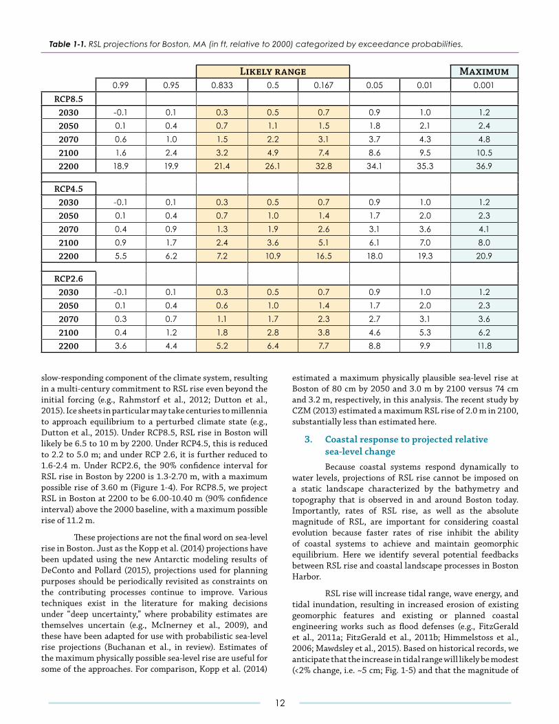
slow-responding component of the climate system, resulting in a multi-century commitment to RSL rise even beyond the initial forcing (e.g., Rahmstorf et al., 2012; Dutton et al., 2015). Ice sheets in particular may take centuries to millennia to approach equilibrium to a perturbed climate state (e.g., Dutton et al., 2015). Under RCP8.5, RSL rise in Boston will likely be 6.5 to 10 m by 2200. Under RCP4.5, this is reduced to 2.2 to 5.0 m; and under RCP 2.6, it is further reduced to 1.6-2.4 m. Under RCP2.6, the 90% confidence interval for RSL rise in Boston by 2200 is 1.3-2.70 m, with a maximum possible rise of 3.60 m (Figure 1-4). For RCP8.5, we project RSL in Boston at 2200 to be 6.00-10.40 m (90% confidence interval) above the 2000 baseline, with a maximum possible rise of 11.2 m.

These projections are not the final word on sea-level rise in Boston. Just as the Kopp et al. (2014) projections have been updated using the new Antarctic modeling results of DeConto and Pollard (2015), projections used for planning purposes should be periodically revisited as constraints on the contributing processes continue to improve. Various techniques exist in the literature for making decisions under “deep uncertainty,” where probability estimates are themselves uncertain (e.g., McInerney et al., 2009), and these have been adapted for use with probabilistic sea-level rise projections (Buchanan et al., in review). Estimates of the maximum physically possible sea-level rise are useful for some of the approaches. For comparison, Kopp et al. (2014)

estimated a maximum physically plausible sea-level rise at Boston of 80 cm by 2050 and 3.0 m by 2100 versus 74 cm and 3.2 m, respectively, in this analysis. The recent study by CZM (2013) estimated a maximum RSL rise of 2.0 m in 2100, substantially less than estimated here.

3. Coastal response to projected relative sea-level change

Because coastal systems respond dynamically to water levels, projections of RSL rise cannot be imposed on a static landscape characterized by the bathymetry and topography that is observed in and around Boston today. Importantly, rates of RSL rise, as well as the absolute magnitude of RSL, are important for considering coastal evolution because faster rates of rise inhibit the ability of coastal systems to achieve and maintain geomorphic equilibrium. Here we identify several potential feedbacks between RSL rise and coastal landscape processes in Boston Harbor.

RSL rise will increase tidal range, wave energy, and tidal inundation, resulting in increased erosion of existing geomorphic features and existing or planned coastal engineering works such as flood defenses (e.g., FitzGerald et al., 2011a; FitzGerald et al., 2011b; Himmelstoss et al., 2006; Mawdsley et al., 2015). Based on historical records, we anticipate that the increase in tidal range will likely be modest (<2% change, i.e. ~5 cm; Fig. 1-5) and that the magnitude of

Likely range   Maximum  0.99 0.95 0.833 0.5 0.167 0.05 0.01 0.001

RCP8.5

2030 -0.1 0.1 0.3 0.5 0.7 0.9 1.0 1.2

2050 0.1 0.4 0.7 1.1 1.5 1.8 2.1 2.4

2070 0.6 1.0 1.5 2.2 3.1 3.7 4.3 4.8

2100 1.6 2.4 3.2 4.9 7.4 8.6 9.5 10.5

2200 18.9 19.9 21.4 26.1 32.8 34.1 35.3 36.9 

RCP4.5

2030 -0.1 0.1 0.3 0.5 0.7 0.9 1.0 1.2

2050 0.1 0.4 0.7 1.0 1.4 1.7 2.0 2.3

2070 0.4 0.9 1.3 1.9 2.6 3.1 3.6 4.1

2100 0.9 1.7 2.4 3.6 5.1 6.1 7.0 8.0

2200 5.5 6.2 7.2 10.9 16.5 18.0 19.3 20.9 

RCP2.6

2030 -0.1 0.1 0.3 0.5 0.7 0.9 1.0 1.2

2050 0.1 0.4 0.6 1.0 1.4 1.7 2.0 2.3

2070 0.3 0.7 1.1 1.7 2.3 2.7 3.1 3.6

2100 0.4 1.2 1.8 2.8 3.8 4.6 5.3 6.2

2200 3.6 4.4 5.2 6.4 7.7 8.8 9.9 11.8

Table 1-1.RSLprojectionsforBoston,MA(inft,relativeto2000)categorizedbyexceedanceprobabilities.

12

2030 2050 2070 2100

0

50

100

150

200

250

2030 2050 2070 2100C D

RCP 2.6RCP 4.5RCP 8.5

67%

90%

99%

1%

RCP 2.6RCP 4.5RCP 8.5

67%

90%

99%

1%

Sea-

Leve

l Rise

(mm

/yr)

0

10

20

30

40

50 RCP 2.6RCP 4.5RCP 8.5

E

1920 1940 1960 1980 2000 2020 2040 2060 2080 2100

1920 1940 1960 1980 2000 2020 2040 2060 2080 2100

Sea L

evel

(cm

, 200

0 CE)

Sea L

evel

(cm

, 200

0 CE)

0

25

50

75

100

125

150 RCP 2.6RCP 4.5RCP 8.5Historic (median with 95% con�dence interval; Hay et al., 2015)

1920 1940 1960 1980 2000 2020 2040 2060 2080 2100

RCP 2.6RCP 4.5RCP 8.5Historic (Boston tide gauge)

B

Global Mean Sea Level Relative Sea Level at Boston, MA

Year CE

2030 2050 2070 2100H

RCP 2

.6RC

P 4.5

RCP 8

.5

Year

2030 2050 2070 21000

25

50

75

100

125

150

Cont

ribut

ion

(cm)

Antarctic Ice SheetGreenland Ice SheetThermal expansionOcean dynamics

Land-water storageGlacio-isostatic adjustment

RCP 2

.6RC

P 4.5

RCP 8

.5

YearAntarctic Ice SheetGreenland Ice SheetThermal expansionGlaciers and ice capsLand-water storage

Year CE

G

Salt-marsh tipping point (~5mm/yr)

Glaciers and ice caps

0

12

24

36

48

60

01224364860728496108

0

12

24

36

48

60

Sea Level (inches, 2000 CE)Sea Level (inches, 2000 CE)

Contribution (inches)

A

0.0

0.5

1.0

1.5

2.0 Sea-Level Rise (inches/yr)

Historic (Hay et al., 2015)

1920 1940 1960 1980 2000 2020 2040 2060 2080 2100

RCP 2.6RCP 4.5RCP 8.5Historic (Boston tide gauge)

F

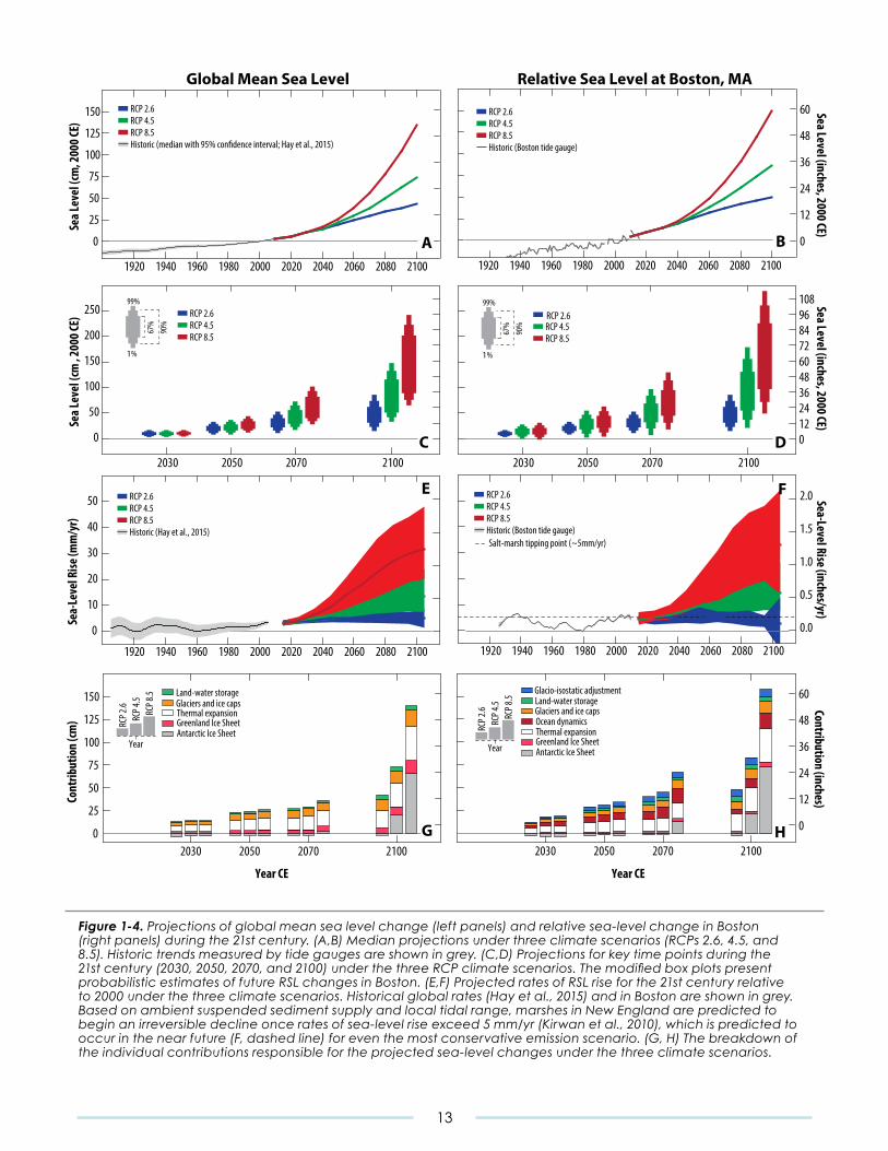
Figure 1-4.Projectionsofglobalmeansealevelchange(leftpanels)andrelativesea-levelchangeinBoston(rightpanels)duringthe21stcentury.(A,B)Medianprojectionsunderthreeclimatescenarios(RCPs2.6,4.5,and8.5).Historictrendsmeasuredbytidegaugesareshowningrey.(C,D)Projectionsforkeytimepointsduringthe21stcentury(2030,2050,2070,and2100)underthethreeRCPclimatescenarios.ThemodifiedboxplotspresentprobabilisticestimatesoffutureRSLchangesinBoston.(E,F)ProjectedratesofRSLriseforthe21stcenturyrelativeto2000underthethreeclimatescenarios.Historicalglobalrates(Hayetal.,2015)andinBostonareshowningrey.Basedonambientsuspendedsedimentsupplyandlocaltidalrange,marshesinNewEnglandarepredictedtobeginanirreversibledeclineonceratesofsea-levelriseexceed5mm/yr(Kirwanetal.,2010),whichispredictedtooccurinthenearfuture(F,dashedline)foreventhemostconservativeemissionscenario.(G,H)Thebreakdownoftheindividualcontributionsresponsiblefortheprojectedsea-levelchangesunderthethreeclimatescenarios.

13

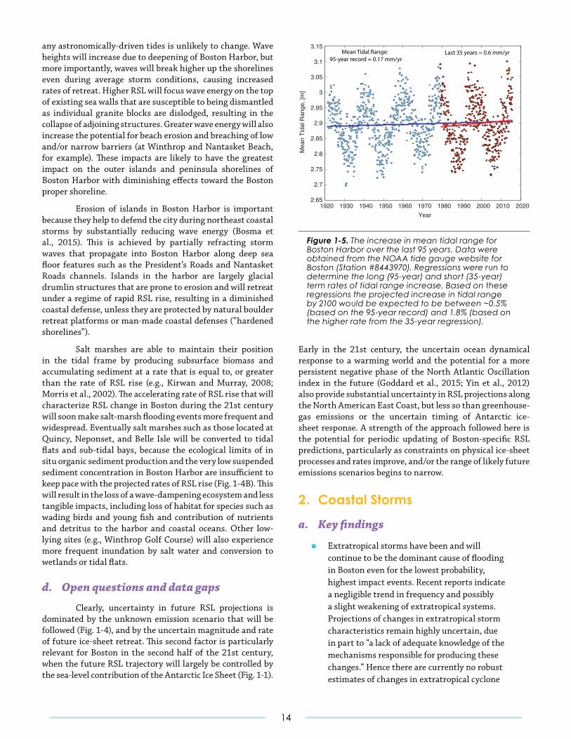
any astronomically-driven tides is unlikely to change. Wave heights will increase due to deepening of Boston Harbor, but more importantly, waves will break higher up the shorelines even during average storm conditions, causing increased rates of retreat. Higher RSL will focus wave energy on the top of existing sea walls that are susceptible to being dismantled as individual granite blocks are dislodged, resulting in the collapse of adjoining structures. Greater wave energy will also increase the potential for beach erosion and breaching of low and/or narrow barriers (at Winthrop and Nantasket Beach, for example). These impacts are likely to have the greatest impact on the outer islands and peninsula shorelines of Boston Harbor with diminishing effects toward the Boston proper shoreline.

Erosion of islands in Boston Harbor is important because they help to defend the city during northeast coastal storms by substantially reducing wave energy (Bosma et al., 2015). This is achieved by partially refracting storm waves that propagate into Boston Harbor along deep sea floor features such as the President’s Roads and Nantasket Roads channels. Islands in the harbor are largely glacial drumlin structures that are prone to erosion and will retreat under a regime of rapid RSL rise, resulting in a diminished coastal defense, unless they are protected by natural boulder retreat platforms or man-made coastal defenses (“hardened shorelines”).

Salt marshes are able to maintain their position in the tidal frame by producing subsurface biomass and accumulating sediment at a rate that is equal to, or greater than the rate of RSL rise (e.g., Kirwan and Murray, 2008; Morris et al., 2002). The accelerating rate of RSL rise that will characterize RSL change in Boston during the 21st century will soon make salt-marsh flooding events more frequent and widespread. Eventually salt marshes such as those located at Quincy, Neponset, and Belle Isle will be converted to tidal flats and sub-tidal bays, because the ecological limits of in situ organic sediment production and the very low suspended sediment concentration in Boston Harbor are insufficient to keep pace with the projected rates of RSL rise (Fig. 1-4B). This will result in the loss of a wave-dampening ecosystem and less tangible impacts, including loss of habitat for species such as wading birds and young fish and contribution of nutrients and detritus to the harbor and coastal oceans. Other low-lying sites (e.g., Winthrop Golf Course) will also experience more frequent inundation by salt water and conversion to wetlands or tidal flats.

d. Open questions and data gaps

Clearly, uncertainty in future RSL projections is dominated by the unknown emission scenario that will be followed (Fig. 1-4), and by the uncertain magnitude and rate of future ice-sheet retreat. This second factor is particularly relevant for Boston in the second half of the 21st century, when the future RSL trajectory will largely be controlled by the sea-level contribution of the Antarctic Ice Sheet (Fig. 1-1).

Early in the 21st century, the uncertain ocean dynamical response to a warming world and the potential for a more persistent negative phase of the North Atlantic Oscillation index in the future (Goddard et al., 2015; Yin et al., 2012) also provide substantial uncertainty in RSL projections along the North American East Coast, but less so than greenhouse-gas emissions or the uncertain timing of Antarctic ice-sheet response. A strength of the approach followed here is the potential for periodic updating of Boston-specific RSL predictions, particularly as constraints on physical ice-sheet processes and rates improve, and/or the range of likely future emissions scenarios begins to narrow.

2. Coastal Storms

a. Key findings

■ Extratropical storms have been and will continue to be the dominant cause of flooding in Boston even for the lowest probability, highest impact events. Recent reports indicate a negligible trend in frequency and possibly a slight weakening of extratropical systems. Projections of changes in extratropical storm characteristics remain highly uncertain, due in part to “a lack of adequate knowledge of the mechanisms responsible for producing these changes.” Hence there are currently no robust estimates of changes in extratropical cyclone

Figure 1-5.TheincreaseinmeantidalrangeforBostonHarboroverthelast95years.DatawereobtainedfromtheNOAAtidegaugewebsiteforBoston(Station#8443970).Regressionswereruntodeterminethelong(95-year)andshort(35-year)termratesoftidalrangeincrease.Basedontheseregressionstheprojectedincreaseintidalrangeby2100wouldbeexpectedtobebetween~0.5%(basedonthe95-yearrecord)and1.8%(basedonthehigherratefromthe35-yearregression).

1920 1930 1940 1950 1960 1970 1980 1990 2000 2010 2020Year

Mean Tidal Range: 95-year record = 0.17 mm/yr

Last 35 years = 0.6 mm/yr

2.7

2.75

2.8

2.85

2.9

2.95

3

3.05

3.1

3.15

Mea

n Ti

dal R

ange

, [m

]

2.65

14

intensity, frequency, or trajectory for any of the time periods under consideration here.

■ There is still disagreement with respect to changes in tropical cyclone frequency; however, there is agreement that tropical storm intensity is likely to increase, resulting in an increase in the frequency of major hurricanes (Category 3 and greater) and an increase in the intensities of the strongest storms. Combined with a projected northward shift in both the track and intensity of these storms, the impact of tropical cyclones upon Boston has the potential to increase even if the total number of storms does not. Some projections for increased exceedance probabilities of hurricane-induced surge activity have been produced, albeit not for specific times/scenarios and not with accompanying uncertainties (see Fig. 4.24, Bosma et al., 2015). Other than these estimates, to the best of our knowledge, no changes in intensity, frequency, or tracks have been produced for New England. Given the uncertainty in the response of these storms to changing environmental conditions associated with global warming, currently there are no robust estimates of changes in tropical cyclone intensity, frequency, or trajectory for any of the time periods under consideration here.

■ Given the uncertainties in changes in tropical and extratropical storms, we recommend that no changes be assumed in characteristics but this be further monitored as this is a rapidly evolving branch of climate science.

■ Moving forward, independent of changes in coastal storms, the most substantial influence of global warming upon storm-induced flooding will be the increase in global and local sea levels, which will increase the baseline water level upon which the storm surge and storm tide are superimposed.

■ Coastal flooding study results indicate modest increases in flooding frequency and magnitude by 2030 under most emissions scenarios and more substantial increases in storm-induced flooding by 2050 and later. For instance, coastal floods that presently occur with a 1% annual likelihood (i.e., a “100-year storm tide”) in 2000 could have a higher than 20% annual likelihood of occurring by the year 2050 and may occur as frequently as high tide sometime near or after year 2100.

■ To date, coastal flooding studies have used fixed

sea level rise elevations at points in the future, rather than probabilistic estimates such as those shown in Table 1-1. Differences are not expected to dramatically affect the estimates of the heights and recurrence rates of particular water surface elevations through 2050 compared to 2000; however, the same does not hold true for later in the century. Indeed, results suggest that incorporating fixed median SLR estimates for 2100, rather than accounting for the full distribution, halves the height of the expected 1% annual probability flood and underestimates it by over 1 m.

b. Review of existing science

1. Definitions Storms—infrequent but severe weather events that are typically accompanied by high winds, heavy precipitation, and dramatic changes in temperature—can strike Boston at any time of the year. While there are various types of atmospheric conditions that can produce storms across the region, our primary interest here is in the large-scale (100s of miles) counterclockwise circulations that spiral around traveling low-pressure centers, termed “cyclones.” These circulations, and the accompanying increase in near-surface winds, can damage structures across the city, produce flying debris that can cause injury and even death in certain cases, and disrupt electricity and communications services. Even more substantial damages result when winds from storms centered off the coast drive ocean water towards the land, resulting in a local rise in the water level, termed the “storm surge.” When combined with tidal influences, the wind-driven increase in sea-level is known as the “storm tide” (NHCRHC, 2014) and can result in storm-induced flooding across the city.

Traveling cyclones can originate from various dynamic processes. In the tropics, the low pressures at the center of the cyclone are the result of feedbacks between the atmosphere and ocean. In-spiraling near-surface winds draw moisture from the ocean and feed it into the cyclone, which through circulating updrafts lofts the moisture, allowing it to condense. As it does so, it releases heat that warms the surrounding air, causing it to rise even more rapidly. As the air rises, the atmospheric pressures below it decrease even further, which subsequently draws even more warm, moist air into the cyclone. These storms, termed “tropical cyclones,” are referred to as hurricanes (in the North American sector) once they have reached a sustained wind speed of more than 74mph. For this report, however, we will use the term “tropical cyclone” to refer to any sustained storm system originating from the tropics that subsequently impacts the Northeast.

Traveling cyclones can also originate from outside

15

the tropics, which are termed “extratropical cyclones.” For these storms the low pressure at the center of the cyclone typically results from atmospheric processes that rely on the difference in temperatures between the low and high latitudes, which serves as a source of “potential energy” that can drive the kinetic energy of the storm itself. In this case, the circulation of air around the storm’s low (and high) pressure center pushes warm, moist low-latitude air into regions of the storm that are already warm and draws cold, dry high-latitude air into regions of the storm that are already cold. The movement of these air masses augments the pressure difference between the low and high pressure centers of the storm, resulting in stronger winds and even more infusion of warm and cold air into the storm. These storms—which can form during any time of year but are most prevalent in the extended cold-season months—include nor’easters as well as “coastal runners” and “Alberta Clippers” among others. For this report, however, we will use the term “extratropical cyclone” to refer to any sustained storm system originating from the mid-latitudes that subsequently impacts the Northeast.

2. Tropical Cyclones Nationwide, hurricane losses have been on the rise during the 20th century, partly as a result of an increase in intensity and duration of Atlantic hurricanes. However, trends in the frequency and/or intensity of tropical cyclones within any given region, including the Northeast, are much less robust (NHCRHC, 2014; Bosma et al., 2015). Indeed, the Intergovernmental Panel on Climate Change assessment (IPCC, 2013) suggests the frequency of Atlantic tropical storms is unlikely to increase over the next century, although alternate projections using different models and downscaling techniques do suggest a possible increase in frequency (Emanuel, 2013). Despite this discrepancy in the projection of tropical cyclone frequency, there is agreement on the projection of tropical storm intensity, which is likely to increase, resulting in an increase in the frequency of major hurricanes (Category 3+ - NHCRHC, 2014). Combined with a projected northward shift in both the track and intensity of these storms, the impact of tropical cyclones upon Boston has the potential to increase even if the total number of storms does not (NHCRHC, 2014).

Some projections for increased exceedance probabilities of hurricane-induced surge activity have been produced, albeit not for specific times/scenarios and not with accompanying uncertainties (Fig. 4.24, Bosma et al., 2015). Other than these estimates, to the best of our knowledge, no changes in intensity, frequency, or tracks have been produced for New England.

3. Extratropical Cyclones While early reports suggested that extratropical storm tracks, including those of nor’easters, have shifted northward since the 1970s resulting in more frequent and intense storm activity in New England (NECIA, 2007), more recent reports indicate a negligible trend in frequency and

possibly a slight weakening of these systems (NHCRHC, 2014; Bosma et al., 2015). Given these discrepancies, no definitive trend in the frequency and/or intensity of extratropical storms over New England has yet been reported (NHCRHC, 2014). In addition, few numerical model studies have been done on the changing impacts of extratropical storms on coastal areas of the Northeast (Bosma et al., 2015). Of those that have been done, most conclude that a warmer climate and accompanying decrease in the temperature difference between low and high latitudes results in a small poleward shift of the storm tracks, a reduction in their number as well as possibly their intensity (Bosma et al., 2015). More locally, it is expected that there will be a decrease in the frequency of high-intensity storms off the coast of the Northeast (Colle et al., 2013; Seiler and Zweirs, 2015) while inland there is the potential for more high-intensity storms (Colle et al., 2013). However, alternate projections using different models suggest a possible decrease inland as well (Seiler and Zweirs, 2015). In addition, these effects may be seasonally dependent with some projections suggesting 5 to 15 percent more late-winter storms affecting the Northeast (about one additional late winter storm per year) under very large climate change scenarios (NECIA, 2007; MassCCAR, 2011).

As with projections of changes in tropical cyclone characteristics, no projections of changes in extratropical cyclone intensity, frequency, or tracks have been produced for the Northeast. One study (Colle et al., 2013) does produce projections for changes in intensity and frequency along the East Coast of the U.S., including a decrease in the frequency of weak to moderate cyclones both over land and off-shore. The same study indicates an increase in the frequency of intense storms over land (but no discernable change in frequency of intense storms off-shore), although a more recent study (using different models) indicates these same regions will instead experience a substantial decrease (of 15-20%) in exposure to “explosive cyclones” (Seller and Zwiers, 2015).

4. Storm-Induced Coastal Flooding As noted above, Boston is sensitive to coastal flooding resulting from both tropical and extratropical storms. The actual size of the storm-induced surge depends upon the storm’s intensity, speed, size, and track with respect to the coast (NHCRHC, 2014). Just as important is the timing of a storm in relation to the tide, particularly in Boston where the tidal ranges (~3-4 m) are typically larger than the storm surge itself and hence contribute relatively more to the overall storm tide than in a place such as New York City where the tidal range is half that in Boston (Bosma et al., 2015). Since tropical cyclones almost always make landfall south of Boston and move through the region relatively quickly, there is a substantially smaller chance that the accompanying storm surge will coincide with high tide. In contrast, the storm surges induced by extratropical storms often last a day or more. For this reason, currently extratropical storms are the dominant form of flooding in Boston even for the lowest probability, highest impact events

16

(Bosma et al., 2015). Moving forward, the most substantial influence of global warming upon storm-induced flooding will be the increase in global and local sea levels, which will increase the baseline water level upon which the storm surge and storm tide are superimposed. Obviously, storm-induced flooding could also be impacted by changes in extratropical and tropical storm frequencies and intensities (NHCRHC, 2014), however as noted previously the nature of these changes are much less certain. Even absent changes in the characteristics of these storms, global and local sea level rise alone will expose infrastructure to storm-induced flooding such that the projected 100-year coastal storm floodplain in 2100 will include much of the Back Bay and Boston waterfront areas, including Logan International Airport, the Deer Island Sewage Treatment Plant, and the Central Artery and Massachusetts Turnpike (MassCCAR, 2011).

c. Projections

Given the uncertainties in the changing characteristics of tropical and extratropical storms, many early studies used the present frequency distributions for storm tides measured at tide gauges, elevated by sea level rise projections, and then mapped the hydraulically connected areas with the same elevation as at the gauge (so-called “bathtub” studies). More recent studies, though, tend to use various hydraulic models to estimate the response of the coastal ocean to storm-induced winds (Bosma et al., 2015). Generally, these latter results indicate that flooding frequency and magnitude increases by 2030 under most emissions scenarios, but these changes are moderate compared to more substantial increases in storm-induced flooding by 2050 and later (Bosma et al., 2015). For instance, coastal floods that presently occur with a 1% annual likelihood (i.e., a “100-year storm tide”) in 2005 could have a higher than 20% annual likelihood of occurring by the year 2050 and may occur as frequently as high tide sometime near or after year 2100 (Kirshen et al., 2008; TBHA, 2013). Geographically, 2070 projections using a 98cm rise in sea level relative to 2013 indicate the annual likelihood of flooding for the financial district, waterfront and in South and East Boston exceed 50% and are as high as 1% for Logan Airport (Bosma et al., 2015).

Unfortunately, given the computational resources needed to simulate the storm surge and tide using hydraulic models, these more recent studies use fixed estimates of sea level rise that ignore the probabilistic projections of sea level rise that may impact Boston (Bosma et al., 2015); by extension they are incapable of fully representing the full distribution of changes in storm-induced flooding that may occur at various time periods and under various scenarios. While differences in the use of the fixed and probabilistic distributions of sea level rise are not expected to dramatically affect the estimates of return levels and recurrence rates of particular water surface elevations up through 2050 (when the distributions of sea level rise are relatively narrow), the same does not hold for later in the century. Indeed, results

suggest that incorporating fixed median SLR estimates for 2000 to 2100, rather than accounting for the full distribution, halves the height of the expected 1% annual probability flood and underestimates it by over 1m (Buchanan et al., 2016).

As such, for this report, we return to the use of the historic  frequency distributions for storm tides, as represented by tide gauge-derived extreme value statistics used in Buchanan et al. (2016). These annual chance flood events  are then increased by the distributions of sea level rise (SLR) as given in the SLR Section of this report using the methods outlined in Hunter (2012) and Buchanan et al. (2016). Developed by Hunter (2012) and expanded by Buchanan et al. (2016), SLR  “allowances” provide planners with a  “freeboard” (vertical distance to raise a structure) to maintain a desired annual flooding exposure (e.g., 1% average annual chance of flooding) for either a specific future year (instantaneous allowance) or over a given time period (design-life allowance) with SLR. Importantly, because the number of exceedances is a nonlinear function of the flood level (whether calculated using a theoretical distribution such as Gumbel distribution, an empirical distribution such as the peak-over-threshold approach as done here, or from the observations themselves)  and  the flood level is a function of both the storm tide and SLR, the uncertainty in SLR estimates introduces a positive definite increase in the expected number of exceedances above that estimated using the mean (or median) SLR value – see Eq.7 from Hunter (2012). For example, the extent of uncertainty in a SLR probability distribution and  the log-linearity of the flood return curve pulls the height of the expected 1% average annual chance flood towards the 99.9th percentile of SLR. Essentially, the number of additional exceedances introduced by the possibility of larger than expected SLR is not offset by the reduction of exceedances introduced by the possibility of smaller than expected SLR, even if the SLR distribution itself is near-normal. Because of this non-linear effect, the allowance needed to maintain exposure to flooding events given a distribution of SLR values is larger than would be estimated using the mean (or median) value of that SLR distribution, as discussed above and quantified in Buchanan et al. (2016). The results of this analysis are in Table 2-1.

In the near- (2030) and mid-term (2050), both the annual probability of today’s 100-year flood and the heights for a 1% probability flood are relatively insensitive to the concentration pathway/emissions scenario. However, by the end of the century (and even before) the differences between the values under the high (RCP8.5) and low (RCP4.5) concentration conditions become substantial. Further, the magnitudes of these values, in comparison to current ones, are also substantial. For instance, under both scenarios the probability of the current (circa 2000) 100-year flood becomes sub-annual and may occur as frequently as daily given the distributions of expected sea level rise. Further, under both scenarios the heights for a 1% probability flood are ~1.5-2.5m higher than today, the latter value representing a near doubling of their current value.

17

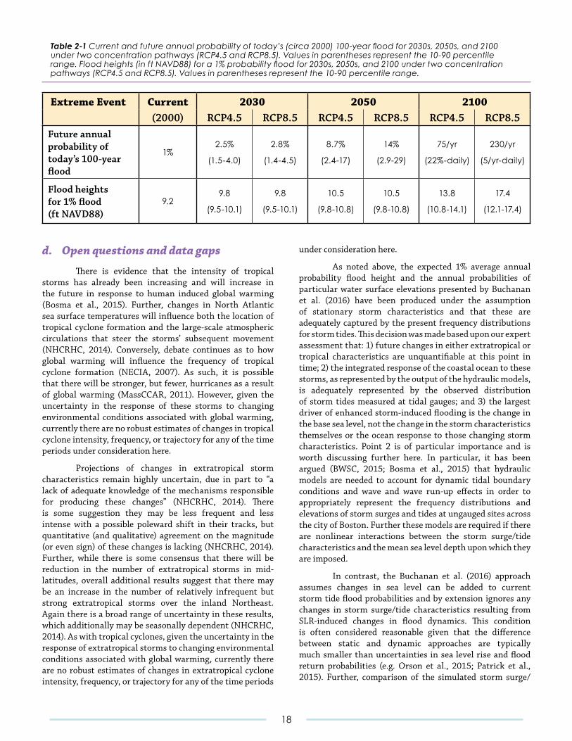
d. Open questions and data gaps

There is evidence that the intensity of tropical storms has already been increasing and will increase in the future in response to human induced global warming (Bosma et al., 2015). Further, changes in North Atlantic sea surface temperatures will influence both the location of tropical cyclone formation and the large-scale atmospheric circulations that steer the storms’ subsequent movement (NHCRHC, 2014). Conversely, debate continues as to how global warming will influence the frequency of tropical cyclone formation (NECIA, 2007). As such, it is possible that there will be stronger, but fewer, hurricanes as a result of global warming (MassCCAR, 2011). However, given the uncertainty in the response of these storms to changing environmental conditions associated with global warming, currently there are no robust estimates of changes in tropical cyclone intensity, frequency, or trajectory for any of the time periods under consideration here.

Projections of changes in extratropical storm characteristics remain highly uncertain, due in part to “a lack of adequate knowledge of the mechanisms responsible for producing these changes” (NHCRHC, 2014). There is some suggestion they may be less frequent and less intense with a possible poleward shift in their tracks, but quantitative (and qualitative) agreement on the magnitude (or even sign) of these changes is lacking (NHCRHC, 2014). Further, while there is some consensus that there will be reduction in the number of extratropical storms in mid-latitudes, overall additional results suggest that there may be an increase in the number of relatively infrequent but strong extratropical storms over the inland Northeast. Again there is a broad range of uncertainty in these results, which additionally may be seasonally dependent (NHCRHC, 2014). As with tropical cyclones, given the uncertainty in the response of extratropical storms to changing environmental conditions associated with global warming, currently there are no robust estimates of changes in extratropical cyclone intensity, frequency, or trajectory for any of the time periods

under consideration here.

As noted above, the expected 1% average annual probability flood height and the annual probabilities of particular water surface elevations presented by Buchanan et al. (2016) have been produced under the assumption of stationary storm characteristics and that these are adequately captured by the present frequency distributions for storm tides. This decision was made based upon our expert assessment that: 1) future changes in either extratropical or tropical characteristics are unquantifiable at this point in time; 2) the integrated response of the coastal ocean to these storms, as represented by the output of the hydraulic models, is adequately represented by the observed distribution of storm tides measured at tidal gauges; and 3) the largest driver of enhanced storm-induced flooding is the change in the base sea level, not the change in the storm characteristics themselves or the ocean response to those changing storm characteristics. Point 2 is of particular importance and is worth discussing further here. In particular, it has been argued (BWSC, 2015; Bosma et al., 2015) that hydraulic models are needed to account for dynamic tidal boundary conditions and wave and wave run-up effects in order to appropriately represent the frequency distributions and elevations of storm surges and tides at ungauged sites across the city of Boston. Further these models are required if there are nonlinear interactions between the storm surge/tide characteristics and the mean sea level depth upon which they are imposed.

In contrast, the Buchanan et al. (2016) approach assumes changes in sea level can be added to current storm tide flood probabilities and by extension ignores any changes in storm surge/tide characteristics resulting from SLR-induced changes in flood dynamics. This condition is often considered reasonable given that the difference between static and dynamic approaches are typically much smaller than uncertainties in sea level rise and flood return probabilities (e.g. Orson et al., 2015; Patrick et al., 2015). Further, comparison of the simulated storm surge/

Extreme Event Current 2030 2050 2100 (2000)  RCP4.5 RCP8.5 RCP4.5 RCP8.5 RCP4.5 RCP8.5Future annual probability of today’s 100-year flood

1%2.5%

(1.5-4.0)

2.8%

(1.4-4.5)

8.7%

(2.4-17)

14%

(2.9-29)

75/yr

(22%-daily)

230/yr

(5/yr-daily)

Flood heights for 1% flood (ft NAVD88)

9.29.8

(9.5-10.1)

9.8

(9.5-10.1)

10.5

(9.8-10.8)

10.5

(9.8-10.8)

13.8

(10.8-14.1)

17.4

(12.1-17.4)

Table 2-1Currentandfutureannualprobabilityoftoday’s(circa2000)100-yearfloodfor2030s,2050s,and2100undertwoconcentrationpathways(RCP4.5andRCP8.5).Valuesinparenthesesrepresentthe10-90percentilerange.Floodheights(inftNAVD88)fora1%probabilityfloodfor2030s,2050s,and2100undertwoconcentrationpathways(RCP4.5andRCP8.5).Valuesinparenthesesrepresentthe10-90percentilerange.

18

tide characteristics for different SLR estimates, as derived in Bosma et al., 2015, indicate that the influence of these nonlinear interactions are minimal such that the simulated storm surge/tide characteristics remain relatively stationary as a function of SLR and that these characteristics are well represented by the observed characteristics at gauged sites.

These findings have two important implications. Firstly, they suggest that for Boston (although not for all coastal locations) the historical storm surge/tide characteristics from gauged stations can be used as a proxy for future storm surge/tide characteristics, which in turn allows us to provide quantitative projections of flood elevations consistent with the distributions of sea level rise as given in the SLR Section (as presented in Table 1-1). Equally important, they provide guidance on how to synthesize data from hydraulic models with the improved distributions of sea level rise found in the SLR Section, which is essential for projecting the expected flood height for various return levels, scenarios and time periods at ungauged sites across Boston. Specifically, using the data at a particular hydraulic model grid, the necessary extreme value statistics can be derived from the frequency distributions and elevations of storm surges and tides at that grid using the methods outlined in Buchanan et al. (2016). These extreme value statistics then can be increased by the distributions of sea level rise as given in the SLR Section, again as outlined in Buchanan et al. (2016). While not done here, in this way improved projections of expected flood heights for various return levels, scenarios and time periods for any location in the city can be determined using the frequency distributions of storm surges/tides provided by the hydraulic model. As such, we strongly advise that subsequent vulnerability analyses adopt this method.

As an aside, we further note that while results presented here are for the historic and future 100-year flood level/probability—which is a standard for risk management—alternative dynamic flood risk analyses are available that allow decision-makers to assess investments across time lines, risk tolerance levels, and confidence in sea-level rise projections (vis Buchanan et al., 2016). As such, we further advise that future vulnerability analyses adopt these methods in the face of a changing and uncertain distribution across all flood return periods.

e. Joint flooding between rain- and storm surge-driven flooding

Floods at a given location can be caused by one or more coinciding events (e.g., riverine flooding, tidal surges, snowmelt runoff, and urban drainage). However, traditional flood frequency analysis does not often distinguish the multiple factors that generate floods but instead analyzes flood peaks as single, independent events. Such analysis, while computationally convenient, can be hydrodynamically incorrect, and can lead to erroneous estimates of flood magnitude and risk (Bray and McCuen, 2014). For coastal

communities such as Boston, the flood factor of greatest interest (and concern) is the probability of coincidence (or joint probability) of extreme rain-driven and extreme storm surge-driven floods. Vogel and Stedinger (1984) and Stedinger et al. (1993) recommended a composite flood probability distribution method for independent flood generating processes, which was used in Bosma et al. (2015) to develop the flood exceedance probabilities generated by both tropical and extratropical storms. Recent studies have assessed the joint probabilities of rain- and storm surge-driven flooding using hydrodynamic modeling (van den Hurk et al., 2015; Bosma et al., 2015), copula-based models (Xu et al., 2014; Wahl et al., 2015) or other statistical methods (Lamb et al., 2010; Irish and Resio, 2013; Zheng et al., 2014). In particular, Wahl et al. (2015) evaluated the correlation between extreme rainfall and storm surge events along the US coastline for two cases: Case I, the highest annual storm surge correlated with the highest rainfall within ±1 day and Case II, the highest annual rainfall event correlated with the highest surge event within ±1 day. In Boston, they report a fairly low Kendall’s τ correlation (τ ~ 0.2) for Case I and no correlation for Case II. They also evaluated how this correlation changed over the period of record. In the case of Boston, the Case I correlation was very low (~0.1) and statistically insignificant until around 1965 (see Fig. 2f of Wahl et al., 2015). Between 1965 and around 1990, the correlation increased (but still fairly low, τ ~ 0.2) and became statistically significant. After 1990, the correlation increased from ~0.2 to ~0.3. Increasing trends in extreme rainfall have been reported for the time period from 1970 onwards (e.g. Douglas and Fairbank, 2011) and increased rates of global sea level rise have been reported after 1990 (Holgate and Woodworth, 2004).

Figure 2-1 shows the results of preliminary, as yet unpublished analysis of the temporal coincidence of daily rainfall measured at Logan International Airport with maximum daily water level anomalies (WLA, observed water level minus predicted tide, representing storm surge following Kirshen et al., 2008, Fig. 2-1a) and daily observed total water levels (TWL, tide plus surge; Fig. 2-1b) measured in Boston Harbor on the same day. The blue X symbols represent the entire record (1921 to present) while the red squares represent events since 1990. Fig. 2-1a supports the findings of Wahl et al. (2015) that there is a relatively low coincidence of extreme rainfall with extreme surge events on the same day (±1 day coincidence was not evaluated). Figure 2-1b shows that the highest rainfall events have generally coincided with TWL of 2500 and 3000 mm, within the middle to upper levels of TWL observed in Boston Harbor. Plotting the observations since 1990 shows that the distribution of WLA coinciding with rainfall does not appear to have shifted over time (as was suggested by Wahl et al., 2015), however, there does appear to have been a slight increase in the magnitude of TWL coinciding with daily precipitation.

The New Charles River Dam and the Amelia Earhart Dam (on the lower Mystic) were constructed to block the upstream migration of the tide and essentially transformed the lower Charles and Mystic estuaries into freshwater basins

19

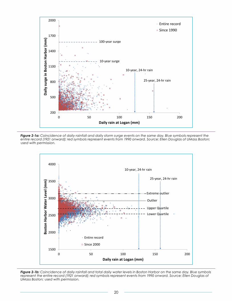
200

500

800

1100

1400

1700

2000

0 50 100 150 200

Dai

ly su

rge

in B

osto

n H

arbo

r (m

m)

Daily rain at Logan (mm)

Entire recordSince 1990

100-year surge

10-year surge

10-year, 24-hr rain

25-year, 24-hr rain

1500

2000

2500

3000

3500

4000

0 50 100 150 200

Bost

on H

arbo

r Wat

er L

evel

(mm

)

Daily rain at Logan (mm)

Entire record

Since 2000

Lower Quartile

Upper Quartile

Outlier

Extreme outlier

10-year, 24-hr rain

25-year, 24-hr rain

Figure 2-1a: Coincidenceofdailyrainfallanddailystormsurgeeventsonthesameday.Bluesymbolsrepresenttheentirerecord(1921onward);redsymbolsrepresenteventsfrom1990onward.Source:EllenDouglasofUMassBoston;usedwithpermission.

Figure 2-1b: CoincidenceofdailyrainfallandtotaldailywaterlevelsinBostonHarboronthesameday.Bluesymbolsrepresenttheentirerecord(1921onward);redsymbolsrepresenteventsfrom1990onward.Source:EllenDouglasofUMassBoston;usedwithpermission.

20

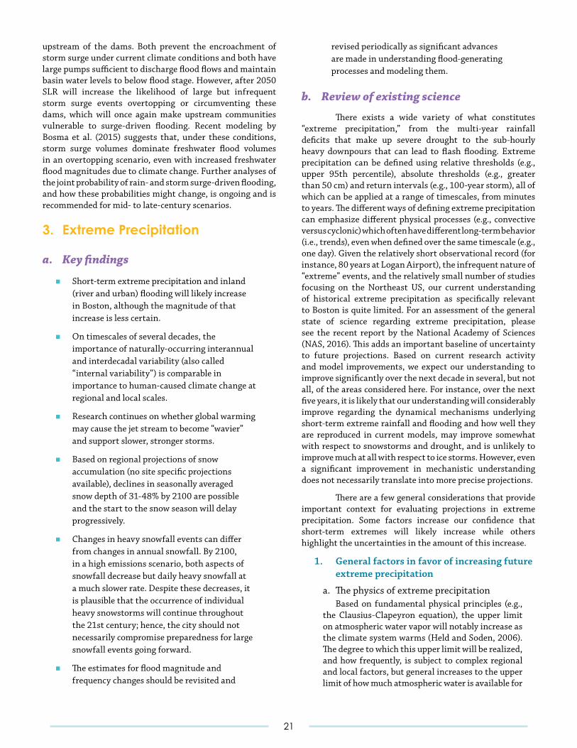
upstream of the dams. Both prevent the encroachment of storm surge under current climate conditions and both have large pumps sufficient to discharge flood flows and maintain basin water levels to below flood stage. However, after 2050 SLR will increase the likelihood of large but infrequent storm surge events overtopping or circumventing these dams, which will once again make upstream communities vulnerable to surge-driven flooding. Recent modeling by Bosma et al. (2015) suggests that, under these conditions, storm surge volumes dominate freshwater flood volumes in an overtopping scenario, even with increased freshwater flood magnitudes due to climate change. Further analyses of the joint probability of rain- and storm surge-driven flooding, and how these probabilities might change, is ongoing and is recommended for mid- to late-century scenarios.

3. Extreme Precipitation

a. Key findings

■ Short-term extreme precipitation and inland (river and urban) flooding will likely increase in Boston, although the magnitude of that increase is less certain.

■ On timescales of several decades, the importance of naturally-occurring interannual and interdecadal variability (also called “internal variability”) is comparable in importance to human-caused climate change at regional and local scales.

■ Research continues on whether global warming may cause the jet stream to become “wavier” and support slower, stronger storms.

■ Based on regional projections of snow accumulation (no site specific projections available), declines in seasonally averaged snow depth of 31-48% by 2100 are possible and the start to the snow season will delay progressively.

■ Changes in heavy snowfall events can differ from changes in annual snowfall. By 2100, in a high emissions scenario, both aspects of snowfall decrease but daily heavy snowfall at a much slower rate. Despite these decreases, it is plausible that the occurrence of individual heavy snowstorms will continue throughout the 21st century; hence, the city should not necessarily compromise preparedness for large snowfall events going forward.

■ The estimates for flood magnitude and frequency changes should be revisited and

revised periodically as significant advances are made in understanding flood-generating processes and modeling them.

b. Review of existing science

There exists a wide variety of what constitutes “extreme precipitation,” from the multi-year rainfall deficits that make up severe drought to the sub-hourly heavy downpours that can lead to flash flooding. Extreme precipitation can be defined using relative thresholds (e.g., upper 95th percentile), absolute thresholds (e.g., greater than 50 cm) and return intervals (e.g., 100-year storm), all of which can be applied at a range of timescales, from minutes to years. The different ways of defining extreme precipitation can emphasize different physical processes (e.g., convective versus cyclonic) which often have different long-term behavior (i.e., trends), even when defined over the same timescale (e.g., one day). Given the relatively short observational record (for instance, 80 years at Logan Airport), the infrequent nature of “extreme” events, and the relatively small number of studies focusing on the Northeast US, our current understanding of historical extreme precipitation as specifically relevant to Boston is quite limited. For an assessment of the general state of science regarding extreme precipitation, please see the recent report by the National Academy of Sciences (NAS, 2016). This adds an important baseline of uncertainty to future projections. Based on current research activity and model improvements, we expect our understanding to improve significantly over the next decade in several, but not all, of the areas considered here. For instance, over the next five years, it is likely that our understanding will considerably improve regarding the dynamical mechanisms underlying short-term extreme rainfall and flooding and how well they are reproduced in current models, may improve somewhat with respect to snowstorms and drought, and is unlikely to improve much at all with respect to ice storms. However, even a significant improvement in mechanistic understanding does not necessarily translate into more precise projections.

There are a few general considerations that provide important context for evaluating projections in extreme precipitation. Some factors increase our confidence that short-term extremes will likely increase while others highlight the uncertainties in the amount of this increase.

1. General factors in favor of increasing future extreme precipitation

a. The physics of extreme precipitation Based on fundamental physical principles (e.g., the Clausius-Clapeyron equation), the upper limit on atmospheric water vapor will notably increase as the climate system warms (Held and Soden, 2006). The degree to which this upper limit will be realized, and how frequently, is subject to complex regional and local factors, but general increases to the upper limit of how much atmospheric water is available for

21

precipitation (and for fueling storms via latent heat release) will occur as the climate warms.

b. Model-to-model consistency While regional projections of precipitation extremes vary considerably based on model and scenario (Ning et al., 2015, Vavrus et al., 2015), all individual results show increases (Ning et al. 2015). Model-to-model consistency in the direction of change is a strong factor in assigning confidence to projections, which increases our confidence that extreme precipitation will generally increase. However, the variability in individual model results reduces our confidence in the magnitude of the increase. Furthermore, model consistency is not a guarantee of an accurate result – there are known limitations common to all current models that are directly relevant to extreme precipitation, including insufficient resolution to explicitly resolve hurricanes as well as individual convective storm cells.

c. Observed trends The Northeast has already exhibited notable increases in extreme precipitation. For example, the Northeast US has experienced a greater than 70% increase in the heaviest 1% of daily precipitation over the period 1958-2010, which represents the highest regional increase in the US (Groisman et al., 2012, Kunkel et al., 2013a, Walsh et al., 2014). The Northeast has also experienced a documented increase in flooding (Collins, 2009, DeGaetano, 2009, Armstrong et al., 2014, Peterson et al., 2013, Georgakakos et al., 2014). While the existence of trends in historical observations does not guarantee trends in future events, the prominence of the extreme precipitation trend, especially in combination with the consistency in the sign of model projections for extreme precipitation, is highly suggestive of future increases, and sets a minimum level of what is physically possible.

2. General factors that increase the uncertainty of the projections

a. Hurricanes Hurricanes, hurricane remnants, and tropical cyclones (the same type of storm system as a hurricane but weaker) are important mechanisms for the occurrence of the highest precipitation events in the Northeast (Barlow, 2012) and some of the most severe floods (e.g., the impact of coastal flooding of Hurricane Sandy in NYC or the inland flooding associated with Hurricanes Connie and Diane; see also Collins et al., 2014). Shifts in the intensity, frequency, or paths of these systems could have important implications for extreme precipitation and flooding but these systems are not fully resolved in current climate models. This is

discussed in more detail in the previous section on storms.

b. Naturally-occurring climate variability On timescales of several decades, the importance of naturally-occurring interannual and interdecadal variability (also called “internal variability”) is comparable in importance to human-caused climate change at regional and local scales. To discriminate between the two, a large number of model runs (Deser et al., 2012, 2014; Wallace et al., 2014) or special techniques (Thompson et al., 2015) is required. Indeed, ongoing research continues to refine the extent to which natural variability (i.e., long-term persistence) influences the historical trends.

c. Model differences and limited evaluation of simulated extremes

As noted previously, regional projections of precipitation extremes vary considerably based on model and scenario (Ning et al., 2015, Vavrus et al., 2015). One factor in the credibility of a model projection is the ability of the model to capture the historical behavior of the parameter of interest; for example, seasonal cycle, spatial distribution, historical trends, and meteorological processes. At this time, we have only very limited information on how well models simulate extreme precipitation processes for the Northeast US, and almost none for the Boston area, specifically. This lack of evaluative information combined with the inter-model variation in the strength of future trends limits our confidence to make Boston-specific projections. This is discussed in more detail in the following sections.

d. Changes to the jet stream There has been a considerable amount of scientific disagreement over the question of whether global atmospheric warming may be causing the jet stream to become “wavier” that would support slower, stronger storms. This is later discussed in detail in Section 3.

e. Tipping points There appear to be “tipping points” in the climate system, where rapid and irreversible change is initiated, such as Arctic thawing releasing large amounts of methane, or the collapse of the thermohaline circulation in the Atlantic Ocean (which is a factor in the Gulf Stream and its associated warm waters off the coast of New England) (e.g., Lenton, 2011). These have the potential to result in larger, more rapid changes than those considered here and we do not yet have a good understanding of the potential for these types of events to occur and how they would subsequently impact storm systems over the Northeast U.S.

22

c. Projections

Based on a review of the most recent and relevant reports and scientific literature, projections for the Boston area are considered for the following: short-term extreme precipitation, flooding, seasonal snow accumulation, snow storms, ice storms, and droughts.

1. Short-term extreme precipitation In this section, we primarily focus on 24-hour extreme precipitation, but also briefly consider hourly and multi-day extremes.

a. 24-hour precipitation extremes Here, we consider the “design storm” approach, which defines precipitation extremes based on an extreme value analysis of the historical precipitation record. In a nutshell, this approach entails first extracting the peak annual values from the observed record and then fitting an extreme value function to the extracted annual maximum time series. Alternatively, the observed values that exceed a specified threshold are extracted from the record and an extreme value function is fitted to this partial duration series. Extreme value analysis can be performed on precipitation accumulated over durations ranging from minutes to days, but the most typical analysis is performed on daily (24-hour) accumulations. The extreme value analysis results in

a set of precipitation quantiles (often called design storms) that are accumulated depths associated with exceedance probabilities (the probability of an observed precipitation event that equals or exceeds the quantile depth). By convention, exceedance probabilities are often reported as average return periods (the long-term average waiting time between extreme events of a specified magnitude), which is the reciprocal of the exceedance probability. For instance, the quantile (or design storm) associated with a 1% exceedance probability (p = 0.01) would be called the 100-year design storm (return period = 1/0.01 = 100). Our benchmark for this report is the 10-year, 24-hour design storm (the depth of precipitation accumulated over 24 hours with an exceedance probability of 0.1 or an average return period of 10 years).

There have been only a few studies published in the scientific literature that report projections of short-term precipitation extremes for the Northeast US (e.g., Horton et al., 2014, Ning et al., 2015, Lombardo et al., 2015). Even so, it is difficult to extract quantitative, local information from these results; moreover, these studies did not provide information in terms of return periods, or projections specific to the future times required (2030, 2050, 2070, 2100) for this analysis. The report by the Boston Water and Sewer Commission (BWSC,

Table 3-1: Estimatesof10-yr,24-hourdesignstorms(inches)reportedbyBWSCandC-CCVA.

Table 3-2:Additionalextremeprecipitationmetrics(inches)reportedbyC-CCVA.

23

2015) provides the most detailed information specifically for Boston. The Cambridge Climate Change Vulnerability Assessment (C-CCVA; City of Cambridge, 2015) provides similar information but did not report projections at 2100. Results from both of these studies are shown in Table 3-1.

b. Summary of methods and limitations for extreme precipitation estimates

The BWSC projections used the SimCLIM software package (Warwick et al., 2005; 2007) to translate precipitation projections from 12 CMIP3 climate models into Boston-specific projections, based on historical precipitation records collected at six BWSC rain gauges and 12 regional climate stations. Two SRES scenarios were used (the RCPs had not yet been developed): B2, which represents moderate cuts in greenhouse gases, comparable to RCP 6, and A1Fi, which represents continued large increases in greenhouse gas emissions (“business as usual”), comparable to RCP 8.5. Median values were used to represent the projected changes for each scenario. The SimCLIM methodology is based on the assumptions that 1) a simple climate model can accurately represent the global responses of a GCM, even when the response is non-linear and 2) the relevant climate variable (here, extreme precipitation) of the fully coupled climate models is linearly related to those models’ annual mean temperature change. The latter assumption represents a common approach that is established in the literature and that has the benefit of allowing consideration of a wider range of climate scenarios and temperature sensitivities while processing much less data than the approach of directly examining the climate variables in individual runs of the full climate models. However, there are many explicit and implicit assumptions in this approach and, in our assessment, a more physically-based approach, such as the direct examination of the behavior of local extreme events in individual dynamically-downscaled model runs, would be preferable.

As noted in the previous section, model validation provides critical context for evaluating projections. The more evidence we have that the models are able to realistically simulate extreme precipitation events in the current climate, the more confidence we have in their projections of how those extremes will change in a future climate. CMIP3 models are able to capture some of the basic aspects of atmospheric circulation associated with extreme precipitation over North America (DeAngelis et al., 2013), although the Boston area was not one of the examined regions. CMIP5 models have a realistic distribution of cold season precipitation but large model spread in the magnitude of extremes (Lombardo et al., 2015). CMIP5 models also have

realistic patterns of synoptic storm activity, but the magnitude of the activity is too weak and there is a lot of variation between models (Colle et al., 2013). CMIP5 models also have some known challenges with regard to East Coast storms (Colle et al., 2015). In terms of rainfall extremes, bias is observed in the CMIP5 models’ ability to simulate historical rainfall extremes; however, downscaled CMIP5 results have minimal bias (Thibeault and Seth, 2015).

The limitations of the BWSC projections are as follows: 1) they were not based on the more recent CMIP5 model output, which was not yet available, 2) the method incorporates some assumptions that, while generally accepted, are somewhat simplistic, 3) the results do not include the range of values from different models, and 4) there has been only limited validation of climate models with respect to regional extreme precipitation mechanisms. However, as the BWSC results are similar to dynamically-downscaled analysis of CMIP5 done for New York (http://ny-idf-projections.nrcc.cornell.edu/idf_viewer.html) and are the most detailed projections currently available for Boston, we consider them adequate.

The C-CCVA report uses the Asynchronous Regional Regression Model (ARRM; Stoner et al., 2012) approach to statistically downscale both CMIP3 and CMIP5 output. Their projected numbers for 2030 and 2070 match quite closely with BWSC but their baseline value is lower (4.9 in vs 5.24 in, possibly due to the difference in record length analyzed), so that their projections in terms of percentages are nearly twice as large. As the observed data from the baseline period is used in the statistical downscaling in both reports, it is not clear how to interpret the implications of the differences in baselines. The Cambridge baseline is in line with the current BWSC design storm standard but the BWSC report suggests that number should be revised upward. The new NOAA 14 Atlas provides a range of 4.9 to 5.2 in.

c. Sub-daily precipitation extremes (1 to 24 hours)

Projections of sub-daily extremes are also made in the BWSC and could be used with the same caveats as for the 24-hour projections.

d. Multi-day precipitation extremes Detailed projections are not available, however the C-CCVA (2015) presented 48-hour design storm estimates and indicates that the magnitude of multi-day precipitation events is expected to increase as well. For example, 5-day precipitation amounts are projected to increase by 0-30% by 2030 and 10-40% by 2070 compared to their baselines. Demaria et al. (2016) also project increases in 5-day precipitation amounts. Douglas and Fairbank

24

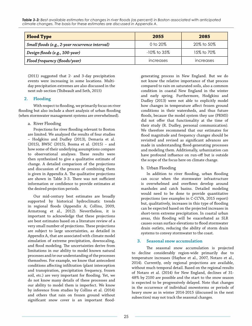
(2011) suggested that 2- and 3-day precipitation events were increasing in some locations. Multi-day precipitation extremes are also discussed in the next sub-section (Thibeault and Seth, 2015)

2. Flooding With respect to flooding, we primarily focus on river flooding but also include a short analysis of urban flooding (when stormwater management systems are overwhelmed).

a. River Flooding Projections for river flooding relevant to Boston are limited. We analyzed the results of four studies – Hodgkins and Dudley (2013), Demaria et al. (2015), BWSC (2015), Bosma et al. (2015) – and how some of their underlying assumptions compare to observational analyses. These results were then synthesized to give a qualitative estimate of change. A detailed comparison of the projections and discussion of the process of combining them is given in Appendix A. The qualitative projections are shown in Table 3-3. There was not sufficient information or confidence to provide estimates at the desired projection periods.

Our mid-century best estimates are broadly supported by historical hydroclimatic trends in regional floods (Appendix A; Collins, 2009, Armstrong et al., 2012). Nevertheless, it is important to acknowledge that these projections are best estimates based on a literature review of a very small number of projections. These projections are subject to large uncertainties, as detailed in Appendix A, that are associated with climate model simulation of extreme precipitation, downscaling, and flood modeling. The uncertainties derive from limitations in our ability to model known natural processes and/or our understanding of the processes themselves. For example, we know that antecedent conditions affecting infiltration (plant interception and transpiration, precipitation frequency, frozen soil, etc.) are very important for flooding. Yet, we do not know many details of these processes and our ability to model them is imperfect. We know by inference from studies by Collins et al. (2014) and others that rain on frozen ground without significant snow cover is an important flood-

generating process in New England. But we do not know the relative importance of that process compared to rain on saturated soils, also a common condition in coastal New England in the winter and early spring. Furthermore, Hodgkins and Dudley (2013) were not able to explicitly model how changes in temperature affect frozen ground conditions in their watersheds, and thus future floods, because the model system they use (PRMS) did not offer that functionality at the time of their study (R. Dudley, personal communication). We therefore recommend that our estimates for flood magnitude and frequency changes should be revisited and revised as significant advances are made in understanding flood-generating processes and modeling them. Additionally, urbanization can have profound influence on run-off but is outside the scope of the focus here on climate change.

b. Urban Flooding In addition to river flooding, urban flooding can occur when the stormwater infrastructure is overwhelmed and overflows develop around manholes and catch basins. Detailed modeling would need to be done to provide quantitative projections (see examples in C-CCVA, 2015 report) but, qualitatively, increases in this type of flooding can be expected based on the projected increases in short-term extreme precipitation. In coastal urban areas, this flooding will be exacerbated as SLR causes ocean surface elevations to flood stormwater drain outlets, reducing the ability of storm drain systems to convey stormwater to the coast.

3. Seasonal snow accumulation The seasonal snow accumulation is projected to decline considerably region-wide primarily due to temperature increases (Hayhoe et al., 2007, Notaro et al., 2014). Currently, only regional projections are available, without much temporal detail. Based on the regional results of Notaro et al. (2014) for New England, declines of 31-48% by 2100 are possible and the start to the snow season is expected to be progressively delayed. Note that changes in the occurrence of individual snowstorms or periods of heavy snow as in winter 2014-2015 (discussed in the next subsection) may not track the seasonal changes.

Flood Type 2055 2085

Small floods (e.g., 2-year recurrence interval) 0 to 20% 20% to 50%

Design floods (e.g., 100-year) -10% to 35% 15% to 70%

Flood frequency (floods/year) increases increases

Table 3-3:Bestavailableestimatesforchangesinriverfloods(aspercent)inBostonassociatedwithanticipatedclimatechanges.ThebasisfortheseestimatesarediscussedinAppendixA.

25

4. Snowstorms While the snow depth for the 2014-15 season set a record in Boston and surrounding communities, that was largely due to the unusually dry (for this region) nature of the snow, rather than the overall amount of water content of the snow. This large amount of dry snow was a result of an active storm period coinciding with an unusually strong and persistent period of cold temperatures. Whether global warming can, in the short term, increase mid-latitude storminess is an active but unsettled area of research (e.g., Francis and Vavrus, 2012, 2015; Liu et al., 2012; Screen and Simmonds, 2013, 2014; Barnes, 2013; Wallace et al., 2014; Cohen et al., 2014; Fischer and Knutti, 2014; Kug et al., 2015).

In terms of temperature, we have high confidence in an overall increase of temperatures both globally and in the Boston region, but the Northeast U.S. during late winter has shown some marked cold differences from the global average in recent years – and it has been suggested that this may be actually indirectly forced by global warming (e.g., Cohen et al., 2009, 2012). So while it is not clear how this period of record snow relates to climate change, it is also not clear that such events can be ruled out simply based on overall increasing temperatures. Indeed, O’Gorman (2014) has shown that changes in heavy snowfall events can be quite different from changes in annual snowfall. By 2100, in a high emissions scenario, both aspects of snowfall decrease but with much larger changes in annual snowfall than daily heavy snowfall. O’Gorman (ibid) suggests that the temperature dependencies of precipitation extremes and the rain–snow transition lead to fractional changes in snowfall extremes that are small for sufficiently large snowfall extremes in the control climate. The most extreme (~99.9 percentile) daily snowfall values are expected to respond differently to climate change as compared to precipitation extremes or mean snowfall because snowfall extremes tend to occur at temperatures in a relatively narrow range near an optimal temperature of approximately -2 degrees Celsius. For more moderate extremes, daily snowfall intensities are expected to decrease more.

The ratio of snowfall to precipitation (S/P) is a hydrologic indicator that is sensitive to climate variability and can be used to detect and monitor hydrologic responses to climatic change (Huntington et al., 2004). Huntington et al. (ibid) showed that for eleven out of twenty-one sites across New England, annual S/P decreased significantly from 1949 to 2000, and predominantly a result of decreasing snowfall. None of these sites were specific to Boston or the Boston metro area, but the 21 stations studied encompass an area from Rhode Island to Maine, surrounding the city.

While we do not have a good basis for projections at this time, the available research suggests that it is plausible that the possibility of individual heavy snowstorms will continue even as regional winters warm and seasonal snow diminishes, and that these events may perhaps (very speculatively!) even increase in the short term – the city cannot compromise its preparedness for large snowfall

events going forward.

5. Ice storms Currently, neither climate models on their own nor climate models combined with high resolution downscaling are able to realistically simulate the complex and competing processes associated with ice storms and their possible future changes (Kilma and Morgan 2015), and so climate projections do not exist for these events.

6. Drought The only drought projections available appear to be the regional projection in Hayhoe et al. (2007), so detailed projections for Boston are not possible at this time. However, Hayhoe et al. (2007) did project an increased frequency of medium and short-term droughts and extended low-flow periods in summer and these changes are at least plausible to consider for precautionary planning.

d. Open questions and data gaps

As noted in the overview and detailed in the projections section, we can project with considerable confidence that short-term extreme precipitation and flooding will increase in Boston, although the magnitude of that increase is less certain. Seasonal snowpack is very likely to decrease. Changes to individual heavy snow events, drought, and ice storms are not clear.

A large number of factors contribute to our uncertainty in these projections. Many of them are related to the complexity of the climate system and flood hydrology and the difficulties in realistically modeling them, especially with respect to local extreme precipitation mechanisms, individually, and in terms of their relationship to river flooding. These aspects of uncertainty will decrease slowly, based on general research and new generations of models. However, there are several aspects of uncertainty in these projections that can be addressed more specifically and more quickly. We recommend the following:

■ Calculation of extreme precipitation projections with dynamical downscaling applied to CMIP5 data, including the range in projections across different models. This would be an application of a more physically-based methodology to the newest data, and could give the current best estimate of the projections with reduced uncertainty bounds.

■ More extensive model diagnostics, with an emphasis on the processes that generate extreme precipitation over the Northeast U.S. that includes the greater Boston area. Understanding how well models are able to capture the relevant physical processes is critical context for assessing our confidence in the projections. This is directly related to

26

the need for more general study of extreme precipitation, so we know what processes are important. More regional research is needed, to better understand the basic processes, as well as more research on applying existing regional research to Boston.

■ Hydrologic/hydraulic modeling of urban flooding based on the recommended updated precipitation projections. This would provide a more quantitative assessment of the possible changes in this type of flooding.

■ Additional modeling of climate-sensitive, coastal New England watersheds with distributed, process-based hydrologic models that incorporate advances in modeling the freeze-thaw cycles of the soil and groundwater along with other processes.

■ Process research to better understand the relative importance of various flood-relevant antecedent conditions, especially those operating in the winter-spring period.

■ Finally, we strongly recommend updating these projections on a regular basis, to reflect both model improvements and new research. Extreme precipitation is a very active research topic and we expect our understanding to progressively improve.

4. Extreme Temperatures

a. Key findings

■ The balance of evidence over the past decade has led to successive assertions by the scientific community that global warming is not only unequivocal but also expected to grow more significant over the next several decades.

■ As expected, there is strong consensus in terms of projections of the direction of change in hot and cold extremes. There is a relatively high degree of consensus in short-term (~2030s) changes in metrics due to the fact that GHG scenarios are relatively similar over the shorter term.

■ Despite a trend toward warmer winters, the risk of frost and freeze damage continues, and has paradoxically increased over the past decade. The frequency, intensity, and duration of cold air outbreaks is expected to decrease as the

century progresses, although intense cold snaps may persist, owing to changes in jet stream patterns potentially caused by changes in the Arctic.

■ As global warming accelerates and urban areas continue to grow, high temperatures and extreme heat events will pose growing challenges even for historically colder cities like Boston. City-level activities may account for as much as 50 percent of warming and the combined effect of global warming and the urban heat island (UHI) effect appear to have increased urban temperatures faster than rural temperatures. There are important feedbacks related to UHI, such as elevated ozone formation, that may also be of concern.

■ In the absence of suitable adaptation measures, Boston’s heat-induced mortality rate may triple over the next three decades.

■ Despite projections of decreases on average, cold waves may continue to persist at 20th century intensities and durations into the late 21st century, albeit significantly less frequently. There appears to be more multimodel consensus in changes in cold days per year than in hot days. Collectively, literature on cold waves suggests that despite overall warming trends, regional preparedness cannot be compromised, even towards the end of the century.

b. Review of existing science

The balance of evidence over the past decade has led to successive assertions (IPCC, 2007; Pachauri et al., 2014) by the scientific community that global warming is not only unequivocal but also expected to grow more significant over the next several decades. Furthermore, high degrees of certainty (IPCC, 2007; Pachauri et al., 2014) have been assigned to the hypothesis that human emissions are the primary underlying cause of the warming, especially at global scales. Of all classes of climate extremes, historical changes in the statistical distribution temperature extremes have recently been most confidently attributed to human induced warming, despite remaining uncertainties in regional and local scales (Stott et al., 2016). The non-stationary trajectory of greenhouse gas emissions is clearly apparent from measurements (e.g., Olivier, 2012) while a general upward trend in global temperature is discernible over the last several decades (IPCC, 2007; Pachauri et al., 2014). Climate models suggest (e.g., Stott et al., 2010; Santer et al., 2012) that natural causes alone cannot explain the warming trend but a consideration of human emissions can. However, while global-scale (and even continental-scale, especially over the extra-tropics) average temperature trends over multi-decadal

27

to century time horizons can be delineated, uncertainties grow at progressively higher spatial or temporal resolutions and are more difficult to discern from natural variability over nearer-term projection horizons (Ganguly et al., 2015). While temperature is less variable in space and relatively more credibly projected from models than precipitation, characterizing or projecting extremes is usually more difficult than for averages. In addition, processes such as heat island effects, wind dynamics and human activity make urban extremes more difficult to understand and project.

The 2014 US National Climate Assessment (NCA, Melillo et al., 2014) pointed to increased warming and intensifying heat waves in the Northeastern US (NEUS) overall, while indicating that average temperatures in the NEUS generally decrease to the north, with distance from the coast, and at higher elevations. The temperatures in NEUS increased by almost 2˚F (0.16˚F per decade) between 1895 and 2011, while projections of future temperature increases are highly dependent on emissions scenarios (e.g., 4.5ºF to 10ºF and 3ºF to 6ºF by 2080s following the SRES A2 and B1 scenarios respectively). The frequency, intensity and duration of heat waves in the region are projected to increase with higher emissions as well.

The urban heat island effect is one of the most well documented examples of anthropogenic climate change, although few studies have been conducted for Boston specifically (notable recent exceptions include: Coutts et al., 2015; Hardin, 2015). High metropolitan concentrations of concrete and asphalt and less vegetation traps, stores, and slowly releases solar radiation (Coutts et al., 2015), making nocturnal temperatures in the region’s larger cities several degrees higher than surrounding regions. However, while heat wave research has focused on urban areas, the rural NEUS may be relatively unprepared and hence more vulnerable to heat waves (Gutierrez and LePrevost, 2016). Areas in the northern NEUS are projected to shift from having less than five to more than 15 days per year over 90°F by the 2050s under the A2 SRES scenario. The NCA further states that despite a trend toward warmer winters, the risk of frost and freeze damage continues, and has paradoxically increased over the past decade. The frequency, intensity, and duration of cold air outbreaks is expected to decrease as the century progresses, although intense cold snaps may persist, owing to changes in jet stream patterns potentially caused by changes in the Arctic. Extended warm periods in late winter or early spring, and even warmer winters in general, are more likely in Boston under climate change. While this may be better from a human comfort perspective in a city such as Boston which can get severe cold winter spells, there have been suggestions that warmer winters on the average may cause loss of species (e.g., Morris et al., 2002) and impact readiness levels, especially given the fact that cold extremes, when they occur, may continue to be at least as intense or long-lasting in the future as they have been in the recent past.

Overall, the NEUS has been witnessing a warming

trend with heat waves exacerbating, particularly in urban areas, while cold extremes have been decreasing in frequency even though they show a seemingly paradoxical trend to persist. These broad trends are projected to continue over the course of this century with the changes depending on the emissions trajectories.

Using observed station data for more than 200 urban areas across the globe, Mishra et al. (2015) showed that these areas have experienced significant increases in the number of heat waves during the period of 1973–2012, while the frequency of cold waves in those same areas declined. More specifically, almost half of the urban areas examined experienced significant increases in the number of extreme hot days, while almost two-thirds showed significant increases in the frequency of extreme hot nights. In addition, the same study (Mishra et al., 2015) found an average tendency for larger increasing trends in the number of hot days (days above the 95th percentile of temperature) in urban versus non-urban areas. As global warming accelerates and urban areas continue to grow, high temperatures and extreme heat events will pose growing challenges even for historically colder cities like Boston. Cities like Boston not only are warmer and heat faster than their surroundings because of climate change but also because of decreased vegetation, different thermal and reflective properties of urban materials, and the direct heat generated by human activities in cities. These city-level activities may account for as much as 50 percent of warming in cities (Stone et al., 2012). In the last 50 years, the combined effect of global warming and the urban heat island effect have evidently increased urban temperatures faster than rural temperatures (e.g., see figures in Stone et al., 2012).

Space-time trends and patterns in the averages and extremes of temperatures in the state of Massachusetts and the City of Boston will follow those of the NEUS as described in the NCA (Melillo et al., 2014). The changes will impact human health and thermal comfort, coastal and urban ecosystems and infrastructures, as well as the nexus of food, water and energy (Melillo et al., 2014). Thus, there is a need to understand, in the context of averages and extremes of temperature, both the changing spatiotemporal trends and patterns as well as the nature and extent of the uncertainties.

1. Principal Impacts Sectors in Boston: Public Health and Energy

A survey of climate assessment and vulnerability reports (e.g., Frumhoff et al., 2007; Horton et al., 2014; Field et al., 2012; Pachauri et al., 2014; Busch et al., 2014) and peer-reviewed literature thematically points to public health and energy as the two principal sectors in urban environments impacted by changes in temperature and temperature extremes. Hence those two are the main focus here and, along with data availability, helped drive our selection of temperature and temperature extremes derived-metrics for review in this report. While these are the two major impacts sectors, it is still important to stress that they are not the

28

only ones; see the discussion at the end of the section for more detail.

2. Geographical Boundaries of Projections Temperature and patterns of temperature extremes tend to be relatively smooth over space, as compared to other variables like precipitation. From the perspective of purely climate modeling, then, projections for mean temperature and extremes are not expected to be markedly different across different cities near Boston (e.g., Quincy, Everett, Cambridge, etc.). Hence, for temperature, many of the quantitative projections and insights embedded within this report are generalizable to other nearby cities. One important exception is the UHI effect; as discussed later, cities themselves can play a significant role in the extent of local warming and temperature extremes (Stone et al., 2012; Mishra et al., 2015). Hence we recommend that this particular phenomenon be investigated on a case-by-case (city-by-city) basis. Studies highlighted in this report have indeed principally examined the UHI effect in Boston and Cambridge (Street et al., 2013; Coutts et al., 2015; City of Cambridge, 2015; Hardin, 2015).

c. Projections

Temperature changes may be measured directly or through their impacts on stressed systems, with varying degrees of statistical credibility and usefulness. Direct measures of average temperatures may be among the most credible of climate metrics and particularly useful for model evaluation (e.g., Gleckler et al., 2008; Kumar et al., 2014) as well as for understanding the general state of the climate system, especially given the temperature dependence of precipitation and storms (Pall et al., 2007; O’Gorman et al., 2009; Sugiyama et al., 2010; Muller et al., 2011). Heat waves may be defined through threshold exceedance, which may be especially useful if the thresholds are meaningful for impacts (e.g., for survival of crops, Schlenker and Roberts, 2009) or human comfort levels and mortality (Hajat et al., 2007; Greene et al., 2011). Cold snaps may similarly consider frost thresholds such as number of frost days (Kodra et al., 2011). A large number of indices have been developed and used to assess climate conditions in the context of human health (Blazejczyk et al., 2012).

Extreme value theory may be invoked to define T-year exceedances (or shortfalls) above (below) thresholds for characterizing high or low temperature extremes (Kharin et al., 2013; Kodra et al., 2014). These measures may provide statistically valid measures for comparing models, multi-source data, or different time windows. The consecutive exceedance (falling short of) of temperatures over a low (high) threshold over successive nights (days) may define human comfort levels, sustainability of animal or plant species and stability of infrastructures (e.g., Husser, 2016).

The definitions of heat and cold, especially extremes,

may be tailored to end user needs by combining with other variables. Examples of hot or cold indices that combine variables include heat index (City of Cambridge, 2015) or wind chill (Hajat et al., 2007), which consider temperature with relative humidity or wind speed respectively. While such indices relate more directly to end use needs, the uncertainties may be higher than measures that use temperature alone and the computation of the uncertainties may be more challenging. The IPCC (2007; Pachauri et al., 2014) lists various temperature related measures that may be important from end user perspectives. Finally, the difference across areas with different levels of urbanization, or with different elevations, or proximity to coastlines and geographic features, may impact measures pertaining to city or state boundaries.

1. Heat and Cold Waves Heat and cold waves are typically (but not exclusively) defined as events exceeding specified temperature thresholds for a given minimum number of days (Peterson et al., 2013). The specific threshold and number of days vary to a small extent in literature (e.g., Barnett et al., 2012; Meehl and Tebaldi, 2004). Heat waves are a leading cause of weather-related mortality in the United States (Busch et al., 2014). They are projected to increase in intensity, duration, and frequency under climate change (Meehl and Tebaldi, 2004), albeit with relatively large uncertainty compared with mean temperature, especially at more local scales (Ganguly et al., 2009).

Even within Boston, specific definitions can vary. The City of Boston now officially defines a heat wave as 3 days in a row of maximum temperature exceeding 90°F. Meanwhile, Boston’s Commission on Affairs of the Elderly (Elderly Commission) defines a heat emergency as three consecutive days with temperatures exceeding 86°F and relative humidity exceeding 68% (Adler et al., 2010). While we are not aware of any work that has yet looked specifically at Boston area projections using either of these exact definitions, other definitions are similar and can lend insight. It is not only of interest to project the intensity but also the duration and frequency of heat waves. Ganguly et al. (2009) examined the frequency, duration, and intensity of heat waves, and Table 4-1 shows the projections for New England. Here, heat wave intensity was defined as the annual maximum of 3-day average nighttime minima, an index that has been shown to relate to public health and mortality (Meehl and Tebaldi, 2004). For duration and frequency, the study adopted a different definition of a heat wave, namely one based on the probability of occurrence. Specifically, it selected the location-specific 95th percentile of nighttime minima over the period 2000–2007 as a threshold. Any night exceeding this threshold was considered a heat wave. Duration was defined as the average number of consecutive days per year where nighttime minima exceed that threshold. Frequency was defined as the annual average number of distinct “events,” where each event is defined as one or more consecutive days, where nighttime minima exceeded

29

this threshold. For example, consider a case where there are 10 days in a year where nighttime minima exceeded the threshold. Three of those days occur consecutively; this is counted as one event. Further, the other seven days exceeding the threshold were all distinct and do not occur consecutively with others. Thus using this measurement, there is a tradeoff between frequency and duration: thus duration would be counted as 1.25 here and frequency as eight.

Notably then, there is a dependence between duration and frequency, and the apparent lack of increase in frequency in Table 4-1 is an artifact of the fact that the heat waves are longer: the total number of days of the year where a heat wave is occurring is indeed larger in the 2100s. Meehl and Tebalid (2004) analyzed output from only one CMIP3 climate model (CCSM3.0), but used multiple initial condition runs, using the SRES B1 (lowest) and A1FI (highest) GHG scenarios. Bias analysis suggested that CCSM3.0 was able to replicate historical heat wave statistics well, lending a degree of credibility to the projections. Caveats include the fact that only one (CMIP3) climate model was used and that only the ~2050s and ~2100s were explored.

Several other studies have examined heat waves as a function of how many days per year Boston (and in some cases larger regions that include the Boston area) will experience days above 90°F, 95°F, or 100°F (Houser et al., 2015; City of Cambridge, 2015; Vavrus et al., 2015). Those are also summarized in Table 4-1. Projections made by Kopp and Rasmussen (2014) can approximately be considered probabilistic 90% confidence intervals for days per year where maximum temperature exceeds 95°F obtained from CMIP5 RCP8.5, RCP6.0, RCP4.5, and RCP2.0 multimodel ensembles, computed for the entire state of Massachusetts and area-weighted by population. The authors (Houser et al., 2015; Rasmussen et al., in rev.) explain the methodology used in more complete detail. Essentially, the approach attempts to combine the merits of a simpler climate model framework, MAGICC, which provides a probabilistic perspective into global climate change but at a coarse spatial resolution, with bias-corrected and spatially disaggregated (BCSD)-downscaled CMIP5 model ensemble outputs, which alone do not comprise probabilistic projections but can provide more sufficient local resolution. The study starts with an estimated probability distribution of global mean temperatures over time from the simpler climate model (MAGICC). It uses this distribution to weight local projections of monthly temperature and precipitation from downscaled CMIP5 global climate models. In cases where the CMIP5 models do not represent the tails of the MAGICC probability distribution well, “surrogate” models (scaled versions of CMIP5 models) are employed to ensure the tails of the probability distribution are represented. Finally, it uses historical relationships in observed (using Global Historical Climatological Network data) data to translate inferred monthly values to daily values. Projections were made for the entire 21st century, with a focus on the intervals 2020-2039, 2040-2059, and 2080-2099. The results provide a potentially richer probabilistic representation of hot days. One caveat is

that there was no explicit out-of-sample predictive validation of the results, e.g., against held-out historical data. However, results were bias-corrected relative to historical data. The same study performs this analysis to also infer probabilistic projections for seasonal average temperature and cold waves (days below 32°F) as well; both are included in Table 4-1. This includes the 5th and 95th percentiles.

Another recent study (Vavrus et al. 2015) defined “hot days” as days where maximum temperatures reach at least 90°F. The study used an approach based on downscaling and statistical bootstrapping to probabilistically quantify projected changes. This study leveraged an ensemble of 13 CMIP3 GCM projections run with the mid-range SRES A1B emissions scenario. The multimodel median projected increase from the period 1961-2000 to the 2050s in hot days in the Greater Boston area is approximately an increase of 15-25 days. Each CMIP3 model was downscaled using high-resolution gridded observed data. The multimodel minimum expected increase in hot days was depicted as approximately 5-15, while the uppermost model shows an increase of as much as 45-55 days per year. A bootstrap created a distribution of multimodel means; the probabilistic aspect of this only quantifies uncertainty in the central tendency of the models, not necessarily uncertainty in the full range of outcomes. This effectively discounts outlying models, not based on any evidence that those models are less credible (other than being very different than an “average” model). For that reason, here we show the multimodel minima and maxima in Table 4-1, which arguably present a more complete plausible range. The study also repeated this analysis for “cold days” or days where minimum temperature hits 0°F or less.

The City of Cambridge (City of Cambridge, 2015) analyzed heat waves as projected days above 90°F and 100°F via collaboration with Kleinfelder and ATMOS research. Projections utilize 4 CMIP3 and 9 CMIP5 models via two different GHG scenarios. For CMIP3, B1 and A1Fi were used, and for CMIP5, RCP4.5 and RCP8.5 were used, respectively representing less and more GHG intensive trajectories. Ranges provided here represent the full range of both generations of models and all scenarios. The B1 scenario might be considered overly optimistic. If so, in the 2070s, a range of 35-90 days per year above 90°F might be considered more appropriate compared to 11 days per year in the period 1971-2000. Each scenario gives a range in which to measure expectations. Either way, further into the future uncertainty grows more as a function of socioeconomic trajectory uncertainty. Expected days above 90°F were stated to be 55-70 in the 2070s and 30-44 under the high and low scenarios, respectively. For the 2030s the expected range is 20-30, but note that that appendix also depicts an uppermost bound of 40. Statistical downscaling was done using an asynchronous regional regression model (Stoner et al., 2013).

All of the above definitions of heat waves are based purely on temperature. However, other variables, including humidity, cloudiness, and wind conditions, also characterize the air conditions that are associated with public health

30

concerns and mortality (Greene et al., 2011). To gather an initial sense, one recent study (Petkova et al., 2013) estimates that Boston’s heat-induced mortality rate may triple over the next three decades. One recent study (Greene et al., 2011) developed projections for so-called summertime Excessive Heat Events (EHEs) specifically for Boston among a collection of other cities in the United States. The study’s projections reflect that, rather than responding in isolation to individual weather elements (e.g., maximum temperature), human health (mortality) is affected by the simultaneous interactions from a combination of meteorological conditions (e.g., temperature, humidity, cloud cover, and wind speed). They use a spatial synoptic classification (Sheridan, 2002) method to categorize weather conditions into a type in each city, for each day. The SSC is essentially a dimensionality reduction approach; it uses a range of meteorological variables as inputs and classifies each day at a particular location into one of several distinct weather types. Every day’s weather is either classified into one of six main weather types or as a transition between two different weather types.

There are two weather types that are associated with mortality rates that are significantly higher than normal. They include: Dry tropical (DT): The hottest weather type. For summer, temperatures usually exceed 95°F and sometimes exceed 100°F. This weather type is also generally associated with low cloud cover humidity, which is in turn associated with the possibility of dehydration. Next, Moist Tropical (MT): very warm and humid air, sometimes associated with summer thunderstorms. This weather type is associated with the highest apparent temperature values, and is often quite muggy and uncomfortable. Since MT is often quite prevalent in the summer, this weather type was subdivided to more closely establish the heat–mortality relationship. Thus, a subset of MT was defined: Moist tropical plus (MT1): These are particularly hot and humid subsets of the MT weather type. Dewpoint temperatures are very high, with temperatures of 90°F, and overnight temperatures are the warmest of any of the six weather types. This is an important case to consider, where the climate extreme is not purely based on one variable but is a combination, where temperature plays a prominent role. There are several important caveats, however. The study (Greene et al., 2011) derives weather types from only one CMIP3 model (Parallel Climate Model) into the future to project the number of EHEs for Boston among other cities, as well as extrapolate the number of estimated mortalities. While it only uses one GCM, the study did at least use two SRES scenarios, B1 and A1FI, to approximate some information on uncertainty. There are many caveats associated with this: there is uncertainty not captured in terms of multi-model uncertainty or initial conditions. There is also no depiction of goodness of fit or uncertainty in the mortality regression. We opted to leave the mortality projections out of this work since they are beyond the scope of this particular report, but they may be useful to investigate in subsequent vulnerability assessments.

Generally, fewer studies and projections are available for cold waves, likely owing to the fact that they are expected

to generally decrease in intensity, duration, and especially frequency at regional scales (Kodra et al., 2011; Kodra and Ganguly, 2014). Results obtained from an ensemble of nine CMIP3 global climate models run under the moderate SRES A1B scenario show that despite projections of decreases on average, cold waves may continue to persist at 20th century intensities and durations into the late 21st century, albeit significantly less frequently (Kodra et al., 2011). As a caveat, under more intense GHG scenarios, which were not explored, it is very possible that the intensity and duration dimensions would not show the same levels of projected persistence.

In addition, more recent research with 14 CMIP5 models using RCP4.5 (Kodra and Ganguly, 2014) suggests asymmetry in projections of heat waves and cold spells, wherein in both tails the warmest temperatures may increase more than the coldest, especially in the Northern Hemisphere. Vavrus et al. (2015) utilized the same methodology and data discussed above to project days below 0°F, as well. Their results suggest that the number of cold days will decrease but not disappear in the 2050s (Table 4-1). The authors (Vavrus et al., 2015) also mention that they found more multimodel consensus in changes in cold days per year than in hot days. These projections are based on the mid-range SRES A1B GHG scenario, the same as in Kodra et al. (2011). Houser et al. (2015) and Rasmussen et al. (in rev.) estimated analogous probabilistic projections for days per year where minimum temperature falls below 32°F using all the same suite of models, data and methodology detailed previously. Table 4-1 summarizes 90% confidence intervals generated from that study. Results imply a strong decline but also strongly suggest the likelihood of a persistent, high number of days below 32°F late into the 21st century. This is consistent with the other work summarized here. Collectively, literature on cold waves suggests that despite overall warming trends, regional preparedness cannot be compromised, even towards the end of the century.

2. Heating and Cooling Degree Days Heating or cooling degree days (HDD and CDD, respectively) (Amato et al., 2005; Petri and Caldeira, 2015) are measures that relate to energy usage for climate control related to cold or hot weather respectively. Typically, a balance point temperature is defined above which cooling takes place and below which heating takes place. It is standard practice to assume 65°F (18.3°C) as the balance point temperature to allow for comparisons across time or space, holding the reference temperature constant (e.g., Petri & Caldeira, 2015). In reality, however, heating and cooling are adjusted gradually within ranges around separate balance points for cold and hot conditions (Amato et al., 2005), and different places exhibit different temperature sensitivities. For example, one study (Amato et al., 2005) estimated balance point temperatures specifically in metro Boston for electricity consumption in the residential and commercial sectors, respectively, of 60°F (15.6°C) and 55°F (12.8°C), owing to adaptation of the building stock, proliferation of air conditioning, and behavioral parameters. Table 4-1

31

allows for partial comparison of projections derived from different thresholds (Amato et al., 2005; Petri and Caldeira, 2015). There are substantial differences between the two and important implications of insights that could be derived depending on which threshold is used.

To complement the Amato et al. (2005) study, we used DegreeDays.net to estimate CDD at the 60°F baseline (2015). This site actually pulls data from KBOS (Boston Logan Airport) via www.wunderground.com (WeatherUnderground), using Dec 2012 - Nov 2015 data. There is a significant difference between the more oft-used 65°F baseline. It is most important to point out that specific projections at the thresholds considered to be appropriate for Boston (Amato et al., 2005) have only been made out to the 2030s. Petri and Caldeira (2015)’s historical baseline for HDD and CDD relies on interpolated NOAA 30-year daily degree-day normals. Multimodel medians from 28 CMIP5 models, using RCP8.5 runs, were used for 2016-2035 (~2030) 2080-2099 (~2100) projections (4). However, unlike Amato et al. (2005) these are not adjusted to the 60°F baseline that was deemed appropriate specifically for Boston’s building stock. Rather this study uses the standard 65°F baseline. Although this study used 28 CMIP5 models, it only used ensemble median projections and did not include any measurements of uncertainty in degree days.

It is worth noting that the American Climate Prospectus (Houser et al., 2015) developed population-weighted probabilistic projections of HDD and CDD for Massachusetts (and all other 49 states) using the conventional 65°F baseline. However, they do not appear to have been made directly publicly available. Rather, that study harnesses those HDD and CDD projections with an energy model and develops projections for changes in retail electricity sales and energy expenditures (Houser et al., 2015). While these are outside the scope of this particular report because they go beyond purely assessing climate risk factors, they are worth highlighting here and considering in subsequent economic and vulnerability assessments. While HDD is likely to increase based on projections, and perhaps will at least “offset” projected increases in CDD in terms of annual totals under climate change, it is important to note that a 1% increase in CDDs have historically had a significantly larger effect on energy demand than the same for HDDs (Houser et al., 2015).

For examining the likely effects of climate change on total annual HDDs and CDDs, stakeholders may find it useful to rely on a combination of insights from Petri and Caldeira (2015) and Houser et al. (2015), since they are relatively complete in terms of data availability. However, those insights and projections must be balanced carefully with the fact that they were not calculated using Boston-specific baseline temperatures (Amato et al., 2005). Differences or percentage differences for future time periods projected from Petri and Caldeira (2015) and Houser et al. (2015) may approximate more meaningful values than the absolute values projected. Future research might consider

developing a full set of projections for HDDs and CDDs that use the more appropriate Boston baseline temperature.

3. The Urban Heat Island Effect The Urban Heat Island (UHI) effect is a well-recognized phenomenon in cities wherein the concrete, steel and other building materials that compose the built environment generally retain more heat and create a significantly hotter environment than suburban and rural areas (Faber et al., 2014). The UHI effect can give cause for concern for urban public health and mortality (e.g., Dousset et al., 2011), especially among aging and economically disadvantaged populations. It can also have important implications for summer peak energy demand and air quality (Coutts et al., 2015). The UHI has been estimated to be responsible for 5-10% of peak electric demand for cooling (Akbari 2005 - http://www.inive.org/members_area/medias/pdf/Inive/palenc/2005/Akbari.pdf). A recent study conducted using data collected specifically from the Greater Boston area (Street et al., 2013) estimates the measurable effect on energy required to cool equivalent buildings in an urban compared to a rural or suburban area. The authors use Central Square in Cambridge, MA as the urban site of choice. Results show that a small office (small residential) building located at Boston-Logan International Airport (KBOS) would use 29% (5%) less energy for cooling per square meter than the same building placed in Central Square. Similarly, the same small office (small residential) building located at Hanscom Air Force Base (KBED) would use 18% (4%) less energy for cooling than in Central Square. On the other hand, the UHI can have energy demand benefits in the winter. The same small office (small residential) building located at KBOS would use 4% (16%) more energy for heating than the same building in Central Square. Finally, the same small office building located at KBED would use 15% (18%) more energy for cooling compared to the same building in Central Square (Street et al., 2013).

A report prepared for The Trust for Public Land (Coutts et al., 2015) explored the UHI effect in Boston in the context of pockets of high vulnerability and potential mitigation solutions. This is a useful resource for vulnerability assessment and mitigation planning, although climate projections and climate risk factor specifics are explicitly not included in its maps. Another recent study (Hardin, 2015) examined the current UHI effect in four cities, including Boston. That study compiles estimates on full day, daytime, and nighttime average UHI intensities and standard deviations by multiple weather types. Although for conciseness they are not tabulated here, that detailed table is valuable and can be found in Hardin (2015) – https://ttu-ir.tdl.org/ttu-ir/bitstream/handle/2346/63661/HARDIN-THESIS-2015.pdf?sequence=1.

To our knowledge, the City of Cambridge (City of Cambridge, 2015) constructed the only report that lent a Boston area-specific perspective into the UHI under projections of climate change. The report provides detailed maps that leverage satellite imagery in one

32

online appendix (City of Cambridge, 2015 - http://www.cambr idgema.gov/CDD/Projects/Cl imate/~/media /CEECF015AB2645C1811C33F707CEA85A.ashx) and methodological details in another (City of Cambridge, 2015 - http://www.cambridgema.gov/CDD/Projects/Climate/~/media/007A3255079540399C25A78038B961A9.ashx). Maps are provided for the 2030s and the 2070s, for both ambient air temperature and a heat index that incorporates both ambient air temperature and humidity. Essentially, these were built using hypothetical scenarios of the UHI under climate change: simple assumptions about what characteristics could comprise a heat wave in both of those climatologies.

While this approach may be useful, it is suggestive and not probabilistic, and does not directly consider climate model output. The results are also limited to the City of Cambridge and do not cover Boston or other nearby cities. It may be possible to combine multiple (potentially downscaled) climate model outputs with such a methodology (City of Cambridge, 2015) to obtain ensembles of projected effects of UHI in the future. This is a direction that future researchers may wish to explore given the likely importance of UHI in exacerbating the impacts of climate change in cities like Boston.

Stakeholders may wish to rely on a combination of these studies in the near term: Street et al. (2013) yields initial insights for energy usage differentials in urban versus rural Boston areas; Hardin (2015) provides detailed numeric and geospatial data on current Boston metro area UHI effects under multiple spatial synoptic weather types; Coutts et al. (2015) provides detailed current urban heat vulnerability geospatial data for Boston; and Rossi et al. (2015) provides current and hypothetical future physical UHI effects for Cambridge.

Although at first glance, the urban heat island problem seems – at the city-scale – static in time and linear in the sense that causes are independent from effects, there are important feedback mechanisms that unfold over the long term. Elevated ozone formation due to prolonged hot periods can have adverse effects on plants, which can trigger a reinforcing feedback loop. Over the long term, increases in land use conversion along the urban fringe will further reduce evapotranspiration. Persistent temperature increase in cities can give rise to increases in air conditioner ownership. Also, the choice of building materials, city albedo, and efficiency of appliances can change, as people try to adapt to increased temperatures; some choices can reduce the urban heat island effect. Green infrastructure investments could hypothetically significantly reduce burdens on urban water and energy systems, thereby potentially mitigating energy demand (e.g., Cherrier et al., 2016.) Depending on the relative climate change compared to other cities, population movements can occur. Increased temperatures can make some northern cities more livable, attracting immigration. This pressure would lead to an increase in the size of these cities and/or decrease their urban vegetation to make space

for larger populations, both of which contribute to the urban heat island. If, at the same time, the city will not (or cannot) invest in public transportation, travel-related heat generation would increase even more.

d. Discussion and data gaps

Average temperature and (to a lesser extent) temperature extremes are generally considered the most reliably projected by climate models. This section of the report and its data implies:

■ Expectedly, there is strong consensus in terms of projections of sign of change in hot and cold extremes.

■ There is a relatively high degree of consensus in short-term (~2030s) changes in metrics, regardless of whether an anthropogenic signal can be readily delineated from natural variability. This is owing to the fact that GHG scenarios are relatively similar over the shorter term.

■ There is considerable uncertainty in the specific trajectory of especially hot extremes and temperature-derived metrics (like cooling degree days) further into the future.

■ In some cases, it can be important to choose metrics that are appropriate specifically for Boston (see section on Heating and Cooling Degree Days, where a simple threshold choice can have significantly different implications than another).

■ Many stakeholders, especially those seeking climate adaptation solutions with estimable cost-risk tradeoffs, would be best equipped with probabilistic climate projections rather than simply best estimates. Generally speaking, these rarely exist as data, tools or in literature. Exceptions include work highlighted and presented here (e.g., Houser et al., 2015; Rasmussen et al. (in rev.); Petri and Caldeira, 2015). Even these are conditioned on GHG scenarios, which themselves cannot readily be treated probabilistically because they are “storylines” about plausible futures. However, they represent a useful direction for delivering actionable insights to local stakeholders. Opportunities may exist for developing novel physics-guided data science methods for probabilistic modeling as well (for details, see Ganguly et al., 2014; Faghmous and Kumar, 2014).

■ The temperature projections tabulated in this

33

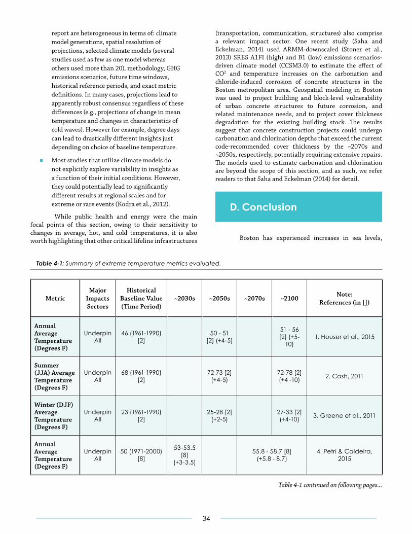
report are heterogeneous in terms of: climate model generations, spatial resolution of projections, selected climate models (several studies used as few as one model whereas others used more than 20), methodology, GHG emissions scenarios, future time windows, historical reference periods, and exact metric definitions. In many cases, projections lead to apparently robust consensus regardless of these differences (e.g., projections of change in mean temperature and changes in characteristics of cold waves). However for example, degree days can lead to drastically different insights just depending on choice of baseline temperature.

■ Most studies that utilize climate models do not explicitly explore variability in insights as a function of their initial conditions. However, they could potentially lead to significantly different results at regional scales and for extreme or rare events (Kodra et al., 2012).

While public health and energy were the main focal points of this section, owing to their sensitivity to changes in average, hot, and cold temperatures, it is also worth highlighting that other critical lifeline infrastructures

MetricMajor

Impacts Sectors

Historical Baseline Value (Time Period)

~2030s ~2050s ~2070s ~2100 Note: References (in [])

Annual Average Temperature (Degrees F)

Underpin All

46 (1961-1990) [2]

50 - 51 [2] (+4-5)

51 - 56 [2] (+5-

10)1. Houser et al., 2015

Summer (JJA) Average Temperature (Degrees F)

Underpin All

68 (1961-1990) [2]

72-73 [2] (+4-5)

72-78 [2] (+4 -10)

2. Cash, 2011

Winter (DJF) Average Temperature (Degrees F)

Underpin All

23 (1961-1990) [2]

25-28 [2] (+2-5)

27-33 [2] (+4-10)

3. Greene et al., 2011

Annual Average Temperature (Degrees F)

Underpin All

50 (1971-2000) [8]

53-53.5 [8]

(+3-3.5)

55.8 - 58.7 [8] (+5.8 - 8.7)

4. Petri & Caldeira, 2015

(transportation, communication, structures) also comprise a relevant impact sector. One recent study (Saha and Eckelman, 2014) used ARMM-downscaled (Stoner et al., 2013) SRES A1FI (high) and B1 (low) emissions scenarios-driven climate model (CCSM3.0) to estimate the effect of CO2 and temperature increases on the carbonation and chloride-induced corrosion of concrete structures in the Boston metropolitan area. Geospatial modeling in Boston was used to project building and block-level vulnerability of urban concrete structures to future corrosion, and related maintenance needs, and to project cover thickness degradation for the existing building stock. The results suggest that concrete construction projects could undergo carbonation and chlorination depths that exceed the current code-recommended cover thickness by the ~2070s and ~2050s, respectively, potentially requiring extensive repairs. The models used to estimate carbonation and chlorination are beyond the scope of this section, and as such, we refer readers to that Saha and Eckelman (2014) for detail.

D. Conclusion

Boston has experienced increases in sea levels,

Table 4-1: Summaryofextremetemperaturemetricsevaluated.

Table 4-1 continued on following pages...

34

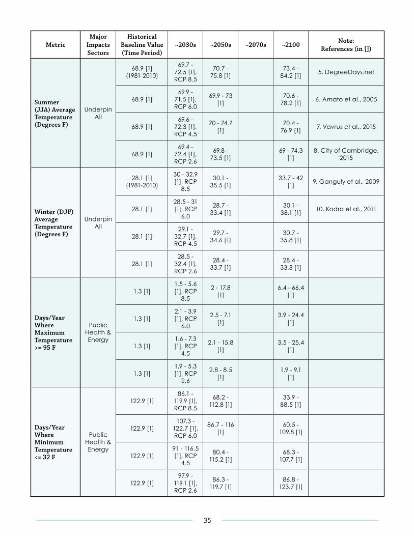
MetricMajor

Impacts Sectors

Historical Baseline Value (Time Period)

~2030s ~2050s ~2070s ~2100 Note: References (in [])

Summer (JJA) Average Temperature (Degrees F)

Underpin All

68.9 [1] (1981-2010)

69.7 - 72.5 [1], RCP 8.5

70.7 - 75.8 [1]

73.4 - 84.2 [1]

5. DegreeDays.net

68.9 [1]69.9 -

71.5 [1], RCP 6.0

69.9 - 73 [1]

70.6 - 78.2 [1]

6. Amato et al., 2005

68.9 [1]69.6 -

72.3 [1], RCP 4.5

70 - 74.7 [1]

70.4 - 76.9 [1]

7. Vavrus et al., 2015

68.9 [1]69.4 -

72.4 [1], RCP 2.6

69.8 - 73.5 [1]

69 - 74.3 [1]

8. City of Cambridge, 2015

Winter (DJF) Average Temperature (Degrees F)

Underpin All

28.1 [1] (1981-2010)

30 - 32.9 [1], RCP

8.5

30.1 - 35.5 [1]

33.7 - 42 [1]

9. Ganguly et al., 2009

28.1 [1]28.5 - 31 [1], RCP

6.0

28.7 - 33.4 [1]

30.1 - 38.1 [1]

10. Kodra et al., 2011

28.1 [1]29.1 -

32.7 [1], RCP 4.5

29.7 - 34.6 [1]

30.7 - 35.8 [1]

28.1 [1]28.5 -

32.4 [1], RCP 2.6

28.4 - 33.7 [1]

28.4 - 33.8 [1]

Days/Year Where Maximum Temperature >= 95 F

Public Health & Energy

1.3 [1]1.5 - 5.6 [1], RCP

8.5

2 - 17.8 [1]

6.4 - 66.4 [1]

1.3 [1]2.1 - 3.9 [1], RCP

6.0

2.5 - 7.1 [1]

3.9 - 24.4 [1]

1.3 [1]1.6 - 7.3 [1], RCP

4.5

2.1 - 15.8 [1]

3.5 - 25.4 [1]

1.3 [1]1.9 - 5.3 [1], RCP

2.6

2.8 - 8.5 [1]

1.9 - 9.1 [1]

Days/Year Where Minimum Temperature <= 32 F

Public Health & Energy

122.9 [1]86.1 -

119.9 [1], RCP 8.5

68.2 - 112.8 [1]

33.9 - 88.5 [1]

122.9 [1]107.3 -

122.7 [1], RCP 6.0

86.7 - 116 [1]

60.5 - 109.8 [1]

122.9 [1]91 - 116.5 [1], RCP

4.5

80.4 - 115.2 [1]

68.3 - 107.7 [1]

122.9 [1]97.9 -

119.1 [1], RCP 2.6

86.3 - 119.7 [1]

86.8 - 123.7 [1]

35

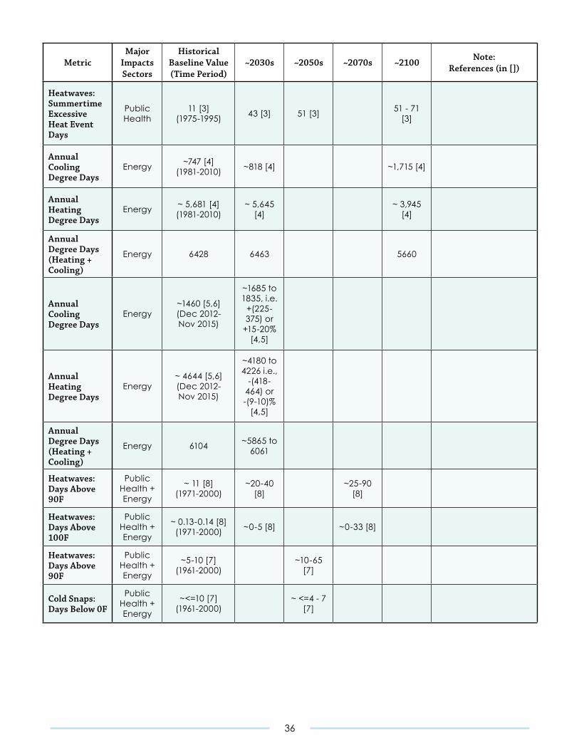
MetricMajor

Impacts Sectors

Historical Baseline Value (Time Period)

~2030s ~2050s ~2070s ~2100 Note: References (in [])

Heatwaves: Summertime Excessive Heat Event Days

Public Health

11 [3] (1975-1995)

43 [3] 51 [3]51 - 71

[3]

Annual Cooling Degree Days

Energy~747 [4]

(1981-2010)~818 [4] ~1,715 [4]

Annual Heating Degree Days

Energy~ 5,681 [4] (1981-2010)

~ 5,645 [4]

~ 3,945 [4]

Annual Degree Days (Heating + Cooling)

Energy 6428 6463 5660

Annual Cooling Degree Days

Energy~1460 [5,6] (Dec 2012- Nov 2015)

~1685 to 1835, i.e.

+(225-375) or

+15-20% [4,5]

Annual Heating Degree Days

Energy~ 4644 [5,6] (Dec 2012- Nov 2015)

~4180 to 4226 i.e.,

-(418-464) or -(9-10)%

[4,5]

Annual Degree Days (Heating + Cooling)

Energy 6104~5865 to

6061

Heatwaves: Days Above 90F

Public Health + Energy

~ 11 [8] (1971-2000)

~20-40 [8]

~25-90 [8]

Heatwaves: Days Above 100F

Public Health + Energy

~ 0.13-0.14 [8] (1971-2000)

~0-5 [8] ~0-33 [8]

Heatwaves: Days Above 90F

Public Health + Energy

~5-10 [7] (1961-2000)

~10-65 [7]

Cold Snaps: Days Below 0F

Public Health + Energy

~<=10 [7] (1961-2000)

~ <=4 - 7 [7]

36

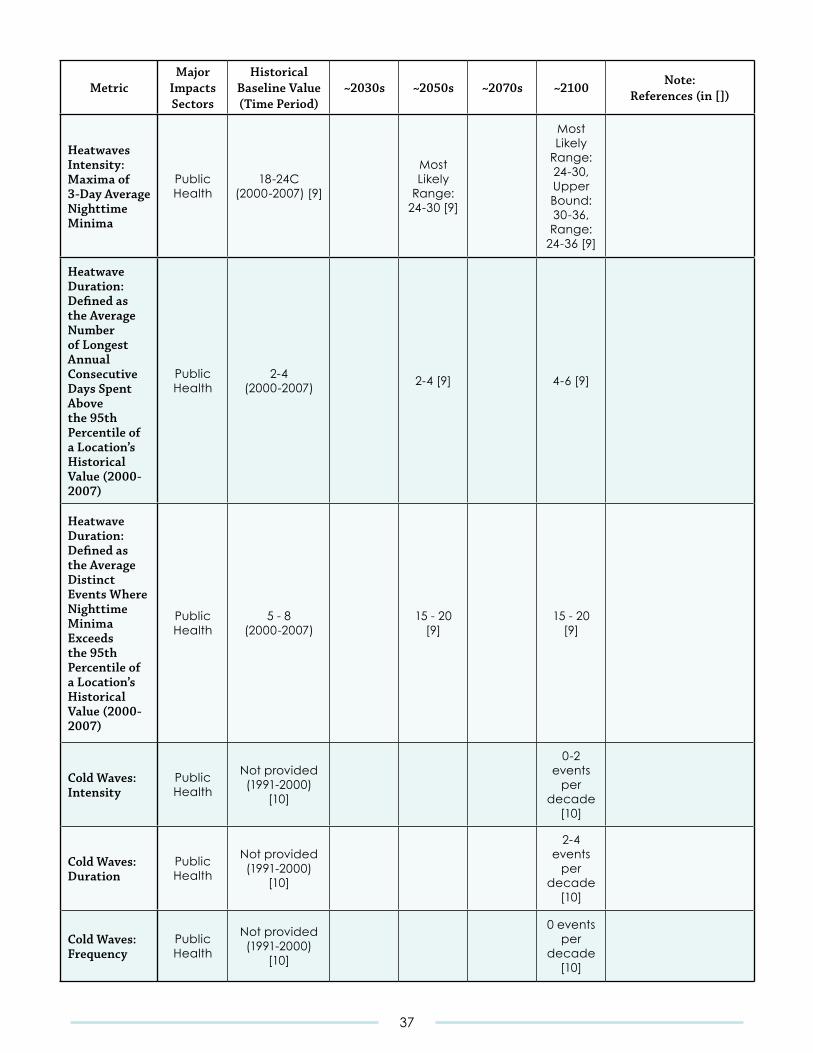
MetricMajor

Impacts Sectors

Historical Baseline Value (Time Period)

~2030s ~2050s ~2070s ~2100 Note: References (in [])

Heatwaves Intensity: Maxima of 3-Day Average Nighttime Minima

Public Health

18-24C (2000-2007) [9]

Most Likely

Range: 24-30 [9]

Most Likely

Range: 24-30, Upper Bound: 30-36, Range:

24-36 [9]

Heatwave Duration: Defined as the Average Number of Longest Annual Consecutive Days Spent Above the 95th Percentile of a Location’s Historical Value (2000-2007)

Public Health

2-4 (2000-2007)

2-4 [9] 4-6 [9]

Heatwave Duration: Defined as the Average Distinct Events Where Nighttime Minima Exceeds the 95th Percentile of a Location’s Historical Value (2000-2007)

Public Health

5 - 8 (2000-2007)

15 - 20 [9]

15 - 20 [9]

Cold Waves: Intensity

Public Health

Not provided (1991-2000)

[10]

0-2 events

per decade

[10]

Cold Waves: Duration

Public Health

Not provided (1991-2000)

[10]

2-4 events

per decade

[10]

Cold Waves: Frequency

Public Health

Not provided (1991-2000)

[10]

0 events per

decade [10]

37

extreme high precipitation, and extreme high temperature. Past changes in the frequencies and intensities of extratropical and tropical storms have been difficult to quantify. Projections of future changes of these climate characteristics are uncertain, due to lack of complete knowledge of the climate system (as reflected in differences in the results of multiple GCMs) and of future GHG emissions, with the uncertainty growing over time. There is considerably less uncertainty in the projections early in the 21st century compared to later in the century. We can, however expect to see continued increases in sea levels, extreme precipitation, and extreme high temperatures in the future and we can provide quantitative estimates suitable for planning for many parameters. Even though we cannot quantify with confidence possible changes in storms, by using probabilities of existing storm surge conditions, we have developed useable projections of future coastal flood conditions. Given an emission scenario, changes in extreme temperature and precipitation are presented in most cases as ranges of future conditions while probabilistic estimates of sea level rise and coastal flooding elevations are presented.

Many of the uncertainties related to lack of complete knowledge of the climate system will decrease over time as more research is conducted. In addition, the range in possible GHG emission scenarios will also decrease over time if global agreements on emission targets are implemented. We recommend that the climate change and SLR projections in this report be updated at least every two years using the mechanism suggested in this report.

38

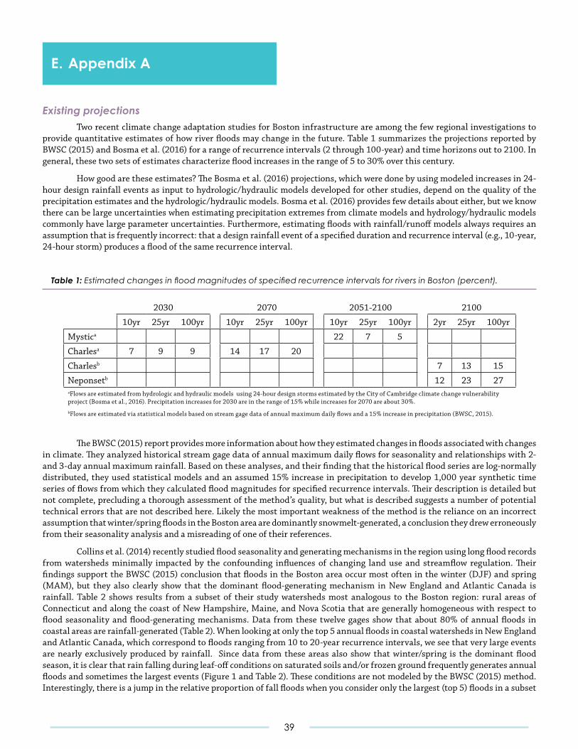
E. Appendix A

Existing projections Two recent climate change adaptation studies for Boston infrastructure are among the few regional investigations to provide quantitative estimates of how river floods may change in the future. Table 1 summarizes the projections reported by BWSC (2015) and Bosma et al. (2016) for a range of recurrence intervals (2 through 100-year) and time horizons out to 2100. In general, these two sets of estimates characterize flood increases in the range of 5 to 30% over this century.

How good are these estimates? The Bosma et al. (2016) projections, which were done by using modeled increases in 24-hour design rainfall events as input to hydrologic/hydraulic models developed for other studies, depend on the quality of the precipitation estimates and the hydrologic/hydraulic models. Bosma et al. (2016) provides few details about either, but we know there can be large uncertainties when estimating precipitation extremes from climate models and hydrology/hydraulic models commonly have large parameter uncertainties. Furthermore, estimating floods with rainfall/runoff models always requires an assumption that is frequently incorrect: that a design rainfall event of a specified duration and recurrence interval (e.g., 10-year, 24-hour storm) produces a flood of the same recurrence interval.

2030 2070 2051-2100 2100

10yr 25yr 100yr 10yr 25yr 100yr 10yr 25yr 100yr 2yr 25yr 100yr

Mystica 22 7 5

Charlesa 7 9 9 14 17 20

Charlesb 7 13 15

Neponsetb 12 23 27aFlows are estimated from hydrologic and hydraulic models using 24-hour design storms estimated by the City of Cambridge climate change vulnerability project (Bosma et al., 2016). Precipitation increases for 2030 are in the range of 15% while increases for 2070 are about 30%.

bFlows are estimated via statistical models based on stream gage data of annual maximum daily flows and a 15% increase in precipitation (BWSC, 2015).

Table 1: EstimatedchangesinfloodmagnitudesofspecifiedrecurrenceintervalsforriversinBoston(percent).

The BWSC (2015) report provides more information about how they estimated changes in floods associated with changes in climate. They analyzed historical stream gage data of annual maximum daily flows for seasonality and relationships with 2- and 3-day annual maximum rainfall. Based on these analyses, and their finding that the historical flood series are log-normally distributed, they used statistical models and an assumed 15% increase in precipitation to develop 1,000 year synthetic time series of flows from which they calculated flood magnitudes for specified recurrence intervals. Their description is detailed but not complete, precluding a thorough assessment of the method’s quality, but what is described suggests a number of potential technical errors that are not described here. Likely the most important weakness of the method is the reliance on an incorrect assumption that winter/spring floods in the Boston area are dominantly snowmelt-generated, a conclusion they drew erroneously from their seasonality analysis and a misreading of one of their references.

Collins et al. (2014) recently studied flood seasonality and generating mechanisms in the region using long flood records from watersheds minimally impacted by the confounding influences of changing land use and streamflow regulation. Their findings support the BWSC (2015) conclusion that floods in the Boston area occur most often in the winter (DJF) and spring (MAM), but they also clearly show that the dominant flood-generating mechanism in New England and Atlantic Canada is rainfall. Table 2 shows results from a subset of their study watersheds most analogous to the Boston region: rural areas of Connecticut and along the coast of New Hampshire, Maine, and Nova Scotia that are generally homogeneous with respect to flood seasonality and flood-generating mechanisms. Data from these twelve gages show that about 80% of annual floods in coastal areas are rainfall-generated (Table 2). When looking at only the top 5 annual floods in coastal watersheds in New England and Atlantic Canada, which correspond to floods ranging from 10 to 20-year recurrence intervals, we see that very large events are nearly exclusively produced by rainfall. Since data from these areas also show that winter/spring is the dominant flood season, it is clear that rain falling during leaf-off conditions on saturated soils and/or frozen ground frequently generates annual floods and sometimes the largest events (Figure 1 and Table 2). These conditions are not modeled by the BWSC (2015) method. Interestingly, there is a jump in the relative proportion of fall floods when you consider only the largest (top 5) floods in a subset

39

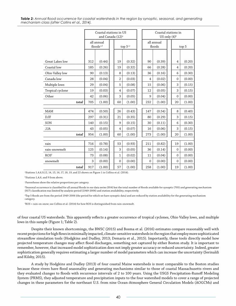
of four coastal US watersheds. This apparently reflects a greater occurrence of tropical cyclones, Ohio Valley lows, and multiple lows in this sample (Figure 1; Table 2).

Despite their known shortcomings, the BWSC (2015) and Bosma et al. (2016) estimates compare reasonably well with recent projections for high flows in minimally impacted, climate-sensitive watersheds in the region that employ more sophisticated streamflow simulation tools (Hodgkins and Dudley, 2013; Demaria et al., 2015). Importantly, these tools directly model how projected temperature changes may affect flood discharges, something not captured by either Boston study. It is important to remember, however, that increased model sophistication does not imply greater accuracy or reduced uncertainty. Indeed, greater sophistication generally requires estimating a larger number of model parameters which can increase the uncertainty (Serinaldi and Kilsby, 2015).

A study by Hodgkins and Dudley (2013) of four coastal Maine watersheds is most comparable to the Boston studies because these rivers have flood seasonality and generating mechanisms similar to those of coastal Massachusetts rivers and they evaluated changes to floods with recurrence intervals of 2 to 100 years. Using the USGS Precipitation-Runoff Modeling System (PRMS), they adjusted temperature and precipitation inputs to the four watershed models to cover a range of projected changes in these parameters for the northeast U.S. from nine Ocean-Atmosphere General Circulation Models (AOGCMs) and

Coastal stations in US and Canada (12)a

Coastal stations in US only (4)b

all annual floodsc,d top 5c,e

all annual floods top 5

Great Lakes low 312 (0.44) 19 (0.32) 90 (0.39) 4 (0.20)

Coastal low 185 (0.26) 19 (0.32) 66 (0.28) 4 (0.20)

Ohio Valley low 90 (0.13) 8 (0.13) 36 (0.16) 6 (0.30)

Canada low 28 (0.04) 2 (0.03) 4 (0.02) 0 (0.00)

Multiple lows 29 (0.04) 5 (0.08) 15 (0.06) 3 (0.15)

Tropical cyclone 19 (0.03) 4 (0.07) 12 (0.05) 3 (0.15)

Other 42 (0.06) 3 (0.05) 9 (0.04) 0 (0.00)

total 705 (1.00) 60 (1.00) 232 (1.00) 20 (1.00)

MAM 474 (0.50) 26 (0.43) 147 (0.54) 8 (0.40)

DJF 297 (0.31) 21 (0.35) 80 (0.29) 3 (0.15)

SON 140 (0.15) 9 (0.15) 30 (0.11) 6 (0.30)

JJA 43 (0.05) 4 (0.07) 16 (0.06) 3 (0.15)

total 954 (1.00) 60 (1.00) 273 (1.00) 20 (1.00)

rain 716 (0.78) 53 (0.93) 211 (0.82) 19 (1.00)

rain-snowmelt 125 (0.14) 3 (0.05) 36 (0.14) 0 (0.00)

ROSf 73 (0.08) 1 (0.02) 11 (0.04) 0 (0.00)

snowmelt 3 (0.00) 0 (0.00) 0 (0.00) 0 (0.00)

total 917 (1.00) 57 (1.00) 258 (1.00) 19 (1.00)aStations 1,4,6,9,12, 14, 15, 16, 17, 18, 19, and 22 shown on Figure 1 in Collins et al. (2014).

bStations 1,4,6, and 9 from above.

cParentheses show the relative proportions per category.

dSeasonal occurrence is classified for all annual floods in our data series (954) but the total number of floods available for synoptic (705) and generating mechanism (917) classification was limited by analysis period (1949-2006) and station availability, respectively.

eTop 5 floods are from the period 1949-2006 (the period for which we have synoptic data) and are reduced by station availability for the generating mechanism category.

fROS = rain-on-snow; see Collins et al. (2014) for how ROS is distinguished from rain-snowmelt.

Table 2:Annualfloodoccurrenceforcoastalwatershedsintheregionbysynoptic,seasonal,andgeneratingmechanismclass(afterCollinsetal.,2014).

40

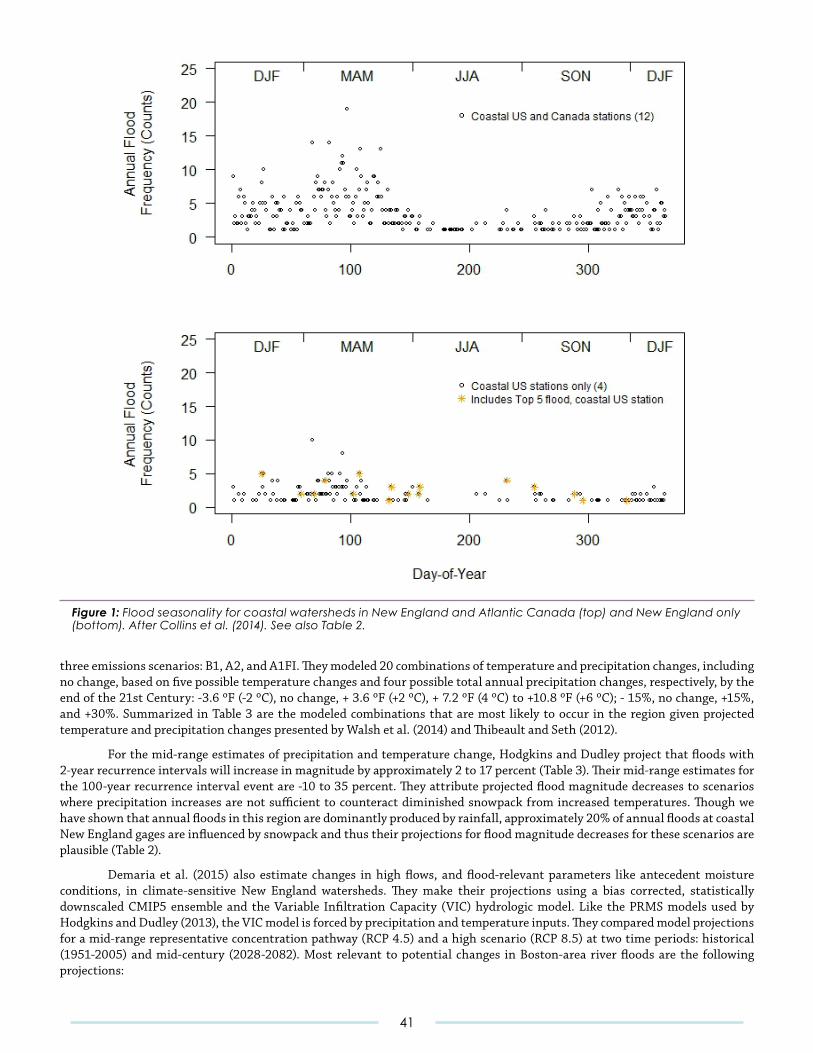
three emissions scenarios: B1, A2, and A1FI. They modeled 20 combinations of temperature and precipitation changes, including no change, based on five possible temperature changes and four possible total annual precipitation changes, respectively, by the end of the 21st Century: -3.6 ºF (-2 ºC), no change, + 3.6 ºF (+2 ºC), + 7.2 ºF (4 ºC) to +10.8 ºF (+6 ºC); - 15%, no change, +15%, and +30%. Summarized in Table 3 are the modeled combinations that are most likely to occur in the region given projected temperature and precipitation changes presented by Walsh et al. (2014) and Thibeault and Seth (2012).

For the mid-range estimates of precipitation and temperature change, Hodgkins and Dudley project that floods with 2-year recurrence intervals will increase in magnitude by approximately 2 to 17 percent (Table 3). Their mid-range estimates for the 100-year recurrence interval event are -10 to 35 percent. They attribute projected flood magnitude decreases to scenarios where precipitation increases are not sufficient to counteract diminished snowpack from increased temperatures. Though we have shown that annual floods in this region are dominantly produced by rainfall, approximately 20% of annual floods at coastal New England gages are influenced by snowpack and thus their projections for flood magnitude decreases for these scenarios are plausible (Table 2).

Demaria et al. (2015) also estimate changes in high flows, and flood-relevant parameters like antecedent moisture conditions, in climate-sensitive New England watersheds. They make their projections using a bias corrected, statistically downscaled CMIP5 ensemble and the Variable Infiltration Capacity (VIC) hydrologic model. Like the PRMS models used by Hodgkins and Dudley (2013), the VIC model is forced by precipitation and temperature inputs. They compared model projections for a mid-range representative concentration pathway (RCP 4.5) and a high scenario (RCP 8.5) at two time periods: historical (1951-2005) and mid-century (2028-2082). Most relevant to potential changes in Boston-area river floods are the following projections:

Figure 1:FloodseasonalityforcoastalwatershedsinNewEnglandandAtlanticCanada(top)andNewEnglandonly(bottom).AfterCollinsetal.(2014).SeealsoTable2.

41

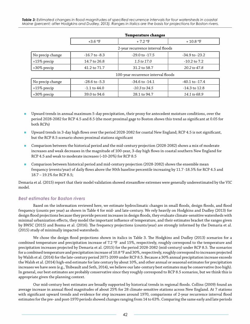
■ Upward trends in annual maximum 5-day precipitation, their proxy for antecedent moisture conditions, over the period 2028-2082 for RCP 4.5 and 8.5 (the most proximal gage to Boston shows this trend as significant at 0.05 for both RCPs)

■ Upward trends in 3-day high flows over the period 2028-2082 for coastal New England; RCP 4.5 is not significant, but the RCP 8.5 scenario shows proximal stations significant

■ Comparison between the historical period and the mid-century projection (2028-2082) shows a mix of moderate increases and weak decreases in the magnitude of 100-year, 3-day high flows in coastal southern New England for RCP 4.5 and weak to moderate increases (~10-20%) for RCP 8.5

■ Comparison between historical period and mid-century projection (2028-2082) shows the ensemble mean frequency (events/year) of daily flows above the 90th baseline percentile increasing by 11.7 -18.5% for RCP 4.5 and 18.7 – 19.1% for RCP 8.5;

Demaria et al. (2015) report that their model validation showed streamflow extremes were generally underestimated by the VIC model.

Best estimates for Boston rivers Based on the information reviewed here, we estimate hydroclimatic changes in small floods, design floods, and flood frequency (counts per year) as shown in Table 4 for mid- and late-century. We rely heavily on Hodgkins and Dudley (2013) for design flood projections because they provide percent increases in design floods, they evaluate climate-sensitive watersheds with minimal urbanization effects, they model the important influence of temperature, and their estimates bracket the ranges given by BWSC (2015) and Bosma et al. (2016). The frequency projections (counts/year) are strongly informed by the Demaria et al. (2015) study of minimally impacted watersheds.

We chose the design flood projections shown in italics in Table 3. The Hodgkins and Dudley (2013) scenarios for a combined temperature and precipitation increase of 7.2 ºF and 15%, respectively, roughly correspond to the temperature and precipitation increases projected by Demaria et al. (2015) for the period 2028-2082 (mid-century) under RCP 8.5. The scenarios for a combined temperature and precipitation increase of 10.8 ºF and 30%, respectively, roughly correspond to increases projected by Walsh et al. (2014) for the late-century period 2071-2099 under RCP 8.5. Because a 30% annual precipitation increase exceeds the Walsh et al. (2014) high-end estimate for late century by about 10%, and other annual or seasonal estimates for precipitation increases we have seen (e.g., Thibeault and Seth, 2014), we believe our late-century best estimates may be conservative (too high). In general, our best estimates are probably conservative since they roughly correspond to RCP 8.5 scenarios, but we think this is appropriate given the planning context.

Our mid-century best estimates are broadly supported by historical trends in regional floods. Collins (2009) found an average increase in annual flood magnitudes of about 25% for 28 climate-sensitive stations across New England. At 7 stations with significant upward trends and evidence for step increases around 1970, comparisons of 2-year recurrence interval flood estimates for the pre- and post-1970 periods showed changes ranging from 14 to 63%. Comparing the same early and late periods

Temperature changes

+3.6 ºF + 7.2 ºF + 10.8 ºF

2-year recurrence interval floods

No precip change -16.7 to -8.3 -29.0 to -17.5 -34.9 to -23.2

+15% precip 14.7 to 26.8 1.5 to 17.0 -10.2 to 7.2

+30% precip 41.2 to 71.7 31.2 to 58.7 20.2 to 47.8

100-year recurrence interval floods

No precip change -28.6 to -5.3 -34.6 to -14.1 -40.1 to -17.4

+15% precip -1.1 to 44.0 -10.3 to 34.5 -14.3 to 12.8

+30% precip 39.0 to 94.6 28.1 to 94.7 14.1 to 68.9

Table 3: EstimatedchangesinfloodmagnitudesofspecifiedrecurrenceintervalsforfourwatershedsincoastalMaine(percent;afterHodgkinsandDudley,2013).RangesinitalicsarethebasisforprojectionsforBostonrivers.

42

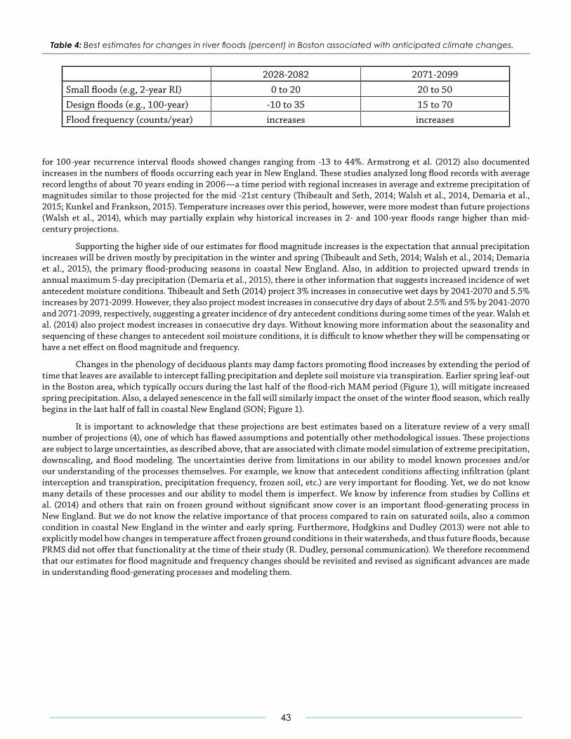
for 100-year recurrence interval floods showed changes ranging from -13 to 44%. Armstrong et al. (2012) also documented increases in the numbers of floods occurring each year in New England. These studies analyzed long flood records with average record lengths of about 70 years ending in 2006—a time period with regional increases in average and extreme precipitation of magnitudes similar to those projected for the mid -21st century (Thibeault and Seth, 2014; Walsh et al., 2014, Demaria et al., 2015; Kunkel and Frankson, 2015). Temperature increases over this period, however, were more modest than future projections (Walsh et al., 2014), which may partially explain why historical increases in 2- and 100-year floods range higher than mid-century projections.

Supporting the higher side of our estimates for flood magnitude increases is the expectation that annual precipitation increases will be driven mostly by precipitation in the winter and spring (Thibeault and Seth, 2014; Walsh et al., 2014; Demaria et al., 2015), the primary flood-producing seasons in coastal New England. Also, in addition to projected upward trends in annual maximum 5-day precipitation (Demaria et al., 2015), there is other information that suggests increased incidence of wet antecedent moisture conditions. Thibeault and Seth (2014) project 3% increases in consecutive wet days by 2041-2070 and 5.5% increases by 2071-2099. However, they also project modest increases in consecutive dry days of about 2.5% and 5% by 2041-2070 and 2071-2099, respectively, suggesting a greater incidence of dry antecedent conditions during some times of the year. Walsh et al. (2014) also project modest increases in consecutive dry days. Without knowing more information about the seasonality and sequencing of these changes to antecedent soil moisture conditions, it is difficult to know whether they will be compensating or have a net effect on flood magnitude and frequency.

Changes in the phenology of deciduous plants may damp factors promoting flood increases by extending the period of time that leaves are available to intercept falling precipitation and deplete soil moisture via transpiration. Earlier spring leaf-out in the Boston area, which typically occurs during the last half of the flood-rich MAM period (Figure 1), will mitigate increased spring precipitation. Also, a delayed senescence in the fall will similarly impact the onset of the winter flood season, which really begins in the last half of fall in coastal New England (SON; Figure 1).

It is important to acknowledge that these projections are best estimates based on a literature review of a very small number of projections (4), one of which has flawed assumptions and potentially other methodological issues. These projections are subject to large uncertainties, as described above, that are associated with climate model simulation of extreme precipitation, downscaling, and flood modeling. The uncertainties derive from limitations in our ability to model known processes and/or our understanding of the processes themselves. For example, we know that antecedent conditions affecting infiltration (plant interception and transpiration, precipitation frequency, frozen soil, etc.) are very important for flooding. Yet, we do not know many details of these processes and our ability to model them is imperfect. We know by inference from studies by Collins et al. (2014) and others that rain on frozen ground without significant snow cover is an important flood-generating process in New England. But we do not know the relative importance of that process compared to rain on saturated soils, also a common condition in coastal New England in the winter and early spring. Furthermore, Hodgkins and Dudley (2013) were not able to explicitly model how changes in temperature affect frozen ground conditions in their watersheds, and thus future floods, because PRMS did not offer that functionality at the time of their study (R. Dudley, personal communication). We therefore recommend that our estimates for flood magnitude and frequency changes should be revisited and revised as significant advances are made in understanding flood-generating processes and modeling them.

2028-2082 2071-2099Small floods (e.g, 2-year RI) 0 to 20 20 to 50Design floods (e.g., 100-year) -10 to 35 15 to 70Flood frequency (counts/year) increases increases

Table 4:Bestestimatesforchangesinriverfloods(percent)inBostonassociatedwithanticipatedclimatechanges.

43

F. References

Introduction:

Boston Water and Sewer Commission. (2015, June). Comprehensive-Integrated Sustainable Wastewater and Storm Drainage System Facilities Plan Final Report.

Callander, B.A., Varney, S.K. (eds) Climate change 1992. The Supplementary Report to the IPCC Scientific Assessment. Cambridge University Press, Cambridge, pp 71–95.

Chapel, B. (2015). A ‘Scorcher’: 2015 Shatters Record As Warmest Year, NASA and NOAA Say. NPR. Retrieved from: http://www.npr.org/sections/thetwo-way/2016/01/20/463709775/a-scorcher-2015-shatters-record-as-warmest-year-nasa-and-noaa-say

City of Cambridge. (2015). Climate Change Vulnerability Assessment, Cambridge MA November 2015. Douglas, E., Kirschen, P., Vivien, L., Watson, C., & Wormser, J. (2013). The Boston Harbor Association.

Preparing for the Rising Tide.Inman, M. (2011). Opening the future. Nature Feature. Intergovernmental Panel on Climate Change (IPCC). (1990). First Assessment Report (FAR). Intergovernmental Panel on Climate Change (IPCC). (2001). Third Assessment Report (TAR). Intergovernmental Panel on Climate Change (IPCC). (2007). Fourth Assessment Report (AR4). Intergovernmental Panel on Climate Change (IPCC). (2013). Fifth Assessment Report (AR5). IPCC, 2000. Emissions Scenarios, Summary for Policymakers, Special Report of WG III, available online at

https://www.ipcc.ch/pdf/special-reports/spm/sres-en.pdfLeggett, J., Pepper, W., Swart, R.J. (1992) Emissions Scenarios for the IPCC: an Update. In: Houghton JT,

https://www.ipcc.ch/ipccreports/1992%20IPCC%20Supplement/IPCC_Suppl_Report_1992_wg_I/ipcc_wg_I_1992_suppl_report_section_a3.pdf

Masui, T., Matsumoto, K., Hijioka, Y., Kinoshita, T., Nozawa, T., Ishiwatari, Nakicenovic et al. (2000) Special Report on Emissions Scenarios (SRES). Cambridge University Press, Cambridge, available online at http://www.ipcc.ch/ipccreports/sres/emission/index.php?idp=0

Meinshausen, M., Smith, S.J., Calvin, K., Daniel, J.S, Kainuma, M.L.T., Lamarque, J.F, Matsumoto, K., Montzka, S.A., Raper, S.C.B., Riahi, K., Thomson, A., Velders, G.J.M., & van Vuuren, D.P.P. (2011). The RCP greenhouse gas concentrations and their extensions from 1765 and 2300. Climatic Change.

Melillo, J.M., T.T.C. Richmond, and G.W. Yohe, 2014. Climate Change Impacts in the United States: The Third National Climate Assessment. U.S. Global Change Research Program, Washington, D.C.

Nakicenovic, N., Alcamo, J., Davis, G., de Vries, B., Fenhann, J., Gaffin, S., Gregory, K., Grubler, A., Jung, T.Y., Kram, T., LaRovere, E.L., Michaelis, L., Mori, S., Morita, T., Pepper, W., Pitcher, H., Price, L., Raihi, P, Roehrl, A., Rogner, H, Sankoviski, A., Schesinger, M., Shukla, P, Smith, S., Swart, R., van Rooijen, S., Victor, N., & Dadi, Z. (2000). Emissions Scenarios. A Special Report of Working Group III of the Intergovernmental Panel on Climate Change.

National Oceanic and Atmospheric Administration. (2015a). Global Analysis-Annual 2015. National Centers for Environmental Information. Retrieved from: https://www.ncdc.noaa.gov/sotc/global/201513

National Oceanic and Atmospheric Administration (NOAA). (2015b). How Reliable Are the Models Used to Make Projections of Future Climate Change? Frequently Asked Questions. 8.1. Retrieved from: http://oceanservice.noaa.gov/education/pd/climate/factsheets/howreliable.pdf

National Weather Service. (2015). NWS Weather Forecast Office-Boston/Taunton. National Oceanic and Atmospheric Administration. Retrieved from: http://www.weather.gov/Boston

Spector, C., & Bamberger, L. (2013). City of Boston. Greenovate Boston Climate Ready Boston: Municipal Vulnerability to Climate Change.

44

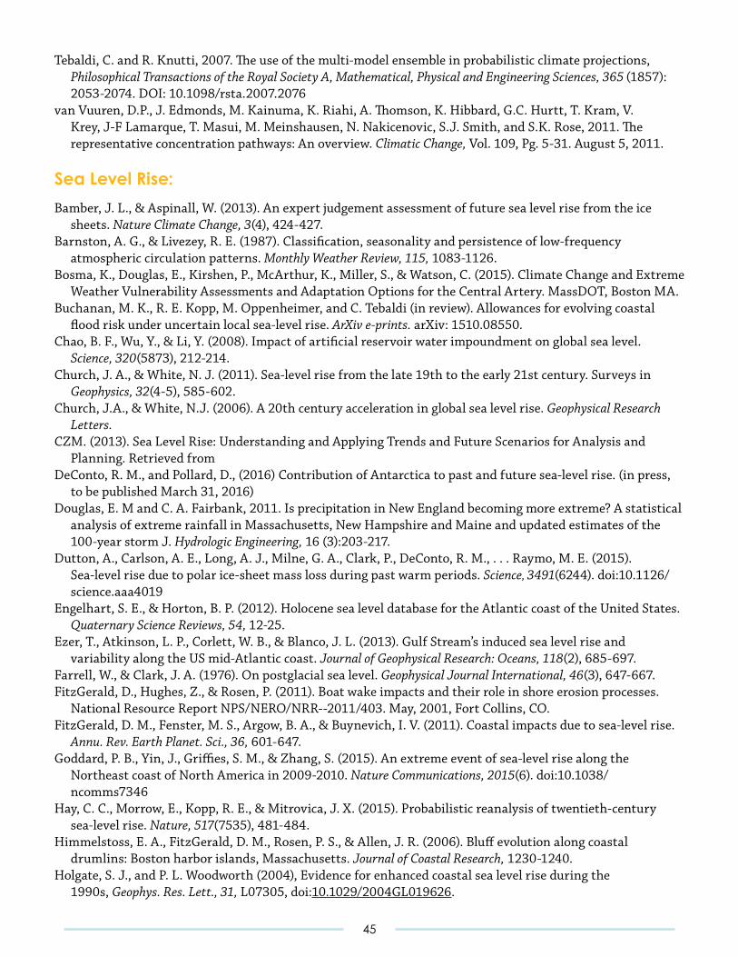
Tebaldi, C. and R. Knutti, 2007. The use of the multi-model ensemble in probabilistic climate projections, Philosophical Transactions of the Royal Society A, Mathematical, Physical and Engineering Sciences, 365 (1857): 2053-2074. DOI: 10.1098/rsta.2007.2076

van Vuuren, D.P., J. Edmonds, M. Kainuma, K. Riahi, A. Thomson, K. Hibbard, G.C. Hurtt, T. Kram, V. Krey, J-F Lamarque, T. Masui, M. Meinshausen, N. Nakicenovic, S.J. Smith, and S.K. Rose, 2011. The representative concentration pathways: An overview. Climatic Change, Vol. 109, Pg. 5-31. August 5, 2011.

Sea Level Rise:

Bamber, J. L., & Aspinall, W. (2013). An expert judgement assessment of future sea level rise from the ice sheets. Nature Climate Change, 3(4), 424-427.

Barnston, A. G., & Livezey, R. E. (1987). Classification, seasonality and persistence of low-frequency atmospheric circulation patterns. Monthly Weather Review, 115, 1083-1126.

Bosma, K., Douglas, E., Kirshen, P., McArthur, K., Miller, S., & Watson, C. (2015). Climate Change and Extreme Weather Vulnerability Assessments and Adaptation Options for the Central Artery. MassDOT, Boston MA.

Buchanan, M. K., R. E. Kopp, M. Oppenheimer, and C. Tebaldi (in review). Allowances for evolving coastal flood risk under uncertain local sea-level rise. ArXiv e-prints. arXiv: 1510.08550.

Chao, B. F., Wu, Y., & Li, Y. (2008). Impact of artificial reservoir water impoundment on global sea level. Science, 320(5873), 212-214.

Church, J. A., & White, N. J. (2011). Sea-level rise from the late 19th to the early 21st century. Surveys in Geophysics, 32(4-5), 585-602.

Church, J.A., & White, N.J. (2006). A 20th century acceleration in global sea level rise. Geophysical Research Letters.

CZM. (2013). Sea Level Rise: Understanding and Applying Trends and Future Scenarios for Analysis and Planning. Retrieved from

DeConto, R. M., and Pollard, D., (2016) Contribution of Antarctica to past and future sea-level rise. (in press, to be published March 31, 2016)

Douglas, E. M and C. A. Fairbank, 2011. Is precipitation in New England becoming more extreme? A statistical analysis of extreme rainfall in Massachusetts, New Hampshire and Maine and updated estimates of the 100-year storm J. Hydrologic Engineering, 16 (3):203-217.

Dutton, A., Carlson, A. E., Long, A. J., Milne, G. A., Clark, P., DeConto, R. M., . . . Raymo, M. E. (2015). Sea-level rise due to polar ice-sheet mass loss during past warm periods. Science, 3491(6244). doi:10.1126/science.aaa4019

Engelhart, S. E., & Horton, B. P. (2012). Holocene sea level database for the Atlantic coast of the United States. Quaternary Science Reviews, 54, 12-25.

Ezer, T., Atkinson, L. P., Corlett, W. B., & Blanco, J. L. (2013). Gulf Stream’s induced sea level rise and variability along the US mid-Atlantic coast. Journal of Geophysical Research: Oceans, 118(2), 685-697.

Farrell, W., & Clark, J. A. (1976). On postglacial sea level. Geophysical Journal International, 46(3), 647-667. FitzGerald, D., Hughes, Z., & Rosen, P. (2011). Boat wake impacts and their role in shore erosion processes.

National Resource Report NPS/NERO/NRR--2011/403. May, 2001, Fort Collins, CO. FitzGerald, D. M., Fenster, M. S., Argow, B. A., & Buynevich, I. V. (2011). Coastal impacts due to sea-level rise.

Annu. Rev. Earth Planet. Sci., 36, 601-647. Goddard, P. B., Yin, J., Griffies, S. M., & Zhang, S. (2015). An extreme event of sea-level rise along the

Northeast coast of North America in 2009-2010. Nature Communications, 2015(6). doi:10.1038/ncomms7346

Hay, C. C., Morrow, E., Kopp, R. E., & Mitrovica, J. X. (2015). Probabilistic reanalysis of twentieth-century sea-level rise. Nature, 517(7535), 481-484.

Himmelstoss, E. A., FitzGerald, D. M., Rosen, P. S., & Allen, J. R. (2006). Bluff evolution along coastal drumlins: Boston harbor islands, Massachusetts. Journal of Coastal Research, 1230-1240.

Holgate, S. J., and P. L. Woodworth (2004), Evidence for enhanced coastal sea level rise during the 1990s, Geophys. Res. Lett., 31, L07305, doi:10.1029/2004GL019626.

45

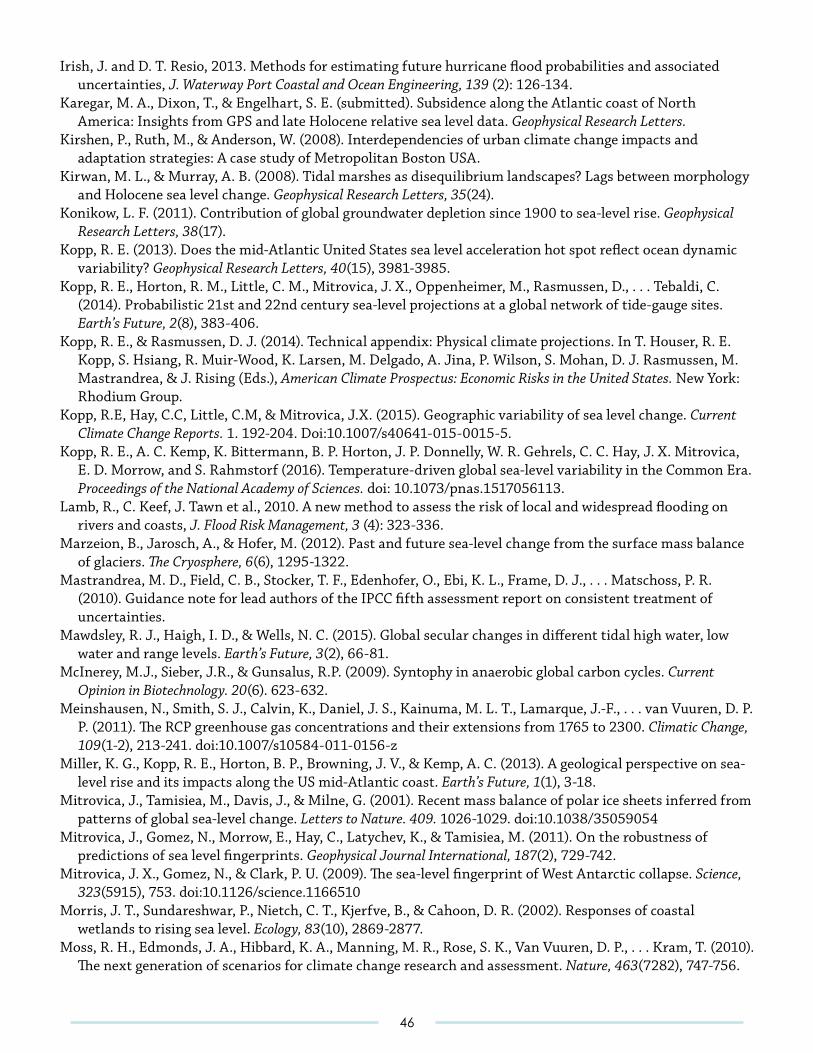
Irish, J. and D. T. Resio, 2013. Methods for estimating future hurricane flood probabilities and associated uncertainties, J. Waterway Port Coastal and Ocean Engineering, 139 (2): 126-134.

Karegar, M. A., Dixon, T., & Engelhart, S. E. (submitted). Subsidence along the Atlantic coast of North America: Insights from GPS and late Holocene relative sea level data. Geophysical Research Letters.

Kirshen, P., Ruth, M., & Anderson, W. (2008). Interdependencies of urban climate change impacts and adaptation strategies: A case study of Metropolitan Boston USA.

Kirwan, M. L., & Murray, A. B. (2008). Tidal marshes as disequilibrium landscapes? Lags between morphology and Holocene sea level change. Geophysical Research Letters, 35(24).

Konikow, L. F. (2011). Contribution of global groundwater depletion since 1900 to sea-level rise. Geophysical Research Letters, 38(17).

Kopp, R. E. (2013). Does the mid-Atlantic United States sea level acceleration hot spot reflect ocean dynamic variability? Geophysical Research Letters, 40(15), 3981-3985.

Kopp, R. E., Horton, R. M., Little, C. M., Mitrovica, J. X., Oppenheimer, M., Rasmussen, D., . . . Tebaldi, C. (2014). Probabilistic 21st and 22nd century sea-level projections at a global network of tide-gauge sites. Earth’s Future, 2(8), 383-406.

Kopp, R. E., & Rasmussen, D. J. (2014). Technical appendix: Physical climate projections. In T. Houser, R. E. Kopp, S. Hsiang, R. Muir-Wood, K. Larsen, M. Delgado, A. Jina, P. Wilson, S. Mohan, D. J. Rasmussen, M. Mastrandrea, & J. Rising (Eds.), American Climate Prospectus: Economic Risks in the United States. New York: Rhodium Group.

Kopp, R.E, Hay, C.C, Little, C.M, & Mitrovica, J.X. (2015). Geographic variability of sea level change. Current Climate Change Reports. 1. 192-204. Doi:10.1007/s40641-015-0015-5.

Kopp, R. E., A. C. Kemp, K. Bittermann, B. P. Horton, J. P. Donnelly, W. R. Gehrels, C. C. Hay, J. X. Mitrovica, E. D. Morrow, and S. Rahmstorf (2016). Temperature-driven global sea-level variability in the Common Era. Proceedings of the National Academy of Sciences. doi: 10.1073/pnas.1517056113.

Lamb, R., C. Keef, J. Tawn et al., 2010. A new method to assess the risk of local and widespread flooding on rivers and coasts, J. Flood Risk Management, 3 (4): 323-336.

Marzeion, B., Jarosch, A., & Hofer, M. (2012). Past and future sea-level change from the surface mass balance of glaciers. The Cryosphere, 6(6), 1295-1322.

Mastrandrea, M. D., Field, C. B., Stocker, T. F., Edenhofer, O., Ebi, K. L., Frame, D. J., . . . Matschoss, P. R. (2010). Guidance note for lead authors of the IPCC fifth assessment report on consistent treatment of uncertainties.

Mawdsley, R. J., Haigh, I. D., & Wells, N. C. (2015). Global secular changes in different tidal high water, low water and range levels. Earth’s Future, 3(2), 66-81.

McInerey, M.J., Sieber, J.R., & Gunsalus, R.P. (2009). Syntophy in anaerobic global carbon cycles. Current Opinion in Biotechnology. 20(6). 623-632.

Meinshausen, N., Smith, S. J., Calvin, K., Daniel, J. S., Kainuma, M. L. T., Lamarque, J.-F., . . . van Vuuren, D. P. P. (2011). The RCP greenhouse gas concentrations and their extensions from 1765 to 2300. Climatic Change, 109(1-2), 213-241. doi:10.1007/s10584-011-0156-z

Miller, K. G., Kopp, R. E., Horton, B. P., Browning, J. V., & Kemp, A. C. (2013). A geological perspective on sea-level rise and its impacts along the US mid-Atlantic coast. Earth’s Future, 1(1), 3-18.

Mitrovica, J., Tamisiea, M., Davis, J., & Milne, G. (2001). Recent mass balance of polar ice sheets inferred from patterns of global sea-level change. Letters to Nature. 409. 1026-1029. doi:10.1038/35059054

Mitrovica, J., Gomez, N., Morrow, E., Hay, C., Latychev, K., & Tamisiea, M. (2011). On the robustness of predictions of sea level fingerprints. Geophysical Journal International, 187(2), 729-742.

Mitrovica, J. X., Gomez, N., & Clark, P. U. (2009). The sea-level fingerprint of West Antarctic collapse. Science, 323(5915), 753. doi:10.1126/science.1166510

Morris, J. T., Sundareshwar, P., Nietch, C. T., Kjerfve, B., & Cahoon, D. R. (2002). Responses of coastal wetlands to rising sea level. Ecology, 83(10), 2869-2877.

Moss, R. H., Edmonds, J. A., Hibbard, K. A., Manning, M. R., Rose, S. K., Van Vuuren, D. P., . . . Kram, T. (2010). The next generation of scenarios for climate change research and assessment. Nature, 463(7282), 747-756.

46

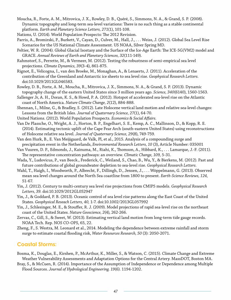
Moucha, R., Forte, A. M., Mitrovica, J. X., Rowley, D. B., Quéré, S., Simmons, N. A., & Grand, S. P. (2008). Dynamic topography and long-term sea-level variations: There is no such thing as a stable continental platform. Earth and Planetary Science Letters, 271(1), 101-108.

Nations, U. (2014). World Population Prospects: The 2012 Revision.Parris, A., Bromirski, P., Burkett, V., Cayan, D., Culver, M., Hall, J., . . . Weiss, J. (2012). Global Sea Level Rise

Scenarios for the US National Climate Assessment. US NOAA, Silver Spring MD. Peltier, W. R. (2004). Global Glacial Isostasy and the Surface of the Ice-Age Earth: The ICE-5G(VM2) model and

GRACE. Annual Reviews of Earth and Planetary Sciences, 32(111-149). Rahmstorf, S., Perrette, M., & Vermeer, M. (2012). Testing the robustness of semi-empirical sea level

projections. Climate Dynamics, 39(3-4), 861-875. Rignot, E., Velicogna, I., van den Broeke, M., Monaghan, A., & Lenaerts, J. (2011). Acceleration of the

contribution of the Greenland and Antarctic ice sheets to sea level rise. Geophysical Research Letters. doi:10.1029/2011GL046583.

Rowley, D. B., Forte, A. M., Moucha, R., Mitrovica, J. X., Simmons, N. A., & Grand, S. P. (2013). Dynamic topography change of the eastern United States since 3 million years ago. Science, 340(6140), 1560-1563.

Sallenger Jr, A. H., Doran, K. S., & Howd, P. A. (2012). Hotspot of accelerated sea-level rise on the Atlantic coast of North America. Nature Climate Change, 2(12), 884-888.

Shennan, I., Milne, G., & Bradley, S. (2012). Late Holocene vertical land motion and relative sea-level changes: Lessons from the British Isles. Journal of Quaternary Science, 27(1), 64-70.

United Nations. (2012). World Population Prospects. Economics & Social Affairs. Van De Plassche, O., Wright, A. J., Horton, B. P., Engelhart, S. E., Kemp, A. C., Mallinson, D., & Kopp, R. E.

(2014). Estimating tectonic uplift of the Cape Fear Arch (south-eastern United States) using reconstructions of Holocene relative sea level. Journal of Quaternary Science, 29(8), 749-759.

Van den Hurk, B., E. Van Meijigaard, de Valk, Pl, et al., 2015. Analysis of a compounding surge and precipitation event in the Netherlands, Environmental Research Letters, 10 (3), Article Number: 035001

Van Vuuren, D. P., Edmonds, J., Kainuma, M., Riahi, K., Thomson, A., Hibbard, K., . . . Lamarque, J.-F. (2011). The representative concentration pathways: an overview. Climatic Change, 109, 5-31.

Wada, Y., Ludovicus, P., van Beeck., Frederick, C., Weiland, S., Chao, B., Wu, Y., & Bierkens, M. (2012). Past and future contributions of global groundwater depletion to sea-level rise. Geophysical Research Letters.

Wahl, T., Haigh, I., Woodworth, P., Albrecht, F., Dillingh, D., Jensen, J., . . . Wöppelmann, G. (2013). Observed mean sea level changes around the North Sea coastline from 1800 to present. Earth-Science Reviews, 124, 51-67.

Yin, J. (2012). Century to multi-century sea level rise projections from CMIP5 models. Geophysical Research Letters, 39. doi:10.1029/2012GL052947

Yin, J., & Goddard, P. B. (2013). Oceanic control of sea level rise patterns along the East Coast of the United States. Geophysical Reseach Letters, 40, 1-7. doi:10.1002/2013GL057992

Yin, J., Schlesinger, M. E., & Stouffer, R. J. (2009). Model projections of rapid sea-level rise on the northeast coast of the United States. Nature Geoscience, 2(4), 262-266.

Zervas, C., Gill, S., & Sweet, W. (2013). Estimating vertical land motion from long-term tide gauge records. NOAA Tech. Rep. NOS CO-OPS, 65, 22.

Zheng, F., S. Westra, M. Leonard et al., 2014. Modeling the dependence between extreme rainfall and storm surge to estimate coastal flooding risk, Water Resources Research, 50 (3): 2050-2071.

Coastal Storms:

Bosma, K., Douglas, E., Kirshen, P., McArthur, K., Miller, S., & Watson, C. (2015). Climate Change and Extreme Weather Vulnerability Assessments and Adaptation Options for the Central Artery. MassDOT, Boston MA.

Bray, S., & McCuen, R. (2014). Importance of the Assumption of Independence or Dependence among Multiple Flood Sources. Journal of Hydrological Engineering. 19(6). 1194-1202.

47

Buchanan, M.K., R.E. Kopp, M. Oppenheimer, and Tebaldi, C. (2016) Allowances for evolving coastal flood risk under uncertain local sea-level rise. arXiv preprint arXiv:1510.08550.

BWSC (Boston Water and Sewer Commission) Final Task Force Report (2015): Section 7 Climate ChangeCOBHMP (City of Boston Natural Hazard Mitigation Plan) Revised Draft (2015): A Component Plan of Boston’s

Comprehensive Emergency Management ProgramColle, B.A. et al. (2013): Historical evaluation and future prediction of eastern North American and western Atlantic

extratropical cyclones in the CMIP5 models during the cool season, J. Climate, DOI: 10.1175/JCLI-D-12-00498.1Douglas, E. M and C. A. Fairbank, 2011. Is precipitation in New England becoming more extreme? A statistical

analysis of extreme rainfall in Massachusetts, New Hampshire and Maine and updated estimates of the 100-year storm J. Hydrologic Engineering, 16 (3), 203-217.

Emanuel, K (2013) Downscaling CMIP5 climate models shows increased tropical cyclone activity over the 21st century. PNAS, doi/10.1073/pnas.1301293110.

Holgate, S., & Woodworth, P. (2004). Evidence for enhanced coastal sea level rise during the 1990s. Oceans. 31(7). DOI:10.1029/2004GL019626

Hunter, J. (2011). A simple technique for estimating an allowance for uncertain sea-level rise. Climatic Change. 113(2). 239-252.

Intergovernmental Panel on Climate Change (IPCC). (2013). Fifth Assessment Report. Kirshen, P., Ruth, M., & Anderson, W. (2008). Interdependencies of urban climate change impacts and

adaptation strategies: a case study of Metropolitan Boston USA. Lamb, R., Keef, C., Tawn, J., Laeger, S., Meadowcroft, I., Surendran, S., Dunning, P., &

Batstone, C. (2010). A new method to assess the risk of local and widespread flooding on rivers and coasts. Journal of Flood Risk Management. 3(4). 323-336.

MassCCAR (Massachusetts Climate Change Adaptation Report) (2011)NECIA (Northeast Climate Impacts Assessment) Report (2007): Confronting Climate Change in the U.S.

Northeast: Science, Impacts, and SolutionsNHCRHC (New Hampshire Coastal Risks and Hazards Commission) Report (2014) Sea-level Rise, Storm Surges,

and Extreme Precipitation in Coastal New Hampshire: Analysis of Past and Projected Future Trends.Orton, P., S. Vinogradov, N. Georgas, A. Blumberg, N. Lin, V. Gornitz, C. Little, K. Jacob, and R. Horton (2015),

New York City Panel on Climate Change 2015 report chapter 4: Dynamic coastal flood modeling, Ann. N. Y. Acad. Sci., 1336(1), 56‐66.

Patrick, L., W. Solecki, K. H. Jacob, H. Kunreuther, and G. Nordenson (2015), New York City Panel on Climate Change 2015 Report Chapter 3: Static Coastal Flood Mapping, Ann. N. Y. Acad. Sci., 1336(1), 45‐55.

Resio, D, Irish, J., Westerink, J., & Powell, N. (2012). The effect of uncertainty on estimates of hurricane surge hazards. Natural Hazards. 66(3). 1443-1459.

Seller, C. and F.W. Zwiers (2015): How will climate change affect explosive cyclones in the extratropics of the Northern Hemisphere? Clim. Dyn., DOI 10.1007/s00382-015-2791-y

Stedinger, J.R., R.M. Vogel and E. Foufoula-Georgiou, Frequency Analysis of Extreme Events, Chapter 18, Handbook of Hydrology, McGraw-Hill Book Company, David R. Maidment, Editor-in-Chief, 1993.

TBHA (The Boston Harbor Association) Report (2013): Preparing for a Rising Tide.Van den Hurk, B., E. Van Meijigaard, de Valk, Pl, et al., 2015. Analysis of a compounding surge and

precipitation event in the Netherlands, Environmental Research Letters, 10 (3), Article Number: 035001Vogel, R.M. and J.R. Stedinger (1984), Floodplain Delineation in Ice Jam Prone Regions, Journal of Water

Resources Planning and Management, 110(2), 206-219.Wahl, T. (2015). Statistical Assessment of Storm Surge Scenarios Within Integrated Risk Analyses. Coastal

Engineering Journal. 57(1). DOI: 10.1142/S0578563415400033.Xu, J., Chen, Z., Tiang, J. & Su, S. (2014). T-Storm: Traffic-Aware Online Scheduling in Storm. Zheng, F., S. Westra, M. Leonard et al., 2014. Modeling the dependence between extreme rainfall and storm

surge to estimate coastal flooding risk, Water Resources Research, 50 (3): 2050-2071.

48

Extreme Precipitation:

Armstrong, W.H., Collins, M.J., and Snyder, N.P., 2012. Increased frequency of low magnitude floods in New England. Journal of the American Water Resources Association (JAWRA) 48(2):306-320, doi: 10.1111 ⁄ j.1752-1688.2011.00613.x

Barlow, M.A. (2012). The Madden-Julian oscillation influence on Africa and west Asia. Interseasonal Variability in the Coupled Tropical Ocean-Atmosphere System.

Barnes, E. A. (2013). Revisiting the evidence linking Arctic amplification to extreme weather in midlatitudes. Geophysical Research Letters, 40(17), 4734-4739.

Bosma, K., Douglas, E., Kirshen, P., McArthur, K., Miller, S., Watson, C., 2016. MassDOT-FHWA Pilot Project Report: Climate Change and Extreme Weather Vulnerability Assessments and Adaptation Options for the Central Artery.

Boston Water and Sewer Commission (BWSC), 2015. Comprehensive-Integrated Sustainable Wastewater and Storm Drainage System Facilities Plan Final Report. Retrieved from: DVD of the Report.

City of Cambridge. (2015). Climate Change Vulnerability Assessment, Cambridge MA November 2015.

Cohen, J., M. Barlow, and K. Saito, 2009: Decadal Fluctuations in Planetary Wave Forcing Modulate Global Warming in Late Boreal Winter. J. Climate, 22, 4418–4426.

Cohen, J., J. Furtado, M. Barlow, V. Alexeev, J. Cherry, 2012: Asymmetric seasonal temperature trends. Geophys. Res. Lett., 39, L04705.

Cohen, J., J.A. Screen, J.C. Furtado, M. Barlow, D. Whittleston, D. Coumou, J. Francis, K. Dethloff, D. Entekhabi, J. Overland & J. Jones, 2014: Recent Arctic amplification and extreme mid-latitude weather, Nature Geosci., 7, 627-637.

Colle, B.A, Zhang, Z., Lombardo, K., Chang, E., Liu, P., & Zhang, M. (2013). Historical evaluation and future prediction of eastern North American and western Atlantic extratropical cyclones in the CMIP5 models during the cool season. Journal of Climate, 26, 6882-6903.

Colle, B. A., J. F. Booth, & E. K. M. Chang. (2015) A Review of Historical and Future Changes of Extratropical Cyclones and Associated Impacts Along the US East Coast. Current Climate Change Reports 1, 125-143.

Collins, M.J., 2009. Evidence for changing flood risk in New England since the late 20th century. Journal of the American Water Resources Association (JAWRA) 45(2):279-290, doi: 10.1111/j.1752-1688.2008.00277.x

Collins, M.J., Kirk, J.P., Pettit, J., DeGaetano, A.T., McCown, M.S., Peterson, T.C., Means, T.N., and Zhang, X., 2014. Annual floods in New England (USA) and Atlantic Canada: Synoptic climatology and generating mechanisms. Physical Geography, 35(3), 195-219, doi:10.1080/02723646.2014.888510

DeAngelis, A., Broccoli, A., & Decker, S. (2013). A Comparison of CMIP# Simulations of Precipitation over North America with Observations: Daily Statistics and Circulation Features Accompanying Extreme Events. DOI: http://dx.doi.org/10.1175/JCLI-D-12-00374.1h

DeGaetano, A., 2009. Time-Dependent Changes in Extreme-Precipitation Return-Period Amounts in the Continental United States. J. Appl. Meteor. Climatol., 48, 2086–2099.

Demaria, E.M., Palmer, R.N., and Roundy, J.K., 2015. Regional climate change projections of streamflow characteristics in the Northeast and Midwest US. Journal of Hydrology: Regional Studies, doi:10.1016/j.ejrh.2015.11.007

Deser, C., Phillips, A. S., Alexander, M. A., & Smoliak, B. V. (2014). Projecting North American climate over the next 50 years: Uncertainty due to internal variability. Journal of Climate, 27(6), 2271-2296.

Deser, C., A. S. Phillips, V. Bourdette, and H. Teng, 2012b: Uncertainty in climate change projections: The role of internal variability. Climate Dyn., 38, 527–546, doi:10.1007/s00382-010-0977-x.

Douglas, E. M and C. A. Fairbank, 2011. Is precipitation in New England becoming more extreme? A statistical analysis of extreme rainfall in Massachusetts, New Hampshire and Maine and updated estimates of the 100-year storm J. Hydrologic Engineering, 16 (3):203-217.

Fischer, E. M. & Knutti, R. Heated debate on cold weather. Nature Clim. Change 4, 537–538(2014).Francis, J. A. & Vavrus, S. J. Evidence linking Arctic amplification to extreme weather in mid-latitudes.

Geophys. Res. Lett. 39, L06801 (2012).

49

Francis, J. A. & Vavrus, S. J. Evidence for a wavier jet stream in response to rapid Arctic warming. Environ. Res. Lett. 10, 014005 (2015).

Georgakakos, A., Fleming, P., Dettinger, M., Peters-Lidard, C., T.C., Richmond, Reckhow, K., White, K., & Yates, D. (2014). Water resources, in Climate Change Impacts in the United States: The Third National Climate Assessment. Global Change Res. Program, Washington, D.C.

Groisman, P. Y., R. W. Knight and T. R. Karl. (2012) Changes in Intense Precipitation over the Central United States, J. Hydrometeorology, 13: 47-66.

Guilbert, J., Betts, A. K., Rizzo, D. M., Beckage, B., & Bomblies, A. (2015). Characterization of increased persistence and intensity of precipitation in the northeastern United States. Geophysical Research Letters, 42(6), 1888-1893.

Hayhoe, K., Wake, C., Huntington, T., Luo, L., Schwartz, M., Sheffield, J., Wood., Anderson, B., Bradbury, J., DeGaetano, A., Troy, T., & Wolfe, D. (2007). Past and future changes in climate and hydrological indicators in the US Northeast. Climate Dynamics. 28(4). 381-407.

Hodgkins, G.A., and Dudley, R.W., 2013. Modeled future peak streamflows in four coastal Maine rivers. US Geological Survey Scientific Investigations Report, 5080, 18 pp.

Horton, R., G. Yohe, W. Easterling, R. Kates, M. Ruth, E. Sussman, A. Whelchel, D. Wolfe, and F. Lipschultz, 2014: Ch. 16: Northeast. Climate Change Impacts in the United States: The Third National Climate Assessment, J. M. Melillo, Terese (T.C.) Richmond, and G. W. Yohe, Eds., U.S. Global Change Research Program, 371-395. doi:10.7930/J0SF2T3P.

Huntington, T. G., Hodgkins, G. A., Keim, B. D., & Dudley, R. W. (2004). Changes in the proportion of precipitation occurring as snow in New England (1949-2000). Journal of Climate, 17(13), 2626-2636.

Klima, K., & Morgan, M. G. (2015). Ice storm frequencies in a warmer climate. Climatic Change, 133(2), 209-222.

Kug, J. S., Jeong, J. H., Jang, Y. S., Kim, B. M., Folland, C. K., Min, S. K., & Son, S. W. (2015). Two distinct influences of Arctic warming on cold winters over North America and East Asia. Nature Geoscience.

Kunkel, K.E., and Frankson, R.M., 2015. Global Land Surface Extremes of Precipitation: Data Limitations and Trends. Journal of Extreme Events, doi: 10.1142/S2345737615500049.

Lenton, T. M. (2011). Early warning of climate tipping points. Nature Climate Change, 1(4), 201-209.Liu, J., Curry, J. A., Wang, H., Song, M. & Horton, R. M. Impact of declining Arctic sea ice on winter snowfall.

Proc. Natl Acad. Sci. USA 109, 4074–4079 (2012).Lombardo, K., B. A. Colle, and Z. Zhang, 2015: Evaluation of Historical and Future Cool Season Precipitation

over the Eastern United States and Western Atlantic Storm Track Using CMIP5 Models. J. Climate, 28(2), 451-467. doi:10.1175/JCLI-D-14-00343.1

Maloney, E. D., Camargo, S. J., Chang, E., Colle, B., Fu, R., Geil, K. L., ... & Kinter, J. (2014). North American climate in CMIP5 experiments: Part iii: Assessment of twenty-first-century projections. Journal of Climate, 27(6), 2230-2270.

Ning, L., Riddle, E.E., & Bradley, R.S. (2015). Projected Changes in Climate Extremes over the Northeastern United States. Journal of Climate.

Notaro, M., Lorenz, D., Hoving, C., & Schummer, M. (2014). Twenty-First-Century Projections of Snowfall and Winter Severity across Central-Eastern North America. Journal of Climate, 27(17), 6526-6550.

O’Gorman, P. A. (2014). Contrasting responses of mean and extreme snowfall to climate change. Nature, 512(7515), 416-418.

Peterson, T., Heim, R., Hirsch, R., Kaiser, D., Brooks, H., Diffenbaugh, N., Dole, R., Giovannettone, J., Guirguis, K., Karl, T., Katz, R., Kunkel, K., Lettenmaier, D., McCabe, G., Paciorek, C., Ryber, K., Schubert, S., Silva, V., et al. (2013). Monitoring and Understanding Changes in Heat Waves, Cold Waves, Floods and Droughts in the United States: State of Knowledge. American Meterological Society.

Screen, J. A. & Simmonds, I. Exploring links between Arctic amplification and mid-latitude weather. Geophys. Res. Lett. 40, 959–964 (2013).

Screen, J. A. & Simmonds, I. Amplified mid-latitude planetary waves favour particular regional weather extremes. Nature Clim. Change 4, 704–709 (2014).

50

Screen, J. A., Deser, C., Simmonds, I. & Tomas, R. Atmospheric impacts of Arctic sea-ice loss, 1979–2009: Separating forced change from atmospheric internal variability. Clim. Dynam. 43, 333–344 (2013).

Serinaldi, F., and Kilsby, C.G., 2015. Stationarity is undead: Uncertainty dominates the distribution of extremes. Advances in Water Resources, 77, 17-36, doi:10.1016/j.advwatres.2014.12.013

Soden, B., & Held, I. (2006). An Assessment of Climate Feedbacks in Coupled Ocean-Atmosphere Models. American Meterological Society.

Stoner, A. M. K., K. Hayhoe, X. Yang and D. J. Wuebbles, 2012. An asynchronous regional regression model for statistical downscaling of daily climate variables, International Journal of Climatology, DOI: 10.1002/joc.3603.

Thibeault, J.M., and Seth, A., 2014. Changing climate extremes in the Northeast United States: Observations and projections from CMIP5. Climatic Change, 127(2), 273-287, doi:10. 1007/ s10584-014-1257-2

Thompson, D. W., Barnes, E. A., Deser, C., Foust, W. E., & Phillips, A. S. (2015). Quantifying the role of internal climate variability in future climate trends. Journal of Climate.

Vavrus, S. J., Notaro, M., & Lorenz, D. J. (2015). Interpreting climate model projections of extreme weather events. Weather and Climate Extremes, 10, 10-28.

Wallace, J. M., C. Deser, B. V. Smoliak, and A. S. Phillips, 2014: Attribution of climate change in the presence of internal variability. Climate Change: Multidecadal and Beyond, C. P. Chang et al., Eds., Asia-Pacific Weather and Climate Series, Vol. 6, World Scientific, in press.

Wallace, J. M., Held, I. M., Thompson, D. W., Trenberth, K. E. & Walsh, J. E. Global warming and winter weather. Science 343, 729–730 (2014).

Walsh, J., Wuebbles, D., Hayhoe, K., Kossin, J., Kunkel, K., Stephens, G., Thorne, P., Vose, R., Wehner, M., Willis, J., Anderson, D., Doney, S., Feely, R., Hennon, P., Kharin, V., Knutson, T., Landerer, F., Lenton, T., Kennedy, J., and Somerville, R., 2014. “Ch. 2: Our Changing Climate.” Climate Change Impacts in the United States: The Third National Climate Assessment, J. M. Melillo, Terese (T.C.) Richmond, and G. W. Yohe, Eds., U.S. Global Change Research Program, 19-67. doi:10.7930/J0KW5CXT.

Warrick, R., W. Ye, P. Kouwenhoven, J. E. Hay, C. Cheatham (2005). New developments of the SimCLIM model for simulating adaptation to risks arising from climate variability and change, In Zerger, A. and Argent, R.M. (eds) MODSIM 2005. International Congress on Modelling and Simulation, Modelling and Simulation Society of Australia and New Zealand.

Extreme Temperatures:

Adler, M., Harris, S., Krey, M., Plocinski, L., and Rebecchi, J. (2010). Preparing for Heat Waves in Boston: A Cool Way to Attack Global Warming. Prepared for City of Boston Environment Department & Tufts University Department of Urban and Environmental Policy and Planning. https://www.cityofboston.gov/images_documents/Preparing%20for%20Heat%20Waves%20in%20Boston_tcm3-31986.pdf

Akbari, H. (2005). Energy Saving Potentials and Air Quality Benefits of Urban Heat Island Mitigation. Lawrence Berkeley National Laboratory.

Amato, A. D., Ruth, M., Kirshen, P., & Horwitz, J. (2005). Regional energy demand responses to climate change: Methodology and application to the Commonwealth of Massachusetts. Climatic Change, 71(1-2), 175-201.

Barnett, A. G., Hajat, S., Gasparrini, A., & Rocklöv, J. (2012). Cold and heat waves in the United States. Environmental Research, 112, 218-224.

Blazejczyk, K., Epstein, Y., Jendritzky, G., Staiger, H., & Tinz, B. (2012). Comparison of UTCI to selected thermal indices. International Journal of Biometeorology, 56(3), 515-535.

Busch, C., et al. (2014). City of Boston Hazard Mitigation Plan. http://www.cityofboston.gov/environment/mitigationplan.asp.

Cash, D. et al. (2011). Massachusetts climate change adaptation report. Executive Office of Energy and Environmental Affairs and the Adaptation Advisory Committee, Boston.

51

Cherrier, J., Klein, Y., Link, H., Pillich, J., & Yonzan, N. (2016). Hybrid green infrastructure for reducing demands on urban water and energy systems: A New York City hypothetical case study. Journal of Environmental Studies and Sciences, 6(1), 77-89.

Coutts, E., Ito, K., Nardi, C., and Vuong, T. (2015). Planning Urban Heat Island Mitigation in Boston. Prepared for: The Trust for Public Land.

Dousset, B. et al. (2011). Satellite monitoring of summer heat waves in the Paris metropolitan area. International Journal of Climatology, 31(2), 313-323.

Faber, B., Daley, J., Elwell, H., Gochowski, K., & Robertson, B. (2014). Methodology for Mapping Urban Heat Island Isotherms. The Trust for Public Land’s Climate‐Smart Cities Program White Paper.

Faghmous, J. H., & Kumar, V. (2014). A Big Data Guide to Understanding Climate Change: The Case for Theory-Guided Data Science. Big Data, 2(3), 155-163.

Field, C. B. (Ed.). (2012). Managing the risks of extreme events and disasters to advance climate change adaptation: Special report of the intergovernmental panel on climate change. Cambridge University Press.

Frumhoff, P.C., J.J. McCarthy, J.M. Melillo, S.C. Moser, and D.J. Wuebbles. (2007). Confronting Climate Change in the U.S. Northeast: Science, Impacts, and Solutions. Synthesis report of the Northeast Climate Impacts Assessment (NECIA). Cambridge, MA: Union of Concerned Scientists (UCS).

Ganguly, A. R., Steinhaeuser, K., Erickson, D. J., Branstetter, M., Parish, E. S., Singh, N., ... & Buja, L. (2009). Higher trends but larger uncertainty and geographic variability in 21st century temperature and heat waves. Proceedings of the National Academy of Sciences, 106(37), 15555-15559.

Ganguly, A. R., Kodra, E. A., Agrawal, A., Banerjee, A., Boriah, S., Chatterjee, S., ... & Ganguli, P. (2014). Toward enhanced understanding and projections of climate extremes using physics-guided data mining techniques. Nonlinear Processes in Geophysics, 21(4), 777-795.

Ganguly, A. R., Kumar, D., Ganguli, P., Short, G., & Klausner, J. (2015). Climate Adaptation Informatics: Water Stress on Power Production. Computing in Science & Engineering, 17(6), 53-60.

Gleckler, P. J., Taylor, K. E., & Doutriaux, C. (2008). Performance metrics for climate models. Journal of Geophysical Research: Atmospheres (1984–2012), 113(D6).

Greene, S., Kalkstein, L. S., Mills, D. M., & Samenow, J. (2011). An examination of climate change on extreme heat events and climate-mortality relationships in large US cities. Weather, Climate, and Society, 3(4), 281-292.

Gutierrez, K., & LePrevost, C. (2016). Climate Justice in Rural Southeastern United States: A Review of Climate Change Impacts and Effects on Human Health. Int. J. Envion. Res. Public Health. 13(2). doi:10.3390/ijerph13020189

Hajat, S., Kovats, R. S., & Lachowycz, K. (2007). Heat-related and cold-related deaths in England and Wales: Who is at risk? Occupational and environmental medicine, 64(2), 93-100.

Hardin, A. W. (2015). Assessment of urban heat islands during hot weather in the US Northeast and linkages to microscale thermal and radiational properties (Doctoral dissertation, Texas Tech University).

Hayhoe, K., Wake, C. P., Huntington, T. G., Luo, L., Schwartz, M. D., Sheffield, J., ... & Troy, T. J. (2007). Past and future changes in climate and hydrological indicators in the US Northeast. Climate Dynamics, 28(4), 381-407.

Horton, R., G. Yohe, W. Easterling, R. Kates, M. Ruth, E. Sussman, A. Whelchel, D. Wolfe, and F. Lipschultz, 2014: Ch. 16: Northeast. Climate Change Impacts in the United States: The Third National Climate Assessment, J. M. Melillo, Terese (T.C.) Richmond, and G. W. Yohe, Eds., U.S. Global Change Research Program, 16-1-nn.

Houser, T., Hsiang, S., Kopp, R., & Larsen, K. (2015). Economic risks of climate change: An American prospectus. Columbia University Press.

Husser, A. (2016). Ontario’s Nipigon River bridge fails, severing Trans-Canada Highway. CBC News. http://www.cbc.ca/news/canada/thunder-bay/nipigon-river-bridge-closed-transcanada-1.3397831.

IPCC Fourth Assessment Report (AR4). (2007). The Physical Science Basis, 2, 580.Kharin, V. V., Zwiers, F. W., Zhang, X., & Wehner, M. (2013). Changes in temperature and precipitation

extremes in the CMIP5 ensemble. Climatic Change, 119(2), 345-357.

52

Kodra, E., Steinhaeuser, K., & Ganguly, A. R. (2011). Persisting cold extremes under 21st‐century warming scenarios. Geophysical Research Letters, 38(8).

Kodra, E., Ghosh, S., & Ganguly, A. R. (2012). Evaluation of global climate models for Indian monsoon climatology. Environmental Research Letters, 7(1), 014012.

Kodra, E., & Ganguly, A. R. (2014). Asymmetry of projected increases in extreme temperature distributions. Scientific Reports, 4.

Kumar, D., Kodra, E., & Ganguly, A. R. (2014). Regional and seasonal intercomparison of CMIP3 and CMIP5 climate model ensembles for temperature and precipitation. Climate Dynamics, 43(9-10), 2491-2518.

Meehl, G. A., & Tebaldi, C. (2004). More intense, more frequent, and longer lasting heat waves in the 21st century. Science, 305(5686), 994-997.

Melillo, J. M., Richmond, T. C., & Yohe, G. W. (2014). Climate change impacts in the United States: The third national climate assessment. US Global Change Research Program, 841.

Mishra, V., Ganguly, A. R., Nijssen, B., & Lettenmaier, D. P. (2015). Changes in observed climate extremes in global urban areas. Environmental Research Letters, 10(2), 024005.

Morris, J. T., Sundareshwar, P., Nietch, C. T., Kjerfve, B., & Cahoon, D. R. (2002). Responses of coastal wetlands to rising sea level. Ecology, 83(10), 2869-2877.

Muller, C. J., & O’Gorman, P. A. (2011). An energetic perspective on the regional response of precipitation to climate change. Nature Climate Change, 1(5), 266-271.

Murray, V., & Ebi, K. L. (2012). IPCC special report on managing the risks of extreme events and disasters to advance climate change adaptation (SREX). Journal of Epidemiology and Community Health, 66(9), 759-760.

National Climate Assessment. (2015). Climate Change Impacts in the United States. U.S. Global Change Research Program.

O’Gorman, P. A., & Schneider, T. (2009). The physical basis for increases in precipitation extremes in simulations of 21st-century climate change. Proceedings of the National Academy of Sciences, 106(35), 14773-14777.

Olivier, J. G. (2012). Trends in Global CO2 Emissions: 2012 Report (p. 40). Hague: PBL Netherlands Environmental Assessment Agency.

Pachauri, R. K., Allen, M. R., Barros, V. R., Broome, J., Cramer, W., Christ, R., ... & Dubash, N. K. (2014). Climate Change 2014: Synthesis Report. Contribution of Working Groups I, II and III to the Fifth Assessment Report of the Intergovernmental Panel on Climate Change.

Pall, P., Allen, M. R., & Stone, D. A. (2007). Testing the Clausius–Clapeyron constraint on changes in extreme precipitation under CO2 warming. Climate Dynamics, 28(4), 351-363.

Peterson, T. C., Heim Jr, R. R., Hirsch, R., Kaiser, D. P., Brooks, H., Diffenbaugh, N. S., ... & Katz, R. W. (2013). Monitoring and understanding changes in heat waves, cold waves, floods, and droughts in the United States: State of knowledge. Bulletin of the American Meteorological Society, 94(6), 821-834.

Petkova, E. P., Horton, R. M., Bader, D. A., & Kinney, P. L. (2013). Projected heat-related mortality in the US urban northeast. International Journal of Environmental Research and Public Health, 10(12), 6734-6747.

Petri, Y., & Caldeira, K. (2015). Impacts of global warming on residential heating and cooling degree-days in the United States. Scientific Reports, 5.

Rasmussen, D. J., Meinshausen, M. & Kopp, R. E. (in rev). Probability-weighted ensembles of U.S. county-level climate projections for climate risk analysis. ArXiv e-prints. arXiv: 1510.00313.

Saha, M., & Eckelman, M. J. (2014). Urban scale mapping of concrete degradation from projected climate change. Urban Climate, 9, 101-114.

Schlenker, W., & Roberts, M. J. (2009). Nonlinear temperature effects indicate severe damages to US crop yields under climate change. Proceedings of the National Academy of Sciences, 106(37), 15594-15598.

Sheridan, S. C. (2002). The redevelopment of a weather-type classification scheme for North America. International Journal of Climatology, 22(1), 51-68.

Stone, B., Vargo, J., & Habeeb, D. (2012). Managing climate change in cities: Will climate action plans work? Landscape and Urban Planning, 107(3), 263-271.

53

Stoner, A. M., Hayhoe, K., Yang, X., & Wuebbles, D. J. (2013). An asynchronous regional regression model for statistical downscaling of daily climate variables. International Journal of Climatology, 33(11), 2473-2494.

Stott, P. A., Gillett, N. P., Hegerl, G. C., Karoly, D. J., Stone, D. A., Zhang, X., & Zwiers, F. (2010). Detection and attribution of climate change: A regional perspective. Wiley Interdisciplinary Reviews: Climate Change, 1(2), 192-211.

Stott, P. A., et al. (2016). Attribution of extreme weather and climate‐related events. Wiley Interdisciplinary Reviews: Climate Change, 7(1), 23-41.

Street, M., Reinhart, C., Norford, L., Ochsendorf, J.: Urban heat island in Boston - An evaluation of urban air temperature models for predicting building energy use. In Proceedings of Building Simulation 2013: Chambery, France, 2013.

Sugiyama, M., Shiogama, H., & Emori, S. (2010). Precipitation extreme changes exceeding moisture content increases in MIROC and IPCC climate models. Proceedings of the National Academy of Sciences, 107(2), 571-575.

Vavrus, S. J., Notaro, M., & Lorenz, D. J. (2015). Interpreting climate model projections of extreme weather events. Weather and Climate Extremes, 10, 10-28.

Appendix A

Armstrong, W.H., Collins, M.J., and Snyder, N.P., 2012. Increased frequency of low magnitude floods in New England. Journal of the American Water Resources Association (JAWRA) 48(2):306-320, doi: 10.1111 ⁄ j.1752-1688.2011.00613.x

Bosma, K., Douglas, E., Kirshen, P., McArthur, K., Miller, S., Watson, C., 2016. MassDOT-FHWA Pilot Project Report: Climate Change and Extreme Weather Vulnerability Assessments and Adaptation Options for the Central Artery.

Boston Water and Sewer Commission (BWSC), 2015. Comprehensive-Integrated Sustainable Wastewater and Storm Drainage System Facilities Plan Final Report. Retrieved from: DVD of the Report.

Collins, M.J., 2009. Evidence for changing flood risk in New England since the late 20th century. Journal of the American Water Resources Association (JAWRA) 45(2):279-290, doi: 10.1111/j.1752-1688.2008.00277.x

Collins, M.J., Kirk, J.P., Pettit, J., DeGaetano, A.T., McCown, M.S., Peterson, T.C., Means, T.N., and Zhang, X., 2014. Annual floods in New England (USA) and Atlantic Canada: Synoptic climatology and generating mechanisms. Physical Geography, 35(3), 195-219, doi:10.1080/02723646.2014.888510

Demaria, E.M., Palmer, R.N., and Roundy, J.K., 2015. Regional climate change projections of streamflow characteristics in the Northeast and Midwest US. Journal of Hydrology: Regional Studies, doi:10.1016/j.ejrh.2015.11.007

Hodgkins, G.A., and Dudley, R.W., 2013. Modeled future peak streamflows in four coastal Maine rivers. US Geological Survey Scientific Investigations Report, 5080, 18 pp.

Kunkel, K.E., and Frankson, R.M., 2015. Global Land Surface Extremes of Precipitation: Data Limitations and Trends. Journal of Extreme Events, doi: 10.1142/S2345737615500049.

Thibeault, J.M., and Seth, A., 2014. Changing climate extremes in the Northeast United States: Observations and projections from CMIP5. Climatic Change, 127(2), 273-287, doi:10.1007/s10584-014-1257-2

Serinaldi, F., and Kilsby, C.G., 2015. Stationarity is undead: Uncertainty dominates the distribution of extremes. Advances in Water Resources, 77, 17-36, doi:10.1016/j.advwatres.2014.12.013

Walsh, J., Wuebbles, D., Hayhoe, K., Kossin, J., Kunkel, K., Stephens, G., Thorne, P., Vose, R., Wehner, M., Willis, J., Anderson, D., Doney, S., Feely, R., Hennon, P., Kharin, V., Knutson, T., Landerer, F., Lenton, T., Kennedy, J., and Somerville, R., 2014. “Ch. 2: Our Changing Climate”. Climate Change Impacts in the United States: The Third National Climate Assessment, J. M. Melillo, Terese (T.C.) Richmond, and G. W. Yohe, Eds., U.S. Global Change Research Program, 19-67. doi:10.7930/J0KW5CXT.

54

Climate Ready Boston is an initiative led by the City of Boston in partnership with the Green Ribbon Commission to develop resilient solutions which will prepare our city for climate change.

Resilient solutions for buildings, infrastructure, environmental systems, and residents will ensure Boston continues to prosper in the face of long-term climate uncertainties.

CLIMATEREADYBOSTON

City of BostonMayor Martin J. Walsh