Bone-Conducted Ultrasonic Hearing - Chalmers...
47
Bone-Conducted Ultrasonic Hearing: Can Distortion Product Otoacoustic Emissions Confirm Cochlear Involvement? Master’s Thesis in the Master’s programme in Sound and Vibration JENNIFER A. MARTIN Department of Civil and Environmental Engineering Division of Division of Applied Acoustics Room Acoustics Group CHALMERS UNIVERSITY OF TECHNOLOGY Göteborg, Sweden 2011 Master’s Thesis 2011:18
-
Upload
truongngoc -
Category
Documents
-
view
215 -
download
1
Transcript of Bone-Conducted Ultrasonic Hearing - Chalmers...

Bone-Conducted Ultrasonic Hearing:
Can Distortion Product Otoacoustic Emissions Confirm
Cochlear Involvement?
Master’s Thesis in the Master’s programme in Sound and Vibration
JENNIFER A. MARTIN
Department of Civil and Environmental Engineering
Division of Division of Applied Acoustics
Room Acoustics Group
CHALMERS UNIVERSITY OF TECHNOLOGY
Göteborg, Sweden 2011
Master’s Thesis 2011:18


MASTER’S THESIS 2011:18
Bone-Conducted Ultrasonic Hearing:
Can Distortion Product Otoacoustic Emissions Confirm Cochlear Involvement?
Master’s Thesis in the Master’s programme in Sound and Vibration
JENNIFER A. MARTIN
Department of Civil and Environmental Engineering
Division of Division of Applied Acoustics
Room Acoustics Group
CHALMERS UNIVERSITY OF TECHNOLOGY
Göteborg, Sweden 2011

Bone-Conducted Ultrasonic Hearing:
Can Distortion Product Otoacoustic Emissions Confirm Cochlear Involvement?
© JENNIFER A. MARTIN, 2011
Master’s Thesis 2011:18
Department of Civil and Environmental Engineering
Division of Applied Acoustics
Room Acoustics Group
Chalmers University of Technology
SE-412 96 Göteborg
Sweden
Telephone: + 46 (0)31-772 1000
Cover:
Left: Subject being tested during this study (see 5.2 Test Procedure),
Right: Photograph of cochlea
(http://www.bionicear-europe.com/en/hearing-loss/hearing-loss.html)
Chalmers Reproservice / Department of Civil and Environmental Engineering
Göteborg, Sweden 2011
I
Bone-Conducted Ultrasonic Hearing:
Can Distortion Product Otoacoustic Emissions Confirm Cochlear Involvement?
Master’s Thesis in the Master’s programme in Sound and Vibration
JENNIFER A. MARTIN
Department of Civil and Environmental Engineering
Division of Division of Applied Acoustics
Room Acoustics Group
Chalmers University of Technology
ABSTRACT
Human bone-conducted ultrasonic hearing is a known phenomenon in which
vibrations at frequencies greater than 20 kHz, above the upper limit of human hearing,
can be heard when conducted through bones in the skull. This occurrence goes against
our traditional understanding of audiological processes. Many theories have been put
forward and tested since the early 1950s in an attempt to explain what allows these
signals to be heard. This project takes a new approach to investigating human bone-
conducted ultrasonic hearing, using otoacoustic emissions measurements. These non-
invasive, objective measurements are often used in clinical audiological settings.
Distortion product otoacoustic emissions were elicited in test subjects via acoustic
stimuli, and measured in the absence and presence of a 30-kHz bone-conducted
ultrasonic signal. Any impact on the perception of acoustic stimuli, or on otoacoustic
emissions produced, would help to localize where in the auditory path the ultrasonic
signal was being received and processed.
Results obtained from normal-hearing ears universally showed suppression of
distortion product otoacoustic emissions in the presence of bone-conducted
ultrasound, at frequencies near the test subjects’ upper limit of hearing. Because
otoacoustic emissions are created within the cochlea by the outer hair cells, these
results implicate the cochlea in the perception of bone-conducted ultrasound.
Increasing the intensity of the ultrasonic masking signal resulted in a wider band of
suppressed emissions, indicating a broadening of vibration along the basilar
membrane.
Key words: Hearing, ultrasonic, otoacoustic emission, cochlea, bone-
conduction.

II
CHALMERS Civil and Environmental Engineering, Master’s Thesis 2011:18 III
Contents
ABSTRACT I
CONTENTS III
PREFACE V
ACKNOWLEDGEMENTS V
NOTATIONS AND ABBREVIATIONS VI
1 INTRODUCTION AND BACKGROUND 1
1.1 Normal hearing 1
1.2 Bone-conducted hearing 3
1.3 Ultrasonic hearing 3
1.4 Theories about ultrasonic hearing 4
1.4.1 Non-cochlear receptor 4
1.4.2 Transmission-path sound generation 4
1.4.3 Basilar membrane vibration 4
1.5 Otoacoustic emissions 6
1.5.1 Measurement 6
1.5.2 Suppression 7
1.5.3 Plotting 7
2 PURPOSE 8
3 HYPOTHESIS 9
4 MEASUREMENT SETUP 10
4.1 Standard otoacoustic measurement equipment 10
4.2 Custom DPOAE lab equipment 10
4.3 Custom Ultrasonic test equipment 11
4.4 Standard test software 11
4.5 Custom software 11
5 TEST DESCRIPTION 14
5.1 Test subjects 14
5.2 Test procedure 15

CHALMERS, Civil and Environmental Engineering, Master’s Thesis 2011:18 IV
6 RESULTS 17
6.1 Baseline emissions – all subjects 17
6.2 Sample individual output - without ultrasound 18
6.3 Sample individual output - with ultrasound 19
6.4 Averaged results for all subjects 21
6.4.1 Averaged Results: Emission Suppression 22
6.5 Test reliability 24
7 DISCUSSION 27
8 CONCLUSIONS 28
9 FUTURE WORK 29
10 REFERENCES 30
APPENDIX A MATLAB CODE FOR DPOAE TESTS 31
APPENDIX B INPUT PANEL FOR DPOAE TESTS 37

CHALMERS Civil and Environmental Engineering, Master’s Thesis 2011:18 V
Preface
This study was sponsored by the Hearing and Speech Laboratory of the Department of
Otolaryngology at the University of California, Irvine, USA, under the direction of
Dr. Fan-Gang Zeng. The testing itself took place in the Auditory Physiology &
Psychoacoustics Laboratory at San Diego State University, California, with the
support of lab director Dr. Laura Dreisbach Hawe. The ultrasonic transducer
equipment was assembled and provided by Dr. Gary Sokolich, an independent audio
consultant in Newport Beach, California.
The study setup was carried out in collaboration with Benjamin Sheffield, staff
research associate at UC Irvine. However, this written report and most of the final
testing were solely the responsibility of this author.
Acknowledgements
This project would not have been possible without the help and support of the
following people:
Dr. Zeng at UC Irvine was kind enough to welcome me into his lab and suggest that I
collaborate on this very interesting project. I am especially grateful to him for this
opportunity, and for his advice and support.
Ben Sheffield’s experience and enthusiasm were incredibly valuable in introducing
the project to me and in helping to get the testing going.
Dr. Dreisbach was also very helpful; both by allowing the use of her lab, and by her
dependable assistance with setup and equipment issues. Her friendly encouragement
and interest in the project’s success was greatly appreciated.
My advisor at Chalmers, Dr. Mendel Kleiner, was always very kind and supportive,
and extremely understanding of my long-distance situation and my schedule.
Finally, I am very grateful to my husband, Graham Roff, for his patient support and
encouragement throughout this project.
Thanks to all!
San Diego, June 2011
Jennifer A. Martin
CHALMERS, Civil and Environmental Engineering, Master’s Thesis 2011:18 VI
Notations and Abbreviations
BCU Bone-conducted ultrasound
DPOAE Distortion Product Otoacoustic Emissions
DP-gram Graph showing DPOAE results for a range of stimuli
f1, f2 Airborne stimulus frequencies in DPOAE testing
fdp DPOAE frequency
L1, L2 Airborne stimulus intensities in DPOAE testing
OAE Otoacoustic Emissions
SL Sensation Level
TEOAE Transient Evoked Otoacoustic Emissions
CHALMERS, Civil and Environmental Engineering, Master’s Thesis 2011:18 1
1 Introduction and Background
When an electroacoustic transducer vibrating at an ultrasonic frequency is held in
contact with the human head, a bone-conducted tone is commonly perceived by the
human subject. This contradicts the traditional understanding of audiological
processes, which would not allow the perception of frequencies greater than 20 kHz.
This project is an investigation into the phenomenon of human bone-conducted
ultrasonic hearing using the standard audiometric measurement of distortion product
otoacoustic emissions. A proper understanding of the concepts of hearing, bone
conduction, ultrasound and otoacoustic emissions is necessary to appreciate the
content of this study. These explanations follow.
1.1 Normal hearing
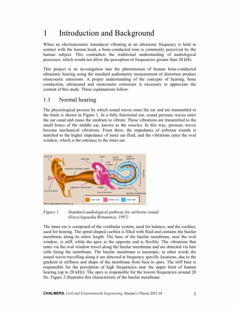
The physiological process by which sound waves enter the ear and are transmitted to
the brain is shown in Figure 1. In a fully functional ear, sound pressure waves enter
the ear canal and cause the eardrum to vibrate. These vibrations are transmitted to the
small bones of the middle ear, known as the ossicles. In this way, pressure waves
become mechanical vibrations. From there, the impedance of airborne sounds is
matched to the higher impedance of inner ear fluid, and the vibrations enter the oval
window, which is the entrance to the inner ear.
Figure 1 Standard audiological pathway for airborne sound
(Encyclopaedia Britannica, 1997)
The inner ear is composed of the vestibular system, used for balance, and the cochlea,
used for hearing. The spiral-shaped cochlea is filled with fluid and contains the basilar
membrane along its entire length. The base of the basilar membrane, near the oval
window, is stiff, while the apex at the opposite end is flexible. The vibrations that
enter via the oval window travel along the basilar membrane and are detected via hair
cells lining the membrane. The basilar membrane is tonotopic, in other words the
sound waves travelling along it are detected at frequency specific locations, due to the
gradient in stiffness and shape of the membrane from base to apex. The stiff base is
responsible for the perception of high frequencies near the upper limit of human
hearing (up to 20 kHz). The apex is responsible for the lowest frequencies around 20
Hz. Figure 2 illustrates this characteristic of the basilar membrane.

CHALMERS, Civil and Environmental Engineering, Master’s Thesis 2011:18 2
Figure 2 Tonotopic layout of the basilar membrane
(Encyclopaedia Britannica, 1997)
There are three rows of outer hair cells and one row of inner hair cells along the
length of the basilar membrane (see Figure 3). The outer hair cells are found along the
more moveable centre of the membrane, while the inner hair cells are located near the
anchored inner edge of the membrane. The outer hair cells can thus move and respond
to stimulus much more readily. They move actively, as well as passively, in response
to vibrations, as defined by their characteristic property of electromotility. The
tectorial membrane, which covers the rows of inner and outer hair cells, is firmly
linked to the stereocilia (hair bundles) at the tips of the outer hair cells. The inner hair
cells do not make contact with the tectorial membrane.
Figure 3 Cross-section of the cochlea (Fettiplace and Hackney, 2006)
The inner hair cells, the outer hair cells and the brain form an electromechanical
feedback loop. The inner hair cells send signals to the brain via afferent fibres of the
auditory nerve, while the outer hair cells receive signals from the brain via efferent
nerve fibres. When a sound wave travels along the basilar membrane, the inner hair
cells just barely respond, due to their location on the unmoveable part of the basilar
membrane. When the brain receives the very small signal being generated by the
scarcely moving inner hair cells, it sends a request via efferent nerve fibres to the
outer hair cells, requesting amplification. The outer hair cells respond to the incoming
sound waves by vibrating and changing shape. This increased motion causes the
attached tectorial membrane to move, pulling it toward and making contact with the
inner hair cells. This stimulates movement of the inner hair cells, and the information

CHALMERS, Civil and Environmental Engineering, Master’s Thesis 2011:18 3
is sent to the brain. If the signal is still not intense enough for the brain to perceive, it
will send another request. In this way, the movements of the basilar membrane are
accentuated in amplitude and frequency resolution and transmitted to the inner hair
cells and on to the brain. For this reason the outer hair cells are often known as
“cochlear amplifiers”.
1.2 Bone-conducted hearing
When a vibrating object makes contact with the human head, the vibrations can travel
through the bones of the skull directly to the inner ear, allowing a perception of sound
as the basilar membrane vibrates synchronously. A typical example of bone
conduction would be an oscillating tuning fork held to the forehead. The air-
conducted sound of the vibrating object may often be heard simultaneously as it
travels through the air into the outer and middle ear in the traditional way.
The bone-conducted signal bypasses the middle ear and any shortcomings it may
have. For example, a bone-anchored hearing aid uses bone conduction to enable
sufferers of conductive middle-ear hearing loss to perceive sound.
1.3 Ultrasonic hearing
The healthy, young human ear can normally detect sound waves that range from 20
Hz to 20 kHz, and never higher than 24 kHz (Lenhardt, 1991), although this upper
limit decreases gradually with age and exposure to noise. Sound waves with
frequencies above this range are known as ultrasonic, and cannot be heard by humans.
It has traditionally been assumed that the human audiological system is not designed
to respond to these high-frequency sounds. The impedance-matching function of the
middle ear, necessary to transmit sounds from the outer to the inner ear, is known to
be unable to handle ultrasonic frequencies (Pumphrey, 1950). Many animals can hear
much higher frequencies than 20 kHz; cats can hear over 60 kHz, dolphins can hear
up to 150 MHz.
Human bone-conducted ultrasonic hearing is a phenomenon in which vibrations even
greater than 20 kHz are perceived by humans when conducted through bones in the
skull. Normally this is achieved via a transducer applied to the mastoid or the
forehead. This phenomenon has been reported since the early 1950s (Deatherage,
1954). When subjects are asked to match this perceived tone to an audible pitch, they
generally choose a frequency between 13 and 16 kHz, or the highest frequency they
can hear. Those subjects who have high frequency hearing loss will often still detect a
sound, although the intensity may need to be increased to allow perception (Lenhardt,
1991).
Many theories have been put forward over the years and tested in an attempt to
explain what allows these signals to be heard. The following published studies present
different theories behind human bone-conducted ultrasonic hearing.
CHALMERS, Civil and Environmental Engineering, Master’s Thesis 2011:18 4
1.4 Theories about ultrasonic hearing
1.4.1 Non-cochlear receptor
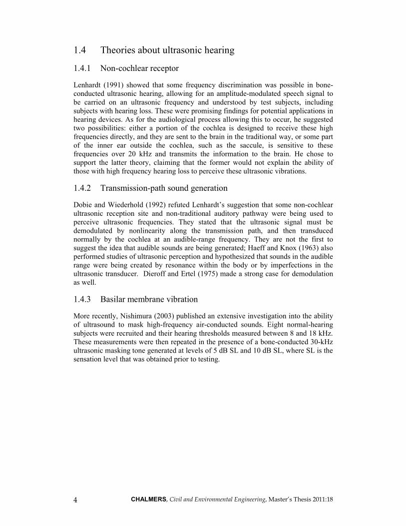
Lenhardt (1991) showed that some frequency discrimination was possible in bone-
conducted ultrasonic hearing, allowing for an amplitude-modulated speech signal to
be carried on an ultrasonic frequency and understood by test subjects, including
subjects with hearing loss. These were promising findings for potential applications in
hearing devices. As for the audiological process allowing this to occur, he suggested
two possibilities: either a portion of the cochlea is designed to receive these high
frequencies directly, and they are sent to the brain in the traditional way, or some part
of the inner ear outside the cochlea, such as the saccule, is sensitive to these
frequencies over 20 kHz and transmits the information to the brain. He chose to
support the latter theory, claiming that the former would not explain the ability of
those with high frequency hearing loss to perceive these ultrasonic vibrations.
1.4.2 Transmission-path sound generation
Dobie and Wiederhold (1992) refuted Lenhardt’s suggestion that some non-cochlear
ultrasonic reception site and non-traditional auditory pathway were being used to
perceive ultrasonic frequencies. They stated that the ultrasonic signal must be
demodulated by nonlinearity along the transmission path, and then transduced
normally by the cochlea at an audible-range frequency. They are not the first to
suggest the idea that audible sounds are being generated; Haeff and Knox (1963) also
performed studies of ultrasonic perception and hypothesized that sounds in the audible
range were being created by resonance within the body or by imperfections in the
ultrasonic transducer. Dieroff and Ertel (1975) made a strong case for demodulation
as well.
1.4.3 Basilar membrane vibration
More recently, Nishimura (2003) published an extensive investigation into the ability
of ultrasound to mask high-frequency air-conducted sounds. Eight normal-hearing
subjects were recruited and their hearing thresholds measured between 8 and 18 kHz.
These measurements were then repeated in the presence of a bone-conducted 30-kHz
ultrasonic masking tone generated at levels of 5 dB SL and 10 dB SL, where SL is the
sensation level that was obtained prior to testing.
CHALMERS, Civil and Environmental Engineering, Master’s Thesis 2011:18 5
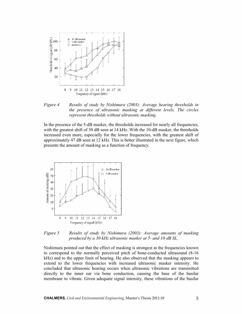
Figure 4 Results of study by Nishimura (2003): Average hearing thresholds in
the presence of ultrasonic masking at different levels. The circles
represent thresholds without ultrasonic masking.
In the presence of the 5-dB masker, the thresholds increased for nearly all frequencies,
with the greatest shift of 30 dB seen at 14 kHz. With the 10-dB masker, the thresholds
increased even more, especially for the lower frequencies, with the greatest shift of
approximately 47 dB seen at 12 kHz. This is better illustrated in the next figure, which
presents the amount of masking as a function of frequency.
Figure 5 Results of study by Nishimura (2003): Average amounts of masking
produced by a 30-kHz ultrasonic masker at 5- and 10-dB SL.
Nishimura pointed out that the effect of masking is strongest at the frequencies known
to correspond to the normally perceived pitch of bone-conducted ultrasound (8-16
kHz) and to the upper limit of hearing. He also observed that the masking appears to
extend to the lower frequencies with increased ultrasonic masker intensity. He
concluded that ultrasonic hearing occurs when ultrasonic vibrations are transmitted
directly to the inner ear via bone conduction, causing the base of the basilar
membrane to vibrate. Given adequate signal intensity, these vibrations of the basilar

CHALMERS, Civil and Environmental Engineering, Master’s Thesis 2011:18 6
membrane will spread downward toward the apex, allowing hair cells to respond that
are designed to normally pick up audible-range vibrations.
1.5 Otoacoustic emissions
Otoacoustic emissions (OAEs), discovered in 1978 by Dr. David Kemp, are low-level
sounds in the ear canal produced by the vibration of the outer hair cells in response to
sounds entering the cochlea. As explained in 1.1, the outer hair cells move actively in
response to stimuli; this electromechanical feedback serves to selectively amplify and
tune the vibrations on the basilar membrane. While this process contributes to the
signal being picked up by the inner hair cells and perceived by the brain, the same
vibrations are also transmitted back out the ear canal as sound waves, via the eardrum.
These sounds are usually too low to be audible, but can be measured with custom
instrumentation.
According to Kemp, the presence of otoacoustic emissions in an individual is an
indication of healthy hearing. The frequency at which an OAE can be measured is
more important than the specific intensity of that OAE, since measurement setup can
have an impact. A change in OAEs in a particular individual is an indication of a
change in cochlear function, but differences in OAE intensity between subjects cannot
be compared. An ear with damaged outer hair cells (but working inner hair cells) will
normally lose measurable OAEs, whereas an ear with damaged inner hair cells (but
working outer hair cells) may still have measurable OAEs. Loss of OAEs does not
necessarily indicate a loss of hearing, but rather a loss of amplitude and frequency
selectivity. Likely there are other parts of the ear that are involved as well, but the
outer hair cells take on the principal role in generating OAEs.
1.5.1 Measurement
Otoacoustic emissions can be measured using a probe microphone inserted into the
ear canal. The test is non-invasive and objective, not requiring any interaction from
the test subject. Otoacoustic emissions measurements are standard audiological tools
used in clinical hearing tests, especially on infants. The subject must have a working,
healthy middle ear, as the detection of OAEs can be affected by conductive losses.
Typically these measurements are taken in response to a particular stimulus: Transient
Evoked Otoacoustic Emissions (TEOAEs) normally make use of a click stimulus;
Distortion Product Otoacoustic Emissions (DPOAEs) involve two separate continuous
tones as stimuli.
The two stimuli used in DPOAEs are pure sinusoidal tones at two different
frequencies, f1 and f2, and two different sound pressure levels, L1 and L2. The
combination of these two tones in the ear generates otoacoustic emissions at other
frequencies, known as distortion product tones. These combinations, which can often
be heard by the test subject, are the result of non-linear intermodulation of the two
tones, and the resulting distortion products are known to satisfy the formula fdp = f1 +
N(f2-f1) (Kemp, 2002). The ratio between f1 and f2 and the individual levels of L1 and
L2 must be selected prior to testing to obtain maximum DPOAE levels. Several
combinations of sound levels and frequency ratios can be effective; in general L2 is
almost always chosen to be higher than L1 and f2/f1 is usually 1.2. The most
prominent DPOAE is usually found at fdp = 2f1-f2. Due to this known relationship

CHALMERS, Civil and Environmental Engineering, Master’s Thesis 2011:18 7
between the input and output frequencies of DPOAEs, these emissions are more
helpful than TEOAEs for studying the tonotopic function of the cochlea.
1.5.2 Suppression
The suppression of otoacoustic emissions is analogous to psychoacoustic masking of
audible stimuli (Kemp, 2002). In other words, a tone that masks a stimulus tone will
also suppress the otoacoustic emissions normally generated in the presence of that
stimulus. This means that emissions will be suppressed for frequencies at or close to
the masking tone frequency. In keeping with the analogy to psychoacoustic masking,
suppression contours have a similar shape to psychoacoustic tuning curves.
1.5.3 Plotting
When measuring DPOAE values of a subject, it is normally desirable to obtain the
results for a range of f1 and f2 values. For example, a test might measure the sound
level of the emission at fdp = 2f1-f2 generated when f2 = 2, 4, 6, 8 and 10 kHz, with a
constant relationship between f2 and f1. The results are then plotted on a graph known
as a DP-gram, shown in Figure 6. For each value of f2 along the x-axis, the sound
pressure level of the DPOAE at 2f1-f2 is plotted. In addition, the sound pressure level
of the two stimulus tones is plotted.
Figure 6 Example of a DP-gram.

CHALMERS, Civil and Environmental Engineering, Master’s Thesis 2011:18 8
2 Purpose
The purpose of this project was to use DPOAE measurements to better understand
bone-conducted ultrasound, and to localize where in the ear the ultrasonic signal may
be received and processed. DPOAE measurements should provide a view into the
operations of the inner ear in the presence of bone-conducted ultrasonic vibrations.
Any change in OAEs in the presence of an ultrasonic masker would indicate that the
cochlea is involved in hearing it. OAEs are very stable with time as the outer hair cells
do not get tired, and the repeatability is very high. DPOAEs were chosen here
because, unlike TEOAEs (see 1.5.1), they are known to have frequency characteristics
above 10 kHz, which is essential in this particular study since the frequency range
above 10 kHz is closer to the ultrasonic range, and most likely to be affected. Another
important property of DPOAEs is that when they are suppressed, the effect is similar
to psychoacoustic masking, because the emission will be suppressed when the ear is
stimulated at a neighbouring frequency.
Although it might seem natural to try to elicit DPOAEs using bone-conducted
ultrasonic stimuli, the goal in this study was to suppress DPOAEs elicited by airborne
audible-range sounds, using a bone-conducted ultrasonic masker. There are many
reasons for this indirect approach. It would be challenging to generate the required
levels for the two stimuli in the ultrasonic range. OAEs are produced by the outer hair
cells, and ultrasonic hearing has been shown not to involve outer hair cells (Ohyama
et al., 1985), but the cochlea may still be involved. Therefore, ultrasonic bone-
conducted stimuli are not expected to elicit OAEs directly (this was confirmed by an
informal test in the early days of the project). It is more likely that the effect of
ultrasonic frequencies on the cochlea could be shown by measuring how DPOAEs
created by air-conducted audible-range stimuli could be reduced by an ultrasonic
masking tone.
By using OAEs in this manner we can better understand the cochlea’s possible
function in hearing bone-conducted ultrasound, allowing us to compare and clarify the
current theories about bone-conducted ultrasonic hearing. If a bone-conducted
ultrasonic signal, presented as a masking signal, has any impact on the perception of
acoustic stimuli, or on OAEs produced, then this would help to localize where in the
auditory path the ultrasonic signal is being received and processed.
CHALMERS, Civil and Environmental Engineering, Master’s Thesis 2011:18 9
3 Hypothesis
The expected outcome of this study was based on the theory presented by Nishimura
about the downward spread of masking along the basilar membrane (see Section
1.4.4). The resulting assumption was that the cochlea is involved in ultrasonic
hearing. Specifically, in the presence of an ultrasonic masker, the basilar membrane
vibrates. Given strong enough vibrations, this allows the most basal inner hair cells,
which normally respond to audible-range high frequencies, to be excited. Therefore,
the expected result of this study was that the ultrasonic masking signal would have a
detrimental effect on the ability to perceive the two-tone audible-range stimulus at
high frequencies near the test subject’s upper limit of hearing, thereby reducing the
DPOAEs produced.

CHALMERS, Civil and Environmental Engineering, Master’s Thesis 2011:18 10
4 Measurement setup
In order to perform this test, each test subject had to have a small probe inserted into
one of their ears, containing a microphone and two speakers, and an ultrasonic
transducer mounted on a headband and pressed against their forehead. DPOAE testing
requires that a two-tone stimulus be played into the ear canal, and the response in the
ear be measured with the probe microphone. For this study, the test needed to be
performed in the absence and presence of the bone-conducted ultrasonic stimulus at
controlled, increasing sound levels. The following sections discuss the existing
standard measurement equipment and available software, and explain why a new
custom setup was required.
4.1 Standard otoacoustic measurement equipment
Commercial OAE units, such as the one made by BioLogic, do not allow for
experimentation in the 8-16 kHz range (the range of interest for this study). For this
reason, custom instrumentation was needed for this test. The custom equipment
already in use by Dr. Laura Dreisbach at San Diego State University was utilized. The
focus of Dr. Dreisbach’s work is the measurement of DPOAEs at frequencies greater
than 10 kHz, up to 16 kHz. Therefore her equipment was ideally suited to this
project’s testing, and has been proven to be reliable. Modifications were made to the
setup to incorporate the ultrasonic transducer designed by Dr. Gary Sokolich.
4.2 Custom DPOAE lab equipment
The following equipment is used by Dr. Dreisbach to make DPOAE measurements.
The external sound card is a MOTU 828 mkII audio processor with multiple inputs
and outputs. The ear probe is custom-made using a pair of modified Sennheiser CX-
300 earbuds. These are encased in two sealed metal cylinders, coupled to two 16-
gauge medical tubes. These tubes are then connected to an Etymotic Research ER-
10B+ emission probe microphone. The probe is capped with a foam probe tip and
inserted into the ear, as shown in Figure 7, thus allowing two separate audio input
channels and one output channel to be securely positioned in the ear canal.
Figure 7 The DPOAE ear probe, attached via tubes to the Sennheiser earbuds

CHALMERS, Civil and Environmental Engineering, Master’s Thesis 2011:18 11
4.3 Custom Ultrasonic test equipment
In addition to the DPOAE equipment normally used in this laboratory, additional
equipment was needed to create the ultrasonic tone. The ultrasonic transducer,
provided by Dr. Gary Sokolich, was composed of a piezoelectric transducer capable
of vibrating at frequencies between 25 and 45 kHz. The output of this transducer has
been tested to ensure that it is linear and contains no subharmonics. An HP467A
power amplifier plus a custom amplifier were used to power the transducer. Finally an
adjustable headband was designed for this study to allow consistent positioning of the
transducer on the subject’s forehead.
Figure 8 Ultrasonic transducer and headband
4.4 Standard test software
To run her tests and analyse the results, Dr. Dreisbach uses EMAV, a free program
created by Stephen Neely and Zhiqiang Liu of Boys Town National Research
Hospital for measuring and displaying otoacoustic emissions. This program does not
offer the flexibility of a third stimulus channel for the ultrasonic bone-conducted
signal to be presented simultaneously. In order to include the ultrasonic bone-
conducted signal in the automated test procedure, a new automated test procedure was
needed to present the sequence of tone pairs and ultrasonic stimuli to the listener,
record the resulting otoacoustic emissions, and plot the data.
4.5 Custom software
Although EMAV is a well-established, highly dependable program for measuring
DPOAEs up to 16 kHz or higher, it was not usable for this study. Firstly, it was
necessary to have control of three output signals (two for the stimulus tones and one
for the ultrasonic tone) while EMAV only controls two output signals. Also, the
sampling frequency in EMAV is 44 kHz, which would not accommodate a 30 kHz
output signal without any aliasing. In addition, more customisation was required for
the timing of the tones. Therefore, an automated test procedure was created in
MATLAB, with functionality based on EMAV.
The in-ear calibration portion of the EMAV test was still employed at the very
beginning of the test. Once the calibration was run, the resulting calibration output
data was entered into the new custom program; the remainder of the test was run by

CHALMERS, Civil and Environmental Engineering, Master’s Thesis 2011:18 12
the new program, based on this calibration data. The sampling frequency in the
custom software was 96 kHz, well over the Nyquist frequency of 60 kHz.
Generate tone
pair stimuli +
ultrasonic
masker
Start
Record response
in segments
Time average
segments
Noise floor
>
-15 dB SPL?
Subtract
alternating
segments
Repeat current
tone pair
Input panel
Response
spectrum
Noise floor
spectrum
FFT
FFT
Final tone pair?Advance to next
tone pair
Finish
3rd incidence
of high noise for
this tone pair?
Yes No
No
Yes Yes
No
DP-gram
Figure 9 Outline of custom software structure
The flow chart in Figure 9 outlines the basic structure of the MATLAB code. The test
begins with an input panel window, in which the test operator must enter the
following information: the subject calibration data file name and the subject’s
dynamic range for the ultrasonic tone (the threshold and the maximum comfortable
level in dB). As well, the operator must choose whether to generate an ultrasonic

CHALMERS, Civil and Environmental Engineering, Master’s Thesis 2011:18 13
signal for this round of testing, and what the level should be (0, 5, 10, 15, or 20 dB
SL). Following this, the test operator clicks a button to start the test.
The first tone pair is generated, starting randomly with either f2 = 2 kHz or f2 = 16
kHz. For each pair of frequencies, the stimulus tones are repeated 16 times to allow
for better averaging and a lower noise floor. The tone duration is 683 msec per
repetition, with a 200-msec pause between tones. The ultrasonic tone, if selected, is
generated simultaneously but held constant for 1.083 seconds, through the 16 tone-
pair repetitions, as this was deemed to be more comfortable to the subject. (These tone
durations were converted from number of samples to seconds, hence the awkward
numbers.) The frequency of the ultrasonic tone is 30 kHz. There is a 15-second gap
between primary pairs in order to give the test subject a short break.
The microphone probe records the response in the ear canal during the presentation of
each tone pair, capturing both the computer-generated tones and any otoacoustic
emissions. The recorded response is then split into 16 consecutive segments for
analysis. This follows the analysis procedure suggested by Dreisbach (2001). These
16 recorded segments are averaged in time to obtain a clean response, which is then
brought to the frequency domain via a Fast Fourier Transform. The result is a
spectrum of the response recorded in the ear canal. It is important to compare this
response to the noise floor in order to see how significant the results are. The noise
floor spectrum is obtained by subtracting the sum of the odd-numbered segments of
the recorded response from the sum of the even-numbered segments, dividing by 16,
and then taking the Fast Fourier Transform. In this way most constant noise, such as
line noise, will be reduced or eliminated. The spectra from the 16 tone pair repetitions
are then averaged, and the resulting response and noise floor spectra are displayed on
the computer screen. See Section 6.2, Figure 12 for an example.
The program then seeks the value of the response at 2f1 – f2 to determine if there is a
measurable DPOAE. The noise floor at 2f1 – f2 has to be less than –15 dB SPL for the
result to be valid. This value was chosen after many system trials to be the lowest
possible for this system. If the noise floor is acceptable, the value of the response is
recorded as the DPOAE for that tone pair, and displayed on the DP-gram on the
screen. If the noise floor is too high, the test starts over for that tone pair. To avoid
endless repetitions, the test will repeat only once for each tone pair, and then will skip
to the next tone pair, and no DPOAE is displayed on the DP-gram for that tone pair.
When the final tone pair is complete, the complete DP-gram is displayed and recorded
(as seen in Figure 6).

CHALMERS, Civil and Environmental Engineering, Master’s Thesis 2011:18 14
5 Test description
5.1 Test subjects
Test subjects had to have healthy ears, normal hearing and robust high-frequency
DPOAEs in order to be candidates for this study.
For each potential subject, both ears were examined and tested for middle ear
function. Following this, a Von Békésy hearing test was administered to determine
airborne hearing thresholds. Subjects needed to respond to tones at all tested
frequencies from 1 through 16 kHz, with thresholds ideally below 30 dB SPL for the
range of 1 to 8 kHz. If a subject’s thresholds were slightly outside this limit, they
could still qualify for the study if they had strong DPOAEs, as confirmed in the next
step of the screening.
Subjects were then screened for the presence of DPOAEs at 2f1-f2 for values of f2
from 16 kHz down to 1 kHz, in 1 kHz decrements. The frequency ratio (f2/f1) was
always 1.2 and the levels of the frequency primary tones were 57 and 45 dB SPL. The
stimulus levels were determined by an in-the-ear calibration procedure conducted at
the beginning of the test. In order to qualify for the test, the DPOAEs had to be at
least 5 dB above the noise floor at 2 through 8 kHz, and there had to be at least five
frequency points with measurable DPOAEs between 9 and 16 kHz.
Following this screening, 5 candidates were accepted for the study. Some candidates
had only one qualifying ear, resulting in 8 ears confirmed for the study. All candidates
were between the ages of 20 and 31; there were 5 female ears and 3 male ears.
The hearing thresholds for all accepted subjects are shown in Figure 10. Baseline
DPOAE levels for all subjects are shown in Figure 12 in Section 6.1.

CHALMERS, Civil and Environmental Engineering, Master’s Thesis 2011:18 15
1.0 4.0 8.0 10.0 12.5 14.0 16.0
f [kHz]
0
10
20
30
40
50
60
70
80
Hearing Threshold [dB SPL]
Figure 10 Combined hearing thresholds for all eight chosen candidate ears
The one subject with thresholds approaching 35 dB SPL for 2 and 8 kHz, seen as the
top line in Figure 10, was deemed an acceptable candidate after demonstrating very
strong DPOAEs in the 9 to 16 kHz range.
5.2 Test procedure
When one or both ears met the study criteria, the test commenced immediately. The
subject was given the ultrasonic transducer and asked to find the location on their
forehead at which the transducer would create a robust bone-conducted tone perceived
in the ear being studied. The headband was then attached securely to the subject’s
head to ensure that the transducer would remain in this location throughout the
testing. In order to determine the subject’s threshold and dynamic range, ultrasonic
tones were generated at incrementally decreasing and increasing levels, much like a
regular hearing test. The subject identified their maximum comfort level, with 20 dB
SL being the maximum level that was presented.
CHALMERS, Civil and Environmental Engineering, Master’s Thesis 2011:18 16
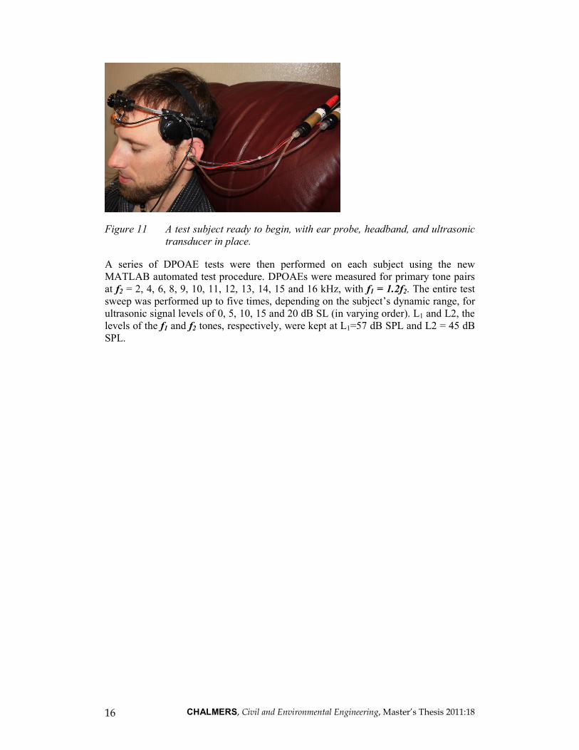
Figure 11 A test subject ready to begin, with ear probe, headband, and ultrasonic
transducer in place.
A series of DPOAE tests were then performed on each subject using the new
MATLAB automated test procedure. DPOAEs were measured for primary tone pairs
at f2 = 2, 4, 6, 8, 9, 10, 11, 12, 13, 14, 15 and 16 kHz, with f1 = 1.2f2. The entire test
sweep was performed up to five times, depending on the subject’s dynamic range, for
ultrasonic signal levels of 0, 5, 10, 15 and 20 dB SL (in varying order). L1 and L2, the
levels of the f1 and f2 tones, respectively, were kept at L1=57 dB SPL and L2 = 45 dB
SPL.

CHALMERS, Civil and Environmental Engineering, Master’s Thesis 2011:18 17
6 Results
Complete results were collected for the eight subject ears that met the stated
requirements.
6.1 Baseline emissions – all subjects
The baseline DPOAEs for all eight tested ears, without bone-conducted ultrasound,
are shown in a combined DP-gram below. (L1 = 57, L2 = 45, f1 = 1.2f2)
2 4 6 8 10 12 14 16
f2 [kHz]
-25
-20
-15
-10
-5
0
5
10
DPOAE at 2f 1-f2 [dB SPL]
Average noise floor
Figure 11 Subject baseline DPOAE levels for L1 = 57 dB, L2 = 45 dB, f1 = 1.2f2
Clearly there is great variation in otoacoustic emissions between all eight of these
healthy, normal ears. At the high frequencies, it is interesting to observe that many
ears have very low emissions at f2 = 12 kHz, and a peak in emissions at f2 = 13 kHz.
Above 13 kHz, most subject’s DPOAEs drop off quite quickly, although one subject
had significant emissions at f2 = 15 kHz. These results are highly repeatable for these
measurement conditions with L1 = 57 dB, L2 = 45 dB, and f1 = 1.2f2.

CHALMERS, Civil and Environmental Engineering, Master’s Thesis 2011:18 18
6.2 Sample individual output - without ultrasound
Figure 12 shows a screenshot from the testing software with a sample frequency
response as measured in a subject’s ear for a set of stimuli. The two stimuli, at f1 =
10.8 kHz and f2 = 13 kHz, are clearly seen on this spectrum. The DPOAE can also be
observed as a 2.8-dB spike at 2f1-f2 = 8.6 kHz. The average noise floor is seen at
approximately –20 dB.
Figure 12 Sample frequency spectrum of measurement taken with no bone-
conducted ultrasound
A screenshot of the resulting DP-gram for this same subject ear, as explained in
Section 1.5.3 and shown in Figure 6, is repeated in Figure 13. The DPOAE of 2.8 dB
from Figure 12 can be found in this DP-gram at f2 = 13 kHz.

CHALMERS, Civil and Environmental Engineering, Master’s Thesis 2011:18 19
Figure 13 Sample DP-gram plotting DPOAE levels for one subject taken with no
bone-conducted ultrasound
6.3 Sample individual output - with ultrasound
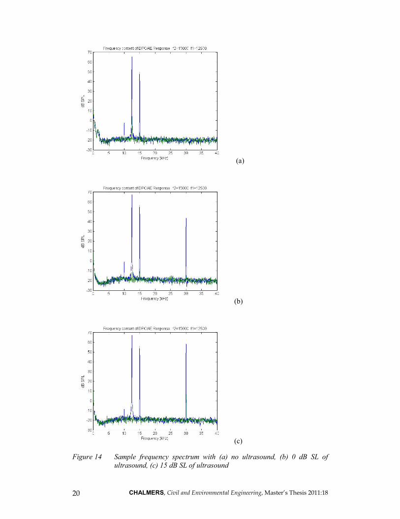
In the set of three figures that follow, displayed output is shown for one subject ear at
three different levels of bone-conducted ultrasound. The ear probe and the ultrasonic
transducer remained unmoved throughout the measurements. The stimulus tones were
identical for all three measurements: Tone 1 was 12.5 kHz and 62 dB SPL, and Tone
2 was 15 kHz and 50 dB SPL.
In Figure 14a, there is no ultrasonic masker signal. The stimulus tones and the
DPOAE at 10 kHz are seen clearly. In Figure 14b, the ultrasonic signal level is 0 dB
SL, the subject’s threshold. The 30-kHz signal is seen in the spectrum as a 40-dB
spike, showing that it is present in the ear canal. However, the DPOAE is relatively
unchanged from the no-ultrasound test condition. This demonstrates that an ultrasonic
signal at the subject’s threshold, and thus barely detectable to the subject, does not
have a noticeable impact on the subject’s DPOAEs. In the final figure, 14c, the
ultrasonic signal level is 15 dB SL, and it is seen in the spectrum as a spike at around
55 dB SPL, which is 15 dB higher than in the previous figure. In this case the DPOAE
is still there, but noticeably diminished by almost 10 dB. This agrees with the
hypothesis that the ultrasonic tone would suppress the DPOAE.
CHALMERS, Civil and Environmental Engineering, Master’s Thesis 2011:18 20
(a)
(b)
(c)
Figure 14 Sample frequency spectrum with (a) no ultrasound, (b) 0 dB SL of
ultrasound, (c) 15 dB SL of ultrasound

CHALMERS, Civil and Environmental Engineering, Master’s Thesis 2011:18 21
6.4 Averaged results for all subjects
The DPOAE levels at each tested frequency pair were plotted on a DP-gram. An
average DP-gram for all eight tested ears is shown in Figure 15.
Ultrasound Level None 0 dB SL 5 dB SL 10 dB SL 15 dB SL 20 dB SL
2 4 6 8 10 12 14 16
f2 [kHz]
-24
-22
-20
-18
-16
-14
-12
-10
-8
-6
-4
-2
0
2
DPOAE measured at 2f 1-f2 [dB SPL]
Average noise level
Figure 15 DPOAE levels averaged for all subjects
This figure contains 5 DPOAE curves for the five levels of ultrasonic signal: 0
through 20 dB above sensation level. Also plotted is the average noise floor. This
graph shows a clear difference between the DPOAEs measured at different levels of
ultrasound. In the presence of greater bone-conducted ultrasonic intensity, the strength
of the measured DPOAEs at the highest frequencies (8-16 kHz) is less. In addition,
this suppression of the DPOAEs increases with ultrasonic intensity, and its effects are
seen at increasingly lower stimulus frequencies.
Since most subject ears showed a peak in their baseline DPOAEs (section 7.1) at 13
kHz, this peak is also seen in these averaged results.
Table 1 summarizes the average shift in DPOAE levels at every frequency for every
bone-conducted ultrasound condition. Significant shifts (p < 0.05) are displayed in
bold.

CHALMERS, Civil and Environmental Engineering, Master’s Thesis 2011:18 22
Table 1 Average DPOAE level shift in the presence of each ultrasonic masker
Level shift [dB SL] per masker level: f2 [kHz]
0 dB SL 5 dB SL 10 dB SL 15 dB SL 20 dB SL
2 0.42 1.11 0.56 0.61 0.32
4 0.54 0.00 0.10 0.17 0.10
6 -0.24 -0.45 0.82 -0.58 -0.13
8 0.03 -1.01 -0.13 -1.25 -3.03
9 -0.41 -1.14 -1.32 -1.38 -4.17
10 -0.06 0.42 0.02 -2.32 -5.79
11 -1.81 -3.28 -2.95 -4.85 -9.25
12 0.11 0.41 -2.98 -6.00 -7.88
13 -1.03 -2.97 -4.84 -11.01 -12.46
14 0.45 -0.73 -1.88 -6.19 -6.74
15 -0.90 -1.64 -4.06 -4.94 -5.48
16 -0.54 -1.56 -3.55 -4.96 -4.44
Significant decreases in emissions are seen at 9-16 kHz with the 20 dB SL ultrasonic
tone, at 11-13 kHz and 16 kHz with 10 and 15 dB SL, and at 13 kHz with 5 dB SL.
There is no significant difference between the DPOAEs measured without ultrasound
and with ultrasound at the subject’s threshold (0 dB SL).
6.4.1 Averaged Results: Emission Suppression
Another way to look at the results is to plot the amount of DPOAE suppression
observed at different levels of bone-conducted ultrasound (the inverse of the above
table). DPOAE suppression is the difference in DPOAE level when measured with
and without the ultrasonic masking tone. This is shown in the following graph, with
the amount of suppression as a function of stimulus frequency for different intensities
of ultrasound.
CHALMERS, Civil and Environmental Engineering, Master’s Thesis 2011:18 23
Ultrasound Level None 0 dB SL 5 dB SL 10 dB SL 15 dB SL 20 dB SL
2 4 6 8 10 12 14 16
f2 [kHz]
-2
0
2
4
6
8
10
12
Average amount of DPOAE suppression at 2f 1-f2 [dB]
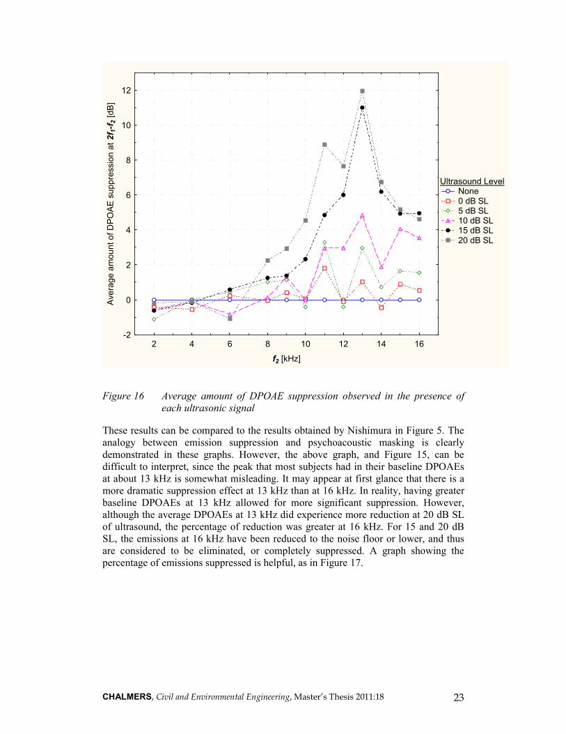
Figure 16 Average amount of DPOAE suppression observed in the presence of
each ultrasonic signal
These results can be compared to the results obtained by Nishimura in Figure 5. The
analogy between emission suppression and psychoacoustic masking is clearly
demonstrated in these graphs. However, the above graph, and Figure 15, can be
difficult to interpret, since the peak that most subjects had in their baseline DPOAEs
at about 13 kHz is somewhat misleading. It may appear at first glance that there is a
more dramatic suppression effect at 13 kHz than at 16 kHz. In reality, having greater
baseline DPOAEs at 13 kHz allowed for more significant suppression. However,
although the average DPOAEs at 13 kHz did experience more reduction at 20 dB SL
of ultrasound, the percentage of reduction was greater at 16 kHz. For 15 and 20 dB
SL, the emissions at 16 kHz have been reduced to the noise floor or lower, and thus
are considered to be eliminated, or completely suppressed. A graph showing the
percentage of emissions suppressed is helpful, as in Figure 17.
CHALMERS, Civil and Environmental Engineering, Master’s Thesis 2011:18 24
Ultrasound Level None 0 dB SL 5 dB SL 10 dB SL 15 dB SL 20 dB SL
2 4 6 8 10 12 14 16
f2 [kHz]
0
20
40
60
80
100
120
Percentage of baseline DPOAE [%]
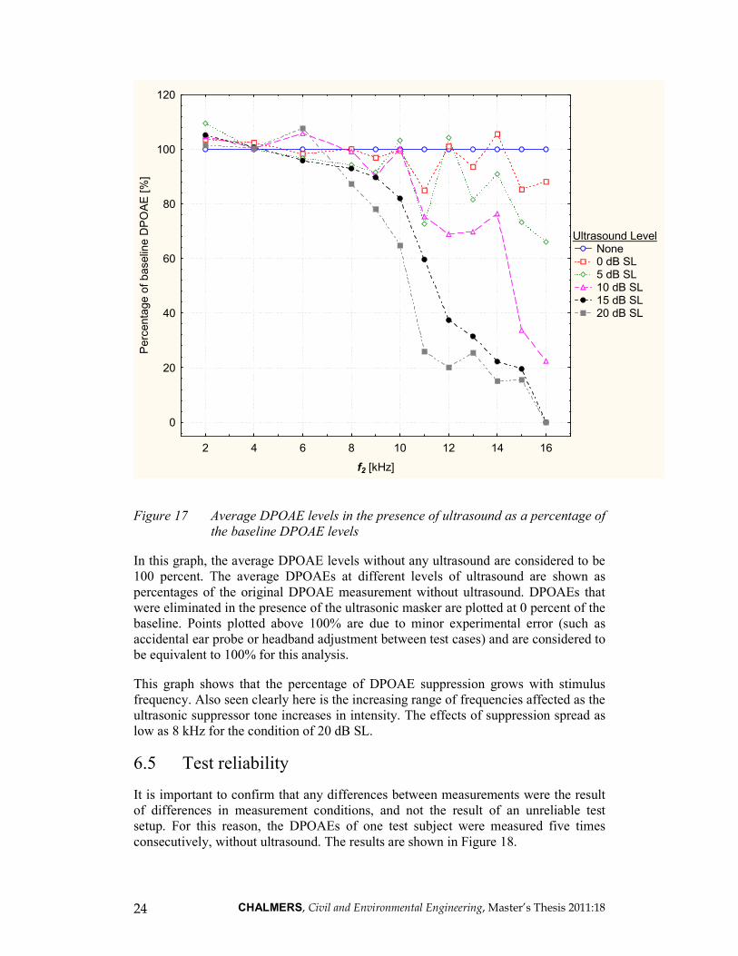
Figure 17 Average DPOAE levels in the presence of ultrasound as a percentage of
the baseline DPOAE levels
In this graph, the average DPOAE levels without any ultrasound are considered to be
100 percent. The average DPOAEs at different levels of ultrasound are shown as
percentages of the original DPOAE measurement without ultrasound. DPOAEs that
were eliminated in the presence of the ultrasonic masker are plotted at 0 percent of the
baseline. Points plotted above 100% are due to minor experimental error (such as
accidental ear probe or headband adjustment between test cases) and are considered to
be equivalent to 100% for this analysis.
This graph shows that the percentage of DPOAE suppression grows with stimulus
frequency. Also seen clearly here is the increasing range of frequencies affected as the
ultrasonic suppressor tone increases in intensity. The effects of suppression spread as
low as 8 kHz for the condition of 20 dB SL.
6.5 Test reliability
It is important to confirm that any differences between measurements were the result
of differences in measurement conditions, and not the result of an unreliable test
setup. For this reason, the DPOAEs of one test subject were measured five times
consecutively, without ultrasound. The results are shown in Figure 18.

CHALMERS, Civil and Environmental Engineering, Master’s Thesis 2011:18 25
0 2 4 6 8 10 12 14 16 18
f2 [kHz]
-22
-20
-18
-16
-14
-12
-10
-8
-6
-4
-2
0
2
4
DPOAE at 2f 1-f2 [dB SPL]
Figure 18 A standard DPOAE test performed five times sequentially to show
equipment reliability
Visually, these five curves appear almost identical. Numerically, the reliability can be
expressed in terms of three-sigma (3σ). The three-sigma rule states that for a normal
distribution of results, nearly all values lie within 3 standard deviations of the mean.
The three-sigma value per frequency of measurement is shown in Figure 19, along
with some of the suppression curves from Figure 16 as a comparison.
Ultrasonic Level
10 dB SL
15 dB SL
20 dB SL
3-sigma
2 4 6 8 10 12 14 16
f2 [kHz]
-2
0
2
4
6
8
10
12
14
dB
Figure 19 3-sigma plot juxtaposed with average amount of DPOAE suppression
In this case, the average 3σ is 1.57 dB. This indicates that nearly all values at each
frequency point, on average, lie within 1.57 dB of the average. A larger drop from the
mean would thus indicate a change in measurement conditions, not just test variation.
This is a very small range, considering that the amount of suppression that has been
CHALMERS, Civil and Environmental Engineering, Master’s Thesis 2011:18 26
observed in this experiment is as much as 10 dB. In fact, this average 3-sigma would
be even lower if the 16-kHz point were left out of the results. The 3-sigma at 16 kHz
is 4.48 dB. The measurements at 16 kHz are thus the least reliable. The average 3-
sigma for 2-15 kHz is 1.3 dB.

CHALMERS, Civil and Environmental Engineering, Master’s Thesis 2011:18 27
7 Discussion
These test results unquestionably show the suppression of DPOAEs created by air-
conducted audible-range stimuli by the bone-conducted ultrasonic masking tone. This
indicates that the cochlea was significantly involved in hearing the tone. Other parts
of the ear, brain or elsewhere may also be involved, but the cochlea is a critical
component in the process. If the cochlea played only a small role, or were not
involved at all, and some other part of the inner ear outside the cochlea was
responsible instead (as suggested by Lenhardt, 1991), these DPOAEs would not be
affected by the presence of the masker.
No subharmonics of the ultrasonic signal were measured in the ear canal. See Figure
14, which shows that the two stimulus tones, the DPOAE at 2f1-f2 and the pure
ultrasonic tone at 30 kHz were the only tones recorded in the ear canal. This indicates
that there was no measurable demodulation of the ultrasonic tone. If the ultrasonic
signal were demodulated by nonlinearity along the transmission path through the head
(as suggested by Dobie, R.A., Wiederhold, M.L.), then there would be noticeable
subharmonics of the 30-kHz tone in the frequency content measured at the ear.
Even if there were subharmonics of the ultrasonic signal present somewhere in the
head that were too low to be recorded in the ear canal, they could not account for the
dramatic impact on the DPOAEs seen here. The suppression of DPOAEs observed is
much more substantial than it would be with even an audible-range suppressor at such
a low level. For example, Gorga and Neely et al. (2003) observed that for a stimulus
pair where L2 is 50 dB SPL, a suppressor tone of similar frequency to f2 was only
effective at suppressing the DPOAEs if it were above 40 dB SPL. In contrast, the
bone-conducted ultrasonic tone in this study was 20 dB above sensation level at its
highest, with stimulus tones of L1 = 57 dB and L2 = 45 dB.
The DPOAEs were reduced the most at the higher frequencies of 13-16 kHz, near the
test subjects’ upper limit of hearing. With increasing intensity, the bone-conducted
ultrasonic signal masked a wider band of DPOAEs, starting with the highest
frequencies and spreading downward. It is thus possible that ultrasonic vibrations do
elicit vibrations of the basilar membrane, and that in the presence of an intense bone-
conducted ultrasonic masker, the basilar membrane responds with strong enough
vibrations that the most basal inner hair cells are excited. These inner hair cells are not
designed to normally pick up frequencies above 20 kHz. However, inner hair cells can
respond to sounds on their own (without the aid of the amplifying outer hair cells) if
intensity is sufficiently high. The inner hair cells do not have much frequency
selectivity, but as long as they are vibrating there will be a perception of sound, even
if it isn’t heard at the correct pitch. With increased ultrasonic intensity, a larger
section of the basal end of the basilar membrane is excited.
This supports the theory of Nishimura, T. et al that a downward spread of vibration
along the basilar membrane allows hair cells to respond that are designed to normally
pick up audible-range vibrations. Ultrasonic bone-conducted stimuli do not elicit
OAEs directly, meaning that ultrasonic hearing must activate inner hair cells only.
These suppressed DPOAEs would then correspond to the frequencies at which the
masker is perceived.
CHALMERS, Civil and Environmental Engineering, Master’s Thesis 2011:18 28
8 Conclusions
Distortion product otoacoustic emissions created by air-conducted audible-range
stimuli at frequencies near the upper limit of hearing can be suppressed in humans
with a bone-conducted ultrasonic signal. This confirms the involvement of the cochlea
in bone-conducted ultrasonic hearing.
In addition, increasing the intensity of bone-conducted ultrasound results in increased
suppression of DPOAEs over a wider range of high frequencies, indicating a
downward spread of vibration along the basilar membrane. This supports the theory
that perception of bone-conducted ultrasonic signals is caused by the excitation of the
most basal inner hair cells due to intense vibrations of the basilar membrane.

CHALMERS, Civil and Environmental Engineering, Master’s Thesis 2011:18 29
9 Future work
This study is the first step toward a new direction of investigation into the workings of
bone-conducted ultrasound. Now that it has been established that DPOAEs can be
suppressed by a bone-conducted ultrasonic tone, it seems likely that further testing
would be successful. As a start, testing a greater number of subjects could strengthen
the results of this study. Also, subjects with different degrees of high frequency
hearing loss could be tested, provided that they still had DPOAEs at some
frequencies. It would be interesting to observe what intensity of ultrasound would be
required in order for them to perceive the tone, as well as to suppress their DPOAES.
Additionally, these tests were conducted with a 30-kHz ultrasonic tone; other
ultrasonic frequencies could be experimented with. However, previous studies have
not found that the frequency of the ultrasound had a significant impact on perception
(such as in Nishimura’s 2003 study).
The scope of this study could also be expanded upon with other forms of testing.
Psychoacoustical masking tests, similar to what was done by Nishimura, could be
performed on the same test subjects that were used for this study, and resulting
masking curves could be compared with their DPOAE suppression curves. Another
type of objective testing would be Auditory Brainstem Response (ABR), in which the
subject’s neuronal action potentials are monitored by electrodes placed on the scalp in
response to auditory stimuli, in order to determine if there is an impact on the signal
being sent to the brain via the auditory nerve. This trio of testing (psychoacoustical,
DPOAE and ABR) could provide a comprehensive picture of the impacts on these test
subjects.
The same subjects could also participate in pitch-matching exercises, in which they
are presented with a bone-conducted ultrasonic tone and a controllable air-conducted
tone. The subject would adjust the air-conducted tone until it matched their perception
of the bone-conducted ultrasonic tone.
Provided that this further testing continues to support the conclusions stated here, an
important application of bone-conducted ultrasound is as an alternative hearing aid
technology, through the use of amplitude modulation on an ultrasonic carrier
frequency. Candidates would have significant high frequency hearing loss and middle
ear disorders. As well, bone-conducted ultrasound is currently being used as a type of
treatment for people suffering from tinnitus. Furthering the knowledge about bone-
conducted ultrasound could provide some insight into the role of the inner ear in
tinnitus and the ability to provide better treatment.
CHALMERS, Civil and Environmental Engineering, Master’s Thesis 2011:18 30
10 References
Deatherage, B.H., Jeffress, L.A., Blodgett, H.C. (1954): A note on the audibility of
intense ultrasonic sound. Journal of the Acoustical Society of America, Vol. 26, No. 4,
1954, p. 582.
Dieroff, H.G., Ertel, H. (1975): Some thoughts on the perception of ultrasonics by
man. European Archives of Oto-Rhino-Laryngology, Vol. 209, No. 4, 1975, pp. 277-
290.
Dobie, R.A., Wiederhold, M.L. (1992): Ultrasonic hearing. Science, Vol. 255, 1992,
p. 1584.
Dreisbach, L.E., Siegel, J.H. (2001): Distortion-product otoacoustic emissions
measured at high frequencies in humans. Journal of the Acoustical Society of
America, Vol. 110, No. 5, 2001, pp. 2456-2469.
Dreisbach, L.E., Long, K.M., Lees, S.E. (2006): Repeatability of high-frequency
distortion-product otoacoustic emissions in normal-hearing adults. Ear & Hearing,
Vol. 27, No. 5, 2006, pp. 466-479.
Encyclopaedia Britannica, Inc. (1997): Human Ear. Encyclopaedia Britannica, 2011,
http://www.britannica.com/EBchecked/topic/175622/human-ear.
Fettiplace, R., Hackney, C.M. (2006): The sensory and motor roles of auditory hair
cells. Nature Reviews Neuroscience, Vol. 7, January 2006, pp. 19-29.
Gorga, M.P., Neely, S.T., et al. (2003): Distortion product otoacoustic emission
suppression tuning curves in normal-hearing and hearing-impaired human ears.
Journal of the Acoustical Society of America, Vol. 114, No. 1, 2003, pp. 263-278.
Haeff, A.V., Knox, C. (1962): Perception of ultrasound. Science, Vol. 139, 1963, pp.
590-592.
Kemp, D.T. (2002): Otoacoustic emissions, their origin in cochlear function, and use.
British Medical Bulletin 2002, Vol. 63, 2002, pp. 223-241.
Lenhardt, M.L., Skellett, R., et al. (1992): Human ultrasonic speech perception.
Science, Vol. 253, 1991, pp. 82-85.
Neely, S., Liu, Z. (2001): EMAV: Otoacoustic emission averager. Technical
Memorandum. Boys Town National Research Hospital, Omaha, USA, 26 pp.
Nishimura, T., Nakagawa, S., et al. (2003): Ultrasonic masker clarifies ultrasonic
perception in man. Hearing Research, Vol. 175, 2003, pp. 171-177.
Ohyama, K., Kusakari, J., Kawamoto, K. (1985): Ultrasonic electrocochleography in
guinea pig. Hearing Research, Vol. 17, 1985, pp. 143-151.
Pumphrey, R.J. (1950): Upper limit of frequency for human hearing. Nature, Vol.
166, 1950, p. 571.

CHALMERS, Civil and Environmental Engineering, Master’s Thesis 2011:18 31
Appendix A Matlab code for DPOAE tests
% Distortion Product OAE test for ultrasonic hearing study % Created by Jennifer Martin-Roff and Ben Sheffield clear all %%%%%%%%%% Begin Parameter Initialization Section %%%%%%%%%% %%%SYSTEM PARAMETERS%%% Fs = 96000; %sample rate is 96 kHz sweeps = 16; %# of sweeps (total recording buffers per set) sets = 16; %# of times primary pair is repeated (must be even); buf_size = 4096; %# of samples per sweep (recording buffer size) gap_btwn_sets = 0.200; %silence between sets (seconds) % bcu_cf = 30000; % Ultrasonic frequency Tonoffset = .200; % BCU offset from primary tones for on/off %%%STIMULUS PARAMETERS%%% f2 = [2; 4; 6; 8; 9; 10; 11; 12; 13; 14; 15; 16]; %f2 frequencies (kHz) f2_f1_ratio = 1.2; %ratio to calculate f1 from f2 L1_SPL = 57; %desired f1 level (dB SPL) L2_SPL = 45; %desired f2 level (dB SPL) %%% NOISE FLOOR DECISION PARAMETERS %%% nnsb = 10; %number of noise side bands (# of samples on either side of DP to calculate noise floor) nf_max = -15; %maximum allowable noise floor max_repeat = 2; %maximum number of times the tone pair will be repeated %%%DISPLAY PARAMETERS%%% fmin=20; %min abscissa (Hz) fmax=40000; %max abscissa (Hz) %%%CALIBRATION PARAMETERS SDSU%%% DA1_sens = 0.3226; %cnt_0toPk / Vrms DA2_sens = 0.3226; %cnt_0toPk / Vrms transducer_sens = 112; %SPL/Vrms; ER-2s = 100; CX-300s = 112; L = 84; %cnt adjustment for transducer 1 R = 124; %cnt adjustment for transducer 2 AD_sens = 0.0598; %cnt_rms / Vrms probe_sens = 1.75; %probe mic sensitivity (V/Pa) %%%%%%%%%% End Parameter Initialization Section %%%%%%%%%% %%%%%%%%%% Begin Stimulus Definition Section %%%%%%%%%% f2 = f2*1000; %convert to Hz num_tones = length(f2); %number of tone pairs presented % randomize order of frequency sweep (down by default) if rand < 0.5 f2 = flipud(f2) %sweep up end f1 = f2/f2_f1_ratio; %calculate f1 primary tones (Hz) risetime = 0.01; % ramp up 10 msec fcr = (acos(-1)-acos(1))/(2*pi*risetime); x = 1:round(risetime*Fs); crr = (0.5+cos(pi+2*pi*fcr*x/Fs)/2)'; %onset crf = (0.5+cos(2*pi*fcr*x/Fs)/2)'; %offset %%% Load EMAV Calibration file and adjust L1 and L2 values %%% cal_filename = get(findobj('tag','cal_file'),'string'); %Get EMAV Calibration File Name from GUI [cal_freq_scale,cal_L,cal_R,val_1k_L,val_1k_R] = cal2mat(cal_filename); cal_tones_L = spline(cal_freq_scale*1000,cal_L,f2); cal_tones_R = spline(cal_freq_scale*1000,cal_R,f1); Loffset = cal_tones_L - val_1k_L; Roffset = cal_tones_R - val_1k_R;

CHALMERS, Civil and Environmental Engineering, Master’s Thesis 2011:18 32
L2_SPL_correct = L2_SPL - Loffset; % Corrected L2 in dBSPL L1_SPL_correct = L1_SPL - Roffset; L2_V = 10.^((L2_SPL_correct-transducer_sens)/20); %convert from desired SPL to Volts for Sennheiser CX-300 L1_V = 10.^((L1_SPL_correct-transducer_sens)/20); %convert from desired SPL to Volts for Sennheiser CX-300 L2 = DA1_sens*L*L2_V; %level of test tone 1 (cnt) L1 = DA2_sens*R*L1_V; %level of test tone 2 (cnt) for m=1:num_tones if L2(num_tones+1-m,1) >= 1 L2(num_tones+1-m,1) = 0.999; disp(['L2 saturated at : ' num2str(f2(num_tones+1-m,1))]) end if L1(num_tones+1-m,1) >= 1 L1(num_tones+1-m,1) = 0.999; disp(['L1 saturated at : ' num2str(f1(num_tones+1-m,1))]) end end prim_dur = sweeps*buf_size; %primary tone duration (samples) prim_dur_sec = prim_dur/Fs; %primary tone duration (seconds) T = 0:1/Fs:prim_dur_sec-1/Fs; %period of each primary tone set bcu_dur_sec = prim_dur_sec+2*Tonoffset; %Ultrasonic tone duration (sec) bcu_dur = bcu_dur_sec*Fs; %Ultrasonic tone duration (samples) t_bcu = 0:1/Fs:bcu_dur_sec-1/Fs; %period of each ultrasonic tone set t_bcu_onoffset = zeros(round(Tonoffset*Fs),2); %%%%%%%%%% Open audio channels ao1 = analogoutput('winsound',5); % 5 = lab, 0 = home addchannel(ao1,1:2); set(ao1,'StandardSampleRates','Off'); ao1_props = propinfo(ao1, 'SampleRate'); set(ao1,'SampleRate',Fs); ao2 = analogoutput('winsound',4); % 5 = lab, 0 = home addchannel(ao2,1:2); set(ao2,'StandardSampleRates','Off'); ao2_props = propinfo(ao2, 'SampleRate'); set(ao2,'SampleRate',Fs); ai = analoginput('winsound',4); % 4 = lab, 0 = home addchannel(ai,1); set(ai,'StandardSampleRates','Off'); ai_props = propinfo(ai, 'SampleRate'); set(ai,'SampleRate',Fs) set([ai ao1 ao2],'TriggerType','Manual') set(ai,'ManualTriggerHwOn','Trigger') %%%Initialize Data%%% DPgram = []; %DPgram starts out blank DPgram_scale = []; %DPgram scale starts blank f1_levels = []; f2_levels = []; nf_levels = []; resp_per_pair=[]; nf_per_pair=[]; repeat_tp = 0; %%% START LOOP %%% %Create primary tones i=1; while i <= num_tones tonef2 = sin(2*pi*f2(num_tones+1-i)*T)'; tonef2(1:length(crr)) = tonef2(1:length(crr)).*crr; tonef2((end-length(crf)+1):end) = tonef2((end-length(crf)+1):end).*crf; tonef2 = L2(num_tones+1-i)*tonef2; tonef1 = sin(2*pi*f1(num_tones+1-i)*T)'; tonef1(1:length(crr)) = tonef1(1:length(crr)).*crr;

CHALMERS, Civil and Environmental Engineering, Master’s Thesis 2011:18 33
tonef1((end-length(crf)+1):end) = tonef1((end-length(crf)+1):end).*crf; tonef1 = L1(num_tones+1-i)*tonef1; bcu_cf = 1000*str2num(get(findobj('tag','cf_mask'),'string')); BCU_Level = str2num(get(findobj('tag','BCU_Level'),'string')); tonesupp = sin(2*pi*bcu_cf*t_bcu)'; tonesupp(1:length(crr)) = tonesupp(1:length(crr)).*crr; tonesupp((end-length(crf)+1):end) = tonesupp((end-length(crf)+1):end).*crf; tonesupp = 10^(BCU_Level/20).*tonesupp; empty = zeros(length(tonesupp),1); tonesupp = [tonesupp empty]; set_gap = zeros(gap_btwn_sets*Fs,2); y1 = [t_bcu_onoffset; tonef2 tonef1; t_bcu_onoffset; set_gap; ... t_bcu_onoffset; tonef2 tonef1; t_bcu_onoffset; set_gap; ... t_bcu_onoffset; tonef2 tonef1; t_bcu_onoffset; set_gap; ... t_bcu_onoffset; tonef2 tonef1; t_bcu_onoffset; set_gap; ... t_bcu_onoffset; tonef2 tonef1; t_bcu_onoffset; set_gap; ... t_bcu_onoffset; tonef2 tonef1; t_bcu_onoffset; set_gap; ... t_bcu_onoffset; tonef2 tonef1; t_bcu_onoffset; set_gap; ... t_bcu_onoffset; tonef2 tonef1; t_bcu_onoffset; set_gap; ... t_bcu_onoffset; tonef2 tonef1; t_bcu_onoffset; set_gap; ... t_bcu_onoffset; tonef2 tonef1; t_bcu_onoffset; set_gap; ... t_bcu_onoffset; tonef2 tonef1; t_bcu_onoffset; set_gap; ... t_bcu_onoffset; tonef2 tonef1; t_bcu_onoffset; set_gap; ... t_bcu_onoffset; tonef2 tonef1; t_bcu_onoffset; set_gap; ... t_bcu_onoffset; tonef2 tonef1; t_bcu_onoffset; set_gap; ... t_bcu_onoffset; tonef2 tonef1; t_bcu_onoffset; set_gap; ... t_bcu_onoffset; tonef2 tonef1; t_bcu_onoffset]; y2 = [tonesupp; set_gap; tonesupp; set_gap; ... tonesupp; set_gap; tonesupp; set_gap; ... tonesupp; set_gap; tonesupp; set_gap; ... tonesupp; set_gap; tonesupp; set_gap; ... tonesupp; set_gap; tonesupp; set_gap; ... tonesupp; set_gap; tonesupp; set_gap; ... tonesupp; set_gap; tonesupp; set_gap; ... tonesupp; set_gap; tonesupp]; set(ai, 'SamplesPerTrigger', length(y2)) putdata(ao1,y1) putdata(ao2,y2) start([ai ao1 ao2]) trigger([ai ao1 ao2]) % aitime = ai.InitialTriggerTime; % aotime = get(ao,'InitialTriggerTime'); % delay = aitime(6) - aotime(6); % delay = round(0.02*Fs); wait(ao2,length(y2)) recorded_data = getdata(ai); %%%%%%%%%%%%%%%%%%%%%%%%%%%%%%%%%%%%%%%%%%%%%%%%%%%%%%%%%%%%%%%%%%%%%%%%%%%%%%%%%%%%%%%%%%%%%%%% %%%%%%%%%% Begin Response Analysis Section %%%%%%%%%% % Section the recorded sets into sweep segments (time domain) resp_avg_t=[]; %initiate response average per sweep (time domain) noise_est_t=[]; %initiate noise floor estimate per sweep (time domain) recorded_data = recorded_data/AD_sens; %convert from cnt to V recorded_data = recorded_data/probe_sens; %convert from V to Pa gap = length(set_gap); onoffset = length(t_bcu_onoffset); resp_set1 = recorded_data(1*onoffset+0*(prim_dur+gap)+1 : 1*onoffset+1*prim_dur+0*gap,1); resp_set2 = recorded_data(3*onoffset+1*(prim_dur+gap)+1 : 3*onoffset+2*prim_dur+1*gap,1);
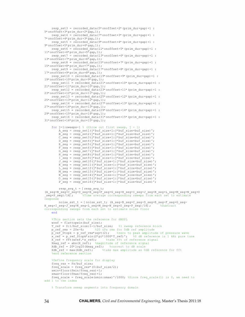
CHALMERS, Civil and Environmental Engineering, Master’s Thesis 2011:18 34
resp_set3 = recorded_data(5*onoffset+2*(prim_dur+gap)+1 : 5*onoffset+3*prim_dur+2*gap,1); resp_set4 = recorded_data(7*onoffset+3*(prim_dur+gap)+1 : 7*onoffset+4*prim_dur+3*gap,1); resp_set5 = recorded_data(9*onoffset+4*(prim_dur+gap)+1 : 9*onoffset+5*prim_dur+4*gap,1); resp_set6 = recorded_data(11*onoffset+5*(prim_dur+gap)+1 : 11*onoffset+6*prim_dur+5*gap,1); resp_set7 = recorded_data(13*onoffset+6*(prim_dur+gap)+1 : 13*onoffset+7*prim_dur+6*gap,1); resp_set8 = recorded_data(15*onoffset+7*(prim_dur+gap)+1 : 15*onoffset+8*prim_dur+7*gap,1); resp_set9 = recorded_data(17*onoffset+8*(prim_dur+gap)+1 : 17*onoffset+9*prim_dur+8*gap,1); resp_set10 = recorded_data(19*onoffset+9*(prim_dur+gap)+1 : 19*onoffset+10*prim_dur+9*gap,1); resp_set11 = recorded_data(21*onoffset+10*(prim_dur+gap)+1 : 21*onoffset+11*prim_dur+10*gap,1); resp_set12 = recorded_data(23*onoffset+11*(prim_dur+gap)+1 : 23*onoffset+12*prim_dur+11*gap,1); resp_set13 = recorded_data(25*onoffset+12*(prim_dur+gap)+1 : 25*onoffset+13*prim_dur+12*gap,1); resp_set14 = recorded_data(27*onoffset+13*(prim_dur+gap)+1 : 27*onoffset+14*prim_dur+13*gap,1); resp_set15 = recorded_data(29*onoffset+14*(prim_dur+gap)+1 : 29*onoffset+15*prim_dur+14*gap,1); resp_set16 = recorded_data(31*onoffset+15*(prim_dur+gap)+1 : 31*onoffset+16*prim_dur+15*gap,1); for j=1:sweeps-1 % (throw out first sweep, j = 1) A_seg = resp_set1(j*buf_size+1:j*buf_size+buf_size)'; B_seg = resp_set2(j*buf_size+1:j*buf_size+buf_size)'; C_seg = resp_set3(j*buf_size+1:j*buf_size+buf_size)'; D_seg = resp_set4(j*buf_size+1:j*buf_size+buf_size)'; E_seg = resp_set5(j*buf_size+1:j*buf_size+buf_size)'; F_seg = resp_set6(j*buf_size+1:j*buf_size+buf_size)'; G_seg = resp_set7(j*buf_size+1:j*buf_size+buf_size)'; H_seg = resp_set8(j*buf_size+1:j*buf_size+buf_size)'; I_seg = resp_set9(j*buf_size+1:j*buf_size+buf_size)'; J_seg = resp_set10(j*buf_size+1:j*buf_size+buf_size)'; K_seg = resp_set11(j*buf_size+1:j*buf_size+buf_size)'; L_seg = resp_set12(j*buf_size+1:j*buf_size+buf_size)'; M_seg = resp_set13(j*buf_size+1:j*buf_size+buf_size)'; N_seg = resp_set14(j*buf_size+1:j*buf_size+buf_size)'; O_seg = resp_set15(j*buf_size+1:j*buf_size+buf_size)'; P_seg = resp_set16(j*buf_size+1:j*buf_size+buf_size)'; resp_avg_t = [resp_avg_t; (A_seg+B_seg+C_seg+D_seg+E_seg+F_seg+G_seg+H_seg+I_seg+J_seg+K_seg+L_seg+M_seg+N_seg+O_seg+P_seg)/16]; %Time average corresponding sweeps from each set to estimate response noise_est_t = [noise_est_t; (A_seg-B_seg+C_seg-D_seg+E_seg-F_seg+G_seg-H_seg+I_seg-J_seg+K_seg-L_seg+M_seg-N_seg+O_seg-P_seg)/16]; %Subtract corresponding sweeps from each set to estimate noise floor end %This section sets the reference for dBSPL wref = flattopwin(buf_size); T_ref = 0:1/buf_size:1-1/buf_size; %1 sweep reference block p_ref_rms = 20e-6; %20 uPa rms for 0dB ref amplitude p_ref_0topk = p_ref_rms*sqrt(2); %zero to peak amplitude of pressure wave x_ref = p_ref_0topk*sin(2*pi*1000*T_ref)'; %0 dB reference is 1 kHz pure tone X_ref = fft(wref.*x_ref); %take fft of reference signal Xmag_ref = abs(X_ref); %magnitude of reference signal Xdb_ref = 20*log10(Xmag_ref); %convert to dB scale Xdb_ref = max(Xdb_ref); %take max amplitude as 0dB reference for fft %end reference section %Define frequency scale for display freq_res = Fs/buf_size; freq_scale = freq_res*(0:buf_size/2); smin=floor(fmin/freq_res)+1; smax=floor(fmax/freq_res)+1; freq_scale = freq_scale(smin:smax)'/1000; %Since freq_scale(1) is 0, we need to add 1 to the index % Transform sweep segments into frequency domain
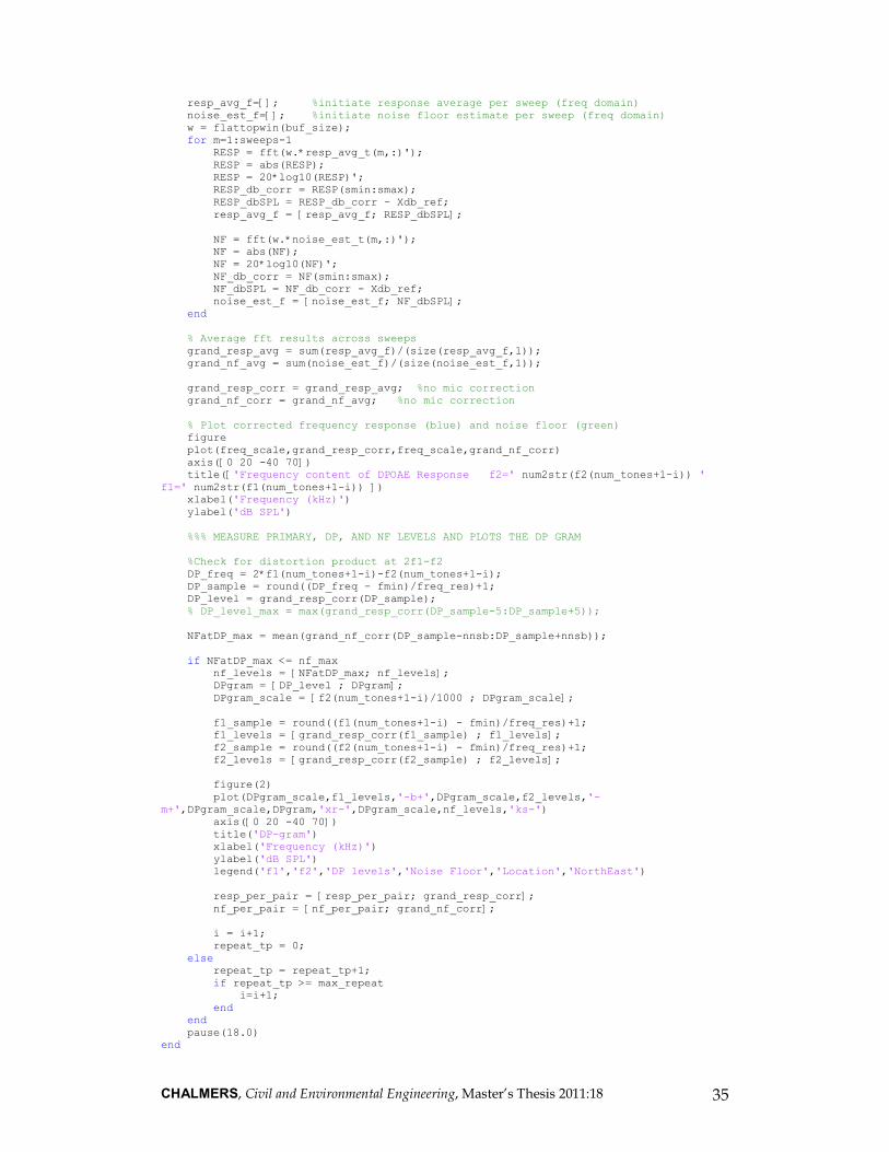
CHALMERS, Civil and Environmental Engineering, Master’s Thesis 2011:18 35
resp_avg_f=[]; %initiate response average per sweep (freq domain) noise_est_f=[]; %initiate noise floor estimate per sweep (freq domain) w = flattopwin(buf_size); for m=1:sweeps-1 RESP = fft(w.*resp_avg_t(m,:)'); RESP = abs(RESP); RESP = 20*log10(RESP)'; RESP_db_corr = RESP(smin:smax); RESP_dbSPL = RESP_db_corr - Xdb_ref; resp_avg_f = [resp_avg_f; RESP_dbSPL]; NF = fft(w.*noise_est_t(m,:)'); NF = abs(NF); NF = 20*log10(NF)'; NF_db_corr = NF(smin:smax); NF_dbSPL = NF_db_corr - Xdb_ref; noise_est_f = [noise_est_f; NF_dbSPL]; end % Average fft results across sweeps grand_resp_avg = sum(resp_avg_f)/(size(resp_avg_f,1)); grand_nf_avg = sum(noise_est_f)/(size(noise_est_f,1)); grand_resp_corr = grand_resp_avg; %no mic correction grand_nf_corr = grand_nf_avg; %no mic correction % Plot corrected frequency response (blue) and noise floor (green) figure plot(freq_scale,grand_resp_corr,freq_scale,grand_nf_corr) axis([0 20 -40 70]) title(['Frequency content of DPOAE Response f2=' num2str(f2(num_tones+1-i)) ' f1=' num2str(f1(num_tones+1-i)) ]) xlabel('Frequency (kHz)') ylabel('dB SPL') %%% MEASURE PRIMARY, DP, AND NF LEVELS AND PLOTS THE DP GRAM %Check for distortion product at 2f1-f2 DP_freq = 2*f1(num_tones+1-i)-f2(num_tones+1-i); DP_sample = round((DP_freq - fmin)/freq_res)+1; DP_level = grand_resp_corr(DP_sample); % DP_level_max = max(grand_resp_corr(DP_sample-5:DP_sample+5)); NFatDP_max = mean(grand_nf_corr(DP_sample-nnsb:DP_sample+nnsb)); if NFatDP_max <= nf_max nf_levels = [NFatDP_max; nf_levels]; DPgram = [DP_level ; DPgram]; DPgram_scale = [f2(num_tones+1-i)/1000 ; DPgram_scale]; f1_sample = round((f1(num_tones+1-i) - fmin)/freq_res)+1; f1_levels = [grand_resp_corr(f1_sample) ; f1_levels]; f2_sample = round((f2(num_tones+1-i) - fmin)/freq_res)+1; f2_levels = [grand_resp_corr(f2_sample) ; f2_levels]; figure(2) plot(DPgram_scale,f1_levels,'-b+',DPgram_scale,f2_levels,'-m+',DPgram_scale,DPgram,'xr-',DPgram_scale,nf_levels,'ks-') axis([0 20 -40 70]) title('DP-gram') xlabel('Frequency (kHz)') ylabel('dB SPL') legend('f1','f2','DP levels','Noise Floor','Location','NorthEast') resp_per_pair = [resp_per_pair; grand_resp_corr]; nf_per_pair = [nf_per_pair; grand_nf_corr]; i = i+1; repeat_tp = 0; else repeat_tp = repeat_tp+1; if repeat_tp >= max_repeat i=i+1; end end pause(18.0) end
CHALMERS, Civil and Environmental Engineering, Master’s Thesis 2011:18 36
%%% end while loop %%% %%% Save data with date-coded and sequential filenaming system %%% dataname = [cal_filename(1:end-4)]; iter = str2num(dataname(end-1:end)); checkfile=1; while checkfile if exist([dataname '.mat']) == 2 iter = iter+1; if iter < 10 dataname = [dataname(1:end-2) '0' num2str(iter)]; else dataname = [dataname(1:end-2) num2str(iter)]; end else checkfile = 0; end end bcu_MCL = str2num(get(findobj('tag','BCU_MCL'),'string')); bcu_th = str2num(get(findobj('tag','BCU_SL'),'string')); bcu_dBSL = str2num(get(findobj('tag','dB_mask'),'string')); save(dataname, 'cal_filename','f1','f2','L1_SPL','L2_SPL','L1_V','L2_V','Fs','sweeps','sets','buf_size','f2_f1_ratio','num_tones', ... 'freq_scale','resp_per_pair','nf_per_pair','DPgram_scale','DPgram','nf_levels','f1_levels','f2_levels','bcu_MCL','bcu_th','bcu_dBSL'); delete(ai) clear ai delete(ao1) clear ao1 delete(ao2) clear ao2

CHALMERS, Civil and Environmental Engineering, Master’s Thesis 2011:18 37
Appendix B Input Panel for DPOAE tests