Blind Source Separation with Conjugate Gradient Algorithm ...

Blind Source Separation with Conjugate Gradient Algorithm and Kurtosis

Maximization Criterion 1Sanjeev N Jain, 2Chandra Shekhar Rai

1Research Scholar Department of Electronics and Communication Engineering

S.J.J.T. University, Vidyanagar, Rajasthan- 333001 [email protected]

2Dean Department of Information and Technology

G.G.S.Indraprastha University, New Delhi - 110075

Abstract : Blind source separation (BSS) is a technique for estimating individual source components from their mixtures at multiple sensors. It is called blind because any additional other information will not be used besides the mixtures. Recently, blind source separation has received attention because of its potential applications in signal processing such as in speech recognition systems, telecommunications and medical signal processing. Blind source separation of super and sub-Gaussian Signal is proposed utilizing conjugate gradient algorithm and kurtosis maximization criteria. In our previous paper, ABC algorithm was utilized to blind source separation and here, we improve the technique with changes in fitness function and scout bee phase. Fitness function is improved with the use of kurtosis maximization criterion and scout bee phase is improved with use of conjugate gradient algorithm. The evaluation metrics used for performance evaluation are fitness function values and distance values. Comparative analysis is also carried out by comparing our proposed technique to other prominent techniques. The technique achieved average distance of 38.39, average fitness value of 6.94, average Gaussian distance of 58.60 and average Gaussian fitness as 5.02. The technique attained lowest average distance value among all techniques and good values for all other evaluation metrics which shows the effectiveness of the proposed technique.

Keywords:- Kurtosis Maximization, Conjugate Gradient Method, Blind Source Separation, Ant Bee Colony, Sub-Gaussian and Super-Gaussian signal.

I. INTRODUCTION

Blind source separation has received considerable attention among researchers as it has vast application and hasboth theoretical significance and practical importance [9]. A number of blind separation algorithms have been proposed based on different separation models [10]. Blind source separation is to recover unobservable independent sources from multiple observed data masked by linear or nonlinear mixing. In BSS, the source signals and the parameter of mixing model are unknown. The unknown original source signals can be separated and estimated using only the observed signals which are given through unobservable mixture [5]. Its numerous promising applications are in the areas of speech signal processing [1], [2], medical signal Processing including ECG, MEG, and EEG [3], and monitoring [9,13].The problem of source separation is to extract independent signals from their linear or nonlinear mixtures. So-called blind source separation (BSS) is to recover original source signals from their mixtures without any prior information on the sources themselves and the mixing parameters of the mixtures [11,14]. The algorithm is susceptible to the local minima problem during the learning process and is limited in many practical applications such as BSS that requires a global optimal solution [10, 12, 16].

Several techniques have been proposed in the literature for blind source separation that are mainly classified based on optimization algorithm [15, 17] and non-optimization algorithm [3-8] like genetic algorithm and particle swarm optimization for blind source separation. EM algorithm based techniques are employed. In our previous paper, ABC algorithm was utilized to blind source separation and here, we improve the technique with changes in fitness function and scout bee phase. Fitness function is improved with the use of kurtosis maximization criterion and scout bee phase is improved with use of conjugate gradient algorithm.The technique is composed of three modules, namely signal mixing module, weight matrix generation module and source separation module. The input source signals are combined and multiplied with a reference signal to have the mixed signal.From the mixed signal, we have to recover the source signals without having prior knowledge. This is accomplished by generating a weighting matrix by the use of Artificial Bee Colony with the aid of

e-ISSN : 0975-4024 Sanjeev N Jain et al. / International Journal of Engineering and Technology (IJET)

p-ISSN : 2319-8613 Vol 8 No 1 Feb-Mar 2016 64

conjugate gradient algorithm and kurtosis maximization criteria. This generated matrix is multiplied with the mixed matrix to obtain the estimated source matrix.

The rest of this paper is organized as follows. Section 2 gives a brief description of the related works and the proposed technique in detailed in section 3. The experimental analysis and discussions are presented in section 5 and section 6 gives the conclusion.

II. REVIEW OF RELATED WORKS

There has been several works in the literature associated with blind source separation. In this section, we discuss the some of those works. HamedModaghegh, SeyedAlirezaSeyedin [18] havepresented an active steganalysis method in order to break the block-discrete cosine transform (DCT) coefficients steganography. Their method was based on a combination of the Blind Source Separation (BSS) technique and Maximum A posteriori (MAP) estimator. Sawada et al. [1] have presented a blind source separation method for convolutive mixtures of speech/audio sources. Here, frequency-domain mixture samples were clustered into each source by an expectation–maximization (EM) algorithm. Duong et al. [2] have investigated the blind source separation performance stemming from rank-1 and full-rank models of the source spatial covariances. For that purpose, they addressed the estimation of model parameters by maximizing the likelihood of the observed mixture data using the EM algorithm with a proper initialization scheme.Reju, V.G. SooNqeeKohet al. [3] have proposed two algorithms, one for the estimation of the masks which were to be applied to the mixture in the TF domain for the separation of signals in the frequency domain, and the other for solving the permutation problem. The algorithm for mask estimation was based on the concept of angles in complex vector space. Diogo Cet al. [5] have presented a method to perform blind extraction of chaotic deterministic sources mixed with stochastic signals. This technique employed the recurrence quantification analysis (RQA), a tool commonly used to study dynamical systems, to obtain the separating system that recovers the deterministic source.

Takahataet al. [6] have reviewed some key aspects of two important branches in unsupervised signal processing: blind deconvolution and blind source separation (BSS). It also gave an overview of their potential application in seismic processing, with an emphasis on seismic deconvolution. Xiao-Feng Gong and Qiu-Hua Lin [7] have considered the problem of blind separation for convolutivespeech mixtures. The problem of permutation correction was solved in the method by simultaneously extracting and pairing two adjacent frequency responses, and exploiting the common factors shared by neighboring cross frequency covariance tensors. Sheng lixieet al. [8] have presented a time-frequency (TF) underdetermined blind source separation approach based on Wigner-Ville distribution (WVD) and Khatri-Rao product to separate N non-stationary sources from many mixtures. The improved method was proposed for estimating the mixing matrix, and after extracting all the auto-term TF points, the auto WVD value of the sources was found out.

III. PROPOSEDBLIND SOURCE SEPARATION WITH CONJUGATE GRADIENT ALGORITHM AND KURTOSIS

MAXIMIZATION CRITERION

Blind source separation (BSS) is a technique for estimating individual source components from their mixtures at multiple sensors without any additional other information. In this paper, blind source separation of super and sub-Gaussian Signalis proposed utilizing conjugate gradient algorithm and kurtosis maximization criteria. In our previous paper, ABC algorithm was utilized to blind source separation and here, we improve the technique with changes in fitness function and scout bee phase. Fitness function is improved with the use of kurtosis maximization criterion and scout bee phase is improved with use of conjugate gradient algorithm.

A. Signal Mixing Module

In this module, the input source signals are combined and multiplied with a reference signal to have the mixed signal. The block diagram of the module is given in figure 1.



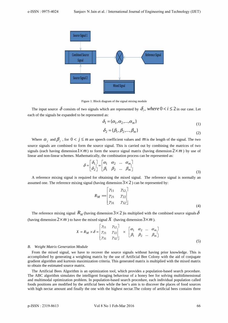
Figure 1: Block diagram of the signal mixing module

The input source δ consists of two signals which are represented by 20, ≤< iwhereiδ in our case. Let

each of the signals be expanded to be represented as:

},...,,{ 211 mαααδ =

(1)

},...,,{ 212 mβββδ = (2)

Where jα and jβ , for mj ≤<0 are speech coefficient values and m is the length of the signal. The two

source signals are combined to form the source signal. This is carried out by combining the matrices of two

signals (each having dimension m×1 ) to form the source signal matrix (having dimension m×2 ) by use of linear and non-linear schemes. Mathematically, the combination process can be represented as:

=

=

m

m

βα

ββαα

δδ

δ...

...

21

21

2

1

(3)

A reference mixing signal is required for obtaining the mixed signal. The reference signal is normally an

assumed one. The reference mixing signal (having dimension 23× ) can be represented by:

==

32

22

12

31

21

11

γγγ

γγγ

MR

(4)

The reference mixing signal MR (having dimension 23× )is multiplied with the combined source signalsδ

(having dimension m×2 ) to have the mixed signal X (having dimension m×3 ).

×

=×=

m

mMRX

βα

ββαα

γγγ

γγγ

δ...

...

21

21

32

22

12

31

21

11

(5)

B. Weight Matrix Generation Module

From the mixed signal, we have to recover the source signals without having prior knowledge. This is accomplished by generating a weighting matrix by the use of Artificial Bee Colony with the aid of conjugate gradient algorithm and kurtosis maximization criteria. This generated matrix is multiplied with the mixed matrix to obtain the estimated source matrix.

The Artificial Bees Algorithm is an optimization tool, which provides a population-based search procedure. The ABC algorithm simulates the intelligent foraging behaviour of a honey bee for solving multidimensional and multimodal optimization problem. In population-based search procedure, each individual population called foods positions are modified by the artificial bees while the bee’s aim is to discover the places of food sources with high nectar amount and finally the one with the highest nectar.The colony of artificial bees contains three



groups of bees: employed bees, onlookers and scouts. A bee waiting on the dance area for making decision to choose a food source is called an onlooker and a bee going to the food source visited by it previously, is named an employed bee. A bee carrying out random search is called a scout.

In each cycle, the search consists of three steps: sending the employed bees onto the food sources and then measuring their nectar amounts; selecting of the food sources by the onlookers after sharing the information of employed bees and determining the nectar amount of the foods; determining the scout bees and then sending them onto possible food sources. Here, the position of a food source represents a possible solution of the optimization problem and the nectar amount of a food source corresponds to the fitness of the associated solution. At the initialization stage, a set of food source positions are randomly selected by the employed bees and the population of the positions is subjected to repeated cycles of the search processes of the employed bees, the onlooker bees and scout bees. Provided that the nectar amount of the new source is higher than that of the previous one the bee memorizes the new position and forgets the old one. Otherwise she keeps the position of the previous one. Here, if a position cannot be improved further through a predetermined number of cycles called limit then that food source is assumed to be abandoned.

In our case, ABC is employed to find out the weight matrix so as to aid in the signal recovery. Initial matrix would be random which would be updated in each step with aid from the kurtosis fitness function and conjugate gradient based scout bee phase. The weighting matrix is of the size 32× and initially the colony is assumed to have six different matrices as the initial population. Let these initial population matrices be represented as:

][ 654321 PPPPPPP = (6)

Where each matrix iP is defined as:

61,232221

131211 ≤≤

= iPi ρρρ

ρρρ

(7)

Where )30,20(11 ≤<≤< jiρ are randomly generated values. The matrices are evaluated using the

kurtosis maximization criteria.

Kurtosis Maximization criteria based fitness function

Fitness functions are used to find the best matrices that would give best recovered output. In our case, we use kurtosis maximization based fitness function and entropy based fitness function. Kurtosis is any measure of the peakedness of the probability distribution of a real-valued random variable. One common measure of kurtosis is based on a scaled version of the fourth moment of the data or population. In our case, the weighting matrix is

multiplied with the mixed matrix to yield recovered signal *δ . Hence, it can be written such as:

XP×=*δ (8)

Let us define a matrix q which is the inverse of P matrix. The function is found out over arbitrary taken

G number of points. Then, the thg kurtosis value for the thi iteration is given by:

3})]()({[)( 4* −= iiqEikurt Tg δ

(9)

The thg kurtosis value for the thi iteration is given by:

= =

Δ∂

∂+=+

N

j

g

kj

j

kgg iq

iq

ikurtikurtikurt

1 1

)()(

)()()1(

(10)

Where )()1()( iqiqiq jjj −+=Δ . Equation 10 can be expanded using Taylor series to become:

)(][][4)()1( *3 iqDikurtikurt ii Δ++=+ δ (11)

Where,

=)()(...0

.........

0...)()(

][*

*1

iiq

iiq

D

GT

T

i

δ

δ.



Hence, kurtosis based fitness function has been defined and can be represented as kf . Suppose the entropy

of mixed signals is represented by )(iΓ , then the entropy based function ( ef ) can be defined by:

)(1

1

i

m

i

ef

Γ

=

= (12)

The combined fitness function is given by:

ek fffitness .. βα += (13)

The generated matrices are evaluated using this combined fitness function. Initially,best matrix from the initial six random generated matrices is found out and taken for further processing.

Employed bee and onlooker bee phase

In the initial phase, best matrix (represented by )B from the generated matrices was found out using the

fitness functions. In employed bee phase, the values of all the six matrices are changed with respect to the best matrix found out. The updation of the matrix is carried using the formula:

60)( ≤<−+= iforPBBV ii φ (14)

Where, iV is the updated value of initially taken iP matrix and φ is randomly produced number in the range

[-1,1] . The matrix updation is given by:

)(

)(

)(

)(

)(

)(

66

55

44

33

22

11

PBBV

PBBV

PBBV

PBBV

PBBV

PBBV

−+=−+=−+=−+=−+=−+=

φφφφφφ

(15)

Hence, all the matrices values are updated to obtain updated six matrices represented

by ].[ 654321 VVVVVVV = Best matrix among the updated matrices is found out using the fitness function

and is represented asC .

The best matrix obtained using the employed bee phase is again improved in the onlooker phase. Here, an element in the best matrix is replaced by an arbitrary value in the range [1,6] each time so as to result in six new

matrices. Suppose is C represented as:

=

232221

131211

ccc

cccC

Then six new matrices are given by:

=

=

=

=

=

=

232221

1312116

232221

1312115

232221

1312114

232221

1312113

232221

1312112

232221

1312111

,,

,,

σσσ

σσσ

cc

cccF

cc

cccF

cc

cccF

ccc

ccF

ccc

ccF

ccc

ccF

(16)

Hence, all the matrices values are updated to obtain updated six matrices represented

by ].[ 654321 FFFFFFF = Best matrix among the updated matrices is found out using the fitness function

and is represented as L .

Scout Bee Phase

Normally, in scout bee phase random matrices are generated but in our case, we employ conjugate gradient method for having better result. The conjugate gradient method is an algorithm for the numerical solution of particular systems of linear equations, namely those whose matrix is symmetric and positive-definite.



Consider the system XL×=*δ . Initially, residual at the thk step is found using the equation:

kk LXR −= *δ (17)

Then we have to find the direction kP given by:

001 ;0, RPiforPRP kkkk =>+= −β (18)

Where, scalar constants are given by the equations:

kTk

kkk

PLP

PLR 1+−=β

(19)

kT

k

kT

kk

LPP

RR=α

(20)

New kX is computed as:

111 −−+ += kkkk PXX α (21)

The process is continued for certain number of iterations to yield new matrix. This entire process is carried out for all six onlooker bee phase matrix outputs to generate new six matrix represented by

].[ 654321 UUUUUUU =

Hence, in a single iteration we obtain 24 matrices and form these 24, the best six matrices are chosen using fitness function value and given as input to the next iteration. This six would act as the initially generated matrices in the iteration. The same process of employed bee, onlooker bee phase and scout bee phase is continued until the user required threshold is reached. The best matrices after all the iterations are taken as the final weight matrixψ .

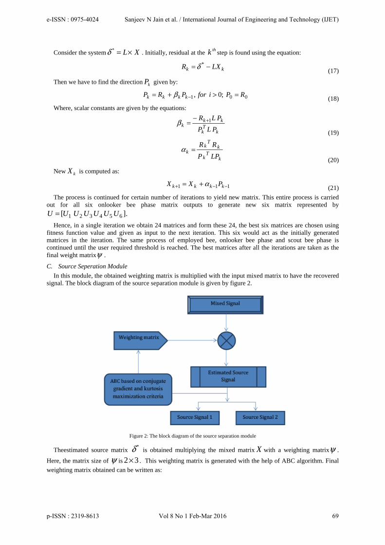
C. Source Seperation Module

In this module, the obtained weighting matrix is multiplied with the input mixed matrix to have the recovered signal. The block diagram of the source separation module is given by figure 2.

Figure 2: The block diagram of the source separation module

Theestimated source matrix *δ is obtained multiplying the mixed matrix X with a weighting matrixψ .

Here, the matrix size of ψ is 32× . This weighting matrix is generated with the help of ABC algorithm. Final

weighting matrix obtained can be written as:



=

23

13

2221

1211

λλ

λλλλ

ψ (22)

Recovered signal can be given by:

×

×

=×=

m

mXβα

ββαα

γγγ

γγγ

λλ

λλλλ

ψδ...

...

21

21

32

22

12

31

21

11

23

13

2221

1211*

(23)

Hence, signal has been recovered by the proposed technique.

IV. RESULTS AND DISCUSSIONS

In this section, results and discussions for the proposed blind source separation are given and analysed. Comparative analysis is also made by comparing to other existing techniques. In section 4.1, experimental set up and database details are given and in section 4.2 evaluation metric details are given. Simulation plots are given in section 4.3 and detailed analysis is given in section 4.4.

A. Experimental set up and evaluation metrics employed

The proposed technique for signal separation is implemented in MATLAB on a system having 6 GB RAM with 64 bit operating system having i7 Intel Processor. The evaluation metrics used for performance evaluation are fitness function values and distance values. Final function values contains both normal and that of Gaussian, similarly distance includes sound distance and Gaussian distance. Distance measure provides the distance between the original signal and the extracted signal through blind source separation.

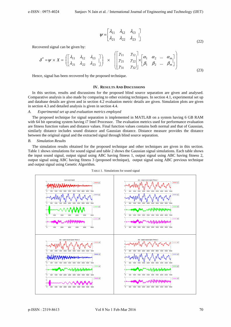
B. Simulation Results

The simulation results obtained for the proposed technique and other techniques are given in this section. Table 1 shows simulations for sound signal and table 2 shows the Gaussian signal simulations. Each table shows the input sound signal, output signal using ABC having fitness 1, output signal using ABC having fitness 2, output signal using ABC having fitness 3 (proposed technique), output signal using ABC previous technique and output signal using Genetic Algorithm.

TABLE 1. Simulations for sound signal



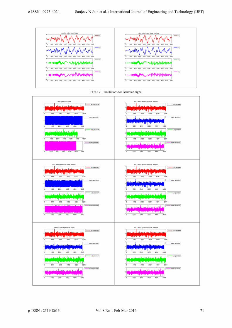
TABLE 2. Simulations for Gaussian signal



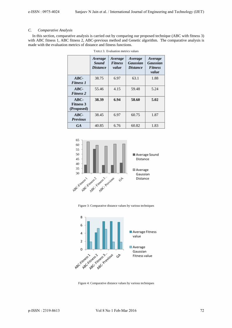
C. Comparative Analysis

In this section, comparative analysis is carried out by comparing our proposed technique (ABC with fitness 3) with ABC fitness 1, ABC fitness 2, ABC-previous method and Genetic algorithm. The comparative analysis is made with the evaluation metrics of distance and fitness functions.

TABLE 3. Evaluation metrics values

Average Sound

Distance

Average Fitness value

Average Gaussian Distance

Average Gaussian Fitness value

ABC-Fitness 1

38.75 6.97 63.1 1.88

ABC-Fitness 2

55.46 4.15 59.48 5.24

ABC- Fitness 3

(Proposed)

38.39 6.94 58.60 5.02

ABC- Previous

38.45 6.97 60.75 1.87

GA 40.85 6.76 60.82 1.83

30

35

40

45

50

55

60

65

Average Sound Distance

Average Gaussian Distance

Figure 3: Comparative distance values by various techniques

0

2

4

6

8

Average Fitness value

Average Gaussian Fitness value

Figure 4: Comparative distance values by various techniques



Inferences from tables 3 and figures 3 and 4:The comparative analysis is made with the evaluation metrics of sound distance, Gaussian distance, fitness functions and Gaussian fitness functions.

• Comparative analysis is carried out by comparing our proposed technique (ABC with fitness 3) with ABC fitness 1, ABC fitness 2, ABC-previous method and Genetic algorithm.

• Table 3 gives the evaluation metrics values. Figure 3 gives the comparative distance values by various techniques and figure 4 gives the comparative distance values by various techniques.

• From the results, we can observe that our proposed technique has obtained good results by obtaining low distance metrics and high fitness values.

• The technique obtained average distance of 38.39, average fitness value of 6.94, average Gaussian distance of 58.60 and average Gaussian fitness as 5.02.

• The technique yielded lowest distance among all techniques and good values for all other evaluation metrics which shows the effectiveness of the proposed technique.

V. CONCLUSION

In this paper, blind source separation of super and sub-Gaussian Signal is proposed utilizing conjugate gradient algorithm and kurtosis maximization criteria. The technique is composed of three modules, namely signal mixing module, weight matrix generation module and source separation module.The evaluation metrics used for performance evaluation are fitness function values and distance values. Comparative analysis is also carried out by comparing our proposed technique to other prominent techniques. The technique achieved average distance of 38.39, average fitness value of 6.94, average Gaussian distance of 58.60 and average Gaussian fitness as 5.02. The technique attained lowest average distance value among all techniques and good values for all other evaluation metrics which shows the effectiveness of the proposed technique.

REFERENCE [1] Sawada, H.Araki, Makino,"Underdetermined Convolutive Blind Source Separation via Frequency Bin-Wise Clustering and

Permutation Alignment", IEEE transaction on Audio, Speech, and Language Processing, vol.19, pp.516-527, 2011. [2] Duong, Vincent, Gribonval, "Under-determined convolutive blind source separation using spatial covariance models", IEEE

International Conference on Acoustics Speech and Signal Processing (ICASSP), pp.9-12, 2010. [3] Reju, V.G. SooNqeeKoh, "Underdetermined Convolutive Blind Source Separation via Time–Frequency Masking", IEEE Transactions

on Audio, Speech, and Language Processing, vol.18, pp.101-116, 2010. [4] F. Rojas, C.G. Puntonet, J.M. Gorriz, and O. Valenzuela, "Assessing the Performance of Several Fitness Functions in a Genetic

Algorithm for Nonlinear Separation of Sources", LNCS, pp. 863–872, 2005. [5] Diogo C. Sorianoa, Ricardo Suyamab, RomisAttux, "Blind extraction of chaotic sources from mixtures with stochastic signals based

on recurrence quantification analysis", conference on Digital Signal Processing, Volume 21, pp.417–426, 2011. [6] Takahata, Nadalin, Ferrari, Duarte, Suyama, Lopes, Romano, Tygel, "Unsupervised Processing of Geophysical Signals: A Review of

Some Key Aspects of Blind Deconvolution and Blind Source Separation", IEEE transaction on Signal Processing Magazine, Volume: 29, pp. 27-35, 2012.

[7] Xiao-Feng Gong and Qiu-HuaLin,"Speech Separation via Parallel Factor Analysis of Cross-Frequency Covariance Tensor", Latent Variable Analysis and Signal Separation, Vol.6365, pp. 65-72, 2010.

[8] Sheng lixie ,Liu Yang , Jun-Mei Yang , Guoxu Zhou , Yong Xiang, “Time-Frequency Approach To Underdetermined Blind Source Separation,”IEEE transaction on Neural Networks and Learning Systems, vol.23 , pp. 306 - 316 , 2012.

[9] Ying Tan, Jun Wang, Jacek M. Zurada, “Nonlinear Blind Source Separation Using A Radial Basis Function Network,” IEEE Transactions On Neural Networks, Vol. 12, 2001.

[10] F.Rojas, I.Rojas, R.M.Clemente, C.G.Puntonet, “Nonlinear Blind Source Separation Using Genetic Algorithms,” 2002. [11] Harrivalpola, ErkkiOja, Alexander Ilin, AnttiHonkela, JuhaKarhunen,” Nonlinear Blind Source Separation by Variational Bayesian

Learning,” IEICE Transaction, VOL.82, 1999. [12] Samira Mavaddaty and AtaollahEbrahimzadeh,”Blind Signals Separation with Genetic Algorithm and Particle Swarm Optimization

Based on Mutual Information”, Radioeletronics and communications Systems,Vol.54, No.6, pp.315-324, 2011. [13] Samira Mavaddaty and AtaollahEbrahimzadeh, “Blind Signals Separation with Genetic Algorithm and Particle Swarm Optimization

Based on Mutual Information”, Radio-eletronics and communications Systems, Vol.54, No.6, pp.315-324, 2011. [14] Frederic Abrard, Yannick Deville, “A time–frequency blind signal separation method applicable to underdetermined mixtures of

dependent sources”, conference on signal processing,Vol. 85, PP. 1389–1403, 2005. [15] Samira Mavaddaty, AtaollahEbrahimzadeh, "Research of Blind Signals Separation with Genetic Algorithm and Particle Swarm

Optimization Based on Mutual Information", Radioelectron.Commun.Syst, Vol. 54, No. 6, pp. 315–324, 2011. [16] Ran Chen and Wen-Pei Sung, "Nonlinear Blind Source Separation Using GA Optimized RBF-ICA and its Application to the Image

Noise Removal", Advanced Materials Research, pp.205-208, 2011. [17] Gonzalez, E.A. Goorriz, J.M. ; Ramrrez, J. ; Puntonet, C.G. , "Elitist genetic algorithm guided by higher order statistic for blind

separation of digital signals", IECON 2010 - 36th Annual Conference on IEEE Industrial Electronics Society, pp. 1123-1128, 2010. [18] HamedModaghegh, SeyedAlirezaSeyedin, "A new fast and efficient active steganalysis based on combined geometrical blind source

separation", Multimedia Tools and Applications, pp. 1380-7501, 2014.



Author Biographies

Mr. SANJEEV NATAVAR JAIN received the B.E. degree from the Shivaji University, Maharashtra, India in 1990, the M.E. degree from the D.A.V.V. University, Indore, Madhya Pradesh, India, in 1994. He is currently pursuing Phd at SJJT University, Rajasthan.. His research interests are in Solid State Devices, Wireless Sensor Networks, and Biomedical Signal Processing. He has some publications in International journals and conferences.

Dr. Chandra Shekhar Rai is a Professor with the University School of Information Technology since September, 2011. He served the University as Associate Professor from 2007 to 2011 and Reader from 2004 to 2007. He was lecturer with the same School from 1999 to 2004. He obtained his M.E. degree in Computer Engineering from SGS Institute of Technology & Science, Indore in 1994 and completed Ph.D. in area of Neural Network from Guru Gobind Singh Indraprastha University in 2003. He has earlier worked as a lecturer at Guru Jambeshwar University, Hissar. He has many publications in International/national journals and conferences. He was conferred with “Best Teacher Award” of the University for the academic year 2007-2008 and second best researcher award of the University in the area of engineering and technology in 2010. He was Chairman, University Center for IT Services & Infrastructure Management (UCITIM) from 2007 to 2012. His teaching and research interests include: Artificial Neural Systems, Computer Networks and, Signal Processing.



Blind Source Separation with Conjugate Gradient Algorithm ...

Documents

Transcript of Blind Source Separation with Conjugate Gradient Algorithm ...