Bellringer 1 Explain in complete sentences what are world supply and demands of coal.
Upload
gwendoline-carrCategory
view
226download
0
BELLRINGER
1
EXPLAIN IN COMPLETE SENTENCES
OF RADAR WORK
2
Introduction to Radar Systems
3
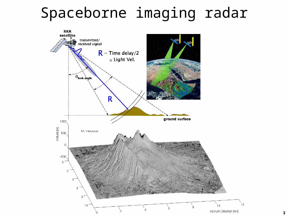
Spaceborne imaging radar
4
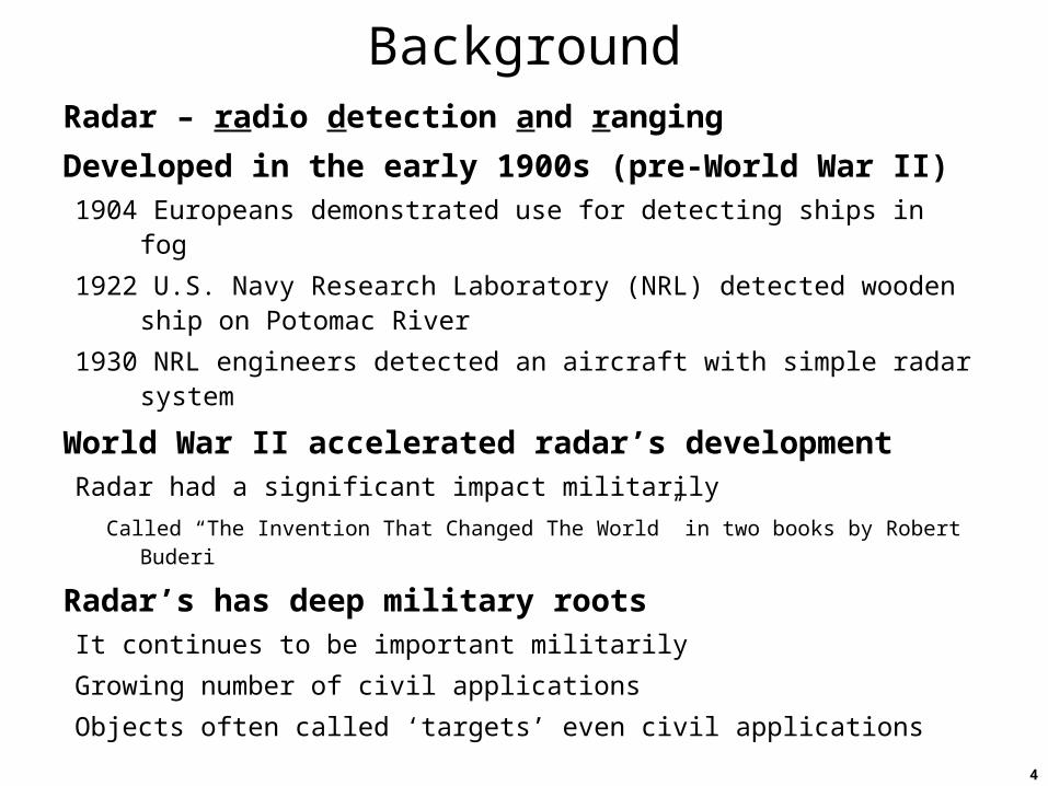
BackgroundRadar – radio detection and ranging
Developed in the early 1900s (pre-World War II)1904 Europeans demonstrated use for detecting ships in fog
1922 U.S. Navy Research Laboratory (NRL) detected wooden ship on Potomac River
1930 NRL engineers detected an aircraft with simple radar system
World War II accelerated radar’s developmentRadar had a significant impact militarily
Called “The Invention That Changed The World” in two books by Robert Buderi
Radar’s has deep military rootsIt continues to be important militarily
Growing number of civil applications
Objects often called ‘targets’ even civil applications
5
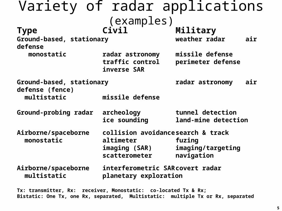
Variety of radar applications (examples)
Type Civil MilitaryGround-based, stationary weather radar air defense monostatic radar astronomy missile defense
traffic control perimeter defenseinverse SAR
Ground-based, stationary radar astronomy air defense (fence) multistatic missile defense
Ground-probing radar archeology tunnel detectionice sounding land-mine detection
Airborne/spaceborne collision avoidance search & track monostatic altimeter fuzing
imaging (SAR) imaging/targetingscatterometer navigation
Airborne/spaceborne interferometric SAR covert radar multistatic planetary exploration
Tx: transmitter, Rx: receiver, Monostatic: co-located Tx & Rx;Bistatic: One Tx, one Rx, separated, Multistatic: multiple Tx or Rx, separated
6
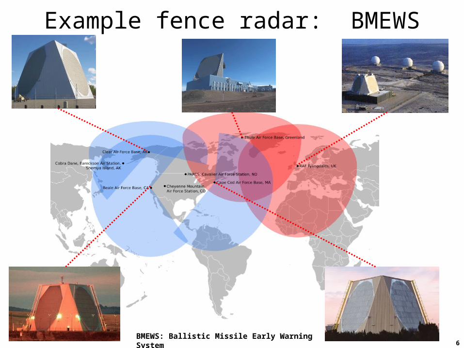
Example fence radar: BMEWS
BMEWS: Ballistic Missile Early Warning System
7
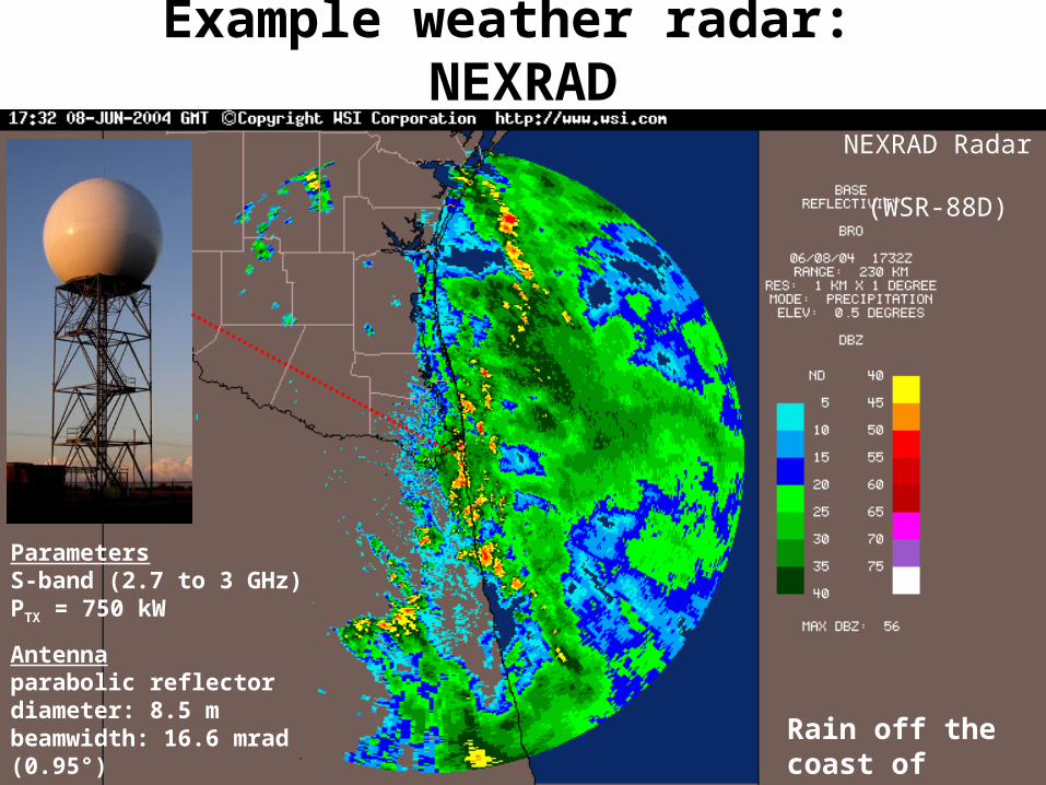
Example weather radar: NEXRAD
Rain off the coast of Brownsville, Texas
ParametersS-band (2.7 to 3 GHz)PTX = 750 kW
Antennaparabolic reflector diameter: 8.5 mbeamwidth: 16.6 mrad (0.95°)
NEXRAD Radar (WSR-88D)
8
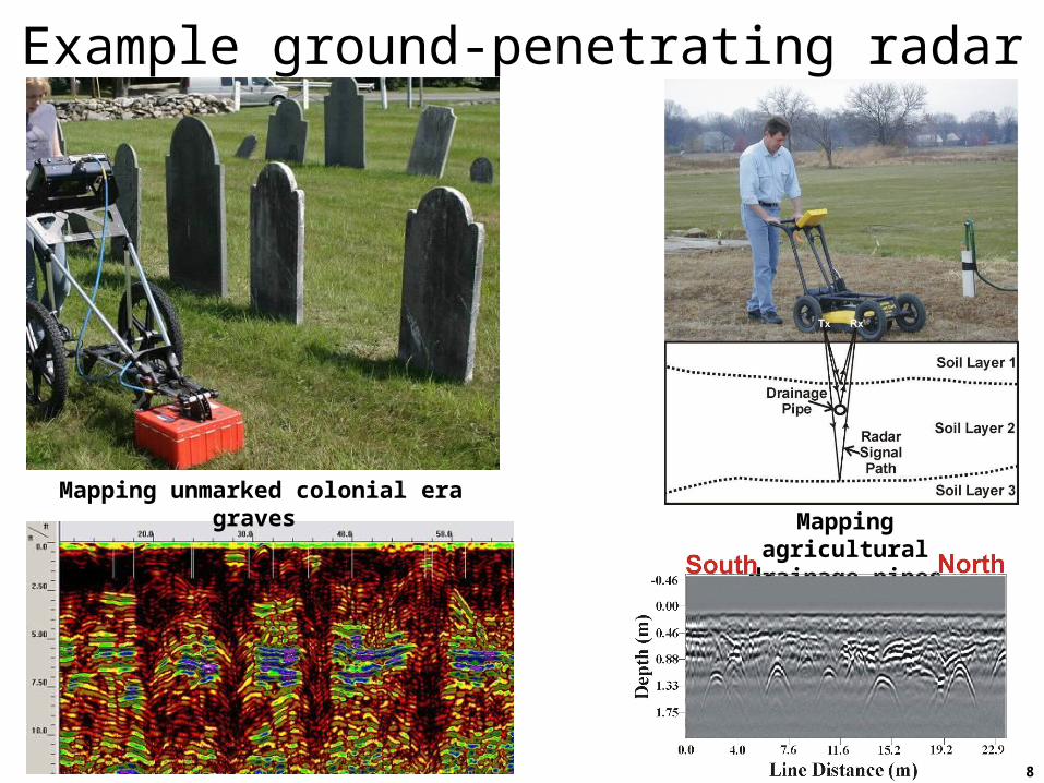
Example ground-penetrating radar
Mapping agricultural drainage pipes
Mapping unmarked colonial era graves
9
Characteristics of radarUses electromagnetic (EM) waves
Frequencies in the MHz, GHz, THz
Governed by Maxwell’s equations
Propagates at the speed of light
Antennas or optics used to launch/receive waves
Related technologies use acoustic waves
Ultrasound, seismics, sonar
Microphones, accelerometers, hydrophones used as transducers
Active sensorProvides its own illumination
Involves both a transmitter and a receiver
Related technologies are purely passive
Radio astronomy, radiometers
10
Concepts and technologies used in radarRadars are systems involving a wide range of technologies and concepts
An understanding of radar requires knowledge over this broad range of technologies and concepts
As new technologies emerge and new concepts are developed, radar capabilities can grow and improve
New enabling technologies signify breakthroughs
11
Concepts and technologies used in radarElectromagnetics
Antennas (multiple roles)• Impedance transformation (free-space intrinsic impedance to
transmission-line characteristic impedance)• Propagation mode adapter (free-space fields to guided waves)• Spatial filter (radiation pattern – direction-dependent sensitivity)• Polarization filter (polarization-dependent sensitivity)• Phase center• Arrays
Calibration targets (enhanced radar cross section RCS)• Passive (trihedral, sphere, Luneberg lens)• Active• Coded (time, amplitude, frequency, phase, polarization)
RCS suppression (stealth)Reflection, refraction, diffraction, propagation, absorption, dispersion
12
Concepts and technologies used in radarElectromagnetics
Scattering• Objects (shape, composition, orientation)• Surface (specular, facets, Bragg resonance, Kirchhoff scattering,
small-perturbation)• Volume (Rayleigh, Mie)
Materials (permittivity, permeability, conductivity) • Absorber• Radome
Doppler shiftCoherence and interference
• Fading• Fresnel zones
Numerical modeling, simulation, inversion• Finite difference time domain (FDTD)• Commercial CAD tools (HFSS, CST)
EM compatibility (emission, conduction, interference, susceptibility)
13
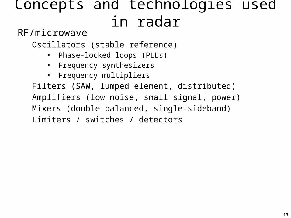
Concepts and technologies used in radarRF/microwave
Oscillators (stable reference)• Phase-locked loops (PLLs)• Frequency synthesizers• Frequency multipliers
Filters (SAW, lumped element, distributed)Amplifiers (low noise, small signal, power)Mixers (double balanced, single-sideband)Limiters / switches / detectors
ACTIVITY
14
DRAW THE FIGURE SHOWING HOW
THE RADAR CAN BE USED TO TRACK
SEVERE WEATHER AND THUNDERSTORMS
15
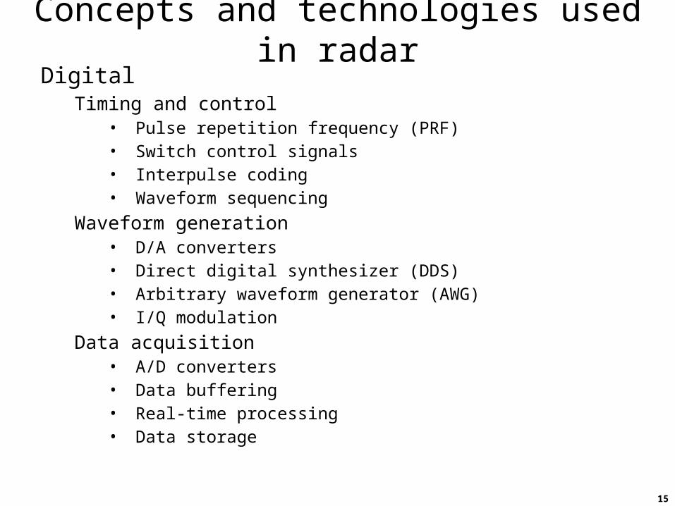
Concepts and technologies used in radarDigital
Timing and control• Pulse repetition frequency (PRF)• Switch control signals• Interpulse coding• Waveform sequencing
Waveform generation• D/A converters• Direct digital synthesizer (DDS)• Arbitrary waveform generator (AWG)• I/Q modulation
Data acquisition• A/D converters• Data buffering• Real-time processing• Data storage
16
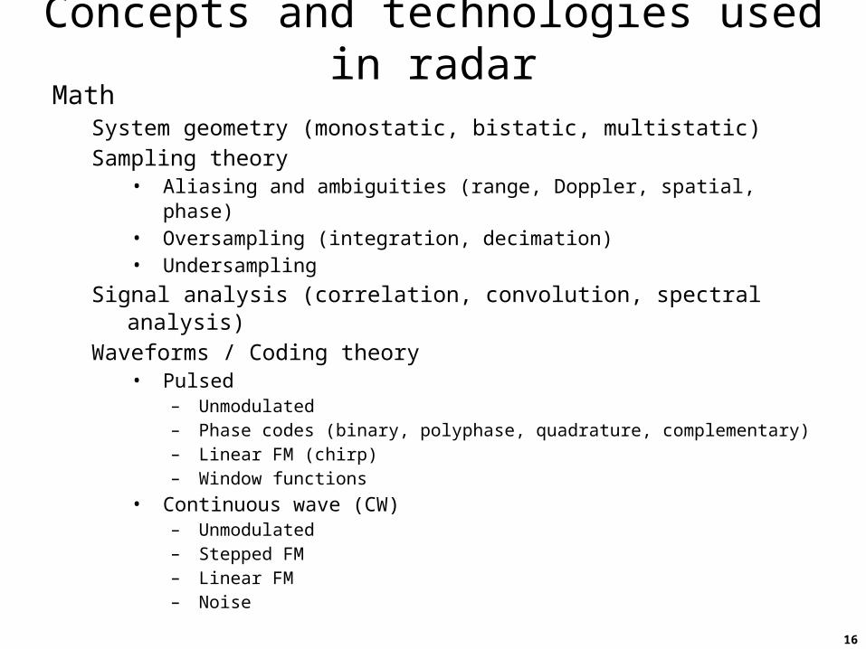
Concepts and technologies used in radarMath
System geometry (monostatic, bistatic, multistatic)Sampling theory
• Aliasing and ambiguities (range, Doppler, spatial, phase)• Oversampling (integration, decimation)• Undersampling
Signal analysis (correlation, convolution, spectral analysis)Waveforms / Coding theory
• Pulsed– Unmodulated– Phase codes (binary, polyphase, quadrature, complementary)– Linear FM (chirp)– Window functions
• Continuous wave (CW)– Unmodulated– Stepped FM– Linear FM– Noise
17
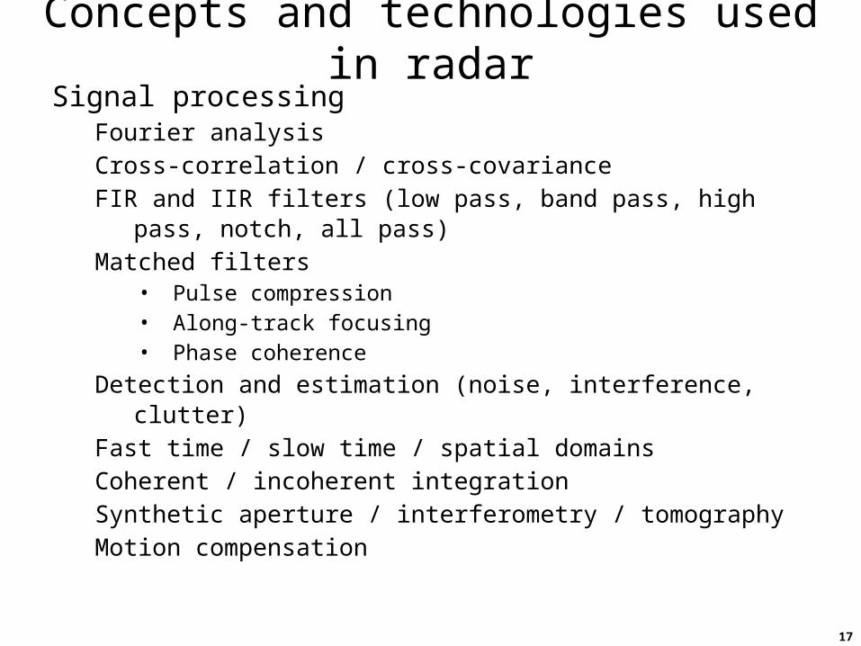
Concepts and technologies used in radarSignal processing
Fourier analysisCross-correlation / cross-covarianceFIR and IIR filters (low pass, band pass, high pass, notch, all pass)Matched filters
• Pulse compression• Along-track focusing• Phase coherence
Detection and estimation (noise, interference, clutter)Fast time / slow time / spatial domainsCoherent / incoherent integrationSynthetic aperture / interferometry / tomographyMotion compensation
18
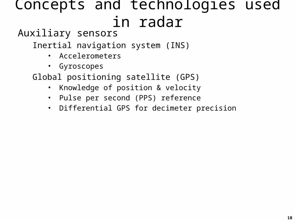
Concepts and technologies used in radarAuxiliary sensors
Inertial navigation system (INS)• Accelerometers• Gyroscopes
Global positioning satellite (GPS)• Knowledge of position & velocity• Pulse per second (PPS) reference• Differential GPS for decimeter precision
19
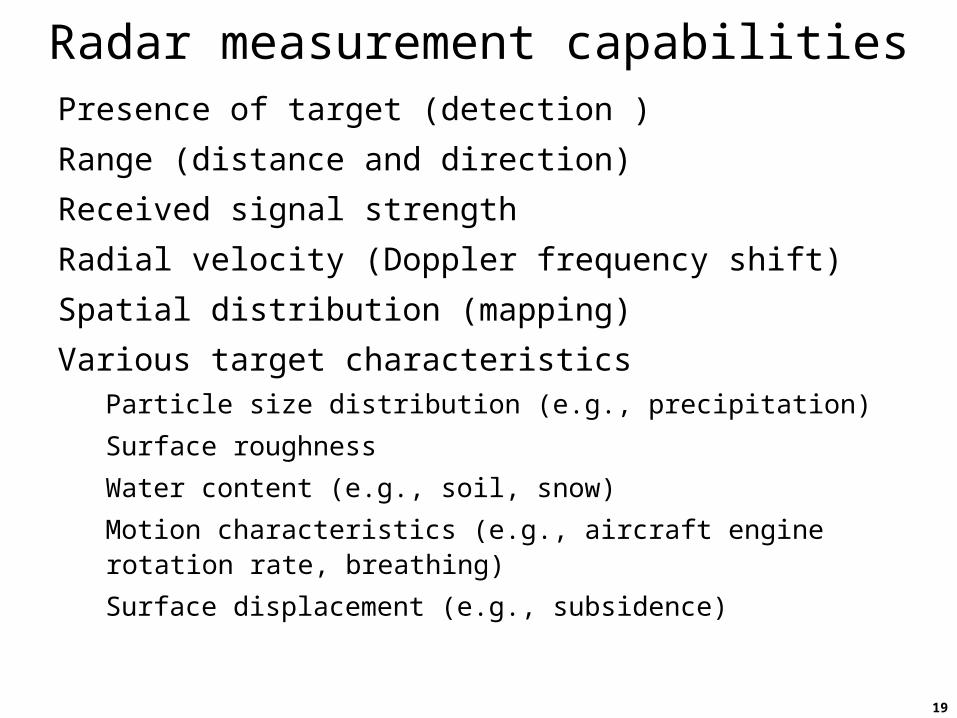
Radar measurement capabilitiesPresence of target (detection )
Range (distance and direction)
Received signal strength
Radial velocity (Doppler frequency shift)
Spatial distribution (mapping)
Various target characteristicsParticle size distribution (e.g., precipitation)
Surface roughness
Water content (e.g., soil, snow)
Motion characteristics (e.g., aircraft engine rotation rate, breathing)
Surface displacement (e.g., subsidence)
20
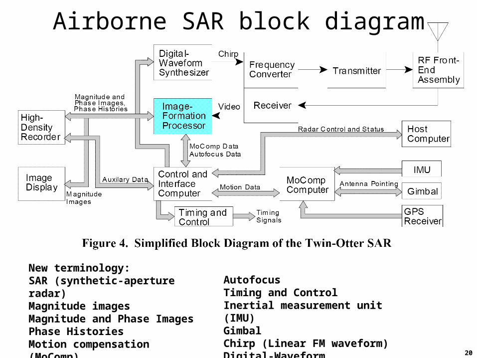
Airborne SAR block diagram
New terminology:SAR (synthetic-aperture radar)Magnitude imagesMagnitude and Phase ImagesPhase HistoriesMotion compensation (MoComp)Autofocus
AutofocusTiming and ControlInertial measurement unit (IMU)GimbalChirp (Linear FM waveform)Digital-Waveform Synthesizer
21
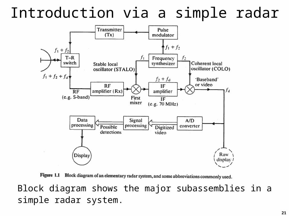
Introduction via a simple radar
Block diagram shows the major subassemblies in a simple radar system.
22
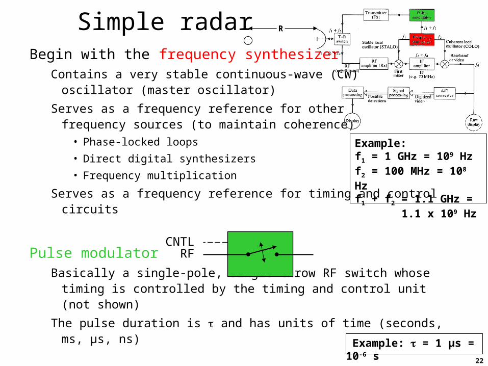
Simple radarBegin with the frequency synthesizer
Contains a very stable continuous-wave (CW)oscillator (master oscillator)
Serves as a frequency reference for otherfrequency sources (to maintain coherence)
• Phase-locked loops
• Direct digital synthesizers
• Frequency multiplication
Serves as a frequency reference for timing and control circuits
Pulse modulatorBasically a single-pole, single-throw RF switch whose timing is
controlled by the timing and control unit (not shown)
The pulse duration is and has units of time (seconds, ms, μs, ns)
CNTLRF
Example: = 1 μs = 10-6 s
Example:f1 = 1 GHz = 109 Hzf2 = 100 MHz = 108 Hzf1 + f2 = 1.1 GHz =
1.1 x 10⁹ Hz
R
23
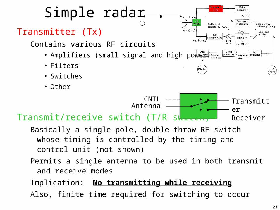
Simple radarTransmitter (Tx)
Contains various RF circuits• Amplifiers (small signal and high power)
• Filters
• Switches
• Other
Transmit/receive switch (T/R switch)Basically a single-pole, double-throw RF switch whose timing is
controlled by the timing and control unit (not shown)
Permits a single antenna to be used in both transmit and receive modes
Implication: No transmitting while receiving
Also, finite time required for switching to occur
CNTLAntenna
TransmitterReceiver
R
24
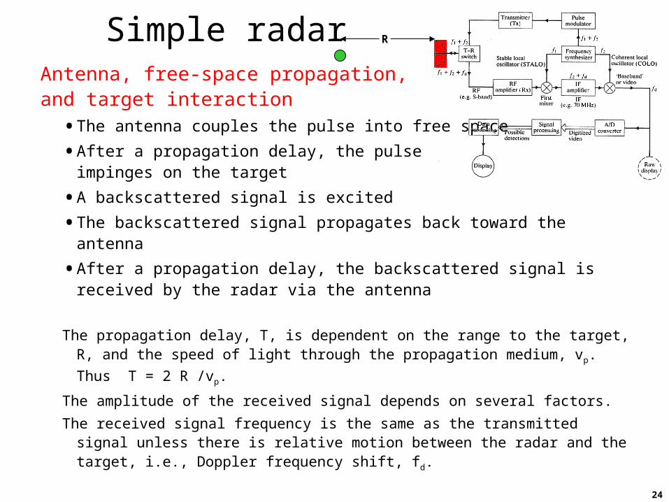
Simple radarAntenna, free-space propagation, and target interaction
• The antenna couples the pulse into free space
• After a propagation delay, the pulse impinges on the target
• A backscattered signal is excited
• The backscattered signal propagates back toward the antenna
• After a propagation delay, the backscattered signal is received by the radar via the antenna
The propagation delay, T, is dependent on the range to the target, R, and the speed of light through the propagation medium, vp. Thus T = 2 R /vp.
The amplitude of the received signal depends on several factors.
The received signal frequency is the same as the transmitted signal unless there is relative motion between the radar and the target, i.e., Doppler frequency shift, fd.
R
25
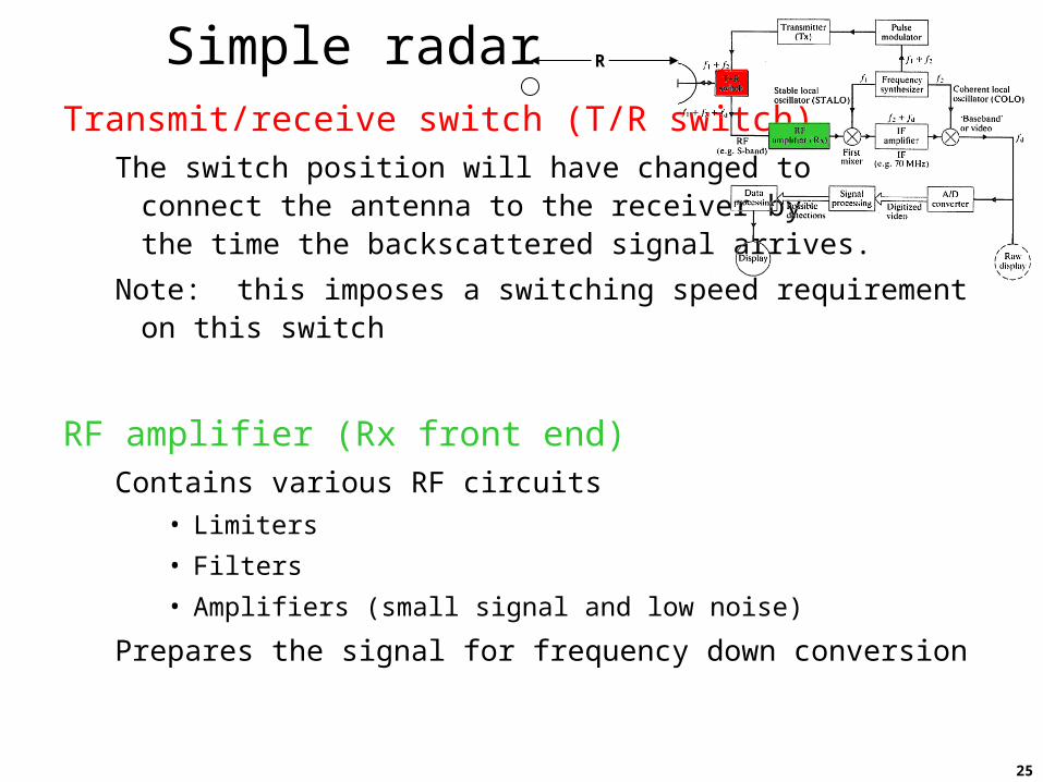
Simple radarTransmit/receive switch (T/R switch)
The switch position will have changed to connect the antenna to the receiver by the time the backscattered signal arrives.
Note: this imposes a switching speed requirement on this switch
RF amplifier (Rx front end)Contains various RF circuits
• Limiters
• Filters
• Amplifiers (small signal and low noise)
Prepares the signal for frequency down conversion
R
26
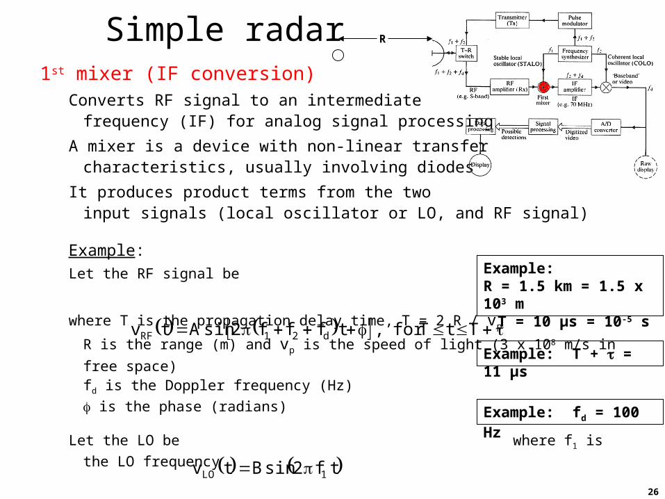
Simple radar1st mixer (IF conversion)
Converts RF signal to an intermediate frequency (IF) for analog signal processing
A mixer is a device with non-linear transfercharacteristics, usually involving diodes
It produces product terms from the two input signals (local oscillator or LO, and RF signal)
Example:
Let the RF signal be
where T is the propagation delay time, T = 2 R / vp
R is the range (m) and vp is the speed of light (3 x 10⁸ m/s in free space)
fd is the Doppler frequency (Hz)
is the phase (radians)
Let the LO be where f1 is the LO frequency
TtTfor,tfff2sinAtv d21RF
tf2sinBtv 1LO
Example:R = 1.5 km = 1.5 x 10³ m
T = 10 μs = 10-5 s
R
Example: fd = 100 Hz
Example: T + = 11 μs
27
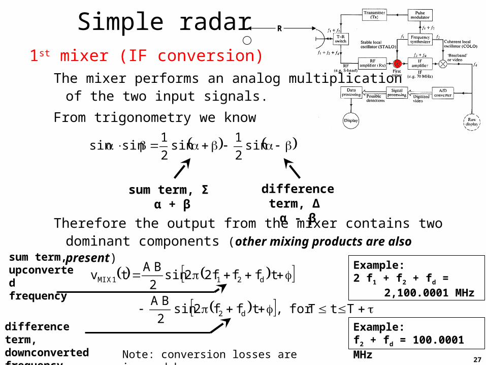
Simple radar1st mixer (IF conversion)
The mixer performs an analog multiplication of the two input signals.
From trigonometry we know
Therefore the output from the mixer contains two dominant components (other mixing products are also present)
TtTfor,tff2sin2
BA
tfff22sin2
BAtv
d2
d211MIX
sin2
1sin
2
1sinsin
sum term, Σ α + β
difference term, Δ α - β
sum term,upconverted
frequency
difference term, downconvertedfrequency Note: conversion losses are ignored here
R
Example:2 f1 + f2 + fd =
2,100.0001 MHz
Example:f2 + fd = 100.0001 MHz
28
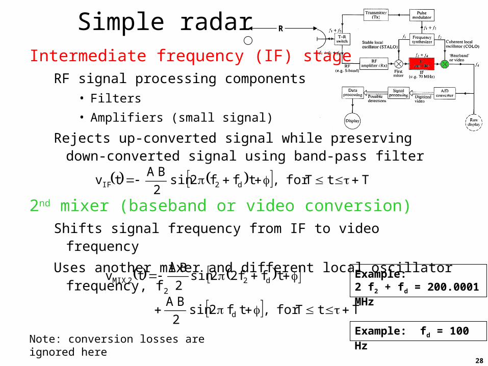
Simple radarIntermediate frequency (IF) stage
RF signal processing components• Filters
• Amplifiers (small signal)
Rejects up-converted signal while preserving down-converted signal using band-pass filter
2nd mixer (baseband or video conversion)Shifts signal frequency from IF to video frequency
Uses another mixer and different local oscillator frequency, f2
TtTfor,tff2sin2
BAtv d2IF
TtTfor,tf2sin2
BA
tff22sin2
BAtv
d
d22MIX
Note: conversion losses are ignored here
R
Example:2 f2 + fd = 200.0001 MHz
Example: fd = 100 Hz
29
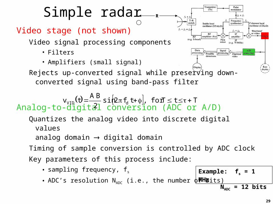
Simple radarVideo stage (not shown)
Video signal processing components• Filters
• Amplifiers (small signal)
Rejects up-converted signal while preserving down-converted signal using band-pass filter
Analog-to-digital conversion (ADC or A/D)Quantizes the analog video into discrete digital values
analog domain digital domain
Timing of sample conversion is controlled by ADC clock
Key parameters of this process include:
• sampling frequency, fs
• ADC’s resolution NADC (i.e., the number of bits)
TtTfor,tf2sin2
BAtv dVID
R
Example: fs = 1 MHzNADC = 12 bits
30
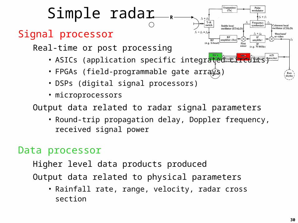
Simple radarSignal processor
Real-time or post processing• ASICs (application specific integrated circuits)
• FPGAs (field-programmable gate arrays)
• DSPs (digital signal processors)
• microprocessors
Output data related to radar signal parameters• Round-trip propagation delay, Doppler frequency, received signal
power
Data processorHigher level data products produced
Output data related to physical parameters• Rainfall rate, range, velocity, radar cross section
R
31
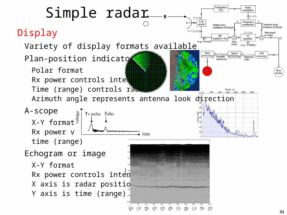
Simple radarDisplay
Variety of display formats available
Plan-position indicator (PPI)
Polar formatRx power controls intensity Time (range) controls radiusAzimuth angle represents antenna look direction
A-scope
X-Y formatRx power vs time (range)
Echogram or image
X-Y formatRx power controls intensityX axis is radar positionY axis is time (range)
R
32
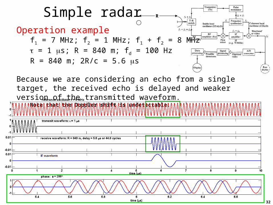
Simple radarOperation example
f1 = 7 MHz; f2 = 1 MHz; f1 + f2 = 8 MHz = 1 s; R = 840 m; fd = 100 HzR = 840 m; 2R/c = 5.6 s
Because we are considering an echo from a single target, the received echo is delayed and weaker version of the transmitted waveform.
Note that the Doppler shift is undetectable.
R

33
Simple radarSimple radar example
This example illustrates the basic features of a coherent, monostatic, pulse radar.
Coherent – all frequencies derived from central stable oscillator, signal phase preserved throughout
Monostatic – co-located Tx and Rx (in fact it shared a common antenna)
Pulse mode – pulsed waveform
Many variations are possibleNot all systems will require dual-stage frequency down-conversion
(the mixers)
Some systems will use waveforms more complex than a time-gated sinusoid
Some systems operate in continuous-wave (CW) mode rather than pulsed
R
34
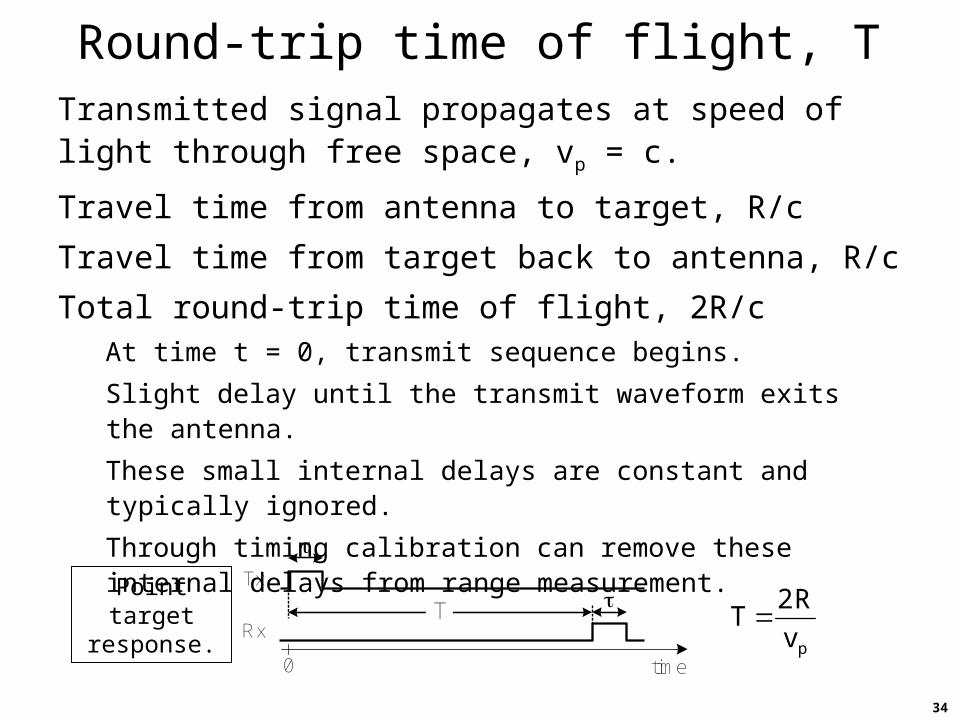
Round-trip time of flight, TTransmitted signal propagates at speed of light through free space, vp = c.
Travel time from antenna to target, R/c
Travel time from target back to antenna, R/c
Total round-trip time of flight, 2R/cAt time t = 0, transmit sequence begins.
Slight delay until the transmit waveform exits the antenna.
These small internal delays are constant and typically ignored.
Through timing calibration can remove these internal delays from range measurement.
T.
time
Tx
Rx
0
Point target response.
pv
R2T
35
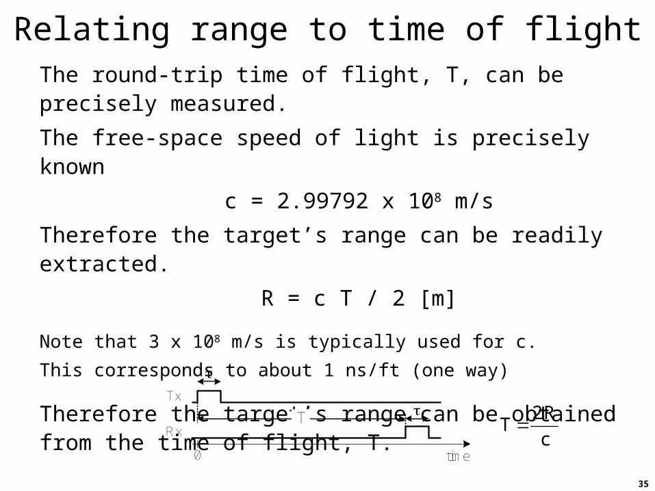
Relating range to time of flightThe round-trip time of flight, T, can be precisely measured.
The free-space speed of light is precisely known
c = 2.99792 x 10⁸ m/s
Therefore the target’s range can be readily extracted.
R = c T / 2 [m]
Note that 3 x 10⁸ m/s is typically used for c.
This corresponds to about 1 ns/ft (one way)
Therefore the target’s range can be obtained from the time of flight, T.
T.
time
Tx
Rx
0c
R2T
36
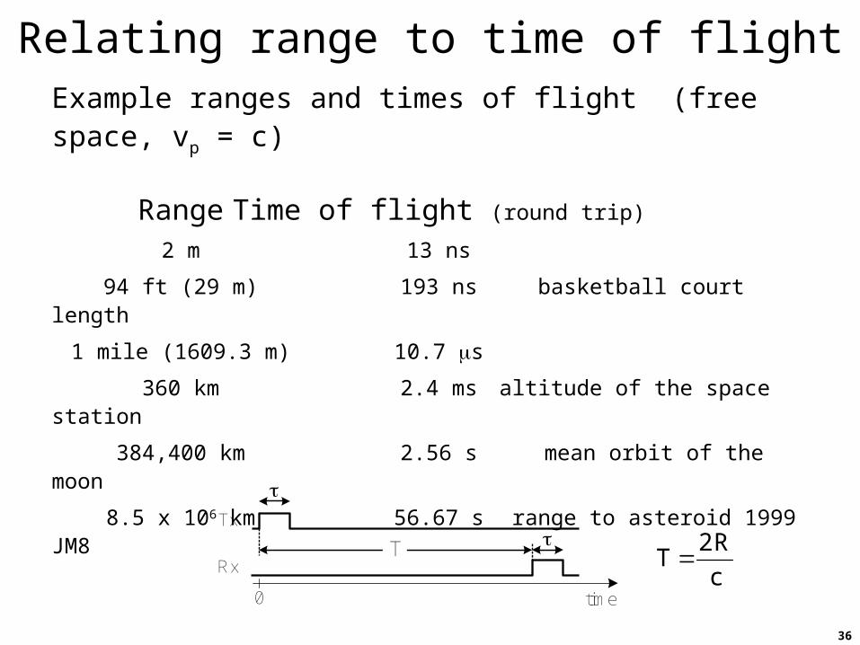
Relating range to time of flightExample ranges and times of flight (free space, vp = c)
Range Time of flight (round trip)
2 m 13 ns
94 ft (29 m) 193 ns basketball court length
1 mile (1609.3 m) 10.7 s
360 km 2.4 ms altitude of the space station
384,400 km 2.56 s mean orbit of the moon
8.5 x 10⁶ km 56.67 s range to asteroid 1999 JM8
T.
time
Tx
Rx
0c
R2T
37
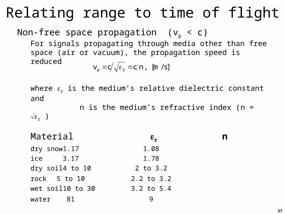
Relating range to time of flightNon-free space propagation (vp < c)
For signals propagating through media other than free space (air or vacuum), the propagation speed is reduced
where r is the medium’s relative dielectric constant and n is the medium’s refractive index (n = r )
Material r ndry snow 1.17 1.08
ice 3.17 1.78
dry soil 4 to 10 2 to 3.2
rock 5 to 10 2.2 to 3.2
wet soil 10 to 30 3.2 to 5.4
water 81 9
]s/m[,nccv rp
38
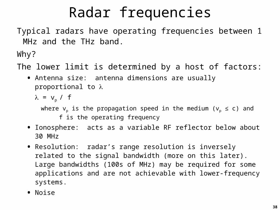
Radar frequenciesTypical radars have operating frequencies between 1 MHz
and the THz band.
Why?
The lower limit is determined by a host of factors:
• Antenna size: antenna dimensions are usually proportional to
= vp / f
where vp is the propagation speed in the medium (vp ≤ c) and
f is the operating frequency
• Ionosphere: acts as a variable RF reflector below about 30 MHz
• Resolution: radar’s range resolution is inversely related to the signal bandwidth (more on this later). Large bandwidths (100s of MHz) may be required for some applications and are not achievable with lower-frequency systems.
• Noise
39
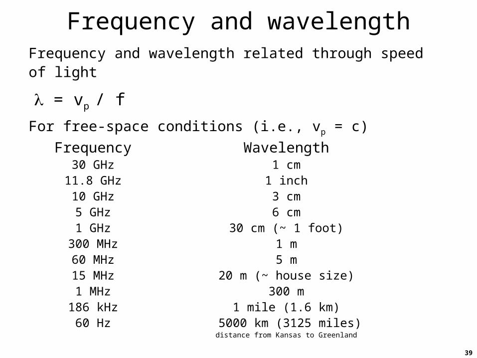
Frequency and wavelengthFrequency and wavelength related through speed of light
= vp / f
For free-space conditions (i.e., vp = c)
Frequency Wavelength30 GHz 1 cm
11.8 GHz 1 inch10 GHz 3 cm5 GHz 6 cm1 GHz 30 cm (~ 1 foot)
300 MHz 1 m60 MHz 5 m15 MHz 20 m (~ house size)1 MHz 300 m
186 kHz 1 mile (1.6 km)60 Hz 5000 km (3125 miles)
distance from Kansas to Greenland
40
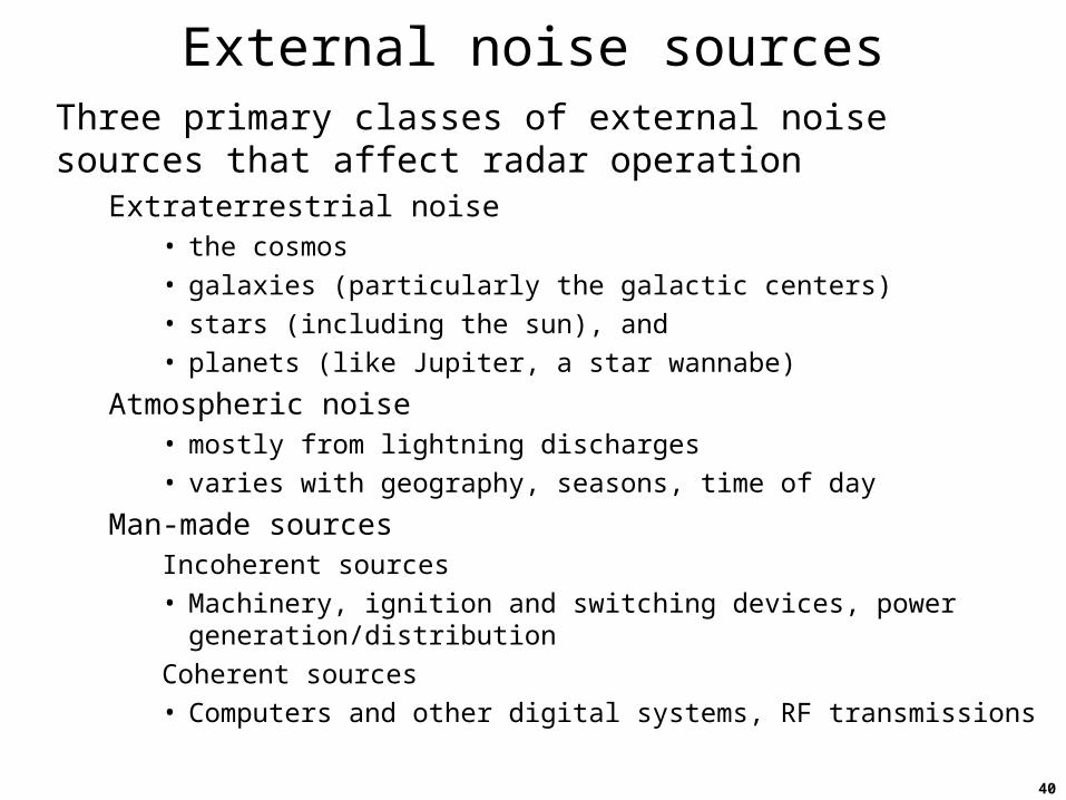
External noise sourcesThree primary classes of external noise sources that affect radar operation
Extraterrestrial noise• the cosmos
• galaxies (particularly the galactic centers)
• stars (including the sun), and
• planets (like Jupiter, a star wannabe)
Atmospheric noise• mostly from lightning discharges
• varies with geography, seasons, time of day
Man-made sourcesIncoherent sources
• Machinery, ignition and switching devices, power generation/distribution
Coherent sources
• Computers and other digital systems, RF transmissions
41
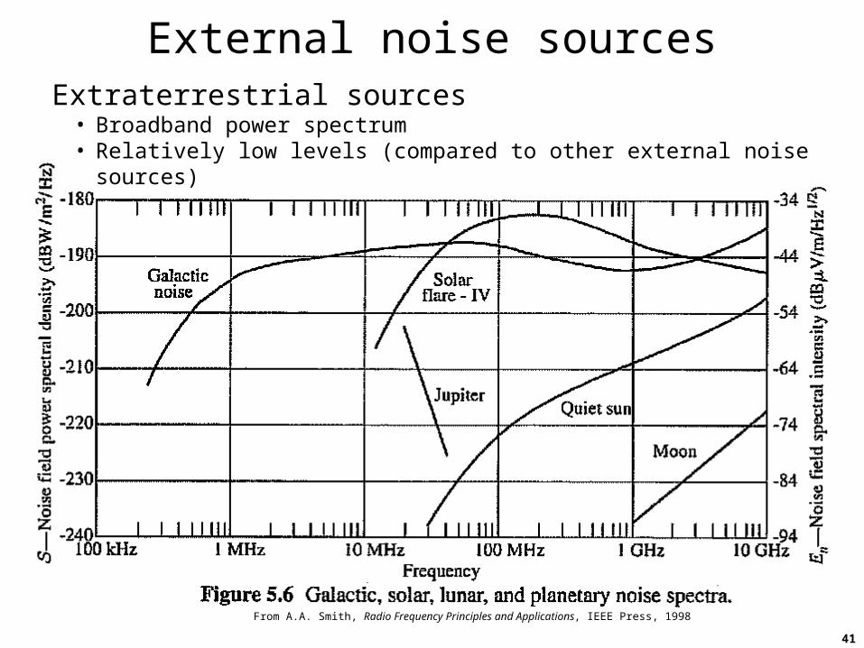
External noise sourcesExtraterrestrial sources
• Broadband power spectrum• Relatively low levels (compared to other external noise sources)
From A.A. Smith, Radio Frequency Principles and Applications, IEEE Press, 1998
42
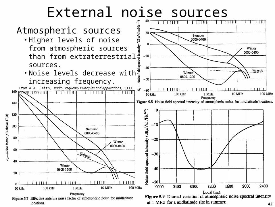
External noise sourcesAtmospheric sources
• Higher levels of noise from atmospheric sources than from extraterrestrial sources.
• Noise levels decrease with increasing frequency.
From A.A. Smith, Radio Frequency Principles and Applications, IEEE Press, 1998
43
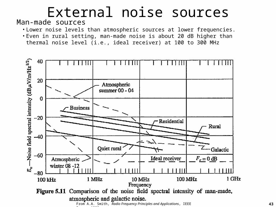
External noise sourcesMan-made sources
• Lower noise levels than atmospheric sources at lower frequencies.• Even in rural setting, man-made noise is about 20 dB higher than
thermal noise level (i.e., ideal receiver) at 100 to 300 MHz
From A.A. Smith, Radio Frequency Principles and Applications, IEEE Press, 1998
44
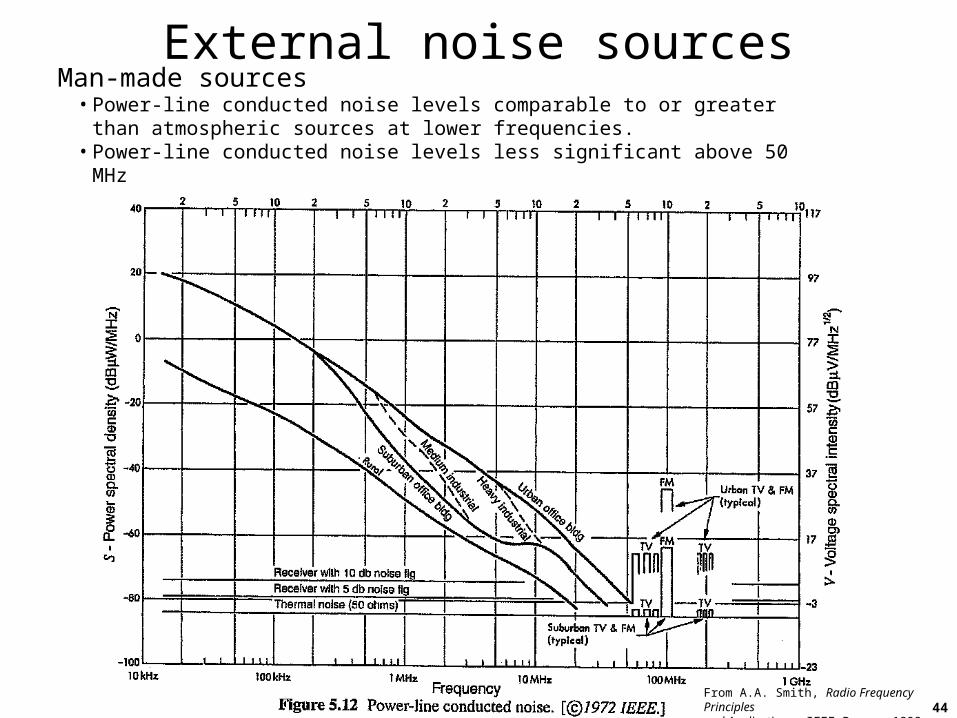
External noise sourcesMan-made sources
• Power-line conducted noise levels comparable to or greater than atmospheric sources at lower frequencies.
• Power-line conducted noise levels less significant above 50 MHz
From A.A. Smith, Radio Frequency Principles
and Applications, IEEE Press, 1998
45
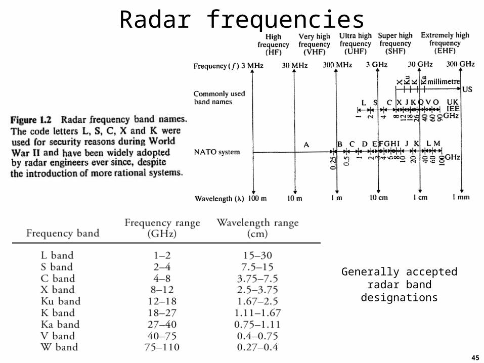
Radar frequencies
Generally accepted radar band designations
46
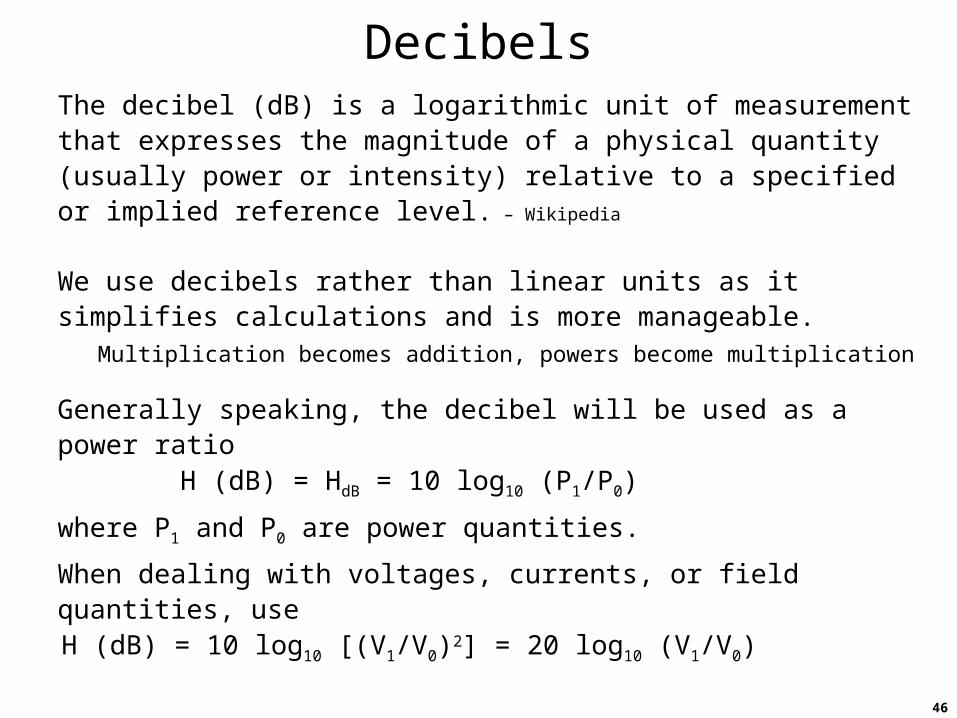
DecibelsThe decibel (dB) is a logarithmic unit of measurement that expresses the magnitude of a physical quantity (usually power or intensity) relative to a specified or implied reference level. – Wikipedia
We use decibels rather than linear units as it simplifies calculations and is more manageable.
Multiplication becomes addition, powers become multiplication
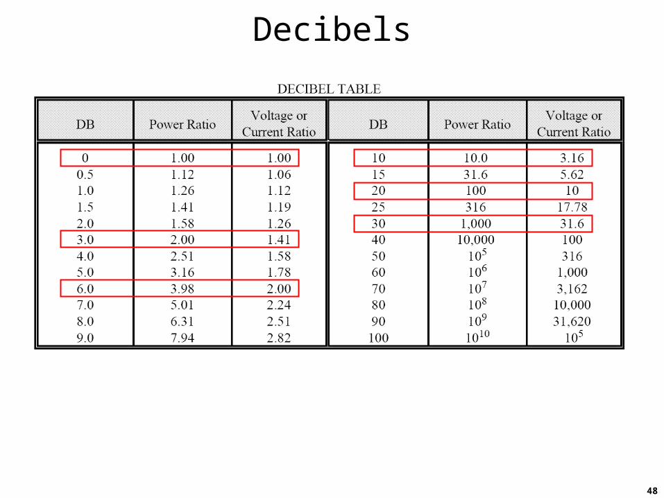
Generally speaking, the decibel will be used as a power ratioH (dB) = HdB = 10 log10 (P1/P0)
where P1 and P0 are power quantities.
When dealing with voltages, currents, or field quantities, useH (dB) = 10 log10 [(V1/V0)2] = 20 log10 (V1/V0)
47
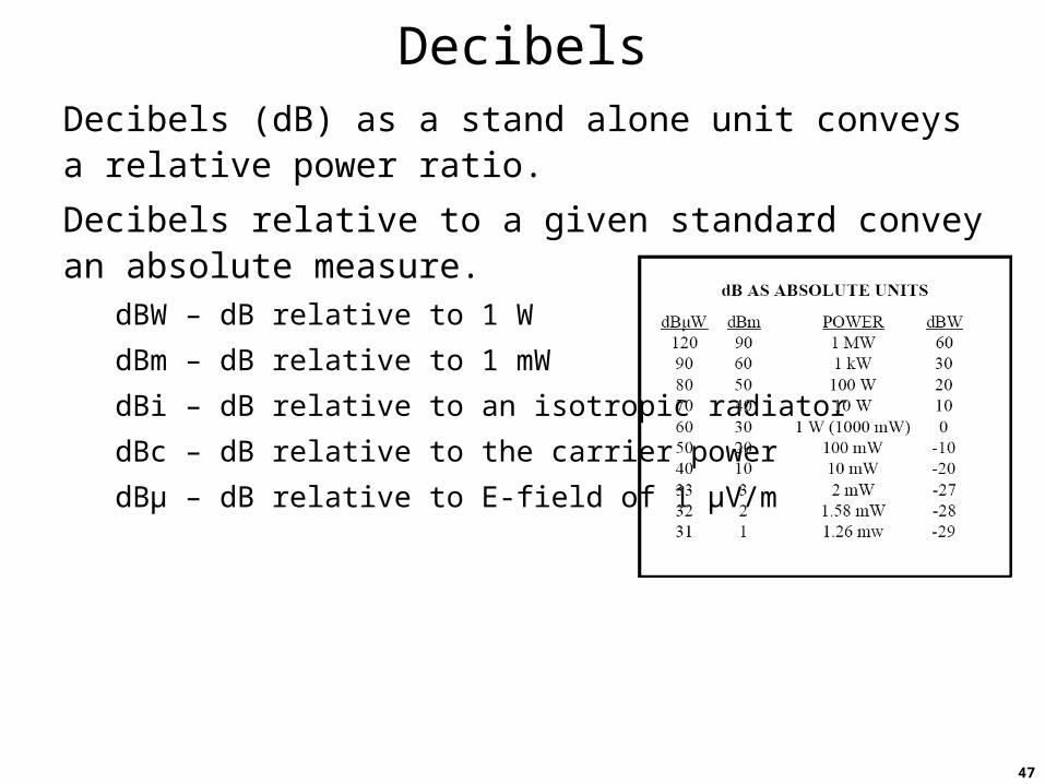
DecibelsDecibels (dB) as a stand alone unit conveys a relative power ratio.
Decibels relative to a given standard convey an absolute measure.
dBW – dB relative to 1 W
dBm – dB relative to 1 mW
dBi – dB relative to an isotropic radiator
dBc – dB relative to the carrier power
dBμ – dB relative to E-field of 1 μV/m
48
Decibels
49
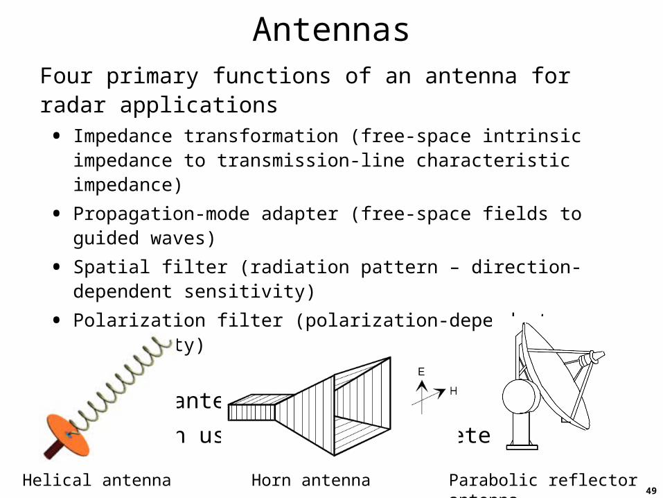
AntennasFour primary functions of an antenna for radar applications
• Impedance transformation (free-space intrinsic impedance to transmission-line characteristic impedance)
• Propagation-mode adapter (free-space fields to guided waves)
• Spatial filter (radiation pattern – direction-dependent sensitivity)
• Polarization filter (polarization-dependent sensitivity)
Important antenna concepts
Computation using antenna parameters
Horn antenna Parabolic reflector antennaHelical antenna
50
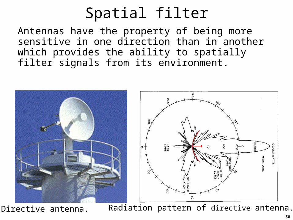
Spatial filterAntennas have the property of being more sensitive in one direction than in another which provides the ability to spatially filter signals from its environment.
Directive antenna. Radiation pattern of directive antenna.
51
Polarization filter
Dipole antenna
Incident E-field vector
z
xy
0EzE V = h E0
+_
EhV
hzh
Incident E-field vector
0EyE
z
xy
V = 0+_
Dipole antenna
EhV
hzh
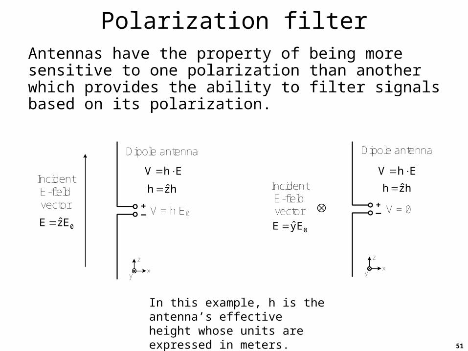
Antennas have the property of being more sensitive to one polarization than another which provides the ability to filter signals based on its polarization.
In this example, h is the antenna’s effective height whose units are expressed in meters.
52
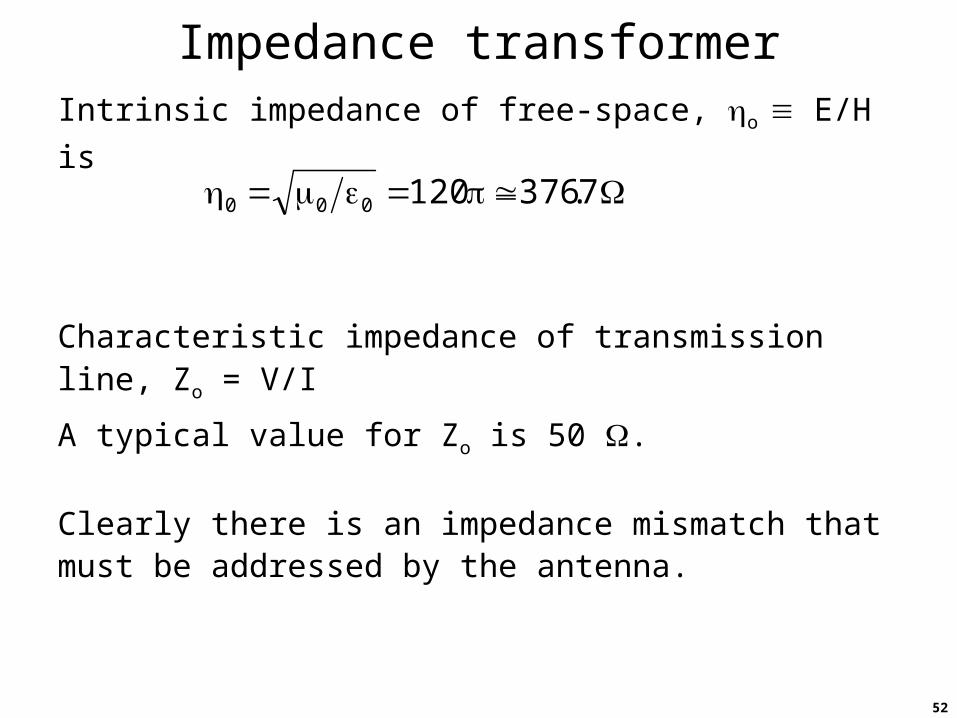
Impedance transformerIntrinsic impedance of free-space, o E/H is
Characteristic impedance of transmission line, Zo = V/I
A typical value for Zo is 50 .
Clearly there is an impedance mismatch that must be addressed by the antenna.
7.376120000
53
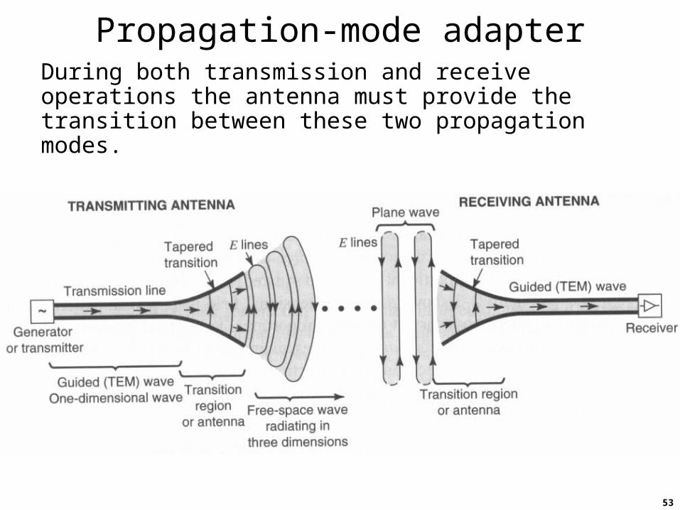
Propagation-mode adapterDuring both transmission and receive operations the antenna must provide the transition between these two propagation modes.
54
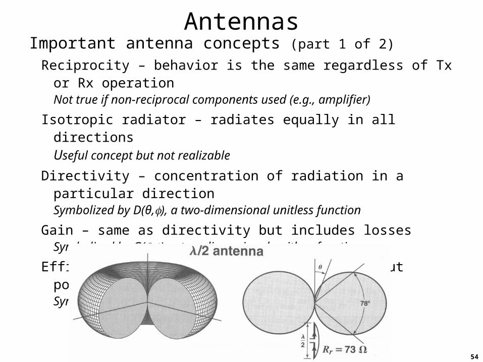
AntennasImportant antenna concepts (part 1 of 2)
Reciprocity – behavior is the same regardless of Tx or Rx operationNot true if non-reciprocal components used (e.g., amplifier)
Isotropic radiator – radiates equally in all directionsUseful concept but not realizable
Directivity – concentration of radiation in a particular directionSymbolized by D(θ,), a two-dimensional unitless function
Gain – same as directivity but includes lossesSymbolized by G(,), a two-dimensional unitless function
Efficiency – ratio of radiated power to input power, think ohmic lossesSymbolized by , ≤ 1
55
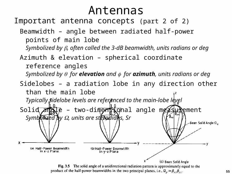
AntennasImportant antenna concepts (part 2 of 2)
Beamwidth – angle between radiated half-power points of main lobeSymbolized by , often called the 3-dB beamwidth, units radians or deg
Azimuth & elevation – spherical coordinate reference anglesSymbolized by for elevation and for azimuth, units radians or deg
Sidelobes – a radiation lobe in any direction other than the main lobeTypically sidelobe levels are referenced to the main-lobe level
Solid angle – two-dimensional angle measurementSymbolized by , units are steradians, Sr
56
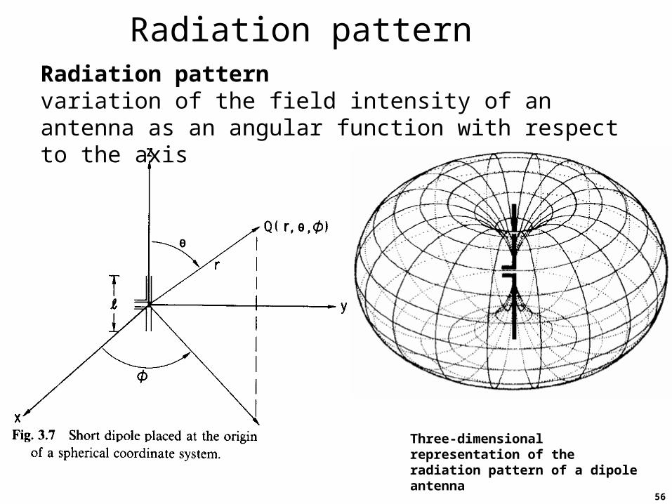
Three-dimensional representation of the radiation pattern of a dipole antenna
Radiation patternRadiation patternvariation of the field intensity of an antenna as an angular function with respect to the axis
57
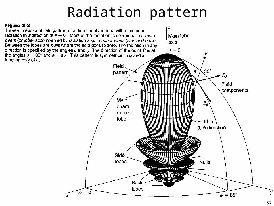
Radiation pattern
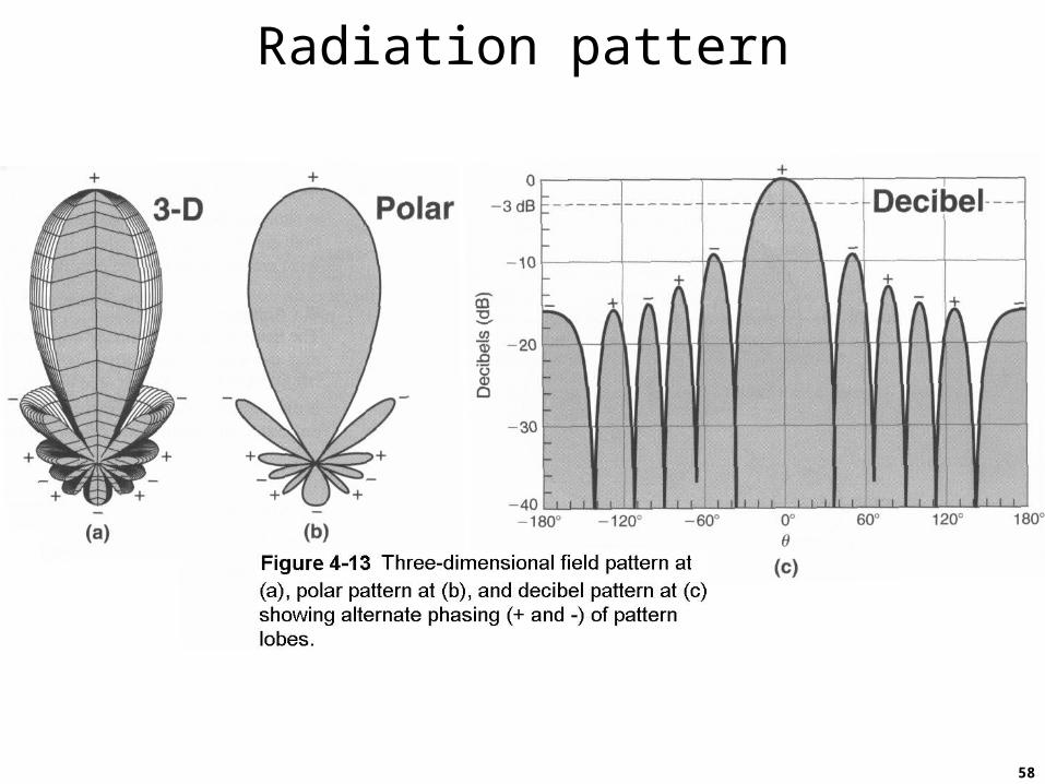
58
Radiation pattern
59
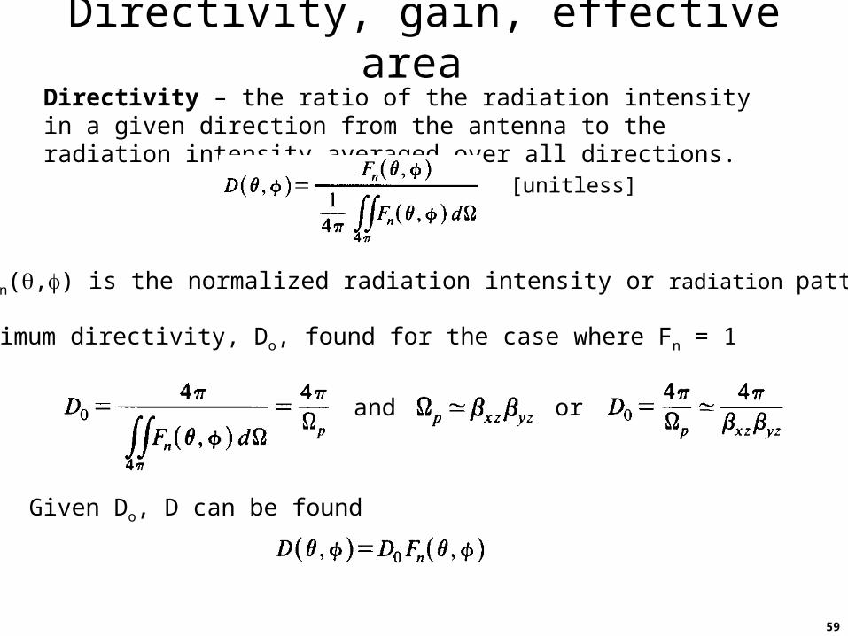
Directivity, gain, effective area Directivity – the ratio of the radiation intensity in a given direction from the antenna to the radiation intensity averaged over all directions.
[unitless]
Maximum directivity, Do, found for the case where Fn = 1
Given Do, D can be found
and or
where Fn(,) is the normalized radiation intensity or radiation pattern [W/Sr]
60
Directivity, gain, effective area
tol PP
olo DG
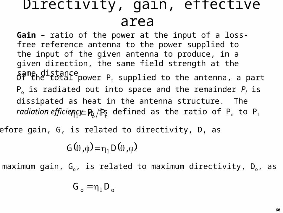
Gain – ratio of the power at the input of a loss-free reference antenna to the power supplied to the input of the given antenna to produce, in a given direction, the same field strength at the same distance
Of the total power Pt supplied to the antenna, a part Po is radiated out
into space and the remainder Pl is dissipated as heat in the antenna
structure. The radiation efficiency l is defined as the ratio of Po to Pt
Therefore gain, G, is related to directivity, D, as
And maximum gain, Go, is related to maximum directivity, Do, as
,D,G l
61
Directivity, gain, effective area
pa2eff20 A4
A4
D
yzxz
2
p
2
effA
yyz l
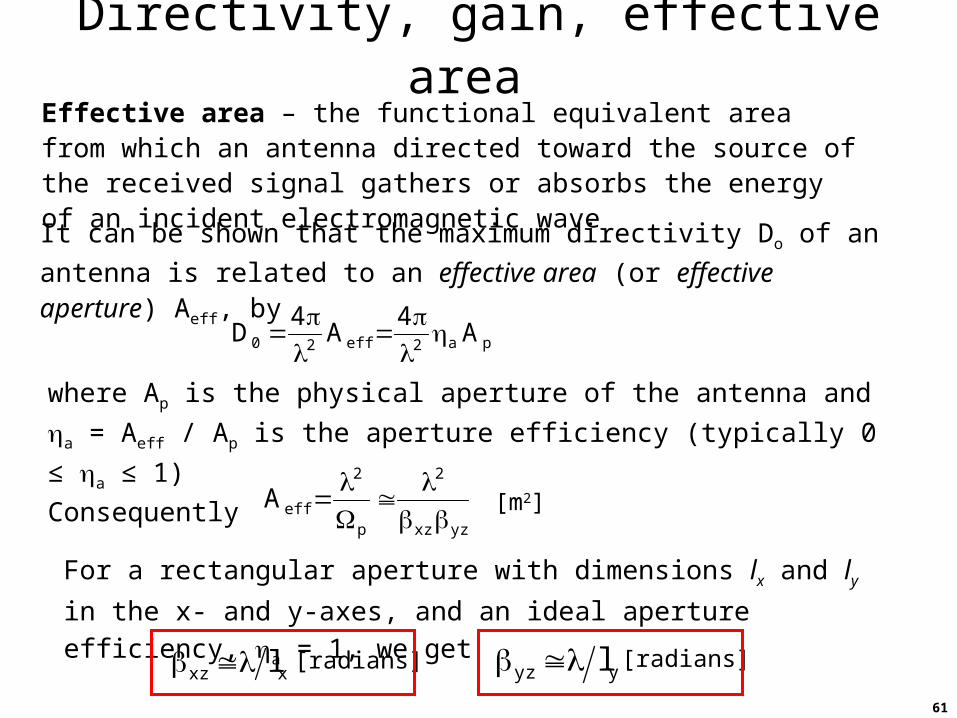
Effective area – the functional equivalent area from which an antenna directed toward the source of the received signal gathers or absorbs the energy of an incident electromagnetic wave
It can be shown that the maximum directivity Do of an antenna is related
to an effective area (or effective aperture) Aeff, by
where Ap is the physical aperture of the antenna and a = Aeff / Ap is the
aperture efficiency (typically 0 ≤ a ≤ 1)
Consequently
For a rectangular aperture with dimensions lx and ly in the x- and y-
axes, and an ideal aperture efficiency, a = 1, we get
xxz l
[m2]
[radians] [radians]
62
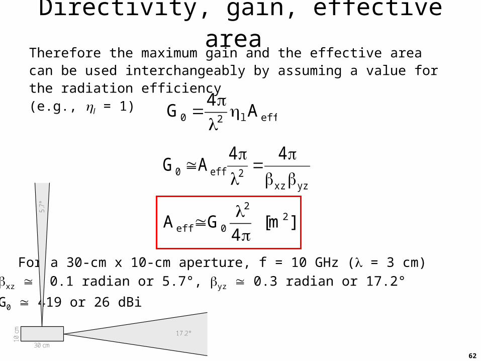
Directivity, gain, effective area Therefore the maximum gain and the effective area can be used interchangeably by assuming a value for the radiation efficiency (e.g., l = 1)
zyzx2eff0
44AG
effl20 A4
G
]m[4
GA 22
0eff
Example: For a 30-cm x 10-cm aperture, f = 10 GHz ( = 3 cm)
xz 0.1 radian or 5.7°, yz 0.3 radian or 17.2°
G0 419 or 26 dBi
17.2°
10 c
m
30 cm
5.7°
63
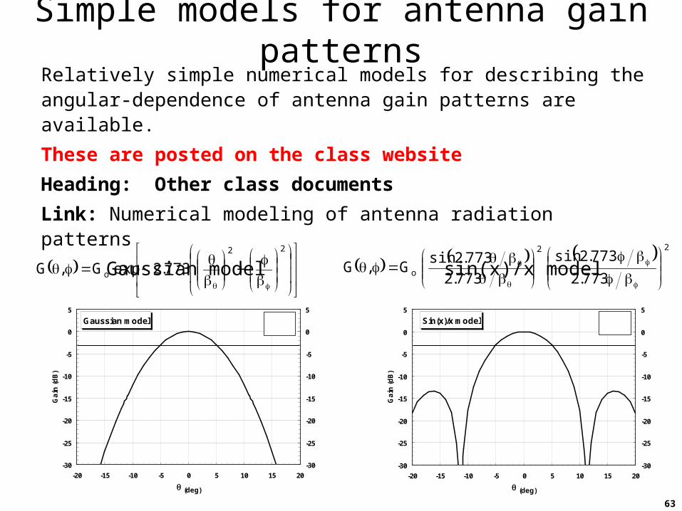
Simple models for antenna gain patternsRelatively simple numerical models for describing the angular-dependence of antenna gain patterns are available.
These are posted on the class website
Heading: Other class documents
Link: Numerical modeling of antenna radiation patterns
Gaussian model sin(x)/x model
22
o 773.2expG,G
Gaussian model
-30
-25
-20
-15
-10
-5
0
5
-20 -15 -10 -5 0 5 10 15 20
(deg)
Ga
in (
dB
)
-30
-25
-20
-15
-10
-5
0
5 = 10o
= 0o
22
o 773.2
773.2sin
773.2
773.2sinG,G
Sin(x)/x model
-30
-25
-20
-15
-10
-5
0
5
-20 -15 -10 -5 0 5 10 15 20
(deg)
Ga
in (
dB
)
-30
-25
-20
-15
-10
-5
0
5 = 10o
= 0o
64
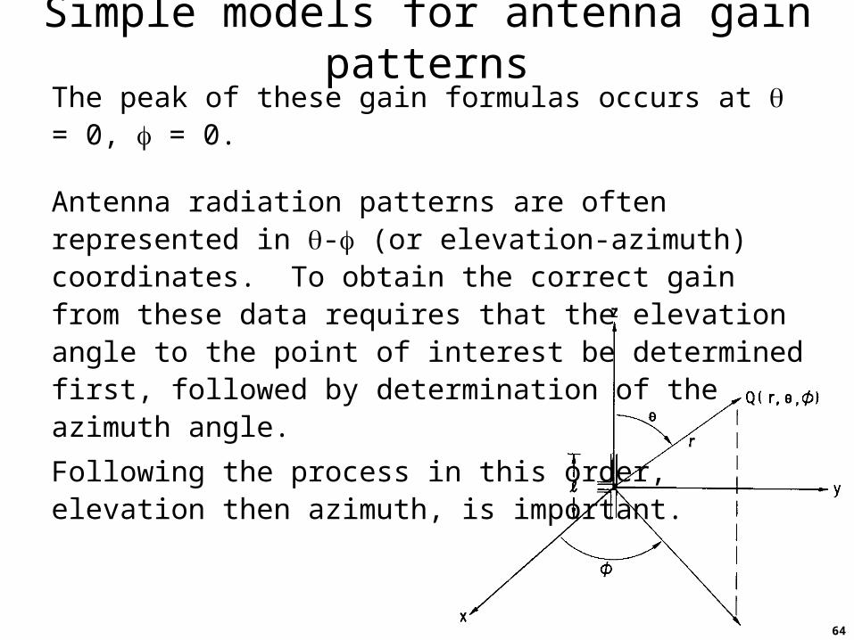
Simple models for antenna gain patternsThe peak of these gain formulas occurs at = 0, = 0.
Antenna radiation patterns are often represented in - (or elevation-azimuth) coordinates. To obtain the correct gain from these data requires that the elevation angle to the point of interest be determined first, followed by determination of the azimuth angle.
Following the process in this order, elevation then azimuth, is important.
65
BandwidthThe antenna’s bandwidth is the range of operating frequencies over which the antenna meets the operational requirements, including:
• Spatial properties (radiation characteristics)
• Polarization properties
• Impedance properties
• Propagation mode properties
Most antenna technologies can support operation over a frequency range that is 5 to 10% of the central frequency
(e.g., 100 MHz bandwidth at 2 GHz)
To achieve wideband operation requires specialized antenna technologies
(e.g., Vivaldi, bowtie, spiral)
66
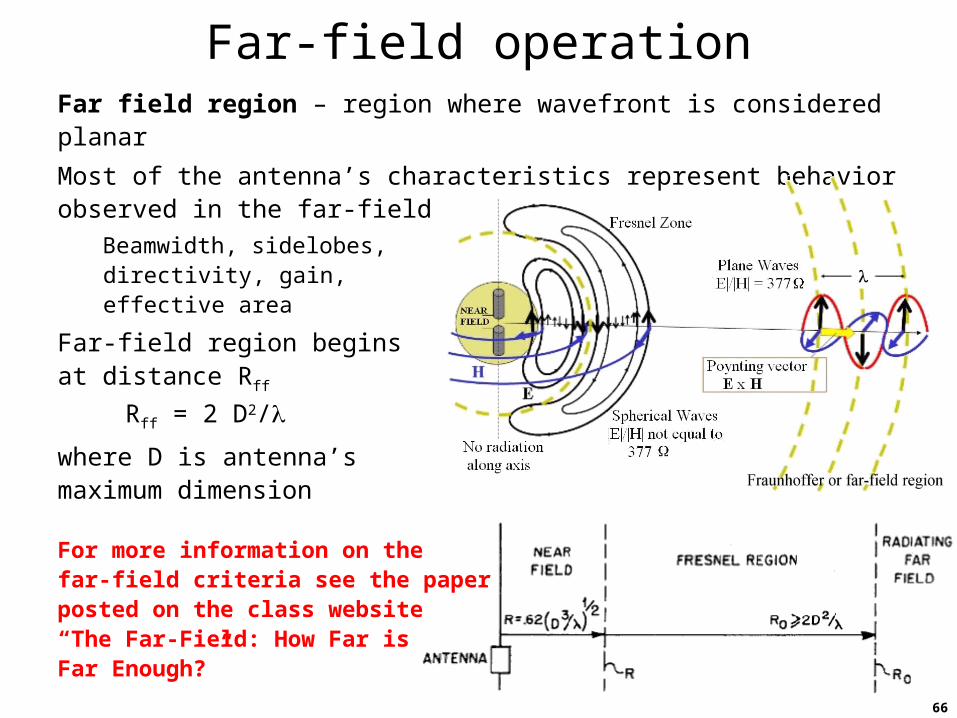
Far-field operationFar field region – region where wavefront is considered planar
Most of the antenna’s characteristics represent behavior observed in the far-field
Beamwidth, sidelobes, directivity, gain, effective area
Far-field region beginsat distance Rff
Rff = 2 D2/
where D is antenna’s maximum dimension
For more information on the far-field criteria see the paper posted on the class website “The Far-Field: How Far is Far Enough?”
67
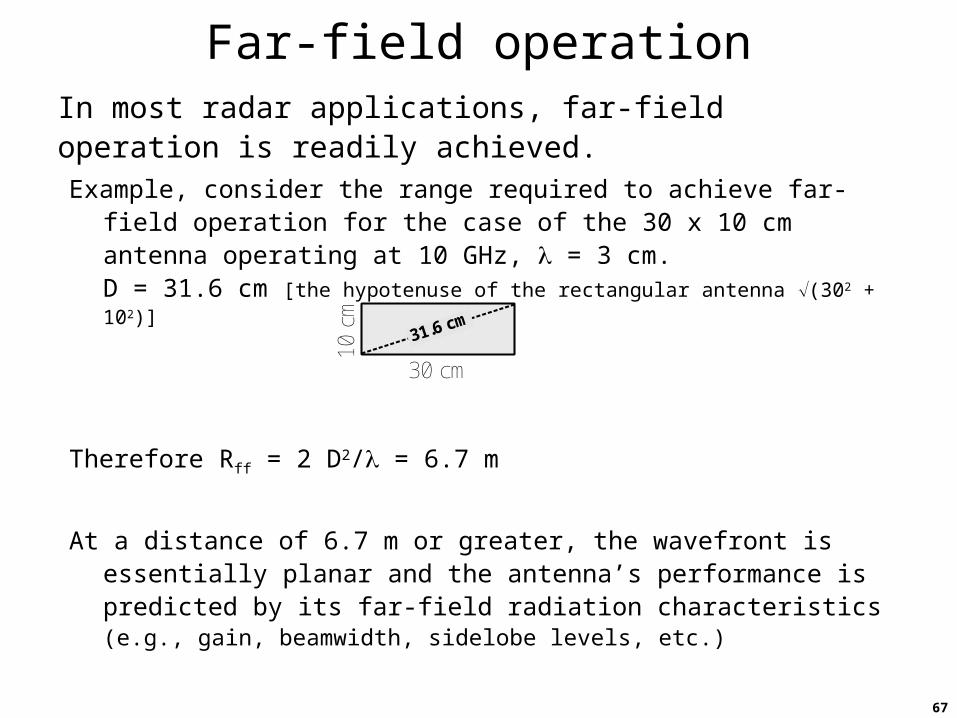
Far-field operationIn most radar applications, far-field operation is readily achieved.Example, consider the range required to achieve far-field operation for
the case of the 30 x 10 cm antenna operating at 10 GHz, = 3 cm.D = 31.6 cm [the hypotenuse of the rectangular antenna (302 + 102)]
Therefore Rff = 2 D2/ = 6.7 m
At a distance of 6.7 m or greater, the wavefront is essentially planar and the antenna’s performance is predicted by its far-field radiation characteristics (e.g., gain, beamwidth, sidelobe levels, etc.)
10 c
m30 cm
31.6 cm
68
Far-field operationThere are cases where far-field operation cannot be assumed.Example, consider laser radar (lidar) with a 1-m operating
wavelength (f = 300 THz) and an antenna (telescope) diameter of 4 (10 cm).In this case Rff = 20 km.
Also, consider the case of a ground-penetrating radar operating at 500 MHz with a 50-cm antenna.The free-space wavelength is c/f = 60 cm.Assume the relative dielectric of the soil to be 6.The wavelength in the soil will be 60 cm / 6 = 24 cm.For this case Rff = 2 m.
However for lossy soil, hardly any significant echoes from 2-m deep targets will be received. Consequently this GPR system will almost always be operating in the antenna’s near field.
69
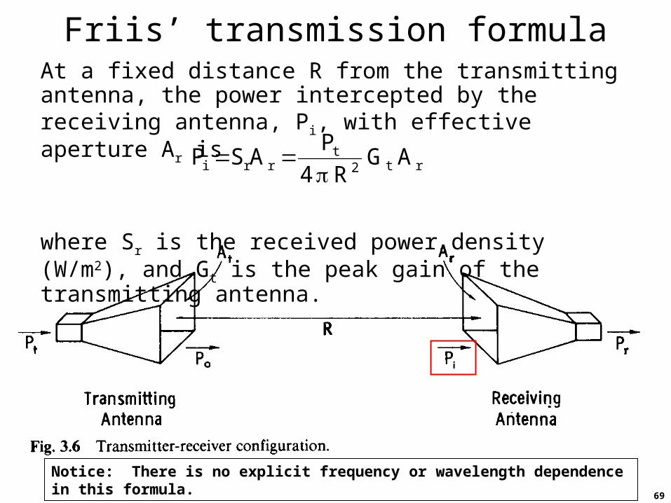
Friis’ transmission formulaAt a fixed distance R from the transmitting antenna, the power intercepted by the receiving antenna, Pi, with effective aperture Ar is
where Sr is the received power density (W/m2), and Gt is the peak gain of the transmitting antenna.
rt2t
rri AGR4
PASP
Notice: There is no explicit frequency or wavelength dependence in this formula.
70
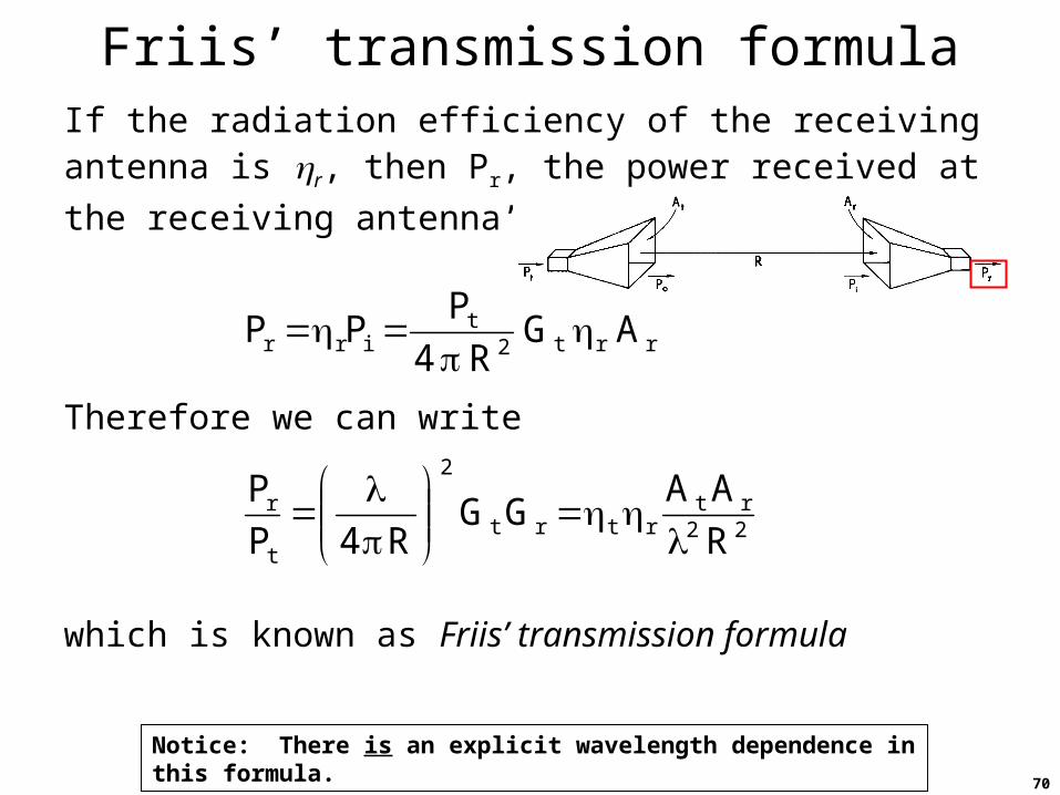
Friis’ transmission formulaIf the radiation efficiency of the receiving antenna is r,
then Pr, the power received at the receiving antenna’s
output terminals, is
Therefore we can write
which is known as Friis’ transmission formula
rrt2t
irr AGR4
PPP
22rt
rtrt
2
t
r
R
AAGG
R4P
P
Notice: There is an explicit wavelength dependence in this formula.
71
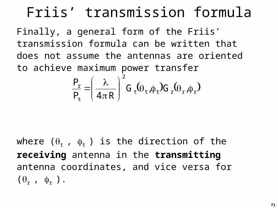
Friis’ transmission formulaFinally, a general form of the Friis’ transmission formula can be written that does not assume the antennas are oriented to achieve maximum power transfer
where (t , t ) is the direction of the receiving antenna in
the transmitting antenna coordinates, and vice versa for (r , r ).
rrrttt
2
t
r ,G,GR4P
P
72
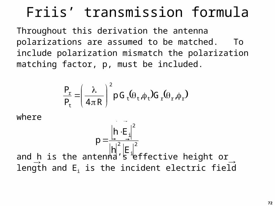
Friis’ transmission formulaThroughout this derivation the antenna polarizations are assumed to be matched. To include polarization mismatch the polarization matching factor, p, must be included.
where
and h is the antenna’s effective height or length and Ei is
the incident electric field
rrrttt
2
t
r ,G,GpR4P
P
2
i
2
2
i
Eh
Ehp
73
Radar range equationTo predict the signal power received by a radar from a target with known radar cross section (RCS) at a given range, the radar range equation (sometimes referred to as simply the radar equation) is used.
The received signal power, Pr, depends on a variety of
system parameters as well as the target’s RCS and range.
Note that the radar equation may be written in a variety of forms for different applications (e.g., point target vs. extended target).
Therefore rather than attempting to memorize the different forms, it may be easier to simply derive the equation, as the derivation is fairly straightforward.
74
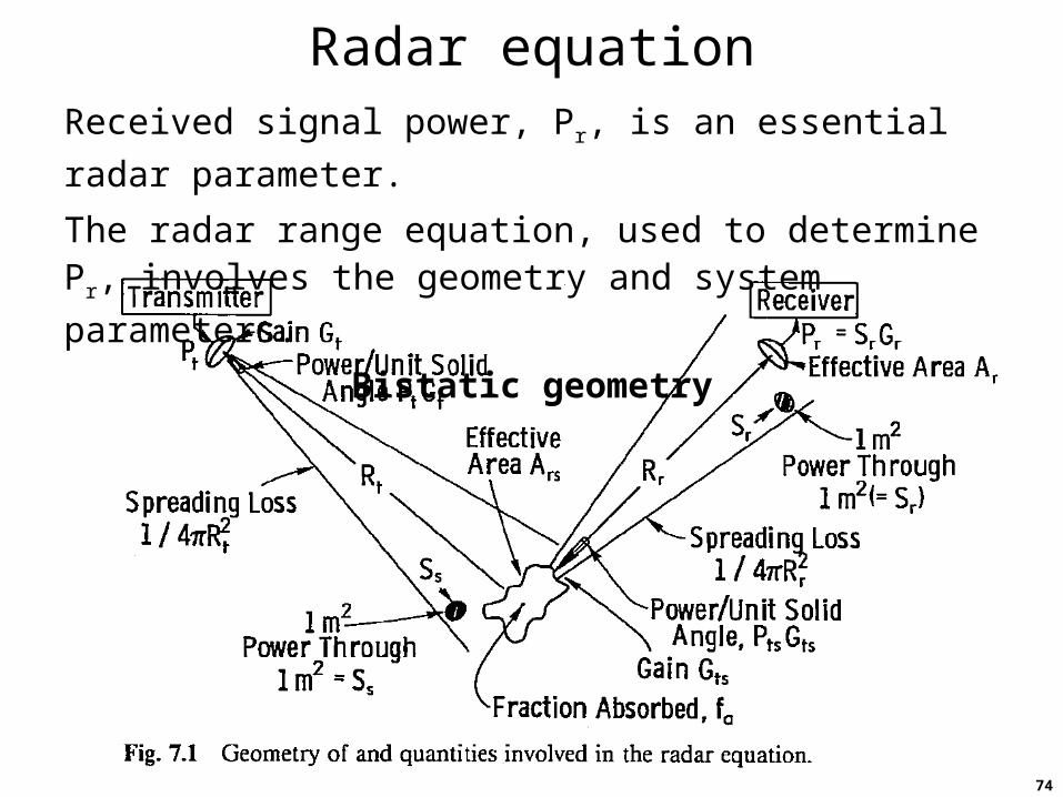
Radar equationReceived signal power, Pr, is an essential radar parameter.
The radar range equation, used to determine Pr, involves
the geometry and system parameters.
Bistatic geometry
75
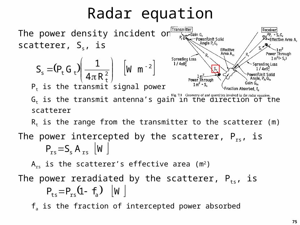
Radar equationThe power density incident on the scatterer, Ss, is
Pt is the transmit signal power (W)
Gt is the transmit antenna’s gain in the direction of the scatterer
Rt is the range from the transmitter to the scatterer (m)
The power intercepted by the scatterer, Prs, is
Ars is the scatterer’s effective area (m2)
The power reradiated by the scatterer, Pts, is
fa is the fraction of intercepted power absorbed
22t
tts mWR4
1GPS
WASP rssrs
Wf1PP arsts
76
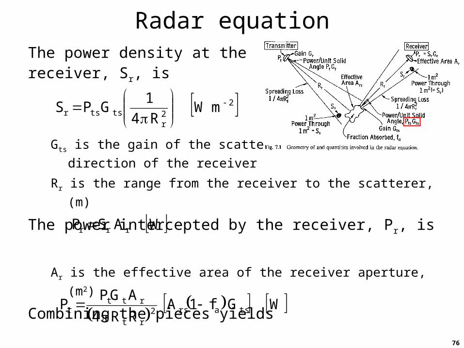
Radar equationThe power density at the receiver, Sr, is
Gts is the gain of the scatterer in the
direction of the receiver
Rr is the range from the receiver to the scatterer, (m)
The power intercepted by the receiver, Pr, is
Ar is the effective area of the receiver aperture, (m2)
Combining the pieces yields
22r
tstsr mWR4
1GPS
WASP rrr
WGf1A
RR4
AGPP tsars2
rt
rttr
77
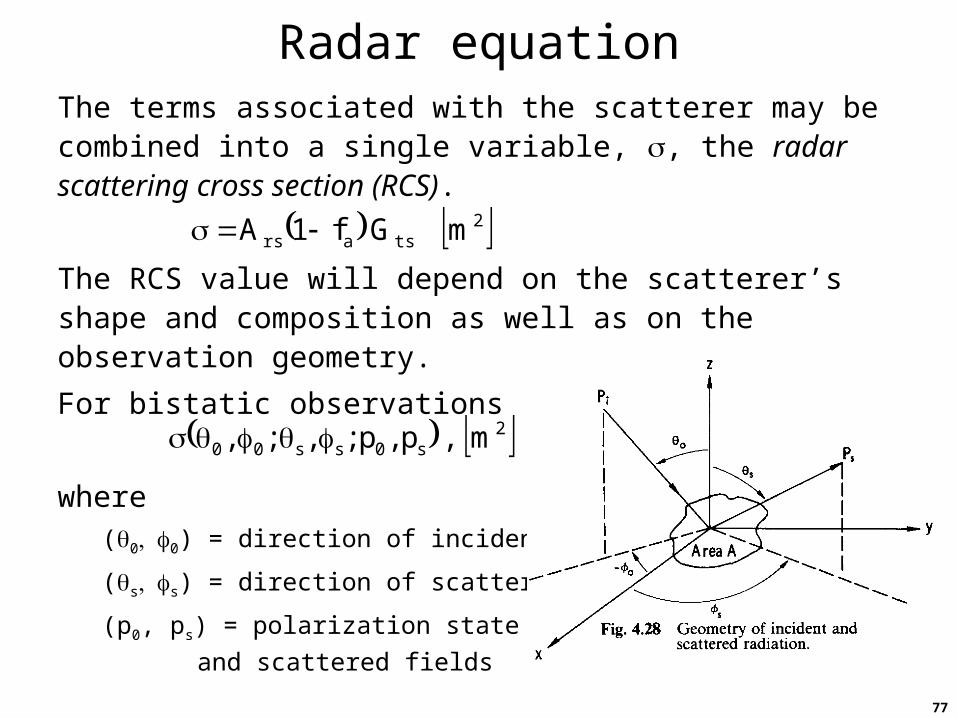
Radar equationThe terms associated with the scatterer may be combined into a single variable, , the radar scattering cross section (RCS).
The RCS value will depend on the scatterer’s shape and composition as well as on the observation geometry.
For bistatic observations
where(00) = direction of incident power
(ss) = direction of scattered power
(p0, ps) = polarization state of incident
and scattered fields
2tsars mGf1A
2s0ss00 m,p,p;,;,
78
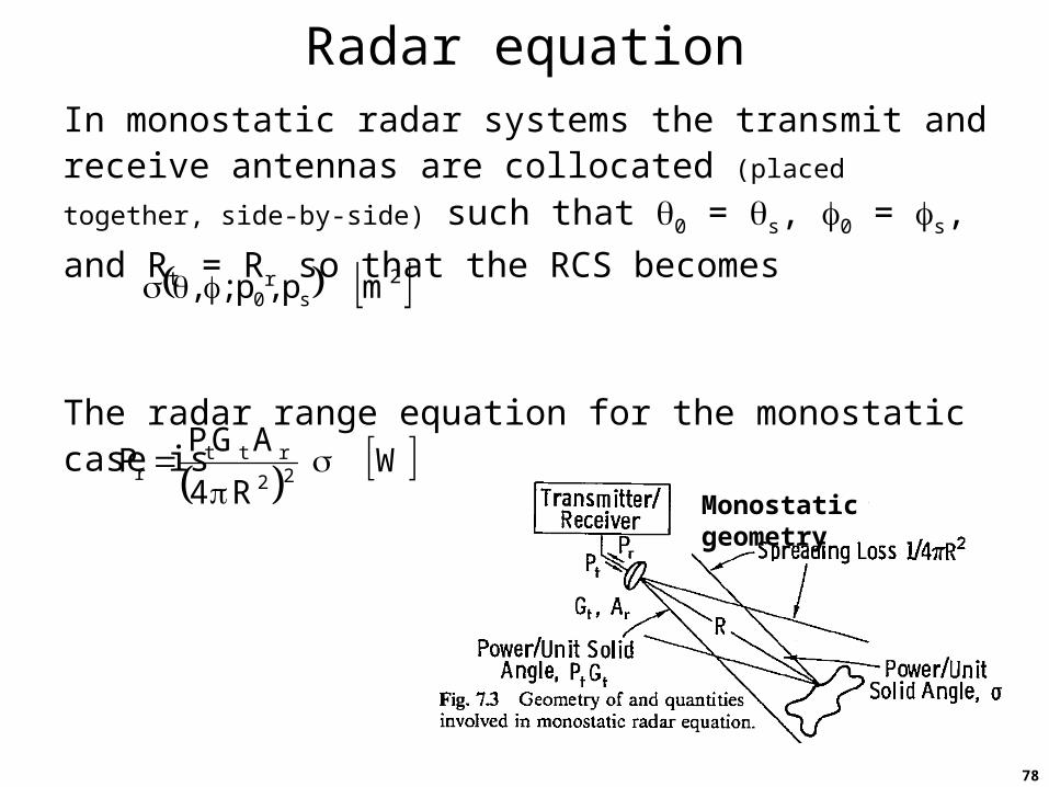
Radar equationIn monostatic radar systems the transmit and receive antennas are collocated (placed together, side-by-side) such that 0 = s, 0 = s, and Rt = Rr so that the RCS becomes
The radar range equation for the monostatic case is
2s0 mp,p;,
WR4
AGPP 22
rttr
Monostatic geometry
79
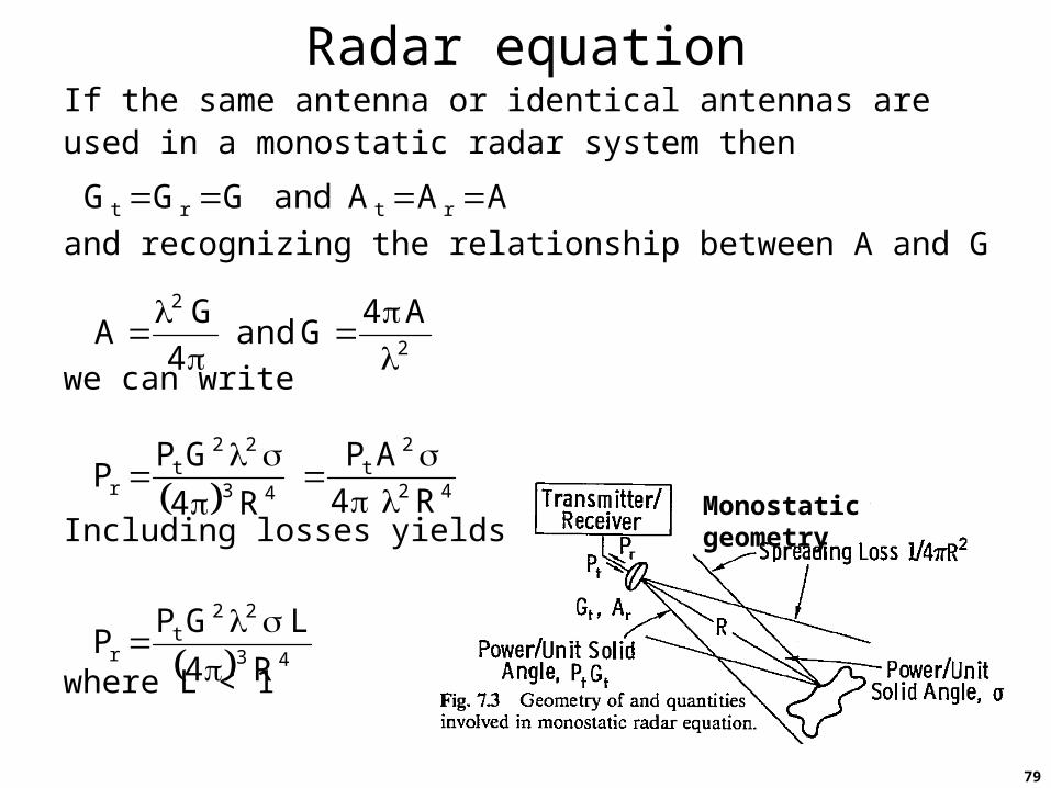
Radar equationIf the same antenna or identical antennas are used in a monostatic radar system then
and recognizing the relationship between A and G
we can write
Including losses yields
where L < 1
AAAandGGG rtrt
2
2 A4Gand
4
GA
42
2t
43
22t
r R4
AP
R4
GPP
Monostatic geometry
43
22t
rR4
LGPP
80
Radar equationExtraction of useful information using signal analysis requires that the signal be discernable from noise, interference, and clutter.
Noise usually originates inside the receiver itself (e.g., receiver noise figure) though may also come from external sources (e.g., thermal emissions, lightning).
Interference is another coherent, spectrally-narrow emission that impedes the reception of the desired signal (e.g., a jammer). [May originate internal or external to radar]
Clutter is unwanted radar echoes that interfere with the observation of signals from targets of interest.
81
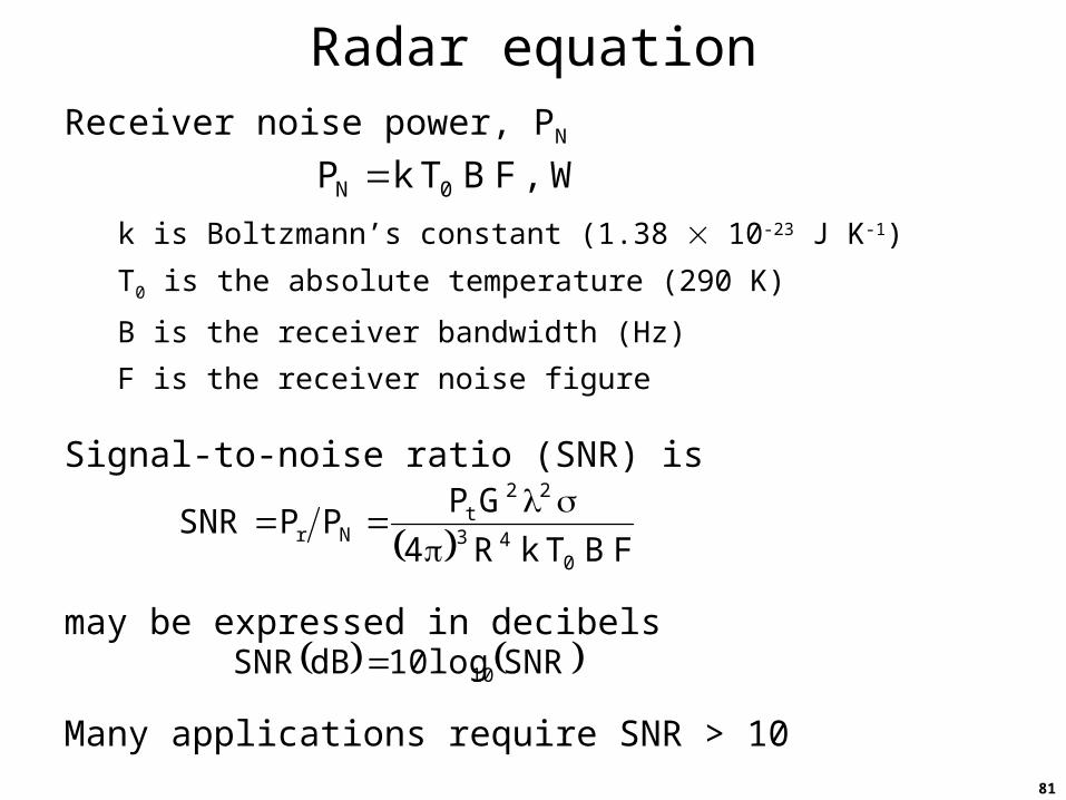
Radar equationReceiver noise power, PN
k is Boltzmann’s constant (1.38 10-23 J K-1)
T0 is the absolute temperature (290 K)
B is the receiver bandwidth (Hz)
F is the receiver noise figure
Signal-to-noise ratio (SNR) is
may be expressed in decibels
Many applications require SNR > 10
W,FBTkP 0N
FBTkR4
GPPPSNR
043
22t
Nr
SNRlog10dBSNR 10
82
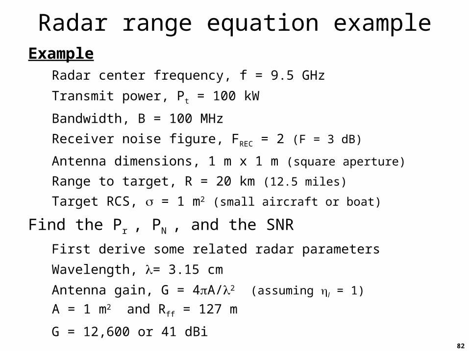
Radar range equation exampleExample
Radar center frequency, f = 9.5 GHz
Transmit power, Pt = 100 kW
Bandwidth, B = 100 MHz
Receiver noise figure, FREC = 2 (F = 3 dB)
Antenna dimensions, 1 m x 1 m (square aperture)
Range to target, R = 20 km (12.5 miles)
Target RCS, = 1 m2 (small aircraft or boat)
Find the Pr , PN , and the SNR
First derive some related radar parameters
Wavelength, = 3.15 cm
Antenna gain, G = 4A/2 (assuming l = 1)
A = 1 m2 and Rff = 127 m
G = 12,600 or 41 dBi
83
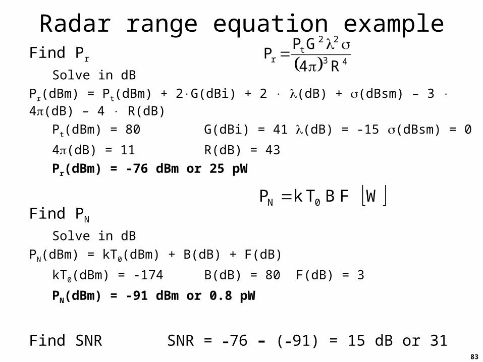
Radar range equation exampleFind Pr
Solve in dB
Pr(dBm) = Pt(dBm) + 2G(dBi) + 2 (dB) + (dBsm) – 3 4(dB) – 4 R(dB)
Pt(dBm) = 80 G(dBi) = 41 (dB) = -15 (dBsm) = 0
4(dB) = 11 R(dB) = 43
Pr(dBm) = -76 dBm or 25 pW
Find PN
Solve in dB
PN(dBm) = kT0(dBm) + B(dB) + F(dB)
kT0(dBm) = -174 B(dB) = 80 F(dB) = 3
PN(dBm) = -91 dBm or 0.8 pW
Find SNR SNR = –76 – (–91) = 15 dB or 31
43
22t
rR4
GPP
WFBTkP 0N
84
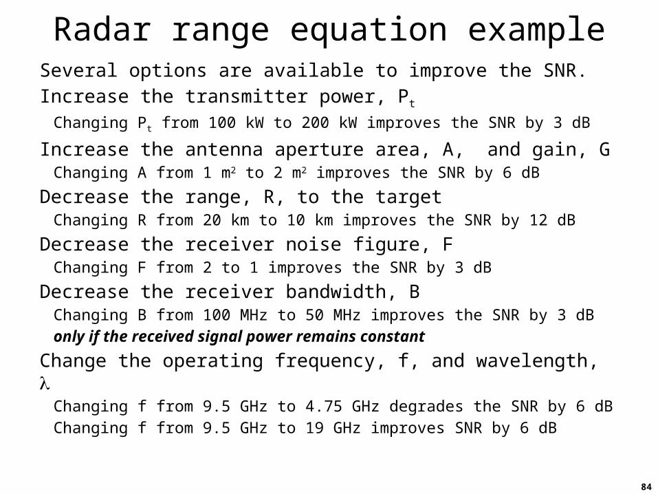
Radar range equation exampleSeveral options are available to improve the SNR.Increase the transmitter power, Pt
Changing Pt from 100 kW to 200 kW improves the SNR by 3 dB
Increase the antenna aperture area, A, and gain, GChanging A from 1 m2 to 2 m2 improves the SNR by 6 dB
Decrease the range, R, to the targetChanging R from 20 km to 10 km improves the SNR by 12 dB
Decrease the receiver noise figure, FChanging F from 2 to 1 improves the SNR by 3 dB
Decrease the receiver bandwidth, BChanging B from 100 MHz to 50 MHz improves the SNR by 3 dB
only if the received signal power remains constant
Change the operating frequency, f, and wavelength, Changing f from 9.5 GHz to 4.75 GHz degrades the SNR by 6 dB
Changing f from 9.5 GHz to 19 GHz improves SNR by 6 dB
85
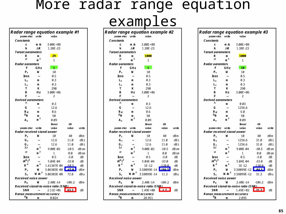
More radar range equation examplesRadar range equation example #1
parameter units value
Constantsc m/s 3.00E+08k J/K 1.38E-23
Target parametersR m 29 m2 1
Radar paramtersf GHz 1Pt W 10
loss -- 0.5Lx m 0.3Ly m 0.3T K 290B Hz 3.00E+06F -- 2
Derived parameters m 0.3G -- 12.6Rff m 0.6DR m 50Ae m2
0.09linear dB
parameter units value value units
Radar received signal powerPt W 10 40 dBmGt -- 12.6 11.0 dBiGr -- 12.6 11.0 dBi2 m2 9.00E-02 -10.5 dBsm m2 1 0.0 dBsm
loss -- 0.5 -3.0 dB(4)-3 -- 5.04E-04 -33.0 dBR-4 m4 1.41387E-06 -58.5 dBPr W 5.06303E-08 -43.0 dBm
Sr W/m25.06303E-08 72.8 dBu
Received noise powerPN W 2.40E-14 -106.2 dBm
Received signal-to-noise ratio (SNR)SNR -- 2.11E+06 63.2 dB
Range measurement accuracydR m 0.024
Radar range equation example #2parameter units value
Constantsc m/s 3.00E+08k J/K 1.38E-23
Target parametersR m 1000 m2 1
Radar paramtersf GHz 1Pt W 10
loss -- 0.5Lx m 0.3Ly m 0.3T K 290B Hz 3.00E+06F -- 2
Derived parameters m 0.3G -- 12.6Rff m 0.6DR m 50Ae m2
0.09linear dB
parameter units value value units
Radar received signal powerPt W 10 40 dBmGt -- 12.6 11.0 dBiGr -- 12.6 11.0 dBi2 m2 9.00E-02 -10.5 dBsm m2 1 0.0 dBsm
loss -- 0.5 -3.0 dB(4)-3 -- 5.04E-04 -33.0 dBR-4 m4 1E-12 -120.0 dBPr W 3.58099E-14 -104.5 dBm
Sr W/m23.58099E-14 11.3 dBu
Received noise powerPN W 2.40E-14 -106.2 dBm
Received signal-to-noise ratio (SNR)SNR -- 1.49E+00 1.7 dB
Range measurement accuracydR m 28.951
Radar range equation example #3parameter units value
Constantsc m/s 3.00E+08k J/K 1.38E-23
Target parametersR m 1000 m2 1
Radar paramtersf GHz 10Pt W 10
loss -- 0.5Lx m 0.3Ly m 0.3T K 290B Hz 3.00E+06F -- 2
Derived parameters m 0.03G -- 1256.6Rff m 6.0DR m 50Ae m2
0.09linear dB
parameter units value value units
Radar received signal powerPt W 10 40 dBmGt -- 1256.6 31.0 dBiGr -- 1256.6 31.0 dBi2 m2 9.00E-04 -30.5 dBsm m2 1 0.0 dBsm
loss -- 0.5 -3.0 dB(4)-3 -- 5.04E-04 -33.0 dBR-4 m4 1E-12 -120.0 dBPr W 3.58099E-12 -84.5 dBm
Sr W/m23.58099E-12 31.3 dBu
Received noise powerPN W 2.40E-14 -106.2 dBm
Received signal-to-noise ratio (SNR)SNR -- 1.49E+02 21.7 dB
Range measurement accuracydR m 2.895
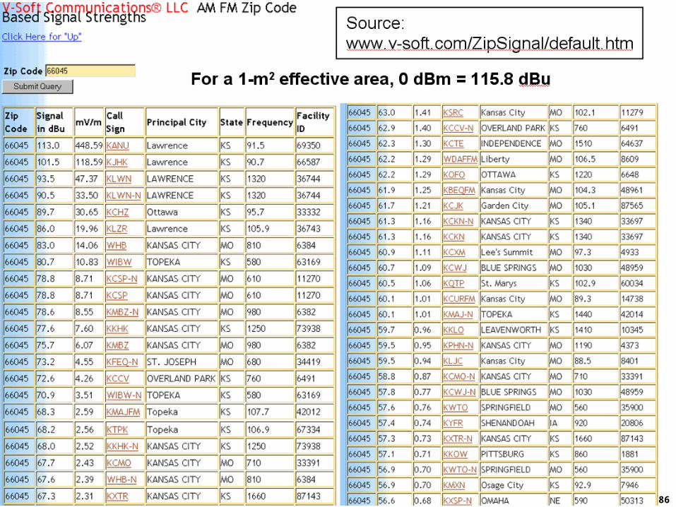
86
87
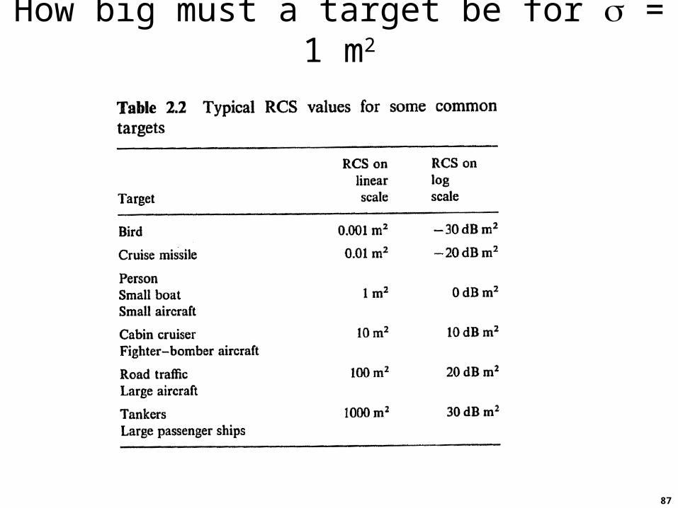
How big must a target be for = 1 m2
88
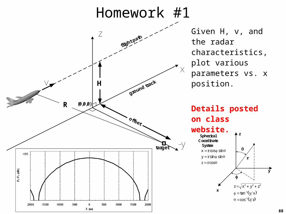
Homework #1Given H, v, and the radar characteristics, plot various parameters vs. x position.
Details posted on class website.
v
x
-y
z
H
flight path
ground track
target
offset
(0,0,0)R
x
y
z
r
Spherical Coordinate
System
cosrz
sinsinry
sincosrx
rzcos
xytan
zyxr
1
1
222
89
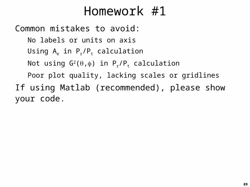
Homework #1Common mistakes to avoid:
No labels or units on axis
Using Ae in Pr/Pt calculation
Not using G2(,) in Pr/Pt calculation
Poor plot quality, lacking scales or gridlines
If using Matlab (recommended), please show your code.