
Bearing capacity failure envelope of suction caissons ... · suction caissons subjected to combined...
133
Bearing capacity failure envelope of suction caissons subjected to combined loading Fortsettelse fra prosjektoppgave Erik Sørlie Civil and Environmental Engineering Supervisor: Gudmund Reidar Eiksund, BAT Co-supervisor: Corneliu Athanasiu, Multiconsult Department of Civil and Transport Engineering Submission date: June 2013 Norwegian University of Science and Technology
Transcript of Bearing capacity failure envelope of suction caissons ... · suction caissons subjected to combined...

Bearing capacity failure envelope of suction caissons subjected to combined loadingFortsettelse fra prosjektoppgave
Erik Sørlie
Civil and Environmental Engineering
Supervisor: Gudmund Reidar Eiksund, BATCo-supervisor: Corneliu Athanasiu, Multiconsult
Department of Civil and Transport Engineering
Submission date: June 2013
Norwegian University of Science and Technology


NORWEGIAN UNIVERSITY OF SCIENCE AND TECHNOLOGY
DEPARTMENT OF CIVIL AND TRANSPORT ENGINEERING
Report Title:
“Bearing capacity failure envelope of suction caissons
subjected to combined loading”
Date: 10/6-2013
Number of pages 130 (I-XIII, 1-117)
Master Thesis x Project Work
Name:
Erik Sørlie
Professor in charge/supervisor:
Gudmund Eiksund and Steinar Nordal
Other external professional contacts/supervisors:
Corneliu Athanasiu
Abstract:
The objective of the master thesis is to use the failure envelope approach to determine the ultimate capacities of a
suction anchor, and to establish a strain-hardening elasto-plastic model in terms of loads and displacements at
padeye.
Numerical analysis in Plaxis 3D has been executed for the suction anchor, which has formed a capacity surface in
terms of combined loading at the padeye. General loading at padeye will result in six force components, which can
be expressed by three independent variables due to constrained loading conditions. Empirical yield surfaces, that
take all six force components into account, have been curve-fitted to the Plaxis results. The yield surfaces have been
used together with load-displacement relations to establish an elasto-plastic formulation with respect to loads and
displacements in terms of the padeye. The results were further generalized, and can be used to estimate the response
of other suction anchors.
The elasto-plasticity has been implemented by isotropic hardening, governed by a curve-fitting hyperbola. The
formulation was implemented in Excel as a spreadsheet that provided accurate results for most load combinations.
The sheadsheet is applicable for both tensile and compression forces, and laod histories for up to 10 steps can be
applied. Each load step in the spreadsheet was divided into 100 load increments. The spreadsheet was made in a
general way, where the input parameters were the ultimate force components, the eccentricities to the neutral planes,
the elastic stiffness coefficients and empirical curve-fitting coefficients with respect to both the yield surface and the
hardening law.
Mesh refinements and hand calculations have been applied. Comparisons show that most load cases have an
adequate convergence; however the torsional capacity was overestimated with about 50%. Analysis without an
activated padeye showed that the overestimation was caused by the flow around mechanism close to the padeye. The
author will recommened to model the anchor without a padeye for later studies, and rather apply a set of force
vectors that give the same load.
Keywords:
1. Offshore Geotechnical Engineering
2. Suction Anchor
3. Combined loading
4. Elasto-plasticity
_________________________________________

I
MASTER DEGREE THESIS
(TBA4900 Geotechnical Engineering, Mater Thesis)
Spring 2013
for
Erik Sørlie
Bearing capacity failure envelope of suction caissons subjected to combined loading
BACKGROUND
There is an increasing focus on use of the failure envelope approach to determine ultimate states of offshore
suction caisson anchors subjected to combined loading (six components of force and moments). The reason
for that is that this approach considers explicitly the independent load components and allows graphical
interpretation of the safety factor associated to different load paths.
The master thesis will use the PLAXIS 3D model of a suction caisson anchor, developed in Project thesis, to
determine the bearing capacity envelope (combination of vertical load, horizontal loads and moments that
cause failure of the supporting soil). The results from PLAXIS 3D analyses will be used to determine the
failure envelope and to express it analytically in non-dimensional form. Numerical experiments will be
undertaken to study the possibility of establishing strain hardening elasto-plastic model in terms of forces
and displacement (force resultant model).
Task description
In developed the Project thesis from 2012, using the PLAXIS 3D results, it was already established a relation
(failure envelope) between horizontal and vertical component of the tension force at failure for a given
geometry of a suction caisson and a given soil profile. It was also found that this relation can be
approximated by a non-dimensional form for all element net refinements (number of elements).
The main goals with the master thesis are:
1. Perform a parameteric study to determine the optimum number of elements that ensures convergence and realistic results
2. Find out whether the suction caisson can be considered rigid (i.e. it only translates and rotates but has no deflections)
3. Find out non-dimensional analytical expression for failure envelope. 4. Study the possibility of establishing an elasto-plastic model in terms of forces and displacements.
This requires establishing whether a yield surface and a hardening parameter can be established. For example if the analytical expression of the failure envelope in terms of vertical and horizontal load components at the pad eye is

II
it might be possible that yield surfaces can be expressed in terms of a hardening parameter
(which can be mobilization degree f = /su) and if
Ho = Hoult*f , Vo = Voult*f, and Mzo = Mzoult*f , then the yield surface has the equation:
In addition, the elastic force-displacement relationship must be defined as:
{ } { } [
] {
} [ ] { }
And a flow rule:
{ } {
}
The formulation of an elasto-plastic model can be used to determine the stiffness of suction caisson
and to construct force-displacement curves along different loading paths.
Professor in charge: Gudmund Eiksund and Steinar Nordal
Other supervisors: Corneliu Athenasiu
Department of Civil and Transport Engineering, NTNU
Date: 06.06.2013
_______________________________________
Professor in charge (signature)

III
Preface
This report is a thesis performed in the spring of 2013 at Geotechnical Division at Norwegian
University of Science and Technology, NTNU. It is an analytical report that contains analyses from
Plaxis 3D, as well as an implementation of an elasto-plastic model.
The duration of the work on the thesis has been 21 weeks, included the Easter. The scope of the
thesis corresponds to 30 credits, which equals one semester of work. The emphasis of the work has
been the following:
- Literature study 20 %
- Modeling and interpretation in Plaxis 3D 30 %
- Establishment of an elasto-plastic model 30 %
- Report writing 20 %
I would like to thank my external supervisor Corneliu Athanasiu and Multiconsult AS for providing an
interesting and challenging exercise and for given me good advices throughout the process.
I would also like to thank my supervisors at NTNU, Gudmund Eiksund and Steinar Nordal. Thanks to
great discussions and good consulting, the work has become more exiting. I will also like to thank the
rest of the geotechnical division and NTNU in general for five great years. The submission of the
thesis implies that an era of my life is over. Thanks to you, I feel that I am ready for the next one.
When I started to work on the thesis, I wanted to produce a comprehensive report that could
actually be used in practice. Weather I have succeeded or not is left to be determined. One thing has
at least become more and more clear to me during the process; do not believe in the answers from a
finite element study if you don’t have many good reasons to do so.
I hope that the reader will find my thesis interesting, and maybe learn something as well. If there is
something that you might wonder about, please do not hesitate to contact me.
Trondheim, 10th of June, 2013
________________________
Erik Sørlie

IV
Summary
The focus of the master thesis is to use the failure envelope approach to determine the ultimate
capacities of a suction anchor, and to establish a strain-hardening elasto-plastic model in terms of
loads and displacements at padeye.
Numerical analysis in Plaxis 3D has been executed for the suction anchor, which has formed a
capacity surface in terms of combined loading at the padeye. The padeye is the connection between
the mooring chain and the anchor, and is located about 2/3 of the anchor length below the seabed.
The suction anchor had an aspect ratio L/D=5, positioned in normally consolidated soft clay, where
undrained conditions with a linear strength profile were assumed. Six force components will be
presented during general loading; three translation forces and three moments. Since the forces will
be applied to the anchor through the padeye, the force components will have constraint relations,
which make it possible to visualize to the response in terms of three independent variables.
Two empirical yield surfaces that accounted for all six force components were curve-fitted to the
obtained capacity surface, and gave appropriate agreement. The average difference between one of
the empirical yield surfaces and the corresponding Plaxis response were 0.70%. The yield surfaces
were further used, together with load deflection relations, to establish an elasto-plastic model in
terms of loads and deflections at padeye position. The formulation was implemented as a
spreadsheet in Excel. The results were then generalized, so that the results can be applied to other
suction anchors.
Mesh refinements and hand calculations were performed in order to ensure that the results from the
numerical study were reasonable. The agreement was adequate to most load cases, however the
torsional resisanse were overestimated with about 50%. The reason is that the flow-around
mechanism that was developed around the padeye, gave an unrealistic resistance. An advice for later
projects would then be to model the padeye either as a rigid link or simply model the padeye forces
as a set of load vectors at the anchor.
The results showed that a misorientation angle of 5 degrees of the padeye with respect to the
mooring chain will decrease the capacity with about 3%, while the capacity will be decreased with
about 12% when the misorientation was 10 degrees. When a larger misorientation degree is present,
the capacity is governed by the ultimate torsional resistance.
The results from the inclined loading showed that the capacity will increase from 0 to 20 degrees,
while the capacity is governed by the ultimate vertical resistance when the inclination angle is 30
degree and more. The results also show that it would be beneficial to lower the padeye position with
2-3 meters.
The failure mechanisms can roughly be divided into three parts. The failure mechanism when the
inclination angle is between 0 and 20 degrees is characterized by rotation about the base of the
anchor. When the inclination angle is 30 degrees or more, the anchor will translate vertically, and a
reversed end bearing mechanism is developed. However, when the torsional angle is 20 degrees or
more, the anchor will rotate about its own axis.

V
The analyses use a linearly- perfectly plastic Mohr-Coulomb material model, and are calculated in
terms of initial reference position.

VI
Contents 1 Introduction ..................................................................................................................................... 1
1.1 Background to the master thesis ............................................................................................ 1
1.2 The purpose of the master thesis ............................................................................................ 1
1.3 The limitations of the master thesis ........................................................................................ 1
1.4 Structure of the report ............................................................................................................ 2
2 Offshore geotechnical engineering ................................................................................................. 3
2.1 Geotechnical engineering ........................................................................................................ 3
2.2 Offshore geotechnical engineering ......................................................................................... 4
2.3 Platform types ......................................................................................................................... 5
2.3.1 Gravity based structures (GBS) ........................................................................................ 6
2.3.2 Jacket platforms .............................................................................................................. 6
2.3.3 Jack-up platforms ............................................................................................................ 7
2.3.4 Compliant towers ............................................................................................................ 7
2.3.5 Tension-leg platforms (TLP) ............................................................................................. 8
2.3.6 FPSs and FPSOs ................................................................................................................ 8
2.4 Applications in offshore geotechnical engineering ................................................................. 8
2.4.1 Piled foundations ............................................................................................................. 8
2.4.2 Shallow foundations ........................................................................................................ 9
2.4.3 Anchors .......................................................................................................................... 10
2.4.4 Gravity anchors ............................................................................................................. 11
2.4.5 Suction anchors ............................................................................................................. 11
2.4.6 Drag anchors .................................................................................................................. 11
2.4.7 Suction embedded plate anchors .................................................................................. 12
2.4.8 Dynamically penetrating anchors .................................................................................. 12
3 Theory ............................................................................................................................................ 13
3.1 Selected theory of soil mechanics ......................................................................................... 13
3.1.1 Stresses .......................................................................................................................... 13
3.1.2 The principle of effective stress .................................................................................... 14
3.1.3 Lateral earth pressure ................................................................................................... 14
3.1.4 Failure criteria and drainage conditions ........................................................................ 15
3.1.5 Bearing capacity ............................................................................................................ 15
3.2 Research on suction anchors ................................................................................................. 17
3.2.1 Installation ..................................................................................................................... 17

VII
3.2.2 Operational conditions .................................................................................................. 18
3.3 Theory of elasto-plasticity ..................................................................................................... 25
3.3.1 Yield criterion ................................................................................................................ 26
3.3.2 Flow rule ........................................................................................................................ 27
3.3.3 Hardening rule ............................................................................................................... 27
3.4 The finite element method ................................................................................................... 28
4 Soil modeling ................................................................................................................................. 30
4.1 Modeling considerations ....................................................................................................... 30
4.2 Soil parameters...................................................................................................................... 30
4.2.1 Strength parameters ..................................................................................................... 30
4.2.2 Stiffness parameters ...................................................................................................... 32
4.2.3 Initial conditions ............................................................................................................ 33
4.3 Properties of the system ....................................................................................................... 33
4.4 Plaxis 3D ................................................................................................................................ 36
4.5 Soil volume ............................................................................................................................ 38
4.6 Failure definition ................................................................................................................... 38
4.7 Mesh refinements ................................................................................................................. 38
5 Results ........................................................................................................................................... 41
5.1 Combined loading.................................................................................................................. 41
5.1.1 Load-deflection curves .................................................................................................. 42
5.1.2 Failure mechanisms ....................................................................................................... 45
5.1.3 Failure surfaces in two dimensions ............................................................................... 48
5.1.4 Three-dimensional plots ................................................................................................ 51
5.2 Hand calculations .................................................................................................................. 52
5.2.1 Horizontal capacity ........................................................................................................ 52
5.2.2 Vertical capacity ............................................................................................................ 53
5.2.3 Bending moment capacity ............................................................................................. 54
5.2.4 Torsional capacity .......................................................................................................... 54
5.2.5 Stiffness ......................................................................................................................... 55
5.2.6 Summary of the hand calculations ................................................................................ 55
5.3 Single-force components with Plaxis 3D ............................................................................... 56
5.4 Stiffness of the anchor .......................................................................................................... 60
5.5 Elastic soil response ............................................................................................................... 61
5.6 Load cycles ............................................................................................................................. 63

VIII
5.7 Curve-fitting yield surfaces .................................................................................................... 65
5.7.1 The first curve-fitting yield surface ............................................................................... 65
5.7.2 The second curve-fitting yield surface .......................................................................... 67
6 Elasto-plastic formulation ............................................................................................................. 75
6.1 Formulation ........................................................................................................................... 75
6.1.1 Compatibility ................................................................................................................. 75
6.1.2 Stiffness and flexibility matrixes .................................................................................... 75
6.1.3 Yield criterion ................................................................................................................ 76
6.1.4 Flow rule ........................................................................................................................ 76
6.1.5 Hardening rule ............................................................................................................... 77
6.1.6 Putting it all together .................................................................................................... 81
6.2 Implementation ..................................................................................................................... 83
6.2.1 Solution steps ................................................................................................................ 83
6.2.2 Elasto-plastic spreadsheet ............................................................................................. 84
6.3 Elasto-plastic response .......................................................................................................... 87
6.3.1 Response against Plaxis results ..................................................................................... 87
6.3.2 Two-way loading ........................................................................................................... 89
6.3.3 Normality ....................................................................................................................... 89
6.4 Elasto-plasticity: Summary .................................................................................................... 90
7 Generalization ............................................................................................................................... 91
7.1 Non-dimensional results ....................................................................................................... 91
7.2 Normalized strength .............................................................................................................. 93
7.3 Non-dimensional stiffness ..................................................................................................... 97
7.4 Elasto-plasticity generalization ............................................................................................ 101
8 Discussion .................................................................................................................................... 102
8.1 Modeling considerations ..................................................................................................... 102
8.2 Reliability of the model ....................................................................................................... 104
8.3 Observations of the capacities ............................................................................................ 106
8.4 Evaluation of the empirical data ......................................................................................... 107
8.5 How to apply the generalized results .................................................................................. 108
9 Conclusion & further work .......................................................................................................... 109
9.1 Conclusion ........................................................................................................................... 109
9.2 Further work ........................................................................................................................ 109
References ........................................................................................................................................... 110

IX
10 Attachments ................................................................................................................................ 112
10.1 Attachment A - Horizontal capacity (Deng & Carter, 2000) ................................................ 113
10.2 Attachment B - Incremental displacements, horizontal planes .......................................... 114
10.3 Attachment C - Flow around mechanism padeye, incremental displacements ................. 115
10.4 Attachment D - Example elasto-plasticity ........................................................................... 116
10.5 Attachment E - Deflection space Plaxis, β=0 ....................................................................... 117

X
Figures
Figure 1 - The first offshore installation, 1947 (Randolph and Gourvenec, 2011) .................................. 4
Figure 2 - Na Kita development, the world's deepest platform, around 2,000 meters (Randolph and
Gourvenec, 2011) .................................................................................................................................... 4
Figure 3 - Gullfaks C - Gravity-based structure, 216 m depth (Randolph and Gourvenic, 2011)............. 4
Figure 4 - catenary, taut and vertical mooring systems .......................................................................... 5
Figure 5 - Overview of anchoring types (Randolph and Gourvenic, 2011) .............................................. 5
Figure 6 - Platform types; (a) Jack-up, (b) GBS, (c) Jacket, (d) Compliant tower, (e) TLP, (f) FPS (Wilson,
2003) ........................................................................................................................................................ 6
Figure 7 - Examples of GBS (Dean, 2009) ................................................................................................ 6
Figure 8 - Typical jacket (Dean, 2009) ..................................................................................................... 7
Figure 9 - Jacket construction; (a) fabrication, (b) transportation, (c) upending, (d) pile construction,
(e) deck and topside installation, (f) pipeline attached (Dean, 2009) ..................................................... 7
Figure 10 - Jack-ups; before and after installation (Dean, 2009) ............................................................ 7
Figure 11 - TLP (Randolph & Gouvenec, 2011) ........................................................................................ 7
Figure 12 - FPS and FPSO (Randolph & Gourvenec, 2011) ...................................................................... 8
Figure 13 - Steel jacket with driven piles - North Rankin A (Randolph, Gourvenec, 2011) ...................... 8
Figure 14 - Flow around mechanism (Randolph & Gourvenec, 2011) ..................................................... 9
Figure 15 - Failure mechanism short pile, horizontal loaded (Randolph & Gourvenec, 2011) ................ 9
Figure 16 - Different applications with shallow foundations. (a)-(b); Gravity-based structures, (c);
Tension-leg platform, (d); Jacket, (e); Subsea frame (Randolph & Gourvenec, 2011) ............................ 9
Figure 17 - Typical jack-up platform with corresponding spudcan foundations (Randolph & Gourvenec,
2011) ...................................................................................................................................................... 10
Figure 18 - Buoyant platforms (Randolph & Gourvenec, 2011) ............................................................ 10
Figure 19 - Gravity box anchor (Randolph & Gourvenec, 2011) ............................................................ 11
Figure 20 - Suction caissons for Laminaria field (Randolph & Gourvenec, 2011) .................................. 11
Figure 21 - Vertically loaded anchor (Randolph & Gourvenec, 2011) ................................................... 11
Figure 22 - Fluke anchor (Randolph & Gourvenec, 2011) ...................................................................... 11
Figure 23 - Suction embedded plate anchor (Randolph & Gourvenec, 2011) ....................................... 12
Figure 24 - Typical dynamically penetrating anchors (Randolph & Gourvenec, 2011) ......................... 12
Figure 25 - Stresses in space (Plaxis, 2010) ........................................................................................... 13
Figure 26 - Stress zones with Mohr-Coulomb (Emdal et al. 2004) ........................................................ 15
Figure 27 - Installation stages with suction anchor (Randolph & Gourvenec, 2011) ............................ 17
Figure 28 - Plug stability (Randolph & Gouvenec, 2011) ....................................................................... 17
Figure 29 - Failure mechanisms: (a) drained, (b) partly drained, (c) undrained conditions (Thorel et al.,
2005) ...................................................................................................................................................... 18
Figure 30 - Current-induced torsion (Lee et al., 2005) ........................................................................... 20
Figure 31 - Failure mechanisms for horizontally loaded suction anchors: (a) translational movement,
(b) rotational movement, (Randolph & Gourvenec, 2011) .................................................................... 21
Figure 32 - Upper and lower bound solution flow-around mechanism (Martin & Randolph, 2006) .... 21
Figure 33 - Horizontal capacity (Randolph et al., 1998) ........................................................................ 22
Figure 34 - Capacity with padeye positions (Supachawarote et al., 2004) ........................................... 22
Figure 35 - HV-load space (El-Sherbiny et al. 2005) .............................................................................. 23
Figure 36 - HV-load space (Taiebat & Carter (2005) ............................................................................. 23

XI
Figure 37 - Normalized HVT-space (Taiebat & Carter (2005) ................................................................ 24
Figure 38 - Vertical loaded pile, Poisson’s ratio of 0.5 (Poulos & David, 1974) ..................................... 24
Figure 39 - Lateral fixed loaded pile (Poulos & David, 1974) ................................................................ 25
Figure 40 - Elasto-plastic response: (a) material without initial yielding plateau, (b) elastic-perfectly
plastic response, (c) hardening material (Irgens, 2008) ........................................................................ 26
Figure 41 - Yield criteria in ∏-plane; von Mises, general yield criterion and Tresca (Irgens, 2008) ...... 27
Figure 42 - Kinematic and isotropic hardening (Irgens, 2008) .............................................................. 27
Figure 43 - Shear strength profile .......................................................................................................... 31
Figure 44 - Thixotropy strength ratio (Jostad & Andersen, 2002) ......................................................... 31
Figure 45 - Linearly elastic-perfectly plastic material model (Plaxis, 2010) .......................................... 33
Figure 46 - Geometry suction anchor. Dimensions in meters when not specified ................................. 34
Figure 47 - Relation between the translational forces .......................................................................... 35
Figure 48 – Elastic and plastic planes and eccentricities ....................................................................... 36
Figure 49 - Soil elements with Plaxis 3D (Plaxis, 2010) ......................................................................... 36
Figure 50 - Area elements with Plaxis 3D (Plaxis, 2010) ....................................................................... 36
Figure 51 - Illustration of interface elements with Plaxis 3D (Plaxis, 2010) .......................................... 37
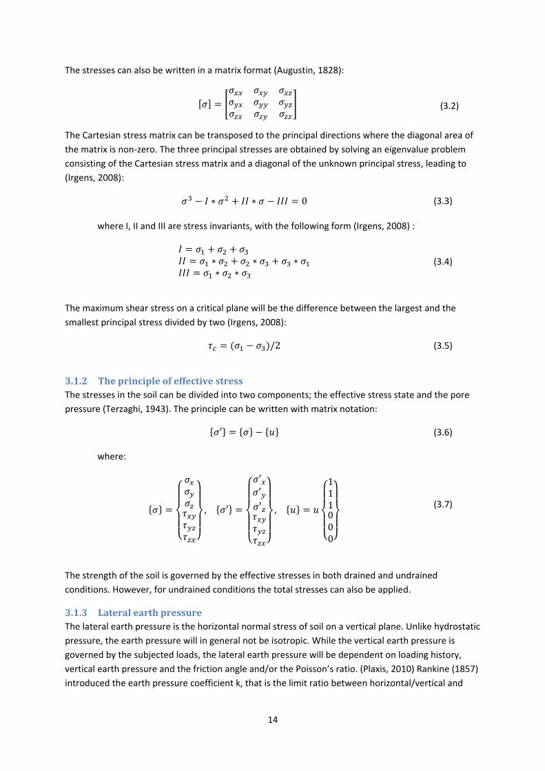
Figure 52 - Mesh refinements; (a) 4,900 el. (b) 11,900 el. (c) 20,500 el. (d) 53,700 el. (e) 182,000 el. . 39
Figure 53 - Convergence - failure load against number of soil elements .............................................. 40
Figure 54 - Locations were a dense mesh is required ............................................................................ 40
Figure 55 - Analyses overview ............................................................................................................... 41
Figure 56 - Load-deflection curve, β=0 degrees .................................................................................... 42
Figure 57 - Load-deflection curve, beta=5 degrees ............................................................................... 43
Figure 58 - Load-deflection, β=10 degrees ............................................................................................ 43
Figure 59 - Load-deflection curve, β=20 degrees .................................................................................. 44
Figure 60 - Load-deflection curve, beta=45 deg .................................................................................... 44
Figure 61 - Load-deflection curve, β=90 degrees .................................................................................. 45
Figure 62 - Incremental strains, β=0 degrees: (a) α=0 degrees, (b) α=20 degrees, (c) α=45 degrees, (d)
α=90 degrees ......................................................................................................................................... 46
Figure 63 - Incremental disp., β=0 degrees: (a) α=0 degrees, (b) α=20 degrees, (c) α=45 degrees, (d)
α=90 degrees ......................................................................................................................................... 47
Figure 64 - Incremental displacements anchor,β=0: (a) α=0, (b) α=10, (c) α=20, (d) α=30, (e) α=45, (f)
α=60, (g) α=90 ....................................................................................................................................... 48
Figure 65 - HV space .............................................................................................................................. 48
Figure 66 - Failure load P with the angles alpha and beta .................................................................... 49
Figure 67 - HV space, failure defined as 5 m deflection ........................................................................ 50
Figure 68 - Yield surface in HV space; deflection criteria: 0.2 m, 0.4 m, 0.6 m, 0.8 m and 1 m ............ 50
Figure 69 - HxHyV space ........................................................................................................................ 51
Figure 70 - P-αβ-space ........................................................................................................................... 51
Figure 71 - Horizontal capacity (Randolph, 1998) ................................................................................. 52
Figure 72 - Factor flow-around mechanism (Martin & Randolph, 2006) .............................................. 52
Figure 73 - Diagrams for the suction anchor ......................................................................................... 53
Figure 74 - Influence factor axially loaded pile (Poulos & David, 1974) ................................................ 55
Figure 75 - Parametric study of ez ......................................................................................................... 57
Figure 76 - Incremental displacements; parametric study of ez ........................................................... 58
Figure 77 - Load-deflection curves......................................................................................................... 59

XII
Figure 78 - Load-displacement curve parametric stiffness .................................................................... 61
Figure 79 - Load deflection; deflections measured in the x-direction ................................................... 62
Figure 80 - Load deflection; deflection measured in the y-direction ..................................................... 62
Figure 81 - Load deflection; deflection measured in the z-direction ..................................................... 63
Figure 82 - Loads and deflections in the x-direction .............................................................................. 64
Figure 83 - Loads and deflections in the y-direction .............................................................................. 64
Figure 84 - Loads and deflections in the z-direction .............................................................................. 64
Figure 85 - Strip load; hand calculated and simplified .......................................................................... 67
Figure 86 - Reduction due to padeye position ....................................................................................... 69
Figure 87 - Yield surfaces, β=0 degrees ................................................................................................. 70
Figure 88 - Yield surfaces, β=5 degrees ................................................................................................. 71
Figure 89 - Yield surfaces, β=10 degrees ............................................................................................... 71
Figure 90 - Yield surfaces, β=20 degrees ............................................................................................... 72
Figure 91 - Yield surfaces, β=45 degrees ............................................................................................... 72
Figure 92 - Yield surfaces, β=90 degrees ............................................................................................... 73
Figure 93 - Plaxis results versus yield surface 2 ..................................................................................... 74
Figure 94 - Empirical curve fitting for hardening; loading in the x-direction ........................................ 78
Figure 95 - Empirical curve fitting for hardening; loading in the y-direction ........................................ 79
Figure 96 - Empirical curve fitting for hardening; loading in the z-direction......................................... 79
Figure 97 - Empirical coefficient values hyperbola ................................................................................ 80
Figure 98 - Hardening curve, α=30 degrees, β=10 degrees; interpolated and optimized based on three
LC, hyperbola ......................................................................................................................................... 80
Figure 99 - Hardening curve, α=30 degrees, β=10 degrees; weighted interpolation and optimized
based on three LC .................................................................................................................................. 81
Figure 100 - Elasto-plastic response; Plaxis and empirical results, β=0 degrees ................................... 87
Figure 101 - Elasto-plastic response; Plaxis and empirical results, β=10 degrees ................................. 88
Figure 102 - Load cycle in the x-direction; Plaxis and empirical isotropic response .............................. 89
Figure 103 - Normality; plastic displacement vectors ........................................................................... 90
Figure 104 - Non-dimensional HV space................................................................................................ 92
Figure 105 - Non-dimensional capacity ................................................................................................. 92
Figure 106 - Vertical capacity factor; wall roughness = 0.4, 0.6, 0.8, Nc=9, W'/(LDsu)=0.54,
su(L)/su=1.89 ......................................................................................................................................... 93
Figure 107 - Normalized results ............................................................................................................. 93
Figure 108 - Normalized HV space with constant mobilized torque ..................................................... 95
Figure 109 - Parametric padeye positions, ez=0-5 meters .................................................................... 96
Figure 110 - Plaxis results compared to hand calculations ................................................................... 96
Figure 111 - The suction anchor; difference between elastic and plastic eccentricities ...................... 100
Figure 112 - Response caused by applied bending moment; (a) failure mechanism, (b) linearly-elastic
response .............................................................................................................................................. 101
Figure 113- Updated and unchanged mesh for vertical load case ...................................................... 102
Figure 114 - Updated and unchanged mesh for the load case pointed in y-direction ........................ 103
Figure 115 - Results from hand calculations and from Plaxis .............................................................. 104
Figure 116 – Respnce with and without the padeye with respect to torsion, inc disp; (a) with padeye
(b) without padeye, (c) response ......................................................................................................... 105
Figure 117 - Comparisons yield surfaces ............................................................................................. 107

XIII
Tables
Table 1 - Mesh refinements .................................................................................................................. 39
Table 2 - Failure loads from padeye loads............................................................................................. 42
Table 3 - Results from hand calculations ............................................................................................... 56
Table 4 - Eccentricities and ultimate forces .......................................................................................... 59
Table 5 - E-modulus load cases ............................................................................................................. 60
Table 6 - Empirical coefficients.............................................................................................................. 66
Table 7 - Empirical coefficients.............................................................................................................. 70
Table 8 - Input parameters .................................................................................................................... 85
Table 9 - Load history ............................................................................................................................ 85
Table 10 - Calculation process for Load Step 1, which is further divided into 100 smaller increments 86
Table 11 - Output data .......................................................................................................................... 86

1
1 Introduction
1.1 Background to the master thesis In recent years, the offshore industry has moved towards deeper waters. Floating platforms have
become more common, and triggered new geotechnical solutions, like the suction anchor that is the
subject of the master thesis. The anchor will be subjected to combined loads from the platform,
caused by environmental loads. The forces are applied to the system through a connection called a
padeye.
The master thesis is an extension of a project work last semester by the same author. The project
focused on the ultimate capacity of a suction anchor subjected to combined loads in undrained
condition. The analysis from that project is replaced with new analyses; the master thesis will for that
reason be an independent work.
1.2 The purpose of the master thesis The purpose of the master thesis is to determine the failure envelope and to establish an elasto-
plastic model of a suction anchor for combined loads by numerical analyses. Six force components
will be presented during general loading; one vertical and two horizontal forces, two bending
moments and a torsional moment. Since the forces will be applied to the anchor through the padeye,
the force components will have constraint relations. The interaction between these constraint forces
will form a yield surface in the loading space. The numerical yield surface will be approximated
empirically by curve fitting. The yield surface, together with load-deflection relations, will be used to
determine the elasto-plastic formulation in terms of padeye loads and deflections. The elasto-plastic
formulation will be at a macro level, and measure the relation between padeye forces and
displacements, rather than the usual relation between stresses and strains.
A suction anchor will always have some degree of misorientation due to the installation. The
misorientation of the padeye with respect to the plane of the mooring chain induces a torsional
moment. One of the aims of the thesis is to determine the impact on the torsional angle due to the
response.
The numerical analysis will be carried out in Plaxis 3D. In order to obtain results with a sufficient
reliability, mesh refinements and hand calculations will be executed. It will also be studied whether
the anchor can be considered rigid, which is important for the soil-structure interaction.
The results from the analysis will also be presented in a non-dimensional matter, so that the work
can be applied to similar situations.
1.3 The limitations of the master thesis The work is limited to one specific suction anchor, with a length-to-depth ratio equal to 5. The
analysis is limited to the undrained condition, where the undrained strength of the soil is almost
proportional to the depth. The soil has been modeled with a linear-perfectly plastic Mohr-Coulomb
material model. The forces are applied to the system through a load vector at the padeye, which is
located almost 2/3 of the length of the anchor from the anchor top. The load vector varies from 0 to
90 degrees with respect to the padeye and the mooring chain and from 0 to 90 degrees between the
horizontal plane and the inclination angle.

2
1.4 Structure of the report The report has the following structure:
Chapter 2 provides an introduction to the topic and offshore geotechnical engineering in general.
Chapter 3 is the theoretical chapter. Basic geotechnical theory, research on suction anchors, elasto-
plastic theory and basics in finite elements will be presented here.
Chapter 4 covers the soil modeling. The soil and structure parameters will be covered, as well as the
model for the report. Plaxis 3D will be discussed briefly and mesh refinements are addressed in this
chapter, since these are essential for convergence.
Chapter 5 covers the results. The results from the different load cases from Plaxis 3D will be
presented, and some failure mechanisms will be shown. The results will be approximated numerically
by curve fitting, and the elastic stiffness of the system will be constructed.
Chapter 6 is devoted to the elasto-plastic formulation. The formulation by means of deflections and
loads applied at padeye, the implementation of the formulation and the results will be presented.
Chapter 7 gives the results in a generalized way, so that the results from the thesis can be used
regarded to other suction anchors. The results will also be presented in a non-dimensional way.
Results from hand calculations will also be included.
Chapter 8 discusses the results and the modeling considerations. The results and their reliability, the
empirical curve fitting and the elasto-plastic formulation will be discussed. In addition, guidelines for
applying the work to other projects will be given.
Chapter 9 concludes the work and outlines proposals for further work.

3
2 Offshore geotechnical engineering This chapter provides an introduction to the subject of suction anchors. Firstly, an overview of
geotechnical engineering will be presented, and then offshore geotechnical engineering will be
introduced. Finally, a summary of applications in offshore geotechnics will be presented.
2.1 Geotechnical engineering Geotechnical engineering deals with the physical properties of the soil. The objective of a
geotechnical calculation is usually to ensure adequate stability of the system and evaluate the
corresponding deformation. Geotechnical engineering is a large field and contains several
applications like:
Slope stability
Settlements calculations
Seepage analysis
Bearing capacity
Earth pressure analysis
The disciplines of geotechnics are applied to all civil engineering problems:
Roads and railways
Natural slopes
Dam engineering
House and building design
Bridge design
Tunneling
Platform design
Port facilities
In all applications, it is essential to obtain information about the physical properties of the site, and
laboratory tests are usually performed prior to design. Unlike when dealing with structural materials,
the uncertainty in material behavior is a large consideration. (Wood, 2009)

4
2.2 Offshore geotechnical engineering Randolph & Gourvenec (2011) provides a comprehensive introduction of the field, and is the
reference most widely used thoughtout this chapter.
Offshore geotechnical engineering is a relatively young discipline, the first fixed installation being
installed in 1947. Today, there are more than 7,000 platforms around the world. Developments in
recent years have moved towards deeper waters. In 1970, the definition of deep water was 50-100
meters, while the definition today is 500 meters and deeper. (Randolph & Gourvenec, 2011)
Figure 1 - The first offshore installation, 1947 (Randolph and Gourvenec, 2011)
Figure 2 - Na Kita development, the world's deepest platform, around 2,000 meters (Randolph and Gourvenec, 2011)
The principles in offshore geotechnics are the same as for traditional geotechnics, although there are
some differences:
Site investigations are more expensive.
Soil conditions are often more difficult
Structural loads are usually significantly larger
The focus is more on capacity rather than deformations, although the stiffness is important
for the dynamical response of the system
Platforms can be divided into two groups: Fixed platforms and
floating platforms. The fixed platform can further be divided into
jackets and gravity-based structures. Jackets usually have a
foundation concept consisting of pile groups in each corner.
Traditionally, gravity-based structures have been directly
embedded is permitted by beneficial soil conditions. However,
when depths became larger, and soil conditions became less
favorable, bucket foundation was adopted.
Figure 3 - Gullfaks C - Gravity-based structure, 216 m depth (Randolph and Gourvenic, 2011)

5
In deeper waters, floating platforms are
preferable. The anchoring keeps the
platform in position. The mooring chain
between the platform and the anchoring
system can be either loose or taut. When
a catenary mooring system is applied, the
cables are resting on the seabed, thus
imposing large horizontal loads on the anchors. For a taut mooring system, the load inclination is
usually more towards the vertical. The load inclination in the mooring system may for that reason
vary from horizontal to vertical, depending on the mooring system. (Randolph & Gourvenec, 2011)
As a consequence of increasingly deeper waters, new anchoring systems have been developed for
floating platforms:
Anchor piles
Suction caisson
Suction embedded plate anchors
Dynamically penetrating anchors
Figure 5 - Overview of anchoring types (Randolph and Gourvenic, 2011)
2.3 Platform types There are numerous platform types, and which platform is best suited for a given project depends on
several factors. Some commonly used platform types will be introduced in the following sections.
Figure 4 - catenary, taut and vertical mooring systems (Randoph & Gourvenec, 2011)

6
Figure 6 - Platform types; (a) Jack-up, (b) GBS, (c) Jacket, (d) Compliant tower, (e) TLP, (f) FPS (Wilson, 2003)
2.3.1 Gravity based structures (GBS)
Gravity based structures are large concrete platforms using their weight to sustain the environmental
loads. The structures are either installed directly at the seabed, or on concrete buckets. GBSs have
been used in waters of up to 300 meters. The topside is supported by one or more concrete legs. In
the case of bucket foundations, installation is achieved by self-weight and suction, when required.
(Dean, 2009)
Figure 7 - Examples of GBS (Dean, 2009)
2.3.2 Jacket platforms
Jackets are the most commonly used platform type for offshore facilities. The jacket consists of an
open framed steel structure, with legs horizontal bracing and diagonal bracing. Jackets are usually
supported by piles, but alternatives like suction anchors have also been applied. In some cases, the
jacket will temporarily be supported by mudmats before pile installation. The piles are then driven,
and a grouted connection between the mudmats and the piles is installed. The deck, the topside and
the pipeline are then installed, and the structure is subsequently ready to sustain the environmental
loads. (Dean, 2009)

7
Figure 8 - Typical jacket (Dean, 2009)
Figure 9 - Jacket construction; (a) fabrication, (b) transportation, (c) upending, (d) pile construction, (e) deck and topside installation, (f) pipeline attached (Dean, 2009)
2.3.3 Jack-up platforms
The jack-up platform is a mobile platform that consists of a topside with holes that are attached to at
least three framed legs. The framed legs are attached to circular shallow foundations called
spudcans, which may have a diameter up to 20 meters. Jack-ups can operate in waters of up to
approximately 150 meters. Firstly, the topside with corresponding legs is floated to the desired
position, where the legs are lowered and penetrated into the seabed. After installation, a proof load
is applied to the system, to ensure that the foundation will have sufficient capacity. (Dean, 2009)
Figure 10 - Jack-ups; before and after installation (Dean, 2009)
2.3.4 Compliant towers
The compliant tower is a platform suited for waters of 300-800 meters,
consisting of a tubular steel truss. The structure is much lighter than a jacket
structure, and is designed to flex with the waves. The structure may be
strengthened by laterally spreading mooring chains supported by anchors. The
truss is usually supported by piles. Due to the flexible response, the crew is
evacuated when storms and hurricanes are expected. (Wilson, 2003) Figure 11 - TLP (Randolph & Gouvenec, 2011)

8
2.3.5 Tension-leg platforms (TLP)
The tension-leg platform is a floating structure, supported by vertically taut cables. The cables are
designed to remain taut for all loadings. The platform has a large mass, which gives a slight response
due to the environmental loads. The platform can be economically competitive in waters of between
300-1200 meters. The cables are usually fixed to foundations anchored by driven piles. In the mid-
1990s, 11 TLPs had been installed; three in the North Sea and eight in the Gulf of Mexico. (Wilson,
2003)
2.3.6 FPSs and FPSOs
In ultra-deep waters, floating production systems (FPS) and floating
production, storage and offloading platforms (FPSO) may be attractive
solutions. The platforms are linked to subsea wells, which are fixed to the
seabed. The floating production platforms will receive and process oil from
subsea wells; often from several fields. The deepest platform currently
installed is a FPS, at about 2,000 meters. Many FPSOs are converted oil
tankers. The FPSO processes and stores the oil from several subsea wells.
Both types of platform are anchored. (Leffler et al. 2011)
2.4 Applications in offshore geotechnical engineering This section will introduce foundation solutions commonly used for offshore platforms. The choice of
solution depends on several factors. Soil conditions are of great importance, and several different
foundation solutions might be appropriate for any given platform type.
2.4.1 Piled foundations
Piled foundation is an attractive solution in
situations where soft soil and high horizontal loads
are present. The piles will then transfer the
structural loads to layers with increased strength.
Piles are especially common for jackets, but might
also be used for anchoring floating facilities like
TLPs. The piles will then be subjected to pull-out
forces. The piles are normally installed by driven
construction regarded to offshore facilities.
(Randolph & Gourvenec, 2011)
Piles in the offshore context usually take a large portion of horizontal loads. However, the interaction
between the vertical and the horizontal loads for slender piles is usually limited, since the horizontal
component is mostly taken by the upper part, while most of the vertical component is taken by the
lower part of the pile. (Randolph & Gourvenec, 2011)
Figure 13 - Steel jacket with driven piles - North Rankin A (Randolph, Gourvenec, 2011)
Figure 12 - FPS and FPSO (Randolph & Gourvenec, 2011)

9
Figure 15 - Failure mechanism short pile, horizontal loaded (Randolph & Gourvenec, 2011)
2.4.2 Shallow foundations
Shallow foundations are advantageous when soil conditions at the seabed are favorable. Shallow
foundations are often applied with jackets, gravity-based structures and jack-ups. Jackets are often
supported by steel mudmats before the installation of piles. Gravity-based structures are either
installed directly on the seabed or on bucket foundations. Jack-ups are usually supported by
spudcans, which are circular plates that are, during installation, pushed until the desired capacity is
achieved. (Randolph & Gourvenec, 2011)
Figure 16 - Different applications with shallow foundations. (a)-(b); Gravity-based structures, (c); Tension-leg platform, (d); Jacket, (e); Subsea frame (Randolph & Gourvenec, 2011)
In the early development of gravity-based structures, soil conditions were beneficial due to heavily
over-consolidated soil, and direct foundations were used. Later on, when the offshore industry
moved towards deeper waters, soil conditions became less favorable and bucket foundations were
required. The buckets are installed by self-weight only, in cases where the weight of the platform is
adequate relative to the surrounding soil. Otherwise, suction will be applied in the final stage of
installation. In case of floating facilities, suction is usually applied during installation. (Randolph &
Gourvenec, 2011)
Figure 14 - Flow around mechanism (Randolph & Gourvenec, 2011)

10
Figure 17 - Typical jack-up platform with corresponding spudcan foundations (Randolph & Gourvenec, 2011)
2.4.3 Anchors
Anchors are required to keep floating facilities in position. Floating facilities are suited for deep
waters, where fixed platforms would not be economical. (Wilson, 2003)
Figure 18 - Buoyant platforms (Randolph & Gourvenec, 2011)
The increasing focus on deep waters has triggered new anchor solutions. The loads from the platform
are transferred to the anchor system by mooring chains that are attached to an amplified
connection. The cables between the platform and the anchors can be either taut or loose. The
appropriate foundation solution depends on the loading and the soil conditions. (Randolph &
Gourvenec, 2011) The most common anchor systems will now be presented separately, although
anchor piles will not be covered, since these have already been presented.

11
2.4.4 Gravity anchors
Gravity anchors can be applied if the required holding
capacity is limited. The capacity is generated from
dead weight and friction between the anchor and the
seabed. A large portion of the dead weight is often due
to filled rocks. (Randolph & Gourvenec, 2011)
2.4.5 Suction anchors
Suction anchors are large steel cylinders, with a
typical length-to-depth ratio of 2-6. Suction
anchors are most commonly used with FPSs and
FPSOs. Suction anchors are installed in two steps;
firstly the anchor penetrates by self-weight, then
suction is applied by pumping water out of the
top. One of the advantages of suction anchors is
the simple installation that accurately puts the
anchor in position. (Randolph & Gourvenec, 2011)
The research on suction anchors will be covered
in chapter 3.2.
2.4.6 Drag anchors
Drag anchors are characterized by their installation, where the anchor is positioned by a drag length.
The anchors are relatively light and have a large capacity-to-weight ratio. The capacity of drag
anchors comes from the soil in front of the anchor. Drag anchors can further be divided into fluke
anchors and vertically loaded anchors. Fluke anchors are applied when the load is mostly horizontal.
Despite their benefits, drag anchors require a more complicated installation, where it might be
challenging to achieve the desired position. The experience with drag anchors on permanent floating
facilities is also limited. (Randolph & Gouvenec, 2011)
Figure 22 - Fluke anchor (Randolph & Gourvenec, 2011)
Figure 19 - Gravity box anchor (Randolph & Gourvenec, 2011)
Figure 20 - Suction caissons for Laminaria field (Randolph & Gourvenec, 2011)
Figure 21 - Vertically loaded anchor (Randolph & Gourvenec, 2011)

12
2.4.7 Suction embedded plate anchors
The suction embedded plate anchor is similar to the suction anchor, although a plate is fitted at the
bottom of the anchor. The anchor combines the benefits of a suction anchor and a plate anchor in
the sense that installation is efficient, and the plate makes the system more economical. Although
the anchor is more optimized than the suction anchor, the installation phase requires more time and
there is limited experience with the anchor (Randolph & Gourvenec, 2011).
Figure 23 - Suction embedded plate anchor (Randolph & Gourvenec, 2011)
2.4.8 Dynamically penetrating anchors
The dynamically penetrating anchors have a missile-
like shape and are well suited for penetration into the
soil. The anchors are released about 20-50 meters
above the seabed and will reach velocities in the range
of 25-35 m/s. The advantages of these anchors are
their simple production and installation. The primary
disadvantage is the lack of experience. (Randolph &
Gourvenec, 2011).
Figure 24 - Typical dynamically penetrating anchors (Randolph & Gourvenec, 2011)

13
3 Theory This theory chapter will provide a framework for the topics discussed in the thesis. Firstly, the most
relevant theory of soil mechanics will be outlined, before mentioning research on suction anchors.
Thereafter, a review of the theory of elasto-plasticity will be given, before introducing the finite
element method.
3.1 Selected theory of soil mechanics Since the scope on this thesis is limited to the ultimate capacity and the stiffness relations, the theory
part will focus on these topics.
3.1.1 Stresses
The stresses in the soil will in general be related to loading history and the strains in the soil. Unlike
structural materials, the relation between stresses and strains will usually not be linear. It is still
common to assume linear elasticity in settlement calculations and to model the elastic range of an
elasto-plastic material as linearly-elastic. The elastic relations between the stresses and the strains
are dependent of the Young’s modules (Young, 1845) and the Poisson’s ratio (Poisson, 1833). The
constitutive relations are the following (Augustin, 1828):
{
}
[
]
{
}
(3.1)
where σ is normal stress
τ is shear stress
E is the Young’s modulus
υ is the Poisson’s ratio
ε is normal strains
γ is shear strains
Figure 25 - Stresses in space (Plaxis, 2010)
14
The stresses can also be written in a matrix format (Augustin, 1828):
[ ] [
] (3.2)
The Cartesian stress matrix can be transposed to the principal directions where the diagonal area of
the matrix is non-zero. The three principal stresses are obtained by solving an eigenvalue problem
consisting of the Cartesian stress matrix and a diagonal of the unknown principal stress, leading to
(Irgens, 2008):
(3.3)
where I, II and III are stress invariants, with the following form (Irgens, 2008) :
(3.4)
The maximum shear stress on a critical plane will be the difference between the largest and the
smallest principal stress divided by two (Irgens, 2008):
(3.5)
3.1.2 The principle of effective stress
The stresses in the soil can be divided into two components; the effective stress state and the pore
pressure (Terzaghi, 1943). The principle can be written with matrix notation:
{ } { } { }
(3.6)
where:
{ }
{
}
{ }
{
}
{ }
{
}
(3.7)
The strength of the soil is governed by the effective stresses in both drained and undrained
conditions. However, for undrained conditions the total stresses can also be applied.
3.1.3 Lateral earth pressure
The lateral earth pressure is the horizontal normal stress of soil on a vertical plane. Unlike hydrostatic
pressure, the earth pressure will in general not be isotropic. While the vertical earth pressure is
governed by the subjected loads, the lateral earth pressure will be dependent on loading history,
vertical earth pressure and the friction angle and/or the Poisson’s ratio. (Plaxis, 2010) Rankine (1857)
introduced the earth pressure coefficient k, that is the limit ratio between horizontal/vertical and

15
vertical/horizontal earth pressures. When the horizontal stress is larger than the vertical stress, the
soil is in a passive state, and when the vertical stress is larger, the soil is in an active state.
3.1.4 Failure criteria and drainage conditions
In order to estimate failure, a failure criterion is required. The Tresca and the Mohr-Coulomb criteria
are commonly used as failure criteria in soil mechanics. Tresca is used in undrained conditions where
the consolidation due to loading is insignificant, and can be used regarded to both effective and total
stresses (Nordal, 2010):
(3.8)
Coulomb (1776) introduced a failure criterion in terms of the normal stress at critical plane and the
friction angle. It was later modified to the Mohr-Coulomb criterion, that is commonly expressed
(Nordal, 2010):
(3.9)
where is the critical shear stress
and are respectively principal effective and total stress components
c is the cohesion
ɸ is the friction angle
The main difference between Tresca and Mohr-Coulomb is that Tresca is pressure insensitive, while
Mohr-Coulomb depends on the stress level. During effective stress analysis, the Tresca criterion will
be governed by the Mohr-Coulomb criterion in undrained condition. The Tresca criterion is
implemented in Plaxis with a Mohr-Coulomb material model, where the cohesion equals the
undrained shear strength and the friction angle equals zero. (Plaxis, 2010)
3.1.5 Bearing capacity
Bearing capacity is the ultimate response that the system can resist. At failure, a kinematic
mechanism is developed, consisting of plastic zones where the shear strength is fully mobilized. The
bearing capacity in classical soil mechanics is characterized by stress zones. There are three different
stress zones in total; the passive and active Rankine zones and the Plandtl zone. The Rankine zones
are characterized by constant principal stresses and mobilization. The Plandtl zone is characterized
by rotated principal directions and a constant mobilization factor. (Emdal et al. 2004) By combining
the stress zones and imposing boundary conditions, the bearing capacity will be obtained.
Figure 26 - Stress zones with Mohr-Coulomb (Emdal et al. 2004)

16
The stress zones and the bearing capacity are different for the Tresca criterion and the Mohr-
Coulomb criterion. Since the scope of the thesis will be limited to undrained conditions, bearing
capacity with Tresca will be the focus.
Exact solutions will rarely be found in soil mechanics. However, the exact solution for undrained
conditions with constant shear strength in a plane strain condition with horizontal boundaries, is one
of the exceptions (Emdal et. al, 2004):
(3.10)
where σv is the vertical stress acting on the loading surface
Nc is the bearing capacity factor for shallow plane strain problems, equal to π+2 for
eccentric vertical loading
τc is the critical shear strength in the stress zones, equal to the shear strength at
failure
p is the vertical stress acting on the surrounding surface
The capacity factor can also be solved exactly for inclined loading. The inclination degree is given by
the roughness ratio r (Emdal et. al):
(3.11)
The non-dimensional factor; fω, can thus be obtained (Emdal et. al, 2004):
√
(3.12)
The rotation of the active principal direction on the active Rankine zone can then be calculated
(Emdal et. al, 2004):
(3.13)
Finally, the bearing capacity factor is observed (Emdal et. al, 2004):
(3.14)
When the foundation is below ground level, the failure mechanism will involve a larger failure
surface. The capacity will increase, and the depth correlation coefficient; fD, is introduced. When the
system is in three dimensions rather than plane conditions, the capacity will change, and the area
correlation coefficient fA is added. The capacity will then be (Emdal et al. 2004):
(3.15)
The bearing capacity coefficient for rectangular deep foundations subjected to vertical loads without
eccentricity, gives a value close to 9. The values of fd and fa are partly based on, which implies that
the solution cannot be regarded as exact. (Emdal et al. 2004)
If there is an eccentricity between the resultant force from the subjected loads and the neutral axes,
a moment will be present. Classical soil mechanics utilize the moment by reducing the dimensions of
the foundation under the assumption that the soil has no tensile strength. However, most offshore

17
foundations in normally consolidated clay are likely to have a substantial tensile resistance due to
short term loading, and the effective area approach would be conservative. (Randolph & Gourvenec,
2011)
3.2 Research on suction anchors This section will introduce some important aspects of suction anchors. Suction anchors can roughly
speaking be discussed from two perspectives; the installation phase, including the set-up
characteristics, and the operational conditions, where capacity is the most important issue.
Andersen el al. (2005) presented a list of installed suction caissons with their corresponding
properties. Since the first suction anchor was installed in 1981, about 500 suction caissons have been
installed at 50 different locations, with the deepest installation being at 2,000 meters depth. Despite
their widespread use, there is no report of failure during operation. In total, 19 experimental studies
have been reported, addressing most aspects of suction anchors; the installation phase, pullout
capacity, inclined loading, as well as cyclic loading with different strength profiles. Most of the
studies are limited to undrained conditions.
3.2.1 Installation
The installation phase for a suction anchor involves two steps; firstly the anchor will penetrate by
self-weight, then suction will bring the anchor further down, until the desired position is achieved.
The penetration accounted for by self-weight is determined by the weight of the anchor, the shape
of the anchor and the soil conditions. The suction in the second phase is achieved by pumping water
out of the top of the anchor. This leads to a differential pore pressure between the exterior and the
interior of the anchor, and will cause further penetration. The required suction is a key consideration
at the installation stage. (Randolph & Gourvenec, 2011)
Figure 27 - Installation stages with suction anchor (Randolph & Gourvenec, 2011)
Buckling analysis is also of importance to study, since the anchor will be in compression. Another
important consideration at the installation stage is the soil-plug stability that occurs when the
resistance against internal soil-plug failure is less than the resistance against further penetration. In
case of normally consolidated clay with a linearly increasing strength profile, figure 28 gives the
critical length-to-width ratio, which will depend on the average shear strength, the width of the
anchor, the internal wall roughness and the increasing coefficient of the strength profile. (Randolph
& Gourvenec, 2011)
Figure 28 - Plug stability (Randolph & Gouvenec, 2011)

18
3.2.2 Operational conditions
After installation, the suction anchor has to resist the permanent and environmental forces from the
mooring chain. Capacity will depend on anchor geometry, installation performance, soil conditions,
load direction, time after installation, duration of applied loads, and cycles of loads. The stiffness of
the system is also important, due to the dynamical response of the platform. It is also of interest to
limit the deformations of the anchor due to position requirements. (Andersen et. al, 2005)
In general, suction anchors have a large horizontal capacity, and are thus commonly used in catenary
mooring systems. The reasons why capacity is dependent on the time after installation, are
thixotropic effects and consolidation. The effective stress state and the pore pressure will change
over time. The shaft resistance will generally increase due to increased horizontal effective stresses.
(Andersen & Jostad, 2002)
The operational considerations will in the following be dealt with in four sub-sections; vertical
loading, horizontal loading, interaction between horizontal and vertical forces, as well as stiffness.
Hand calculations of the torsional and the bending moment capacity can be performed by limit state
equilibrium combined with the information given in the sections below. The results from hand
calculations will be presented in the chapter on results.
3.2.2.1 Vertical loading
An important factor of the pull-out capacity of a suction anchor is the draining conditions. In case of
undrained conditions, passive suction will be developed. The pull-out capacity will then be governed
by the exterior skin friction, the reversed end bearing capacity and the weight of the anchor.
Undrained conditions can be assumed when there is short term loading and the permeability of the
soil is sufficiently low. This can usually be assumed for normally consolidated clay subjected to
environmental loads. Drained conditions can be assumed when the anchor is subjected to
permanent loads or when the soil has a high permeability, like sand. The pull-out capacity in drained
conditions is determined by the interior and exterior shaft resistance, the weight of the anchor,
minus the earth pressure acting on the skirt tip at base level. Partly drained conditions are conditions
where neither drained, nor undrained, conditions can be assumed. The excess pore pressure has
partly dissipated due to consolidation and there is a change in the effective stress state. The capacity
is determined by the exterior shaft resistance, the weight of the anchor and a tension force at base
level. (Thorel et al. 2005)
Figure 29 - Failure mechanisms: (a) drained, (b) partly drained, (c) undrained conditions (Thorel et al., 2005)

19
In order to estimate drainage type, Deng & Carter (2000) introduced a non-dimensional time
coefficient Tk:
(3.16)
where cv is the consolidation coefficient
v is the response velocity due to loading
B is the width of the anchor, representing the draining path
The non-dimensional time coefficient is then linked to the draining coefficient:
If no drainage takes place during loading, the end bearing capacity can be estimated:
(3.17)
where Vend is the resistance constitution due to the reverse end bearing mechanism
Nc is the reverse end bearing factor
su is the shear strength
A is the area of the anchor base
The reverse end bearing factor is often taken as 9 (Randolph & Gourvenec, 2010). However, Jeanjean
et al. (2006) noted values of Nc equal to 12 at large displacements.
An important contribution to capacity in all conditions is the shaft resistance. The shaft resistance
can be calculated from effective stresses by Coulomb’s law of friction or from total stresses, where
the friction is taken as a portion of the shear strength (Andersen et al. 2005):
(3.18)
(3.19)
where is the critical shear strength at the skirt at failure
is the radial horizontal effective stress acting on the skirt
is the friction angle of the skirt
is the reduction factor for skirt shear strength
is the undrained shear strength of the soil
The total stress approach will be adopted in this project, with α accounting for the remolded soil
during installation, the consolidation after installation and the skirt roughness.
There are several approaches for calculating the vertical pull-out capacity of the anchor (Lee et al.
2005). However, since the anchor has a length-to-depth ratio equal to 5, the vertical capacity can
simply be calculated from the limit equilibrium in the same way as for piles. The drainage conditions

20
determine the mechanism, and also the force components of the equilibrium equation. For
undrained conditions, capacity can be expressed as follows:
(3.20)
The average shear strength is used for the shaft resistance, while the shear strength at the base is
chosen for the reverse end bearing capacity and W’ denotes the effective weight of the anchor.
3.2.2.2 Horizontal loading
The horizontal capacities of suction anchors are
mainly determined by anchor geometry and
soil conditions. The horizontal capacity is also
influenced by the accuracy of the installation
with respect to torsion-induced rotations.
There are two possible causes of induced
rotations. Firstly, the padeye and internal ring
stiffeners might be slightly inclined from the
vertical, and cause an unbalanced torsional
moment during penetration. The second
possible cause relates to subsea current forces,
which might result in a mooring chain out of
position, and further impose an initial torsional
angle on the suction anchor. Due to the
misorientation, horizontal forces will also impose
a torsional moment that will reduce capacity. A
suction anchor is typically designed for a
torsional angle of 7.5 degrees. (Lee et al., 2005)
The failure mechanism of horizontally loaded suction anchors is much like the failure mode of short
horizontally loaded piles. The suction anchors can usually be considered as rigid (Randolph &
Gourvenec, 2010), which means that the deformation pattern of the anchor can be described by six
degrees of freedom; three translations and three rotations. This assumption simplifies the calculation
of horizontal loading, because the soil-structure interaction can be disregarded. In the results, it will
be shown how coarse this assumption is.
The failure capacity will also be influenced by the padeye position. If the load attachment point does
not correspond with the optimum padeye position, the capacity will be reduced. Capacity can be
further reduced by tension cracks on the active side. Jostad & Andersen (1999) propose a padeye
position slightly below the optimum padeye position in order to reduce the effect of tension cracks.
However, the tension crack envelope is generally not considered for normally consolidated clay
subjected to short-term loads (Randolph & Gourvenec, 2011).
The failure mechanism will also change with the location of the point of attack. At the optimum
position, the anchor will mainly translate without rotation, and the failure mechanism will consist of
a conical wedge and a flow-around zone. If the load attachment point is above the optimum position,
the center of rotation will be located within the anchor. The failure mechanism will then consist of a
Figure 30 - Current-induced torsion (Lee et al., 2005)

21
conical wedge form and a rotational soil circle that rotates about the center of rotation, as seen in
figure 31.
Figure 31 - Failure mechanisms for horizontally loaded suction anchors: (a) translational movement, (b) rotational movement, (Randolph & Gourvenec, 2011)
The reason why the translational failure
mechanism has the flow-around region, is that
resistance from the wedge mechanism increases
with depth, which means that the flow-around
mechanism will govern. As for laterally loaded
piles, it might be convenient to examine
resistance per unit length. The earth pressure
acting on the anchor will then be treated as a
strip load. Martin & Randolph (2006) give an
analytical upper bound solution for the flow-
around mechanism, where q varies between
9.14Dsu(z) and 11.92Dsu(z), depending on skirt
roughness. The upper bound solution provides
excellent results compared to the Randolph &
Houlsby lower bound solution from 1984, see
figure 32.
Randolph et al. (1998) presented a capacity diagram for suction anchors with different diameter
ratios, load attachment points located at the optimum position and at the seabed, and with constant
and linearly increasing shear strength, normalized by average shear strength, as well as the length
and width of the anchor.
Figure 32 - Upper and lower bound solution flow-around mechanism (Martin & Randolph, 2006)

22
Figure 33 - Horizontal capacity (Randolph et al., 1998)
The capacity reduction due to the padeye position for suction anchors with different length-to-width
ratios in normally consolidated clay was investigated by Supachawarote et al. (2004). The analysis
was performed with a load inclination angle of 30 degrees, and showed that the largest capacity was
obtained when the padeye depth was about 70 % of the total anchor length.
Figure 34 - Capacity with padeye positions (Supachawarote et al., 2004)
Aubeny & Murff (2005) presented a guideline for calculating the horizontal capacity of suction
anchors:
(3.21) (3.22)
∑ (3.23)
where ΔH is the lateral resistance of the length increment
D is the diameter of the cylinder
Δz is the depth of the length increment
Nps is the lateral bearing capacity factor for the length increment
su is the shear strength of the length increment
Hu is the ultimate lateral capacity
Nps is, due to the method, determined by formula 3.24-3.28 (Aubeny & Murff, 2005):

23
(3.24)
(3.25) (3.26)
(3.27)
(3.28)
where su0 is the shear strength at the seabed
suinc is the incremental shear strength per unit depth
r is the roughness of the skirt
3.2.2.3 Inclined loading
The suction anchor will in general be subjected to inclined loading, which can be split into a
horizontal and a vertical force component. Supachawarote et al. (2004) proposed the following
interaction formula for suction anchors with different aspect ratios:
(2.29)
(2.30)
(2.31)
The equation does not account for the bending moment
that will be present due to eccentricity between the load
attachment point and the neutral axes when the loads
are applied at padeye.
Capacity diagrams in the horizontal and vertical loading
space have been studied by several authors. El-Sherbiny
et al. (2005) performed experimental small-scale analysis
in normally consolidated clay, where the undrained
strength profile was measured as
[ ], with an anchor geometry of L*D=816mm*102mm.
The results obtained are presented in figure 35.
The normalized horizontal capacity due to the average
shear strength, the length and the width of the anchor
gave a value equal to 11.6.
Capacity curves for combined loads, where the padeye
position was also investigated, were prepared by Taiebat
& Carter (2005), using the finite element method.
Combinations of horizontal, vertical and torsional loads
were interacted. The results were normalized due to
shear strength, and the length and width of the anchor
and had an aspect ratio of D/L=2.
Figure 35 - HV-load space (El-Sherbiny et al. 2005)
Figure 36 - HV-load space (Taiebat & Carter (2005)

24
The results were also normalized and presented in the horizontal, vertical and torsional load space.
Figure 37 - Normalized HVT-space (Taiebat & Carter (2005)
3.2.2.4 Stiffness
The stiffness of the system will provide information of relevance to the elasto-plastic formulation and
the reliability evaluation. Poulos & David (1974) gave the continuum elasticity solutions for
geotechnical applications, like the laterally and vertically loaded pile. The vertical stiffness is obtained
from figure 38. It is seen that the stiffness will be influenced by the ratio between pile length and
model height through the influence factor Iρ.
Figure 38 - Vertical loaded pile, Poisson’s ratio of 0.5 (Poulos & David, 1974)
The stiffness of the laterally loaded pile is given in terms of displacements, and the horizontally
applied load at a fixed pile head. The stiffness relation is the following:
(3.32)

25
where is the lateral displacement at the pile head
is the influence factor, given in figure 39
is the stiffness of the soil
is the pile length
is the horizontal load applied at the pile head
Figure 39 - Lateral fixed loaded pile (Poulos & David, 1974)
KR in the diagram accounts for the soil-pile interaction. The diagram for laterally loaded piles is
however, limited for aspect ratios of L/D in excess of 10.
The horizontal stiffness can be approximated as KH=4LG for undrained conditions, where L is the pile
length and G is the shear stiffness. This is under the assumption that the soil volume is sufficiently
large. In order to calculate any solution close to being exact, the distance to fixed boundaries should
be about 20 anchor diameters or more. (Randolph & Gourvenec, 2011)
3.3 Theory of elasto-plasticity In the following section, the theory of elasto-plasticity will be presented. The theory of elasto-
plasticity is in literature usually formulated in terms of stresses and strains, which will also be the
focus of this section. The formulation can easily be adapted for forces and displacements, which will
be done later in the exercise. The rate-insensitive elasto-plastic theory will be covered, under which
the response is independent of time.
Elasto-plastic materials are characterized by permanent deformations in a loading-unloading
sequence and energy dissipation when the loading is above the elastic limit. The strains are
decomposed into elastic and plastic contributions. The elastic contribution will be governed by the
elasticity matrix. This can be expressed as follows, with matrix notation (Cook et. al, 2001):
{ } { } { } [ ] { } { }
(3.33)
where { } is the incremental strain vector
{ } is the incremental elastic strain vector

26
{ } is the incremental plastic strain vector
[ ] is the elasticity matrix
{ } is the incremental stress vector
[ ] is the tangential constitutive matrix
Figure 40 - Elasto-plastic response: (a) material without initial yielding plateau, (b) elastic-perfectly plastic response, (c) hardening material (Irgens, 2008)
Elasto-plasticity consists of three necessary components:
Yield criterion
Flow rule
Hardening rule
The yield criterion defines the yielding of the material, the flow rule links the plastic strains to a
potential surface, while the hardening rule relates the plastic strain increment with expansion of the
yield surface. (Irgens, 2008)
3.3.1 Yield criterion
The yield criterion is a function that defines yielding in the material and consists of the stress
components and state parameters. The yield function is less than zero prior to yielding and equals
zero during yielding, and cannot have values above zero. (Cook et. al, 2001)
The yield function will form a yield surface in space. In the case of six stress components, the failure
surface will have a rank of six dimensions. The failure criterion will be governed by the yield criterion
and the corresponding state parameters. The mobilization degree is often a state parameter for soil
mechanics and is the state parameter for isotropic hardening in this exercise. The chosen yield
criteria will depend on the physical properties of the material. The following criteria are commonly
used (Irgens, 2008):
√ (3.34)
(3.35)

27
where is the yield function, depending on the stresses and the state parameters
is the negative second principal invariant
is the yield stress, which will increase with hardening/softening
Figure 41 - Yield criteria in ∏-plane; von Mises, general yield criterion and Tresca (Irgens, 2008)
3.3.2 Flow rule
The flow rule relates to the plastic strains and stresses. The relationship can be formulated in the
following way, in index form (Irgens, 2008):
(3.36)
where
is the incremental strain tensor
is a plastic multiplier
g is the potential function
T is the stress tensor
In the case of associated flow, the gradient of the potential function will equal the gradient of the
yield criterion; g=f. In soil mechanics, the principle of associated flow will mean that the dilatational
angle equals the friction angle.
3.3.3 Hardening rule
The hardening rule describes how the stiffness properties of the material change when the material
approaches failure. The hardening of a material is measured by laboratory tests; the empirical curve
fitting formulas will be constructed in order to implement the hardening properties in the model.
(Nordal, 2010)
An isotropic hardening rule is often assumed, under which the yield surface will expand isotropically. However, it turns out that isotropic hardening often does not correspond to real material behavior, due to the Bauschinger effect. Kinematic hardening can then be implemented, where the yield surface translates rather than expands. It is also possible to combine the two approaches. (Irgens, 2008)
Figure 42 - Kinematic and isotropic hardening (Irgens, 2008)

28
3.4 The finite element method The finite element method is a numerical calculation method that has changed the daily life of
structural engineers due to its benefits. A continuum is discretized into a finite number of elements,
with the kinematics being ensured by the nodes. The method can be applied to literally all fields of
engineering. The method is most commonly used for (Zienkiewicz et. al, 2005):
Static problems
Dynamic problems
Flow
Electrical engineering
Heat transfer
The calculations can be performed linearly or nonlinearly, and different fields can be combined in
coupled analyses. The method as applied to soil mechanics has some of the following characteristics:
The analysis is usually performed incrementally due to material non-linearity
The calculation usually consists of several calculation stages
The stresses are divided into effective stresses and pore pressure
Soil parameters are included, such as frictional angle and cohesion
In the following, the method as applied to static problems is summarized, cf. Cook et al. (2001). The
deformation in an element is discretized in the following way:
{ } [ ]{ } (3.37)
where { } is the deformation vector for an element
[ ] is the interpolation function matrix
{ } is the deformation at the nodes
The stiffness matrix for an element is constructed in the following way:
[ ] ∫ [ ] [ ][ ]
(3.38)
where [ ] is the strain-displacement matrix, [ ] [ ][ ]
[ ] is the elasticity matric
[ ] is the element stiffness matrix
After assembling the element equations to global size and imposing boundary conditions, the global
equilibrium equation is constructed:
{ } [ ]{ } (3.39)
where { } is the load vector
[ ] is the global stiffness matrix
{ } is the global displacement vector
The stresses in an element are obtained by the following relation:

29
{ } [ ]{ } [ ][ ]{ } (3.40)
The formulation constrains the system to deform according to the interpolation functions, which
means that the deformation pattern of the system is restricted. The method gives an upper-bound
solution, but usually converges towards an exact solution when the number of elements increases.
Element types and the number of elements are, for that reason, important for purposes of any finite
element application. (Zienkiewicz et. al, 2005)
In the case of nonlinearities, the global stiffness equation is solved incrementally. There are four
main types of nonlinearities (Zienkiewicz & Taylor, 2005):
Material nonlinearities due to non-linear relationship between stresses and strains
Nonlinearity between displacements and strains due to large displacements
Geometric nonlinearities in terms of displacement boundary conditions
Geometric nonlinearities in terms of load boundary conditions
All types of nonlinearities might be relevant for soil mechanics problems. The relationship between
stresses and strains is usually non-linear for soils that should be included. In soft soil, the large
deformations might be developed that give rise to a nonlinear relationship between displacement
and strains. Geometric nonlinearities might become prominent when contact surfaces change during
loading. Examples include post-failure of a slope or vertical pull-out of a suction anchor; in both cases
the geometry will change to a large degree.

30
4 Soil modeling This chapter will cover the modeling process. Firstly, general modeling considerations will be
emphasized, before discussing the soil parameters for the project. Thereafter, other parameters and
properties of the system will be presented. Plaxis 3D will be briefly presented, before addressing the
soil volume and the failure definition for the thesis. At the end of the chapter, results from mesh
refinement will be given.
4.1 Modeling considerations In order to solve the system, simplifications are needed. Firstly, the system is discretized by finite
elements. Thereafter, it is necessary to specify how the equations will be solved. It is important for
the model to maintain its physical properties and for the model to be efficient. Some of the
important modeling considerations for this project are as follows:
Material properties
Soil volume
Element properties
Geometrical nonlinearities
Simplifications of the geometry
Number of elements
Solution methods
Failure definition
These aspects will be covered in the following paragraphs.
4.2 Soil parameters The soil parameters determine the physical properties of the soil at the site. The results from a
numerical study will be governed by the input parameters. For that reason, it is important to assign
appropriate values to the different parameters, and to understand how these will influence the
results. The soil properties need to be realistic for the given site and for the given loading. However,
simplifications are always necessary in order to limit the complexity. The soil conditions implied are
normally consolidated soft clay, typical of the deep water facilities in the Gulf of Mexico (Jeanjean,
2006).
4.2.1 Strength parameters
The study is limited to undrained conditions, which means that the pore pressure will not consolidate
in any significant way. The strength will thus be governed by the Tresca criterion, which is
accomplished by using a Mohr-Coulomb material model with a friction angle equal to zero and a
cohesion equal to the shear strength. Due to the normally consolidated clay, the shear strength will
increase with depth, and will be almost proportional to depth. The shear strength profile is formula
4.1 is used throughout the thesis:
[ ] (4.1)

31
Figure 43 - Shear strength profile
The sensitivity of the soil is taken as St=3. This means that the remolded shear strength is a third of
the original shear strength. The soil close to the structural elements is assumed to be remolded
during installation. However, the strength at the interfaces will be regained over time. This is due to
dissipation of excess pore pressure, an increase in horizontal stresses and thixotropy (Jostad &
Andersen, 2002). A period of time will elapse between the anchor installation and the application of
the mooring force, which is assumed to be in the range of 60-100 days. Jostad & Andersen (2002)
give a relation between set-up time, the plasticity index and the thixotropy factor. A low plasticity
index is assumed. The thixotropy factor is then taken as Ct=1.32, see figure 44. The external skin
friction can then be modeled as α=Ct/St=1.32/3=0.44. The interface shear strength is then taken as
su,interface(z)=0.44*su(z).
Figure 44 - Thixotropy strength ratio (Jostad & Andersen, 2002)
-35
-30
-25
-20
-15
-10
-5
0
0 5 10 15 20 25 30 35D
ep
th [
m]
Shear Strength [kPa]
Su-Profil

32
The soil is modeled with a dilatational angle equal to zero. This assumption leads to associated flow
for this given project, since the friction angle also is zero. This means that plastic strain increments
will be normal to the yield surface; the plastic strains will be associated with the yield surface. A
dilatational angle equal to zero is appropriate when the initial soil is neither dense, nor loose. It is
believed that associated flow on an element level will also impose associated flow between plastic
deflections and the corresponding yield surface in terms of padeye location. This means that when
the elements are integrated into a global scale, the associated flow remains valid.
The tension strength is modeled without cut-off, which means that the failure will only be governed
by the shear strength. This choice is made to allow for suction during pull-out; the tip resistance
during pull-out will then be due to reversed end-bearing capacity. This assumption implies that the
soil has a low permeability, which is typical of soft clay, and that the loading rate is sufficiently large.
According to equation 3.17 and the corresponding conditions, a reversed and bearing mechanism will
be valid if .
If the consolidation coefficient is taken as 2 m2/year, which is appropriate for soft clay, and the static
response is taken as 0.1 meter, which equals a pull-out force of 8,000 kN (obtained from the results),
the critical load duration will be about 5 hours. If the load acts for more than 5 hours, the situation
will be partly drained, and a tension criterion might be imposed. It is important to remember that the
system is limited to short term loads, since the vertical capacity will decrease over time. It should
also be noted that when there is no tension cut-off, the effect of tension cracks on the active side
during horizontal loading will be ignored.
4.2.2 Stiffness parameters
The stiffness of the soil will usually be related to the strength of the soil. Due to the normally
consolidated clay, the relationship between strength and stiffness is assumed to be proportional.
Due to the undrained condition, the bulk modulus will in theory be infinity. However, in order to
avoid singularity in the stiffness matrix, a finite value of the bulk modulus is used. The stiffness
parameters are taken to be the following:
(4.2) (4.3)
The stiffness parameters are implemented implicitly through the Young’s modulus and the Poisson’s
ratio:
(4.4)
(4.5)
By combining formula 4.2-45, following input parameters for E and υ will then obtained:
(4.6) (4.7)
A perfectly elasto-plastic Mohr-Coulomb material model is chosen, which means that when the
critical shear stress at a soil element is below the maximum allowable shear stress, the response
remains linearly elastic, while if the critical shear strength equals the shear strength, the tangential

33
stiffness of the soil element due to loading will be zero. In reality, the shear stiffness is likely to
gradually decrease with the mobilization factor, f. The chosen stiffness can be regarded as a mean
stiffness for the total elastic range.
Figure 45 - Linearly elastic-perfectly plastic material model (Plaxis, 2010)
4.2.3 Initial conditions
In reality, the ground water head starts hundreds of meters above the seabed, due to the site being
at deep water. However, the ground water head in the model starts at the seabed, since it will not
have any impact on the response in this case due to the input parameters, and it is slightly more
practical. The density of the soil is taken as 15 kN/m3, which means that the effective vertical stress
increases by 5kPa per meter. The initial horizontal stresses are calculated as:
(4.8)
where σ’h0 is the initially horizontal effective stresses
σ’v0 is the initially vertical effective stresses
K0 is the coefficient of earth pressure at rest
The coefficient of earth pressure at rest is taken as 1. The theory of elasticity and Jacy’s empirical
formula would provide the same answer (υ=0.5, ɸ=0). This means that the initial horizontal stresses
equal the initial vertical stresses, which imposes an initial state without shear stresses (equation 3.5).
4.3 Properties of the system The properties of the system, apart from the soil parameters, include the anchor geometries, the
material properties of the anchor and how the mooring force is applied to the system. It also includes
constraint properties that will be used later in the project. Other properties of the model will be
covered later in the chapter.
The anchor geometry is governed by the capacity requirements. The supporting earth pressure
causes structural forces that the anchor has to be designed for. This is accomplished by the desired
thickness of the plates. The forces from the mooring chain are applied to the anchor through a
connection called padeye. Due to the concentrated mooring force, there are additional supporting
plates in the padeye area. In addition, the anchor consists of ring stiffeners, due to stability issues
arising during the installation, and a sealed cap in order to allow for suction. The anchor is modeled
without the stiffeners, and the sealed cap is modeled as a circular plate at the seabed. Neither
simplification will change the response in a significant way for the given purpose.

34
The suction anchor has a total length of 30 meters and a diameter of 6 meters. The padeye is a
triangular plate located 17.5 to 20.5 meters below the seabed, and is 1 meter wide. The additional
reinforcing plates are located in the same 3 meter-range as the padeye, see figure 46.
The plates consist of four different thicknesses in total; 32, 40, 70 and 300 mm. The thickness of the
cylinder is 32 mm, but is amplified by 70 mm close to the padeye. The padeye plate has a thickness of
300 mm, while the additional plates close to the padeye are 40 mm. The sealed cap is also 40 mm.
Figure 46 - Geometry suction anchor. Dimensions in meters when not specified
The forces are applied to the system through the padeye as a load vector, consisting of force
components in the x-, y- and z-direction. The load attachment point is located 19 meters below the
seabed level, and has an eccentricity of 3.75 meters from the neutral axis, or simply 0.75 meter from
the anchor wall. The loads applied to the system are then applied in a realistic way, which will result
in 6 load components; 2 horizontal loads, 1 vertical load, 2 bending moments and a torsional
moment. The force components will be constrained, due to the fact that the loads applied to the
system consist of 3 unconstrained forces at the load attachment point. The relation between the
forces can be expressed in the following way:
(4.8) (4.9)
(4.10) (4.11)
(4.12)
(4.13)
where P is the magnitude of the force padeye force
Hx is the horizontal force in the x-direction
Hy is the horizontal force in the y-direction
V is the vertical force
Mx is the bending moment about the x-axis
My is the bending moment about the y-axis
T is the torsional moment

35
α is the inclination angle, the angle between horizontal plane and the load
vector
β is the torsional angle, the angle between the padeye plane and the mooring
chain
ex is the eccentricity in the x-direction, 3.75 m
ez is the eccentricity in the z-direction
The magnitude of the total horizontal force has the following expression:
√
√ (4.14)
Pythagorean equation can also be applied with respect to the bending moments:
√
(4.15)
The relationship between the mooring force and the translational forces are illustrated by figure 47.
Figure 47 - Relation between the translational forces
The constraint equations and the eccentricity ez require some discussion. The translational forces are
simply decomposed due to the load inclination angle and the torsional angle. The torsional moment
equals the horizontal distance from the neutral axis to the load attachment point, multiplied by the
force component in the y-direction. The definition of the bending moments is however less obvious,
and relates to the eccentricity ez, which is the vertical distance between the load attachment point
and the neutral plane. The neutral plane is the plane where horizontal loads do not causes bending
moments. ez can be regarded as an elastic property, a plastic property, or be disregarded. Following
definitions yields; the plastic plane is the plane that gives the largest horizontal capacity and the
elastic plane is the plane that gives no rotation of the anchor, see figure 48. The argument for
excluding ez is that the eccentricity is not a known property. It will be shown in section 5.7 that the
plastic eccentricity is important in order to construct a realistic empirical yield surface. The elastic
eccentricity is not explicitly needed for this given anchor, but it will be showed in section 7.3 that it
will be useful to describe the stiffness of arbitrary suction anchors. The suction anchor needs to be
considered as rigid in the area around the padeye, in order for the constraint equations to be valid. It
will be shown by analysis that this assumption is appropriate.

36
Figure 48 – Elastic and plastic planes and eccentricities
Note that the difference between the elastic and plastic eccentricities will only be an issue in z-
direction, and that where are no eccentricities in y-direction.
4.4 Plaxis 3D Plaxis is a finite element software applied to geotechnical problems, which was developed at TU Delft
in the Netherlands back in the 1980s. Plaxis was launched as commercial software in 1993, and the
code for three-dimensional problems became available a few years after the turn of the millennium.
The modeling in Plaxis 3D is similar to the modeling in Plaxis 2D, although the 3D modeling is in
space. The modeling is efficiently performed by commands. Unlike Plaxis 2D, it is not possible to
select between different elements. (Plaxis, unknown) The element types will now be presented.
Figure 49 - Soil elements with Plaxis 3D (Plaxis, 2010)
Plaxis 3D uses a 10-node tetrahedron for the soil elements. Each node in the soil elements consists of
3 degrees of freedom (DOFs). The elements are numerically integrated from the 4 Gauss points.
(Plaxis, 2010)
Figure 50 - Area elements with Plaxis 3D (Plaxis, 2010)

37
Plaxis 3D uses a 6-node triangular element for the plate elements. Each node in the plate element
consists of 6 DOFs, which includes 3 translations and 3 rotations. The plate elements will then be
capable of calculating moments, as well as shear forces and normal forces. The plate elements are
numerically integrated from the 3 Gauss points. (Plaxis, 2010)
Figure 51 - Illustration of interface elements with Plaxis 3D (Plaxis, 2010)
Plaxis 3D uses a 12-node triangular element for the interface elements. The element consists of 6
coupled nodes that are located in the same place, which makes differential displacements between
the soil element and the structural element possible. The interface elements are also integrated
numerically from 3 Gauss points. (Plaxis, 2010) Note that figure 51 indicates that the interface
elements are not triangular, which means that is can only be considered as an illustration.
The three different types of element all have 3 nodes at each edge, and are thus comparable. Also
note that the different elements have an isoperimetric formulation. The elements in Plaxis 3D have a
lower order than in Plaxis 2D, meaning that substantially more elements are needed to obtain the
same degree of accuracy (Cook et. al, 2001).
The boundary conditions for soil volumes in Plaxis 3D is, by default, the following: Boundaries whose
surface is normally in the x-direction will be fixed in the x-direction and free in the y- and z-directions;
boundaries whose surface is normally in the y-direction will be fixed in the y-direction and free in the
x- and z-directions; the bottom is fixed in all directions; while the ground surface is free in all
directions. (Plaxis, 2010)
After all the elements are assembled, the equilibrium equations need to be solved. Due to material
nonlinearity, the equations need to be solved in an incremental fashion. Plaxis 3D solves the system
equations in the same way as Plaxis 2D. The default settings will in most cases be appropriate, and
are also used for this project. (Plaxis, 2010)
Geometrical nonlinearity and large deformation theory can be introduced by the updated mesh
option. After each load increment, a new mesh of the model will be generated from the deformed
mesh. Additional terms will also be present in the stiffness matrix, and a co-rotational rate of
Kirchhoff stress is adopted. Updated mesh is much more time-consuming than the standard analysis,
and should only be considered when the geometrical non-linear effects are significant. The
geometrical nonlinearities are disregarded for purposes of the analysis, which means that the initial
configuration will be the reference configuration throughout the calculations. (Plaxis, 2010)

38
4.5 Soil volume The soil volume size applied in the model is an important factor in the modeling. If the chosen soil
volume is too small, it will reduce the kinematic freedom of the system. This will limit the
deformations and might also change the failure mechanisms. However, if an excessive soil volume is
chosen, the analysis will be more time consuming. How the failure mechanisms will be developed can
roughly be predicted prior to the analysis. For instance, if average undrained strength, plane
conditions and smooth wall are assumed, the slip-plane would have an inclination angle of 45
degrees. The failure mechanisms for suction anchors were presented in section 3.2, and will give
insight into the necessary soil volume in the model due to failure.
In the preliminary modeling stage, several soil volumes were tested; initially a soil volume with
dimensions of Depth*Width*Height=120 m*120 m*60 m was tested, and then reduced. A reduction
of the initial volume with the same number of elements gave more accurate results in terms of
capacity, which indicated that the benefits from denser elements outweighed those from smaller
distances to the boundaries. The geometry finally chosen had the dimensions 80 m*80 m*50 m,
which still have a sufficient kinematic freedom of the system with respect to the mechanisms that
will be developed.
4.6 Failure definition The failure definition is also an important factor of the modeling. In theory, the failure state is
characterized by an additional infinitesimal load increment which results in infinite deformation; the
system is then said to be singular. However, a singular response in Plaxis 3D does not occur at
physically realistic displacements. Also, when the system displaces hundreds of meters, the analysis
becomes time-consuming and is not efficient. An adoptive failure criterion is thus desired.
The alternative failure criterion can for instance be governed by a deformation criterion. It is
important that the capacity of the criterion is close to the largest possible load. It is also important
that a well-defined plastic zone is developed, where the plastic response dominates the overall
response. The load cases in the project are calculated to about 10 meters padeye deflection. From
the load-deflection curves, it was observed that the plastic response started at about 0.1 meter, and
that the yield plateau was well-defined after 1 meter, slightly depending on the load case. The
definition throughout the thesis is one meter absolute padeye deflection. It should be noted that the
displacement due to installation of the anchor is reset to zero, in order to isolate the response
caused by the load cases.
4.7 Mesh refinements The results from a finite element analysis will in most cases contain a degree of discretization error.
When the number of elements approaches infinity, the responses will converge towards exact
results. However, when the number of elements increases, the analysis will be more time consuming.
A certain degree of discretization error must therefore be tolerated. One effective way to measure
the discretization error is by mesh refinements. The response from the mesh refinements can then
be compared; if there are large differences between the meshes, further refinements will be needed
in order to obtain convergence. 5 different mesh refinements have been applied in this project. A
horizontal and a vertical load case are applied for each mesh refinement. The mesh refinements had
the following properties and results:
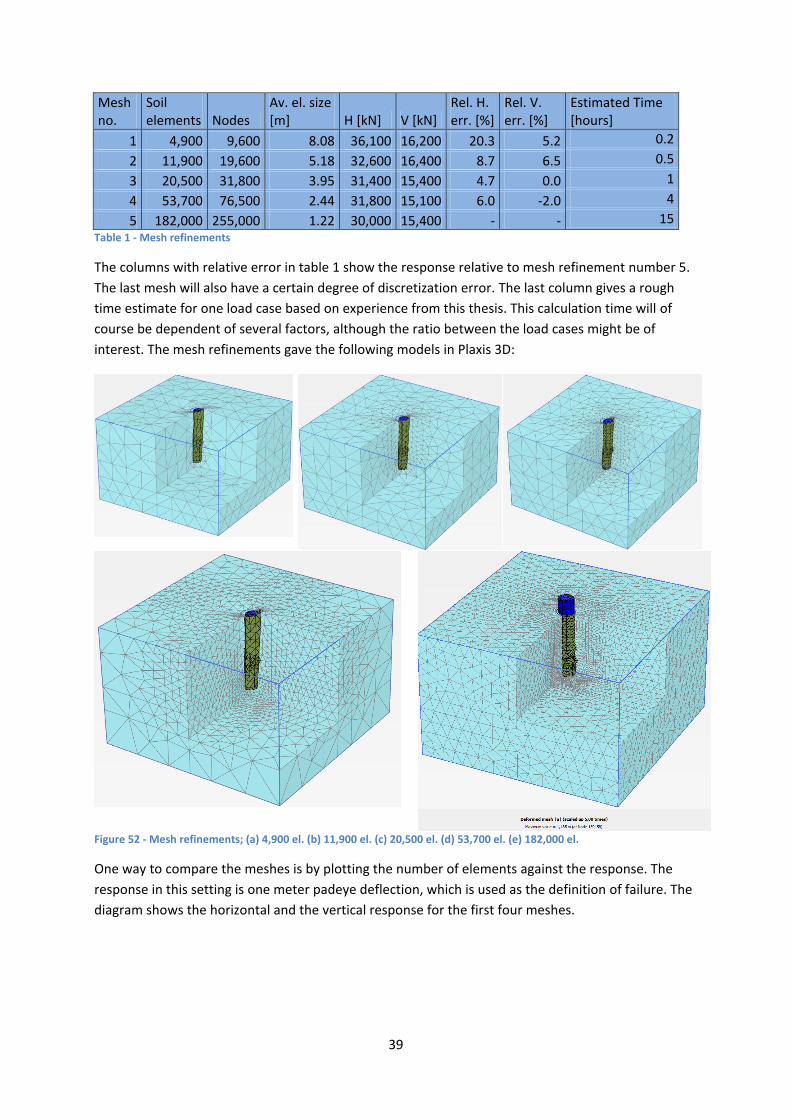
39
Mesh no.
Soil elements Nodes
Av. el. size [m] H [kN] V [kN]
Rel. H. err. [%]
Rel. V. err. [%]
Estimated Time [hours]
1 4,900 9,600 8.08 36,100 16,200 20.3 5.2 0.2
2 11,900 19,600 5.18 32,600 16,400 8.7 6.5 0.5
3 20,500 31,800 3.95 31,400 15,400 4.7 0.0 1
4 53,700 76,500 2.44 31,800 15,100 6.0 -2.0 4
5 182,000 255,000 1.22 30,000 15,400 - - 15 Table 1 - Mesh refinements
The columns with relative error in table 1 show the response relative to mesh refinement number 5.
The last mesh will also have a certain degree of discretization error. The last column gives a rough
time estimate for one load case based on experience from this thesis. This calculation time will of
course be dependent of several factors, although the ratio between the load cases might be of
interest. The mesh refinements gave the following models in Plaxis 3D:
Figure 52 - Mesh refinements; (a) 4,900 el. (b) 11,900 el. (c) 20,500 el. (d) 53,700 el. (e) 182,000 el.
One way to compare the meshes is by plotting the number of elements against the response. The
response in this setting is one meter padeye deflection, which is used as the definition of failure. The
diagram shows the horizontal and the vertical response for the first four meshes.

40
Figure 53 - Convergence - failure load against number of soil elements
It is observed from table 1 and figure 53 that an increase in the number of elements does not change
the response in more than 6% when the number of elements has exceeded 20,000 elements. The
discretization error is however likely to increase with further mesh refinements. During the mesh
refinements, it has been focused on the density of the mesh where the failure mechanisms are likely
to be developed, however in a somewhat smooth sense. This will increase the convergence rate
when it is used in a proper way (Zienkiewicz et. al, 2005). The failure mechanisms will be different
from the horizontal and the vertical load case. For the vertical load case, it is essential to have a large
number of elements close to the base due to the reversed end bearing mechanism. The shaft
resistance will be calculated accurately due to the interface elements. For the horizontal load case
however, it will be important that there are a large number of elements close to the wall. The
meshing options in Plaxis limits the user to control the density regions of the mesh, which means that
some of the refinements favor the horizontal load case more than the vertical, and the other way
around. This is mainly the reason that an increase in elements can increase the discretization error
for a load case. However each mesh refinement will give an overall increased accuracy, which can be
illustrated by averaging the error from the horizontal and the vertical load case. Figure 55 shows the
important locations for a dense mesh due to the specific load case.
Figure 54 - Locations were a dense mesh is required
10000
15000
20000
25000
30000
35000
40000
0 10000 20000 30000 40000 50000 60000
P [
kN]
# elements []
Convergence
P,horizontal(el)
P,vertical(el)

41
5 Results In this chapter, the results will be presented. Based on the results from the mesh refinements, the
model will be based on a mesh consisting of 20,500 soil elements. The results from the combined
loading will be presented first. The combined loading includes 37 load cases, where the direction of
the load vector was changed; both the inclination angle and the torsional angle were varied.
Thereafter, the results from the hand calculation will be presented, followed by the load cases that
correspond to the hand calculations. These analyses will also gain important information to form a
realistic curve-fitting yield surface. Analyses addressing the effect on anchor stiffness will then be
presented; it will be shown that the anchor can be considered rigid. Thereafter, the empirical elastic
stiffness will be determined, and this will be used to form the elastic stiffness matrix of the system.
Load sequences will then be executed, which will determine the plastic behavior due to cyclic two-
way loads. Finally, empirical capacity curves for combined loading will be presented. The objective of
each analysis can be summarized as follows:
Type of analysis Objective Load cases
Failure load at padeye Yield surfaces and deflections 37
Hand calculations Compare against numerical results 6
Failure loads for single-force components Gain information for curve fitting 9
Elastic soil Determine elastic force-displacement
relationship
6
Parametric stiffness anchor Obtain soil-structure interaction 4
Load cycles Gain information regarding elasto-plasticity 3
Figure 55 - Analyses overview
5.1 Combined loading The Plaxis results are based on the model that consists of 20,500 soil elements. Failure was defined
as one meter padeye deflection. 37 load cases were applied, where the difference between the load
cases was the direction of the load vector at the padeye. The following angles were combined:
[ ]
[ ]
Seven different load inclination angles and six different torsional angles were thus used. This results
in 37 load cases, since the vertical load case is independent of the torsional moment; see chapter 4.2.
The following failure loads were obtained for the different load cases:

42
P [kN] β=0 β=5 β=10 β=20 β=45 β=90
α=0 31,400 30,100 27,800 18,300 9,000 6,300
α=10 34,000 33,000 29,700 18,700 9,100 6,400
α=20 36,100 34,600 30,400 19,400 9,500 6,800
α=30 29,700 29,100 26,700 19,700 10,300 7,300
α=45 21,600 21,500 21,000 18,700 12,200 8,900
α=60 17,700 17,700 17,700 17,100 14,400 11,700
α=90 15,400 15,400 15,400 15,400 15,400 15,400 Table 2 - Failure loads from padeye loads
5.1.1 Load-deflection curves
It is important to understand how the system behaves until failure. The load-deflection curves will
therefore be presented. The load-deflection curves are separated in terms of the rotational angle; β.
Figure 56 - Load-deflection curve, β=0 degrees
Figure 56 shows that the highest capacity is obtained when the load inclination angle α is 20 degrees.
The horizontal loads have a well-defined yield plateau, while capacity increases more gradually when
α is more than 30 degrees. It should be noted that Plaxis does not reduce the soil-structure contact
area as the anchor deflects, which implies that the vertical load combinations will be slightly
overestimated.
0
5000
10000
15000
20000
25000
30000
35000
40000
45000
0,0 1,0 2,0 3,0 4,0 5,0 6,0
P [
kN]
Padeye displacement [m]
Force - displacement, β=0o
alpha=0
alpha=10
alpha=20
alpha=30
alpha=45
alpha=60
alpha=90

43
Figure 57 - Load-deflection curve, beta=5 degrees
Figure 57 shows the load combinations with β equals 5 degrees. The load-deformation pattern is
much the same as for β equals 0. The capacity due to torsion is barely reduced.
Figure 58 - Load-deflection, β=10 degrees
Figure 58 shows that the load-deformation pattern is still the same when β is 10 degrees, although
the capacity for horizontal loads has been noticeably reduced due to the induced torsional moment.
Also, the yielding plateau is less prominent.
0
5000
10000
15000
20000
25000
30000
35000
40000
45000
0,0 1,0 2,0 3,0 4,0 5,0 6,0
P [
kN]
Padeye displacement [m]
Force - displacement, β=5o
alpha=0
alpha=10
alpha=20
alpha=30
alpha=45
alpha=60
alpha=90
0
5000
10000
15000
20000
25000
30000
35000
40000
0,0 1,0 2,0 3,0 4,0 5,0 6,0
P [
kN]
Padeye displacement [m]
Force - displacement, β=10o
alpha=0
alpha=10
alpha=20
alpha=30
alpha=45
alpha=60
alpha=90

44
Figure 59 - Load-deflection curve, β=20 degrees
Figure 59 shows that the load-deflection curves were changed, and that the yielding plateau is also
less defined for horizontal loads. The vertical loads are hardly reduced; this is explained by the fact
that when the direction of the force is close to vertical, there is virtually no horizontal component left
to induce a torsional moment.
Figure 60 - Load-deflection curve, beta=45 deg
Figure 60 shows that the horizontal capacity is reduced significantly, clearly governed by the torsional
moment capacity.
0
5000
10000
15000
20000
25000
30000
35000
0,0 1,0 2,0 3,0 4,0 5,0 6,0
P [
kN]
Padeye displacement [m]
Force - displacement, β=20o
alpha=0
alpha=10
alpha=20
alpha=30
alpha=45
alpha=60
alpha=90
0
5000
10000
15000
20000
25000
0,0 1,0 2,0 3,0 4,0 5,0 6,0
P [
kN]
Padeye displacement [m]
Force - displacement, β=45o
alpha=0
alpha=10
alpha=20
alpha=30
alpha=45
alpha=60
alpha=90

45
Figure 61 - Load-deflection curve, β=90 degrees
Figure 61 shows that horizontal loads are further reduced. These results are as expected.
All the load-deflection curves have one common property; the response is first approximately
linearly-elastic prior to yielding. The curves start to yield after about 0.1 m deflection, when the loads
are mobilized at about half of the total capacity. The stiffness in the elastic range seems to be related
to the strength of the load case.
5.1.2 Failure mechanisms
It is necessary to study the failure mode of the system in order to evaluate whether the results are
reasonable. The failure mechanisms from the analyses where the torsional angle is 0 will be
presented. Failure mechanisms will be visualized by incremental strains and incremental
displacements for chosen load cases.
0
5000
10000
15000
20000
25000
0,0 1,0 2,0 3,0 4,0 5,0 6,0
P [
kN]
Padeye displacement [m]
Force - displacement, β=90o
alpha=0
alpha=10
alpha=20
alpha=30
alpha=45
alpha=60
alpha=90

46
Incremental strains
Figure 62 - Incremental strains, β=0 degrees: (a) α=0 degrees, (b) α=20 degrees, (c) α=45 degrees, (d) α=90 degrees
When the inclination angle is increased from 0 to 20 degrees, the soil at the base mobilizes, and a
larger capacity is obtained. When the inclination angle is 45 degrees, the failure mechanism is
vertical, with a reversed end-bearing capacity being obtained. The mechanisms at inclination angles
of 45 and 90 degrees are identical.

47
Incremental displacements
Figure 63 - Incremental disp., β=0 degrees: (a) α=0 degrees, (b) α=20 degrees, (c) α=45 degrees, (d) α=90 degrees
The same conclusions hold true for the incremental displacements as for the incremental shear
strains.

48
Incremental displacements anchor, β=0 degrees
Figure 64 - Incremental displacements anchor,β=0: (a) α=0, (b) α=10, (c) α=20, (d) α=30, (e) α=45, (f) α=60, (g) α=90
Another way of visualizing the failure modes is to isolate the anchor from the soil in the output. The
failure modes in terms of incremental displacements of the anchor for the inclination angles between
0 and 90 degrees when β=0 is shown is figure 64. It shows the same characteristics observed
previously.
5.1.3 Failure surfaces in two dimensions
The results from the load cases can be plotted in several ways, with the horizontal-vertical load space
being commonly used. The horizontal component of the force vector is plotted against the vertical
force component. In the following ,a HV space with different torsional angles will be shown, which
means that it is actually a HVβ-space, see figure 65.
Figure 65 - HV space
0
2000
4000
6000
8000
10000
12000
14000
16000
18000
0 5000 10000 15000 20000 25000 30000 35000 40000
V [
kN]
H [kN]
HV-space
beta=0
beta=5
beta=10
beta=20
beta=45
beta=90

49
Each point of the curves represent a failure state, given in table 2. The HV space shows several
interesting tendencies. Firstly, it shows how a torsional angle will reduce the capacity of the system.
When the angle β is 5 degrees, the capacity is almost unchanged, but when β increases, the capacity
suddenly drops. Secondly, it can be seen that when the inclination angle α increases from 0, the
horizontal capacity also increases. This can be explained as follows: Even though the results are
presented in the HV space, there are other force components as well; namely the bending moments
and the torsional moment. It turns out that when you load the system with an incremental vertical
load, you will also unload the system of bending moments, if the horizontal component dominates.
This will be further explored in section 5.5. Finally, we see that all the β curves intersect when α is 90
degrees. Again, this is because the horizontal component of the force vector dissipates, and there is
no horizontal force left to cause torsion.
In order to see how much the torsional angle β reduces the capacity, it may be convenient to plot the
inclination angle α against the failure load. Figure 66 shows how the failure load depends on the
inclination angle α, and the torsional angle β. The failure load tendencies in the figure correspond to
those of the other figures.
Figure 66 - Failure load P with the angles alpha and beta
If the chosen definition of failure is a 5-meter padeye deflection, the following HV space would be
obtained:
0
5000
10000
15000
20000
25000
30000
35000
40000
0 15 30 45 60 75 90
P [
kN]
α [deg]
Failure load
beta=0
beta=5
beta=10
beta=20
beta=45
beta=90

50
Figure 67 - HV space, failure defined as 5 m deflection
Figure 67 shows the HV space where failure is defined as a 5-meter deflection at the padeye. The
vertical forces increased significantly from the HV space where failure was defined as 1-meter
padeye deflection, while the change in horizontal capacity is less marked. The shapes of the different
HV spaces are much the same.
Capacity curves with other deformation criteria with no torsion are also shown.
Figure 68 - Yield surface in HV space; deflection criteria: 0.2 m, 0.4 m, 0.6 m, 0.8 m and 1 m
0
5000
10000
15000
20000
25000
0 5000 10000 15000 20000 25000 30000 35000 40000
V [
kN]
H [kN]
HV space, 5 m
beta=0
beta=5
beta=10
beta=20
beta=45
beta=90
0
2000
4000
6000
8000
10000
12000
14000
16000
18000
0 10000 20000 30000 40000
V [
kN]
H [kN]
HV space; yield surfaces
d=0,2m
d=0,4m
d=0,6m
d=0,8m
d=1,0m

51
5.1.4 Three-dimensional plots
Since the force vector applied at padeye consists of three independent components, see equations
4.8-4.15, the response can be visualized in the space with three components as well. One option
might be to transform components into the HVT-space, which consist the total horizontal, vertical
and torsional load components. H and V are already given, while T is simply H multiplied by sin(β)
times ex, where ex is the eccentricity between the neutral axis and the load attachment point. The
results can also be plotted directly in the HxHyV-space, where Hx is the decomposed horizontal load in
the x-direction and Hy is the decomposed horizontal load in the y-direction.
Another option is to plot the failure load P as a function of the angles α and β, see figure 69.
Figure 69 and 70 has showed that the response can be visualized in by three-dimensional plots, but
that it may be more difficult to interpret the tendencies.
Figure 69 - HxHyV space
Figure 70 - P-αβ-space

52
5.2 Hand calculations It is important to estimate the results from a numerical study by hand calculation in order to ensure
that the numerical analyses are reasonable. The predictions should ideally be made prior to the
analyses, in order to avoid adjustments in the hand calculations to get a good match. It is also
important that the hand calculations use the same parameters as the numerical model. The hand
calculations in this section include the ultimate force components of the anchor and the horizontal
and vertical stiffness. Due to symmetry, neglecting the effects from the padeye, there are a total of
four force components that need to be determined; the horizontal, the vertical, the bending moment
and the torsional moment capacity.
5.2.1 Horizontal capacity
According to Randolph et al. (1998), the horizontal capacity can be estimated by figure 71:
(5.1)
Figure 71 - Horizontal capacity (Randolph, 1998)
Figure 72 - Factor flow-around mechanism (Martin & Randolph, 2006)
Randolph & Gourvenec (2011) state that the flow-around mechanism will be developed close to the
surface for soil with linearly increasing strength, and that the mechanism can be assumed to apply
for the whole pile, since the soft soil at the seabed contributes little support. Figure 72 gives a value
of 10.8 with a roughness factor α = 0.44. In this approach, the base shear also has to be included. The
following capacity is then obtained:
(
)
(5.2)
Finally, the method of Aubeny & Murff (2005) will be presented. The base shear also had to be
included in this case. The calculations are spreadsheet friendly, and are prepared in Excel with small
depth increments (Δz=0.1 m, 300 increments). A spreadsheet with larger increments is attached for
illustration. The method gave a capacity of H=32,300 kN. The following diagrams were obtained:

53
Figure 73 - Diagrams for the suction anchor
Three different ways of calculating the horizontal capacity have now been executed. The results were
almost the same; between 32,300 kN and 34,000 kN.
5.2.2 Vertical capacity
The maximum vertical pull-out capacity can be calculated by many methods. However, most
methods will not capture the coefficients that are used for this project. The limit equilibrium where
the anchor is treated as a pile is a good way to estimate the capacity. The equilibrium in the
undrained condition gives:
(5.3)
The weight of the anchor is the following:
∑
(
)
(5.4)
The effective weight of the anchor is taken as:
-30
-25
-20
-15
-10
-5
0
0 2 4 6 8 10 12
Me
ters
fro
m t
he
se
abe
d [
m]
Value Nps
Nps
Nps
-35
-30
-25
-20
-15
-10
-5
0
0 1000 2000 3000
Me
ters
fro
m t
he
se
abe
d [
m]
Strip load q [kN/m]
Strip load
q(z)
-30
-20
-10
0
-30000 -20000 -10000 0 10000 20000
Me
ters
fro
m t
he
se
abe
d
[m]
Shear force [kN]
Shear diagram
V(z)
-30
-25
-20
-15
-10
-5
0
0 50000 100000 150000
Me
ters
fro
m t
he
se
abe
d
[m]
Moment [kNm]
Moment diagram
M(z)

54
(5.5)
The reverse end-bearing capacity factor NC is taken as 9, which should be a conservative value for the
given input parameters. See chapter 3.2.2 for more details. The undrained shear strength is taken at
base level. The following capacity is obtained:
(5.6)
If the chosen value of Nc was taken as 12, the capacity would be 16,700 kN. The calculated vertical
capacity is thus 14,000 kN, but a higher capacity is expected in the model. The reverse end-bearing
capacity for this anchor represents about half of the total capacity.
5.2.3 Bending moment capacity
The bending moment capacity is calculated from the limit equilibrium where the lateral forces acting
on the suction anchor are treated as a linearly increasing strip load. This leads to the following
bending moment capacity:
∑ (5.7)
∑ (5.8)
⇒
(
)
0.2 (5.9)
If the horizontal capacity is taken as 34,000 kN, the ultimate bending moment will be 204,000 kNm.
Since the bending moment capacity is only dependent on the horizontal capacity, the discretization
error is likely to be approximately the same. However, it is unlikely that the limiting earth pressure
will be fully mobilized close to the rotation center. On the other hand, the shear forces at the
interfaces might also add a small portion to the bending moment capacity.
5.2.4 Torsional capacity
The torsional capacity will also be estimated from the limit equilibrium. Three factors contribute to
the capacity; the shaft resistance, the base resistance and the resistance due to the padeye. This
leads to the following expression:
(5.10)
The last term relates to the padeye modeled as a plate. The bearing capacity factor for a plate due to
the flow-around mechanism can be taken as 12.5, which is typical for drag anchors (Randolph &
Gourvenec, 2011). The eccentricity; ex, is the distance between the neutral axis and the resultant
force from the plate, taken as 3.5 meters. Inserting these values gives:
(5.11)
The estimated torsional capacity is thus 16,000 kNm.

55
5.2.5 Stiffness
The vertical stiffness is first calculated in accordance
with Paulos and David (1974). The height of the model
is 50 meters, while the length of the pile is 30 meters,
which gives a height-to-length ratio equal to 1.67. This
gives an influence factor; Iρ, equal to 0.7, while the
influence factor would be 1.1 if the model had an
infinite depth. It should be noted that the method
assumes constant stiffness, while the stiffness in the
model is almost proportional to depth. An average
stiffness over the pile length is applied. The following
stiffness is obtained with this method:
(
)
(5.12)
The fact that the method is based on a constant stiffness makes the method less comparable to the
model. The method of Randolph & Gourvenec (2011) takes stiffness changes into account, and is
thus better suited. The stiffness of the pile is divided into the shaft stiffness and the base stiffness,
which behave like additive springs. The following stiffness is obtained:
(5.13)
where is an influence parameter for the size of the soil volume, often taken as 4
is the radius of the pile at the pile base
is the shear stiffness at the pile base
Insertion gives a value =157,000 kN/m.
The horizontal stiffness is calculated by using the formula presented in chapter 3.2.2:
(5.14)
The horizontal stiffness is thus 204,000 kN/m.
5.2.6 Summary of the hand calculations
Hand calculations on both strength and stiffness have now been performed. The results will be used
to evaluate the reliability of the numerical results. The hand calculations showed the following
results:
Figure 74 - Influence factor axially loaded pile (Poulos & David, 1974)

56
Horizontal capacity 32,300 kN – 34,000 kN
Vertical capacity 14,000 kN
Bending moment capacity 194,000-204,000 kNm
Torsional moment capacity 16,000 kNm
Horizontal stiffness 204,000 kN/m
Vertical stiffness 157,000 kN/m
Table 3 - Results from hand calculations
5.3 Single-force components with Plaxis 3D In order to calculate the ultimate force components of the anchor, separate analyses were executed,
where each load component was loaded separately. Due to the constraint relations of the loads, the
single-force components were represented with a set of load vectors, where the resultant force
intersected with the three neutral planes in space; load vectors applied at the padeye will result in six
force components, and it is not possible to isolate the individual components. Two of the neutral
planes are known prior to analyses, due to symmetry, while the eccentricity between the padeye and
the neutral plane in the z-direction; ez, needs to be obtained. Failure was defined as one meter
padeye deflection. The results from these analyses will provide important information, which will be
used to construct a realistic failure surface, and will also be used for comparison with the hand
calculations.
The first step required is to determine the neutral axis of the anchor. Due to symmetry, the neutral
axis in the xz-plane and the yz-plane will intersect in the middle of the cylinder. This gives an
eccentricity to the load attachment point in the x-direction of 3.75 meters, while there is no
eccentricity in the y-direction; ex=3.75 m, ey=0. The definition of the neutral axis in the xy-plane in
this context is the plane that induces no bending moment due to horizontal loads. Since horizontal
loads in this plane will not produce any bending moment, the largest horizontal capacity will be
obtained in this plane. This property can be exploited; the loading plane can be changed until the
largest capacity is obtained. The loading plane has been lowered by combining a horizontal load at
the padeye with a bending moment, represented by coupled forces. The eccentricity from the
padeye will then be ez=M/H. Firstly, four load cases where applied; namely ez=M/H=2.25 m, 3.0 m,
3.75 m and 4.5 m. The following load-deflection curves were obtained:

57
Figure 75 - Parametric study of ez
It is seen that 3 meter eccentricity will result in the largest capacity. The second largest was the load
case where the eccentricity was 2.25 meters. Further analyses with eccentricities of 2.50 meters and
2.75 meters were then executed, in order to determine the eccentricity in greater detail. However,
an eccentricity of 3 meters was still the load case that gave the largest capacity. Selected failure
mechanisms from the analyses will be shown:
Horizontal load, z=2.25 meters Horizontal load, z=2.5 meters
0
5000
10000
15000
20000
25000
30000
35000
40000
45000
50000
0,0 1,0 2,0 3,0 4,0 5,0 6,0
P [
kN]
Padeye displacement [m]
Load deflection, ez
z=4,5m
z=3,75m
z=3,0m
z=2,25m
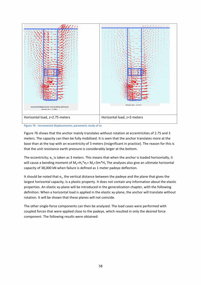
58
Horizontal load, z=2.75 meters Horizontal load, z=3 meters
Figure 76 - Incremental displacements; parametric study of ez
Figure 76 shows that the anchor mainly translates without rotation at eccentricities of 2.75 and 3
meters. The capacity can then be fully mobilized. It is seen that the anchor translates more at the
base than at the top with an eccentricity of 3 meters (insignificant in practice). The reason for this is
that the unit resistance earth pressure is considerably larger at the bottom.
The eccentricity; ez, is taken as 3 meters. This means that when the anchor is loaded horizontally, it
will cause a bending moment of My=Hx*ez= My=3m*Hx The analyses also give an ultimate horizontal
capacity of 38,000 kN when failure is defined as 1 meter padeye deflection.
It should be noted that ez, the vertical distance between the padeye and the plane that gives the
largest horizontal capacity, is a plastic property. It does not contain any information about the elastic
properties. An elastic xy-plane will be introduced in the generalization chapter, with the following
definition: When a horizontal load is applied in the elastic xy-plane, the anchor will translate without
rotation. It will be shown that these planes will not coincide.
The other single-force components can then be analyzed. The load cases were performed with
coupled forces that were applied close to the padeye, which resulted in only the desired force
component. The following results were obtained:

59
Figure 77 - Load-deflection curves
Figure 77 shows the load-deflection curves from the load cases that have only one force component.
The deflections are still measured at the padeye. Note that the bending moment in the figure is
divided by the diameter D=6 m and that the torsional moment is divided by 1 meter. This is done to
achieve the same dimensions and values in the same range. The bending moment was about the y-
axis. It is assumed that the moments and the horizontal forces had the same capacity in the x- and
the y-direction, due to the minor impact of the padeye geometry. The ultimate capacity is defined as
the load that causes 1-meter padeye deflection.
The results from the force component analyses can be summarized as follows:
Description Symbol label value
Distance in the x-direction from the padeye to the neutral
axis
ex [m] 3.75
Distance in the y-direction from the padeye to the neutral
axis
ey [m] 0
Distance in the z-direction from the padeye to the plastic
neutral axis
ez [m] 3
Ultimate horizontal force Hu =Hx,u=Hy,u [kN] 38,000
Ultimate vertical force Vu [kN] 15,500
Ultimate bending moment Mu =Mx,u=My,u [kNm] 230,000
Ultimate torsional moment Tu [kNm] 23,800
Table 4 - Eccentricities and ultimate forces
0
5000
10000
15000
20000
25000
30000
35000
40000
45000
50000
0,000 1,000 2,000 3,000 4,000 5,000 6,000
Re
spo
nse
[kN
]
u [m]
Reaction, ult
M/D
T/1m
V
Hopt

60
The ultimate capacities can be compared to the combined loading analyses. An inclination angle; α,
and a torsional angle; β, of 0 gave a capacity of 314,00 kN, while the ultimate horizontal capacity is
38,000 kN. Because of the plastic eccentricity of 3 meters, the capacity will be reduced by about 17%.
For that load case, the mobilization factor of the bending moment was
f=31,400kN*3m/230,000kNm=41%. The vertical load case gave a capacity of 15,400 kN, while the
ultimate vertical capacity was 15,500 kN. This means that the influence of the 3.75 meter eccentricity
due to vertical loads can in practice be neglected. The mobilization factor for the bending moment of
the vertical load case was f=15,400kN*3.75m/230,000kNm=25%. An angle α of 0 and an angle β of
90 degrees give a capacity of 6,300 kN. This gives a torsional moment of
T=6,300kN*3.75m=23,600kNm, while the ultimate torsional moment is 23,800 kNm. This means that
the capacity for this load case is totally governed by the torsional capacity.
5.4 Stiffness of the anchor One assumption that is often made during suction anchor calculations is that the anchor is rigid. The
soil-structure interaction will then be quite simple, and forces can then be transposed to force
components without any simplification. Analyses that study the relation between the stiffness of the
anchor and the load-deflection curve have been carried out, in order to check if the assumption is
reasonable. Four load cases have been performed, with the difference between each load case being
the E-modulus to the anchor. The force vector is horizontal, and is applied at the padeye.
The E-modulus is the following for the different load cases:
Load Case 1 E1 [MPa] Esteel*10-4 21
Load Case 2 E2 [MPa] Esteel*10-2 2,100
Load Case 2 E3 [MPa] Esteel 210,000
Load Case 4 E4 [MPa] Esteel*102 21,000,000
Table 5 - E-modulus load cases
This resulted in the following force-displacement curves:

61
Figure 78 - Load-displacement curve parametric stiffness
Figure 78 shows how the soil response depends on the stiffness of the structure. Load Case 3 has the
original stiffness. If the Young’s modulus is increased 100 times, the response is more or less exactly
the same. This implies that the system can be assumed to be rigid. The figure shows that if the
Young’s modulus was decreased 100 times, the soil-structure interaction would become important. It
is interesting to note that when the padeye deflection increases, the capacity is almost the same as
for the original load case. When E is reduced 10,000 times, most of the capacity at practical
displacements has dissipated.
5.5 Elastic soil response The elastic soil response is needed for the elasto-plastic formulation, and will in addition give
information about expected deflections due to small loads. It will be shown that a linearly-elastic
response can be assumed for loads until the mobilization degree f=0.6 is reached. Further loading will
cause plastic deflection and a hardening law is needed. Plastic deformations will be covered in the
next chapter; elasto-plasticity.
The stiffness matrix in the exercise is obtained by force-displacement relations at the padeye. Three
separate orthogonal forces are applied at the padeye, and the corresponding padeye displacements
are measured. The set of orthogonal forces comprises Hx, Hy and V; the two horizontal forces and the
vertical force, respectively. The relations will give the flexibility matrix, and the stiffness matrix can
easily be obtained by inversing the flexibility matrix. The flexibility coefficients are determined by
empirical curve fitting to the associated load-deflection curves; the elastic part is predicted as the
part of the load-deflection curves with a linear behavior, and intersects the load-deflection curves
when the mobilization factor are 0.6. The stiffness can then be regarded as an secant modulus.
Deflection in the x-direction due to the orthogonal load cases:
0
5000
10000
15000
20000
25000
30000
35000
40000
0,0 1,0 2,0 3,0 4,0 5,0 6,0
P [
kN]
u [m]
P-u, stiffness
Load Case 4
Load Case 3
Load Case 2
Load Case 1

62
Figure 79 - Load deflection; deflections measured in the x-direction
Deflection in the y-direction due to the orthogonal load cases:
Figure 80 - Load deflection; deflection measured in the y-direction
Deflection in the z-direction due to the orthogonal load cases:
0
5000
10000
15000
20000
25000
30000
35000
-0,1 0,0 0,1 0,2 0,3
P [
kN]
ux [m]
Load deflection, deflection in the x-direction
Hx-ux
Stiffness Hx-ux
V-ux
stiffness V-ux
Hy-ux
stiffness Hy-ux
0
5000
10000
15000
20000
25000
30000
35000
-0,1 0,0 0,1 0,2 0,3
P [
kN]
uy [m]
Load deflection, deflection in the y-direction
Hx-uy
Stiffness Hx=uy
V-uy
stiffness V-uy
Hy-uy
stiffness Hy-uy

63
Figure 81 - Load deflection; deflection measured in the z-direction
The empirical elastic curves correspond to the load-deflection curves in a proper way for small loads;
the assumption of an initial elastic behavior is thus appropriate. The yielding starts to affect the load-
deflection curves when the mobilization factor; f, is approximately 0.6 for all the orthogonal load
cases. The yielding plateau in the load-deflection curves is prominent for all directions. The following
flexibility matrix is obtained by curve fitting:
[ ]
[
]
(5.15)
The stiffness matrix of the system is found by inverting the flexibility matrix:
[ ] [
]
(5.16)
The stiffness matrix is important for the elasto-plastic formulation and for the dynamical response of
the system. The stiffness of the foundation will have an impact on the eigenfrequencies of the
platform. For simplicity, assume that the suction anchor is the foundation for a tension leg platform
in 500-meter deep waters. The stiffness of the cable can be approximated as kcable=EA/L. Appropriate
dimensions give a vertical cable stiffness of about 40,000kN/m. The stiffness of the system due to the
stiffness of the foundation will then be and
a change in the vertical eigenfrequency of 14 percent. In other words, the stiffness of the foundation
does have a significant impact on the dynamical response and should be accounted for.
5.6 Load cycles Cycles of elasto-plastic loads have been executed in order to gain information about realistic elasto-
plastic behavior. Three different load-case histories have been performed; one in each of the x-, y-
0
5000
10000
15000
20000
25000
30000
35000
-0,1 0,0 0,1 0,2 0,3
P [
kN]
uz [m]
Load deflection, deflection in the z-direction
Hx-uz
stiffness Hx-uz
V-uz
stiffness V-uz
Hy-uz
stiffness Hy-uz

64
and z-directions. Firstly, the anchor was loaded to a mobilization factor f=0.9, then unloaded again
until f=0.9, and finally reloaded to f=0.9. The following results were obtained:
Figure 82 - Loads and deflections in the x-direction
Figure 83 - Loads and deflections in the y-direction
Figure 84 - Loads and deflections in the z-direction
-30000
-20000
-10000
0
10000
20000
30000
-0,4 -0,2 0,0 0,2 0,4
Hx
[kN
]
ux [m]
Hx-ux
Hx-ux
-8000
-6000
-4000
-2000
0
2000
4000
6000
8000
-0,6 -0,4 -0,2 0,0 0,2 0,4 0,6
Hy-uy
Hy-uy
-15000
-10000
-5000
0
5000
10000
15000
20000
-1,0 -0,5 0,0 0,5 1,0
V [
kN]
uz [kN]
V-uz
V-uz

65
The loading cycles in all directions show the same tendency; namely that the loading cycles form a
closed loop and that the Bauschinger effect is present. This imposes kinematic hardening rather than
isotropic hardening. The material properties at element level is modeled as elastic-perfectly plastic,
which means that the yield surface will not expand during loading. It is thus reasonable that the yield
surface neither will expand at a global level, only translate. However, the system cannot be subjected
to a compression force in reality, since the mooring chain is not capable of transferring tensile loads.
Isotropic hardening is also more commonly applied.
Also note that the compression force in the vertical load cycle is less than the tensile force. This is
because the weight of the anchor reduces the compression capacity, while it will increase the tensile
capacity.
5.7 Curve-fitting yield surfaces Two different curve-fitting yield surfaces will be presented in this section. The difference between
them is how the bending moment is included. The second formula has a better physical foundation,
and also provides the most accurate results. For this specific problem it is required that the curve-
fitting formula cooperates with all 6 force components that will be presented during a general load at
the padeye. However, since the force components are constant to each other, it will still be possible
to plot the curve-fitting formula in 3 dimensions. The yield surfaces will then be determined in terms
of loads applied at the padeye.
5.7.1 The first curve-fitting yield surface
The first curve is based on the following formula:
(5.17)
where Hx is the horizontal force in the x-direction
Hy is the horizontal force in the y-direction
V is the vertical force
Mx is the bending moment about the x-axis
My is the bending moment about the y-axis
T is the torsional moment
Hu is the ultimate horizontal force in the y-direction, equal to 38,000 kN
Vu is the ultimate vertical force, equal to 15,500 kN
Mu is the ultimate bending moment about the y-axis, equal to 230,000 kNm
Tu is the ultimate torsional moment capacity
a, b, c, d are curve-fitting constants
The coefficient a relates to both horizontal components and the coefficient d relates to both bending
moments components, due to symmetry. It is thus only four coefficients that determine the surface.
The moments can then be eliminated due to the constraints by using equations 4.11-4.13:
| |
(5.18)
The equation can also be presented in terms of P, α and β by applying equations 4.10-4.13:

66
| |
(5.19)
The latter expression is useful in order to determine the magnitude of the force vector for given
angles. This can for instance be done by Newton's iterations (Kreyszig, 2006):
(5.20)
where:
| |
(5.21)
It is important to have sufficient iterations to ensure convergence of the empirical surface. The
following error tolerance has been applied:
|
| (5.21)
Optimization of the empirical coefficients can be achieved by the method of least squares (Kreyszig,
2006). Conservative adjustments can then be made manually. The following values for the
coefficients were obtained at the end:
Coefficient Value
a 3
b 5
c 1
d 4
Table 6 - Empirical coefficients
The empirical yield surface will be plotted against the Plaxis results after the second empirical yield
surface is presented.

67
5.7.2 The second curve-fitting yield surface
The second curve-fitting formula uses the following formula:
( ( )
)
( ( )
)
(5.22)
where Hx is the horizontal force in the x-direction
Hy is the horizontal force in the y-direction
V is the vertical force
Mx is the bending moment about the x-axis
My is the bending moment about the y-axis
T is the torsional moment
Hu is the ultimate horizontal force in the y-direction, equal to 38,000 kN
Vu is the ultimate vertical padeye force, equal to 15,400 kN
Mu is the ultimate bending moment about the y-axis, equal to 230,000 kNm
Tu is the ultimate torsional moment capacity
a, b, c, d are curve-fitting constants
The difference between the empirical yield surfaces is how the formulas interact with the bending
moments. Since the pile can be considered rigid, a constraint relation between bending moments
and translational forces can be expressed analytically if the earth pressure resistance can be
expressed as a function. Due to the strength profile, the earth pressure per unit length can be
approximated as linearly increasing; see chapter 5.2. The limit strip load can be simplified as follows:
(5.23)
The simplified strip load and the calculated strip load can be compared (the base shear is distributed
to the last pile meter):
Figure 85 - Strip load; hand calculated and simplified
-30
-25
-20
-15
-10
-5
0
0 500 1000 1500 2000 2500 3000
z [m
]
q [kN/m]
Strip load
hand calculated
simplified

68
The analytical expression is obtained by solving the three equations below. The equations are based
on the limit equilibrium, and exploit the property that the external moment can be expressed as the
resultant force multiplied by the projected distance from the neutral point (where the three plastic
planes intersect):
∑ (5.24)
∑ (5.25)
(5.26)
The eccentricity e, in the third equation denotes the distance between the horizontal neutral plane
and the resultant force.
Equilibrium of the horizontal forces gives the following expression:
(5.27)
A non-dimensional earth pressure-to-length ratio is introduced:
(5.28)
The expression can then be simplified as:
(5.29)
Equilibrium of the bending moment gives the following expression:
(
)
(5.30)
The expression can be rewritten as:
(5.31)
Applying the third equation and introducing the non-dimensional eccentricity factor; n=e/L, gives:
(5.32)
This third-degree equation can be solved when the eccentricity; z, is known. There are three
solutions, where only one of the roots is of interest. The reduced horizontal capacity, due to the
moment, is given by equation 5.29, where l is given of equation 5.32. This rather complicated
expression is difficult to implement, and a simplified empirical formula would be beneficial. It turns
out, after several trial functions, that the equation is very similar to the following expression:
(
)
(5.33)
69
The analytical expression can be plotted against equation 5.33, with different values of d being
chosen; 1, 1.5 and 2.
Figure 86 - Reduction due to padeye position
This relation will make the interaction between the force components more physical, and will
increase the accuracy.
The moments in the yield surface can be eliminated through equations 4.11-4.13:
( (| |
)
)
( (
)
)
(5.34)
The equation can further be presented in terms of P, α and β by applying equations 4.10-4.13:
( ( | |
)
)
( (
)
)
(5.35)
This expression will be used in order to determine the magnitude of the force vector for given angles.
This can for instance be done by Newton's iterations, see equation 5.20. The yield surface 2 has the
following expression:
0,0
0,1
0,2
0,3
0,4
0,5
0,0 0,2 0,4 0,6 0,8 1,0
n=z
/L
Hreduced/Hu
Reduction due to moment
analytical
d=1
d=1.5
d=2

70
( ( | |
)
)
( (
)
)
(5.36)
The same error tolerance has been applied for the second yield surface, see equation 5.21. The
denominator in the horizontal load part decreases when the moment increases; this will effectively
reduce the horizontal capacity. It is seen from Plaxis results that the moment does not significantly
reduce the vertical capacity, and it is therefore not included in the equation due to its complexity.
However, the vertical capacity in the equation is replaced by the vertical capacity with respect to
padeye loading; 15,500kN is replaced by 15,400kN. This means that the vertical loading term
indirectly includes the interaction with the bending moment.
The method of least squares is applied in order to obtain the best curve fitting for the empirical
coefficients (Kreyszig, 2006). Adjustments are then applied to make the surface slightly more
conservative. The following values were obtained:
Coefficient Value, optimized: accuracy=99.35% Value, modified: accuracy=99.30%
a 5.5 5
b 4.8 5
c 2.1 2
d 2.0 2
Table 7 - Empirical coefficients
Yield surfaces against Plaxis results
The two different yield surfaces will be compared to the Plaxis results. The yield surfaces will then be
discussed briefly.
Figure 87 - Yield surfaces, β=0 degrees
0
2000
4000
6000
8000
10000
12000
14000
16000
18000
0 10000 20000 30000 40000
V [
kN]
H [kN]
β=0o
Plaxis3D
crurve fitting 2
Curve fitting 1

71
Figure 87 shows the results from Plaxis against both empirical formulas when is 0 degrees. Both
empirical yield surfaces intersect most load cases quite well, although the first curve-fitting formula
underestimates, in particular, the load case when the inclination angle; α, is 20 degrees. It also has
one limitation; when α increases from 60 to 90 degrees, the curve suggests that the vertical capacity
will be reduced due to an increasing moment. However, the results from Plaxis suggest that this
additional moment has a negligible impact on the vertical capacity.
Figure 88 - Yield surfaces, β=5 degrees
Figure 88 shows the yield surfaces when the torsional angle is 5 degrees. Both empirical curves fit
well with the Plaxis results, although the second empirical curve fits better. Both curves overestimate
the horizontal load case by about 2%.
Figure 89 - Yield surfaces, β=10 degrees
Figure 89 shows the yield surfaces when the torsional angle β is 10 degrees. The first empirical curve
underestimates the horizontal load cases by a few percent. The second curve has a good curve fit.
0
2000
4000
6000
8000
10000
12000
14000
16000
18000
0 10000 20000 30000 40000
V [
kN]
H [kN]
β=5o
Plaxis3D
curve fitting 2
curve fitting 1
0
2000
4000
6000
8000
10000
12000
14000
16000
18000
0 5000 10000 15000 20000 25000 30000 35000
V [
kN]
H [kN]
β=10o
Plaxis3D
curve fitting 2
Curve fitting 1

72
Figure 90 - Yield surfaces, β=20 degrees
Figure 90 shows that the first empirical yield surface does not have the same shape as the Plaxis
results, although the second empirical yield surface fits well.
Figure 91 - Yield surfaces, β=45 degrees
0
2000
4000
6000
8000
10000
12000
14000
16000
18000
0 5000 10000 15000 20000
V [
kN]
H [kN]
β=20o
Plaxis3D
curve fitting 2
Curve fitting 1
0
2000
4000
6000
8000
10000
12000
14000
16000
18000
0 2000 4000 6000 8000 10000
V [
kN]
H [kN]
β=45o
Plaxis3D
curve fitting 2
Curve fitting 1

73
Figure 92 - Yield surfaces, β=90 degrees
Figure 91 and figure 92 show that both curve-fitting surfaces correspond well with the Plaxis results.
It can be concluded that the second curve-fitting yield surface corresponds better with the Plaxis
results. This applies to both the shape of the curve and the accuracy for all values of the angle β.
From the method of least squares, the average error of the curve fitting caused by the load cases was
0.70%. This means that for an arbitrary load case, the difference between the failure load from Plaxis
and the corresponding point from the empirical surface is expected to be 0.70%. In other words, the
second curve-fitting formula interpolates the results almost perfectly.
Both empirical formulas consist of four empirical coefficients, although the latter formula is more
comprehensive. This is especially prominent due to differentiation, which is required because of
Newton's iterations and the implementation of the elasto-plastic formulation due to the flow rule.
However, the second curve-fitting formula is definitely not too complicated to implement.
The results from the second yield surface are plotted against the Plaxis results in isolation, to show
the accuracy:
0
2000
4000
6000
8000
10000
12000
14000
16000
18000
0 1000 2000 3000 4000 5000 6000 7000
V [
kN]
H [kN]
β=90o
Plaxis3D
curve fitting 2
Curve fitting 1

74
Figure 93 - Plaxis results versus yield surface 2
0
2000
4000
6000
8000
10000
12000
14000
16000
18000
0 10000 20000 30000 40000
V [
kN]
H [kN]
Plaxis results vs yield surface 2
beta=0,plaxis
beta=5,plaxis
beta=10,plaxis
beta=20,plaxis
beta=45,plaxis
beta=90,plaxis
beta=0
beta=5
beta=10
beta=20
beta=45
beta=90

75
6 Elasto-plastic formulation The elasto-plastic formulation will be presented in this chapter. The first section will be devoted to
the formulation due to padeye loads and deflections, while the implementation and how to use the
formulation will be the focus towards the end of the chapter. The theory applied uses a formulation
with respect to stresses and strains. The formulation given in this chapter will be adopted in terms of
displacements and loads at the padeye.
6.1 Formulation Elastic and plastic deformation might take place during a load step. How much the elastic and plastic
deformation contribute, and how the mobilization and stiffness change, are described by an elasto-
plastic formulation. An elasto-plastic formulation requires several elements (Cook et. al, 2001):
Compatibility
Stiffness matrix
Yield criterion
Flow rule
Hardening rule
These elements are used to trace the displacements, control yielding and the tangential stiffness of
the system. Each element will be dealt with separately. How to put the elements together, is also
discussed.
6.1.1 Compatibility
Compatibility simply states that the total displacements are equal to the sum of the elastic and the
plastic displacements (Cook et. al, 2001):
{ } { } { } (6.1)
After a load step, the displacement vectors will be updated:
{ } { } { } (6.2)
{ } { }
{ } (6.3)
{ } { } { } (6.4)
6.1.2 Stiffness and flexibility matrixes
The stiffness and flexibility matrixes are already obtained, see equations 5.15 and 5.16. The flexibility
matrix controls the elastic deflections, while the stiffness matrix shows the stiffness behavior of the
system. Elastic deflections are governed by the following equation:
{ } {
} [ ] { }
[
]
{
}
(6.5)

76
6.1.3 Yield criterion
The yield criterion defines how the system yields. Two different yield formulas have already been
presented in section 5.7. When the state parameter f is inserted, the yield criterion is complete. The
state parameter has an initial value. If the expression is less than 0 it implies that the plastic criterion
is not fulfilled, and only elastic response takes place. Two yield criterions will be presented. The first
one has the following expression:
(6.6)
And the second one is given of:
( (
)
)
( (
)
)
(6.7)
If compression force applied to the padeye also will be present, absolute signs will be needed for
each force component, and is thus implemented in the spreadsheet. Eliminating the moments
achieved by applying equation 4.11-4.13, which results equation 6.8 and 6.9 for yield surface 1 and 2.
| |
(6.8)
( (| |
)
)
( (
)
)
(6.9)
6.1.4 Flow rule
An associated flow rule is used:
{
}
{
}
(6.10)
where duP is the incremental plastic displacement vector
dλ is a plastic multiplier
the latter term is the gradient to the yield surface, and is normal to the yield surface

77
The flow rule implies that the plastic displacement vector will be normal to the yield surface. The
gradient of yield criterion number is given of equation 6.11, while the gradient for yield surface 2 is
given of equation 6.12.
{
}
{
| |
| |
}
(6.11)
(
| |
)
[
| |
| |
(| |
)
]
(
)
[
| |
(
)
]
(
| |
)
(| |
)
( (| |
)
)
(6.12)
6.1.5 Hardening rule
The hardening rule describes how the system plasticizes. The hardening rule is obtained by curve
fitting to the test data. The curve-fitting formula can, for instance, result from a power law or a
hyperbola. The power law is obtained from equation 6.13 while the hyperbola is obtained from
equation 6.14 (Nordal, 2010).
( )
(6.13)
( )
(6.14)
where is the initial value of the state parameter, taken as 0.6
a, b, k1, k2 are empirical hardening coefficients
is the plastic displacement measure

78
Displacement hardening is assumed for the thesis (strain hardening applied on displacements). The
hardening laws are used in combination with a hardening criterion, which can, for instance, be an
isotropic, a kinematic or a mixed hardening criterion. Although isotropic hardening might not be the
best suited criterion for this particular system, it is still chosen, due to its simplicity and the fact that
a compression force will not be expected, since the forces are applied to the padeye through a
mooring chain that cannot carry significant tension.
In order to isolate the plastic displacements from a load case, the relation of equation 6.15 is applied
√{ } { } √{ }
{ }
√
(6.15)
The elastic displacements are measured from equation 6.5. Plastic curve fitting has been applied for
three load cases; loading in the x-, y- and z-directions. Both hyperbola and power law have been
applied. The optimization has been achieved by the method of least squares. Firstly, the optimization
has been done with respect to the specific load case. Then, a common optimization for all three load
cases was applied. Voce rule was also tested, but did not give appropriate results. Results from the
three different load cases were as follows:
Figure 94 - Empirical curve fitting for hardening; loading in the x-direction
Figure 94 plots the plastic load against the mobilization factor f, for loading in the x-direction. It is
noted that the power law does not offer a good fit with the Plaxis results. It is also observed that the
optimization for this load case gave a good fit for the hyperbola.
0,5
0,6
0,7
0,8
0,9
1,0
1,1
0,0 0,1 0,2 0,3 0,4 0,5 0,6 0,7 0,8 0,9 1,0
f [
kN/k
N]
up [m]
f-Dp, loading in the x-axis
plaxis
hyperbola
power law
hyperbola,Hx-opt
power law,Hx-opt

79
Figure 95 - Empirical curve fitting for hardening; loading in the y-direction
Figure 95 plots the plastic load against the mobilization factor f, for loading in the y-direction. The
empirical curves correspond well with the Plaxis results.
Figure 96 - Empirical curve fitting for hardening; loading in the z-direction
Figure 96 plots the plastic load against the mobilization factor f, for loading in the z-direction. The
curve fitting optimized on the basis of vertical loading interpolates the Plaxis results well, and the
empirical curves optimized for all the three load cases correspond adequately.
0,5
0,6
0,7
0,8
0,9
1
1,1
0,0 0,2 0,4 0,6 0,8 1,0
f [
kN/k
N]
up [m]
f-Dp, loading in the y-axis
plaxis
hyperbola
power law
hyperbola, Hy-opt
power law, Hy-opt
0,5
0,6
0,7
0,8
0,9
1,0
1,1
0,0 0,2 0,4 0,6 0,8 1,0 1,2 1,4
f [
kN/k
N]
up [m]
f-Dp, loading in the z-axis
plaxis
hyperbola
power law
hyperbola,V-opt
power law, V-opt

80
Based on the three load cases, it can be concluded that the hyperbola is the best function for this
problem. When each load case is optimized separately, the accuracy increases, although the
hyperbola optimized on the basis of the three load cases also delivers quite good results. The
following coefficients were obtained after the method of least squares was applied:
Optimization a b
All load cases 2.056 0.393
x-direction 2.318 0.152
y-direction 2.051 0.544
z-direction 2.030 0.410
Figure 97 - Empirical coefficient values hyperbola
Anisotropic hardening properties have now been demonstrated. The anisotropy can be implemented
by interpolation, although it will increase the complexity of the formulation. One possible
interpolation function is the following:
{
} [
] {
} √{ } { } (6.16)
However, it will in the following be shown that the interpolation actually delivers less accurate
results for a chosen load case, where α=30 degrees and β=10 degrees:
Figure 98 - Hardening curve, α=30 degrees, β=10 degrees; interpolated and optimized based on three LC, hyperbola

81
A modified weighted interpolation function is thus needed, if interpolation is considered being used.
The following equation is chosen:
{
}
[
] {
}
√{
}
{
}
(6.17)
where are empirical coefficients that weigh the impact of load direction
The weighting coefficients are then determined from the same load case; α=30 degrees, β=10
degrees. The method of least squares gave the values =0, =2.03 and =0.99, respectively. This
implies that the empirical hardening behavior in the x-direction is disregarded, which would not be
favorable. The weighting coefficients gave the following hardening behavior:
Figure 99 - Hardening curve, α=30 degrees, β=10 degrees; weighted interpolation and optimized based on three LC
It is seen that the increase in accuracy is not significant, and that the initial hardening model actually
provides proper results. The initial hardening response, which was obtained by optimization of the
three orthogonal load cases, will for that reason be applied.
6.1.6 Putting it all together
The pieces have now been presented, and it remains to put the puzzle together. The procedure is
done accorded to Nordal (2010). Firstly, it is solved for the plastic resistance:
(6.18)

82
The first term in the equation is the derivative of the yield surface with respect to the state
parameter; f, the second term is obtained from curve fitting as shown, while the third term gives a
relation between the plastic displacements and the plastic multiplier.
The first term will be as follows for the first yield surface:
[
]
| |
(6.19)
The third term is the plastic resistance equation, given as:
√{
}
{
}
(6.20)
Then it is solved for the plastic parameter:
{
}
{ }
(6.21)
Thereafter, it is solved for the plastic deformation:
{ }
{
}
{ } {
}
(6.22)
The tangential stiffness matrix of the system can be solved by the following formula:
[ ] [ ] [ ] {
} { }
[ ]
{ }
[ ] { }
(6.23)
And finally, the displacement vector can be updated:
{ } { } { } (6.24)
The displacements will then be as follows after load step n:
{ } { } { } (6.25)
{ } { }
{ } (6.26)
{ } { } { } (6.27)

83
6.2 Implementation This section describes how the elasto-plasticity has been implemented. A spreadsheet has been
developed in Excel, applying the formulas already presented. However, the method uses load
control, rather than displacement control. Firstly, the solution steps used in the spreadsheet will be
presented. Thereafter, a simple demonstration will show how the model works.
6.2.1 Solution steps
The theory has been presented, and it is time for solving the system of equations (the equations in
this section will not be numbered, but listed in steps). The following procedure has been used:
1. Choose an arbitrary load vector. If the force components are HX, Hy and V, the force vectors
will be as follows:
{ } {
}
(6.28)
{ } { } { } { }
{
}
(6.29)
The load-step vector and the total load vector will the same for the first load step.
2. Divide the load-step vector into a large number of smaller incremental load vectors. Each
load step is divided into m=100 load increments.
{ }
{ } [ ] { } { } { }
(6.30)
3. Calculate the incremental elastic deformations caused by the incremental load vector.
{ } [ ] { } (6.31)
4. Calculate the mobilization factor of the system and the corresponding state parameter,
which expresses how mobilized the soil is. The mobilization factor is obtained by solving the
equation F(f*)=0, where F is the yield criterion and f* is the mobilization factor. Note that the
yield criterion is only depended on f*, since finite values for the force components are
already substituted into the equation. The equation is solved by Newton's iterations:
(6.32)
It is important to perform sufficient iterations to ensure convergence of the yield surface.
The following error tolerance has been applied:
|
| (6.33)
The following conditions express the yields for the corresponding state parameters:

84
{ } (6.34)
{ }
(6.35)
Note that the state parameter; f, cannot decrease; only increase.
5. Calculate the accumulated incremental plastic displacement measure.
(6.36)
6. Calculate the plastic scalar; dλ.
√{
}
{
}
(6.37)
7. Calculate the incremental plastic displacement vector. The trapezoidal rule is applied to
increase the accuracy.
{ }
{
}
(6.38)
8. Update the displacement vectors.
{ } { } { } (6.39)
{ } { }
{ } (6.40)
{ } { } { } (6.41)
9. Repeat the process until l = m, and a new load step can be applied.
The process applies load control rather than displacement control, which is usual practice for elasto-
plasticity due to stress-strain relations. The elasto-plastic stiffness matrix is not needed, but might be
calculated if desired.
6.2.2 Elasto-plastic spreadsheet
The spreadsheet was implemented in Excel. The properties of the spreadsheet will be explained in
the following. First of all, the properties obtained have to be specified. All the values can easily be
changed, for instance if used with other projects.

85
Input, coefficients:
Type Value
fo [] 0.6
a [] 5.0
b [] 5.0
c [] 2.0
d [] 2.0
Hu [kN] 38,000
Vu [kN] 15,400
Mu [kNm] 230,000
Tu [kNm] 23,800
ex [m] 3.75
ez [m] 3
k1 [] 2.056
k2 [] 0.393 Table 8 - Input parameters
The stiffness matrix were also given as input. The load history also needs to be specified. Up to 10
load steps can be included in the model, with each step being divided into 100 load increments.
Load step dHx dHy dV
1 30,000 0 0
2 -30,000 0 0
3 -30,000 0 0
4 30,000 0 10,000
5 3,000 0 -10,000
6 0 0 0
7 0 0 15,000
8 0 0 -15,000
9 0 6,000 0
10 1,000 -1,000 1,000
Total 4,000 5,000 1,000 Table 9 - Load history
The model continuously calculates the response due to the solution steps explained in the previous
section. The second yield surface was chosen, since the yield surface provided remarkably accurate
results.

86
Table 10 - Calculation process for Load Step 1, which is further divided into 100 smaller increments
The output from the different load steps is summarized in order to interpret the data. Only the
output from the five first load cases is shown.
Output Final Load Step 1 Load Step 2 Load Step 3 Load Step 4 Load Step 5
f* [] 0.951 0.001 0.951 0.649 0.095
f [] 0.974 0.951 0.951 0.951 0.951 0.951
alpha [deg] 8.88 0 0 0 90 0
beta [deg] 51.34 0 0 0 0 0
abs(Q) [kN] 6,481 30,000 0 30,000 10,000 3,000
Qmax [kN] 6,654 31,560 0 31,560 15,400 31,560
(u)pl [mm] 636.329 493.3 493.3 493.3 493.3 493.3
ux,el [mm] 18.5 142.9 0.0 -142.9 -5.0 14.3
uy,el [mm] 83.3 0.0 0.0 0.0 0.0 0.0
uz,el [mm] 5.7 -15.0 0.0 15.0 76.9 -1.5
ux,pl [mm] 440.4 440.4 440.4 440.4 440.4 440.4
uy,pl [mm] 0.0 0.0 0.0 0.0 0.0 0.0
uz,pl [mm] -50.0 -159.5 -159.5 -159.5 -159.5 -159.5
ux [mm] 459.0 583.3 440.4 297.6 435.4 454.7
uy [mm] 83.3 0.0 0.0 0.0 0.0 0.0
uz [mm] -44.3 -174.5 -159.5 -144.5 -82.6 -161.0
abs(u)[ mm] 468.6 608.8 468.4 330.8 443.2 482.4 Table 11 - Output data
The data in the spreadsheet are also plotted in load-deflection diagrams where the response is
automatically showed.
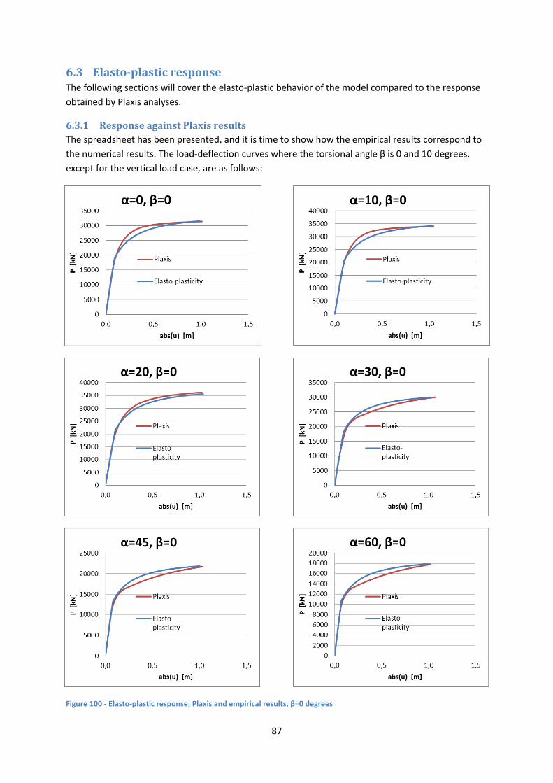
87
6.3 Elasto-plastic response The following sections will cover the elasto-plastic behavior of the model compared to the response
obtained by Plaxis analyses.
6.3.1 Response against Plaxis results
The spreadsheet has been presented, and it is time to show how the empirical results correspond to
the numerical results. The load-deflection curves where the torsional angle β is 0 and 10 degrees,
except for the vertical load case, are as follows:
Figure 100 - Elasto-plastic response; Plaxis and empirical results, β=0 degrees

88
Figure 100 shows the elasto-plastic behavior from Plaxis curves and empirical curves when the
torsional angle is 0 degrees. It is observed that the best curve fitting is obtained when the inclination
angle is between 20 and 30 degrees.
Figure 101 - Elasto-plastic response; Plaxis and empirical results, β=10 degrees
Figure 101 shows the elasto-plastic behavior from Plaxis curves and empirical curves when the
torsional angle is 10 degrees. The curve fitting for all the horizontal load cases interpolates the Plaxis

89
results in a proper way; the tendency is thus for the quality of the curve fitting to increase with the
torsional angle β.
6.3.2 Two-way loading
It can be concluded that the elasto-plasticity behaves accurately for proportional loading, especially
since the plastic anisotropy of the anchor response is disregarded, and instead optimized as a whole.
Since isotropic hardening is assumed, the formulation would, however, not provide realistic results
for two-way loading due to the Bauschinger effect. A load cycle in the x-direction is applied to
illustrate its limitation.
Figure 102 - Load cycle in the x-direction; Plaxis and empirical isotropic response
If cyclic two-way loads were expected, kinematic hardening would clearly be favorable due to the soil
parameters applied in this thesis.
6.3.3 Normality
Another interesting aspect of the Plaxis results is whether the normality assumption is applicable at a
macro level between padeye loads and padeye displacements. The soil parameters in the thesis
impose associate flow at element level since the dilatational angle equaled zero. The question is then
whether the normality assumption remains valid after all the elements have been integrated at the
global level. Some degree of discretization error will in any case be present, due to the finite element
discretization. The yield surface, which the Plaxis results will be compared against, will also contain a
degree of error; even though the chosen yield surface provides accurate results, the points are still
not interpolated exactly. Plastic displacement vectors in the xz-plane were normalized and plotted
against the yield surface when the rotational angle β was zero. The normalized plastic incremental
displacements were isolated by subtracting the incremental elastic displacements, obtained from the
stiffness matrix, from the total incremental displacements, and then normalized:
{ }
{ } [ ] { }
√ { } [ ] { } { } [ ]
{ }
(6.42)

90
The following normality is observed:
Figure 103 - Normality; plastic displacement vectors
Figure 103 shows that the normality assumption is valid for the global system. The elasto-plastic
formulation also assumes associated flow, which means that the plastic displacement increments will
be normal to the yield surface.
6.4 Elasto-plasticity: Summary The elasto-plasticity has been implemented in an Excel spreadsheet. The hardening rule is
represented by the hyperbola, and isotropic hardening is assumed. The second yield surface was
taken as the yield criterion, with the mobilization factor taken as the state parameter. The results for
proportional loading corresponded well, but were not appropriate in relation to two-way loading.
The normality assumption was applicable at the global level with respect to padeye loads and padeye
deflections.
-0,5
0,0
0,5
1,0
1,5
2,0
2,5
3,0
0,0 1,0 2,0 3,0 4,0 5,0
dV
an
d d
uz,
pla
stic
[m
]
dH and dux ,plastic [m]
Normality, β=0deg
F(Q)/10000
plaxis,alpha=0
plaxis,alpha=90
plaxis,alpha=10
plaxis,alpha=20
plaxis,alpha=30
plaxis,alpha=45

91
7 Generalization In this chapter, the results will be presented in a generalized way. The capacity will first be presented
in a non-dimensional way, before showing normalized capacity curves. Thereafter, the focus will be
on stiffness. Generalization of elasto-plasticity will then be dealt with. Finally, it will be shown how
the generalized response corresponds to suction anchors with aspect ratios L/D equal to three and
eight. Note that the generalization is still limited to undrained conditions.
7.1 Non-dimensional results Non-dimensional results will be presented in the following, thus making the results applicable to
situations with other anchor geometries and other soil conditions. It is debatable which parameters
the anchor should be generalized with respect to. For horizontal loads, it has been chosen to
generalize the results with respect to the width and the length of the anchor, as well as the average
shear strength. The generalization should provide a good fit for other anchors as well, since the flow-
around mechanism gives the same unit resistance with depth, while for shallow suction anchors, the
base shear will compensate somewhat for the decrease in earth pressure resistance. For vertical
loading, both the base resistance and the shaft resistance contribute significantly to overall capacity.
While the shaft resistance is dependent on both the length and the width of the anchor, the base
resistance is not directly dependent on the length, but is dependent on the width to the power of
two. The shaft resistance will also be dependent on the roughness of the wall, and might change
from project to project. The vertical results will be generalized on the basis of the same parameters
as for horizontal loading, and a simple diagram will be presented illustrating how the results may be
applicable to other suction anchors. Non-dimensional capacity coefficients are introduced:
(7.1)
(7.2)
For interaction between horizontal and vertical loads, the non-dimensional coefficient will be
obtained by combining equation 4.10 and 4.14.
√
√
(7.3)
where P is the magnitude of the failure capacity
N is a non-dimensional factor
L is the length of the anchor
D is the diameter of the anchor
is the average undrained strength.
The capacity curves from Plaxis can now be presented in a non-dimensional fashion:

92
Figure 104 - Non-dimensional HV space
Figure 105 - Non-dimensional capacity
The figures show the capacities in a non-dimensional way, and include the reduction in capacity due
to the other force components present. The non-dimensional capacity curves can now be used to
calculate capacity for other suction anchors. It should be noted that non-dimensional results will
overestimate capacity, due to the discretization error with finite elements. Comparisons against hand
calculations show that the vertical and the horizontal loads are overestimated by approximately 10%,
while the torsional moment is overestimated by 50%. If the capacity curves are used, these should be
adjusted for the discretization error.
The following expression makes the results from the vertical and the inclined loading applicable to
other projects:
(7.4)
0
1
2
3
4
5
6
0 2 4 6 8 10 12
V/(
L*D
*su
) [
kN/k
N]
H/(L*D*su) [kN/kN]
Non-dimensional HV space
beta=0
beta=5
beta=10
beta=20
beta=45
beta=90
0
2
4
6
8
10
12
14
0 15 30 45 60 75 90
P/(
L*D
*su
) [
kN/k
N]
alpha [deg]
Non-dimensional capacity P/(L*D*su)
beta=0
beta=5
beta=10
beta=20
beta=45
beta=90

93
It involves three terms; a shaft term, a base term and a weight term. A diagram with the following
assumptions is presented below: It is assumed that the weight ratio remains constant, that the ratio
between the shear strength at the base and the average shear strength is the same as for this
project, i.e. 32kPa/17kPa=1.89, and that the reversed end bearing coefficient is taken to be 9. The
following diagram is then obtained, with a roughness factor of the wall equal to r=0.4, 0.6 and 0.8,
respectively:
Figure 106 - Vertical capacity factor; wall roughness = 0.4, 0.6, 0.8, Nc=9, W'/(LDsu)=0.54, su(L)/su=1.89
Figure 106 shows that the vertical capacity factor changes significantly depending on the aspect
ratio.
7.2 Normalized strength The Plaxis results in the HV space can be normalized with respect to the maximum horizontal and
vertical force components. The maximum horizontal load that can be applied to the system is
38,000kN, while the maximum vertical force is 15,500 kN.
Figure 107 - Normalized results
2
3
4
5
6
7
8
9
10
2 3 4 5 6
Nv
[kN
/kN
]
L/D [m/m]
Vertical capacity factor
r=0.4
r=0.6
r=0.8
0,0
0,2
0,4
0,6
0,8
1,0
0,0 0,2 0,4 0,6 0,8 1,0
V/V
u [
kN/k
N]
H/Hu [kN/kN]
Normalized results
beta=0
beta=5
beta=10
beta=20
beta=45
beta=90

94
Figure 107 shows that horizontal loading at the padeye will mobilize the horizontal capacity at about
83%. This means that the vertical distance between the load attachment point and the neutral plane
reduces the moment by approximately 17%. The diagram does not capture the normalization due to
torsion. A change in the aspect ratio will change of torsional resistance differently than the
horizontal. The normalization is thus limited to suction anchors with an aspect ratio equal to 5 for the
load cases where the torsional angle is different from zero.
The empirical yield surface will, however, be capable of normalizing all the force components in a
proper way. The empirical yield surface interpolated the Plaxis results almost perfectly, and will be a
powerful tool in estimating the capacity of suction anchors with an arbitrary geometry and, at least,
for normally consolidated clay conditions. The following equation is presented:
(7.5)
where a, b c, and d are empirical coefficients, which gave values of 5, 5, 2 and 2,
respectively, due to curve fitting
hx, hy, v, t, my and mx are normalized force components, resulting from the
following expressions:
(7.6)
| |
The ultimate force components and the eccentricities for a given project can then be inserted into
the equations, thus obtaining the capacity surface. The surface can also be presented in the HVT-
space:
(7.7)
where √
and √
The latter equation imposes an insignificant adjustment of the original yield surface, since the
resultant direction of the moment and the direction of the horizontal force will, in general, not
coincide. However, this can safely be disregarded. The normalized HV space with constant torque-
mobilization curves will now be shown:

95
Figure 108 - Normalized HV space with constant mobilized torque
The ultimate force components can be roughly estimated from the following equations:
(7.8)
(7.9)
(7.10)
(7.11)
(7.12)
where Hu, Vu, Mu and Tu are ultimate force components
is the horizontal capacity factor, which can be given a value in the range of 10-11,
although this study has given it a value of 38,000/(30*6*17)=12.4
z* is the distance between the seabed and the load attachment point
is, in this context, the distance from the seabed to the plastic neutral plane minus
the distance from the seabed to the padeye
is the horizontal distance between the neutral axis and the load attachment point
α is the roughness factor for the shafts
W’ is the effective weight of the anchor
Nc is the reverse end bearing capacity factor, often taken to be 9
Tpadeye is the torsional resistance due to the area of the padeye, which may be
disregarded
Note that the equation for the bending moment was derived for a linearly increasing earth pressure
resistance per unit length. For situations were the earth pressure per unit length can be considered
as constant, the ultimate capacity would be 0.25LHu, obtained from limit equilibrium. How the
normalized yield surface can be applied in practice, will be showed by varying the padeye location
based on the properties addressed by the thesis:
0
0,2
0,4
0,6
0,8
1
1,2
0 0,2 0,4 0,6 0,8 1
v [
kN/k
N]
h [kN/kN]
Normalized HV space with torque
t=0
t=0.2
t=0.4
t=0.6
t=0.8
t=0.99

96
Figure 109 - Parametric padeye positions, ez=0-5 meters
A quite interesting conclusion can be drawn from the figure; that it would be beneficial to lower the
padeye position in response to any kind of inclined loading. The vertical plastic eccentricity for this
project is 3 meters from the plastic neutral plane. The optimum padeye position for most kinds of
inclined loading will be one meter above the neutral plane. Due to horizontal loads, the optimum
padeye position will be at the neutral plane; which is the definition of the plastic neutral plane. A
padeye position 2 meters below the plastic neutral plane was included as well; the curve shows that
an increase in the vertical load causes a larger bending moment, rather than unloading of the
bending moment as observed when the padeye position is above the neutral plane. This can also be
shown by the constraint loading equations.
It is also interesting to use the empirical yield surface with respect to the hand calculations obtained
in this thesis. The ultimate components are inserted in equation 7.6, and compared against the Plaxis
results:
Figure 110 - Plaxis results compared to hand calculations
0
2000
4000
6000
8000
10000
12000
14000
16000
18000
0 10000 20000 30000 40000
V [
kN]
H [kN]
Parametric padeye position
ez=0m
ez=1m
ez=2m
ez=3m
ez=4m
ez=5m
ez=-2m
0
2000
4000
6000
8000
10000
12000
14000
16000
18000
0 10000 20000 30000 40000
V [
kN]
H [kN]
Plaxis results vs hand calculations beta=0,plaxis
beta=5,plaxis
beta=10,plaxis
beta=20,plaxis
beta=45,plaxis
beta=90,plaxis
beta=0
beta=5
beta=10
beta=20
beta=45
beta=90

97
Figure 110 show that the capacity curves overestimates is entire load space compared to the hand
calculations, and that the system is more sensitive in terms of misorientation with respect to the
installation.
7.3 Non-dimensional stiffness It can also be useful to present the stiffness of the system in a non-dimensional manner. It will then
be possible to measure the displacements for small loads, and the elasto-plastic stiffness matrix will
be given for arbitrary suction anchors (formulas will not be numbered).
Several factors have an influence on the stiffness of the system:
Soil conditions
Stiffness profile
Type of loading
Geometry of the anchor
The non-dimensional stiffness of the system will be limited to the undrained condition, which implies
that the applied loads can be considered short-term loads. When the loads are acting on the system
for a sufficiently long period of time, the soil will start to consolidate, and the displacements will be
extended without any change in external loading. The stiffness profile of the soil and the geometry of
the anchor will obviously have an impact on stiffness. The stiffness profile for this project is as
follows:
[ ] (7.13) (7.14)
where G is the shear modulus
K is the bulk modulus, which can be regarded as infinite, due to the undrained
conditions
n is a constant, which implies that G is proportional to the strength
The average shear stiffness will be used in defining the non-dimensional stiffness of the system. The
most significant anchor geometries for this project are the length and the diameter of the anchor. It
has already been shown that the suction anchor can be considered as rigid, which means that the
stiffness of the anchor is much greater than the stiffness of the surrounding soil. The stiffness
equation for the system is as follows:
{ } [ ]{ } (7.15)
where { } is the load vector at the padeye
[ ] is the stiffness matrix
{ } is the displacement vector at the padeye
It might be convenient for formulation purposes if all terms in the stiffness equation are non-
dimensional. This will be accomplished if both the load vector and the displacement vector are non-
dimensional. The following generalization can be chosen:
{ } { }
{ }
{ }
(7.16)

98
where { } is the non-dimensional load vector determined by the length, the diameter and
the average shear stiffness
{ } is the non-dimensional displacement vector determined by the diameter
The non-dimensional system equation will then be:
{ } [ ]{ } [ ] [ ]
(7.17)
The following non-dimensional stiffness matrix is obtained by insertion:
[ ] [
] (7.18)
The stiffness matrix for a project can then be expressed as follows:
[ ] [
] (7.19)
Since the shear modulus and the shear strength profile are proportional, the stiffness matrix can also
be specified in terms of the proportional factor, the length and the average shear strength:
[ ] [
] (7.20)
where n is the proportional factor between the shear modulus and the shear strength,
which equals 100 for this project
The model applied for the thesis focuses on the ultimate state. A larger soil volume should be applied
if the focus is on the stiffness properties. The obtained matrix is for that reason likely to overestimate
the stiffness, and should not be used for other projects without adjustment.
The obtained matrix is defined in terms of padeye loads and deflections. The matrix is only suited for
other projects if the eccentricities between neutral planes and load attachment points are the same,
relative to the anchor geometries. This is highly unlikely, and a stiffness relation in terms of loads and
responses at the optimum load attachment point would for that reason be more suited. The
optimum load attachment point in this sense is where the three neutral planes intersect. The
stiffness matrix at this point can then be transposed to any point at the suction anchor, under the
assumption that the anchor can be considered rigid.
The displacements are therefore constrained. The constraint relations between the padeye and the
optimum load attachment point will be shown. Both the loads and the displacements will be
constrained. The displacement relations are as follows:

99
{
}
{
}
(7.21)
The expression can also be stated the other way around:
{
}
{
}
{
}
(7.22)
There is a similar relation between forces applied at the padeye and force resultants:
{
}
{
}
(7.23)
The equation states that an applied force vector at the padeye can be expressed as a transformed
force vector at the optimum load attachment point.
One assumption is required to determine the stiffness matrix; namely an uncoupled stiffness matrix
at the optimum load attachment point. Due to the padeye plate, the system is not fully symmetrical,
but this will not influence the coupling significantly. The neutral plane normal to the z-axis is defined
as the plane that causes translations without rotations due to horizontal loads. The uncoupling
assumption is thus appropriate. Plaxis results confirm the assumption.
{
}
[
]
{
}
(7.24)
{
}
[
]
{
}
(7.25)
where Kh is the horizontal stiffness
Hv is the vertical stiffness
Km is the bending stiffness
Kt is the torsional stiffness
The stiffness coefficients are determined from load-deflection curves.

100
Inserting the constraint equations, the following system equations are obtained between the padeye
load and the deflection:
{
}
[
]
{
}
(7.26)
And finally:
[
]
(7.27)
where , , and are the elastic stiffness coefficients resulting from the force
components of the anchor
is the eccentricity in the x-direction between the padeye and the neutral plane;
3.75 m
is the eccentricity in the z-direction between the padeye and the elastic neutral
plane, which is defined as the plane that causes translation without rotation due to
horizontal loads.
The padeye position is not restricted to a fixed position under this formulation, which makes the
formulation general with respect to anchor geometry and the stiffness profile of the soil.
Note that the definition of ez in terms of capacity was different from the elastic definition. In the
latter case, ez was the eccentricity between the load attachment point and the plastic neutral plane,
which is the plane that provides the largest horizontal capacity.
Figure 111 - The suction anchor; difference between elastic and plastic eccentricities

101
The planes will, in general, not coincide. This can be illustrated by comparing the responses caused
by an applied bending moment, where the soil is first modeled as linearly elastic, then as elasto-
plastic, with the moment giving rise to a failure mechanism. The plastic eccentricity, which was
presented in section 4.3, is 3.0 meters, while the elastic eccentricity is 2.2 meters.
Figure 112 - Response caused by applied bending moment; (a) failure mechanism, (b) linearly-elastic response
7.4 Elasto-plasticity generalization The generalization presented so far can also be implemented in the elasto-plastic formulation. A
generalized stiffness matrix, yield surface and normalized ultimate strength have been presented,
and only the hardening remains to be determined. The hardening rule in the elasto-plastic
formulation was obtained by curve fitting between the mobilization factor and the displacements. If
the displacements are normalized, for instance with respect to the diameter of the anchor, the
hardening rule is also obtained. Other considerations, like for instance whether kinematic hardening
should be applied, will be the same for the conventional formulation.
The spreadsheet made for the project was implemented in a generalized way; the empirical
coefficient, the ultimate components, the stiffness matrix and the eccentricities can all be easily
changed for purposes of another project. However, the hardening rule needs to be determined.

102
8 Discussion In this chapter, the results from the project will be evaluated. Firstly, the modeling considerations
will be discussed. The reliability of the model and the results will be addressed, before the tendencies
of the results will be presented. These include tendencies of the load-deflection curves, the failure
mechanisms and the capacity curves. The empirical data will then be addressed, before discussing
generalization.
8.1 Modeling considerations Modeling considerations are examined prior to analyses. Simplifications will always be necessary,
however it is important that the physical behavior remains modeled in a proper way, and that
operation of the model is not too time-consuming. This section discusses some of these
considerations.
Geometrical nonlinearities due to combined loading have been disregarded. The geometrical
nonlinearities will have a large impact on some of the load cases; when a vertical pull-out load is
applied, the contact area between the shaft and the soil will decrease, implying that a lower capacity
will be obtained when implementing the nonlinearity, due to displacement boundaries. The
geometrical load boundaries will also be important for the load cases where a large torsional
moment is present. The failure mechanism of the anchor is then governed by anchor rotation about
the z-axis. During rotation, the misorientation of the anchor will decrease, implying that the torque
will also decrease. This response will only be obtained if geometrical nonlinearities are included.
Geometrical nonlinearities will only be important for large deformations, and will be more time-
consuming to model. The load cases where the load vectors were pointed in the y- and z-directions
were additional to conventional analyses, calculated with the updated mesh option. The updated
mesh option will update the mesh due to the deformed geometry, and the strain measure is also
different; nonlinearities between displacements and strains will be accounted for. The following
response was obtained:
Figure 113- Updated and unchanged mesh for vertical load case
0
2000
4000
6000
8000
10000
12000
14000
16000
18000
20000
0,0 0,5 1,0 1,5 2,0 2,5
V [
kN]
padeye displacement [m]
Updated and unchanged mesh
updated mesh, vertical
unchanged mesh, vertical

103
Figure 113 shows that the updated mesh gives a reduced capacity for the vertical load case. The
difference between the curves is especially prominent when the padeye has deflected about one
meter. The updated mesh calculation had approximately reached the failure state when deflected
one meter and a further increase in load would result in infinite deflections; the system is singular.
The ultimate capacity with the updated mesh is 14,700 kN, which means that the conventional
calculation, with failure taken as one meter padeye deflection, overestimated the capacity by about
5%. It might thus be appropriate to adjust the failure definition for purposes of later projects. For
instance, failure can be defined as D/10. It should be noted that the simple material model; the
linearly-elastic Mohr-Coulomb model, does not account for softening at large shear strains. This
means that in reality, the true load-deflection curve would most likely have an even larger softening
response. The load case where loading was pointed in the y-direction gave the following response
under the updated mesh option, compared to the conventional calculation:
Figure 114 - Updated and unchanged mesh for the load case pointed in y-direction
Figure 114 shows that the geometrical nonlinearities are of benefit to the system for large torsional
angles. After a horizontal yielding plateau, the system shows a hardening behavior due to a decrease
in the eccentricity between the loading line and the neutral axis.
The response changes significantly for large deflections. However, since failure was defined as one
meter padeye deflection, the analysis without geometrical nonlinearities will have a limited impact. A
smaller deformation criterion might be adopted in order to limit the differences between the
analyses. Alternatively, a correction factor, which accounts for the nonlinearity, can be introduced.
Soil volume of the model is also a major consideration. In order to achieve the best failure
mechanisms, it is important that the element mesh is dense where the failure mechanisms are
expected. However, it would also be important, due to stiffness, to have a sufficiently large soil
volume, in order to capture deflections that will have an influence on the response. The main focus
of the thesis was on capacity. Soil volume of the model was therefore chosen for reasons of capacity,
and the stiffness obtained should either be adjusted to reflect the distances to the boundaries, or
calculated by other methods.
0
1000
2000
3000
4000
5000
6000
7000
0,0 0,1 0,2 0,3 0,4 0,5
Hy
[kN
]
padeye displacement [m]
Updated and unchanged mesh
updated mesh, Hy
unchanged mesh, Hy

104
The geometry of the anchor was modeled with few simplifications. The ring stiffeners used for
installation stability purposes were omitted, since the installation phase in Plaxis does not simulate
the self-weight and the suction penetration. Compression forces in the anchor due to installation will
therefore not be present. This simplification makes the modeling of the anchor more convenient.
37 load combinations were chosen for the main analyses. The load cases were designed to map the
entire load space with regard to tensile forces. Even though large torsional angles due to
misorientation are highly unlikely, these were still included in order to obtain the response in the
entire load space. The load cases were constructed in such a way as to have the most load cases
where needed. For instance, since the failure mechanism and the vertical capacity were more or less
exactly the same whether the inclination angle was 60 or 90 degrees, there was no need for load
cases in between these. The same can be said for the torsional angle; most of the capacity due to
torsional resistance was mobilized when the torsional angle was 20 degrees, and only one torsional
angle was placed in between, in order to obtain a smoother capacity surface.
8.2 Reliability of the model In any numerical study, it is essential to evaluate the reliability of the results. The reliability of the
results can first be compared against hand calculations. Mesh refinements are also essential for the
finite element model. It will also be important to examine the responses, and look for unphysical
behavior. This can for instance be irregularities in the load-deflection curves, unreasonable changes
in stress states caused by loads, unrealistic failure mechanisms, interface mobilization, continuity of
the anchor, etc. If any one of the said responses gives answers that cannot be explained, something
is likely to be wrong with the model.
The results from the hand calculations gave answers that differed slightly from the corresponding
load cases in Plaxis with the model of 20,500 soil elements:
Force component Hand
calculation Plaxis Error [%]
Horizontal [kN] 34,000 38,000 12
Vertical [kN] 14,000 15,400 10
Bending moment [kNm] 204,000 230,000 12
Torque [kNm] 16,000 23,800 49 Figure 115 - Results from hand calculations and from Plaxis
Figure 115 compares the hand calculated results to the results from Plaxis. The results from Plaxis are
10-12% overestimated compared to the corresponding hand calculation, except for the torsional
moment, which is overestimated by 49%. It should be noted that the hand calculations are not exact
solutions either, and that 10-12% does not mean that the discretization error of the model is 10-12%.
Nonetheless, the discretization error of the torsional resistance is more than one would desire. As
described in the theoretical chapter, the resistance caused by torsion is due to three features; the
shaft resistance, the base resistance, and the resistance due to the padeye. The shaft resistance
contributed most significantly. It was suspected that the large error was caused by the padeye, and a
load case with torsion, where the padeye plate was not activated was executed.

105
Figure 116 – Respnce with and without the padeye with respect to torsion, inc disp; (a) with padeye (b) without padeye, (c) response
Figure 116 shows that the torsional stiffness will be calculated accurately if the padeye is not
activated. At failure, a flow around mechanism is developed around the padeye. It turns out that a
very fine mesh is needed around the plate in order to compute the response accurately. It would for
that reason be better to not model the padeye at all. Equivalent padeye loads could rather be applied
as a set of load vectors.
The mesh refinements could indicate that the model offered a good convergence. However, a slow
convergence rate might also be a possibility, which could convey a false impression. five mesh
refinements were executed and compared in section 4.7. It was observed that the horizontal load
0
5000
10000
15000
20000
25000
30000
0,0 2,0 4,0 6,0
T [
kNm
]
padeye delfection [m]
The effect of padeye due to torsion
without padeye
with padeye

106
case for mesh refinement number three actually gave a more accurate answer than mesh refinement
number four. Due to the nature of finite elements, the response should move towards correct results
when the number of elements increases in a uniform way. However, the users of Plaxis 3D have
limited control over the meshing options, and the difference between the mesh refinements will not
be increased in a uniform way. Uniform mesh refinements are not desired either, since it is more
important to increase the density of the mesh where the critical response is located. In the case of
mesh refinement number four, the elements where positioned in a way that favored the vertical
failure mechanism more than the horizontal one. Since mesh refinement number four was
substantially more time consuming and provided only slightly better accuracy, mesh refinement
number three was chosen for the main analyses. Mesh number five was too time-consuming for this
parametric study.
8.3 Observations of the capacities The capacity curves were given in terms of a load vector applied at the padeye position, with the
inclination angle and the torsional angle mapping the entire load space for tensile forces. First of all,
it was shown that the horizontal load-deflection curves for horizontal loading had a better defined
yield plateau than for vertical loading. This can be explained by the failure mechanisms; the
horizontal failure mechanism, consisting of the wedge mechanism at the upper part, and the flow-
around mechanism at the lower part, is closer to a rigid slip-plane mechanism than the vertical
failure mechanism, which mechanism involves soil movements into the anchor, thus implying that
the capacity will constantly increase with larger deflections. However, when the geometrical
nonlinearities are included, the softening response will dominate after approximately one meter of
padeye deflection.
The failure mechanisms can roughly be divided into four categories:
Vertical failure mechanism, where the soil plug translates with the anchor, and a classical
reversed end-bearing capacity is observed.
Horizontal failure without anchor rotation, involving a wedge mechanism that gradually
converts into the flow-around mechanism.
Horizontal translations with rotations. The rotation center is then close to the anchor. The
horizontal capacity is then reduced in order to maintain equilibrium due to the moment.
Torsional failure mechanism, where the anchor rotates about the z-axis.
Vertical failure dominates when the load inclination angle is 30 degrees or more, and the maximum
horizontal force is observed when the inclination angle is 20 degrees, due to the unloading of the
bending moment, which is more beneficial than vertical loading with respect to capacity. When the
inclination angle is zero, the rotation center is almost at the anchor base, and the soil at the lower
part is not mobilized in any significant way. A torsional angle of 5 degrees does not reduce the
capacity to any large extent; when the inclination angle is zero, the capacity is reduced by 4%. When
the torsional angle is 10 degrees, the maximum reduction is present when the inclination angle is 20
degrees; the capacity has now been reduced by 16%, which is a relatively large reduction. When the
torsional angle is further increased to 20 degrees, only half of the capacity is left for the horizontal
load cases, and the capacity and the corresponding failure mechanism are totally governed by the
torsion. It should be noted that torsional angles of these magnitudes are definitely not realistic in
practice, and are primarily included to obtain a complete surface, and to gain a deeper

107
understanding of the system. The torsional resistance of the system is likely to overestimate capacity
more than the other force components, when considering comparisons against hand calculations.
This implies that the true torque reduction will be increased. However, the normalized curves are still
applicable, where the ultimate forces are either hand calculated or obtained by numerical studies.
The normalized curves will then interact with all six force components in a constrained way, since the
loads will be applied at the padeye.
8.4 Evaluation of the empirical data Two different yield surfaces were considered, both focusing of the relation between the six different
force components of the system. Constrained loading conditions were then introduced, and both
yield surfaces could be expressed in terms of three unknowns. The three translational forces were
chosen, since these are the forces imposed as a load vector at the padeye. When the three padeye
forces are represented in space, information will actually be provided on all the six force
components. The first yield surface had a simpler form than the second one, but the second provided
by far the most accurate curve fitting. Comparisons between them can be made, assuming
mobilization f=1:
Yield Surface 1 Yield Surface 2
( ( )
)
( ( )
)
Simple form Slightly more extensive
Easy to implement in elasto-plasticity Time consuming to implement
Provides a decent curve fitting Provides excellent curve fitting
No physical foundation Has a physical foundation
Figure 117 - Comparisons yield surfaces
Both capacity curves are quite good, although the second yield surface is more accurate. Optimizing
showed that the average expected error for a load case was only 0.7%.
The elastic stiffness coefficients were obtained by examination of load cases in the three normal
directions, where linear curves were curve fitted based on the initial response of the load-deflection
curves. The flexibility and stiffness matrix were then obtained. It was chosen to measure the loads
and the displacement directly from the padeye. It would also be possible to load and measure the
response at the optimum load attachment point, and then transpose the response to the padeye.
The latter method would be generally applicable to other projects, although the eccentricity ez
would also be needed.
The curve fitting between the mobilization factor and the plastic deflections was based on elasto-
plasticity. Power law, Voce rule and hyperbola were all considered. The hyperbola offered the most

108
suitable shape and gave the best estimation through the method of least squares. The same
hardening rule with the same coefficients was applied in all directions.
Elasto-plasticity in terms of padeye loads and deflections was implemented by isotropic hardening,
although specific load cycles in Plaxis indicated that kinematic hardening would be more appropriate.
However, since the anchor will be loaded from a mooring chain, two-way loads are not likely due to
loads from the platform.
8.5 How to apply the generalized results Generalized results were presented in chapter 7. The generalized results can be applied in other
projects, and a lot of time can be saved. However, it is important to first understand that the non-
dimensional results obtained from this study are upper bound solutions. Adjustments and
comparisons are thus required. The second curve-fitted capacity curve will, however, be a powerful
tool, which can be used to estimate the capacity surface. The fact that the generalization directly
reflects the padeye loads makes it especially practical to use.
The values of the stiffness coefficients are likely to be overestimated, because of the distances to the
boundaries, which is just in excess of six diameters. In other words, the model is sufficiently large for
capacity, but will overestimate stiffness.
The generalized stiffness matrix, in which the eccentricities can easily be changed from project to
project, may also be useful; if the various stiffness coefficients are known, the stiffness matrix with
regard to any padeye position can be obtained. However, the elastic neutral plane is then needed.
109
9 Conclusion & further work
9.1 Conclusion Capacity curves in Plaxis 3D for a suction anchor with an aspect ratio equal to 5 have been obtained,
based on ultimate loads applied at the padeye, which is located approximately 2/3 of the anchor
length from the seabed. The thesis is limited to undrained loading conditions. A parametric variation
of the load directions has been executed, so that the entire loading space defined by tensile forces
has been studied. The capacity curves show that misorientation of the anchor caused by the mooring
plane will reduce capacity by about 3% when such misorientation is 5 degrees and 12% when such
misorientation is 10 degrees, due to horizontal and slightly inclined loads. There is in practice no
reduction in capacity when the inclination angle is 45 degrees or more, for realistic torsional angles.
Two empirical curves have been determined in order to make the results applicable to other
projects. The empirical formulas combine the six force components present in terms of padeye loads.
Due to eccentricities to the three neural planes, there will be three forces and three moments
present. One of the empirical curves interpolated all the Plaxis results with an average error of 0.7%,
consisting of four empirical coefficients. This yield surface has been used to derive an elasto-plastic
formulation, in terms of padeye loads and padeye deflections. Isotropic displacement hardening has
been applied, and a general Excel spreadsheet has been established. The elastic and the plastic
relationships have been determined from curve fitting.
The results have been further generalized, so that the work in the thesis can be used for other
suction anchors. The normalized capacity curve, in particular, can be efficiently used in other
projects.
The reliability of the results is mainly acceptable, although the torsional moment is overestimated by
about 50%, due to the discretization error. It is showed that the overestimation is mainly due to the
flow around mechanism of the padeye.
9.2 Further work In further work, the numerical modeling can be executed in other programs, a kinematic hardening
formulation can be constructed and experiments based on combined loading can be performed.
More advanced material models can be applied, and capacity curves can be designed for drained
conditions as well.

110
References Andersen, K.H. & Jostad H.P. (2002). Shear Strength Along Outside Wall of Suction Anchors in Clay
after Installation. Proceedings of the Twelfth (2002) ISOPE Conference.
Andersen, K.H. & Jostad H.P. (2004). Shear Strength Along Inside of Suction Anchor Skirt Wall in Clay. Offshore Technology Conference, Paper OTC 16844 Andersen K.H., Murff, J.D., Aubeny,C., Randolph, M.F., Supachawarote, C., Sharma, P., Jostad H.P.,
Clukey E.C., Erbrich, C. T. & Hansen, B. (2005). Suction anchors for deepwater applications. Proceedings of the International Symposium. on Frontiers in Offshore Geotechnics (IS-FOG 2005), 3-30
Aubeny, C & Murff, D. (2005). Suction Caissons & Vertically Loaded Anchors: Design Analysis
Methods, Department of Civil Engineering Texas A&M University Augustin, L.C. (1828). Exercises de mathématiques. Paris: Bure frères
Cook, R.D., Malkus, D.S., Plesha, M.E. & Witt, R.J. (2001). Concepts and Applications of Finite Element Analysys (4nd edition). New York: John Wiley & Sons
Coulomb, C.A. (1776). ssai sur une application des r gles de maximis & minimis uel ues
probl mes de stati ue, relatifs l architecture. Paris: De l'Imprimerie Royale
Dean E.T.R. (2009). Offshore Geotechnical Engineering. London: Thomas Telfond Deng, W. & Carter J. P. (2000). A Theoretical Study of the Vertical Uplift Capacity of Suction Caissons.
Proceedings of the 10th International Offshore and Polar Engineering conference, 342-349 El-Sherbiny, R.M., Vanka, S.K., Olson, R.E. & Gilbert, R.B. (2005) Capacity of suction caissons under
inclined loading in normally consolidated clay. Proceedings of the International Symposium. on Frontiers in Offshore Geotechnics (IS-FOG 2005), 281-287
Irgens, F. (2008). Continuum Mechanics. Berlin: Springer
Leffler, Pattarozzi, W.L., Sterling R. & Gordon. (2011). Deepwater Petroleum Exploration and
Production (2nd Edition). Tulsa: PennWell.
Jeanjean, P. (2006). Setup Characteristics of Suction Anchors for Soft Gulf of Mexico Clays: Experience from Field Installation and Retrieval. Offshore Technology Conference, Paper OTC
18005
Jostad H.P & Andersen, K.H. (2002). Foundation Design of Skirted Foundations and Anchors in Clay. Offshore Technology Conference, Paper OTC10824
Kreyszig, E. (2006). Advanced Engineering Mathematics (9nd edition). Singapore: John Wiley & Sons
Lee, Y.C., Tjok, K.M. & . Audibert J.M.E (2005). Lessons learned from several suction caisson installation projects in clay. Proceedings of the International Symposium. on Frontiers in Offshore Geotechnics (IS-FOG 2005), 235-239

111
Martin, C. M. & Randolph, M. F. (2006). Upper-bound analysis of lateral pile capacity in cohesive soil. Geotechnique, 56(2), 141–145
Nordal, S. (2010). Lecture Notes PhD course BA8304 Soil Modeling. Trondheim: Norwegian University
of Science and Technology, Geotechnical Division Plaxis. (2010). Plaxis reference manual. Plaxis. (Unknown). About Plaxis - History. Obtained 25th April 2013, http://www.plaxis.nl/page/4863/ Poisson, D.S (1833). Traite de mecanique (2nd edition). Paris: Bachelier, Imprimeur-Libraire
Poulos, H.G., & Davis, E.H. (1974). Elastic Solutions for Soil and Rock Mechanics. New York: John
Wiley
Randolph, M.F.,.O'Neill M.P., Stewart D.P. & C.Erbrich. (1998). Performance of Suction Anchors in Fine-Grained Calcareous Soils. Offshore Technology Conference. , Paper OTC8831
Randolph, M.F. & Gourvenec, S. (2011). Offshore Geotechnical Engineering. New York: Spon Press
Rankine, W. (1857). On the stability of loose earth. Philosophical Transactions of the Royal Society of
London, 147, 9-27
Supachawarote, C., Randolph, M.F. & Gourvenec S. (2004). Inclined Pull-out Capacity of Suction Caissons. Proc. Int. Symp. Offshore Polar Eng., 2, 500-506
Taiebat, H.A. & Carter, J.P. (2005). A failure surface for caisson foundations in undrained soils.
Proceedings of the International Symposium. on Frontiers in Offshore Geotechnics (IS-FOG 2005), 289-295
Terzaghi, K. (1943). Theoretical Soil Mechanics. New York: John Wiley and Sons
Thorel, L., Rault, G., Garnier, J. & Bisson, A. (2005). Vertical uplift capacity of suction caisson in clay. Proceedings of the International Symposium. on Frontiers in Offshore Geotechnics (IS-FOG 2005), 273-279
Wilson, J.F. (2003). Dynamics of Offshore Structures (2nd edition). New Jersey: John Wiley & Sons
Wood, D.M. (2009). Soil Mechanics; A One-Dimensional Introduction. Cambridge: Cambridge
University Press
Young, T. (1845). A course of lectures on natural philosophy and the mechanical arts. London: Taylor
and Walton
Zdravkovic, L. & Potts, D.M. (2005). Parametric finite element analyses of suction anchors. Proceedings of the International Symposium. on Frontiers in Offshore Geotechnics (IS-FOG 2005), 297-302
Zienkiewicz, O.C., Taylor, R.L. & Zhu, J.Z. (2005). The Finite Element Method: Its Basis and
Fundamentals (6. edition). USA: Elsevier Zienkiewicz, O.C. & Taylor, R.L. (2005). The Finite Element Method for structural mechanics (6.
edition). USA: Elsevier

112
10 Attachments
Attachment A ……………………………………………………………………………………………………………… 113
Attachment B …………………………………………………………………………………………………………………114
Attachment C ………………………………………………………………………………………………………………….115
Attachment D ………………………………………………………………………………………………………………….116
Attachment E ………………………………………………………………………………………………………………….117

113
10.1 Attachment A - Horizontal capacity (Deng & Carter, 2000) Course increments, showed as an ilustration
z [m] Nps Su(z) q(z) [kN/m] v(z) M(z)
0 2,35 2 28,2 28,2 28,2
1 4,76 3 85,7 113,9 142,1
2 6,46 4 155,1 269,0 411,2
3 7,66 5 229,8 498,9 910,0
4 8,51 6 306,2 805,1 1715,1
5 9,10 7 382,2 1187,3 2902,4
6 9,52 8 456,9 1644,2 4546,6
7 9,81 9 530,0 2174,2 6720,8
8 10,02 10 601,4 2775,6 9496,4
9 10,17 11 671,2 3446,8 12943,2
10 10,27 12 739,7 4186,5 17129,7
11 10,35 13 807,0 4993,5 22123,2
12 10,40 14 873,4 5866,9 27990,1
13 10,43 15 939,0 6805,9 34796,0
14 10,46 16 1004,1 7810,0 42606,0
15 10,48 17 1068,7 8878,7 51484,7
16 10,49 18 1132,9 10011,6 61496,2
17 10,50 19 1196,9 11208,4 72704,6
18 10,50 20 1260,6 12469,0 85173,7
19 10,51 21 1324,2 -19647,8 109715,7
20 10,51 22 1387,7 -18260,2 91455,5
21 10,51 23 1451,0 -16809,1 74646,4
22 10,52 24 1514,3 -15294,8 59351,6
23 10,52 25 1577,6 -13717,2 45634,4
24 10,52 26 1640,8 -12076,4 33558,0
25 10,52 27 1704,0 -10372,3 23185,7
26 10,52 28 1767,2 -8605,1 14580,6
27 10,52 29 1830,4 -6774,8 7805,8
28 10,52 30 1893,5 -4881,2 2924,6
29 10,52 31 1956,7 -2924,6 0,0
30 10,52 32 2924,6 0,0 0,0
Vmax [kN]= 33441,0 -44189,9 Mst

114
10.2 Attachment B - Incremental displacements, horizontal planes Incremental displacements for horizontal planes, located at z=-5m, z=-10m and z=-15m
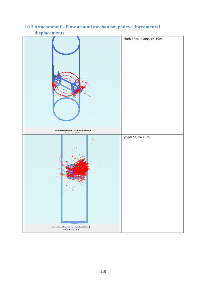
115
10.3 Attachment C - Flow around mechanism padeye, incremental
displacements
Horizontal plane, z=-19m.
yz-plane, x=3.5m.

116
10.4 Attachment D - Example elasto-plasticity Input:
Imput, ceofficients:
Input, load history Type Value
Load step dHx dHy dV
fo [] 0,6
1 15000 0 0
a [] 5,0
2 -35000 0 0
b [] 5,0
3 45000 0 0
c [] 2,0
4 -53000 0 0
d [] 2,0
5 58000 0 0
Hu [kN] 38000
6 -61000 0 0
Vu [kN] 15400
7 62500 0 0
Mu [kNm] 230000
8 0 0 0
Tu [kNm] 23800
9 0 0 0
ex [m] 3,75
10 0 0 0
ez [m] 3
tot 31500 0 0
k1 [] 2,056 k2 [] 0,393 Stiffness matrix: 211443 0 13744
K [kN/m]= 0 60000 0 13744 0 130893 Flexibility matrix:
4,76E-06 0 -5,00E-07 F [m/kN]= 0 1,67E-05 0 -5,00E-07 0 7,69E-06 Output:

117
10.5 Attachment E - Deflection space Plaxis, β=0
-40000
-30000
-20000
-10000
0
10000
20000
30000
40000
-0,20 -0,10 0,00 0,10 0,20 0,30Hx
[kN
]
ux [m]
Hx-ux
load step 1
load step 2
load step 3
load step 4
load step 5
load step 6
load step 7
load step 8
load step 9
load step 10
-0,1
0,0
0,1
0,2
0,3
-0,1 -0,1 0,0 0,1 0,1 0,2 0,2 0,3 0,3
uz
[m
]
ux [m]
deformations
alpha=0
alpha=10
alpha=20
alpha=30
alpha=45
alpha=60
alpha=90


